A projected Euler Method for Random Periodic Solutions of Semi-linear SDEs with non-globally Lipschitz coefficients 222This work was supported by Natural Science Foundation of China (12071488, 12371417, 11971488). YW would like to acknowledge the support of the Royal Society through the International Exchanges scheme IES\R3\233115.
E-mail addresses: y.j.guo@csu.edu.cn, x.j.wang7@csu.edu.cn, yue.wu@strath.ac.uk.

Yujia Guoa, Xiaojie Wanga, and Yue Wub
a School of Mathematics and Statistics, HNP-LAMA, Central South University, Changsha,
Hunan, P. R. China
b Department of Mathematics and Statistics, University of Strathclyde, Glasgow G1 1XH, UK
Abstract

The present work introduces and investigates an explicit time discretization scheme, called the projected Euler method, to numerically approximate random periodic solutions of semi-linear SDEs under non-globally Lipschitz conditions. The existence of the random periodic solution is demonstrated as the limit of the pull-back of the discretized SDE. Without relying on a priori high-order moment bounds of the numerical approximations, the mean square convergence rate is proved to be order $0.5$ for SDEs with multiplicative noise and order $1$ for SDEs with additive noise. Numerical examples are also provided to validate our theoretical findings.

Keywords: Projected Euler method, Random periodic solution, Stochastic differential equations, Pull-back, mean square convergence order.

AMS subject classification: 37H99, 60H10, 60H35, 65C30.

1 Introduction

Periodic occurrences abound throughout nature. Since the pioneering works of PoincarΓ© [14], periodicity has consistently remained a focal point in the examination of dynamical systems. It has garnered significant interest in various fields including thermodynamics [15], porous media [1], quantum time crystals [12], Thomas-Fermi plasma [16], and numerous other domains. Nonetheless, many real-world issues are prone to random fluctuations induced by uncertainty and unknown variables. Hence, the exploration of random periodicity emerges as a fundamentally crucial area of study.

As the stochastic counterpart to periodic solutions, the definition of random periodic solutions for a $C^{1}$-cocycle was initially proposed by Zhao and Feng [19], while Feng, Zhao, and Zhou [9] subsequently expanded upon this concept for semiflows. Their work has catalyzed further advancements in the exploration of various issues within autonomous and non-autonomous stochastic differential equations. This includes investigations into the existence of random solutions generated by non-autonomous SPDEs with additive noise [7], the anticipation of random solutions of SDEs with multiplicative linear noise [6], periodic measures and ergodicity [8], among others.

Given $W:\mathbb{R}\times\Omega\rightarrow\mathbb{R}^{d}$ a standard two-sided Wiener process on the probability space $(\Omega,\mathcal{F},\mathbb{P})$, where the filtration is defined as β„±st:=σ​{Wuβˆ’Wv:s≀v≀u≀t}assignsubscriptsuperscriptβ„±π‘‘π‘ πœŽconditional-setsubscriptπ‘Šπ‘’subscriptπ‘Šπ‘£π‘ π‘£π‘’π‘‘\mathcal{F}^{t}_{s}:=\sigma\{W_{u}-W_{v}:s\leq v\leq u\leq t\} and $\mathcal{F}^{t}=\mathcal{F}^{t}_{-\infty}=\bigvee_{s\leq t}\mathcal{F}^{t}_{s}$. We consider the following semi-linear SDEs with multiplicative noise:

$$\left\{\begin{aligned} \text{d}X_{t}^{t_{0}}&=\big{(}AX_{t}^{t_{0}}+f(t,\,X_{t}^{t_{0}})\big{)}\text{d}t+g(t,\,X_{t}^{t_{0}})\,\text{d}W_{t},\quad t\in(t_{0},T],\\ X_{t_{0}}^{t_{0}}&=\xi,\end{aligned}\right.$$ (1.1)

where $A\in\mathbb{R}^{d\times d}$ is a negative-definite matrix, $f:\mathbb{R}\times\mathbb{R}^{d}\rightarrow\mathbb{R}^{d}$, $g:\mathbb{R}\times\mathbb{R}^{d}\rightarrow\mathbb{R}^{d\times m}$ are continuous functions. We use $X_{t_{1}}^{t_{0}}$ to emphasise a process $X$ evaluated at $t_{1}$ which starts from $t_{0}$. The random initial value $\xi$ is assumed to be $\mathcal{F}^{t_{0}}$-measurable. Note that by the variation of constant formula, the solution of (1.1) can be written as

Xtt0​(ΞΎ)=eA​(tβˆ’t0)​ξ+∫t0teA​(tβˆ’s)​f​(s,Xst0)​d​s+∫t0teA​(tβˆ’s)​g​(s,Xst0)​d​Ws.subscriptsuperscript𝑋subscript𝑑0π‘‘πœ‰superscript𝑒𝐴𝑑subscript𝑑0πœ‰superscriptsubscriptsubscript𝑑0𝑑superscript𝑒𝐴𝑑𝑠𝑓𝑠subscriptsuperscript𝑋subscript𝑑0𝑠d𝑠superscriptsubscriptsubscript𝑑0𝑑superscript𝑒𝐴𝑑𝑠𝑔𝑠subscriptsuperscript𝑋subscript𝑑0𝑠dsubscriptπ‘Šπ‘ X^{t_{0}}_{t}(\xi)=e^{A(t-t_{0})}\xi+\int_{t_{0}}^{t}e^{A(t-s)}f(s,X^{t_{0}}_{s})\,\text{d}s+\int_{t_{0}}^{t}e^{A(t-s)}g(s,X^{t_{0}}_{s})\,\text{d}W_{s}. (1.2)

In general, the explicit computation of random periodic solutions is often unattainable, necessitating the utilization of numerical approximations, which play a pivotal role in this domain. The initial study by Feng et al. [5] employed classical numerical methods, such as the Euler-Maruyama method and a modified Milstein method, to approximate random periodic solutions for a dissipative system with global Lipschitz conditions. Wei and Chen [17] subsequently extended the applicability of the Euler-Maruyama method to the stochastic theta method, demonstrating convergence to the exact solution at an order of $1/4$. Moradi et al.[11] further explored this topic by simulating random periodic solutions using $\theta$-Maruyama and $\theta$-Milstein methods with weaker conditions on the drift term.

Wu [18] delved into the study of the existence and uniqueness of random periodic solutions for an additive SDE with a one-sided Lipschitz condition and provided an analysis indicating an order-half convergence of its numerical approximation using the backward Euler method. Later, Guo, Wang, and Wu [10] lifted the convergence order from half to one under a relaxed condition compared to [18]. Recently, Chen et al. [4] turned to stochastic theta methods and showed that the mean square convergence order is 0.5 for SDEs with multiplicative noise and 1 for SDEs with additive noise under non-globally Lipschitz conditions.

Different from works mentioned above, in this article we consider explicit time-stepping schemes for the numerical approximation to random periodic solution of semi-linear SDEs under non-globally Lipschitz conditions. The conditions are weaker compared to literature [18, 10]. This applies the projected technique, previously used in [2, 3] for SDEs in finite time interval, to derive convergence results for random periodic solutions in infinite time intervals. The projected Euler method involves the standard Euler method combined with a projection onto a ball that expands in radius with a negative power of the step size. This approach helps prevent the nonlinear drift and diffusion from causing excessively large values, even in infinite time horizon.

The main focus of this paper is to analyze the strong convergence rate of the projected Euler method applied to the random periodic solution of semi-linear SDEs under non-global conditions. Without relying on a priori high-order moment bounds of the numerical approximations, we determine that the mean square convergence order is $0.5$ for SDEs with multiplicative noise and $1$ for SDEs with additive noise.

The paper is structured as follows: Section 2 outlines the standard notation and assumptions utilized in our proofs, and establishes the existence and uniqueness of the random periodic solution. In Section 3, we detail the well-posedness and the existence of a unique random periodic solution using the projected Euler method. Section 4 is dedicated to the error analysis concerning random periodic solutions derived from the projected Euler method. Finally, Section 5 presents several numerical experiments aimed at illustrating the theoretical findings.

2 Random Periodic Solutions of SDEs

Recalling the definition of the random periodic solution for stochastic semi-flows given in [19]. Let $X$ be a separable Banach space. Denote by (Ξ©,β„±,β„™,(ΞΈs)sβˆˆβ„)Ξ©β„±β„™subscriptsubscriptπœƒπ‘ π‘ β„(\Omega,\mathcal{F},\mathbb{P},(\theta_{s})_{s\in\mathbb{R}}) a metric dynamical system and ΞΈs:Ξ©β†’Ξ©:subscriptπœƒπ‘ β†’Ξ©Ξ©\theta_{s}:\Omega\rightarrow\Omega is assumed to be a measurably invertible for all sβˆˆβ„π‘ β„s\in\mathbb{R}. Denote $\Delta:=\{(t,s)\in\mathbb{R}^{2},s\leq t\}$. Consider a stochastic periodic semi-flow $u:\Delta\times\Omega\times X\rightarrow X$ of period $\tau$, which satisfies the following standard condition

u​(t,r,Ο‰)=u​(t,s,Ο‰)∘u​(s,r,Ο‰),π‘’π‘‘π‘Ÿπœ”π‘’π‘‘π‘ πœ”π‘’π‘ π‘Ÿπœ”u(t,r,\omega)=u(t,s,\omega)\circ u(s,r,\omega), (2.1)

and the periodic property

u​(t+Ο„,s+Ο„,Ο‰)=u​(t,s,θτ​ω),π‘’π‘‘πœπ‘ πœπœ”π‘’π‘‘π‘ subscriptπœƒπœπœ”u(t+\tau,s+\tau,\omega)=u(t,s,\theta_{\tau}\omega), (2.2)

for all $r\leq s\leq t,r,s,\in\mathbb{R}$, for a.e. $\omega\in\Omega$.

Definition 2.1.

A random periodic solution of period $\tau>0$ of a semi-flow $u:\Delta\times\Omega\times X\rightarrow X$ is an $\mathcal{F}$-measurable map $Y:\mathbb{R}\times\Omega\rightarrow X$ such that

$$u(t+\tau,t,Y(t,\omega),\omega)=Y(t+\tau,\omega)=Y(t,\theta_{\tau}\omega).$$ (2.3)

for any (t,s)βˆˆΞ”π‘‘π‘ Ξ”(t,s)\in\Delta, $\omega\in\Omega$.

Throughout this paper the following notation is frequently used. For simplicity, we denote $[d]:=\{1,...,d\}$ and the letter $C$ is used to denote a generic positive constant independent of time step size and may vary for each appearance. Let $|\cdot|$, $\|\cdot\|$ and $\left\langle\cdot,\cdot\right\rangle$ be the absolute value of a scalar, the Euclidean norm and the inner product of vectors in $\mathbb{R}^{d}$, respectively. By $A^{T}$ we denote the transpose of vector or matrix. Given a matrix $A$, we use $\|A\|:=\sqrt{trace(A^{T}A)}$ to denote the trace norm of $A$. On a probability space $(\Omega,\mathcal{F},\mathbb{P})$, we use $\mathbb{E}$ to denote the mean expectation and $L^{p}(\Omega;{\color[rgb]{0,0,0}\mathbb{R}^{d}})$, $d\in\mathbb{N}$, to denote the family of ${\color[rgb]{0,0,0}\mathbb{R}^{d}}$-valued variables with the norm defined by $\|\xi\|_{L^{p}(\Omega;{\color[rgb]{0,0,0}\mathbb{R}^{d}})}=(\mathbb{E}[\|\xi\|^{p}])^{\frac{1}{p}}<\infty$.

We present the following assumptions required to establish our main results.

Assumption 2.2.

Suppose the following conditions are satisfied.

(i) $A$ is self-adjoint and negative definite and there exists a non-decreasing sequence $(\lambda_{i})_{i\in[d]}\subset\mathbb{R}$ of positive real numbers and an orthonormal basis $(e_{i})_{i\in[d]}$, such that $Ae_{i}=\lambda_{i}e_{i}$, $i\in[d]$. Moreover, one also obtains

$$\langle x,Ax\rangle\leq-\lambda_{1}\|x\|^{2},\qquad\forall x\in\mathbb{R}^{d}.$$ (2.4)

(ii) The drift coefficient functions $f$ and diffusion coefficient functions $g$ are continuous and periodic in time with period $\tau>0$, i.e.,

$$f(t+\tau,x)=f(t,x),\quad g(t+\tau,x)=g(t,x),\qquad x\in\mathbb{R}^{d},t\in\mathbb{R}.$$ (2.5)

(iii) For some $p_{1}\in(1,\infty)$, there exists a constant $\alpha_{1}<\lambda_{1}$ such that for and $x,y\in\mathbb{R}^{d}$ and $t\in[0,\tau)$

$$\langle x-y,f(t,x)-f(t,y)\rangle+\dfrac{2p_{1}-1}{2}\|g(t,x)-g(t,y)\|^{2}\leq\alpha_{1}\|x-y\|^{2}.$$ (2.6)

(iv) There exists some positive constant $\color[rgb]{0,0,0}\gamma\in\Big{[}1,\frac{p_{1}+1}{2}\Big{)}$, for $C_{1},C>0$ such that

$\displaystyle\|f(t,x)-f(t,y)\|\vee\|g(t,x)-g(t,y)\|$ $\displaystyle\leq{\color[rgb]{0,0,0}C_{1}}(1+\|x\|^{\gamma-1}+\|y\|^{\gamma-1})\|x-y\|,\qquad\forall x,y\in\mathbb{R}^{d},$ (2.7)
$\displaystyle\|f(t,x)-f(s,x)\|\vee\|g(t,x)-g(s,x)\|$ $\displaystyle\leq C(1+\|x\|^{\gamma})|t-s|,\qquad\forall x\in\mathbb{R}^{d},s,t\in[0,\tau).$ (2.8)

(v) For any $p\geq 1$, there exists a constant $C^{*}>0$ depending on $p$ such that $\mathbb{E}\big{[}\|\xi\|^{2p}\big{]}\leq C^{*}$.

The spatial regularity in (2.7) of Assumption 2.2 immediately implies, there exists an $C_{2}>0$,

$\displaystyle\|f(t,x)\|$ $\displaystyle\leq{\color[rgb]{0,0,0}C_{2}}(1+\|x\|^{\gamma}),\qquad\forall x\in\mathbb{R}^{d},$ (2.9)
$\displaystyle\|g(t,x)\|$ $\displaystyle\leq C(1+\|x\|^{\gamma}),\qquad\forall x\in\mathbb{R}^{d}.$ (2.10)

It can be verified that Assumption 2.2 leads to the following estimates.

Lemma 2.3.

Let Assumption 2.2 be fulfilled, for any $p_{2}\in[1,p_{1})$, there exist a small positive constant $\epsilon$ such that

$$\langle x,f(t,x)\rangle+\dfrac{2p_{2}-1}{2}\|g(t,x)\|^{2}\leq\alpha_{2}\|x\|^{2}+c_{0},$$ (2.11)

where $\alpha_{2}=\alpha_{1}+\epsilon<\lambda_{1}$, $c_{0}=\tfrac{\|f(t,0)\|^{2}}{2\epsilon}+\tfrac{(2p_{1}-1)^{2}}{4(p_{1}-p_{2})}\|g(t,0)\|^{2}+\tfrac{2p_{1}-1}{2}\|g(t,0)\|^{2}$.

The proof of Lemma 2.3 can be found in Appendix A.

The following assumption ensures the existence and uniqueness of a random periodic solution of (1.1) under non-globally Lipschitz conditions.

Assumption 2.4.

Assume that there exists a unique random periodic solution $X_{t}^{*}(\cdot)\in L^{2}(\Omega)$ with the form

Xtβˆ—=βˆ«βˆ’βˆžteA​(tβˆ’s)​f​(s,Xsβˆ—)​d​s+βˆ«βˆ’βˆžteA​(tβˆ’s)​g​(s,Xsβˆ—)​d​Wssubscriptsuperscript𝑋𝑑superscriptsubscript𝑑superscript𝑒𝐴𝑑𝑠𝑓𝑠subscriptsuperscript𝑋𝑠d𝑠superscriptsubscript𝑑superscript𝑒𝐴𝑑𝑠𝑔𝑠subscriptsuperscript𝑋𝑠dsubscriptπ‘Šπ‘ X^{*}_{t}=\int_{-\infty}^{t}e^{A(t-s)}f(s,X^{*}_{s})\,\text{d}s+\int_{-\infty}^{t}e^{A(t-s)}g(s,X^{*}_{s})\,\text{d}W_{s} (2.12)

such that $X^{*}$ is a limit of the pull-back $X^{-k\tau}_{t}(\xi)$ of (1.1) when $k\rightarrow\infty$, ie,

$$\lim_{k\rightarrow\infty}\mathbb{E}\big{[}\big{\|}X_{t}^{-k\tau}(\xi)-X_{t}^{*}\big{\|}^{2}\Big{]}=0.$$ (2.13)

Before moving on, we introduce a useful lemma for later use.

Lemma 2.5.

Let $u,v,m$ be real-valued continuous functions defined on $[a,b]$, $m(t)\geq 0$ for $t\in[a,b]$. If $u$ satisfies the following inequality

u​(t)≀v​(t)+∫stm​(s)​u​(s)​ds,𝑒𝑑𝑣𝑑superscriptsubscriptπ‘ π‘‘π‘šπ‘ π‘’π‘ differential-d𝑠u(t)\leq v(t)+\int_{s}^{t}m(s)u(s)\,\mathrm{d}s, (2.14)

then

u​(t)≀v​(t)+∫atm​(s)​v​(s)​exp⁑(∫stm​(r)​dr)​ds.𝑒𝑑𝑣𝑑superscriptsubscriptπ‘Žπ‘‘π‘šπ‘ π‘£π‘ superscriptsubscriptπ‘ π‘‘π‘šπ‘Ÿdifferential-dπ‘Ÿdifferential-d𝑠u(t)\leq v(t)+\int_{a}^{t}m(s)v(s)\exp\Big{(}\int_{s}^{t}m(r)\,\mathrm{d}r\Big{)}\,\mathrm{d}s. (2.15)

If in addition, the function $v$ is constant, then from

u​(t)≀v+∫stm​(s)​u​(s)​ds,𝑒𝑑𝑣superscriptsubscriptπ‘ π‘‘π‘šπ‘ π‘’π‘ differential-d𝑠u(t)\leq v+\int_{s}^{t}m(s)u(s)\,\mathrm{d}s, (2.16)

it follows that

$$u(t)\leq v\exp\Big{(}\int_{a}^{t}m(r)\,\mathrm{d}r\Big{)}.$$ (2.17)

We first analyze the boundedness of the uniform moment of its solution under above assumptions.

Lemma 2.6.

Let Assumption 2.2 be hold, consider the solution $X^{-k\tau}_{t}$ of SDE (1.1). If the initial value $X^{-k\tau}_{-k\tau}=\xi$, then for any $p\in[1,p_{1})$, there exists a positive constant $C$ depends on p such that

$$\sup_{t\geq-k\tau}\mathbb{E}\Big{[}{\big{\|}X^{-k\tau}_{t}\big{\|}}^{2p}\Big{]}\leq C<\infty.$$ (2.18)
Proof of Lemma 2.6..

Applying the ItΓ΄ formula to the following quantity for some constant $\epsilon_{1}>0$,

e2​λ1​p​(t+k​τ)​(Ο΅1+β€–Xtβˆ’k​τ‖2)p=(Ο΅1+β€–ΞΎβ€–2)p+2​λ1​pβ€‹βˆ«βˆ’k​τte2​λ1​p​(s+k​τ)​(Ο΅1+β€–Xsβˆ’k​τ‖2)p​d​s+2​pβ€‹βˆ«βˆ’k​τte2​λ1​p​(s+k​τ)​(Ο΅1+β€–Xsβˆ’k​τ‖2)pβˆ’1β€‹βŸ¨Xsβˆ’k​τ,A​Xsβˆ’kβ€‹Ο„βŸ©β€‹d​s+2​pβ€‹βˆ«βˆ’k​τte2​λ1​p​(s+k​τ)​(Ο΅1+β€–Xsβˆ’k​τ‖2)pβˆ’1β€‹βŸ¨Xsβˆ’k​τ,f​(s,Xsβˆ’k​τ)βŸ©β€‹d​s+2​pβ€‹βˆ«βˆ’k​τte2​λ1​p​(s+k​τ)​(Ο΅1+β€–Xsβˆ’k​τ‖2)pβˆ’1β€‹βŸ¨Xsβˆ’k​τ,g​(s,Xsβˆ’k​τ)​d​Ws⟩+pβ€‹βˆ«βˆ’k​τte2​λ1​p​(s+k​τ)​(Ο΅1+β€–Xsβˆ’k​τ‖2)pβˆ’1​‖g​(s,Xsβˆ’k​τ)β€–2​d​s+2​p​(pβˆ’1)β€‹βˆ«βˆ’k​τte2​λ1​p​(s+k​τ)​(Ο΅1+β€–Xsβˆ’k​τ‖2)pβˆ’2​‖(Xsβˆ’k​τ)T​g​(s,Xsβˆ’k​τ)β€–2​d​s.superscript𝑒2subscriptπœ†1π‘π‘‘π‘˜πœsuperscriptsubscriptitalic-Ο΅1superscriptdelimited-βˆ₯βˆ₯subscriptsuperscriptπ‘‹π‘˜πœπ‘‘2𝑝superscriptsubscriptitalic-Ο΅1superscriptdelimited-βˆ₯βˆ₯πœ‰2𝑝2subscriptπœ†1𝑝superscriptsubscriptπ‘˜πœπ‘‘superscript𝑒2subscriptπœ†1π‘π‘ π‘˜πœsuperscriptsubscriptitalic-Ο΅1superscriptdelimited-βˆ₯βˆ₯subscriptsuperscriptπ‘‹π‘˜πœπ‘ 2𝑝d𝑠2𝑝superscriptsubscriptπ‘˜πœπ‘‘superscript𝑒2subscriptπœ†1π‘π‘ π‘˜πœsuperscriptsubscriptitalic-Ο΅1superscriptdelimited-βˆ₯βˆ₯subscriptsuperscriptπ‘‹π‘˜πœπ‘ 2𝑝1subscriptsuperscriptπ‘‹π‘˜πœπ‘ π΄subscriptsuperscriptπ‘‹π‘˜πœπ‘ d𝑠2𝑝superscriptsubscriptπ‘˜πœπ‘‘superscript𝑒2subscriptπœ†1π‘π‘ π‘˜πœsuperscriptsubscriptitalic-Ο΅1superscriptdelimited-βˆ₯βˆ₯subscriptsuperscriptπ‘‹π‘˜πœπ‘ 2𝑝1subscriptsuperscriptπ‘‹π‘˜πœπ‘ π‘“π‘ subscriptsuperscriptπ‘‹π‘˜πœπ‘ d𝑠2𝑝superscriptsubscriptπ‘˜πœπ‘‘superscript𝑒2subscriptπœ†1π‘π‘ π‘˜πœsuperscriptsubscriptitalic-Ο΅1superscriptdelimited-βˆ₯βˆ₯subscriptsuperscriptπ‘‹π‘˜πœπ‘ 2𝑝1subscriptsuperscriptπ‘‹π‘˜πœπ‘ π‘”π‘ subscriptsuperscriptπ‘‹π‘˜πœπ‘ dsubscriptπ‘Šπ‘ π‘superscriptsubscriptπ‘˜πœπ‘‘superscript𝑒2subscriptπœ†1π‘π‘ π‘˜πœsuperscriptsubscriptitalic-Ο΅1superscriptdelimited-βˆ₯βˆ₯subscriptsuperscriptπ‘‹π‘˜πœπ‘ 2𝑝1superscriptdelimited-βˆ₯βˆ₯𝑔𝑠subscriptsuperscriptπ‘‹π‘˜πœπ‘ 2d𝑠2𝑝𝑝1superscriptsubscriptπ‘˜πœπ‘‘superscript𝑒2subscriptπœ†1π‘π‘ π‘˜πœsuperscriptsubscriptitalic-Ο΅1superscriptdelimited-βˆ₯βˆ₯subscriptsuperscriptπ‘‹π‘˜πœπ‘ 2𝑝2superscriptdelimited-βˆ₯βˆ₯superscriptsubscriptsuperscriptπ‘‹π‘˜πœπ‘ π‘‡π‘”π‘ subscriptsuperscriptπ‘‹π‘˜πœπ‘ 2d𝑠\begin{split}e^{2\lambda_{1}p(t+k\tau)}\big{(}\epsilon_{1}+{\big{\|}X^{-k\tau}_{t}\big{\|}}^{2}\big{)}^{p}=&\big{(}\epsilon_{1}+{\|\xi\|}^{2}\big{)}^{p}+2\lambda_{1}p\int_{-k\tau}^{t}e^{2\lambda_{1}p(s+k\tau)}\big{(}\epsilon_{1}+{\big{\|}X^{-k\tau}_{s}\big{\|}}^{2}\big{)}^{p}\,\text{d}s\\ &+2p\int_{-k\tau}^{t}e^{2\lambda_{1}p(s+k\tau)}\big{(}\epsilon_{1}+{\big{\|}X^{-k\tau}_{s}\big{\|}}^{2}\big{)}^{p-1}\big{\langle}X^{-k\tau}_{s},AX^{-k\tau}_{s}\big{\rangle}\,\text{d}s\\ &+2p\int_{-k\tau}^{t}e^{2\lambda_{1}p(s+k\tau)}\big{(}\epsilon_{1}+{\big{\|}X^{-k\tau}_{s}\big{\|}}^{2}\big{)}^{p-1}\big{\langle}X^{-k\tau}_{s},f(s,X^{-k\tau}_{s})\big{\rangle}\,\text{d}s\\ &+2p\int_{-k\tau}^{t}e^{2\lambda_{1}p(s+k\tau)}\big{(}\epsilon_{1}+{\big{\|}X^{-k\tau}_{s}\big{\|}}^{2}\big{)}^{p-1}\big{\langle}X^{-k\tau}_{s},g(s,X^{-k\tau}_{s})\,\text{d}W_{s}\big{\rangle}\\ &+p\int_{-k\tau}^{t}e^{2\lambda_{1}p(s+k\tau)}\big{(}\epsilon_{1}+{\big{\|}X^{-k\tau}_{s}\big{\|}}^{2}\big{)}^{p-1}\big{\|}g(s,X^{-k\tau}_{s})\big{\|}^{2}\,\text{d}s\\ &+2p(p-1)\int_{-k\tau}^{t}e^{2\lambda_{1}p(s+k\tau)}\big{(}\epsilon_{1}+{\big{\|}X^{-k\tau}_{s}\big{\|}}^{2}\big{)}^{p-2}\big{\|}(X^{-k\tau}_{s})^{T}g(s,X^{-k\tau}_{s})\big{\|}^{2}\,\text{d}s.\end{split} (2.19)

Combining the last two terms on the right-hand-side gives

e2​λ1​p​(t+k​τ)​(Ο΅1+β€–Xtβˆ’k​τ‖2)p≀(Ο΅1+β€–ΞΎβ€–2)p+2​λ1​pβ€‹βˆ«βˆ’k​τte2​λ1​p​(s+k​τ)​(Ο΅1+β€–Xsβˆ’k​τ‖2)p​d​s+2​pβ€‹βˆ«βˆ’k​τte2​λ1​p​(s+k​τ)​(Ο΅1+β€–Xsβˆ’k​τ‖2)pβˆ’1β€‹βŸ¨Xsβˆ’k​τ,A​Xsβˆ’kβ€‹Ο„βŸ©β€‹d​s+2​pβ€‹βˆ«βˆ’k​τte2​λ1​p​(s+k​τ)​(Ο΅1+β€–Xsβˆ’k​τ‖2)pβˆ’1β€‹βŸ¨Xsβˆ’k​τ,f​(s,Xsβˆ’k​τ)βŸ©β€‹d​s+2​pβ€‹βˆ«βˆ’k​τte2​λ1​p​(s+k​τ)​(Ο΅1+β€–Xsβˆ’k​τ‖2)pβˆ’1β€‹βŸ¨Xsβˆ’k​τ,g​(s,Xsβˆ’k​τ)​d​Ws⟩+p​(2​pβˆ’1)β€‹βˆ«βˆ’k​τte2​λ1​p​(s+k​τ)​(Ο΅1+β€–Xsβˆ’k​τ‖2)pβˆ’1​‖g​(s,Xsβˆ’k​τ)β€–2​d​s.superscript𝑒2subscriptπœ†1π‘π‘‘π‘˜πœsuperscriptsubscriptitalic-Ο΅1superscriptdelimited-βˆ₯βˆ₯subscriptsuperscriptπ‘‹π‘˜πœπ‘‘2𝑝superscriptsubscriptitalic-Ο΅1superscriptdelimited-βˆ₯βˆ₯πœ‰2𝑝2subscriptπœ†1𝑝superscriptsubscriptπ‘˜πœπ‘‘superscript𝑒2subscriptπœ†1π‘π‘ π‘˜πœsuperscriptsubscriptitalic-Ο΅1superscriptdelimited-βˆ₯βˆ₯subscriptsuperscriptπ‘‹π‘˜πœπ‘ 2𝑝d𝑠2𝑝superscriptsubscriptπ‘˜πœπ‘‘superscript𝑒2subscriptπœ†1π‘π‘ π‘˜πœsuperscriptsubscriptitalic-Ο΅1superscriptdelimited-βˆ₯βˆ₯subscriptsuperscriptπ‘‹π‘˜πœπ‘ 2𝑝1subscriptsuperscriptπ‘‹π‘˜πœπ‘ π΄subscriptsuperscriptπ‘‹π‘˜πœπ‘ d𝑠2𝑝superscriptsubscriptπ‘˜πœπ‘‘superscript𝑒2subscriptπœ†1π‘π‘ π‘˜πœsuperscriptsubscriptitalic-Ο΅1superscriptdelimited-βˆ₯βˆ₯subscriptsuperscriptπ‘‹π‘˜πœπ‘ 2𝑝1subscriptsuperscriptπ‘‹π‘˜πœπ‘ π‘“π‘ subscriptsuperscriptπ‘‹π‘˜πœπ‘ d𝑠2𝑝superscriptsubscriptπ‘˜πœπ‘‘superscript𝑒2subscriptπœ†1π‘π‘ π‘˜πœsuperscriptsubscriptitalic-Ο΅1superscriptdelimited-βˆ₯βˆ₯subscriptsuperscriptπ‘‹π‘˜πœπ‘ 2𝑝1subscriptsuperscriptπ‘‹π‘˜πœπ‘ π‘”π‘ subscriptsuperscriptπ‘‹π‘˜πœπ‘ dsubscriptπ‘Šπ‘ π‘2𝑝1superscriptsubscriptπ‘˜πœπ‘‘superscript𝑒2subscriptπœ†1π‘π‘ π‘˜πœsuperscriptsubscriptitalic-Ο΅1superscriptdelimited-βˆ₯βˆ₯subscriptsuperscriptπ‘‹π‘˜πœπ‘ 2𝑝1superscriptdelimited-βˆ₯βˆ₯𝑔𝑠subscriptsuperscriptπ‘‹π‘˜πœπ‘ 2d𝑠\begin{split}e^{2\lambda_{1}p(t+k\tau)}\big{(}\epsilon_{1}+{\big{\|}X^{-k\tau}_{t}\big{\|}}^{2}\big{)}^{p}\leq&\big{(}\epsilon_{1}+{\|\xi\|}^{2}\big{)}^{p}+2\lambda_{1}p\int_{-k\tau}^{t}e^{2\lambda_{1}p(s+k\tau)}\big{(}\epsilon_{1}+{\big{\|}X^{-k\tau}_{s}\big{\|}}^{2}\big{)}^{p}\,\text{d}s\\ &+2p\int_{-k\tau}^{t}e^{2\lambda_{1}p(s+k\tau)}\big{(}\epsilon_{1}+{\big{\|}X^{-k\tau}_{s}\big{\|}}^{2}\big{)}^{p-1}\big{\langle}X^{-k\tau}_{s},AX^{-k\tau}_{s}\big{\rangle}\,\text{d}s\\ &+2p\int_{-k\tau}^{t}e^{2\lambda_{1}p(s+k\tau)}\big{(}\epsilon_{1}+{\big{\|}X^{-k\tau}_{s}\big{\|}}^{2}\big{)}^{p-1}\big{\langle}X^{-k\tau}_{s},f(s,X^{-k\tau}_{s})\big{\rangle}\,\text{d}s\\ &+2p\int_{-k\tau}^{t}e^{2\lambda_{1}p(s+k\tau)}\big{(}\epsilon_{1}+{\big{\|}X^{-k\tau}_{s}\big{\|}}^{2}\big{)}^{p-1}\big{\langle}X^{-k\tau}_{s},g(s,X^{-k\tau}_{s})\,\text{d}W_{s}\big{\rangle}\\ &+p(2p-1)\int_{-k\tau}^{t}e^{2\lambda_{1}p(s+k\tau)}\big{(}\epsilon_{1}+{\big{\|}X^{-k\tau}_{s}\big{\|}}^{2}\big{)}^{p-1}\big{\|}g(s,X^{-k\tau}_{s})\big{\|}^{2}\,\text{d}s.\end{split} (2.20)

For every integers $n\geq 1$, define the stopping time

Ο„n:=inf{s∈[βˆ’k​τ,∞):β€–Xsβˆ’k​τ‖β‰₯n}.assignsubscriptπœπ‘›infimumconditional-setπ‘ π‘˜πœnormsuperscriptsubscriptπ‘‹π‘ π‘˜πœπ‘›\tau_{n}:=\inf\Big{\{}s\in[-k\tau,\infty):\big{\|}X_{s}^{-k\tau}\big{\|}\geq n\Big{\}}. (2.21)

Taking expectations on both sides of (2.20), using (2.4) and (2.11) of Assumption 2.2 and letting $\epsilon_{1}\rightarrow 0^{+}$ yield

𝔼​[e2​λ1​p​(tβˆ§Ο„n+k​τ)​‖Xtβˆ§Ο„nβˆ’k​τ‖2​p]≀𝔼​[β€–ΞΎβ€–2​p]+2​p​𝔼​[βˆ«βˆ’k​τtβˆ§Ο„ne2​λ1​p​(s+k​τ)​‖Xsβˆ’k​τ‖2​pβˆ’2​(Ξ»1​‖Xsβˆ’k​τ‖2+⟨Xsβˆ’k​τ,A​Xsβˆ’kβ€‹Ο„βŸ©)​d​s]βŸβ‰€0+2​p​𝔼​[βˆ«βˆ’k​τtβˆ§Ο„ne2​λ1​p​(s+k​τ)​‖Xsβˆ’k​τ‖2​pβˆ’2​(⟨Xsβˆ’k​τ,f​(s,Xsβˆ’k​τ)⟩+2​pβˆ’12​‖g​(s,Xsβˆ’k​τ)β€–2)​d​s]≀𝔼​[β€–ΞΎβ€–2​p]+2​p​𝔼​[βˆ«βˆ’k​τtβˆ§Ο„ne2​λ1​p​(s+k​τ)​[Ξ±2​‖Xsβˆ’k​τ‖2​p+c0​‖Xsβˆ’k​τ‖2​pβˆ’2]​d​s].𝔼delimited-[]superscript𝑒2subscriptπœ†1𝑝𝑑subscriptπœπ‘›π‘˜πœsuperscriptdelimited-βˆ₯βˆ₯subscriptsuperscriptπ‘‹π‘˜πœπ‘‘subscriptπœπ‘›2𝑝𝔼delimited-[]superscriptdelimited-βˆ₯βˆ₯πœ‰2𝑝subscript⏟2𝑝𝔼delimited-[]superscriptsubscriptπ‘˜πœπ‘‘subscriptπœπ‘›superscript𝑒2subscriptπœ†1π‘π‘ π‘˜πœsuperscriptnormsubscriptsuperscriptπ‘‹π‘˜πœπ‘ 2𝑝2subscriptπœ†1superscriptnormsubscriptsuperscriptπ‘‹π‘˜πœπ‘ 2superscriptsubscriptπ‘‹π‘ π‘˜πœπ΄superscriptsubscriptπ‘‹π‘ π‘˜πœd𝑠absent02𝑝𝔼delimited-[]superscriptsubscriptπ‘˜πœπ‘‘subscriptπœπ‘›superscript𝑒2subscriptπœ†1π‘π‘ π‘˜πœsuperscriptdelimited-βˆ₯βˆ₯subscriptsuperscriptπ‘‹π‘˜πœπ‘ 2𝑝2superscriptsubscriptπ‘‹π‘ π‘˜πœπ‘“π‘ superscriptsubscriptπ‘‹π‘ π‘˜πœ2𝑝12superscriptdelimited-βˆ₯βˆ₯𝑔𝑠superscriptsubscriptπ‘‹π‘ π‘˜πœ2d𝑠𝔼delimited-[]superscriptdelimited-βˆ₯βˆ₯πœ‰2𝑝2𝑝𝔼delimited-[]superscriptsubscriptπ‘˜πœπ‘‘subscriptπœπ‘›superscript𝑒2subscriptπœ†1π‘π‘ π‘˜πœdelimited-[]subscript𝛼2superscriptdelimited-βˆ₯βˆ₯subscriptsuperscriptπ‘‹π‘˜πœπ‘ 2𝑝subscript𝑐0superscriptdelimited-βˆ₯βˆ₯subscriptsuperscriptπ‘‹π‘˜πœπ‘ 2𝑝2d𝑠\begin{split}&\mathbb{E}\Big{[}e^{2\lambda_{1}p(t\wedge\tau_{n}+k\tau)}{\big{\|}X^{-k\tau}_{t\wedge\tau_{n}}\big{\|}}^{2p}\Big{]}\\ &\leq\mathbb{E}[\|\xi\|^{2p}]+\underbrace{2p\mathbb{E}\Bigg{[}\int_{-k\tau}^{t\wedge\tau_{n}}e^{2\lambda_{1}p(s+k\tau)}{\big{\|}X^{-k\tau}_{s}\big{\|}}^{2p-2}\Big{(}\lambda_{1}\|{X^{-k\tau}_{s}\|}^{2}+\big{\langle}X_{s}^{-k\tau},AX_{s}^{-k\tau}\big{\rangle}\Big{)}\,\text{d}s\Bigg{]}}_{\leq 0}\\ &\quad+2p\mathbb{E}\Bigg{[}\int_{-k\tau}^{t\wedge\tau_{n}}e^{2\lambda_{1}p(s+k\tau)}{\big{\|}X^{-k\tau}_{s}\big{\|}}^{2p-2}\Big{(}\big{\langle}X_{s}^{-k\tau},f(s,X_{s}^{-k\tau})\big{\rangle}+\dfrac{2p-1}{2}\big{\|}g(s,X_{s}^{-k\tau})\big{\|}^{2}\Big{)}\,\text{d}s\Bigg{]}\\ &\leq\mathbb{E}[\|\xi\|^{2p}]+2p\mathbb{E}\Bigg{[}\int_{-k\tau}^{t\wedge\tau_{n}}e^{2\lambda_{1}p(s+k\tau)}\Big{[}\alpha_{2}\big{\|}{X^{-k\tau}_{s}\big{\|}}^{2p}+c_{0}\big{\|}{X^{-k\tau}_{s}\big{\|}}^{2p-2}\Big{]}\,\text{d}s\Bigg{]}.\end{split} (2.22)

Using the Young inequality

$$a^{2p-2}b\leq\dfrac{p-1}{p}a^{2p}+\dfrac{1}{p}b^{p},$$ (2.23)

for some positive constant $\epsilon_{2}<\lambda_{1}-\alpha_{2}$, it can see that

c0​‖Xsβˆ’k​τ‖2​pβˆ’2=(Ξ»1βˆ’Ξ±2βˆ’Ο΅2)​[β€–Xsβˆ’k​τ‖2​pβˆ’2Γ—coΞ»1βˆ’Ξ±2βˆ’Ο΅2]≀(Ξ»1βˆ’Ξ±2βˆ’Ο΅2)Γ—pβˆ’1p​‖Xsβˆ’k​τ‖2​p+1p​(Ξ»1βˆ’Ξ±2βˆ’Ο΅2)1βˆ’p​c0p≀(Ξ»1βˆ’Ξ±2βˆ’Ο΅2)​‖Xsβˆ’k​τ‖2​p+1p​(Ξ»1βˆ’Ξ±2βˆ’Ο΅2)1βˆ’p​c0p.subscript𝑐0superscriptdelimited-βˆ₯βˆ₯subscriptsuperscriptπ‘‹π‘˜πœπ‘ 2𝑝2subscriptπœ†1subscript𝛼2subscriptitalic-Ο΅2delimited-[]superscriptdelimited-βˆ₯βˆ₯subscriptsuperscriptπ‘‹π‘˜πœπ‘ 2𝑝2subscriptπ‘π‘œsubscriptπœ†1subscript𝛼2subscriptitalic-Ο΅2subscriptπœ†1subscript𝛼2subscriptitalic-Ο΅2𝑝1𝑝superscriptdelimited-βˆ₯βˆ₯subscriptsuperscriptπ‘‹π‘˜πœπ‘ 2𝑝1𝑝superscriptsubscriptπœ†1subscript𝛼2subscriptitalic-Ο΅21𝑝superscriptsubscript𝑐0𝑝subscriptπœ†1subscript𝛼2subscriptitalic-Ο΅2superscriptdelimited-βˆ₯βˆ₯subscriptsuperscriptπ‘‹π‘˜πœπ‘ 2𝑝1𝑝superscriptsubscriptπœ†1subscript𝛼2subscriptitalic-Ο΅21𝑝superscriptsubscript𝑐0𝑝\begin{split}c_{0}\big{\|}{X^{-k\tau}_{s}\big{\|}}^{2p-2}&=(\lambda_{1}-\alpha_{2}-\epsilon_{2})\Big{[}\big{\|}{X^{-k\tau}_{s}\big{\|}}^{2p-2}\times\tfrac{c_{o}}{\lambda_{1}-\alpha_{2}-\epsilon_{2}}\Big{]}\\ &\leq(\lambda_{1}-\alpha_{2}-\epsilon_{2})\times\tfrac{p-1}{p}\big{\|}{X^{-k\tau}_{s}\big{\|}}^{2p}+\tfrac{1}{p}(\lambda_{1}-\alpha_{2}-\epsilon_{2})^{1-p}c_{0}^{p}\\ &\leq(\lambda_{1}-\alpha_{2}-\epsilon_{2})\big{\|}{X^{-k\tau}_{s}\big{\|}}^{2p}+\tfrac{1}{p}(\lambda_{1}-\alpha_{2}-\epsilon_{2})^{1-p}c_{0}^{p}.\end{split} (2.24)

Then one achieves that

𝔼​[e2​λ1​p​(tβˆ§Ο„n+k​τ)​‖Xtβˆ§Ο„nβˆ’k​τ‖2​p]≀𝔼​[β€–ΞΎβ€–2​p]+𝔼​[βˆ«βˆ’k​τtβˆ§Ο„n2​(Ξ»1βˆ’Ο΅2)​p​e2​λ1​p​(s+k​τ)​‖Xsβˆ’k​τ‖2​p​d​s]+𝔼​[βˆ«βˆ’k​τtβˆ§Ο„n2​e2​λ1​p​(s+k​τ)​(Ξ»1βˆ’Ξ±2βˆ’Ο΅2)1βˆ’p​c0p​d​s]≀𝔼​[β€–ΞΎβ€–2​p]+(Ξ»1βˆ’Ξ±2βˆ’Ο΅2)1βˆ’p​c0pΞ»1​p​e2​λ1​p​(t+k​τ)+𝔼​[βˆ«βˆ’k​τtβˆ§Ο„n2​p​(Ξ»1βˆ’Ο΅2)​e2​λ1​p​(s+k​τ)​‖Xsβˆ’k​τ‖2​p​d​s].𝔼delimited-[]superscript𝑒2subscriptπœ†1𝑝𝑑subscriptπœπ‘›π‘˜πœsuperscriptdelimited-βˆ₯βˆ₯subscriptsuperscriptπ‘‹π‘˜πœπ‘‘subscriptπœπ‘›2𝑝𝔼delimited-[]superscriptdelimited-βˆ₯βˆ₯πœ‰2𝑝𝔼delimited-[]superscriptsubscriptπ‘˜πœπ‘‘subscriptπœπ‘›2subscriptπœ†1subscriptitalic-Ο΅2𝑝superscript𝑒2subscriptπœ†1π‘π‘ π‘˜πœsuperscriptdelimited-βˆ₯βˆ₯subscriptsuperscriptπ‘‹π‘˜πœπ‘ 2𝑝d𝑠𝔼delimited-[]superscriptsubscriptπ‘˜πœπ‘‘subscriptπœπ‘›2superscript𝑒2subscriptπœ†1π‘π‘ π‘˜πœsuperscriptsubscriptπœ†1subscript𝛼2subscriptitalic-Ο΅21𝑝superscriptsubscript𝑐0𝑝d𝑠𝔼delimited-[]superscriptdelimited-βˆ₯βˆ₯πœ‰2𝑝superscriptsubscriptπœ†1subscript𝛼2subscriptitalic-Ο΅21𝑝superscriptsubscript𝑐0𝑝subscriptπœ†1𝑝superscript𝑒2subscriptπœ†1π‘π‘‘π‘˜πœπ”Όdelimited-[]superscriptsubscriptπ‘˜πœπ‘‘subscriptπœπ‘›2𝑝subscriptπœ†1subscriptitalic-Ο΅2superscript𝑒2subscriptπœ†1π‘π‘ π‘˜πœsuperscriptdelimited-βˆ₯βˆ₯subscriptsuperscriptπ‘‹π‘˜πœπ‘ 2𝑝d𝑠\begin{split}\mathbb{E}\Big{[}e^{2\lambda_{1}p(t\wedge\tau_{n}+k\tau)}\big{\|}X^{-k\tau}_{t\wedge\tau_{n}}\big{\|}^{2p}\Big{]}&\leq\mathbb{E}[\|\xi\|^{2p}]+\mathbb{E}\Bigg{[}\int_{-k\tau}^{t\wedge\tau_{n}}2(\lambda_{1}-\epsilon_{2})pe^{2\lambda_{1}p(s+k\tau)}\big{\|}{X^{-k\tau}_{s}\big{\|}}^{2p}\,\text{d}s\Bigg{]}\\ &\quad+\mathbb{E}\Bigg{[}\int_{-k\tau}^{t\wedge\tau_{n}}2e^{2\lambda_{1}p(s+k\tau)}(\lambda_{1}-\alpha_{2}-\epsilon_{2})^{1-p}c_{0}^{p}\,\text{d}s\Bigg{]}\\ &\leq\mathbb{E}[\|\xi\|^{2p}]+\tfrac{(\lambda_{1}-\alpha_{2}-\epsilon_{2})^{1-p}c_{0}^{p}}{\lambda_{1}p}e^{2\lambda_{1}p(t+k\tau)}\\ &\quad+\mathbb{E}\Bigg{[}\int_{-k\tau}^{t\wedge\tau_{n}}2p(\lambda_{1}-\epsilon_{2})e^{2\lambda_{1}p(s+k\tau)}\big{\|}{X^{-k\tau}_{s}\big{\|}}^{2p}\,\text{d}s\Bigg{]}.\end{split} (2.25)

By the GrΓΆnwall inequality (2.15), we have that

𝔼​[e2​λ1​p​(tβˆ§Ο„n+k​τ)​‖Xtβˆ’k​τ‖2​p]≀𝔼​[β€–ΞΎβ€–2​p]+(Ξ»1βˆ’Ξ±2βˆ’Ο΅2)1βˆ’p​c0pΞ»1​p​e2​λ1​p​(t+k​τ)+𝔼​[βˆ«βˆ’k​τtβˆ§Ο„n2​p​(Ξ»1βˆ’Ο΅2)​(β€–ΞΎβ€–2​p+(Ξ»1βˆ’Ξ±2βˆ’Ο΅2)1βˆ’p​c0pΞ»1​p​e2​λ1​p​(s+k​τ))​e∫st2​p​(Ξ»1βˆ’Ο΅2)​d​r​d​s]=e2​(Ξ»1βˆ’Ο΅2)​p​(t+k​τ)​𝔼​[β€–ΞΎβ€–2​p]+(Ξ»1βˆ’Ξ±2βˆ’Ο΅2)1βˆ’p​c0pΞ»1​p​e2​λ1​p​(t+k​τ)+(Ξ»1βˆ’Ο΅2)​(Ξ»1βˆ’Ξ±2βˆ’Ο΅2)1βˆ’p​c0pΞ»1​ϡ2​p​e2​λ1​p​(t+k​τ)​(1βˆ’eβˆ’2​ϡ2​p​(t+k​τ)),𝔼delimited-[]superscript𝑒2subscriptπœ†1𝑝𝑑subscriptπœπ‘›π‘˜πœsuperscriptdelimited-βˆ₯βˆ₯subscriptsuperscriptπ‘‹π‘˜πœπ‘‘2𝑝𝔼delimited-[]superscriptdelimited-βˆ₯βˆ₯πœ‰2𝑝superscriptsubscriptπœ†1subscript𝛼2subscriptitalic-Ο΅21𝑝superscriptsubscript𝑐0𝑝subscriptπœ†1𝑝superscript𝑒2subscriptπœ†1π‘π‘‘π‘˜πœπ”Όdelimited-[]superscriptsubscriptπ‘˜πœπ‘‘subscriptπœπ‘›2𝑝subscriptπœ†1subscriptitalic-Ο΅2superscriptdelimited-βˆ₯βˆ₯πœ‰2𝑝superscriptsubscriptπœ†1subscript𝛼2subscriptitalic-Ο΅21𝑝superscriptsubscript𝑐0𝑝subscriptπœ†1𝑝superscript𝑒2subscriptπœ†1π‘π‘ π‘˜πœsuperscript𝑒superscriptsubscript𝑠𝑑2𝑝subscriptπœ†1subscriptitalic-Ο΅2dπ‘Ÿd𝑠superscript𝑒2subscriptπœ†1subscriptitalic-Ο΅2π‘π‘‘π‘˜πœπ”Όdelimited-[]superscriptdelimited-βˆ₯βˆ₯πœ‰2𝑝superscriptsubscriptπœ†1subscript𝛼2subscriptitalic-Ο΅21𝑝superscriptsubscript𝑐0𝑝subscriptπœ†1𝑝superscript𝑒2subscriptπœ†1π‘π‘‘π‘˜πœsubscriptπœ†1subscriptitalic-Ο΅2superscriptsubscriptπœ†1subscript𝛼2subscriptitalic-Ο΅21𝑝superscriptsubscript𝑐0𝑝subscriptπœ†1subscriptitalic-Ο΅2𝑝superscript𝑒2subscriptπœ†1π‘π‘‘π‘˜πœ1superscript𝑒2subscriptitalic-Ο΅2π‘π‘‘π‘˜πœ\begin{split}&\mathbb{E}\Big{[}e^{2\lambda_{1}p(t\wedge\tau_{n}+k\tau)}{\big{\|}X^{-k\tau}_{t}\big{\|}}^{2p}\Big{]}\\ &\quad\leq\mathbb{E}[\|\xi\|^{2p}]+\tfrac{(\lambda_{1}-\alpha_{2}-\epsilon_{2})^{1-p}c_{0}^{p}}{\lambda_{1}p}e^{2\lambda_{1}p(t+k\tau)}\\ &\quad+\mathbb{E}\Bigg{[}\int_{-k\tau}^{t\wedge\tau_{n}}2p(\lambda_{1}-\epsilon_{2})\Big{(}\|\xi\|^{2p}+\tfrac{(\lambda_{1}-\alpha_{2}-\epsilon_{2})^{1-p}c_{0}^{p}}{\lambda_{1}p}e^{2\lambda_{1}p(s+k\tau)}\Big{)}e^{\int_{s}^{t}2p(\lambda_{1}-\epsilon_{2})\,\text{d}r}\,\text{d}s\Bigg{]}\\ &\quad=e^{2(\lambda_{1}-\epsilon_{2})p(t+k\tau)}\mathbb{E}[\|\xi\|^{2p}]+\tfrac{(\lambda_{1}-\alpha_{2}-\epsilon_{2})^{1-p}c_{0}^{p}}{\lambda_{1}p}e^{2\lambda_{1}p(t+k\tau)}\\ &\qquad+\tfrac{(\lambda_{1}-\epsilon_{2})(\lambda_{1}-\alpha_{2}-\epsilon_{2})^{1-p}c_{0}^{p}}{\lambda_{1}\epsilon_{2}p}e^{2\lambda_{1}p(t+k\tau)}\big{(}1-e^{-2\epsilon_{2}p(t+k\tau)}\big{)},\end{split} (2.26)

resulting in by letting $n\rightarrow\infty$

$$\begin{split}\mathbb{E}\Big{[}{\|X^{-k\tau}_{t}\|}^{2p}\Big{]}&\leq\mathbb{E}[\|\xi\|^{2p}]+\tfrac{(\lambda_{1}-\alpha_{2}-\epsilon_{2})^{1-p}c_{0}^{p}}{\lambda_{1}p}(1+\tfrac{\lambda_{1}-\epsilon_{2}}{\epsilon_{2}})\\ &=\mathbb{E}[\|\xi\|^{2p}]+\tfrac{(\lambda_{1}-\alpha_{2}-\epsilon_{2})^{1-p}c_{0}^{p}}{\epsilon_{2}p}.\end{split}$$ (2.27)

The proof is completed. ∎

We state the following result on the HΓΆlder continuity of the exact solution of (1.1) with respect to the norm in $L^{p}(\Omega;\mathbb{R}^{d})$.

Lemma 2.7.

Let Assumption 2.2 be hold. Then there exists a positive constant $C$ which depends on $\gamma,d,A,f,g$ only, such that

$$\begin{split}\big{\|}X_{t_{1}}^{-k\tau}-X_{t_{2}}^{-k\tau}\big{\|}_{L^{p}(\Omega;\mathbb{R}^{d})}&\leq C\Big{(}1+\sup_{k\in\mathbb{N}}\sup_{t\geq-k\tau}\big{\|}X_{t}^{-k\tau}\big{\|}^{\gamma}_{L^{p\gamma}(\Omega;\mathbb{\mathbb{R}}^{d})}\Big{)}|t_{2}-t_{1}|\\ &\quad+{\color[rgb]{0,0,0}C\Big{(}1+\sup_{k\in\mathbb{N}}\sup_{t\geq-k\tau}\big{\|}X_{t}^{-k\tau}\big{\|}^{\gamma}_{L^{p\gamma}(\Omega;\mathbb{R}^{d})}\Big{)}|t_{2}-t_{1}|^{\tfrac{1}{2}}}\end{split}$$ (2.28)

for all $t_{1},t_{2}\geq-k\tau$ and $p\in\Big{[}2,\frac{2p_{1}}{\gamma}\Big{)}$, where $X_{t}^{-k\tau}$ denotes the exact solution to the SDE (1.1).

Proof of Lemma 2.7.

Without loss of generality we set $t_{1}\leq t_{2}$ and get

$$\begin{split}\big{\|}X_{t_{1}}^{-k\tau}-X_{t_{2}}^{-k\tau}\big{\|}_{L^{p}(\Omega;\mathbb{R}^{d})}&=\bigg{\|}\int_{t_{1}}^{t_{2}}\big{(}AX_{r}^{k\tau}+f(r,X_{r}^{-k\tau}\big{)}\,\text{d}r+\int_{t_{1}}^{t_{2}}g(r,X_{r}^{-k\tau})\,\text{d}W_{r}\bigg{\|}_{L^{p}(\Omega;\mathbb{R}^{d})}\\ &\leq\bigg{\|}\int_{t_{1}}^{t_{2}}\big{(}AX_{r}^{-k\tau}+f(r,X_{r}^{-k\tau})\big{)}\,\text{d}r\bigg{\|}_{L^{p}(\Omega;\mathbb{R}^{d})}\\ &\quad+\bigg{\|}\int_{t_{1}}^{t_{2}}g(r,X_{r}^{-k\tau})\,\text{d}W_{r}\bigg{\|}_{L^{p}(\Omega;\mathbb{R}^{d})}.\end{split}$$ (2.29)

For the first term, it follows from the HΓΆlder inequality and (2.9), one can obtain

$$\begin{split}&\bigg{\|}\int_{t_{1}}^{t_{2}}AX_{r}^{-k\tau}+f(r,X_{r}^{-k\tau})\,\text{d}r\bigg{\|}_{L^{p}(\Omega;\mathbb{R}^{d})}\\ &\quad\leq\int_{t_{1}}^{t_{2}}\big{\|}AX_{r}^{-k\tau}\big{\|}_{L^{p}(\Omega;\mathbb{R}^{d})}\,\text{d}r+\int_{t_{1}}^{t_{2}}\big{\|}f(r,X_{r}^{-k\tau})\big{\|}_{L^{p}(\Omega;\mathbb{R}^{d})}\,\text{d}r\\ &\quad\leq C\Big{(}1+\sup_{k\in\mathbb{N}}\sup_{t\geq-k\tau}\big{\|}X_{t}^{-k\tau}\big{\|}^{\gamma}_{L^{p\gamma}(\Omega;\mathbb{R}^{d})}\Big{)}|t_{2}-t_{1}|,\end{split}$$ (2.30)

where we make use of Lemma 2.6 to get the last line. Applying the Burkholder-Davis-Gundy inequality to the last term of (2.29) and (2.10) to show

$$\begin{split}\bigg{\|}\int_{t_{1}}^{t_{2}}g(r,X_{r}^{-k\tau})\,\text{d}W_{r}\bigg{\|}_{L^{p}(\Omega;\mathbb{R}^{d})}&\leq C\bigg{(}\int_{t_{1}}^{t_{2}}\big{\|}g(r,X_{r}^{-k\tau})\big{\|}^{2}_{L^{p}(\Omega;\mathbb{R}^{d})}\,\text{d}r\bigg{)}^{\frac{1}{2}}\\ &\leq C\Big{(}1+\sup_{k\in\mathbb{N}}\sup_{t\geq-k\tau}\big{\|}X_{t}^{-k\tau}\big{\|}^{\gamma}_{L^{p\gamma}(\Omega;\mathbb{R}^{d})}\Big{)}|t_{2}-t_{1}|^{\frac{1}{2}}.\end{split}$$ (2.31)

This completes proof. ∎

3 Numerical Approximation of Random Periodic Solution

This section is devoted to the introduction of the projected Euler method for approximating the solution of (1.1) on an infinite horizon. To do this, consider an equidistant partition $\mathcal{T}^{h}:={jh,j\in\mathbb{Z}}$, such that $h\in(0,1)$. In addition, for $x\in\mathbb{R}^{d}$, we define the following function

$$\Phi(x):=x\wedge\Big{(}h^{-\frac{1}{2\gamma}}\dfrac{x}{\|x\|}\Big{)},$$ (3.1)

where $x\wedge y:=\min\{x,y\}$, $\gamma$ is determined in Assumption 2.2 .

Next we propose our explicit numerical method to approximate the exact solution of the SDEs (1.1) starting at $-k\tau$,

$$\begin{split}{\tilde{X}}^{-k\tau}_{-k\tau+(j+1)h}&=\Phi\big{(}{\tilde{X}}^{-k\tau}_{-k\tau+jh}\big{)}+Ah\Phi\big{(}{\tilde{X}}^{-k\tau}_{-k\tau+jh}\big{)}+hf\Big{(}jh,\Phi\big{(}{\tilde{X}}^{-k\tau}_{-k\tau+jh}\big{)}\Big{)}\\ &\quad+g\Big{(}jh,\Phi\big{(}{\tilde{X}}^{-k\tau}_{-k\tau+jh}\big{)}\Big{)}\Delta W_{-k\tau+jh},\end{split}$$ (3.2)

for all $j\in\mathbb{N}$, where $\Delta W_{-k\tau+jh}:=W_{-k\tau+(j+1)h}-W_{-k\tau+jh}$, and the initial value $\tilde{X}^{-k\tau}_{-k\tau}=\xi$. Because of the periodicity of $f$ and $g$, we have that $f\big{(}-k\tau+jh,{\tilde{X}}^{-k\tau}_{-k\tau+jh}\big{)}=f\big{(}jh,{\tilde{X}}^{-k\tau}_{-k\tau+jh}\big{)}$, $g\big{(}-k\tau+jh,{\tilde{X}}^{-k\tau}_{-k\tau+jh}\big{)}=g\big{(}jh,{\tilde{X}}^{-k\tau}_{-k\tau+jh}\big{)}$.

Before proceeding further, we collect some preliminary estimates, which have been established in [13, Lemma 4.2].

Lemma 3.1.

Let Assumption 2.2 be hold, then for any $x\in\mathbb{R}^{d}$, the following estimates

$$\|\Phi(x)\|\leq h^{-\frac{1}{2\gamma}},\\ \quad\|f(t,\Phi(x))\|\leq L_{1}h^{-\frac{1}{2}},$$ (3.3)

hold true, where $L_{1}:=2C_{2}$, and $C_{2}$ is from (2.9). Moreover, for any $x,y\in\mathbb{R}^{d}$, the following estimates hold true

$\displaystyle\|\Phi(x)-\Phi(y)\|$ $\displaystyle\leq\|x-y\|,$ (3.4)
$\displaystyle\|f(t,\Phi(x))-f(t,\Phi(y))\|$ $\displaystyle\leq L_{2}h^{-\frac{\gamma-1}{2\gamma}}\|x-y\|,$ (3.5)

where $L_{2}:=3C_{1}$, and $C_{1}$ is from (2.7). Especially, for $y=0$, we have for $x\in\mathbb{R}^{d}$

$$\|\Phi(x)\|\leq\|x\|.$$ (3.6)

The next lemma shows there is a uniform bound for the second moment of the numerical solution under necessary assumptions.

Lemma 3.2.

Let Assumption 2.2 be hold. Then there exists a positive constant $C$ such that

$$\sup_{k,j\in\mathbb{N}}\mathbb{E}\Big{[}\big{\|}{\tilde{X}}_{-k\tau+(j+1)h}^{-k\tau}\big{\|}^{2}\Big{]}\leq C\mathbb{E}\Big{[}1+\|\xi\|^{2}\Big{]},$$ (3.7)

where $\Big{\{}{\tilde{X}}_{-k\tau+(j+1)h}^{-k\tau}\Big{\}}_{k,j\in\mathbb{N}}$ is given by (3.2).

Proof of Lemma 3.2.

From the explicit numerical scheme (3.2), we have

$$\begin{split}&\big{\|}{\tilde{X}}_{-k\tau+(j+1)h}^{-k\tau}\big{\|}^{2}\\ &\quad=\Big{\|}\Phi\big{(}{\tilde{X}}^{-k\tau}_{-k\tau+jh}\big{)}+Ah\Phi\big{(}{\tilde{X}}^{-k\tau}_{-k\tau+jh}\big{)}+hf\Big{(}jh,\Phi\big{(}{\tilde{X}}^{-k\tau}_{-k\tau+jh}\big{)}\Big{)}+g\Big{(}jh,\Phi\big{(}{\tilde{X}}^{-k\tau}_{-k\tau+jh}\big{)}\Big{)}\Delta W_{-k\tau+jh}\Big{\|}^{2}\\ &\quad=\Big{\|}\Phi\big{(}{\tilde{X}}^{-k\tau}_{-k\tau+jh}\big{)}\Big{\|}^{2}+h^{2}\Big{\|}A\Phi\big{(}{\tilde{X}}^{-k\tau}_{-k\tau+jh}\big{)}\Big{\|}^{2}+h^{2}\Big{\|}f\Big{(}jh,\Phi\big{(}{\tilde{X}}^{-k\tau}_{-k\tau+jh}\big{)}\Big{)}\Big{\|}^{2}\\ &\qquad+\Big{\|}g\Big{(}jh,\Phi\big{(}{\tilde{X}}^{-k\tau}_{-k\tau+jh}\big{)}\Big{)}\Delta W_{-k\tau+jh}\Big{\|}^{2}+2h\Big{\langle}\Phi\big{(}{\tilde{X}}^{-k\tau}_{-k\tau+jh}\big{)},A\Phi\big{(}{\tilde{X}}^{-k\tau}_{-k\tau+jh}\big{)}\Big{\rangle}\\ &\qquad+2h\Big{\langle}\Phi\big{(}{\tilde{X}}^{-k\tau}_{-k\tau+jh}\big{)},f\Big{(}jh,\Phi\big{(}{\tilde{X}}^{-k\tau}_{-k\tau+jh}\big{)}\Big{)}\Big{\rangle}+2h^{2}\Big{\langle}A\Phi\big{(}{\tilde{X}}^{-k\tau}_{-k\tau+jh}\big{)},f\Big{(}jh,\Phi\big{(}{\tilde{X}}^{-k\tau}_{-k\tau+jh}\big{)}\Big{)}\Big{\rangle}\\ &\qquad+2\Big{\langle}\Phi\big{(}{\tilde{X}}^{-k\tau}_{-k\tau+jh}\big{)}+Ah\Phi\big{(}{\tilde{X}}^{-k\tau}_{-k\tau+jh}\big{)}+hf\big{(}jh,\Phi\big{(}{\tilde{X}}^{-k\tau}_{-k\tau+jh}\big{)},g\Big{(}jh,\Phi\big{(}{\tilde{X}}^{-k\tau}_{-k\tau+jh}\big{)}\Big{)}\Delta W_{-k\tau+jh}\Big{\rangle}.\end{split}$$ (3.8)

Taking expectations on both sides and noticing $\mathbb{E}[\Delta W_{-k\tau+jh}|\mathcal{F}_{-k\tau+jh}]=0$, one can deduce

$$\begin{split}\mathbb{E}\Big{[}\big{\|}{\tilde{X}}_{-k\tau+(j+1)h}^{-k\tau}\big{\|}^{2}\Big{]}&=\mathbb{E}\Big{[}\Big{\|}\Phi\big{(}{\tilde{X}}^{-k\tau}_{-k\tau+jh}\big{)}\Big{\|}^{2}\Big{]}+h^{2}\mathbb{E}\Big{[}\Big{\|}A\Phi\big{(}{\tilde{X}}^{-k\tau}_{-k\tau+jh}\big{)}\Big{\|}^{2}\Big{]}+h^{2}\Big{[}\Big{\|}f\big{(}jh,\Phi\big{(}{\tilde{X}}^{-k\tau}_{-k\tau+jh}\big{)}\big{)}\Big{\|}^{2}\Big{]}\\ &\quad+h\mathbb{E}\Big{[}\Big{\|}g\Big{(}jh,\Phi\big{(}{\tilde{X}}^{-k\tau}_{-k\tau+jh}\big{)}\Big{)}\Big{\|}^{2}\Big{]}+2h\mathbb{E}\Big{[}\Big{\langle}\Phi\big{(}{\tilde{X}}^{-k\tau}_{-k\tau+jh}\big{)},A\Phi\big{(}{\tilde{X}}^{-k\tau}_{-k\tau+jh}\big{)}\Big{\rangle}\Big{]}\\ &\quad+2h\mathbb{E}\Big{[}\Big{\langle}\Phi\big{(}{\tilde{X}}^{-k\tau}_{-k\tau+jh}\big{)},f\Big{(}jh,\Phi\big{(}{\tilde{X}}^{-k\tau}_{-k\tau+jh}\big{)}\Big{)}\Big{\rangle}\Big{]}\\ &\quad+2h^{2}\mathbb{E}\Big{[}\Big{\langle}A\Phi\big{(}{\tilde{X}}^{-k\tau}_{-k\tau+jh}\big{)},f\Big{(}jh,\Phi\big{(}{\tilde{X}}^{-k\tau}_{-k\tau+jh}\big{)}\Big{)}\Big{\rangle}\Big{]}.\end{split}$$ (3.9)

Using the Young inequality yields

$$2h^{2}\Big{\langle}A\Phi\big{(}{\tilde{X}}^{-k\tau}_{-k\tau+jh}\big{)},f\Big{(}jh,\Phi\big{(}{\tilde{X}}^{-k\tau}_{-k\tau+jh}\big{)}\Big{)}\Big{\rangle}\leq h^{2}\Big{\|}A\Phi\big{(}{\tilde{X}}^{-k\tau}_{-k\tau+jh}\big{)}\Big{\|}^{2}+h^{2}\Big{\|}f\Big{(}jh,\Phi\big{(}{\tilde{X}}^{-k\tau}_{-k\tau+jh}\big{)}\Big{\|}^{2}.$$ (3.10)

Combing (3.10) into (3.9) and making use of Assumption 2.2 (2.11) and Lemma 3.1 give

$$\begin{split}\mathbb{E}\Big{[}\big{\|}{\tilde{X}}_{-k\tau+(j+1)h}^{-k\tau}\big{\|}^{2}\Big{]}&\leq\mathbb{E}\Big{[}\Big{\|}\Phi\big{(}{\tilde{X}}^{-k\tau}_{-k\tau+jh}\big{)}\Big{\|}^{2}\Big{]}+2h^{2}\mathbb{E}\Big{[}\Big{\|}A\Phi\big{(}{\tilde{X}}^{-k\tau}_{-k\tau+jh}\big{)}\Big{\|}^{2}+2h^{2}\Big{\|}f\Big{(}jh,\Phi\big{(}{\tilde{X}}^{-k\tau}_{-k\tau+jh}\big{)}\Big{\|}^{2}\\ &\quad+2h\mathbb{E}\Big{[}\Big{\langle}\Phi\big{(}{\tilde{X}}^{-k\tau}_{-k\tau+jh}\big{)},A\Phi\big{(}{\tilde{X}}^{-k\tau}_{-k\tau+jh}\big{)}\Big{\rangle}\Big{]}\\ &\quad+2h\mathbb{E}\Big{[}\Big{\langle}\Phi\big{(}{\tilde{X}}^{-k\tau}_{-k\tau+jh}\big{)},f\Big{(}jh,\Phi\big{(}{\tilde{X}}^{-k\tau}_{-k\tau+jh}\big{)}\Big{)}\Big{\rangle}+\frac{1}{2}\Big{\|}g\Big{(}jh,\Phi\big{(}{\tilde{X}}^{-k\tau}_{-k\tau+jh}\big{)}\Big{)}\Big{\|}^{2}\Big{]}\\ &\leq[1-2(\lambda_{1}-\alpha_{2})h]\mathbb{E}\Big{[}\|\Phi\big{(}{\tilde{X}}_{-k\tau+jh}^{-k\tau}\big{)}\|^{2}\Big{]}+2\lambda_{d}^{2}h^{2-\frac{1}{\gamma}}+2L_{1}^{2}h+2c_{0}h\\ &\leq[1-2(\lambda_{1}-\alpha_{2})h]\mathbb{E}\Big{[}\|{\tilde{X}}_{-k\tau+jh}^{-k\tau}\|^{2}\Big{]}+2\lambda_{d}^{2}h^{2-\frac{1}{\gamma}}+2L_{1}^{2}h+2c_{0}h.\end{split}$$ (3.11)

Noting that $\gamma\in\Big{[}1,\frac{p_{1}+1}{2}\Big{)}$, $2\lambda_{d}^{2}h^{2-\frac{1}{\gamma}}<2\lambda_{d}^{2}h$. Combining with Assumption 2.2 with $\lambda_{1}>\alpha_{2}$ for some positive $\tilde{C}:=C(\lambda_{d},L_{1},c_{0})$, such that

$$\begin{split}\mathbb{E}\Big{[}\big{\|}{\tilde{X}}_{-k\tau+(j+1)h}^{-k\tau}\big{\|}^{2}\Big{]}&\leq[1-2(\lambda_{1}-\alpha_{2})h]\mathbb{E}\Big{[}\big{\|}{\tilde{X}}_{-k\tau+jh}^{-k\tau}\big{\|}^{2}\Big{]}+\tilde{C}h\\ &\leq[1-2(\lambda_{1}-\alpha_{2})h]^{j+1}\mathbb{E}\Big{[}\big{\|}{\tilde{X}}_{-k\tau}^{-k\tau}\big{\|}^{2}\Big{]}+\sum_{i=0}^{j}[1-2(\lambda_{1}-\alpha_{2})h]^{i}\tilde{C}h\\ &=[1-2(\lambda_{1}-\alpha_{2})h]^{j+1}\mathbb{E}\Big{[}\|\xi\|^{2}\Big{]}+\tfrac{1-[1-2(\lambda_{1}-\alpha_{2})h]^{j+1}}{2(\lambda_{1}-\alpha_{2})h}\tilde{C}h\\ &\leq C\mathbb{E}\Big{[}1+\|\xi\|^{2}\Big{]}.\end{split}$$ (3.12)

Then the assertion follows. ∎

The following lemma indicates that any two numerical solutions starting from different initial conditions can be arbitrarily close after sufficiently many iterations.

Lemma 3.3.

Let Assumption 2.2 be hold and recall $L_{2}$ defined in Lemma 3.1. Let ${\tilde{X}^{-k\tau}_{-k\tau+jh}}$ and ${\tilde{Y}^{-k\tau}_{-k\tau+jh}}$ be two solutions of the projected Euler scheme (3.2) with initial values $\xi$ and $\eta$. Assume Assumption 2.2 for both initial values , such that

$$\mathbb{E}\Big{[}\big{\|}\tilde{X}^{-k\tau}_{-k\tau+(j+1)h}-\tilde{Y}^{-k\tau}_{-k\tau+(j+1)h}\big{\|}^{2}\Big{]}\leq e^{-(\lambda_{1}-\alpha_{1})(j+1)h}\mathbb{E}[\|\xi-\eta\|^{2}].$$ (3.13)

where $h$ is the timestep satisfying

$$h\in\Bigg{(}0,\min\Bigg{\{}\frac{(\lambda_{1}-\alpha_{1})^{\frac{p_{1}+1}{2}}}{(\lambda_{d}+L_{2})^{p_{1}+1}},\frac{1}{\lambda_{1}-\alpha_{1}},1\Bigg{\}}\Bigg{)}.$$ (3.14)
Proof of Lemma 3.3..

Subtracting (3.2) yields

$$\begin{split}\tilde{X}^{-k\tau}_{-k\tau+(j+1)h}-\tilde{Y}^{-k\tau}_{-k\tau+(j+1)h}&=\Phi(\tilde{X}^{-k\tau}_{-k\tau+jh})-\Phi(\tilde{Y}^{-k\tau}_{-k\tau+jh})+Ah\big{(}\Phi(\tilde{X}^{-k\tau}_{-k\tau+jh})-\Phi(\tilde{Y}^{-k\tau}_{-k\tau+jh})\big{)}\\ &\quad+h\Big{(}f\Big{(}jh,\Phi(\tilde{X}^{-k\tau}_{-k\tau+jh}\big{)}\Big{)}-f\Big{(}jh,\Phi(\tilde{Y}^{-k\tau}_{-k\tau+jh}\big{)}\Big{)}\Big{)}\\ &\quad+\Big{(}g\Big{(}jh,\Phi(\tilde{X}^{-k\tau}_{-k\tau+jh}\big{)}\Big{)}-g\Big{(}jh,\Phi(\tilde{Y}^{-k\tau}_{-k\tau+jh}\big{)}\Big{)}\Big{)}\Delta W_{-k\tau+jh}.\end{split}$$ (3.15)

Shortly, we denote

$\displaystyle\tilde{\zeta}_{j}$ $\displaystyle:=\tilde{X}^{-k\tau}_{-k\tau+jh}-\tilde{Y}^{-k\tau}_{-k\tau+jh},$ (3.16)
$\displaystyle\Delta\tilde{\Phi}_{j}$ $\displaystyle:=\Phi(\tilde{X}^{-k\tau}_{-k\tau+jh})-\Phi(\tilde{Y}^{-k\tau}_{-k\tau+jh}),$ (3.17)
$\displaystyle\Delta\tilde{f}_{j}$ $\displaystyle:=f\Big{(}jh,\Phi(\tilde{X}^{-k\tau}_{-k\tau+jh}\big{)}\Big{)}-f\Big{(}jh,\Phi(\tilde{Y}^{-k\tau}_{-k\tau+jh}\big{)}\Big{)},$ (3.18)
$\displaystyle\Delta\tilde{g}_{j}$ $\displaystyle:=g\Big{(}jh,\Phi(\tilde{X}^{-k\tau}_{-k\tau+jh}\big{)}\Big{)}-g\Big{(}jh,\Phi(\tilde{Y}^{-k\tau}_{-k\tau+jh}\big{)}\Big{)}.$ (3.19)

With (3.16) to (3.19), it is not hard to show that

$$\tilde{\zeta}_{j+1}=\Delta\tilde{\Phi}_{j}+Ah\Delta\tilde{\Phi}_{j}+h\Delta\tilde{f}_{j}+\Delta\tilde{g}_{j}\Delta W_{-k\tau+jh}.$$ (3.20)

Taking the expectation of the second moment on both sides gives

$$\begin{split}\mathbb{E}\big{[}\|\tilde{\zeta}_{j+1}\|^{2}\big{]}&=\mathbb{E}\big{[}\big{\|}\Delta\tilde{\Phi}_{j}+Ah\Delta\tilde{\Phi}_{j}+h\Delta\tilde{f}_{j}+\Delta\tilde{g}_{j}\Delta W_{-k\tau+jh}\big{\|}^{2}\big{]}\\ &=\mathbb{E}\big{[}\big{\|}\Delta\tilde{\Phi}_{j}\big{\|}^{2}\big{]}+h^{2}\mathbb{E}\big{[}\big{\|}A\Delta\tilde{\Phi}_{j}\big{\|}^{2}\big{]}+h^{2}\mathbb{E}\big{[}\big{\|}\Delta\tilde{f}_{j}\big{\|}^{2}\big{]}+h\mathbb{E}\big{[}\|\Delta\tilde{g}_{j}\|^{2}\big{]}\\ &\quad+2h\mathbb{E}\big{[}\langle\Delta\tilde{\Phi}_{j},A\Delta\tilde{\Phi}_{j}\rangle\big{]}+2h\mathbb{E}\big{[}\langle\Delta\tilde{\Phi}_{j},\Delta\tilde{f}_{j}\rangle\big{]}+2h^{2}\mathbb{E}\big{[}\langle A\Delta\tilde{\Phi}_{j},\Delta\tilde{f}_{j}\rangle\big{]}.\end{split}$$ (3.21)

Using the Cauchy-Schwarz inequality $\|\langle a,b\rangle\|\leq\|a\|\|b\|$ leads to

$$2h^{2}\mathbb{E}\big{[}\langle A\Delta\tilde{\Phi}_{j},\Delta\tilde{f}_{j}\rangle\big{]}\leq 2h^{2}\mathbb{E}\Big{[}\big{\|}A\Delta\tilde{\Phi}_{j}\big{\|}\cdot\big{\|}\Delta\tilde{f}_{j}\big{\|}\Big{]}.$$ (3.22)

Regarding the terms $\|\Delta\tilde{f}_{j}\|$, we use Lemma 3.1 (3.5) to estimate, and recalling Assumption 2.2 and Lemma 3.1, one can obtain that

$$\begin{split}\mathbb{E}\big{[}\|\tilde{\zeta}_{j+1}\|^{2}\big{]}&\leq{\color[rgb]{0,0,0}\mathbb{E}[\|\Delta\tilde{\Phi}_{j}\|^{2}]}+2h\Big{\{}\mathbb{E}\big{[}\langle\Delta\tilde{\Phi}_{j},A\Delta\tilde{\Phi}_{j}\rangle\big{]}+\mathbb{E}\big{[}\langle\Delta\tilde{\Phi}_{j},\Delta\tilde{f}_{j}\rangle\big{]}+\tfrac{2p_{1}-1}{2}\mathbb{E}\|\Delta\tilde{g}_{j}\|^{2}\Big{\}}\\ &\quad+\lambda_{d}^{2}h^{2}\mathbb{E}\big{[}\|\Delta\tilde{\Phi}_{j}\|^{2}\big{]}+2\lambda_{d}L_{2}h^{1+\frac{\gamma+1}{2\gamma}}\mathbb{E}\big{[}\|\Delta\tilde{\Phi}_{j}\|^{2}\big{]}+L_{2}^{2}h^{1+\frac{1}{\gamma}}\mathbb{E}\big{[}\|\Delta\tilde{\Phi}_{j}\|^{2}\big{]}\\ &\leq\Big{(}1-2(\lambda_{1}-\alpha_{1})h\Big{)}\mathbb{E}\big{[}\|\Delta\tilde{\zeta}_{j}\|^{2}\big{]}+\Big{(}\lambda_{d}^{2}h+2\lambda_{d}L_{2}h^{\frac{\gamma+1}{2\gamma}}+L_{2}^{2}h^{\frac{1}{\gamma}}\Big{)}h\mathbb{E}\big{[}\|\Delta\tilde{\zeta}_{j}\|^{2}\big{]}.\end{split}$$ (3.23)

According to $\gamma\in\Big{[}1,\frac{p_{1}+1}{2}\Big{)}$, one can get

$$\lambda_{d}^{2}h+2\lambda_{d}L_{2}h^{\frac{\gamma+1}{2\gamma}}+L_{2}^{2}h^{\frac{1}{\gamma}}\leq(\lambda_{d}+L_{2})^{2}h^{\frac{2}{p_{1}+1}}.$$ (3.24)

Here we select an appropriate $h$ such that

$$(\lambda_{d}+L_{2})^{2}h^{\frac{2}{p_{1}+1}}\leq\lambda_{1}-\alpha_{1},$$ (3.25)

which leads to

$$h\in\Bigg{(}0,\min\Bigg{\{}\frac{(\lambda_{1}-\alpha_{1})^{\frac{p_{1}+1}{2}}}{(\lambda_{d}+L_{2})^{p_{1}+1}},\frac{1}{\lambda_{1}-\alpha_{1}},1\Bigg{\}}\Bigg{)}.$$ (3.26)

Combining (3.24) and (3.25) into (3.23), we can have

$$\mathbb{E}\big{[}\|\tilde{\zeta}_{j+1}\|^{2}\big{]}\leq\Big{(}1-(\lambda_{1}-\alpha_{1})h\Big{)}\mathbb{E}\big{[}\|\Delta\tilde{\zeta}_{j}\|^{2}\big{]}.$$ (3.27)

As a result,

$$\mathbb{E}\big{[}\|\tilde{\zeta}_{j+1}\|\big{]}\leq\Big{(}1-(\lambda_{1}-\alpha_{1})h\Big{)}\mathbb{E}\big{[}\|\tilde{\zeta}_{j}\|\big{]}\leq e^{-(\lambda_{1}-\alpha_{1})(j+1)h}\mathbb{E}\big{[}\|\xi-\eta\|^{2}\big{]}.$$ (3.28)

Thus we complete the proof. ∎

Under the framework of Theorem 3.4 in [5], we can derive the existence and uniqueness of random periodic solution to the projected Euler method (3.2).

Theorem 3.4.

Let Assumption 2.2 be hold. For $h\in\Bigg{(}0,\min\Bigg{\{}\frac{(\lambda_{1}-\alpha_{1})^{\frac{p_{1}+1}{2}}}{(\lambda_{d}+L_{2})^{p_{1}+1}},\frac{1}{\lambda_{1}-\alpha_{1}},1\Bigg{\}}\Bigg{)}$, the projected Euler method (3.2) admits a random period solution $\tilde{X}^{*}\in L^{2}(\Omega)$ such that

$$\lim_{k\rightarrow\infty}\mathbb{E}\Big{[}\big{\|}\tilde{X}_{-k\tau+jh}^{-k\tau}(\xi)-\tilde{X}^{*}\big{\|}^{2}\big{]}=0.$$ (3.29)

4 Mean square convergence order of Projected Euler Method

We consider the difference between the exact solution and the numerical solution and give a comprehensive error analysis with convergence rate.

The exact solution at time $-k\tau+(j+1)h$ is as follows

Xβˆ’k​τ+(j+1)​hβˆ’k​τ=Φ​(Xβˆ’k​τ+j​hβˆ’k​τ)+βˆ«βˆ’k​τ+j​hβˆ’k​τ+(j+1)​hA​Φ​(Xsβˆ’k​τ)​d​s+βˆ«βˆ’k​τ+j​hβˆ’k​τ+(j+1)​hf​(s,Φ​(Xsβˆ’k​τ))​d​s+βˆ«βˆ’k​τ+j​hβˆ’k​τ+(j+1)​hg​(s,Φ​(Xsβˆ’k​τ))​d​Ws=Φ​(Xβˆ’k​τ+j​hβˆ’k​τ)+A​h​Φ​(Xβˆ’k​τ+j​hβˆ’k​τ)+h​f​(j​h,Φ​(Xβˆ’k​τ+j​hβˆ’k​τ))+g​(j​h,Φ​(Xβˆ’k​τ+j​hβˆ’k​τ))​Δ​Wβˆ’k​τ+j​h+β„›βˆ’k​τ+(j+1)​h,superscriptsubscriptπ‘‹π‘˜πœπ‘—1β„Žπ‘˜πœΞ¦superscriptsubscriptπ‘‹π‘˜πœπ‘—β„Žπ‘˜πœsuperscriptsubscriptπ‘˜πœπ‘—β„Žπ‘˜πœπ‘—1β„Žπ΄Ξ¦superscriptsubscriptπ‘‹π‘ π‘˜πœd𝑠superscriptsubscriptπ‘˜πœπ‘—β„Žπ‘˜πœπ‘—1β„Žπ‘“π‘ Ξ¦superscriptsubscriptπ‘‹π‘ π‘˜πœd𝑠superscriptsubscriptπ‘˜πœπ‘—β„Žπ‘˜πœπ‘—1β„Žπ‘”π‘ Ξ¦superscriptsubscriptπ‘‹π‘ π‘˜πœdsubscriptπ‘Šπ‘ Ξ¦superscriptsubscriptπ‘‹π‘˜πœπ‘—β„Žπ‘˜πœπ΄β„ŽΞ¦superscriptsubscriptπ‘‹π‘˜πœπ‘—β„Žπ‘˜πœβ„Žπ‘“π‘—β„ŽΞ¦superscriptsubscriptπ‘‹π‘˜πœπ‘—β„Žπ‘˜πœπ‘”π‘—β„ŽΞ¦superscriptsubscriptπ‘‹π‘˜πœπ‘—β„Žπ‘˜πœΞ”subscriptπ‘Šπ‘˜πœπ‘—β„Žsubscriptβ„›π‘˜πœπ‘—1β„Ž\begin{split}X_{-k\tau+(j+1)h}^{-k\tau}&=\Phi(X_{-k\tau+jh}^{-k\tau})+\int_{-k\tau+jh}^{-k\tau+(j+1)h}A\Phi(X_{s}^{-k\tau})\,\text{d}s\\ &\quad+\int_{-k\tau+jh}^{-k\tau+(j+1)h}f\big{(}s,\Phi(X_{s}^{-k\tau})\big{)}\,\text{d}s+\int_{-k\tau+jh}^{-k\tau+(j+1)h}g\big{(}s,\Phi(X_{s}^{-k\tau})\big{)}\,\text{d}W_{s}\\ &=\Phi(X_{-k\tau+jh}^{-k\tau})+Ah\Phi(X_{-k\tau+jh}^{-k\tau})+hf\big{(}jh,\Phi(X_{-k\tau+jh}^{-k\tau})\big{)}\\ &\quad+g\big{(}jh,\Phi(X_{-k\tau+jh}^{-k\tau})\big{)}\Delta W_{-k\tau+jh}+\mathcal{R}_{-k\tau+(j+1)h},\end{split} (4.1)

where,

β„›βˆ’k​τ+(j+1)​h=βˆ«βˆ’k​τ+j​hβˆ’k​τ+(j+1)​hA​(Φ​(Xsβˆ’k​τ)βˆ’Ξ¦β€‹(Xβˆ’k​τ+j​hβˆ’k​τ))​d​s+βˆ«βˆ’k​τ+j​hβˆ’k​τ+(j+1)​hf​(s,Φ​(Xsβˆ’k​τ))βˆ’f​(j​h,Φ​(Xβˆ’k​τ+j​hβˆ’k​τ))​d​s+βˆ«βˆ’k​τ+j​hβˆ’k​τ+(j+1)​hg​(s,Φ​(Xsβˆ’k​τ))βˆ’g​(j​h,Φ​(Xβˆ’k​τ+j​hβˆ’k​τ))​d​Ws.subscriptβ„›π‘˜πœπ‘—1β„Žsuperscriptsubscriptπ‘˜πœπ‘—β„Žπ‘˜πœπ‘—1β„Žπ΄Ξ¦superscriptsubscriptπ‘‹π‘ π‘˜πœΞ¦superscriptsubscriptπ‘‹π‘˜πœπ‘—β„Žπ‘˜πœd𝑠superscriptsubscriptπ‘˜πœπ‘—β„Žπ‘˜πœπ‘—1β„Žπ‘“π‘ Ξ¦superscriptsubscriptπ‘‹π‘ π‘˜πœπ‘“π‘—β„ŽΞ¦superscriptsubscriptπ‘‹π‘˜πœπ‘—β„Žπ‘˜πœd𝑠superscriptsubscriptπ‘˜πœπ‘—β„Žπ‘˜πœπ‘—1β„Žπ‘”π‘ Ξ¦superscriptsubscriptπ‘‹π‘ π‘˜πœπ‘”π‘—β„ŽΞ¦superscriptsubscriptπ‘‹π‘˜πœπ‘—β„Žπ‘˜πœdsubscriptπ‘Šπ‘ \begin{split}\mathcal{R}_{-k\tau+(j+1)h}&=\int_{-k\tau+jh}^{-k\tau+(j+1)h}A\big{(}\Phi(X_{s}^{-k\tau})-\Phi(X_{-k\tau+jh}^{-k\tau})\big{)}\,\text{d}s\\ &\quad+\int_{-k\tau+jh}^{-k\tau+(j+1)h}f\big{(}s,\Phi(X_{s}^{-k\tau})\big{)}-f\big{(}jh,\Phi(X_{-k\tau+jh}^{-k\tau})\big{)}\,\text{d}s\\ &\quad+\int_{-k\tau+jh}^{-k\tau+(j+1)h}g\big{(}s,\Phi(X_{s}^{-k\tau})\big{)}-g\big{(}jh,\Phi(X_{-k\tau+jh}^{-k\tau})\big{)}\,\text{d}W_{s}.\\ \end{split} (4.2)

4.1 Convergence rates for SDEs with multiplicative noise

The following lemma provides uniform bounded estimates for the second moment of $\mathcal{R}_{-k\tau+(j+1)h}$ and its conditional expectation $\mathbb{E}[\mathcal{R}_{-k\tau+(j+1)h}|\mathcal{F}_{-k\tau+jh}]$.

Lemma 4.1.

Let Assumption 2.2 be hold. Then for $k,j\in\mathbb{N}$, there exists some positive constant $C$, independent of $k,j$ and h, such that

$$\|\mathcal{R}_{-k\tau+(j+1)h}\|_{L^{2}(\Omega;\mathbb{R}^{d})}\leq Ch,\qquad\big{\|}\mathbb{E}[\mathcal{R}_{-k\tau+(j+1)h}|\mathcal{F}_{-k\tau+jh}]\big{\|}_{L^{2}(\Omega;\mathbb{R}^{d})}\leq Ch^{\frac{3}{2}}.$$ (4.3)
Proof of Lemma 4.1.

Recalling the definition of $\mathcal{R}_{-k\tau+(j+1)h}$ given by (4.2) and using an triangle inequality yield

β€–β„›βˆ’k​τ+(j+1)​hβ€–L2​(Ξ©;ℝd)β‰€β€–βˆ«βˆ’k​τ+j​hβˆ’k​τ+(j+1)​hA​(Φ​(Xsβˆ’k​τ)βˆ’Ξ¦β€‹(Xβˆ’k​τ+j​hβˆ’k​τ))​d​sβ€–L2​(Ξ©;ℝd)+β€–βˆ«βˆ’k​τ+j​hβˆ’k​τ+(j+1)​hf​(s,Φ​(Xsβˆ’k​τ))βˆ’f​(j​h,Φ​(Xβˆ’k​τ+j​hβˆ’k​τ))​d​sβ€–L2​(Ξ©;ℝd)+β€–βˆ«βˆ’k​τ+j​hβˆ’k​τ+(j+1)​hg​(s,Φ​(Xsβˆ’k​τ))βˆ’g​(j​h,Φ​(Xβˆ’k​τ+j​hβˆ’k​τ))​d​Wsβ€–L2​(Ξ©;ℝd):=I1+I2+I3.subscriptdelimited-βˆ₯βˆ₯subscriptβ„›π‘˜πœπ‘—1β„Žsuperscript𝐿2Ξ©superscriptℝ𝑑subscriptdelimited-βˆ₯βˆ₯superscriptsubscriptπ‘˜πœπ‘—β„Žπ‘˜πœπ‘—1β„Žπ΄Ξ¦superscriptsubscriptπ‘‹π‘ π‘˜πœΞ¦superscriptsubscriptπ‘‹π‘˜πœπ‘—β„Žπ‘˜πœd𝑠superscript𝐿2Ξ©superscriptℝ𝑑subscriptdelimited-βˆ₯βˆ₯superscriptsubscriptπ‘˜πœπ‘—β„Žπ‘˜πœπ‘—1β„Žπ‘“π‘ Ξ¦superscriptsubscriptπ‘‹π‘ π‘˜πœπ‘“π‘—β„ŽΞ¦superscriptsubscriptπ‘‹π‘˜πœπ‘—β„Žπ‘˜πœd𝑠superscript𝐿2Ξ©superscriptℝ𝑑subscriptdelimited-βˆ₯βˆ₯superscriptsubscriptπ‘˜πœπ‘—β„Žπ‘˜πœπ‘—1β„Žπ‘”π‘ Ξ¦superscriptsubscriptπ‘‹π‘ π‘˜πœπ‘”π‘—β„ŽΞ¦superscriptsubscriptπ‘‹π‘˜πœπ‘—β„Žπ‘˜πœdsubscriptπ‘Šπ‘ superscript𝐿2Ξ©superscriptℝ𝑑assignsubscript𝐼1subscript𝐼2subscript𝐼3\begin{split}\|\mathcal{R}_{-k\tau+(j+1)h}\|_{L^{2}(\Omega;\mathbb{R}^{d})}&\leq\bigg{\|}\int_{-k\tau+jh}^{-k\tau+(j+1)h}A\big{(}\Phi(X_{s}^{-k\tau})-\Phi(X_{-k\tau+jh}^{-k\tau})\big{)}\,\text{d}s\bigg{\|}_{L^{2}(\Omega;\mathbb{R}^{d})}\\ &\quad+\bigg{\|}\int_{-k\tau+jh}^{-k\tau+(j+1)h}f\big{(}s,\Phi(X_{s}^{-k\tau})\big{)}-f\big{(}jh,\Phi(X_{-k\tau+jh}^{-k\tau})\big{)}\,\text{d}s\bigg{\|}_{L^{2}(\Omega;\mathbb{R}^{d})}\\ &\quad+\bigg{\|}\int_{-k\tau+jh}^{-k\tau+(j+1)h}g\big{(}s,\Phi(X_{s}^{-k\tau})\big{)}-g\big{(}jh,\Phi(X_{-k\tau+jh}^{-k\tau})\big{)}\,\text{d}W_{s}\bigg{\|}_{L^{2}(\Omega;\mathbb{R}^{d})}\\ &:=I_{1}+I_{2}+I_{3}.\end{split} (4.4)

For the term $I_{1}$, if follows the Hâlder inequality, (3.4) and (2.28) to give

I1β‰€βˆ«βˆ’k​τ+j​hβˆ’k​τ+(j+1)​hβ€–A​(Φ​(Xsβˆ’k​τ)βˆ’Ξ¦β€‹(Xβˆ’k​τ+j​hβˆ’k​τ))β€–L2​(Ξ©;ℝd)​d​sβ‰€βˆ«βˆ’k​τ+j​hβˆ’k​τ+(j+1)​hβ€–A​(Xsβˆ’kβ€‹Ο„βˆ’Xβˆ’k​τ+j​hβˆ’k​τ)β€–L2​(Ξ©;ℝd)​d​s≀C​h32​(1+supkβˆˆβ„•suptβ‰₯βˆ’k​τ‖Xtβˆ’k​τ‖L2​γ​(Ξ©;ℝd)Ξ³).subscript𝐼1superscriptsubscriptπ‘˜πœπ‘—β„Žπ‘˜πœπ‘—1β„Žsubscriptdelimited-βˆ₯βˆ₯𝐴Φsuperscriptsubscriptπ‘‹π‘ π‘˜πœΞ¦superscriptsubscriptπ‘‹π‘˜πœπ‘—β„Žπ‘˜πœsuperscript𝐿2Ξ©superscriptℝ𝑑d𝑠superscriptsubscriptπ‘˜πœπ‘—β„Žπ‘˜πœπ‘—1β„Žsubscriptdelimited-βˆ₯βˆ₯𝐴superscriptsubscriptπ‘‹π‘ π‘˜πœsuperscriptsubscriptπ‘‹π‘˜πœπ‘—β„Žπ‘˜πœsuperscript𝐿2Ξ©superscriptℝ𝑑d𝑠𝐢superscriptβ„Ž321subscriptsupremumπ‘˜β„•subscriptsupremumπ‘‘π‘˜πœsubscriptsuperscriptdelimited-βˆ₯βˆ₯superscriptsubscriptπ‘‹π‘‘π‘˜πœπ›Ύsuperscript𝐿2𝛾Ωsuperscriptℝ𝑑\begin{split}I_{1}&\leq\int_{-k\tau+jh}^{-k\tau+(j+1)h}\big{\|}A\big{(}\Phi(X_{s}^{-k\tau})-\Phi(X_{-k\tau+jh}^{-k\tau})\big{)}\big{\|}_{L^{2}(\Omega;\mathbb{R}^{d})}\,\text{d}s\\ &\leq\int_{-k\tau+jh}^{-k\tau+(j+1)h}\big{\|}A\big{(}X_{s}^{-k\tau}-X_{-k\tau+jh}^{-k\tau}\big{)}\big{\|}_{L^{2}(\Omega;\mathbb{R}^{d})}\,\text{d}s\\ &\leq Ch^{\tfrac{3}{2}}\Big{(}1+\sup_{k\in\mathbb{N}}\sup_{t\geq-k\tau}\big{\|}X_{t}^{-k\tau}\big{\|}^{\gamma}_{L^{2\gamma}(\Omega;\mathbb{R}^{d})}\Big{)}.\end{split} (4.5)

Applying the HΓΆlder inequality yields

I2β‰€βˆ«βˆ’k​τ+j​hβˆ’k​τ+(j+1)​hβ€–f​(s,Φ​(Xsβˆ’k​τ))βˆ’f​(j​h,Φ​(Xβˆ’k​τ+j​hβˆ’k​τ))β€–L2​(Ξ©;ℝd)​d​s,subscript𝐼2superscriptsubscriptπ‘˜πœπ‘—β„Žπ‘˜πœπ‘—1β„Žsubscriptnorm𝑓𝑠Φsuperscriptsubscriptπ‘‹π‘ π‘˜πœπ‘“π‘—β„ŽΞ¦superscriptsubscriptπ‘‹π‘˜πœπ‘—β„Žπ‘˜πœsuperscript𝐿2Ξ©superscriptℝ𝑑d𝑠I_{2}\leq\int_{-k\tau+jh}^{-k\tau+(j+1)h}\big{\|}f\big{(}s,\Phi(X_{s}^{-k\tau})\big{)}-f\big{(}jh,\Phi(X_{-k\tau+jh}^{-k\tau})\big{)}\big{\|}_{L^{2}(\Omega;\mathbb{R}^{d})}\,\text{d}s, (4.6)

for any s∈[βˆ’k​τ+j​h,βˆ’k​τ+(j+1)​h]π‘ π‘˜πœπ‘—β„Žπ‘˜πœπ‘—1β„Žs\in[-k\tau+jh,-k\tau+(j+1)h], it follows from (2.7), (2.8) and (3.4) that

β€–f​(s,Φ​(Xsβˆ’k​τ))βˆ’f​(j​h,Φ​(Xβˆ’k​τ+j​hβˆ’k​τ))‖≀‖f​(s,Φ​(Xsβˆ’k​τ))βˆ’f​(s,Φ​(Xβˆ’k​τ+j​hβˆ’k​τ))β€–+β€–f​(s,Φ​(Xβˆ’k​τ+j​hβˆ’k​τ))βˆ’f​(j​h,Φ​(Xβˆ’k​τ+j​hβˆ’k​τ))‖≀C​(1+‖Φ​(Xsβˆ’k​τ)β€–Ξ³βˆ’1+‖Φ​(Xβˆ’k​τ+j​hβˆ’k​τ)β€–Ξ³βˆ’1)​‖Φ​(Xsβˆ’k​τ)βˆ’Ξ¦β€‹(Xβˆ’k​τ+j​hβˆ’k​τ)β€–+C​(1+‖Φ​(Xβˆ’k​τ+j​hβˆ’k​τ)β€–Ξ³)​|sβˆ’(βˆ’k​τ+j​h)|≀C​(1+β€–Xsβˆ’kβ€‹Ο„β€–Ξ³βˆ’1+β€–Xβˆ’k​τ+j​hβˆ’kβ€‹Ο„β€–Ξ³βˆ’1)​‖Xsβˆ’kβ€‹Ο„βˆ’Xβˆ’k​τ+j​hβˆ’k​τ‖+C​(1+β€–Xβˆ’k​τ+j​hβˆ’k​τ‖γ)​|sβˆ’(βˆ’k​τ+j​h)|.delimited-βˆ₯βˆ₯𝑓𝑠Φsuperscriptsubscriptπ‘‹π‘ π‘˜πœπ‘“π‘—β„ŽΞ¦superscriptsubscriptπ‘‹π‘˜πœπ‘—β„Žπ‘˜πœdelimited-βˆ₯βˆ₯𝑓𝑠Φsuperscriptsubscriptπ‘‹π‘ π‘˜πœπ‘“π‘ Ξ¦superscriptsubscriptπ‘‹π‘˜πœπ‘—β„Žπ‘˜πœdelimited-βˆ₯βˆ₯𝑓𝑠Φsuperscriptsubscriptπ‘‹π‘˜πœπ‘—β„Žπ‘˜πœπ‘“π‘—β„ŽΞ¦superscriptsubscriptπ‘‹π‘˜πœπ‘—β„Žπ‘˜πœπΆ1superscriptdelimited-βˆ₯βˆ₯Ξ¦superscriptsubscriptπ‘‹π‘ π‘˜πœπ›Ύ1superscriptdelimited-βˆ₯βˆ₯Ξ¦superscriptsubscriptπ‘‹π‘˜πœπ‘—β„Žπ‘˜πœπ›Ύ1delimited-βˆ₯βˆ₯Ξ¦superscriptsubscriptπ‘‹π‘ π‘˜πœΞ¦superscriptsubscriptπ‘‹π‘˜πœπ‘—β„Žπ‘˜πœπΆ1superscriptdelimited-βˆ₯βˆ₯Ξ¦superscriptsubscriptπ‘‹π‘˜πœπ‘—β„Žπ‘˜πœπ›Ύπ‘ π‘˜πœπ‘—β„ŽπΆ1superscriptdelimited-βˆ₯βˆ₯superscriptsubscriptπ‘‹π‘ π‘˜πœπ›Ύ1superscriptdelimited-βˆ₯βˆ₯superscriptsubscriptπ‘‹π‘˜πœπ‘—β„Žπ‘˜πœπ›Ύ1delimited-βˆ₯βˆ₯superscriptsubscriptπ‘‹π‘ π‘˜πœsuperscriptsubscriptπ‘‹π‘˜πœπ‘—β„Žπ‘˜πœπΆ1superscriptdelimited-βˆ₯βˆ₯superscriptsubscriptπ‘‹π‘˜πœπ‘—β„Žπ‘˜πœπ›Ύπ‘ π‘˜πœπ‘—β„Ž\begin{split}&\big{\|}f\big{(}s,\Phi(X_{s}^{-k\tau})\big{)}-f\big{(}jh,\Phi(X_{-k\tau+jh}^{-k\tau})\big{)}\big{\|}\\ &\leq\big{\|}f\big{(}s,\Phi(X_{s}^{-k\tau})\big{)}-f\big{(}s,\Phi(X_{-k\tau+jh}^{-k\tau})\big{)}\big{\|}\\ &\quad+\big{\|}f\big{(}s,\Phi(X_{-k\tau+jh}^{-k\tau})\big{)}-f\big{(}jh,\Phi(X_{-k\tau+jh}^{-k\tau})\big{)}\big{\|}\\ &\leq C\Big{(}1+\big{\|}\Phi(X_{s}^{-k\tau})\big{\|}^{\gamma-1}+\big{\|}\Phi(X_{-k\tau+jh}^{-k\tau})\big{\|}^{\gamma-1}\Big{)}\big{\|}\Phi(X_{s}^{-k\tau})-\Phi(X_{-k\tau+jh}^{-k\tau})\big{\|}\\ &\quad+C\Big{(}1+\big{\|}\Phi(X_{-k\tau+jh}^{-k\tau})\big{\|}^{\gamma}\Big{)}|s-(-k\tau+jh)|\\ &\leq C\Big{(}1+\big{\|}X_{s}^{-k\tau}\big{\|}^{\gamma-1}+\big{\|}X_{-k\tau+jh}^{-k\tau}\big{\|}^{\gamma-1}\Big{)}\big{\|}X_{s}^{-k\tau}-X_{-k\tau+jh}^{-k\tau}\big{\|}\\ &\quad+C\Big{(}1+\big{\|}X_{-k\tau+jh}^{-k\tau}\big{\|}^{\gamma}\Big{)}|s-(-k\tau+jh)|.\end{split} (4.7)

Taking the expectation on both sides and using the HΓΆlder inequality

$$\|v^{\gamma-1}u\|_{L^{2}(\Omega;\mathbb{R}^{d})}\leq\|v\|^{\gamma-1}_{L^{2\rho_{1}(\gamma-1)}(\Omega;\mathbb{R}^{d})}{\color[rgb]{0,0,0}\times}\|u\|_{L^{2\rho_{2}}(\Omega;\mathbb{R}^{d})},$$

for $\frac{1}{\rho_{1}}+\frac{1}{\rho_{2}}=1$ with exponents $\rho_{1}:=\frac{2\gamma-1}{\gamma-1}$ and $\rho_{2}:=\frac{2\gamma-1}{\gamma}$ yield that

β€–f​(s,Φ​(Xsβˆ’k​τ))βˆ’f​(j​h,Φ​(Xβˆ’k​τ+j​hβˆ’k​τ))β€–L2​(Ξ©;ℝd)≀C​‖(1+β€–Xsβˆ’kβ€‹Ο„β€–Ξ³βˆ’1+β€–Xβˆ’k​τ+j​hβˆ’kβ€‹Ο„β€–Ξ³βˆ’1)​‖Xsβˆ’kβ€‹Ο„βˆ’Xβˆ’k​τ+j​hβˆ’k​τ‖‖L2​(Ξ©;ℝ)+C​‖(1+β€–Xβˆ’k​τ+j​hβˆ’k​τ‖γ)​|sβˆ’(βˆ’k​τ+j​h)|β€–L2​(Ξ©;ℝ)≀C​(1+supkβˆˆβ„•suptβ‰₯βˆ’k​τ‖Xtβˆ’k​τ‖L2​ρ1​(Ξ³βˆ’1)​(Ξ©;ℝd)Ξ³βˆ’1)​‖Xsβˆ’kβ€‹Ο„βˆ’Xβˆ’k​τ+j​hβˆ’k​τ‖L2​ρ2​(Ξ©;ℝd)+C​(1+supkβˆˆβ„•suptβ‰₯βˆ’k​τ‖Xtβˆ’k​τ‖L2​γ​(Ξ©;ℝd)Ξ³)​|sβˆ’(βˆ’k​τ+j​h)|.subscriptdelimited-βˆ₯βˆ₯𝑓𝑠Φsuperscriptsubscriptπ‘‹π‘ π‘˜πœπ‘“π‘—β„ŽΞ¦superscriptsubscriptπ‘‹π‘˜πœπ‘—β„Žπ‘˜πœsuperscript𝐿2Ξ©superscriptℝ𝑑𝐢subscriptdelimited-βˆ₯βˆ₯1superscriptdelimited-βˆ₯βˆ₯superscriptsubscriptπ‘‹π‘ π‘˜πœπ›Ύ1superscriptdelimited-βˆ₯βˆ₯superscriptsubscriptπ‘‹π‘˜πœπ‘—β„Žπ‘˜πœπ›Ύ1delimited-βˆ₯βˆ₯superscriptsubscriptπ‘‹π‘ π‘˜πœsuperscriptsubscriptπ‘‹π‘˜πœπ‘—β„Žπ‘˜πœsuperscript𝐿2Ωℝ𝐢subscriptdelimited-βˆ₯βˆ₯1superscriptdelimited-βˆ₯βˆ₯superscriptsubscriptπ‘‹π‘˜πœπ‘—β„Žπ‘˜πœπ›Ύπ‘ π‘˜πœπ‘—β„Žsuperscript𝐿2Ωℝ𝐢1subscriptsupremumπ‘˜β„•subscriptsupremumπ‘‘π‘˜πœsubscriptsuperscriptdelimited-βˆ₯βˆ₯superscriptsubscriptπ‘‹π‘‘π‘˜πœπ›Ύ1superscript𝐿2subscript𝜌1𝛾1Ξ©superscriptℝ𝑑subscriptdelimited-βˆ₯βˆ₯superscriptsubscriptπ‘‹π‘ π‘˜πœsuperscriptsubscriptπ‘‹π‘˜πœπ‘—β„Žπ‘˜πœsuperscript𝐿2subscript𝜌2Ξ©superscriptℝ𝑑𝐢1subscriptsupremumπ‘˜β„•subscriptsupremumπ‘‘π‘˜πœsubscriptsuperscriptdelimited-βˆ₯βˆ₯superscriptsubscriptπ‘‹π‘‘π‘˜πœπ›Ύsuperscript𝐿2𝛾Ωsuperscriptβ„π‘‘π‘ π‘˜πœπ‘—β„Ž\begin{split}&\big{\|}f\big{(}s,\Phi(X_{s}^{-k\tau})\big{)}-f\big{(}jh,\Phi(X_{-k\tau+jh}^{-k\tau})\big{)}\big{\|}_{L^{2}(\Omega;\mathbb{R}^{d})}\\ &\quad\leq C\Big{\|}\Big{(}1+\big{\|}X_{s}^{-k\tau}\big{\|}^{\gamma-1}+\big{\|}X_{-k\tau+jh}^{-k\tau}\big{\|}^{\gamma-1}\Big{)}\big{\|}X_{s}^{-k\tau}-X_{-k\tau+jh}^{-k\tau}\big{\|}\Big{\|}_{L^{2}(\Omega;\mathbb{R})}\\ &\qquad+C\Big{\|}\Big{(}1+\big{\|}X_{-k\tau+jh}^{-k\tau}\big{\|}^{\gamma}\Big{)}|s-(-k\tau+jh)|\Big{\|}_{L^{2}(\Omega;\mathbb{R})}\\ &\quad\leq C\Big{(}1+\sup_{k\in\mathbb{N}}\sup_{t\geq-k\tau}\big{\|}X_{t}^{-k\tau}\big{\|}^{\gamma-1}_{L^{2\rho_{1}(\gamma-1)}(\Omega;\mathbb{R}^{d})}\Big{)}\big{\|}X_{s}^{-k\tau}-X_{-k\tau+jh}^{-k\tau}\big{\|}_{L^{2\rho_{2}}(\Omega;\mathbb{R}^{d})}\\ &\qquad+C\Big{(}1+\sup_{k\in\mathbb{N}}\sup_{t\geq-k\tau}\big{\|}X_{t}^{-k\tau}\big{\|}^{\gamma}_{L^{2\gamma}(\Omega;\mathbb{R}^{d})}\Big{)}|s-(-k\tau+jh)|.\end{split} (4.8)

Moreover, through (2.28) with $p=2\rho_{2}$ we have that

β€–Xsβˆ’kβ€‹Ο„βˆ’Xβˆ’k​τ+j​hβˆ’k​τ‖L2​ρ2​(Ξ©;ℝd)≀C​(1+supkβˆˆβ„•suptβ‰₯βˆ’k​τ‖Xtβˆ’k​τ‖L4β€‹Ξ³βˆ’2​(Ξ©;ℝd)Ξ³)​|sβˆ’(βˆ’k​τ+j​h)|+C​(1+supkβˆˆβ„•suptβ‰₯βˆ’k​τ‖Xtβˆ’k​τ‖L4β€‹Ξ³βˆ’2​(Ξ©;ℝd)Ξ³)​|sβˆ’(βˆ’k​τ+j​h)|12,subscriptdelimited-βˆ₯βˆ₯superscriptsubscriptπ‘‹π‘ π‘˜πœsuperscriptsubscriptπ‘‹π‘˜πœπ‘—β„Žπ‘˜πœsuperscript𝐿2subscript𝜌2Ξ©superscriptℝ𝑑𝐢1subscriptsupremumπ‘˜β„•subscriptsupremumπ‘‘π‘˜πœsubscriptsuperscriptdelimited-βˆ₯βˆ₯superscriptsubscriptπ‘‹π‘‘π‘˜πœπ›Ύsuperscript𝐿4𝛾2Ξ©superscriptβ„π‘‘π‘ π‘˜πœπ‘—β„ŽπΆ1subscriptsupremumπ‘˜β„•subscriptsupremumπ‘‘π‘˜πœsubscriptsuperscriptdelimited-βˆ₯βˆ₯superscriptsubscriptπ‘‹π‘‘π‘˜πœπ›Ύsuperscript𝐿4𝛾2Ξ©superscriptℝ𝑑superscriptπ‘ π‘˜πœπ‘—β„Ž12\begin{split}\|X_{s}^{-k\tau}-X_{-k\tau+jh}^{-k\tau}\|_{L^{2\rho_{2}}(\Omega;\mathbb{\mathbb{R}}^{d})}&\leq C\Big{(}1+\sup_{k\in\mathbb{N}}\sup_{t\geq-k\tau}\|X_{t}^{-k\tau}\|^{\gamma}_{L^{4\gamma-2}(\Omega;\mathbb{R}^{d})}\Big{)}|s-(-k\tau+jh)|\\ &\quad+C\Big{(}1+\sup_{k\in\mathbb{N}}\sup_{t\geq-k\tau}\|X_{t}^{-k\tau}\|^{\gamma}_{L^{4\gamma-2}(\Omega;\mathbb{R}^{d})}\Big{)}|s-(-k\tau+jh)|^{\frac{1}{2}},\end{split} (4.9)

Note that $2\rho_{1}(\gamma-1)=4\gamma-2$. Altogether, it follows that for s∈[βˆ’k​τ+j​h,βˆ’k​τ+(j+1)​h]π‘ π‘˜πœπ‘—β„Žπ‘˜πœπ‘—1β„Žs\in[-k\tau+jh,-k\tau+(j+1)h]

β€–f​(s,Φ​(Xsβˆ’k​τ))βˆ’f​(j​h,Φ​(Xβˆ’k​τ+j​hβˆ’k​τ))β€–L2​(Ξ©;ℝd)≀C​h​(1+supkβˆˆβ„•suptβ‰₯βˆ’k​τ‖Xtβˆ’k​τ‖L4β€‹Ξ³βˆ’2​(Ξ©;ℝd)2β€‹Ξ³βˆ’1)+C​h12​(1+supkβˆˆβ„•suptβ‰₯βˆ’k​τ‖Xtβˆ’k​τ‖L4β€‹Ξ³βˆ’2​(Ξ©;ℝd)2β€‹Ξ³βˆ’1).subscriptdelimited-βˆ₯βˆ₯𝑓𝑠Φsuperscriptsubscriptπ‘‹π‘ π‘˜πœπ‘“π‘—β„ŽΞ¦superscriptsubscriptπ‘‹π‘˜πœπ‘—β„Žπ‘˜πœsuperscript𝐿2Ξ©superscriptβ„π‘‘πΆβ„Ž1subscriptsupremumπ‘˜β„•subscriptsupremumπ‘‘π‘˜πœsubscriptsuperscriptdelimited-βˆ₯βˆ₯superscriptsubscriptπ‘‹π‘‘π‘˜πœ2𝛾1superscript𝐿4𝛾2Ξ©superscriptℝ𝑑𝐢superscriptβ„Ž121subscriptsupremumπ‘˜β„•subscriptsupremumπ‘‘π‘˜πœsubscriptsuperscriptdelimited-βˆ₯βˆ₯superscriptsubscriptπ‘‹π‘‘π‘˜πœ2𝛾1superscript𝐿4𝛾2Ξ©superscriptℝ𝑑\begin{split}&\big{\|}f\big{(}s,\Phi(X_{s}^{-k\tau})\big{)}-f\big{(}jh,\Phi(X_{-k\tau+jh}^{-k\tau})\big{)}\big{\|}_{L^{2}(\Omega;\mathbb{R}^{d})}\\ &\quad\leq Ch\Big{(}1+\sup_{k\in\mathbb{N}}\sup_{t\geq-k\tau}\|X_{t}^{-k\tau}\|^{2\gamma-1}_{L^{4\gamma-2}(\Omega;\mathbb{R}^{d})}\Big{)}\\ &\qquad+Ch^{\frac{1}{2}}\Big{(}1+\sup_{k\in\mathbb{N}}\sup_{t\geq-k\tau}\|X_{t}^{-k\tau}\|^{2\gamma-1}_{L^{4\gamma-2}(\Omega;\mathbb{R}^{d})}\Big{)}.\end{split} (4.10)

Above all,

$$I_{2}\leq Ch^{\tfrac{3}{2}}\Big{(}1+\sup_{k\in\mathbb{N}}\sup_{t\geq-k\tau}\|X_{t}^{-k\tau}\|^{2\gamma-1}_{L^{4\gamma-2}(\Omega;\mathbb{R}^{d})}\Big{)}.$$ (4.11)

For the term $I_{3}$, in view of the Itô isomery, we get

I3=(βˆ«βˆ’k​τ+j​hβˆ’k​τ+(j+1)​hβ€–g​(s,Φ​(Xsβˆ’k​τ))βˆ’g​(j​h,Φ​(Xβˆ’k​τ+j​hβˆ’k​τ))β€–L2​(Ξ©;ℝd)2​d​s)12.subscript𝐼3superscriptsuperscriptsubscriptπ‘˜πœπ‘—β„Žπ‘˜πœπ‘—1β„Žsubscriptsuperscriptnorm𝑔𝑠Φsuperscriptsubscriptπ‘‹π‘ π‘˜πœπ‘”π‘—β„ŽΞ¦superscriptsubscriptπ‘‹π‘˜πœπ‘—β„Žπ‘˜πœ2superscript𝐿2Ξ©superscriptℝ𝑑d𝑠12I_{3}=\Bigg{(}\int_{-k\tau+jh}^{-k\tau+(j+1)h}\big{\|}g\big{(}s,\Phi(X_{s}^{-k\tau})\big{)}-g\big{(}jh,\Phi(X_{-k\tau+jh}^{-k\tau})\big{)}\big{\|}^{2}_{L^{2}(\Omega;\mathbb{R}^{d})}\,\text{d}s\Bigg{)}^{\frac{1}{2}}. (4.12)

Similarly, one also obtains

$$I_{3}\leq Ch\Big{(}1+\sup_{k\in\mathbb{N}}\sup_{t\geq-k\tau}\|X_{t}^{-k\tau}\|^{2\gamma-1}_{L^{4\gamma-2}(\Omega;\mathbb{R}^{d})}\Big{)}.$$ (4.13)

Putting all the above estimates together we derive from (4.4) that

$$\|\mathcal{R}_{-k\tau+(j+1)h}\|_{L^{2}(\Omega;\mathbb{R}^{d})}\leq Ch\Big{(}1+\sup_{k\in\mathbb{N}}\sup_{t\geq-k\tau}\|X_{t}^{-k\tau}\|^{2\gamma-1}_{L^{4\gamma-2}(\Omega;\mathbb{R}^{d})}\Big{)}.$$ (4.14)

Note that 𝔼​[βˆ«βˆ’k​τ+j​hβˆ’k​τ+(j+1)​hg​(s,Φ​(Xsβˆ’k​τ))βˆ’g​(j​h,Φ​(Xβˆ’k​τ+j​hβˆ’k​τ))​d​Ws|β„±βˆ’k​τ+j​h]=0𝔼delimited-[]superscriptsubscriptπ‘˜πœπ‘—β„Žπ‘˜πœπ‘—1β„Žπ‘”π‘ Ξ¦superscriptsubscriptπ‘‹π‘ π‘˜πœconditionalπ‘”π‘—β„ŽΞ¦superscriptsubscriptπ‘‹π‘˜πœπ‘—β„Žπ‘˜πœdsubscriptπ‘Šπ‘ subscriptβ„±π‘˜πœπ‘—β„Ž0\mathbb{E}\Big{[}\int_{-k\tau+jh}^{-k\tau+(j+1)h}g\big{(}s,\Phi(X_{s}^{-k\tau})\big{)}-g\big{(}jh,\Phi(X_{-k\tau+jh}^{-k\tau})\big{)}\,\text{d}W_{s}\Big{|}\mathcal{F}_{-k\tau+jh}\Big{]}=0. Using the Jensen inequality for conditional expectation to get

$$\begin{split}&\big{\|}\mathbb{E}[\mathcal{R}_{-k\tau+(j+1)h}|\mathcal{F}_{-k\tau+jh}]\big{\|}_{L^{2}(\Omega;\mathbb{R}^{d})}\\ &\quad\leq\bigg{\|}\mathbb{E}\bigg{[}\int_{-k\tau+jh}^{-k\tau+(j+1)h}A\big{(}\Phi(X_{s}^{-k\tau})-\Phi(X_{-k\tau+jh}^{-k\tau})\big{)}\,\text{d}s\Big{|}\mathcal{F}_{-k\tau+jh}\bigg{]}\bigg{\|}_{L^{2}(\Omega;\mathbb{R}^{d})}\\ &\qquad+\bigg{\|}\mathbb{E}\bigg{[}\int_{-k\tau+jh}^{-k\tau+(j+1)h}f\big{(}s,\Phi(X_{s}^{-k\tau})\big{)}-f\big{(}jh,\Phi(X_{-k\tau+jh}^{-k\tau})\big{)}\,\text{d}s\Big{|}\mathcal{F}_{-k\tau+jh}\bigg{]}\bigg{\|}_{L^{2}(\Omega;\mathbb{R}^{d})}\\ &\quad\leq\bigg{\|}\int_{-k\tau+jh}^{-k\tau+(j+1)h}A\big{(}\Phi(X_{s}^{-k\tau})-\Phi(X_{-k\tau+jh}^{-k\tau})\big{)}\,\text{d}s\bigg{\|}_{L^{2}(\Omega;\mathbb{R}^{d})}\\ &\qquad+\bigg{\|}\int_{-k\tau+jh}^{-k\tau+(j+1)h}f\big{(}s,\Phi(X_{s}^{-k\tau})\big{)}-f\big{(}jh,\Phi(X_{-k\tau+jh}^{-k\tau})\big{)}\,\text{d}s\bigg{\|}_{L^{2}(\Omega;\mathbb{R}^{d})}.\end{split}$$ (4.15)

Recalling (4.5) and (4.11), it immediately follows that

$$\big{\|}\mathbb{E}[\mathcal{R}_{-k\tau+(j+1)h}|\mathcal{F}_{-k\tau+jh}]\big{\|}_{L^{2}(\Omega;\mathbb{R}^{d})}\leq Ch^{\frac{3}{2}}\Big{(}1+\sup_{k\in\mathbb{N}}\sup_{t\geq-k\tau}\|X_{t}^{-k\tau}\|^{2\gamma-1}_{L^{4\gamma-2}(\Omega;\mathbb{R}^{d})}\Big{)}.$$ (4.16)

∎

We are now ready to give the main result of this section that reveals the convergence of the projected Euler scheme to the SDE (1.1) in the long run.

Theorem 4.2.

Let Assumptions 2.2 be hold and recall $L_{2}$ defined in Lemma 3.1. If $X_{-k\tau+jh}^{-k\tau}$ and $\tilde{X}_{-k\tau+jh}^{-k\tau}$ are the exact and the numerical solutions given by (1.1) and (3.2), respectively. For an arbitrary pair $(\delta_{1},\delta_{2})$ s.t. $\delta_{1}\in(0,\lambda_{1}-\alpha_{1})$ and $\delta_{2}>0$, then there exists a positive constant $C$, independent of $k,j$ and $h$, such that

$$\sup_{k,j\in\mathbb{N}}\mathbb{E}\Big{[}\big{\|}X_{-k\tau+(j+1)h}^{-k\tau}-\tilde{X}_{-k\tau+(j+1)h}^{-k\tau}\big{\|}^{2}\Big{]}\leq Ch,$$ (4.17)

where the timestep $h$ satisfies

$$h\in\Bigg{(}0,\min\Bigg{\{}\frac{(\lambda_{1}-\alpha_{1})^{\frac{p_{1}+1}{2}}}{(\lambda_{d}+L_{2})^{p_{1}+1}},\frac{1}{\lambda_{1}-\alpha_{1}-\delta_{1}},1\Bigg{\}}\Bigg{)}.$$ (4.18)
Proof of Theorem 4.2.

Recalling (3.2) and (4.1) yields

$$\begin{split}&X_{-k\tau+(j+1)h}^{-k\tau}-\tilde{X}_{-k\tau+(j+1)h}^{-k\tau}\\ &=\Phi(X_{-k\tau+jh}^{-k\tau})-\Phi(\tilde{X}_{-k\tau+jh}^{-k\tau})+Ah\big{(}\Phi(X_{-k\tau+jh}^{-k\tau})-\Phi(\tilde{X}_{-k\tau+jh}^{-k\tau})\big{)}\\ &\quad+h\Big{[}f\big{(}jh,\Phi(X_{-k\tau+jh}^{-k\tau})\big{)}-f\big{(}jh,\Phi(\tilde{X}_{-k\tau+jh}^{-k\tau})\big{)}\Big{]}\\ &\quad+\Big{[}g\big{(}jh,\Phi(X_{-k\tau+jh}^{-k\tau})\big{)}-g\big{(}jh,\Phi(\tilde{X}_{-k\tau+jh}^{-k\tau})\big{)}\Big{]}\Delta W_{-k\tau+jh}+\mathcal{R}_{-k\tau+(j+1)h}.\end{split}$$ (4.19)

For brevity, we denote

$$\begin{split}e_{-k\tau+jh}&:=X_{-k\tau+jh}^{-k\tau}-\tilde{X}_{-k\tau+jh}^{-k\tau},\\ \Delta\Phi_{-k\tau+jh}^{x}&:=\Phi(X_{-k\tau+jh}^{-k\tau})-\Phi(\tilde{X}_{-k\tau+jh}^{-k\tau}),\\ \Delta\Phi_{{-k\tau+jh}}^{f}&:=f\big{(}jh,\Phi(X_{-k\tau+jh}^{-k\tau})\big{)}-f\big{(}jh,\Phi(\tilde{X}_{-k\tau+jh}^{-k\tau})\big{)},\\ \Delta\Phi_{{-k\tau+jh}}^{g}&:=g\big{(}jh,\Phi(X_{-k\tau+jh}^{-k\tau})\big{)}-g\big{(}jh,\Phi(\tilde{X}_{-k\tau+jh}^{-k\tau})\big{)},\end{split}$$ (4.20)

we emphasize that $\Delta\Phi_{{-k\tau+jh}}^{x}$, $\Delta\Phi_{{-k\tau+jh}}^{f}$, and $\Delta\Phi_{{-k\tau+jh}}^{g}$ are $\mathcal{F}_{-k\tau+jh}$-measurable. Using (4.20), (4.19) can be rewritten as

$$e_{-k\tau+(j+1)h}=\Delta\Phi_{{-k\tau+jh}}^{x}+h\big{(}A\Delta\Phi_{{-k\tau+jh}}^{x}+\Delta\Phi_{{-k\tau+jh}}^{f}\big{)}+\Delta\Phi_{{-k\tau+jh}}^{g}\Delta W_{-k\tau+jh}+\mathcal{R}_{-k\tau+(j+1)h}.$$ (4.21)

This leads to

$$\begin{split}\|e_{-k\tau+(j+1)h}\|^{2}&=\|\Delta\Phi_{{-k\tau+jh}}^{x}\|^{2}+h^{2}\|A\Delta\Phi_{{-k\tau+jh}}^{x}+\Delta\Phi_{{-k\tau+jh}}^{f}\|^{2}\\ &\quad+\|\Delta\Phi_{{-k\tau+jh}}^{g}\Delta W_{-k\tau+jh}\|^{2}+\|\mathcal{R}_{-k\tau+(j+1)h}\|^{2}\\ &\quad+2h\langle\Delta\Phi_{{-k\tau+jh}}^{x},A\Delta\Phi_{{-k\tau+jh}}^{x}+\Delta\Phi_{-k\tau+jh}^{f}\rangle+2\langle\Delta\Phi_{-k\tau+jh}^{x},\Delta\Phi_{-k\tau+jh}^{g}\Delta W_{-k\tau+jh}\rangle\\ &\quad+2\langle\Delta\Phi_{-k\tau+jh}^{x},\mathcal{R}_{-k\tau+(j+1)h}\rangle+2h\langle A\Delta\Phi_{-k\tau+jh}^{x}+\Delta\Phi_{-k\tau+jh}^{f},\Delta\Phi_{-k\tau+jh}^{g}\Delta W_{-k\tau+jh}\rangle\\ &\quad+2h\langle A\Delta\Phi_{-k\tau+jh}^{x}+\Delta\Phi_{-k\tau+jh}^{f},\mathcal{R}_{-k\tau+(j+1)h}\rangle+2\langle\Delta\Phi_{-k\tau+jh}^{g}\Delta W_{-k\tau+jh},\mathcal{R}_{-k\tau+(j+1)h}\rangle.\end{split}$$ (4.22)

Taking expectations on both sides gives

$$\begin{split}&\mathbb{E}[\|e_{-k\tau+(j+1)h}\|^{2}]\\ &\quad=\mathbb{E}[\|\Delta\Phi_{-k\tau+jh}^{x}\|^{2}]+h^{2}\mathbb{E}[\|A\Delta\Phi_{-k\tau+jh}^{x}+\Delta\Phi_{-k\tau+jh}^{f}\|^{2}]+h\mathbb{E}[\|\Delta\Phi_{-k\tau+jh}^{g}\|^{2}]+\mathbb{E}[\|\mathcal{R}_{-k\tau+(j+1)h}\|^{2}]\\ &\qquad+2\mathbb{E}[\langle\Delta\Phi_{-k\tau+jh}^{x},h(A\Delta\Phi_{-k\tau+jh}^{x}+\Delta\Phi_{-k\tau+jh}^{f})\rangle]+2\mathbb{E}[\langle\Delta\Phi_{-k\tau+jh}^{x},\mathcal{R}_{-k\tau+(j+1)h}\rangle]\\ &\qquad+2\mathbb{E}[\langle h(A\Delta\Phi_{-k\tau+jh}^{x}+\Delta\Phi_{-k\tau+jh}^{f}),\mathcal{R}_{-k\tau+(j+1)h}\rangle]+2\mathbb{E}[\langle\Delta\Phi_{-k\tau+jh}^{g}\Delta W_{-k\tau+jh},\mathcal{R}_{-k\tau+(j+1)h}\rangle].\end{split}$$ (4.23)

Due to $\Delta\Phi^{x}_{-k\tau+jh}$ is $\mathcal{F}_{-k\tau+jh}$-measurable, applying the Cauchy-Schwartz inequality $2ab\leq\delta_{1}ha^{2}+\tfrac{1}{\delta_{1}h}b^{2}$ with $0<\delta_{1}<\lambda_{1}-\alpha_{1}$ for arbitrary positive $h$, we deduce

$$\begin{split}2\mathbb{E}[\langle\Delta\Phi_{-k\tau+jh}^{x},\mathcal{R}_{-k\tau+(j+1)h}\rangle]&=2\mathbb{E}[\mathbb{E}\langle\Delta\Phi_{-k\tau+jh}^{x},\mathcal{R}_{-k\tau+(j+1)h}\rangle|\mathcal{F}_{-k\tau+jh}]]\\ &=2\mathbb{E}[\langle\Delta\Phi_{-k\tau+jh}^{x},\mathbb{E}[\mathcal{R}_{-k\tau+(j+1)h}|\mathcal{F}_{-k\tau+jh}]\rangle]\\ &\leq\delta_{1}h\mathbb{E}[\|\Delta\Phi_{-k\tau+jh}^{x}\|^{2}]+\tfrac{1}{\delta_{1}h}\mathbb{E}[\|\mathbb{E}[\mathcal{R}_{-k\tau+(j+1)h}|\mathcal{F}_{-k\tau+jh}]\|^{2}].\end{split}$$ (4.24)

Regarding the seventh term of (4.23), for a positive $\delta_{2}$, using the Young inequality leads to

$$\begin{split}&2\mathbb{E}[\langle h(A\Delta\Phi_{-k\tau+jh}^{x}+\Delta\Phi_{-k\tau+jh}^{f}),\mathcal{R}_{-k\tau+(j+1)h}\rangle]\\ &\quad\leq\delta_{2}h^{2}\mathbb{E}[\|A\Delta\Phi_{-k\tau+jh}^{x}+\Delta\Phi_{-k\tau+jh}^{f}\|^{2}]+\tfrac{1}{\delta_{2}}\mathbb{E}[\|\mathcal{R}_{-k\tau+(j+1)h}\|^{2}].\end{split}$$ (4.25)

Similarly, one also obtains

$$2\mathbb{E}[\langle\Delta\Phi_{-k\tau+jh}^{g}\Delta W_{-k\tau+jh},\mathcal{R}_{-k\tau+(j+1)h}\rangle]\leq(2{\color[rgb]{0,0,0}p_{1}}-2)h\mathbb{E}[\|\Delta\Phi_{-k\tau+jh}^{g}\|^{2}]+\tfrac{1}{2{\color[rgb]{0,0,0}p_{1}}-2}\mathbb{E}[\|\mathcal{R}_{-k\tau+(j+1)h}\|^{2}].$$ (4.26)

Substituting (4.24), (4.25) and (4.26) into (4.23) and using (2.4), (2.11) yield

$$\begin{split}&\mathbb{E}[\|e_{-k\tau+(j+1)h}\|^{2}]\\ &\leq(1+\delta_{1}h)\mathbb{E}[\|\Delta\Phi_{-k\tau+jh}^{x}\|^{2}]+(1+\delta_{2})h^{2}\mathbb{E}[\|A\Delta\Phi_{-k\tau+jh}^{x}+\Delta\Phi_{-k\tau+jh}^{f}\|^{2}]\\ &\quad+2h\mathbb{E}[\langle\Delta\Phi_{-k\tau+jh}^{x},A\Delta\Phi_{-k\tau+jh}^{x}+\Delta\Phi_{-k\tau+jh}^{f}\rangle]+(2{\color[rgb]{0,0,0}p_{1}}-1)h\mathbb{E}[\|\Delta\Phi_{-k\tau+jh}^{g}\|^{2}]\\ &\quad+(1+\tfrac{1}{\delta_{2}}+\tfrac{1}{2{\color[rgb]{0,0,0}p_{1}}-2})\mathbb{E}[\|\mathcal{R}_{-k\tau+(j+1)h}\|^{2}]+\tfrac{1}{\delta_{1}h}\mathbb{E}[\|\mathbb{E}[\mathcal{R}_{-k\tau+(j+1)h}|\mathcal{F}_{-k\tau+jh}]\|^{2}]\\ &\leq[1-(2\lambda_{1}-2\alpha_{1}-\delta_{1})h]\mathbb{E}[\|\Delta\Phi_{-k\tau+jh}^{x}\|^{2}]+(1+\delta_{2})h^{2}\mathbb{E}[|A\Delta\Phi_{-k\tau+jh}^{x}+\Delta\Phi_{-k\tau+jh}^{f}\|^{2}]\\ &\quad+(1+\tfrac{1}{\delta_{2}}+\tfrac{1}{2{\color[rgb]{0,0,0}p_{1}}-2})\mathbb{E}[\|\mathcal{R}_{-k\tau+(j+1)h}\|^{2}]+\tfrac{1}{\delta_{1}h}\mathbb{E}[\|\mathbb{E}[\mathcal{R}_{-k\tau+(j+1)h}|\mathcal{F}_{-k\tau+jh}]\|^{2}].\end{split}$$ (4.27)

Note that, applying Assumption 2.2 and Lemma 3.1 and using the same technique in (3.24) to get

$$\begin{split}&h^{2}\|A\Delta\Phi_{-k\tau+jh}^{x}+\Delta\Phi_{-k\tau+jh}^{f}\|^{2}\\ &\quad\leq\lambda_{d}^{2}h^{2}\|\Delta\Phi_{-k\tau+jh}^{x}\|^{2}+2\lambda_{d}L_{2}h^{1+\frac{\gamma+1}{2\gamma}}\|\Delta\Phi_{-k\tau+jh}^{x}\|^{2}+L_{2}^{2}h^{1+\frac{1}{\gamma}}\|\Delta\Phi_{-k\tau+jh}^{x}\|^{2}\\ &\quad\leq\Big{(}(\lambda_{d}+L_{2})^{2}h^{\frac{2}{p_{1}+1}}\Big{)}h\|\Delta\Phi_{-k\tau+jh}^{x}\|^{2}.\end{split}$$ (4.28)

Here we select an appropriate $h$ leads to

$$h\in\Bigg{(}0,\min\Bigg{\{}\frac{(\lambda_{1}-\alpha_{1})^{\frac{p_{1}+1}{2}}}{(\lambda_{d}+L_{2})^{p_{1}+1}},\frac{1}{\lambda_{1}-\alpha_{1}-\delta_{1}},1\Bigg{\}}\Bigg{)},$$ (4.29)

to ensure

$$(\lambda_{d}+L_{2})^{2}h^{\frac{2}{p_{1}+1}}<\lambda_{1}-\alpha_{1},\quad 1-\big{(}\lambda_{1}-\alpha_{1}-\delta_{1}\big{)}h>0.$$ (4.30)

Above all,

$$\begin{split}\mathbb{E}[\|e_{-k\tau+(j+1)h}\|^{2}]&\leq\Big{\{}1-\big{(}\lambda_{1}-\alpha_{1}-\delta_{1}\big{)}h\Big{\}}\mathbb{E}[\|e_{-k\tau+jh}\|^{2}]+(1+\tfrac{1}{\delta_{2}}+\tfrac{1}{2p_{1}-2})\mathbb{E}[\|\mathcal{R}_{-k\tau+(j+1)h}\|^{2}]\\ &\quad+\tfrac{1}{\delta_{1}h}\mathbb{E}[\mathbb{E}[\|\mathcal{R}_{-k\tau+(j+1)h}|\mathcal{F}_{-k\tau+jh}]\|^{2}].\end{split}$$ (4.31)

Denote $c:=\lambda_{1}-\alpha_{1}-\delta_{1}$, and recall that $\mathbb{E}[\|\mathcal{R}_{-k\tau+(j+1)h}\|^{2}]\leq Ch^{2}$ and $\mathbb{E}[\|\mathbb{E}[\mathcal{R}_{-k\tau+(j+1)h}|\mathcal{F}_{-k\tau+jh}]\|^{2}]\leq Ch^{3}$ from Lemma 4.1, we have that

$$\begin{split}\mathbb{E}[\|e_{-k\tau+(j+1)h}\|^{2}]&\leq(1-ch)\mathbb{E}[\|e_{-k\tau+jh}\|^{2}]+Ch^{2}\\ &\leq(1-ch)^{j+1}\mathbb{E}[\|e_{-k\tau}\|^{2}]+\sum_{i=0}^{j}(1-ch)^{i}Ch^{2}\\ &=(1-ch)^{j+1}\mathbb{E}[\|e_{-k\tau}\|^{2}]+\tfrac{1-(1-ch)^{j+1}}{ch}Ch^{2}.\end{split}$$ (4.32)

By observing $e_{-k\tau}=X^{-k\tau}_{-k\tau}-\tilde{X}^{-k\tau}_{-k\tau}=0$, one can deduce

$$\mathbb{E}[\|e_{-k\tau+(j+1)h}\|^{2}]\leq Ch,$$ (4.33)

then the assertion follows. ∎

4.2 Convergence rates for SDEs with additive noise

In the present subsection, If SDEs (1.1) driven by additive noise, taking the form of

$$\left\{\begin{aligned} \text{d}X_{t}^{t_{0}}&=\big{(}AX_{t}^{t_{0}}+f(t,,X_{t}^{t_{0}})\big{)}\,\text{d}t+g(t)\,\text{d}W_{t},\quad t\in(t_{0},T],\\ X_{t_{0}}^{t_{0}}&=\xi.\end{aligned}\right.$$ (4.34)

Now we revisit a necessary assumption in [10].

Assumption 4.3.

Suppose the diffusion coefficient functions $g:\mathbb{R}\rightarrow\mathbb{R}$ are continuous and periodic in time with period $\tau>0$, i.e., $g(t+\tau)=g(t)$ for all $t\in\mathbb{R}$. Besides, there exists a constant $c_{g}>0$ such that $\sup_{t\in[0,\tau)}\|g(t)\|\leq c_{g}$ and

$$\|g(t_{1})-g(t_{2})\|\leq c_{g}|t_{2}-t_{1}|,\quad\forall t_{1},t_{2}\in[0,\tau).$$ (4.35)

Moreover, assume the drift coefficient functions $f:\mathbb{R}\times\mathbb{R}^{d}\rightarrow\mathbb{R}^{d}$ are continuously differentiable, and there exists a constant $\gamma\in\Big{[}1,\frac{p_{1}+1}{2}\Big{)}$ and $c_{f}<\lambda_{1}$ such that

$\displaystyle\langle x-y,f(x)-f(y)\rangle$ $\displaystyle\leq c_{f}\|x-y\|^{2},\quad\forall x,y\in\mathbb{R}^{d},$ (4.36)
$\displaystyle\big{\|}\big{(}\tfrac{\partial f}{\partial x}(t,x)-\tfrac{\partial f}{\partial y}(t,y)\big{)}z\big{\|}$ $\displaystyle\leq C(1+\|x\|+\|y\|)^{\gamma-2}\|x-y\|\|z\|,\quad\forall x,y,z\in\mathbb{R}^{d},t\in[0,\tau),$ (4.37)

where $\tfrac{\partial f}{\partial x}$ denotes the partial derivative of $f$ with respect to the state variable x.

Based on the above assumption, we can improve the estimates in Lemma 4.1 by the following lemma given in [10, Theorem 4.6]. The proof of the following lemma is thus omitted.

Lemma 4.4.

Let Assumptions 2.2 and 4.3 be hold. Then for $k,j\in\mathbb{N}$, there exists some positive constant $C$, independent of $k,j$ and h, such that

$$\|\mathcal{R}_{-k\tau+(j+1)h}\|_{L^{2}(\Omega;\mathbb{R}^{d})}\leq Ch^{\frac{3}{2}},\qquad\|\mathbb{E}[\mathcal{R}_{-k\tau+(j+1)h}|\mathcal{F}_{-k\tau+jh}]\|_{L^{2}(\Omega;\mathbb{R}^{d})}\leq Ch^{2}.$$ (4.38)
Theorem 4.5.

Let Assumptions 2.2 and 4.3 be hold. If $X_{-k\tau+jh}^{-k\tau}$ and $\tilde{X}_{-k\tau+jh}^{-k\tau}$ are the exact and the numerical solutions given by (4.34) and (3.2), respectively. For an arbitrary pair $(\mu_{1},\mu_{2})$ s.t. $\mu_{1}\in(0,\lambda_{1}-c_{f})$ and $\mu_{2}>0$, then there exists a constant $C>0$, independent of $k,j$ and $h$, such that

$$\sup_{k,j\in\mathbb{N}}\mathbb{E}[\|X_{-k\tau+jh}^{-k\tau}-\tilde{X}_{-k\tau+jh}^{-k\tau}\|^{2}]\leq Ch^{2},$$ (4.39)

where the timestep $h$ satisfies

$$h\in\Bigg{(}0,\min\Bigg{\{}\frac{(\lambda_{1}-c_{f})^{\frac{p_{1}+1}{2}}}{(\lambda_{d}+L_{2})^{p_{1}+1}},\frac{1}{\lambda_{1}-c_{f}-\mu_{1}},1\Bigg{\}}\Bigg{)}.$$ (4.40)
Proof of Theorem 4.5.

Repeating (4.19) used in Theorem 4.2, the term $\Delta\Phi^{g}_{-k\tau+jh}$ disappears, one can get

$$e_{-k\tau+(j+1)h}=\Delta\Phi_{{-k\tau+jh}}^{x}+h\big{(}A\Delta\Phi_{{-k\tau+jh}}^{x}+\Delta\Phi_{{-k\tau+jh}}^{f}\big{)}+\mathcal{R}_{-k\tau+(j+1)h}.$$ (4.41)

We emphasize that $\Delta\Phi_{{-k\tau+jh}}^{x}$ and $\Delta\Phi_{{-k\tau+jh}}^{f}$ are $\mathcal{F}_{-k\tau+jh}$- measurable. Taking the expectation of the second moment on both sides gives

$$\begin{split}&\mathbb{E}[\|e_{-k\tau+(j+1)h}\|^{2}]\\ &=\mathbb{E}[\|\Delta\Phi_{-k\tau+jh}^{x}\|^{2}]+h^{2}\mathbb{E}[\|A\Delta\Phi_{-k\tau+jh}^{x}+\Delta\Phi_{-k\tau+jh}^{f}\|^{2}]+\mathbb{E}[\|\mathcal{R}_{-k\tau+(j+1)h}\|^{2}]\\ &\quad+2\mathbb{E}[\langle\Delta\Phi_{-k\tau+jh}^{x},h(A\Delta\Phi_{-k\tau+jh}^{x}+\Delta\Phi_{-k\tau+jh}^{f})\rangle]+2\mathbb{E}[\langle\Delta\Phi_{-k\tau+jh}^{x},\mathcal{R}_{-k\tau+(j+1)h}\rangle]\\ &\quad+2\mathbb{E}[\langle h(A\Delta\Phi_{-k\tau+jh}^{x}+\Delta\Phi_{-k\tau+jh}^{f}),\mathcal{R}_{-k\tau+(j+1)h}\rangle].\end{split}$$ (4.42)

Recall that $\Delta\Phi^{x}_{-k\tau+jh}$ is $\mathcal{F}_{-k\tau+jh}$-measurable and note that $2ab\leq\mu_{1}ha^{2}+\tfrac{1}{\mu_{1}h}b^{2}$ for arbitrary $h>0$, $\mu_{1}\in(0,\lambda_{1}-c_{f})$, we obtain

$$\begin{split}2\mathbb{E}[\langle\Delta\Phi_{-k\tau+jh}^{x},\mathcal{R}_{-k\tau+(j+1)h}\rangle]&=2\mathbb{E}[\mathbb{E}\langle\Delta\Phi_{-k\tau+jh}^{x},\mathcal{R}_{-k\tau+(j+1)h}\rangle|\mathcal{F}_{-k\tau+jh}]]\\ &=2\mathbb{E}[\langle\Delta\Phi_{-k\tau+jh}^{x},\mathbb{E}[\mathcal{R}_{-k\tau+(j+1)h}|\mathcal{F}_{-k\tau+jh}]\rangle]\\ &\leq\mu_{1}h\mathbb{E}[\|\Delta\Phi_{-k\tau+jh}^{x}\|^{2}]+\tfrac{1}{\mu_{1}h}\mathbb{E}[\|\mathbb{E}[\mathcal{R}_{-k\tau+(j+1)h}|\mathcal{F}_{-k\tau+jh}]\|^{2}].\end{split}$$ (4.43)

For a positive $\mu_{2}$, applying the Young inequality yields

$$\begin{split}&2\mathbb{E}[\langle h(A\Delta\Phi_{-k\tau+jh}^{x}+\Delta\Phi_{-k\tau+jh}^{f}),\mathcal{R}_{-k\tau+(j+1)h}\rangle]\\ &\quad\leq\mu_{2}h^{2}\mathbb{E}[\|A\Delta\Phi_{-k\tau+jh}^{x}+\Delta\Phi_{-k\tau+jh}^{f}\|^{2}]+\tfrac{1}{\mu_{2}}\mathbb{E}[\|\mathcal{R}_{-k\tau+(j+1)h}\|^{2}].\end{split}$$ (4.44)

Due to (4.28), applying Assumptions 2.2, 4.3 and Lemma 3.1, one can get

$$\begin{split}\mathbb{E}[\|e_{-k\tau+(j+1)h}\|^{2}]&\leq\Big{\{}1-\Big{(}\lambda_{1}-c_{f}-\mu_{1}\Big{)}h\Big{\}}\mathbb{E}[\|e_{-k\tau+jh}\|^{2}]+(1+\tfrac{1}{\mu_{2}})\mathbb{E}[\|\mathcal{R}_{-k\tau+(j+1)h}\|^{2}]\\ &\quad+\tfrac{1}{\mu_{1}h}\mathbb{E}[\mathbb{E}\big{(}\|\mathcal{R}_{-k\tau+(j+1)h}\|\mathcal{F}_{-k\tau+jh}\big{)}\|^{2}].\end{split}$$ (4.45)

Denoting $\tilde{c}:=\lambda_{1}-c_{f}-\mu_{1}$, and taking lemma 4.4, result in

$$\mathbb{E}[\|e_{-k\tau+(j+1)h}\|^{2}]\leq(1-\tilde{c}h)\mathbb{E}[\|e_{-k\tau+jh}\|^{2}]+Ch^{3},$$ (4.46)

Now using a similar argument as the proof of Theorem 4.2 we can deduce that

$$\mathbb{E}[\|e_{-k\tau+(j+1)h}\|^{2}]\leq Ch^{2},$$ (4.47)

which completes the proof. ∎

Corollary 4.6.

Let Assumption 2.2 be hold, let $X^{*}_{t}$ be the random periodic solution of SDE (1.1) and $\tilde{X}^{*}_{t}$ be the random periodic solution of the projected Euler numerical approximation. Then there exists a constant $C$ independent of $t$ and $h$, such that

$$\sup_{t\in\mathcal{T}^{h}}\mathbb{E}([\|X^{*}_{t}-\tilde{X}^{*}_{t}\|^{2}])^{1/2}\leq Ch^{\frac{1}{2}},$$ (4.48)

If in addition Assumption 4.3 be hold, then there exists $C>0$, independent of $t$ and $h$, such that

$$\sup_{t\in\mathcal{T}^{h}}\mathbb{E}([\|X^{*}_{t}-\tilde{X}^{*}_{t}\|^{2}])^{1/2}\leq Ch.$$ (4.49)
Proof of Corollary 4.6.

Due to

$$\mathbb{E}[\|X^{*}_{t}-\tilde{X}^{*}_{t}\|^{2}]\leq\limsup_{k}\big{[}\mathbb{E}[\|X^{*}_{t}-X^{-k\tau}_{t}\|^{2}]+\mathbb{E}[\|X^{-k\tau}_{t}-\tilde{X}^{-k\tau}_{t}\|^{2}]+\mathbb{E}[\|\tilde{X}^{-k\tau}_{t}-\tilde{X}^{*}_{t}\|^{2}]\big{]},$$ (4.50)

thus the conclusion can be obtained by Theorem 2.4, Theorem 3.4, Theorem 4.2 and Theorem 4.5. ∎

5 Numerical experiments

Some numerical experiments will be performed to illustrate the previous theoretical results in this section. To accomplish this, we consider two examples of SDEs with multiplicative noise and additive noise.

5.1 Example 1

In the first example, we test the performance of the projected Euler method (3.2) with multiplicative noise as follows:

$$\text{d}X^{t_{0}}_{t}=\Big{(}-2\pi X^{t_{0}}_{t}+X^{t_{0}}_{t}-(X^{t_{0}}_{t})^{3}+\cos(\pi t)\Big{)}\,\text{d}t+\Big{(}1+(X^{t_{0}}_{t})^{2}+\cos(\pi t)\Big{)}\,\text{d}W_{t}.$$ (5.1)

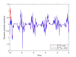
It’s easy to verify that (5.1) satisfies Assumptions 2.2. Building upon this, Theorem 3.4 states its projected Euler simulation also displays a random periodic path. To further validate this claim, we conduct numerical experiment where we observe two processes starting from $t_{0}=-10$ and $T=0$, with the stepsize of 0.01 and initial values of $0.8$ and $-0.5$. Figure 1 illustrates that two paths converge quickly, demonstrating that the random periodic solution of the projected Euler methods is independent of the initial values.

Refer to caption
Figure 1: Two paths generated by projected Euler methods from differential initial conditions

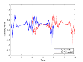
Next, we verify the periodicity by examining and dynamics under the same realisation $\omega:\tilde{X}_{t}^{-10}(\omega,0.3)$ over $-10\leq t\leq 6$ and $\tilde{X}_{t}^{-10}(\theta_{-2}\omega,0.3)$ over $-10\leq t\leq 8$, where $0.3$ is the initial condition of both processes. Due to Theorem 3.4, it is expected that $\tilde{X}^{-10}_{t}(\omega,0.3)\approx\tilde{X}^{*}_{t}(\omega)$ and $\tilde{X}^{-10}_{t}(\theta_{-2}\omega,0.3)\approx\tilde{X}^{*}_{t}(\theta_{-2}\omega)$ after a sufficiently long time, and we may then observe that $\tilde{X}^{-10}_{t-2}(\omega,0.3)\approx\tilde{X}^{-10}_{t}(\theta_{-2}\omega,0.3)$ due to the fact $\tilde{X}^{*}_{t-2}(\omega)=\tilde{X}^{*}_{t}(\theta_{-2}\omega)$ in Definition 2.1. Figure 2 demonstrates both process resemble each other with a stable time gap 2, that is, $\tilde{X}^{*}_{t-2}(\omega)=\tilde{X}^{*}_{t}(\theta_{-2}\omega)$ over $4\leq t\leq 8$.

Refer to caption
Figure 2: Simulations of the process ${\tilde{X}_{t}^{-10}(\omega,0.3),2\leq t\leq 6}$ and ${\tilde{X}_{t}^{-10}(\theta_{-2}\omega,0.3),4\leq t\leq 8}$

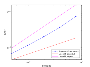
Theorem 4.2 suggests that the random periodic solution converges to the solution of (5.1) with order 0.5 in the mean square sense. To achieve this, a fine stepsize $h_{ecact}=2^{-15}\times 20$ is chosen to obtain a reference solution on the time interval $[-10,10]$. The reference solution is obtained via the same numerical method with a fine stepsize $h_{exact}=2^{-15}\times 20$. We plot mean-square approximation errors $e_{h}$ against five different stepsizes $h=2^{-i}\times 20$, $i=8,9,...,12$ on a log-log scale.

Figure 3 clearly demonstrates that the mean-square error is at a slope greater than $0.5$, but less than $1$. Suppose that the approximation error $e_{h}$ obeys a power law relation $e_{h}=Ch^{\kappa}$ for $C,\kappa>0$, so that $\log e_{h}=\log C+\kappa\log h$. Then we do a least squares power law fit for $\kappa$ and get the value 0.8544 for the rate $\kappa$ with residual of 0.1112, which is beyond the theoretical order of convergence in Theorem 4.2.

Refer to caption
Figure 3: The mean-square error plot of the projected Euler method (3.2) for simulating the solution of (5.1).

5.2 Example 2

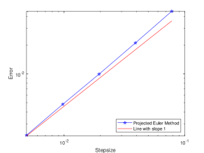
In the second example, we test the performance of the projected Euler method (3.2) with additive noise as follows:

$$\text{d}X^{t_{0}}_{t}=\Big{(}-\pi X^{t_{0}}_{t}-(X^{t_{0}}_{t})^{3}+\sin(2\pi t)\Big{)}\,\text{d}t+\text{d}W_{t}.$$ (5.2)

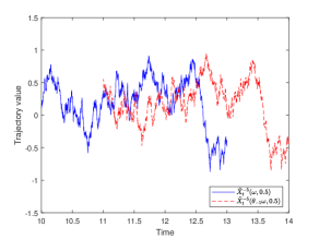
One can check that the associated period is 1 and Assumption 2.2 and 4.3 are fulfilled. We conduct a similar experiment to verify the periodicity, as described in Section 5.1. The patterns of $\tilde{X}^{-5}_{t-1}(\omega,0.5)$ over $10\leq t\leq 13$ and $\tilde{X}^{-5}_{t}(\theta_{-1}\omega,0.5)$ over $11\leq t\leq 14$ show identical results under the same realisation $\omega$ in Figure 4.

Refer to caption
Figure 4: Simulations of the processes $\tilde{X}^{-5}_{t}(\omega,0.5),10\leq t\leq 13$ and $\tilde{X}^{-5}_{t}(\theta_{-1}\omega,0.5),11\leq t\leq 14$.

The performance of the projected Euler method is also evaluated in terms of mean-square error for simulating SDE (5.2) over $[-5,15]$. The comparison between the error line and the reference line in the figure 5 indicates a close match in slopes, supporting an order-one convergence. A least squares fit yields a rate of 1.0751 with a residual of 0.0195 for (5.2). Therefore, the numerical result is in agreement with a strong order of convergence equal to one, as previously indicated in Theorem 4.5.

Refer to caption
Figure 5: The mean-square error plot of the projected Euler method (3.2) for simulating the solution of (5.2).

References

  • [1] PierreΒ M Adler and VladimirΒ V Mityushev. Resurgence flows in three-dimensional periodic porous media. Physical Review E, 82(1):016317, 2010.
  • [2] Wolf-JΓΌrgen Beyn, Elena Isaak, and Raphael Kruse. Stochastic C-stability and B-consistency of explicit and implicit Euler-type schemes. Journal of Scientific Computing, 67:955–987, 2016.
  • [3] Wolf-JΓΌrgen Beyn, Elena Isaak, and Raphael Kruse. Stochastic C-stability and B-consistency of explicit and implicit Milstein-type schemes. Journal of Scientific Computing, 70:1042–1077, 2017.
  • [4] Ziheng Chen, Liangmin Cao, and Lin Chen. Stochastic theta methods for random periodic solution of stochastic differential equations under non-globally Lipschitz conditions. arXiv preprint arXiv:2401.09747, 2024.
  • [5] Chunrong Feng, YuΒ Liu, and Huaizhong Zhao. Numerical approximation of random periodic solutions of stochastic differential equations. Zeitschrift fΓΌr angewandte Mathematik und Physik, 68(5):119, 2017.
  • [6] Chunrong Feng, Yue Wu, and Huaizhong Zhao. Anticipating random periodic solutionsβ€”i. SDEs with multiplicative linear noise. Journal of Functional Analysis, 271(2):365–417, 2016.
  • [7] Chunrong Feng and Huaizhong Zhao. Random periodic solutions of SPDEs via integral equations and Wiener–Sobolev compact embedding. Journal of Functional Analysis, 262(10):4377–4422, 2012.
  • [8] Chunrong Feng and Huaizhong Zhao. Random periodic processes, periodic measures and ergodicity. Journal of Differential Equations, 269(9):7382–7428, 2020.
  • [9] Chunrong Feng, Huaizhong Zhao, and BoΒ Zhou. Pathwise random periodic solutions of stochastic differential equations. Journal of Differential Equations, 251(1):119–149, 2011.
  • [10] Yujia Guo, Xiaojie Wang, and Yue Wu. Order-one convergence of the Backward Euler Method for Random Periodic Solutions of Semilinear SDEs. arXiv preprint arXiv:2306.06689, 2023.
  • [11] Afsaneh Moradi and Raffaele D’Ambrosio. Random periodic solutions of SDEs: Existence, uniqueness and numerical issues. Communications in Nonlinear Science and Numerical Simulation, 128:107586, 2024.
  • [12] Keiji Nakatsugawa, Toshiyuki Fujii, Avadh Saxena, and Satoshi Tanda. Time operators and time crystals: self-adjointness by topology change. Journal of Physics A: Mathematical and Theoretical, 53(2):025301, 2019.
  • [13] Chenxu Pang, Xiaojie Wang, and Yue Wu. Linear implicit approximations of invariant measures of semi-linear SDEs with non-globally lipschitz coefficients. Journal of Complexity, page 101842, 2024.
  • [14] Henri PoincarΓ©. Les mΓ©thodes nouvelles de la mΓ©canique cΓ©leste, volumeΒ 2. Gauthier-Villars et fils, imprimeurs-libraires, 1893.
  • [15] EΒ Prodan and PΒ Nordlander. On the Kohn-Sham equations with periodic background potentials. Journal of Statistical Physics, 111:967–992, 2003.
  • [16] Ata urΒ Rahman, Muhammad Khalid, SNΒ Naeem, EAΒ Elghmaz, SAΒ El-Tantawy, and LSΒ El-Sherif. Periodic and localized structures in a degenerate Thomas-Fermi plasma. Physics Letters A, 384(13):126257, 2020.
  • [17] Rong Wei and Chuanzhong Chen. Numerical Approximation of Stochastic Theta Method for Random Periodic Solution of Stochastic Differential Equations. Acta Mathematicae Applicatae Sinica, English Series, 36(3):689–701, 2020.
  • [18] Yue Wu. Backward Euler–Maruyama method for the random periodic solution of a stochastic differential equation with a monotone drift. Journal of Theoretical Probability, 36(1):605–622, 2023.
  • [19] Huaizhong Zhao and Zuohuan Zheng. Random periodic solutions of random dynamical systems. Journal of Differential Equations, 246(5):2020–2038, 2009.

Appendix A Proof of Lemma 2.3

Proof of Lemma 2.3.

Setting $y=0$ in (2.6), according to (2.11), we can have,

$$\langle x,f(t,x)\rangle+\dfrac{2p_{1}-1}{2}\|g(t,x)-g(t,0)\|^{2}\leq\alpha_{1}\|x\|^{2}+\langle x,f(t,0)\rangle,$$

then,

$$\begin{split}&\langle x,f(t,x)\rangle+\dfrac{2p_{1}-1}{2}\|g(t,x)\|^{2}\\ &\quad\leq\alpha_{1}\|x\|^{2}+\langle x,f(t,0)\rangle,+\dfrac{2p_{1}-1}{2}\langle 2g(t,x),g(t,0)\rangle+\dfrac{2p_{1}-1}{2}\|g(t,0)\|^{2}.\\ \end{split}$$

Using $2ab\leq\epsilon a^{2}+\tfrac{b^{2}}{\epsilon}$,

$$\langle x,f(t,0)\rangle\leq\tfrac{\epsilon}{2}\|x\|^{2}+\tfrac{\|f(t,0)\|^{2}}{2\epsilon},$$

similarly,

$$\begin{split}\dfrac{2p_{1}-1}{2}\langle 2g(t,x),g(t,0)\rangle&\leq\dfrac{2p_{1}-1}{2}\times\dfrac{2(p_{1}-p_{2})}{2p_{1}-1}\|g(t,x)\|^{2}+\dfrac{(2p_{1}-1)}{2}\times\dfrac{2p_{1}-1}{2(p_{1}-p_{2})}\|g(t,0)\|^{2}\\ &=\dfrac{2(p_{1}-p_{2})}{2}\|g(t,x)\|^{2}+\dfrac{(2p_{1}-1)^{2}}{4(p_{1}-p_{2})}\|g(t,0)\|^{2}.\end{split}$$

Hence,

$$\begin{split}&\langle x,f(t,x)\rangle+\dfrac{{\color[rgb]{0,0,0}2p_{2}}-1}{2}\|g(t,x)\|^{2}\\ &\quad\leq(\alpha_{1}+\epsilon)\|x\|^{2}+\dfrac{\|f(t,0)\|^{2}}{2\epsilon}+\dfrac{(2p_{1}-1)^{2}}{4(p_{1}-p_{2})}\|g(t,0)\|^{2}+\dfrac{2p_{1}-1}{2}\|g(t,0)\|^{2}.\end{split}$$

∎