Sub-Riemannian geodesics
on the Heisenberg 3D nil-manifold

Abstract

We study the projection of the left-invariant sub-Riemannian structure on the 3D Heisenberg group $G$ to the Heisenberg 3D nil-manifold $M$ — the compact homogeneous space of $G$ by the discrete Heisenberg group.

First we describe dynamical properties of the geodesic flow for $M$: periodic and dense orbits, and a dynamical characterization of the normal Hamiltonian flow of Pontryagin maximum principle. Then we obtain sharp twoside bounds of sub-Riemannian balls and distance in $G$, and on this basis we estimate the cut time for sub-Riemannian geodesics in $M$.

Keywords: Sub-Riemannian geometry, Heisenberg group, Heisenberg 3D nil-manifold, geodesics, dynamics, Hamiltonian flow, sub-Riemannian balls and distance, optimality

MSC: 53C17, 37C10, 49K15

1 Introduction

The left-invariant sub-Riemannian structure on the 3D Heisenberg group $G$ is a paradigmatic model of sub-Riemannian geometry [1, 2]. In this paper we study the projection of this sub-Riemannian structure to a compact homogeneous space of the group $G$ — to the Heisenberg 3D nil-manifold $M$. The sub-Riemannian structure on $M$ is locally isometric to the structure on $G$, thus these structures have local objects (geodesics and conjugate points) related by the projection. Although, the global issues as dynamical properties of geodesics and cut time are naturally different. We aim to study these global questions in some detail.

The structure of this work is as follows. Section 2 discusses a well known projection of Euclidean structure from $\mathbb{R}^{n}$ to the torus $\mathbb{T}^{n}$, which suggests a motivation of the subsequent study. In Sec. 3 we recall the construction of the Heisenberg 3D nil-manifold $M$. In Sec. 4 we present basic definitions of sub-Riemannian geometry, define the sub-Riemannian structures of $G$ and $M$, and describe their geodesics; in particular, we recall the parametrization of two distinct classes of sub-Riemannian geodesics in $G$ — lines and spirals. In Sec. 5 we show that sub-Riemannian geodesics-lines in $M$ may be either closed or dense, and describe explicitly geodesics falling into these classes. In Sec. 6 we describe dynamical properties of geodesics-spirals in $M$: we show that such a geodesic is either closed or dense in a certain 2D torus, and distinguish geodesics of these classes. In Sec. 7 we describe dynamical properties of the restriction of the Hamiltonian vector field for geodesics to a compact invariant surface (common level surface of the Hamiltonian and the Casimir). We show that the flow of this restriction is conjugated to a $p$-standard flow. Next in Sec. 8 we obtain sharp interior and exterior ellipsoidal bounds of sub-Riemannian balls in $G$, which improve the classical ball-box bounds. In Sec. 9 we estimate the cut time on geodesics in $M$ and the diameter of $M$ on the basis of above interior bounds of sub-Riemannian balls in $G$. Finally, in Sec. 10 we prove two-sided bounds of cut time on geodesics in $M$ on the basis of above exterior bounds of sub-Riemannian balls in $G$.

2 Motivating example

Geodesics in the Euclidean space $\mathbb{R}^{n}$ have trivial dynamics (they tend to infinity) and optimality properties (they are length minimizers).

The situation changes when we pass from $\mathbb{R}^{n}$ to its compact homogeneous space — the torus $\mathbb{T}^{n}=\mathbb{R}^{n}/\mathbb{Z}^{n}$. Consider the Riemannian structure on $\mathbb{T}^{n}$ obtained via the projection $\pi\,:\,\mathbb{R}^{n}\to\mathbb{T}^{n}$. Then the geodesics on $\mathbb{T}^{n}$ are orbits of the linear flows

$$t\mapsto(x_{1}^{0}+\omega_{1}t,\dots,x_{n}^{0}+\omega_{n}t)(\operatorname{mod}1),$$ (2.1)

$$\omega_{1}^{2}+\dots+\omega_{n}^{2}\neq 0,\qquad(x_{1}^{0},\dots,x_{n}^{0})\in\mathbb{T}^{n},\qquad t\in\mathbb{R}.$$

Kronecker’s theorem [8] (Propos. 1.5.1) states that such a geodesic is dense in $\mathbb{T}^{n}$ if and only if the frequencies $\omega_{1},\dots,\omega_{n}$ are linearly independent over $\mathbb{Q}$. In all other cases a geodesic is dense in a nontrivial $k$-dimensional torus in $\mathbb{T}^{n}$, $1\leq k<n$, see Propos. 2.1 below; in particular, a geodesic is periodic if $k=1$. See Figs. 2, 2 for $n=2$ and Figs. 4–5 for $n=3$.

The following well-known statement generalizes Kronecker’s theorem.

Proposition 2.1

(see [9, section 5.1.5]). Consider a geodesic $\Gamma$ in $\mathbb{T}^{n}$ of the form $(\ref{geodRn})$ and the corresponding vector space

$$R=\operatorname{span}_{\mathbb{Q}}\left\{r=(r_{1},\dots,r_{n})\in\mathbb{Q}^{n}\mid\sum_{i=1}^{n}r_{i}\omega_{i}=0\right\},\qquad\rho=\dim R.$$

Then $\Gamma$ is dense in a smooth manifold $S\subset\mathbb{T}^{n}$ diffeomorphic to a torus $\mathbb{T}^{n-\rho}$.

Figure 1: Geodesic $(\ref{geodRn})$ for $n=2$, $(\omega_{1},\omega_{2})=(3,2)$

Figure 2: Geodesic $(\ref{geodRn})$ for $n=2$, $(\omega_{1},\omega_{2})=(1,\sqrt{2})$

Figure 3: Geodesic $(\ref{geodRn})$ for $n=3$, $(\omega_{1},\omega_{2},\omega_{3})=(1,2,3)$

Figure 4: Geodesic $(\ref{geodRn})$ for $n=3$, $(\omega_{1},\omega_{2},\omega_{3})=(1,2,\sqrt{2})$

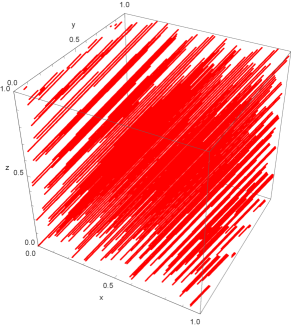
Figure 5: Geodesic $(\ref{geodRn})$ for $n=3$, $(\omega_{1},\omega_{2},\omega_{3})=(1,\sqrt{3},\sqrt{2})$

Moreover, each geodesic $(\ref{geodRn})$ loses optimality at an instant

$$t_{\operatorname{cut}}=\frac{1}{2\max|\omega_{i}|}\in(0,+\infty).$$ (2.2)

More precisely, the cut time for a geodesic $x(t)$, $t>0$, is defined as follows:

$$t_{\operatorname{cut}}(x(\cdot))=\sup\{t_{1}>0\mid x(\cdot)\text{ is length minimizing on }[0,t_{1}]\}.$$

The reason for the loss of optimality is intersection with a symmetric geodesic starting from the same initial point in $\mathbb{T}^{n}$, see Fig. 6 for the case $n=2$.

Figure 6: Optimal synthesis on $\mathbb{T}^{2}$

In this work we aim to generalize the above projection of Euclidean structure $\pi\,:\,\mathbb{R}^{n}\to\mathbb{T}^{n}$ to a projection of a left-invariant sub-Riemannian structure $\pi\,:\,G\to M$ from a Lie group $G$ to its compact homogeneous space $M$. The simplest nontrivial case of such a projection is the case of the 3D Heisenberg group $G$ and the 3D Heisenberg nil-manifold $M$, see Sec. 3.

Indeed, recall that a subgroup $H$ of a Lie group $G$ is called uniform (or cocompact) if the homogeneous space $G/H$ is compact. The only connected and simply connected non-Abelian 2D Lie group $\mathbb{R}\rtimes\mathbb{R}_{+}$ does not contain uniform subgroups. On the other hand, the 3D Heisenberg group $G$ has a countable number of uniform subgroups, of which the subgroup $(\ref{H})$ is the simplest one [12].

3 Heisenberg group and 3-dimensional nil-manifold

Recall that the Heisenberg group is

$$G=\left\{\left(\begin{matrix}1&a&c\\ 0&1&b\\ 0&0&1\end{matrix}\right)\ |\ (a,b,c)\in\mathbb{R}^{3}\right\}.$$

Consider the following discrete subgroup and its quotient (the right cosets space):

$$H=\left\{\left(\begin{matrix}1&m&k\\ 0&1&n\\ 0&0&1\end{matrix}\right)\ |\ (m,n,k)\in\mathbb{Z}^{3}\right\},\ \ \ M:={\raisebox{-1.99997pt}{$H$}\left\backslash\raisebox{1.99997pt}{$G$}\right.}=\{Hg\mid g\in G\}.$$ (3.1)

The quotient $M$ is a compact smooth manifold, which is called Heisenberg 3-dimensional nil-manifold.

Let $\pi:G\to M$ denote the canonical projection $g\mapsto Hg$. The functions

$$a^{\prime}:=\{a\},\ b^{\prime}:=\{b\},\ c^{\prime}:=\{c-[a]b\}$$

are coordinates on the homogeneous space $M$, and $\pi(a,b,c)=(a^{\prime},b^{\prime},c^{\prime})$.

Remark 3.1

The manifold $M$ is not diffeomorphic to the 3-torus $\mathbb{T}^{3}=\mathbb{R}^{3}_{a^{\prime},b^{\prime},c^{\prime}}/\mathbb{Z}^{3}$, see [5, section 5]. Indeed, the first Betti number $b_{1}$ of the torus $\mathbb{T}^{3}$ is equal to 3. On the other hand, $b_{1}(M)=2$. Indeed, the quotient projection $G\to M$ is a universal covering, since $G$ is diffeomorphic to $\mathbb{R}^{3}_{a,b,c}$. Therefore, $\pi_{1}(M)=H$. The first homology of a path connected topological space is isomorphic to the quotient of the fundamental group by its commutant, by classical Poincaré Theorem [6, section 14.3, p.181]. Hence, $H_{1}(M,\mathbb{Z})=H/[H,H]$. The commutant $[H,H]$ coincides with the subgroup of integer unipotent matrices that differ from the identity just by the upper-right corner element. Therefore, it is isomorphic to $\mathbb{Z}$. The map $H\mapsto(H_{12},H_{23})$ is an isomorphism $H/[H,H]\to\mathbb{Z}^{2}$. Therefore, $b_{1}(M)=2$.

The manifold $M$ can be represented by a fundamental domain $D=\{(a,b,c)\mid 0\leq a,b,c<1\}$ with identified facets $\{b=0\}\leftrightarrow\{b=1\}$, $\{c=0\}\leftrightarrow\{c=1\}$, while the facets $\{a=0\}$ and $\{a=1\}$ are identified by the rule $(0,b,c)\simeq(1,b,c+b)$, see Fig. 7.

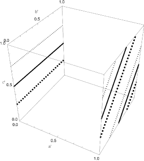
Figure 7: Heisenberg 3D nil-manifold

4 Sub-Riemannian structure on the Heisenberg group and its projection to the nil-manifold

4.1 Sub-Riemannian geometry

A sub-Riemannian structure [1, 2] on a smooth manifold $M$ is a vector subspace distribution

$$\Delta=\{\Delta_{q}\subset T_{q}M\mid q\in M\}\subset TM,\qquad\dim\Delta_{q}\equiv\operatorname{const},$$

endowed with an inner product

$$\langle\cdot,\cdot\rangle=\{\langle\cdot,\cdot\rangle_{q}\text{ inner product in }\Delta_{q}\mid q\in M\}.$$

A Lipschitzian curve $q\,:\,[0,t_{1}]\to M$ is called horizontal if $\dot{q}(t)\in\Delta_{q(t)}$ for almost all $t\in[0,t_{1}]$. The sub-Riemannian length of a horizontal curve $q(\cdot)$ is

$$l(q(\cdot))=\int_{0}^{t_{1}}\langle\dot{q}(t),\dot{q}(t)\rangle^{1/2}\,dt.$$

The sub-Riemannian distance between points $q_{0},q_{1}\in M$ is

$$d(q_{0},q_{1})=\inf\{l(q(\cdot))\mid q(\cdot)\text{ horiz. curve s.t. }q(0)=q_{0},\ q(t_{1})=q_{1}\}.$$

A horizontal curve is called a sub-Riemannian length minimizer if its sub-Riemannian length is equal to the sub-Riemannian distance between its endpoints. A sub-Riemannian geodesic is a horizontal curve whose sufficiently short arcs are length minimizers. Finally, a cut time along a sub-Riemannian geodesic $q(\cdot)$ is

$$t_{\operatorname{cut}}(q(\cdot))=\sup\{\tau>0\mid\left.q(\cdot)\right|_{[0,\tau]}\text{ is a length minimizer}\}.$$

If the distribution $\Delta$ is completely nonholonomic (completely nonintegrable), i.e., any points in $M$ can be connected by a horizontal curve of $\Delta$, then the sub-Riemannian distance $d$ turns $M$ into a metric space, and there are naturally defined a sub-Riemannian sphere of radius $R\geq 0$ centered at a point $q_{0}\in M$:

$$S_{R}(q_{0})=\{q\in M\mid d(q_{0},q)=R\}$$

and the corresponding sub-Riemannian ball:

$$B_{R}(q_{0})=\{q\in M\mid d(q_{0},q)\leq R\}.$$

Let $X_{1},\dots X_{k}$ be vector fields on $M$ that form an orthonormal frame of a sub-Riemannian structure $(\Delta,\langle\cdot,\cdot\rangle)$:

$$\Delta_{q}=\operatorname{span}(X_{1}(q),\dots,X_{k}(q)),\quad\langle X_{i}(q),X_{j}(q)\rangle=\delta_{ij},\qquad q\in M.$$

Then sub-Riemannian length minimizers that connect points $q_{0},q_{1}\in M$ are solutions to the optimal control problem

$$\dot{q}=\sum_{i=1}^{k}u_{i}(t)X_{i}(q),\qquad q\in M,\quad u=(u_{1},\dots,u_{k})\in\mathbb{R}^{k},$$

$$q(0)=q_{0},\qquad q(t_{1})=q_{1},$$

$$\int^{t_{1}}_{0}\left(\sum_{i=1}^{k}u^{2}_{i}(t)\right)^{1/2}\,dt\to\min.$$

4.2 Sub-Riemannian structures on $G$ and $M$

The left-invariant sub-Riemannian problem on the Heisenberg group is stated as the following optimal control problem [2, 3, 10]:

$$\dot{g}=u_{1}(t)X_{1}(g)+u_{2}(t)X_{2}(g),\qquad g\in G,\quad u=(u_{1},u_{2})\in\mathbb{R}^{2},$$ (4.1)

$$g(0)=g_{0}=\operatorname{Id},\qquad g(t_{1})=g_{1},$$ (4.2)

$$\int^{t_{1}}_{0}(u^{2}_{1}(t)+u^{2}_{2}(t))^{1/2}\,dt\to\min,$$ (4.3)

$$X_{1}=\frac{\partial}{\partial x}-\frac{y}{2}\frac{\partial}{\partial z},\quad X_{2}=\frac{\partial}{\partial y}+\frac{x}{2}\frac{\partial}{\partial z}.$$ (4.4)

The fields $X_{1}$, $X_{2}$ are left-invariant vector fields on $G$.

Here and below we use coordinates $(x,y,z)$ on the Heisenberg group $G$ such that

$$a=x,\quad b=y,\quad c=z+\frac{xy}{2}.$$ (4.5)

Geodesics for this problem have the form:

$$x=t\cos\theta,$$ (4.6)

$$y=t\sin\theta,$$ (4.7)

$$z=0$$ (4.8)

for $\theta\in\mathbb{R}/(2\pi\mathbb{Z})$, and

$$x=(\sin(\theta+ht)-\sin\theta)/h,$$ (4.9)

$$y=(\cos\theta-\cos(\theta+ht))/h,$$ (4.10)

$$z=(ht-\sin ht)/(2h^{2})$$ (4.11)

for $\theta\in\mathbb{R}/(2\pi\mathbb{Z})$ and $h\neq 0$.

Sub-Riemannian geodesics (4.6)–(4.8) are one-parametric subgroups in $G$, they are projected to the plane $(x,y)$ into straight lines, thus we call them geodesics-lines in the sequel. Sub-Riemannian geodesics (4.9)–(4.11) are spirals of nonconstant slope in $\mathbb{R}_{x,y,z}^{3}\simeq G$, they are projected to the plane $(x,y)$ into circles, and we call them geodesics-spirals in the sequel.

Sub-Riemannian problem (4.1)–(4.4) is left-invariant on the Heisenberg group $G$, thus its projection to the nil-manifold $M$ is a well-defined sub-Riemannian problem on $M$:

$$\dot{g^{\prime}}=u_{1}X_{1}^{\prime}(g^{\prime})+u_{2}X_{2}^{\prime}(g^{\prime}),\qquad g^{\prime}\in M,\quad u=(u_{1},u_{2})\in\mathbb{R}^{2},$$ (4.12)

$$g^{\prime}(0)=g_{0}^{\prime}=\pi(\operatorname{Id}),\qquad g^{\prime}(t_{1})=g_{1}^{\prime},$$ (4.13)

$$\int^{t_{1}}_{0}(u^{2}_{1}+u^{2}_{2})^{1/2}\,dt\to\min,$$ (4.14)

$$X_{i}^{\prime}(g^{\prime})=\pi_{*}(X_{i}(g)),\qquad g^{\prime}=\pi(g),\qquad i=1,2,\quad g\in G.$$ (4.15)

Geodesics of the projected problem (4.12)–(4.15) have the form $g^{\prime}(t)=\pi(g(t))$, where $g(t)$ are geodesics of the initial problem (4.1)–(4.4).

5 Projections of geodesics-lines
to Heisenberg nil-manifold

For every $\theta\in\mathbb{R}/(2\pi\mathbb{Z})$ consider a geodesic-line (4.6)–(4.8) in $G$ and its projection to $M$:

$$g(t)=(a(t),b(t),c(t))=\left(t\cos\theta,t\sin\theta,\frac{t^{2}}{2}\sin\theta\cos\theta\right),\ \ t\in\mathbb{R}.$$

$$g^{\prime}(t):=\pi\circ g(t)=(a^{\prime}(t),b^{\prime}(t),c^{\prime}(t)),$$

$$a^{\prime}(t)=\{t\cos\theta\},\ b^{\prime}(t)=\{t\sin\theta\},\ c^{\prime}(t)=\left\{\frac{t^{2}}{2}\sin\theta\cos\theta-[t\cos\theta]t\sin\theta\right\},$$ (5.1)

$$\Gamma:=\{g^{\prime}(t)\ |\ t\in\mathbb{R}\}\subset M.$$

Consider the projection $\rho:M\to\mathbb{T}^{2}=\mathbb{R}^{2}/\mathbb{Z}^{2}$ and the image $\rho(\Gamma)$:

$$\rho:(a^{\prime},b^{\prime},c^{\prime})\mapsto(a^{\prime},b^{\prime}),\ \ \gamma:=\rho(\Gamma)=\{(a^{\prime}(t),b^{\prime}(t))\ |\ t\in\mathbb{R}\}\subset\mathbb{T}^{2}.$$

Remark 5.1

If $\theta=\frac{\pi n}{2}$, $n\in\mathbb{Z}$, then $\gamma$ and $\Gamma$ are both 1-periodic. If $\tan\theta\in\mathbb{Q}\setminus\{0\}$, then $\gamma$ is periodic, and $\rho^{-1}(\gamma)$ is a two-dimensional torus.

Proposition 5.2

If $\tan\theta=\frac{p}{q}\in\mathbb{Q}\setminus\{0\}$, then the curve $\gamma$ is periodic with period $T=\frac{q}{\cos\theta}$; here $(p,q)=1$. The curve $\Gamma$ is periodic either with the same period, as $\gamma$, if some of the numbers $p$, $q$ is even, or with twice bigger period otherwise.

See Figs. 9, 9.

Figure 8: The curve $\gamma$ for $\tan\theta=3$

Figure 9: The curve $\Gamma$ for $\tan\theta=3$

Proof.

One has

$$T\cos\theta=q\in\mathbb{Z},\ \ T\sin\theta=p\in\mathbb{Z},$$ (5.2)

$$(a(t+T),b(t+T)=(a(t)+q,b(t)+p).$$

This implies $T$-periodicity of the curve $\gamma$. One has

$$c^{\prime}(t+T)=\{c(t+T)-[a(t+T)]b(t+T)\}$$

$$=\left\{\frac{(t+T)^{2}}{2}\sin\theta\cos\theta-[(t+T)\cos\theta](t+T)\sin\theta\right\}$$

$$=\left\{\frac{t^{2}}{2}\sin\theta\cos\theta+tT\sin\theta\cos\theta+\frac{T^{2}}{2}\sin\theta\cos\theta-[(t+T)\cos\theta](t+T)\sin\theta\right\}.$$

Substituting (5.2) yields

$$c^{\prime}(t+T)=\left\{\frac{t^{2}}{2}\sin\theta\cos\theta+tq\sin\theta+\frac{pq}{2}-[t\cos\theta+q](t\sin\theta+p)\right\}$$

$$=\left\{\frac{t^{2}}{2}\sin\theta\cos\theta+tq\sin\theta+\frac{pq}{2}-([t\cos\theta]+q)(t\sin\theta+p)\right\}$$

$$=\left\{\frac{t^{2}}{2}\sin\theta\cos\theta+tq\sin\theta+\frac{pq}{2}-[t\cos\theta]t\sin\theta-qt\sin\theta-p[t\cos\theta]-pq\right\}$$

$$=\left\{\frac{t^{2}}{2}\sin\theta\cos\theta-[t\cos\theta]t\sin\theta-\frac{pq}{2}\right\}.$$

The latter expression is equal to either $c^{\prime}(t)$, if $pq$ is even, or $\{c^{\prime}(t)+\frac{1}{2}\}$ otherwise. In the latter case replacing $T$ by $2T$ and repeating the above argument with $q$, $p$ replaced by $2q$, $2p$ yields $c^{\prime}(t+2T)=c^{\prime}(t)$. The proposition is proved. ∎

Theorem 5.3

The curve $\Gamma$ is dense in $M$ for every $\theta\in\mathbb{R}$ such that $\tan\theta\notin\mathbb{Q}\cup\{\infty\}$. In this case each its half  $\Gamma_{\pm}=\{g^{\prime}(t)\ |\ t\in\mathbb{R}_{\pm}\}$ is dense.

See Figs. 11, 11.

Figure 10: The curve $\gamma$ for $\tan\theta=\sqrt{2}$

Figure 11: The curve $\Gamma$ for $\tan\theta=\sqrt{2}$

As it is shown below, Theorem 5.3 is implied by the following theorem.

Theorem 5.4

The sequence $\{(\{2rn\},\{rn^{2}\})\in\mathbb{T}^{2}\ |\ n\in\mathbb{N}\}$ is dense in $\mathbb{T}^{2}$ for every $r\in\mathbb{R}\setminus\mathbb{Q}$.

Theorem 5.4 follows from a more general result due to H.Furstenberg, see [7, lemma 2.1], which yields unique ergodicity of the torus map (5.6). Below we present a proof of Theorem 5.4 for completeness of presentation.

Remark 5.5

It is known that for every real polynomial $P(n)=\alpha_{0}n^{m}+\alpha_{1}n^{m-1}+\dots+\alpha_{m}$ with $\alpha_{0}\notin\mathbb{Q}$ the values $P(n)$ are equidistributed (thus, dense) on the segment $[0,1]$ (Furstenberg’s theorem, see [8, exercise 4.2.7]). This theorem also follows from the above-mentioned Furstenberg’s result on unique ergodicity of map (5.6).

Proof.

of Theorem 5.3 modulo Theorem 5.4. We prove the statement of Theorem 5.3 for the half-curve $\Gamma_{+}$; the proof for $\Gamma_{-}$ is analogous.

Let us do the above calculation with

$$T=\frac{q}{\cos\theta},\ \ q\in\mathbb{Z}_{\geq 0}:$$

$$T\cos\theta=q\in\mathbb{Z}_{\geq 0},\ \ T\sin\theta=q\tan\theta,$$

$$c^{\prime}(t+T)=\{c(t+T)-[a(t+T)]b(t+T)\}$$

$$=\left\{\frac{(t+T)^{2}}{2}\sin\theta\cos\theta-[(t+T)\cos\theta](t+T)\sin\theta\right\}$$

$$=\left\{\frac{t^{2}}{2}\sin\theta\cos\theta+tT\sin\theta\cos\theta+\frac{T^{2}}{2}\sin\theta\cos\theta-[(t+T)\cos\theta](t+T)\sin\theta\right\}$$

$$=\left\{\frac{t^{2}}{2}\sin\theta\cos\theta+tq\sin\theta+\frac{q^{2}\tan\theta}{2}-([t\cos\theta]+q)(t\sin\theta+q\tan\theta)\right\}$$

$$=c^{\prime}_{q}(t):=\left\{\frac{t^{2}}{2}\sin\theta\cos\theta-[t\cos\theta]t\sin\theta-[t\cos\theta]q\tan\theta-q^{2}\frac{\tan\theta}{2}\right\}.$$ (5.3)

Set

$$\widehat{\Gamma}_{q}:=\{\Gamma(t+\frac{q}{\cos\theta})\ |\ t\in[0,\frac{1}{\cos\theta})\}\ \ \text{ for every }\ q\in\mathbb{Z}_{\geq 0}.$$

By definition,

$$\Gamma_{+}\cup\{g^{\prime}(0)\}=\cup_{q\in\mathbb{Z}_{\geq 0}}\widehat{\Gamma}_{q}.$$ (5.4)

Set

$$r=\frac{\tan\theta}{2}.$$

Each curve $\widehat{\Gamma}_{q}$ admits the coordinate representation

$$\widehat{\Gamma}_{q}(t)=(a^{\prime}(t),\{b^{\prime}(t)+2qr\},\{c^{\prime}(t)-rq^{2}\}),$$ (5.5)

since for every $t\in[0,\frac{1}{\cos\theta})$ one has

$$c^{\prime}_{q}(t)=\left\{\frac{t^{2}}{2}\sin\theta\cos\theta-[t\cos\theta]t\sin\theta-q^{2}\frac{\tan\theta}{2}\right\}=\{c^{\prime}(t)-rq^{2}\}:$$

$[t\cos\theta]=0$, whenever $t\in[0,\frac{1}{\cos\theta})$. For every $t$ the sequence $(\{b^{\prime}(t)+2qr\},\{c^{\prime}(t)-rq^{2}\})$ is dense in $[0,1)\times[0,1)$. To prove this, it suffices to show that the sequence $(\{2qr\},\{-rq^{2}\})$ is dense in $[0,1)\times[0,1)$. Or equivalently, density of the projection to $\mathbb{T}^{2}=\mathbb{R}^{2}/\mathbb{Z}^{2}$ of the sequence $(2qr,-rq^{2})$. Indeed, the projection to $\mathbb{T}^{2}$ of the sequence $(2qr,rq^{2})$ is dense, by Theorem 5.4. The sequence $(2qr,-rq^{2})$ is obtained from the latter sequence with dense projection by the symmetry $(x,y)\mapsto(x,-y)$, which is the lifting to $\mathbb{R}^{2}$ of torus automorphism given by the same formula. Every torus automorphism sends any dense subset to a dense subset. The latter symmetry sends the projection of the sequence $(2qr,rq^{2})$ to the projection of the sequence $(2qr,-rq^{2})$. Therefore, the latter projection is dense. Hence, the sequence $(\{b^{\prime}(t)+2qr\},\{c^{\prime}(t)-rq^{2}\})$ is dense in $[0,1)\times[0,1)$ for every $t\in[0,\frac{1}{\cos\theta})$. This together with (5.5) and (5.4) implies density of the curve $\Gamma_{+}$ in $M$. ∎

For the proof of Theorem 5.4 let us introduce the torus map

$$T:\mathbb{T}^{2}\to\mathbb{T}^{2},\ T(x,y)=(x+\alpha,y+x+\beta).$$ (5.6)

Proposition 5.6

Set $\alpha=2r$, $\beta=r$. Then

$$(\{2rn\},\{rn^{2}\})=T^{n}(0,0).$$ (5.7)

Proof.

Induction in $n$.

Induction base: for $n=1$ one has $T(0,0)=(2r,r)(\operatorname{mod}\mathbb{Z}^{2})$.

Induction step. Let $T^{n}(0,0)=(2rn,rn^{2})(\operatorname{mod}\mathbb{Z}^{2})$. Then modulo $\mathbb{Z}^{2}$,

$$T^{n+1}(0,0)=(2r(n+1),rn^{2}+2rn+r)=(2r(n+1),r(n+1)^{2}).$$

The induction step is done. The proposition is proved. ∎

Theorem 5.7

For every $\alpha\in\mathbb{R}\setminus\mathbb{Q}$ and every $\beta\in\mathbb{R}$ the map $T$ given by (5.6) is minimal: each its forward orbit is dense.

Proof.

Suppose the contrary: there exists a point $(x_{0},y_{0})$ with non-dense forward orbit. Let $M$ denote the set of limit points of its orbit. (The orbit is non-periodic, as is the rotation $x\mapsto x+\alpha$.) The set $M$ is a non-empty closed subset in $\mathbb{T}^{2}$ with a non-empty open complement

$$V:=\mathbb{T}^{2}\setminus M.$$

Remark 5.8

The set $M$ is $T$- and $T^{-1}$-invariant, hence so is $V$.

Proposition 5.9

The set $V$ contains no fiber $z\times S^{1}$.

Proof.

Suppose the contrary: $V$ contains such a fiber. Then there exists an interval neighborhood $U=U(z)\subset S^{1}$ such that $U\times S^{1}\subset V$. But the successive images $T^{m}(U\times S^{1})$ cover all of $\mathbb{T}^{2}$: the images of the interval $U$ by translations $x\mapsto x+m\alpha$ cover all of $S^{1}$, since $\alpha$ is irrational. Therefore, $V=\mathbb{T}^{2}$. The contradiction thus obtained proves the proposition. ∎

Fix $a,b,c,d\in[0,1)$, $a<b$, $c<d$, such that

$$\Pi:=[a,b]\times[c,d]\subset V.$$

Set

$$h:=d-c.$$

Proposition 5.10

For every $k\in\mathbb{Z}_{\geq 0}$ there exists a fiber $S^{1}_{k}=z_{k}\times S^{1}$ such that $S^{1}_{k}\cap V$ contains an arc of length greater than $2^{k}h$. In the case, when $2^{k}h>1$, this means that the whole fiber $S^{1}_{k}$ lies in $V$.

Proof.

The proof is based on area-preserving property of the map $T$ and the fact that for every $N\in\mathbb{N}$ the iterate $T^{N}$ lifted to $\mathbb{R}^{2}$ transforms horizontal lines to lines with the slope (the tangent of angle with the horizontal axis) equal to $N$. Thus, as $N\to\infty$, the images of horizontal lines tend to vertical lines. Therefore, the images of a rectangle become very long strips spiralling in nearly vertical direction.

Induction in $k$.

Induction base for $k=0$. Each fiber $z\times S^{1}$, $z\in[a,b]$, intersects $V$ by an arc strictly containing the arc $z\times[c,d]$ of length $h$, and thus, having a bigger length.

Induction step. Let there exist a $z_{k}\in S^{1}$ such that the intersection $(z_{k}\times S^{1})\cap V$ contains a segment $z_{k}\times[c_{k},d_{k}]$ of length $c_{k}-d_{k}>2^{k}h$. Let us show that $V$ contains a vertical circle arc of twice bigger length. To do this, fix an $\varepsilon>0$ such that

$$\Pi_{k}:=[z_{k}-3\varepsilon,z_{k}+3\varepsilon]\times[c_{k},d_{k}]\subset V.$$

Fix a $\delta\in(0,\varepsilon)$ such that $2\delta<h$. For every $N\in\mathbb{N}$ there exists a point

$$(x_{N},y_{N})\in\Pi_{k,\delta}:=[z_{k}-\varepsilon,z_{k}+\varepsilon]\times[c_{k},c_{k}+\delta]\subset\Pi_{k}$$

such that

$$p_{n}:=T^{n}(x_{N},y_{N})\in\Pi_{k,\delta}\text{ for some }n>N,$$

by area-preserving property and the Poincaré Recurrence Theorem [8, theorem 4.1.19].

Claim 1. Let us choose $N>\frac{d_{k}-c_{k}+2\delta}{\varepsilon}$. Let $(x_{N},y_{N})$ and $n$ be as above. Then the $T^{n}$-image of the lower horizontal side $L:=[z_{k}-3\varepsilon,z_{k}+3\varepsilon]\times c_{k}$ of the rectangle $\Pi_{k}$ intersects its upper side at some point $q_{k}$. See Fig.12.

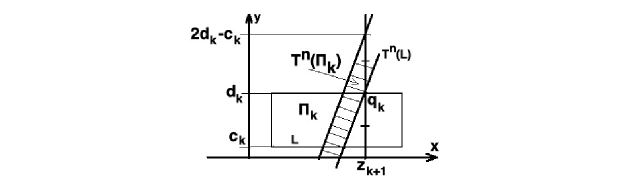
Figure 12: The rectangle $\Pi_{k}$, its image $T^{n}(\Pi_{k})$ and the intersection point $q_{k}$.

Proof.

The point $(x_{N},c_{k})$ lies in the lower side $L$, $|x_{N}-z_{k}|\leq\varepsilon$, and $0\leq y_{N}-c_{k}\leq\delta$. The $y$-coordinate of its image, $y_{n}:=y(T^{n}(x_{N},c_{k}))$ also differs from $c_{k}$ by a quantity no greater than $\delta$, since it is no greater than that $y_{n}^{\prime}:=y(T^{n}(x_{N},y_{N}))\in[c_{k},c_{k}+\delta]$, $y^{\prime}_{n}-y_{n}=y_{N}-c_{k}\in[0,\delta]$: the map $T$ preserves the lengths of arcs of vertical fibers. The $x$-coordinate of the same image $T^{n}(x_{N},c_{k})$ lies in the segment $[z_{k}-\varepsilon,z_{k}+\varepsilon]$. This together with the inequality on $N$ and the fact that the $T^{n}$-image of a horizontal segment has slope $n>N$ implies that $T^{n}(L)$ crosses the upper side of the rectangle $\Pi_{k}$. ∎

Let $q_{k}=(z_{k+1},d_{k})=T^{n}(p_{k})$ be a point of the above crossing, $p_{k}=(s_{k},c_{k})\in L$. Then $s_{k}\times[c_{k},d_{k}]\subset\Pi_{k}\subset V$, by assumption. Therefore, $z_{k+1}\times[d_{k},d_{k}+(d_{k}-c_{k})]=T^{n}(s_{k}\times[c_{k},d_{k}])\subset V$, by invariance of the set $V$. Finally, the vertical circle arc $z_{k+1}\times[c_{k},2d_{k}-c_{k}]$ of length $2(d_{k}-c_{k})>2^{k+1}h$ lies in $V$. The induction step is done. Proposition 5.10 is proved. ∎

Proposition 5.10 applied to $k$ large enough implies that $V$ contains a vertical fiber $z\times S^{1}$. This contradicts Proposition 5.9. Theorem 5.7 is proved. ∎

Theorem 5.7 implies Theorem 5.4, and hence, Theorem 5.3.

6 Projections of geodesics-spirals
to Heisenberg nil-manifold

For every $\theta\in\mathbb{R}/(2\pi\mathbb{Z})$, $h\neq 0$ consider a geodesic-spiral (4.9)–(4.11) in $G$ and its projection to $M$:

$$a(t)=(\sin(\theta+ht)-\sin\theta)/h,$$

$$b(t)=(\cos\theta-\cos(\theta+ht))/h,$$

$$c(t)=(ht-\sin ht)/(2h^{2})+a(t)b(t)/2,$$

$$g(t)=(a(t),b(t),c(t)),\ \ t\in\mathbb{R}.$$

$$g^{\prime}(t):=\pi\circ g(t)=(a^{\prime}(t),b^{\prime}(t),c^{\prime}(t)),$$

$$\Gamma:=\{g^{\prime}(t)\ |\ t\in\mathbb{R}\}\subset M.$$

The projection $G\to\mathbb{R}\times\mathbb{R}$, $(a,b,c)\mapsto(a,b)$ passes to the quotient and induces the projection

$$p:M\to\mathbb{T}^{2}=S^{1}\times S^{1},\ \ S^{1}=\mathbb{R}/\mathbb{Z}.$$

Theorem 6.1

1) The projection $p$ sends each geodesic-spiral $\Gamma$, see (4.9)–(4.11), to a contractible closed curve $\gamma\subset\mathbb{T}^{2}$ that may have self-intersections.

2) The geodesic-spiral $\Gamma$ is

- either closed, which holds if and only if $h^{2}\in\pi\mathbb{Q}\setminus\{0\}$;

- or dense in the preimage $p^{-1}(\gamma)\subset M$, if $h^{2}\notin\pi\mathbb{Q}$.

See Figs. 14–16.

Figure 13: The curve $\gamma$ for $h=\sqrt{\pi/2}$

Figure 14: The curve $\Gamma$ for $h=\sqrt{\pi/2}$

Figure 15: The curve $\gamma$ for $h=1$

Figure 16: The curve $\Gamma$ for $h=1$

Proof.

The projection $p(\Gamma)\subset\mathbb{T}^{2}$ of the spiral geodesic $\Gamma$ given by (4.9)–(4.11) is $\frac{2\pi}{h}$-periodic in $t$, as are the right-hand sides in (4.9) and (4.10). Therefore, it is a closed curve. Statement 1) is proved.

The coordinate $c^{\prime}=\{c-[a]b\}$ of a point of the geodesic $\Gamma$ is equal to

$$c^{\prime}(t)=\left\{\frac{t}{2h}-\frac{\sin ht}{2h^{2}}+\frac{x(t)y(t)}{2}-[x(t)]y(t)\right\},$$ (6.1)

where $x(t)$, $y(t)$ are given by (4.9) and (4.10) respectively. All the terms in the right-hand side in (6.1) except for the first one are $\frac{2\pi}{h}$-periodic functions in $t$. Adding $\frac{2\pi}{h}$ to $t$ results in adding $\frac{\pi}{h^{2}}$ to the first term $\frac{t}{2h}$. Therefore, closeness of the geodesic $\Gamma$ is equivalent to commensurability of the numbers $h^{2}$ and $\pi$. If they are incommensurable, then the sequence of the numbers $\{\frac{\pi n}{h^{2}}\}$ with $n\in\mathbb{N}$ is dense in $[0,1]$. This together with the above discussion implies that $\Gamma$ is dense in $p^{-1}(\gamma)$. The theorem is proved. ∎

7 Dynamics of the normal Hamiltonian flow
on $T^{*}M$

Let $T^{*}M$ be the cotangent bundle of the Heisenberg nil-manifold $M$. Introduce linear on fibers of $T^{*}M$ Hamiltonians $h_{i}(\lambda)=\langle\lambda,X_{i}^{\prime}\rangle$, $i=1,2,3$, where $X_{3}^{\prime}=[X_{1}^{\prime},X_{2}^{\prime}]=\frac{\partial}{\partial z^{\prime}}$.

Let $H(\lambda)=(h_{1}^{2}(\lambda)+h_{2}^{2}(\lambda))/2$ be the normal Hamiltonian of Pontryagin maximum principle [2, 10] for the sub-Riemannian problem (4.12)–(4.15), and let $\vec{H}$ be the corresponding Hamiltonian vector field on $T^{*}M$. Sub-Riemannian geodesics on $M$ are projections of trajectories of the normal Hamiltonian system

$$\dot{\lambda}=\vec{H}(\lambda),\qquad\lambda\in T^{*}M,$$ (7.1)

in coordinates

$$\dot{h}_{1}=-h_{2}h_{3},\quad\dot{h}_{2}=h_{1}h_{3},\quad\dot{h}_{3}=0,\quad\dot{g}^{\prime}=h_{1}X_{1}^{\prime}+h_{2}X_{2}^{\prime},$$ (7.2)

this follows from the classical coordinate expression of the Hamiltonian system for sub-Riemannian geodesics on the Heisenberg group [2, 10]. Hamiltonian system (7.2) has integrals $H$ and $h_{3}$, thus each level surface

$$S_{p}=\{\lambda\in T^{*}M\mid H(\lambda)=1/2,\ h_{3}(\lambda)=p\},\qquad p\in\mathbb{R},$$

is invariant for the field $\vec{H}$. Denote on this level surface $h_{1}=\cos\theta$, $h_{2}=\sin\theta$. Denote also the restriction $V_{p}=\left.\vec{H}\right|_{S_{p}}$. The ODE

$$\dot{\lambda}=V_{p}(\lambda),\qquad\lambda\in S_{p},$$ (7.3)

reads in coordinates as

$$\begin{cases}\dot{\theta}=p,\\ \dot{a}^{\prime}=\cos\theta,\\ \dot{b}^{\prime}=\sin\theta,\\ \dot{c}^{\prime}=a^{\prime}\sin\theta,\end{cases}$$ (7.4)

this follows immediately from ODEs $(\ref{dh1})$ via the transformation formulas $(\ref{abcxyz})$.

Set

$$S^{1}_{\nu}:=\mathbb{R}_{\nu}/\mathbb{Z}\ \ \ \text{ for }\nu=a,b,c;\ \ S^{1}_{\theta}=\mathbb{R}_{\theta}/2\pi\mathbb{Z}.$$

Let us introduce yet another flow on $S_{p}=S^{1}_{\theta}\times M$.

Definition 7.1

The $p$-standard flow $F^{t}_{p}$ on $S^{1}_{\theta}\times M$ is given in the coordinates by the equation

$$\begin{cases}\dot{\theta}=p,\\ \dot{a}^{\prime}=0,\\ \dot{b}^{\prime}=0,\\ \dot{c}^{\prime}=\frac{1}{2p}.\end{cases}$$ (7.5)

Remark 7.2

The projection of the vector field given by (7.5) to the 2-torus $\mathbb{T}^{2}_{\theta,c^{\prime}}$ is the linear vector field $\dot{\theta}=p$, $\dot{c}^{\prime}=\frac{1}{2p}$. Its flow map in time $\frac{2\pi}{p}$ fixes each circle $\{\theta\}\times S^{1}_{c^{\prime}}$ and acts on it by translation (rotation)

$$c^{\prime}\mapsto c^{\prime}+\rho,\ \ \ \ \ \rho:=\frac{\pi}{p^{2}}.$$

The number $\rho$ is its rotation number, see the definition of rotation number in [4, p. 104].

Theorem 7.3

Flow (7.3) is conjugated to the $p$-standard flow by a diffeomorphism of $S_{p}=S^{1}_{\theta}\times M$ preserving the $\theta$-coordinate and isotopic to the identity in the class of diffeomorphisms preserving the $\theta$-coordinate.

Remark 7.4

Let $\pi:G\to M$ denote the quotient projection. Consider the pullbacks to $S^{1}_{\theta}\times G$ of vector fields (7.4), (7.5) under the induced projection $S^{1}\times G\to S^{1}\times M$. The pullbacks are written by the same formulas, as (7.4), (7.5), but in the coordinates $(\theta,a,b,c)$.

For the proof of Theorem 7.3 we first solve equations (7.4) and show that their solutions are all $\frac{2\pi}{p}$-periodic, except for the function $c(t)$, which is equal to $\frac{t}{2p}$ plus a $\frac{2\pi}{p}$-periodic function. Using formulas for solutions, we construct an explicit analytic family of diffeomorphisms $F_{\nu}:S^{1}_{\theta}\times G\to S^{1}_{\theta}\times G$ preserving the $\theta$-coordinate, depending on the parameter $\nu\in[0,1]$, $F_{0}=\operatorname{Id},$ such that $F_{1}$ transforms the lifted vector field (7.4) to the lifted field (7.5), see the above remark. We show that each $F_{\nu}$ is $\Gamma$-equivariant and thus, the family $F_{\nu}$ induces a family of diffeomorphisms $S^{1}\times M\to S^{1}\times M$ with $F_{1}$ sending (7.4) to (7.5). This will prove Theorem 7.3.

Proposition 7.5

Each solution of the differential equation defined by the lifted vector field (7.4) (thus, written in the coordinates $(\theta,a,b,c)$) with initial condition $(\theta_{0},a_{0},b_{0},c_{0})$ at $t=0$ takes the form

$$\begin{cases}\theta(t)=\theta_{0}+pt\\ a(t)=\frac{1}{p}(\sin(\theta_{0}+pt)-\sin\theta_{0})+a_{0}\\ b(t)=\frac{1}{p}(\cos\theta_{0}-\cos(\theta_{0}+pt))+b_{0}\\ c(t)=\frac{t}{2p}-\frac{1}{4p^{2}}(\sin 2(\theta_{0}+pt)+\sin 2\theta_{0})+\frac{1}{2p^{2}}(\sin(2\theta_{0}+pt)-\sin pt)\\ -\frac{a_{0}}{p}(\cos(\theta_{0}+pt)-\cos\theta_{0})+c_{0}.\end{cases}$$ (7.6)

Proof.

The three first equations in (7.4) are solved by direct integration. The fourth equation is solved by taking the primitive:

$$c(t)=c_{0}+\int_{0}^{t}a(t)\sin\theta(t)dt$$

$$=c_{0}+\int_{0}^{t}(\frac{1}{p}(\sin(\theta_{0}+pt)-\sin\theta_{0})+a_{0})\sin(\theta_{0}+pt)dt.$$ (7.7)

The latter subintegral expression is equal to

$$\frac{1}{2p}(1-\cos 2(\theta_{0}+pt)+\cos(2\theta_{0}+pt)-\cos pt)+a_{0}\sin(\theta_{0}+pt).$$

Therefore, the integral is equal to

$$\frac{t}{2p}-\frac{1}{4p^{2}}(\sin 2(\theta_{0}+pt)-\sin 2\theta_{0}+2\sin 2\theta_{0}-2\sin(2\theta_{0}+pt)+2\sin pt)$$

$$+\frac{a_{0}}{p}(\cos\theta_{0}-\cos(\theta_{0}+pt)).$$

This together with (7.7) yields (7.6). ∎

Proposition 7.6

The phase curves of the lifted vector field (7.4) are graphs of vector functions $(a(\theta),b(\theta),c(\theta))$, where

$$\begin{cases}a(\theta)=\frac{\sin\theta}{p}+a_{0}\\ b(\theta)=\frac{1}{p}(1-\cos\theta)+b_{0}\\ c(\theta)=\frac{\theta}{2p^{2}}-\frac{1}{4p^{2}}\sin 2\theta-\frac{a_{0}}{p}(\cos\theta-1)+c_{0},\end{cases}$$ (7.8)

$$a_{0}=a(0),b_{0}=b(0),c_{0}=c(0).$$

Proof.

Each phase curve intersects the fiber $\{\theta=0\}$. Hence, it is the graph of a solution (7.6) with $\theta_{0}=0$. Substituting $\theta_{0}=0$ to (7.6) yields

$$\begin{cases}\theta(t)=pt\\ a(t)=\frac{\sin\theta}{p}+a_{0}\\ b(t)=\frac{1}{p}(1-\cos\theta)+b_{0}\\ c(t)=\frac{t}{2p}-\frac{1}{4p^{2}}\sin 2\theta-\frac{a_{0}}{p}(\cos\theta-1)+c_{0},\end{cases}$$

which implies (7.8). ∎

Consider the following family of diffeomorphisms $F_{\nu}:S^{1}_{\theta}\times G\to S^{1}_{\theta}\times G$:

$$F_{\nu}(\theta,a,b,c)=(\theta,\ a-\frac{\nu}{p}\sin\theta,\ b-\frac{\nu}{p}(1-\cos\theta),\ \widetilde{c}_{\nu}),$$

$$\widetilde{c}_{\nu}:=c+\nu\left(\frac{1}{4p^{2}}\sin 2\theta+\frac{1}{p}(a-\frac{\sin\theta}{p})(\cos\theta-1)\right),\ \nu\in[0,1].$$ (7.9)

The action of the group $\Gamma$ on $G$ by left multiplication lifts to its action on $S^{1}_{\theta}\times G$:

$$\gamma(\theta,g):=(\theta,\gamma g)\ \text{ for every }\ \gamma\in\Gamma,\ g\in G.$$

Proposition 7.7

1) For every $\nu\in\mathbb{R}$ the map $F_{\nu}$ is a diffeomorphism equivariant under left multiplications by elements of the group $\Gamma$:

$$F_{\nu}(\theta,\gamma g)=\gamma F_{\nu}(\theta,g)\text{ for every }\gamma\in\Gamma,\ g\in G.$$ (7.10)

2) One has $F_{0}=id$, and $F_{1}$ transforms the lifting to $S^{1}\times G$ of flow (7.4) to the lifting of the $p$-standard flow (7.5).

Proof.

Statement 2) follows from (7.9) and (7.8). Let us prove Statement 1). The group $\Gamma$ has two generators:

$$\mathcal{A}:=\left(\begin{matrix}1&1&0\\ 0&1&0\\ 0&0&1\end{matrix}\right),\ \ \mathcal{B}:=\left(\begin{matrix}1&0&0\\ 0&1&1\\ 0&0&1\end{matrix}\right).$$

Let us represent each $g\in G$ by its coordinates $(a,b,c)$. The multiplication by $\mathcal{A}$ from the left acting on $G$ lifts to the action on $S^{1}_{\theta}\times G$ by the formula $(\theta,a,b,c)\mapsto(\theta,a+1,b,c+b)$. Therefore,

$$\mathcal{A}F_{\nu}(\theta,a,b,c)=(\theta,a+1-\frac{\nu}{p}\sin\theta,b-\frac{\nu}{p}(1-\cos\theta),\widetilde{c}_{\nu,1}),$$

$$\widetilde{c}_{\nu,1}:=c+\nu\left(\frac{1}{4p^{2}}\sin 2\theta+\frac{1}{p}(a-\frac{\sin\theta}{p})(\cos\theta-1)\right)+b+\frac{\nu}{p}(\cos\theta-1),$$ (7.11)

$$F_{\nu}\circ\mathcal{A}(\theta,a,b,c)=F_{\nu}(\theta,a+1,b,c+b)=(\theta,a+1-\frac{\nu}{p}\sin\theta,b-\frac{\nu}{p}(1-\cos\theta),\widetilde{c}_{\nu,2}),$$

$$\widetilde{c}_{\nu,2}:=c+\nu\left(\frac{1}{4p^{2}}\sin 2\theta+\frac{1}{p}(a+1-\frac{\sin\theta}{p})(\cos\theta-1)\right)+b.$$

This together with (7.11) implies that $c_{\nu,1}=c_{\nu,2}$ and proves (7.10) for $\gamma=\mathcal{A}$. Statement (7.10) for $\gamma=\mathcal{B}$ follows from (7.9) and the relation $\mathcal{B}(\theta,a,b,c)=(\theta,a,b+1,c)$. Proposition 7.7 is proved. ∎

The quotient of the diffeomorphism $F_{1}$ under the projection $\pi:S^{1}_{\theta}\times G\to S^{1}_{\theta}\times M$ is a well-defined diffeomorphism of the manifold $S_{p}=S^{1}_{\theta}\times M$ preserving the coordinate $\theta$ and isotopic to the identity in the class of diffeomorphisms preserving the coordinate $\theta$. It transforms flow (7.4) to (7.5) by construction. This proves Theorem 7.3.

8 Two-sided bounds of the Heisenberg
sub-Riemannian balls and distance

The sub-Riemannian sphere of radius $R>0$ on the Heisenberg group $G$ centered at the origin $g_{0}=\operatorname{Id}$ is parameterized as follows [2, 11]:

$$x=R\frac{\sin p}{p}\cos\tau,\quad y=R\frac{\sin p}{p}\sin\tau,\quad z=R^{2}\frac{2p-\sin 2p}{8p^{2}},$$

$$p\in[-\pi,\pi],\quad\tau\in\mathbb{R}/(2\pi\mathbb{Z}),$$

denote it as $S_{R}$. Each sphere is a rotation surface around the $z$-axis, and spheres of different radii are transferred one into another by dilations

$$\delta_{k}(x,y,z)=(kx,ky,k^{2}z),\qquad k>0,\quad(x,y,z)\in G,$$

as follows:

$$\delta_{k}(S_{R})=S_{kR}.$$ (8.1)

The unit sphere $S:=S_{1}$ is a rotation surface around the $z$-axis of the curve

$$r=\frac{\sin p}{p},\quad z=\frac{2p-\sin 2p}{8p^{2}},\qquad p\in[-\pi,\pi],$$ (8.2)

where $r=\sqrt{x^{2}+y^{2}}$, see this curve in Fig. 17. The curve $(\ref{S1par})$ intersects the $z$-axis at the points $(r,z)=\left(0,\pm\frac{1}{4\pi}\right)$. The unit sphere $S$ is shown below in coordinates $(x,y,z)$ (Fig. 19) and in coordinates $(a,b,c)$ (Fig. 19).

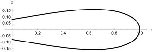
Figure 17: Section of the Heisenberg unit sphere

Figure 18: Sphere $S$ in coordinates $(x,y,z)$

Figure 19: Sphere $S$ in coordinates $(a,b,c)$

Consider the following domains bounded by ellipses in the plane $\mathbb{R}^{2}_{r,z}$:

$$e_{1}\ :\ r^{2}+16\pi^{2}z^{2}\leq 1,$$ (8.3)

$$e_{2}\ :\ r^{2}+12z^{2}\leq 1.$$ (8.4)

Lemma 8.1

The ellipse $\partial e_{1}$ passes through the points $(r,z)=(1,0)$ and $(r,z)=\left(0,\pm\frac{1}{4\pi}\right)$. The intersection $e_{1}\cap\{r\geq 0\}$ is contained inside the curve $(\ref{S1par})$, see Fig. 21. Moreover, the curves $\partial e_{1}\cap\{r\geq 0\}$ and $(\ref{S1par})$ intersect only at the points $(r,z)=(0,\pm\frac{1}{4\pi})$ and $(r,z)=(1,0)$.

Proof.

First of all, it is obvious from $(\ref{S1par})$ and $(\ref{e1})$ that the curves $\partial e_{1}$ and $(\ref{S1par})$ intersect at the points $(r,z)=(0,\pm\frac{1}{4\pi})$ and $(r,z)=(1,0)$.

Further, the ellipse $\partial e_{1}$ is the zero level curve of the function $f_{1}(r,z)=r^{2}+16\pi^{2}z^{2}-1$. Evaluation of this function on the curve $(\ref{S1par})$ is the function $\varphi_{1}(p)=\frac{\sin^{2}p}{p^{2}}+\frac{\pi^{2}}{4p^{4}}(2p-\sin 2p)^{2}-1$. A standard calculus shows that $\varphi_{1}(0)=\varphi_{1}(\pm\pi)=0$, and $\varphi_{1}(p)>0$ for $0<|p|<\pi$, see Fig. 23.

Indeed, we have $\varphi_{1}(p)=f_{1}(p)+f_{2}(p)-1$, $f_{1}(p)=\frac{\sin^{2}p}{p^{2}}$, $f_{2}(p)=\frac{\pi^{2}}{4p^{4}}(2p-\sin 2p)^{2}$. Notice that $f_{2}^{\prime}(p)=\frac{2\pi^{2}}{p^{5}}\cos p(p\cos p-\sin p)(\sin 2p-2p)$.

If $p\in(\pi/2,\pi)$, then $f_{2}^{\prime}(p)<0$, thus $f_{2}(p)$ decreases. Since $f_{2}(\pi)=1$, then $f_{2}(p)>1$, thus $\varphi_{1}(p)>0$ for $p\in(\pi/2,\pi)$.

If $p\in(0,\pi/2)$, then $f_{2}^{\prime}(p)>0$, thus $f_{2}(p)$ increases. Since $f_{2}(\pi/6)=\frac{324}{\pi^{2}}\left(\frac{\pi}{3}-\frac{\sqrt{3}}{2}\right)^{2}\approx 1.08>1$, then $f_{2}(p)>1$ and $\varphi_{1}(p)>0$ for $p\in[\pi/6,\pi/2]$.

In the proof below and in next lemmas we prove bounds of the form $g_{1}(p)<0$, $g_{1}(0)=0$, by comparing $g_{1}(p)$ with appropriate and more simple function $g_{2}(p)$, such that $(g_{1}(p)/g_{2}(p))^{\prime}g_{2}^{2}(p)>0$. We described this method and called it “divide et impera” in [13].

We have the following equalities:

$$\varphi_{1}^{\prime}(p)=\frac{p\cos p-\sin p}{p^{5}}f_{3}(p),$$

$$f_{3}(p)=2(p^{2}+\pi^{2}+\pi^{2}\cos 2p)\sin p-4p\pi^{2}\cos p,$$

$$f_{4}(p)=\left(\frac{f_{3}(p)}{\sin p}\right)^{\prime}\sin^{2}p=2p(1+2\pi^{2}-\cos 2p)+\pi^{2}(\sin 4p-4\sin 2p),$$

$$\left(\frac{f_{4}(p)}{\cos 2p-2\pi^{2}-1}\right)^{\prime}(\cos 2p-2\pi^{2}-1)^{2}=4f_{5}(p)\sin^{2}p,$$

$$f_{5}(p)=-1-7\pi^{2}+(1+2\pi^{2}+8\pi^{4})\cos 2p-\pi^{2}\cos 4p,$$

$$f_{5}^{\prime}(p)=4\cos p\sin pf_{6}(p),$$

$$f_{6}(p)=-1-2\pi^{2}-8\pi^{4}+4\pi^{2}\cos 2p.$$

One has $f_{6}(p)\leq-1+2\pi^{2}-8\pi^{4}<0$ for all $p$, since $\cos 2p\leq 1$. Therefore the restriction to the semi-interval $(0,\pi/6]$ of the function $f_{5}(p)$ decreases, and hence, achieves its minimum at $p=\pi/6$. Its value there is equal to

$$-1-7\pi^{2}+(1+2\pi^{2}+8\pi^{4})/2+\pi^{2}/2=-1/2-5.5\pi^{2}+4\pi^{4}>0.$$

Therefore, $f_{5}(p)>0$ on the above semi-interval. Hence, the function

$$\widetilde{f}_{4}(p):=\frac{f_{4}(p)}{\cos 2p-2\pi^{2}-1}$$

increases there and thus, achieves there its minimum at $p=0$. But $\widetilde{f}_{4}(0)=f_{4}(0)=0$. Therefore, $\widetilde{f}_{4}(p)>0$, hence $f_{4}(p)<0$ for $p\in(0,\pi/6]$. Thus, the function

$$\widetilde{f}_{3}(p):=\frac{f_{3}(p)}{\sin p}$$

decreases on the same semi-interval. Hence, it achieves its supremum there at $p=0$. But $\widetilde{f}_{3}(0)=0$. Therefore, $\widetilde{f}_{3}(p)<0$, hence $f_{3}(p)<0$ on the semi-interval $(0,\pi/6]$. Thus, $\varphi_{1}$ increases there, by the above formula for its derivative and since $p\cos p-\sin p<0$, i.e., $p<\tan p$, whenever $p\in(0,\pi/2)$. But $\varphi_{1}(0)=0$. Hence, $\varphi_{1}>0$ there.

Summing up, if $p\in(0,\pi)$ then $\varphi_{1}(p)>0$. Since $\varphi_{1}(p)$ is even, this inequality holds for $0<|p|<\pi$. ∎

Figure 20: Ellipse $\partial e_{1}$ inside of section of sphere $S$

Figure 21: Ellipse $\partial e_{2}$ outside of section of sphere $S$

Figure 22: Plot of $\varphi_{1}(p)$

Figure 23: Plot of $\varphi_{2}(p)$

Remark 8.2

The ellipse $\partial e_{1}$ is the only ellipse in the plane $(r,z)$, symmetric with respect to the $z$-axis, with the properties given in Lemma 8.1.

Lemma 8.3

The curve $\partial e_{2}$ is tangent to the curve $(\ref{S1par})$ with contact of order $4$. The intersection $\partial e_{2}\cap\{r\geq 0\}$ is contained outside of the curve $(\ref{S1par})$, see Fig. 21. Moreover, the curves $\partial e_{2}\cap\{r\geq 0\}$ and $(\ref{S1par})$ intersect only at the point $(r,z)=(1,0)$.

Proof.

The first statement is obtained by explicit differentiation. Indeed, for the ellipse $\partial e_{2}$ we have $r=\sqrt{1-12z^{2}}=1-6z^{2}+O(z^{4})$, $z\to 0$. And for the curve $(\ref{S1par})$ we have $r(0)=1$, $z(0)=0$. In a neighbourhood of the point $(r,z)=(1,0)$, the curves in question are graphs of even functions $r(z)$. Thus, it is sufficient to prove coincidence of their second derivatives at $z=0$. One has

$$\frac{dr}{dz}=\frac{dr/dp}{dz/dp}=-\frac{2p}{\cos p},$$

$$\frac{d^{2}r}{dz^{2}}=\frac{\frac{d}{dp}(-\frac{2p}{\cos p})}{dz/dp}=\frac{4p^{3}(1+p\tan p)}{\cos^{3}p(p-\tan p)}\to-12,\quad p\to 0,$$

thus $r=1-6z^{2}+O(z^{4})$, $z\to 0$.

The second statement follows since the function $r^{2}+12z^{2}-1$ whose zero level curve is the ellipse $\partial e_{2}$, when restricted to the curve $(\ref{S1par})$, gives the function $\varphi_{2}(p)=\frac{\sin^{2}p}{p^{2}}+\frac{3(2p-\sin 2p)^{2}}{16p^{4}}-1$. A standard calculus shows that $\varphi_{2}(p)<0$ for $0<|p|\leq\pi$, see Fig. 23.

Indeed, we have $\varphi_{2}(p)=f_{1}(p)+f_{2}(p)-1$, $f_{1}(p)=\frac{\sin^{2}p}{p^{2}}$, $f_{2}(p)=\frac{3(2p-\sin 2p)^{2}}{16p^{4}}$. Further,

$$f_{3}(p)=(16p^{4}\varphi_{2}(p))^{\prime}=40p-64p^{3}-40p\cos 2p+4(4p^{2}-3)\sin 2p+6\sin 4p,$$

$$f_{4}(p)=f_{3}^{\prime}(p)=8(5-24p^{2}+4(p^{2}-2)\cos 2p+3\cos 4p+14p\sin 2p),$$

$$f_{5}(p)=f_{4}^{\prime}(p)=-16(-18p\cos 2p+(4p^{2}-15)\sin 2p+6(4p+\sin 4p)),$$

$$f_{6}(p)=f_{5}^{\prime}(p)=-64(6+2(p^{2}-6)\cos 2p+6\cos 4p+11p\sin 2p),$$

$$f_{7}(p)=\left(\frac{f_{6}(p)}{\cos 2p}\right)^{\prime}\cos^{2}2p=32(-48p-4p\cos 4p+12\sin 2p-11\sin 4p+12\sin 6p),$$

$$f_{8}(p)=f_{7}^{\prime}(p)=512f_{9}(p)f_{10}(p),$$

$$f_{9}(p)=\sin p-\sin 3p,\qquad f_{10}(p)=-2p\cos p+3\sin p+9\sin 3p,$$

$$f_{11}(p)=\left(\frac{f_{10}(p)}{\cos p}\right)^{\prime}\cos^{2}p=2+17\cos 2p+9\cos 4p.$$

Let $p\in(0,\frac{\pi}{8}]$, then $f_{11}(p)>0$, thus $\tilde{f}_{10}(p)=\frac{f_{10}(p)}{\cos p}$ increases. Since $\tilde{f}_{10}(0)=0$, then $\tilde{f}_{10}(p)>0$, so $f_{10}(p)>0$.

Let $p\in(\frac{\pi}{8},\frac{\pi}{4})$. Then $-2p\cos p>-\frac{\pi}{2}\cos\frac{\pi}{4}\approx-1.11>-2$, $3\sin p>3\sin\frac{\pi}{8}\approx 1.14>1$, $9\sin 3p>9\sin\frac{3\pi}{4}\approx 6.36>6$, thus $f_{10}(p)>-2+1+6>0$.

Now let $p\in(0,\pi/4)$, we have proved that $f_{10}(p)>0$. Since $f_{9}(p)<0$, then $f_{8}(p)<0$, thus $f_{7}(p)$ decreases. Since $f_{7}(0)=0$, then $f_{7}(p)<0$, thus $\tilde{f}_{6}(p)=\frac{f_{6}(p)}{\cos 2p}$ decreases. Since $\tilde{f}_{6}(0)=0$ then $\tilde{f}_{6}(p)<0$, thus $f_{6}(p)<0$. Thus $f_{5}(p)$ decreases, and since $f_{5}(0)=0$ then $f_{5}(p)<0$. Thus $f_{4}(p)$ decreases, and since $f_{4}(0)=0$ then $f_{4}(p)<0$. Thus $f_{3}(p)$ decreases, and since $f_{3}(0)=0$ then $f_{3}(p)<0$. Thus $p^{4}\varphi_{2}(p)$ decreases, and since $\lim_{p\to 0}p^{4}\varphi_{2}(p)=0$ then $\varphi_{2}(p)<0$ for $p\in(0,\pi/4]$.

If $p\in(\pi/4,3\pi/8)$, then $-48p<-12\pi<-37.6$, $|4p\cos 4p|<3\pi/2<4.72$, $|12\sin 6p|<12$. One has $|12\sin 2p-11\sin 4p|<20.3$, since this is true at the endpoints $p=\pi/4,3\pi/8$ and at the extremum point of the function under modulus in the interval in question. Indeed, its derivative in $x=2p\in(\pi/2,3\pi/4)$ is equal to $12\cos x-22\cos 2x=12u-22(2u^{2}-1)$, $u=\cos x$. The latter derivative vanishes, if and only if $22u^{2}-6u-11=0$. Solving the latter quadratic equation in negative $u=\cos x$ (which is indeed negative in the given interval) yields

$$u=\cos x=\frac{3-\sqrt{251}}{22}\approx-0.58377,\ \sin x=\sqrt{1-u^{2}}\approx\sqrt{0.65921}\approx 0.811,$$

$$|12\sin 2p-11\sin 4p|=2\sin x(6-11\cos x)\approx 20.169<20.3.$$

Thus, $\frac{f_{7}(p)}{32}<-37.6+4.72+20.3+12<0$. If $p\in[3\pi/8,\pi/2)$, then $-48p<-50$, $-4p\cos 4p\leq 0$, $|12\sin 2p-11\sin 4p+12\sin 6p|<35$, thus $\frac{f_{7}(p)}{32}<-50+35<0$.

Thus for $p\in(\pi/4,\pi/2)$ we have $f_{7}(p)<0$, so repeating the argument used two paragraphs above we get $f_{i}(p)<0$ for $i=3,\dots,6$, hence $\varphi_{2}(p)<0$.

Finally, if $p\in[\pi/2,\pi)$, then $f_{1}(p)\leq\frac{4}{\pi^{2}}<\frac{1}{2}$. Since

$$f_{2}^{\prime}(p)=-\frac{3}{p^{5}}\cos p(p\cos p-\sin p)(p-\cos p\sin p)\leq 0,$$

then $f_{2}(p)$ decreases, and since $f_{2}(\frac{\pi}{2})=\frac{3}{\pi^{2}}\approx 0.3$ then $f_{2}(p)<\frac{1}{2}$. Thus $\varphi_{2}(p)<0$.

If $p=\pi$ then $\varphi_{2}(p)=\frac{3-4\pi^{2}}{4\pi^{2}}<0$.

We proved that $\varphi_{2}(p)<0$ for $p\in(0,\pi]$. Since $\varphi_{2}(p)$ is even, this inequality holds for $0<|p|\leq\pi$. ∎

Remark 8.4

The ellipse $\partial e_{2}$ is the smallest ellipse in the plane $(r,z)$ among ellipses symmetric with respect to the $z$-axis, tangent to the curve $(\ref{S1par})$ at the point $(r,z)=(1,0)$ and encircling this curve.

Consider the projection

$$P\,:\,\mathbb{R}^{3}_{x,y,z}\to\{(r,z)\in\mathbb{R}^{2}\mid r\geq 0\},$$

$$P(x,y,z)=(r,z)=(\sqrt{x^{2}+y^{2}},z)$$

and the corresponding ellipsoids $E_{i}=P^{-1}(e_{i})$, $i=1,2$. Lemmas 8.1 and 8.3 plus equality $(\ref{dilat})$ imply obviously the following two-sided ellipsoidal bounds of sub-Riemannian balls

$$B_{R}:=\{g\in G\mid d(\operatorname{Id},g)\leq R\}$$

on the Heisenberg group.

Corollary 8.5

For any $R>0$ we have

$$\delta_{R}(E_{1})\subset B_{R}\subset\delta_{R}(E_{2}).$$ (8.5)

Remark 8.6

Estimates $(\ref{ball_bounds})$ are sharp in the sense that the ellipsoids $\delta_{R}(E_{1})$ and $\delta_{R}(E_{2})$ are tangent to the sub-Riemannian ball $B_{R}$ at its points in the plane $\{z=0\}$. Moreover, the ellipsoid $\delta_{R}(E_{1})$ intersects the sub-Riemannian ball $B_{R}$ at its points in the line $\{x=y=0\}$, see Figs. 21, 21.

Remark 8.7

In order to estimate precision of bounds $(\ref{ball_bounds})$, take the Euclidean volume $V=dx\wedge dy\wedge dz$ (in fact, Popp’s volume [2]). Then

$$V(E_{1})=\frac{1}{4}<V(B_{1})=\frac{1}{12}\left(1+2\pi\int_{0}^{2\pi}\frac{\sin x}{x}dx\right)\approx 0.83\\ <V(E_{2})=\frac{\pi}{2\sqrt{3}}\approx 0.91.$$

The above integral formula for the volume $V(B_{1})$ was proved in [14], P. 587.

Corollary 8.8

Let $g=(x,y,z)\in G$, and let $r=\sqrt{x^{2}+y^{2}}$. Then

$$\underline{d}(g):=\sqrt{\frac{\sqrt{r^{4}+48z^{2}}+r^{2}}{2}}\leq d(\operatorname{Id},g)\leq\sqrt{\frac{\sqrt{r^{4}+64\pi^{2}z^{2}}+r^{2}}{2}}=:\overline{d}(g).$$ (8.6)

Proof.

Since the statement holds trivially for $g=\operatorname{Id}=(0,0,0)$, we can assume that $g\neq\operatorname{Id}$, then $R:=d(\operatorname{Id},g)>0$. Denote $g^{\prime}=\delta_{\frac{1}{R}}(g)$, then $d(\operatorname{Id},g^{\prime})=1$, and inclusions $(\ref{ball_bounds})$ imply that the functions $f_{1}(x,y,z)=r^{2}+16\pi^{2}z^{2}$ and $f_{2}(x,y,z)=r^{2}+12z^{2}$, $r=\sqrt{x^{2}+y^{2}}$, satisfy the inequalities

$$f_{1}(g^{\prime})=f_{1}\left(\frac{x}{R},\frac{y}{R},\frac{z}{R^{2}}\right)\geq 1=d(\operatorname{Id},g^{\prime})\geq f_{2}\left(\frac{x}{R},\frac{y}{R},\frac{z}{R^{2}}\right)=f_{2}(g^{\prime}).$$

Thus $\frac{r^{2}}{R^{2}}+16\pi^{2}\frac{z^{2}}{R^{4}}\geq 1\geq\frac{r^{2}}{R^{2}}+12\frac{z^{2}}{R^{4}}$, i.e.,

$$16\pi^{2}z^{2}\alpha^{2}+r^{2}\alpha\geq 1\geq 12z^{2}\alpha^{2}+r^{2}\alpha,\qquad\alpha=\frac{1}{R^{2}}.$$ (8.7)

The second inequality in $(\ref{al})$ solves to $0<\alpha\leq\alpha_{2}:=\frac{2}{\sqrt{r^{4}+48z^{2}}+r^{2}}$, whence $R\geq\frac{1}{\sqrt{\alpha_{2}}}=\sqrt{\frac{\sqrt{r^{4}+48z^{2}}+r^{2}}{2}}$, which gives the first inequality in $(\ref{dleq})$. Similarly, the first inequality in $(\ref{al})$ solves to $\alpha\geq\alpha_{1}:=\frac{2}{\sqrt{r^{4}+64\pi^{2}z^{2}}+r^{2}}$, whence $R\leq\frac{1}{\sqrt{\alpha_{1}}}=\sqrt{\frac{\sqrt{r^{4}+64\pi^{2}z^{2}}+r^{2}}{2}}$, which gives the second inequality in $(\ref{dleq})$. ∎

Remark 8.9

Estimates $(\ref{dleq})$ are functional expressions of bounds $(\ref{ball_bounds})$:

$$\{g\in G\mid\underline{d}(g)\leq R\}=\delta_{R}(E_{2}),\qquad\{g\in G\mid\overline{d}(g)\leq R\}=\delta_{R}(E_{1}).$$

Remark 8.10

Estimates $(\ref{dleq})$ are sharp in the following sense:

1. in the case $z=0$ these inequalities turn into equalities,

2. in the case $r=0$ the second inequality turns into equality corresponding to $e_{1}$.

In the case $rz\neq 0$ the both inequalities $(\ref{dleq})$ are strict.

The second inclusion in $(\ref{ball_bounds})$ obviously implies the following inclusions.

Corollary 8.11

For any $R>0$ we have

$$B_{R}\subset\left\{g=(x,y,z)\in G\mid\sqrt{x^{2}+y^{2}}\leq R\right\},$$

$$B_{R}\subset\left\{g=(x,y,z)\in G\mid|z|\leq\frac{R^{2}}{\sqrt{12}}\right\},$$

or, which is equivalent,

$$d(\operatorname{Id},g)\geq\sqrt{x^{2}+y^{2}},$$ (8.8)

$$d(\operatorname{Id},g)\geq\sqrt[4]{12z^{2}}.$$ (8.9)

Notice that inequalities $(\ref{d>=1})$, $(\ref{d>=2})$ follow also from the first inequality in $(\ref{dleq})$.

9 Bounds of cut time via lower bounds
of sub-Riemannian balls

Fix a point $q_{0}=g_{0}^{\prime}\in M$. Denote the ball $B^{\prime}_{t}=\{q\in M\mid d^{\prime}(q_{0},q)\leq t\}$, $t\geq 0$, where $d^{\prime}$ is the sub-Riemannian distance on $M$. Denote also

$$\bar{t}=\inf\{t>0\mid B^{\prime}_{t}=M\}.$$

The following lemmas show the relevance of the number $\bar{t}$ for the sub-Riemannian manifold $M$.

Lemma 9.1

We have the following:

• $\bar{t}=\sup\{d^{\prime}(q_{0},q_{1})\mid q_{1}\in M\}$.

• $\bar{t}=\sup\{t_{\operatorname{cut}}(q(\cdot))\mid q(\cdot)\subset M\text{ a geodesic s.t. }q(0)=q_{0}\}$.

Proof.

(1) Denote $t_{1}=\sup\{d^{\prime}(q_{0},q_{1})\mid q_{1}\in M\}$ and assume by contradiction that $\bar{t}\neq t_{1}$.

Let $t_{1}<\bar{t}$. Then for every $t\in(t_{1},\bar{t})$ and every $q_{1}\in M$ we have $d^{\prime}(q_{0},q_{1})<t$, i.e., $q_{1}\in B^{\prime}_{t}$. Since $t<\bar{t}$, this contradicts to definition of $\bar{t}$.

Let $t_{1}>\bar{t}$. Then for every $t\in(\bar{t},t_{1})$ there exists $q_{1}\in M$ such that $d^{\prime}(q_{0},q_{1})>t$, i.e., $q_{1}\notin B^{\prime}_{t}$. Since $t>\bar{t}$, this contradicts to definition of $\bar{t}$ once more.

(2) Denote $t_{2}=\sup\{t_{\operatorname{cut}}(q(\cdot))\mid q(\cdot)\subset M\text{ a geodesic s.t. }q(0)=q_{0}\}$ and assume by contradiction that $\bar{t}\neq t_{2}$.

Let $t_{2}<\bar{t}$, take any $t\in(t_{2},\bar{t})$. Then $B^{\prime}_{t}\neq M$, thus there exists a point $q_{1}\in M$ such that $d^{\prime}(q_{0},q_{1})>t$. Take a sub-Riemannian length minimizer $q(\cdot)$ connecting $q_{0}$ and $q_{1}$. We have $t_{\operatorname{cut}}(q(\cdot))>t>t_{2}$, which contradicts the definition of $t_{2}$.

Let $\bar{t}<t_{2}$, take any $t\in(\bar{t},t_{2})$. We have $B^{\prime}_{t}=M$, thus for every $q_{1}\in M$ one has the inequality $d^{\prime}(q_{0},q_{1})\leq t$. Then for every geodesic $q(\cdot)\subset M$ starting at $q_{0}$ we have $t_{\operatorname{cut}}(q(\cdot))\leq t<t_{2}$, which contradicts the definition of $t_{2}$. ∎

Remark 9.2

Consider the diameter of the sub-Riemannian manifold $M$:

$$\operatorname{diam}(M)=\sup\{d^{\prime}(q_{1},q_{2})\mid q_{1},q_{2}\in M\}.$$

By the triangle inequality, we have a bound $\operatorname{diam}(M)\leq 2\bar{t}$.

Theorem 9.3

We have $\bar{t}\leq t_{*}:=\frac{1}{2}\sqrt{\frac{1}{2}\left(1+\sqrt{1+1024\pi^{2}}\right)}\approx 3.56$.

Proof.

We show that $B^{\prime}_{t_{*}}=M$. By Corollary 8.5, we have $B_{t_{*}}\supset\delta_{t_{*}}(E_{1})=:E_{1t_{*}}$, where the ellipsoid $E_{1t_{*}}\subset G$ is defined by the inequality $\frac{r^{2}}{{t_{*}^{2}}}+\frac{16\pi^{2}z^{2}}{{t_{*}^{4}}}\leq 1$. Thus $B^{\prime}_{t_{*}}\supset E^{\prime}_{1{t_{*}}}:=\pi(E_{1{t_{*}}})$. We show that $E^{\prime}_{1{t_{*}}}=M$.

The homogeneous space $M$ can be represented by a fundamental domain $D=\{(a,b,c)\in G\mid 0\leq a,b,c<1\}$, so that $\pi(D)=M$. We have $D\subset\cup_{i=1}^{8}K_{i}$, where the cubes $K_{i}$ are defined as follows:

$$K_{1}\ :\ 0\leq a,b,c\leq\frac{1}{2},\qquad K_{2}\ :\ 0\leq a,c\leq\frac{1}{2}\leq b\leq 1,$$

$$K_{3}\ :\ 0\leq a\leq\frac{1}{2}\leq b,c\leq 1,\qquad K_{4}\ :\ 0\leq a,b\leq\frac{1}{2}\leq c\leq 1,$$

$$K_{5}\ :\ 0\leq b,c\leq\frac{1}{2}\leq a\leq 1,\qquad K_{6}\ :\ 0\leq c\leq\frac{1}{2}\leq a,b\leq 1,$$

$$K_{7}\ :\ \frac{1}{2}\leq a,b,c\leq 1,\qquad K_{8}\ :\ 0\leq b\leq\frac{1}{2}\leq a,c\leq 1.$$

We show that $E^{\prime}_{1{t_{*}}}\supset\pi(K_{i})$, $i=1,\dots,8$, which implies that $E^{\prime}_{1{t_{*}}}=M$. To this end we define the following points $g_{i}\in H$ in the coordinates $(a,b,c)$: $g_{1}=(0,0,0)$, $g_{2}=(0,1,0)$, $g_{3}=(0,1,1)$, $g_{4}=(0,0,1)$, $g_{5}=(1,0,0)$, $g_{6}=(1,1,0)$, $g_{7}=(1,1,1)$, $g_{8}=(1,0,1)$, and prove that $E_{1t_{*}}\supset\tilde{K}_{i}:=g_{i}^{-1}K_{i}$, $i=1,\dots,8$.

Let $L\subset\mathbb{R}^{n}$ be a convex compact set. We call a continuous function $f\,:\,L\to\mathbb{R}$ quasiconvex if $\max_{L}f=\max_{\partial L}f$. Since a convex function on a convex compact set attains maximum at points of the boundary of this set or at all points of this set, then a convex function on such a set is quasiconvex.

Now let $\Pi\subset\mathbb{R}^{3}$ be a parallelepiped whose all faces and edges are parallel to coordinate planes and axes, and let $\dim\Pi\in\{1,2,3\}$, i.e., $\Pi$ is a 3D parallelepiped, a 2D rectangle, or a 1D segment. Let us study quasiconvexity of the function $f_{t}(a,b,c)=t^{2}(a^{2}+b^{2})+4\pi^{2}(2c-ab)^{2}-t^{4}$ whose zero level is the ellipsoid $\partial E_{1t}$, $t>0$. We have $\frac{\partial\,f_{t}}{\partial\,a}=2t^{2}a-8\pi^{2}b(2c-ab)$, $\frac{\partial\,f_{t}}{\partial\,b}=2t^{2}b-8\pi^{2}a(2c-ab)$, $\frac{\partial\,f_{t}}{\partial\,c}=16\pi^{2}(2c-ab)$, thus $f_{t}$ has only one critical point $(a,b,c)=(0,0,0)$, which is the minimum point. Thus if $\dim\Pi=3$ then $\left.f_{t}\right|_{\Pi}$ is quasiconvex.

If $\Pi\subset\{a=\operatorname{const}\}$ or $\Pi\subset\{b=\operatorname{const}\}$, then $\left.f_{t}\right|_{\Pi}$ is convex, thus it is quasiconvex. Thus if $\dim\Pi=3$ and the restriction of $f_{t}$ to faces of $\Pi$ parallel to the plane $\{c=0\}$ is quasiconvex, then $\left.f_{t}\right|_{\Pi}$ attains maximum at vertices of $\Pi$.

1) We prove that $E_{1t_{*}}\supset\tilde{K}_{1}=K_{1}$. Since $\left.\frac{\partial\,f_{t}}{\partial\,a}\right|_{c=0}={2a(4\pi^{2}b^{2}+t^{2})}$, which is nonnegative and vanishes only for $a=0$, then the function
$\left.f_{t_{*}}\right|_{K_{1}\cap\{c=0\}}$ increases in $a$, thus $\left.f_{t}\right|_{K_{1}\cap\{c=0\}}$ is quasiconvex.

We have $p:=\left(\left.\frac{\partial\,f_{t_{*}}}{\partial\,a}+\frac{\partial\,f_{t_{*}}}{\partial\,b}\right)\right|_{K_{1}\cap\{c=1/2\}}=2(a+b)(t_{*}^{2}-4(1-ab)\pi^{2})$. Since in $K_{1}$ we have $ab\leq\frac{1}{4}<1-\frac{t_{*}^{2}}{4\pi^{2}}\approx 0.68$, then $p$ is nonpositive and vanishes only at $(a,b)=(0,0)$, then $\left.f_{t_{*}}\right|_{K_{1}\cap\{c=1/2\}}$ is quasiconvex.

Thus $\left.f_{t_{*}}\right|_{K_{1}}$ attains maximum at vertices of $K_{1}$. We have $f_{t_{*}}(0,0,0)\approx-161$, $f_{t_{*}}(0,0,1/2)\approx-122$, $f_{t_{*}}(0,1/2,0)=f_{t_{*}}(1/2,0,0)\approx-158$,
$f_{t_{*}}(0,1/2,1/2)=f_{t_{*}}(1/2,0,1/2)\approx-118$, $f_{t_{*}}(1/2,1/2,0)\approx-152$,
$f_{t_{*}}(1/2,1/2,1/2)\approx-133$, whence $\left.f_{t_{*}}\right|_{K_{1}}<0$, thus $E_{1t_{*}}\supset\tilde{K}_{1}=K_{1}$.

2) We prove that $E_{1t_{*}}\supset\tilde{K}_{2}=g_{2}^{-1}K_{2}$. Notice that for any elements $(\alpha,\beta,\gamma)$, $(a,b,c)$ of $G$

$$(\alpha,\beta,\gamma)^{-1}\cdot(a,b,c)=(a-\alpha,b-\beta,c-\gamma+\alpha(\beta-b)).$$

Thus $\tilde{K}_{2}=\{a,c\in[0,1/2],\ b\in[-1/2,0]\}$. By the argument of item 1), the function $\left.f_{t_{*}}\right|_{\tilde{K}_{2}\cap\{c=0\}}$ increases in $a$, thus $\left.f_{t}\right|_{\tilde{K}_{2}\cap\{c=0\}}$ is quasiconvex.

We have $\left.\frac{\partial\,f_{t}}{\partial\,a}\right|_{\tilde{K}_{2}\cap\{c=1/2\}}=8b(ab-1)\pi^{2}+2at^{2}$, which is nonnegative and vanishes only for $a=b=0$, thus $\left.f_{t}\right|_{\tilde{K}_{2}\cap\{c=1/2\}}$ is quasiconvex.

So $\left.f_{t_{*}}\right|_{\tilde{K}_{2}}$ attains maximum at vertices of $\tilde{K}_{2}$. In item 1) we showed that $f_{t_{*}}<0$ at vertices of the square $[0,1/2]_{a}\times\{b=0\}\times[0,1/2]_{c}$. Further, we have $f_{t_{*}}(0,-1/2,0)\approx-158$, $f_{t_{*}}(0,-1/2,1/2)\approx-118$, $f_{t_{*}}(1/2,-1/2,0)\approx-152$, $f_{t_{*}}(1/2,-1/2,1/2)\approx-93$, then $\left.f_{t_{*}}\right|_{\tilde{K}_{2}}<0$, thus $E_{1t_{*}}\supset\tilde{K}_{2}$.

3) We prove that $E_{1t_{*}}\supset\tilde{K}_{3}=g_{3}^{-1}K_{3}=\{a\in[0,1/2],\ b,c\in[-1/2,0]\}$. Consider the involution $i\,:\,(a,b,c)\mapsto(a,-b,-c)$. Then $i(\tilde{K}_{1})=\tilde{K}_{3}$ and $f_{t}\circ i=f_{t}$, thus $\left.f_{t_{*}}\right|_{\tilde{K}_{3}}<0$ since $\left.f_{t_{*}}\circ i\right|_{\tilde{K}_{1}}=\left.f_{t_{*}}\right|_{\tilde{K}_{1}}<0$. Thus $E_{1t_{*}}\supset\tilde{K}_{3}$.

4) We prove that $E_{1t_{*}}\supset\tilde{K}_{4}=g_{4}^{-1}K_{4}=\{a,b\in[0,1/2],\ c\in[-1/2,0]\}$. Consider the involution $i\,:\,(a,b,c)\mapsto(a,-b,-c)$. Then $i(\tilde{K}_{2})=\tilde{K}_{4}$ and $f_{t}\circ i=f_{t}$, thus $\left.f_{t_{*}}\right|_{\tilde{K}_{4}}<0$ by virtue of $\left.f_{t_{*}}\right|_{\tilde{K}_{2}}<0$ similarly to item 3).

5) We prove that $E_{1t_{*}}\supset\tilde{K}_{5}=g_{5}^{-1}K_{5}$. We have $\tilde{K}_{5}\subset\hat{K}_{5}=\{a\in[-1/2,0],\ b\in[0,1/2],\ c\in[-1/2,1/2]\}$. Notice that $\left.\frac{\partial\,f_{t}}{\partial\,a}\right|_{c=-1/2}=2a(t^{2}+4\pi^{2}b^{2})+8\pi^{2}b=0$ only if $a=\bar{a}:=-\frac{4\pi^{2}b}{t^{2}+4\pi^{2}b^{2}}$, and

$$\left.\frac{\partial\,f_{t_{*}}}{\partial\,b}\right|_{a=\bar{a},\ b\in[0,1/2],\ c=-1/2}=\frac{2bt_{*}^{2}(16\pi^{4}(b^{4}-1)+8b^{2}\pi^{2}t_{*}^{2}+t_{*}^{4})}{(4b^{2}\pi^{2}+t_{*}^{2})^{2}},$$

which is nonpositive (since the quartic polynomial in brackets in numerator is negative for $b\in[0,1/2]$) and vanishes only for $b=0$. Thus $\left.f_{t_{*}}\right|_{\hat{K}^{5}\cap\{c=-1/2\}}$ has no interior critical points, so this function is quasiconvex.

We have $\left.\frac{\partial\,f_{t}}{\partial\,a}\right|_{\hat{K}^{5}\cap\{c=1/2\}}=2a(t^{2}+4\pi^{2}b^{2})-8\pi^{2}b=0$ only if $a=\bar{a}:=\frac{4\pi^{2}b}{t^{2}+4\pi^{2}b^{2}}$, and $\left.\frac{\partial\,f_{t_{*}}}{\partial\,b}\right|_{a=\bar{a},\ b\in[0,1/2],\ c=1/2}=\frac{2bt_{*}^{2}(16\pi^{4}(b^{4}-1)+8b^{2}\pi^{2}t_{*}^{2}+t_{*}^{4})}{(4b^{2}\pi^{2}+t_{*}^{2})^{2}}$, which is nonpositive and vanishes only for $b=0$ by the previous paragraph. Thus $\left.f_{t_{*}}\right|_{\hat{K}_{5}\cap\{c=1/2\}}$ has no interior critical points, so this function is quasiconvex.

So $\left.f_{t_{*}}\right|_{\hat{K}_{5}}$ attains maximum at vertices of $\hat{K}_{5}$. Since $f_{t_{*}}(-1/2,0,-1/2)=f_{t_{*}}(-1/2,0,1/2)=f_{t_{*}}(1/2,0,1/2)=f_{t_{*}}(0,1/2,1/2)=f_{t_{*}}(0,1/2,-1/2)\approx-118$, $f_{t_{*}}(-1/2,1/2,-1/2)=f_{t_{*}}(1/2,1/2,1/2)\approx-132$, $f_{t_{*}}(-1/2,1/2,1/2)=f_{t_{*}}(1/2,-1/2,1/2)\approx-93$, $f_{t_{*}}(0,0,-1/2)=f_{t_{*}}(0,0,1/2)\approx-121$, see items 1)–3) above, then $\left.f_{t_{*}}\right|_{\hat{K}_{5}}\leq 0$, thus $\left.f_{t_{*}}\right|_{\tilde{K}_{5}}\leq 0$, and $E_{1t_{*}}\supset\tilde{K}_{5}$.

6) We prove that $E_{1t_{*}}\supset\tilde{K}_{6}=g_{6}^{-1}K_{6}$. We have $\tilde{K}_{6}\subset\hat{K}_{6}=\{a,b\in[-1/2,0],\ c\in[0,1]\}$. Since $\left.\frac{\partial\,f_{t}}{\partial\,a}\right|_{\hat{K}_{6}\cap\{c=0\}}=2a(4b^{2}\pi^{2}+t^{2})$, which is nonpositive and vanishes only for $a=0$, then $\left.f_{t}\right|_{\hat{K}_{6}\cap\{c=0\}}$ is quasiconvex.

We have $\delta:=\left.\left(\frac{\partial\,f_{t}}{\partial\,a}+\frac{\partial\,f_{t}}{\partial\,b}\right)\right|_{\hat{K}_{6}\cap\{c=1\}}=2(a+b)(t^{2}-4\pi^{2}(2-ab))$. Since $\frac{t_{*}^{2}}{4\pi^{2}}\approx 0.32<\frac{7}{4}\leq 2-ab$, then $\delta$ is nonnegative and vanishes only for $a=b=0$. Thus $\left.f_{t}\right|_{\hat{K}_{6}\cap\{c=1\}}$ is quasiconvex. So $\left.f_{t_{*}}\right|_{\tilde{K}_{6}}$ attains maximum at vertices of $\tilde{K}_{6}$.

Since $f_{t_{*}}(-1/2,-1/2,0)=f_{t_{*}}(1/2,1/2,0)\approx-152$, see item 1),
$f_{t_{*}}(-1/2,-1/2,1)\approx-34$,
$f_{t_{*}}(-1/2,0,0)=f_{t_{*}}(0,-1/2,0)\approx-158$, see item 1), $f_{t_{*}}(-1/2,0,1)=f_{t_{*}}(0,-1/2,1)=0$, $f_{t_{*}}(0,0,0)\approx-161$, see item 1), $f_{t_{*}}(0,0,1)\approx-3$, then $\left.f_{t_{*}}\right|_{\hat{K}^{6}}\leq 0$, thus $\left.f_{t_{*}}\right|_{\tilde{K}^{6}}\leq 0$, and $E_{1t_{*}}\supset\tilde{K}_{6}$.

7) We prove that $E_{1t_{*}}\supset\tilde{K}_{7}=g_{7}^{-1}K_{7}$. We have $\tilde{K}_{7}\subset\hat{K}_{7}=\{a,b\in[-1/2,0],\ c\in[-1/2,1/2]\}$. Consider the involution $i\,:\,(a,b,c)\to(a,-b,-c)$. Then $i(\hat{K}_{5})=\hat{K}_{7}$ and $f_{t}\circ i=f_{t}$. Since $\left.f_{t_{*}}\right|_{\tilde{K}^{5}}\leq 0$, then $\left.f_{t_{*}}\right|_{\tilde{K}^{7}}\leq 0$, and $E_{1t_{*}}\supset\tilde{K}_{7}$.

8) Finally, we prove that $E_{1t_{*}}\supset\tilde{K}_{8}=g_{8}^{-1}K_{8}$. We have $\tilde{K}_{8}\subset\hat{K}_{8}=\{a\in[-1/2,0],\ b\in[0,1/2],\ c\in[-1,0]\}$. Consider the involution $i\,:\,(a,b,c)\to(a,-b,-c)$. Then $i(\hat{K}_{6})=\hat{K}_{8}$ and $f_{t}\circ i=f_{t}$. Since $\left.f_{t_{*}}\right|_{\tilde{K}^{6}}\leq 0$, then $\left.f_{t_{*}}\right|_{\tilde{K}^{8}}\leq 0$, and $E_{1t_{*}}\supset\tilde{K}_{8}$.

Summing up, we proved that $E_{1t_{*}}\supset\cup_{i=1}^{8}g_{i}^{-1}K_{i}$. Thus

$$E^{\prime}_{1t_{*}}\supset\cup_{i=1}^{8}\pi(g_{i}^{-1}(K_{i}))\supset\pi(D)=M,$$

so the required inclusion $B^{\prime}_{t_{*}}=M$ follows. ∎

We plot a union of sub-Riemannian balls $B_{t_{*}}(h)$ for some $h\in H$ covering the fundamental domain $D$ in Fig. 24.

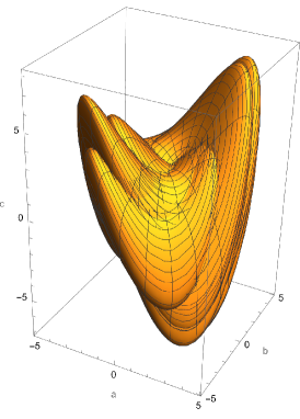
Figure 24: Union of sub-Riemannian Heisenberg balls $B_{t}(h)$ covering the fundamental domain $D$

Now we provide a lower bound of the number $\bar{t}$. Denote the points $\bar{g}=(\bar{a},\bar{b},\bar{c}),\tilde{g}=(\tilde{a},\tilde{b},\tilde{c})\in G$ such that $\bar{a}=\bar{b}=\bar{c}=\frac{1}{2}$ and $\tilde{a}=1$, $\tilde{b}=\tilde{c}=0$.

Theorem 9.4

We have $\bar{t}\geq d(\tilde{g},\bar{g})$.

Proof.

By left-invariance of the metric $d$, for any $g_{1},g_{2}\in G$ we have $d(g_{1},g_{2})=d(\operatorname{Id},g_{0})$, $g_{0}=g_{1}^{-1}g_{2}$. The distance $d(\operatorname{Id},g_{0})$, $g_{0}=(x,y,z)$, is computed explicitly [11]: if $(x,y)\neq(0,0)$ then

$$d(\operatorname{Id},g_{0})=\frac{p}{\sin p}\sqrt{x^{2}+y^{2}},$$ (9.1)

$$\frac{2p-\sin 2p}{8\sin^{2}p}=\frac{|z|}{x^{2}+y^{2}},\qquad p\in[0,\pi],$$ (9.2)

and if $(x,y)=(0,0)$ then $d(\operatorname{Id},g_{0})=2\sqrt{\pi|z|}$.

Now we show that $d(\tilde{g},\bar{g})<1$. We have $d(\tilde{g},\bar{g})=d(\operatorname{Id},g)$, where $g=\tilde{g}^{-1}\bar{g}=(x,y,z)=(-1/2,1/2,1/8)$. The function $\psi(p):=\frac{2p-\sin 2p}{8\sin^{2}p}$ that appears in $(\ref{dist2})$ increases as $p\in(0,\pi)$ from $0$ to $+\infty$. Indeed, changing $p$ to $u=2p$, we get

$$4(1-\cos u)^{2}\frac{d\psi}{du}=(1-\cos u)^{2}-(u-\sin u)\sin u=2(1-\cos u)-u\sin u$$

$$=4\sin p(\sin p-p\cos p)>0\ \text{ for }\ p\in(0,\pi).$$

Since $\psi(1.25)\approx 0.26$ then $\psi(1.25)>\frac{1}{4}$. Let $p_{*}\in(0,\pi)$ be the root of the equation $\psi(p_{*})=\frac{1}{4}=\frac{|z|}{x^{2}+y^{2}}$. Then $p_{*}=\psi^{-1}(\frac{1}{4})<1.25$, thus by equalities $(\ref{dist1})$, $(\ref{dist2})$

$$d(\operatorname{Id},\tilde{g}^{-1}\bar{g})=\frac{p_{*}}{\sin p_{*}}\sqrt{\left(\frac{1}{2}\right)^{2}+\left(\frac{1}{2}\right)^{2}}<\frac{1.25}{\sin 1.25}\frac{1}{\sqrt{2}}\approx 0.93<1.$$

Here we use increasing of the function $\frac{p}{\sin p}$ in $p\in(0,\pi)$. Indeed, its derivative multiplied by $\sin^{2}p$ is equal to $\sin p-p\cos p>0$. So $d(\tilde{g},\bar{g})<1$.

Take any number $\tilde{t}\in(0,d(\tilde{g},\bar{g}))$. We show that $B^{\prime}_{\tilde{t}}\neq M$. To this end we show that $\pi(\bar{g})\notin B^{\prime}_{\tilde{t}}$, i.e., that $\bar{g}\notin HB_{\tilde{t}}$.

We take any $h=(a,b,c)\in H$ and show that $\bar{g}\notin hB_{\tilde{t}}$. The following cases are possible:

1) $0\leq a,b,c\leq 1$,

2) $(a\leq-1)\quad\lor\quad(a\geq 2)\quad\lor\quad(b\leq-1)\quad\lor\quad(b\geq 2)$,

3) $(0\leq a,b\leq 1)\quad\land\quad((c\leq-1)\quad\lor\quad(c\geq 2))$.

1) Let $0\leq a,b,c\leq 1$.

1.1) Let $h=(0,0,0)$ in coordinates $a,b,c$, we denote this as $h=(0,0,0)_{abc}$. Then $g_{0}=h^{-1}\bar{g}=\bar{g}=(1/2,1/2,1/2)_{abc}=(1/2,1/2,3/8)_{xyz}$, i.e., the point $\bar{g}$ has coordinates $(x,y,z)=(1/2,1/2,3/8)$. Thus by Corollary 8.8 $d(\operatorname{Id},g_{0})\geq\underline{d}(g_{0})=\sqrt{\frac{1}{2}\left(\frac{1}{2}+\sqrt{7}\right)}\approx 1.25>1>d(\tilde{g},\bar{g})>\tilde{t}$.

1.2) Let $h=(0,0,1)_{abc}$. Then $g_{0}=h^{-1}\bar{g}=(1/2,1/2,-1/2)_{abc}=(1/2,1/2,-5/8)_{xyz}$, thus by Corollary 8.8
$d(\operatorname{Id},g_{0})\geq\underline{d}(g_{0})=\sqrt{\frac{1}{2}\left(\frac{1}{2}+\sqrt{19}\right)}\approx 1.56>1>d(\tilde{g},\bar{g})>\tilde{t}$.

1.3) Let $h=(0,1,0)_{abc}$.
Then $g_{0}=h^{-1}\bar{g}=(1/2,-1/2,1/2)_{abc}=(1/2,-1/2,5/8)_{xyz}$, thus by Corollary 8.8
$d(\operatorname{Id},g_{0})\geq\underline{d}(g_{0})=\sqrt{\frac{1}{2}\left(\frac{1}{2}+\sqrt{19}\right)}\approx 1.56>1>d(\tilde{g},\bar{g})>\tilde{t}$.

1.4) Let $h=(0,1,1)_{abc}$. Then $g_{0}=h^{-1}\bar{g}=(1/2,-1/2,-1/2)_{abc}=(1/2,-1/2,-3/8)_{xyz}$, thus by Corollary 8.8
$d(\operatorname{Id},g_{0})\geq\underline{d}(g_{0})=\sqrt{\frac{1}{2}\left(\frac{1}{2}+\sqrt{7}\right)}\approx 1.25>1>d(\tilde{g},\bar{g})>\tilde{t}$.

1.5) Let $h=(1,0,0)_{abc}$. Then $h=\tilde{g}$, thus $d(h,\bar{g})=d(\tilde{g},\bar{g})>\tilde{t}$.

1.6) Let $h=(1,0,1)_{abc}$. Then $g_{0}=h^{-1}\bar{g}=(-1/2,1/2,-1)_{abc}=(-1/2,1/2,-7/8)_{xyz}$, thus by Corollary 8.8
$d(\operatorname{Id},g_{0})\geq\underline{d}(g_{0})=\sqrt{\frac{1}{2}\left(\frac{1}{2}+\sqrt{37}\right)}\approx 1.81>1>d(\tilde{g},\bar{g})>\tilde{t}$.

1.7) Let $h=(1,1,0)_{abc}$. Then $g_{0}=h^{-1}\bar{g}=(-1/2,-1/2,1)_{abc}=(-1/2,-1/2,7/8)_{xyz}$, thus by Corollary 8.8
$d(\operatorname{Id},g_{0})\geq\underline{d}(g_{0})=\sqrt{\frac{1}{2}\left(\frac{1}{2}+\sqrt{37}\right)}\approx 1.81>1>d(\tilde{g},\bar{g})>\tilde{t}$.

1.8) Let $h=(1,1,1)_{abc}$. Then $g_{0}=h^{-1}\bar{g}=(-1/2,-1/2,0)_{abc}=(-1/2,-1/2,-1/8)_{xyz}$. Consider the involution $i\,:\,(x,y,z)\to(x,-y,-z)$, then $d(\operatorname{Id},i(g))=d(\operatorname{Id},g)$. Since $i(g_{0})=\tilde{g}^{-1}\bar{g}$, then $d(\operatorname{Id},g_{0})=d(\operatorname{Id},\tilde{g}^{-1}\bar{g})>\tilde{t}$.

2) Let $(a\leq-1)\quad\lor\quad(a\geq 2)\quad\lor\quad(b\leq-1)\quad\lor\quad(b\geq 2)$. Since $d(h,\bar{g})=d(\operatorname{Id},h^{-1}\bar{g})$ and $h^{-1}\bar{g}=(\frac{1}{2}-a,\frac{1}{2}-b,*)$, then by inequality $(\ref{d>=1})$

$$d(h,\bar{g})\geq\sqrt{\left(\frac{1}{2}-a\right)^{2}+\left(\frac{1}{2}-b\right)^{2}}\geq\sqrt{\left(\frac{3}{2}\right)^{2}+\left(\frac{1}{2}\right)^{2}}=\frac{\sqrt{10}}{2}\approx 1.58.$$

Thus $d(h,\bar{g})>d(\tilde{g},\bar{g})>\tilde{t}$.

3) Let $(0\leq a,b\leq 1)\quad\land\quad((c\leq-1)\quad\lor\quad(c\geq 2))$. We have $d(h,\bar{g})=d(\operatorname{Id},g_{0})$,

$$g_{0}=h^{-1}\bar{g}=(x_{0},y_{0},z_{0})=\left(\frac{1}{2}-a,\frac{1}{2}-b,\frac{ab}{2}+\frac{3}{8}+\frac{b-a}{4}-c\right).$$

If $c\geq 2$, then $|z_{0}|\geq\frac{7}{8}$. And if $c\leq-1$, then $|z_{0}|\geq\frac{9}{8}$. In both cases inequality $(\ref{d>=2})$ implies that $d(h,\bar{g})=d(\operatorname{Id},h^{-1}\bar{g})\geq\left.\sqrt[4]{12z_{0}^{2}}\right|_{|z_{0}|=\frac{7}{8}}=\sqrt[4]{\frac{147}{16}}>1>\tilde{t}$.

Summing up, we proved that $\bar{g}\notin HB_{\tilde{t}}$, and the statement of this theorem follows. ∎

Remark 9.5

Numerical computations on the basis of equalities $(\ref{dist1})$, $(\ref{dist2})$ imply that $d(\widetilde{g},\bar{g})\in(0.91,0.92)$.

Remark 9.6

For comparison, consider the standard Euclidean metric on $\mathbb{R}^{3}$ and its quotient on the torus $\mathbb{T}^{3}=\mathbb{R}^{3}/\mathbb{Z}^{3}$ (see Sec. 2). Then formula $(\ref{tcut})$ yields

$$\sup\{t_{\operatorname{cut}}(q(\cdot))\mid q(\cdot)\text{ geodesic on }\mathbb{T}^{3}\}=\frac{\sqrt{3}}{2}\approx 0.87.$$

This value is essentially less than our bound $\bar{t}\leq t_{*}\approx 3.56$ since in the Heisenberg group the sub-Riemannian distance grows slowly near the origin in the direction of the vector field $X_{3}$, see Fig. 24 and estimates $(\ref{dleq})$.

10 Bounds of cut time via upper bounds
of sub-Riemannian balls

Recall that $B_{t}(g)\subset G$ is the closed sub-Riemannian ball of radius $t\geq 0$ centered at a point $g\in G$, and $B_{t}:=B_{t}(\operatorname{Id})$. Denote

$$\widehat{t}=\sup\{t>0\mid B_{t}(h_{1})\cap B_{t}(h_{2})=\emptyset\ \ \forall h_{1}\neq h_{2}\in H\}.$$

Since $B_{t}(h_{i})=h_{i}B_{t}$, then

$$\widehat{t}=\sup\{t>0\mid B_{t}\cap B_{t}(h)=\emptyset\ \ \forall h\neq\operatorname{Id}\in H\}.$$

Recall that $g_{0}=\operatorname{Id}\in G$, and for an element $g\in G$ we denote its projection to $M$ as $g^{\prime}:=\pi(g)$.

Lemma 10.1

If $d(g_{0},g_{1})<\widehat{t}$ for an element $g_{1}\in G$, then $d^{\prime}(g_{0}^{\prime},g_{1}^{\prime})=d(g_{0},g_{1})$.

Proof.

Let $d(g_{0},g_{1})<\widehat{t}$. Notice that

$$d^{\prime}(g_{0}^{\prime},g_{1}^{\prime})=\min\{d(\bar{g}_{0},\bar{g}_{1})\mid\pi(\bar{g}_{i})=g_{i}^{\prime}\}=d(\widetilde{g}_{0},\widetilde{g}_{1})$$ (10.1)

for some $\widetilde{g}_{i}\in\pi^{-1}(g^{\prime}_{i})$. We have $\widetilde{g}_{i}=h_{i}g_{i}$, $h_{i}\in H$.

If $h_{0}=h_{1}$, then $d^{\prime}(g_{0}^{\prime},g_{1}^{\prime})=d(h_{0}g_{0},h_{0}g_{1})=d(g_{0},g_{1})$, and the claim follows.

Let $h_{0}\neq h_{1}$. Then $d(\widetilde{g}_{0},\widetilde{g}_{1})=d(h_{0}g_{0},h_{1}g_{1})=d(g_{0},h_{0}^{-1}h_{1}g_{1})$. Moreover, $h_{0}^{-1}h_{1}g_{1}\in h_{0}^{-1}h_{1}B_{t}=B_{t}(h_{0}^{-1}h_{1})$, $t=d(g_{0},g_{1})<\widehat{t}$. Since $h_{0}^{-1}h_{1}\neq\operatorname{Id}$, then $B_{t}\cap B_{t}(h_{0}^{-1}h_{1})=\emptyset$, thus $h_{0}^{-1}h_{1}g_{1}\notin B_{t}$. So $d(g_{0},h_{0}^{-1}h_{1}g_{1})>t$, i.e., $d(g_{0},h_{0}^{-1}h_{1}g_{1})>d(g_{0},g_{1})$, which contradicts to $(\ref{d'mind})$. Thus $h_{0}=h_{1}$, and the claim follows by the previous paragraph. ∎

Lemma 10.2

Let $g(\cdot)$ be a sub-Riemannian geodesic in $G$ starting at $g_{0}=\operatorname{Id}$ such that $t_{\operatorname{cut}}(g(\cdot))\geq\widehat{t}$. Then $t_{\operatorname{cut}}(g^{\prime}(\cdot))\geq\widehat{t}$ as well.

Proof.

Let $t_{\operatorname{cut}}(g(\cdot))\geq\widehat{t}$. Take any $t\in(0,\widehat{t})$. The geodesic $\left.g(\cdot)\right|_{[0,\widehat{t}]}$ is optimal, thus $d(g_{0},g(t))=t<\widehat{t}$. By Lemma 10.1 we have $d^{\prime}(g_{0}^{\prime},g^{\prime}(t))=d(g_{0},g(t))=t$, i.e., the geodesic $\left.g^{\prime}(\cdot)\right|_{[0,t]}$ is optimal. Thus $t_{\operatorname{cut}}(g^{\prime}(\cdot))\geq t$. Taking $t$ arbitrarily close to $\widehat{t}$, we get the required bound $t_{\operatorname{cut}}(g^{\prime}(\cdot))\geq\widehat{t}$. ∎

Lemma 10.3

Let $g(\cdot)$ be a sub-Riemannian geodesic in $G$ starting at $g_{0}=\operatorname{Id}$ such that $t_{\operatorname{cut}}(g(\cdot))<\widehat{t}$. Then $t_{\operatorname{cut}}(g^{\prime}(\cdot))=t_{\operatorname{cut}}(g(\cdot))$.

Proof.

Let $t_{\operatorname{cut}}(g(\cdot))<\widehat{t}$. Take any $t\in(0,t_{\operatorname{cut}}(g(\cdot)))$. The geodesic $\left.g(\cdot)\right|_{[0,t]}$ is optimal, thus $d(g_{0},g(t))=t<\widehat{t}$. By Lemma 10.1 we have $d^{\prime}(g_{0}^{\prime},g^{\prime}(t))=d(g_{0},g(t))=t$, i.e., the geodesic $\left.g^{\prime}(\cdot)\right|_{[0,t]}$ is optimal, so $t_{\operatorname{cut}}(g^{\prime}(\cdot))\geq t$. Taking $t$ arbitrarily close to $t_{\operatorname{cut}}(g(\cdot))$, we get $t_{\operatorname{cut}}(g^{\prime}(\cdot))\geq t_{\operatorname{cut}}(g(\cdot))$.

Take any $\tau\in(t_{\operatorname{cut}}(g(\cdot)),\widehat{t})$. The geodesic $\left.g(\cdot)\right|_{[0,\tau]}$ is not optimal, so $d(g_{0},g(\tau))<\tau$, thus $d(g_{0},g(\tau))<\widehat{t}$. By Lemma 10.1 we have $d^{\prime}(g_{0}^{\prime},g^{\prime}(\tau))=d(g_{0},g(\tau))<\tau$, i.e., the geodesic $\left.g^{\prime}(\cdot)\right|_{[0,\tau]}$ is not optimal. Thus $t_{\operatorname{cut}}(g^{\prime}(\cdot))=t_{\operatorname{cut}}(g(\cdot))$. ∎

Lemma 10.4

Let $g(\cdot)$ be a sub-Riemannian geodesic in $G$ starting at $g_{0}=\operatorname{Id}$. Then $t_{\operatorname{cut}}(g^{\prime}(\cdot))\leq t_{\operatorname{cut}}(g(\cdot))$.

Proof.

By contradiction, assume that $t_{\operatorname{cut}}(g^{\prime}(\cdot))>t_{\operatorname{cut}}(g(\cdot))$. Take any $t\in(t_{\operatorname{cut}}(g(\cdot)),t_{\operatorname{cut}}(g^{\prime}(\cdot)))$. Then the geodesic $\left.g^{\prime}(\cdot)\right|_{[0,t]}$ is optimal, thus its length is equal to $t$: $l\left(\left.g^{\prime}(\cdot)\right|_{[0,t]}\right)=t$. But $l\left(\left.g(\cdot)\right|_{[0,t]}\right)=l\left(\left.g^{\prime}(\cdot)\right|_{[0,t]}\right)$, and the geodesic $\left.g(\cdot)\right|_{[0,t]}$ is not optimal, since $t>t_{\operatorname{cut}}(g(\cdot))$. Therefore, there exists another geodesic from $g(0)$ to $g(t)$ of length less than $t$. Its projection to $M$ is a geodesic connecting $g^{\prime}(0)$ and $g^{\prime}(t)$ of the same length less than $t$. Therefore, the geodesic $\left.g^{\prime}(\cdot)\right|_{[0,t]}$ is not optimal, while $t<t_{\operatorname{cut}}(g^{\prime}(\cdot))$. The contradiction thus obtained proves the lemma. ∎

Summing up, we have the following bounds of the cut time in $M$.

Corollary 10.5

Let $g(\cdot)$ be a sub-Riemannian geodesic in $G$ starting at $g_{0}=\operatorname{Id}$. Then the following bounds hold:

• $t_{\operatorname{cut}}(g^{\prime}(\cdot))\leq t_{\operatorname{cut}}(g(\cdot))$.

• If $t_{\operatorname{cut}}(g(\cdot))\geq\widehat{t}$, then $\widehat{t}\leq t_{\operatorname{cut}}(g^{\prime}(\cdot))\leq t_{\operatorname{cut}}(g(\cdot))$.

• If $t_{\operatorname{cut}}(g(\cdot))<\widehat{t}$, then $t_{\operatorname{cut}}(g^{\prime}(\cdot))=t_{\operatorname{cut}}(g(\cdot))$.

Now we compute the number $\widehat{t}$.

Theorem 10.6

We have $\widehat{t}=\frac{1}{2}$.

Proof.

In this proof we compute in coordinates $(a,b,c)$. Denote the intersection $S_{h}^{t}=B_{t}\cap B_{t}(h)$, $h\in H$, $t>0$. Then $S_{(\pm 1,0,0)}^{1/2}=\{\left(\pm\frac{1}{2},0,0\right)\}$, $S_{(0,\pm 1,0)}^{1/2}=\{\left(0,\pm\frac{1}{2},0\right)\}$, and all the rest of the sets $S_{h}^{1/2}$ are empty. Thus $\widehat{t}\leq\frac{1}{2}$.

Take any $t\in\left(0,\frac{1}{2}\right)$, then for any $h\in H\setminus\{\operatorname{Id}\}$ we have $d(\operatorname{Id},S_{h}^{t})>\frac{1}{2}$, by the above statements and since the points $(\pm\frac{1}{2},0,0)$, $(0,\pm\frac{1}{2},0)$ are on distance $\frac{1}{2}$ from the identity $\operatorname{Id}=(0,0,0)$. Thus $S_{h}^{t}=\emptyset$. So $\widehat{t}=\frac{1}{2}$. ∎

We plot the balls $B_{1/2}(h)\subset G$ for $h\in\{(0,0,0),(\pm 1,0,0),(0,\pm 1,0)\}$ in Fig. 25, and the ball $B^{\prime}_{1/2}\subset M$ in Fig. 26.

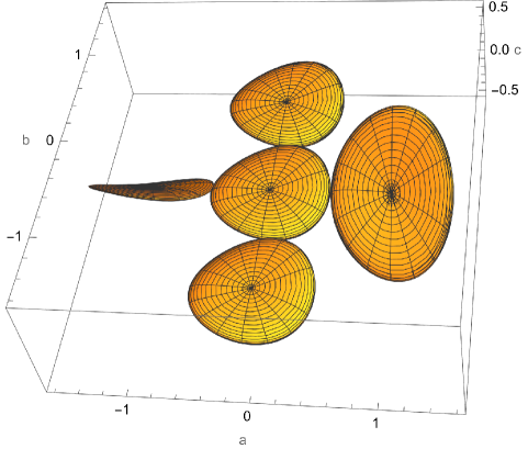
Figure 25: Sub-Riemannian balls $B_{1/2}(h)\subset G$ touching one another

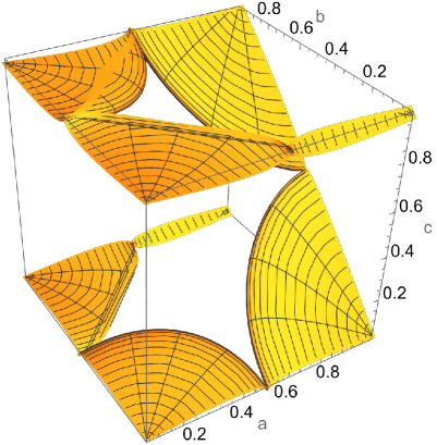
Figure 26: Sub-Riemannian ball $B^{\prime}_{1/2}\subset M$ touching itself

Remark 10.7

For the quotient of the Euclidean metric from $\mathbb{R}^{n}$ to $\mathbb{T}^{n}=\mathbb{R}^{n}/\mathbb{Z}^{n}$ (see Sec. 2) we have $\widehat{t}=\frac{1}{2}$ as well.

Theorem 10.8

We have

$$\sup\{t>0\mid\delta_{t}(E_{2})\cap h\delta_{t}(E_{2})=\emptyset\ \forall h\neq\operatorname{Id}\in H\}=\frac{1}{2}.$$

Proof.

Similarly to Theorem 10.6 since the ellipsoid $\delta_{t}(E_{2})$ is tangent to the sub-Riemannian sphere $B_{t}$ along the equator $B_{t}\cap\{z=0\}$. ∎

We plot the sets $h\delta_{1/2}(E_{2})$ for $h\in\{(0,0,0),(\pm 1,0,0),(0,\pm 1,0)\}$ in Fig. 27.

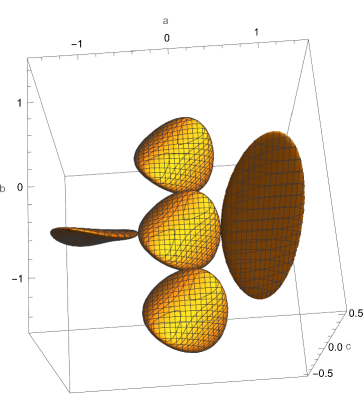
Figure 27: Sets $h\delta_{1/2}(E_{2})$ touching one another

Remark 10.9

Let $q(t)$ be a periodic sub-Riemannian geodesic in $M$ of period $T$. Then it is obvious that $t_{\operatorname{cut}}(q(\cdot))\leq\frac{T}{2}$ since $q(T/2)$ is a Maxwell point [10], i.e., an intersection point of two symmetric geodesics.

In a special case this bound turns into equality. Consider a geodesic $q(t)$ of the form $(\ref{c'})$ with $\theta=\frac{\pi n}{2}$, $n\in\mathbb{Z}$. Then it is easy to see that $t_{\operatorname{cut}}(q(\cdot))=\frac{T}{2}=\frac{1}{2}$.

11 Conclusion

This work seems to be the first study of a projection of a left-invariant sub-Riemannian structure on a Lie group to a compact homogeneous space. It reveals essential difference between the initial structure and its projection despite their local isometry.

For example, dynamical behaviour of sub-Riemannian geodesics on the Heisenberg group $G$ is trivial: all geodesics tend to infinity. Dynamics of sub-Riemannian geodesics on the Heisenberg 3D nil-manifold $M$ includes closed geodesics, dense in $M$ geodesics, and geodesics dense in a 2D torus.

Further, optimality of sub-Riemannian geodesics in $G$ is very well understood; the corresponding cut time arises due to continuous symmetries of the sub-Riemannian structure on $G$. Description of optimality and cut time on $M$ is much delicate since there are no continuous symmetries; and discrete symmetries which seem to generate the cut locus are hidden since they do not respect the projection mapping $\pi\,:\,G\to M$. Although, some two-sided bounds of the cut time in $M$ are possible due to two-sided bounds of sub-Riemannian balls and distance in $G$, which may be of independent interest.

References

- [1] R. Montgomery, A tour of subriemannnian geometries, their geodesics and applications, Amer. Math. Soc., 2002
- [2] A. Agrachev, D. Barilari, U. Boscain, A Comprehensive Introduction to sub-Riemannian Geometry from Hamiltonian viewpoint, Cambridge Studies in Advanced Mathematics, Cambridge Univ. Press, 2019
- [3] Agrachev A.A., Sachkov Yu.L., Control theory from the geometric viewpoint, Springer, 2004.
- [4] Arnold, V. I. Geometrical Methods in the Theory of Ordinary Differential Equations. Second edition. Grundlehren der Mathematischen Wissenschaften [Fundamental Principles of Mathematical Sciences], 250. Springer-Verlag, New York, 1988.
- [5] Bock, C. On low-dimensional solvmanifolds. Asian J. Math. 20 (2016), No. 2, 199–262.
- [6] Fomenko, A.; Fuchs, D. Homotopical topology. Second edition. Graduate Texts in Mathematics 273, Springer, 2016.
- [7] Furstenberg, H. Strict Ergodicity and Transformation of the Torus. Amer. J. Math. 83 (1961), No. 4, 573–601.
- [8] Katok, A.; Hasselblatt, B. Introduction to the modern theory of dynamical systems. Cambridge University Press, 1995.
- [9] Katok, A.; Hasselblatt, B. A first course in dynamics. Cambridge University Press, 2003.
- [10] Yu.Sachkov, Introduction to geometric control, Springer, 2022.
- [11] Yu.Sachkov, Left-invariant optimal control problems on Lie groups: classifications and problems integrable by elementary functions, Russian math. surveys, 77:1 (463) (2022), 109–176
- [12] Vinberg, È. B.; Gorbatsevich, V. V.; Shvartsman, O. V. Discrete subgroups of Lie groups. Current problems in mathematics. Fundamental directions, Vol. 21 (Russian), 5–120, 215 Itogi Nauki i Tekhniki [Progress in Science and Technology] Akad. Nauk SSSR, Vsesoyuz. Inst. Nauchn. i Tekhn. Inform., Moscow, 1988
- [13] Yu.Sachkov, Conjugate Time in the Sub-Riemannian Problem on the Cartan Group. J Dyn Control Syst 27, 709–751 (2021).
- [14] E. F. Sachkova, Sub-Riemannian balls on the Heisenberg group: an invariant volume, Journal of Mathematical Sciences, 199:5 (2014), 583–587