TimeAutoDiff: Combining Autoencoder and Diffusion model for time series tabular data synthesizing

Abstract

In this paper, we leverage the power of latent diffusion models to generate synthetic time series tabular data. Along with the temporal and feature correlations, the heterogeneous nature of the feature in the table has been one of the main obstacles in time series tabular data modeling. We tackle this problem by combining the ideas of the variational auto-encoder (VAE) and the denoising diffusion probabilistic model (DDPM). Our model named as TimeAutoDiff has several key advantages including (1) Generality: the ability to handle the broad spectrum of time series tabular data from single to multi-sequence datasets; (2) Good fidelity and utility guarantees: numerical experiments on six publicly available datasets demonstrating significant improvements over state-of-the-art models in generating time series tabular data, across four metrics measuring fidelity and utility; (3) Fast sampling speed: entire time series data generation as opposed to the sequential data sampling schemes implemented in the existing diffusion-based models, eventually leading to significant improvements in sampling speed, (4) Entity conditional generation: the first implementation of conditional generation of multi-sequence time series tabular data with heterogenous features in the literature, enabling scenario exploration across multiple scientific and engineering domains. Codes are in preparation for release to the public, but available upon request.

1 Introduction

Synthesizing tabular data is crucial for data sharing and model training. In the healthcare domain, synthetic data enables the safe sharing of realistic but non-sensitive datasets, preserving patient confidentiality while supporting research and software testing [40]. In fields like fraud detection [25, 11, 2], where anomalous events are rare, synthetic data can provide additional examples to train more effective detection models. Synthetic datasets are also vital for scenario exploration, missing data imputation [35, 24], and practical data analysis experiences across various domains.

Given the importance of synthesizing tabular data, many researchers have put enormous efforts into building tabular synthesizers with high fidelity and utility guarantees. For example, CTGAN [38] and its variants [44, 45] (e.g., CTABGAN, CTABGAN+) have gained popularity for generating tabular data using a Generative Adversarial Networks [4] (GANs). Recently, diffusion-based tabular synthesizers, like Stasy [13], have shown promise, outperforming GAN-based methods in various tasks. Yet, diffusion models [7, 32] were not initially designed for heterogeneous features. New approaches, such as those using Doob’s h-transform [22], TabDDPM [15], and CoDi [17], aim to address this challenge by combining different diffusion models [32, 10] or leveraging contrastive learning [29] to co-evolve models for improved performance on heterogeneous data. Most recently, researchers have used the idea of latent diffusion model, i.e., AutoDiff [34] and TabSyn [42], to model the heterogeneous features in tables, and prove its empirical effectiveness in various tabular generation tasks.

However, the tabular synthesizers mentioned above focus solely on generating tables with independent and identically distributed (i.i.d.) rows. They face difficulties in simulating time series tabular data due to the significant inter-dependences among features and the intricate temporal dependencies that unfold over time. Motivated from [34, 42], we propose a new model named TimeAutoDiff, which combines Variational Auto-encoder (VAE) [14] and Denoising Diffusion Probabilistic Model (DDPM) [7] to tackle the above challenges in time series tabular modeling. In the rest of this section, we will specify our problem formulation, challenges, and contributions of our work.

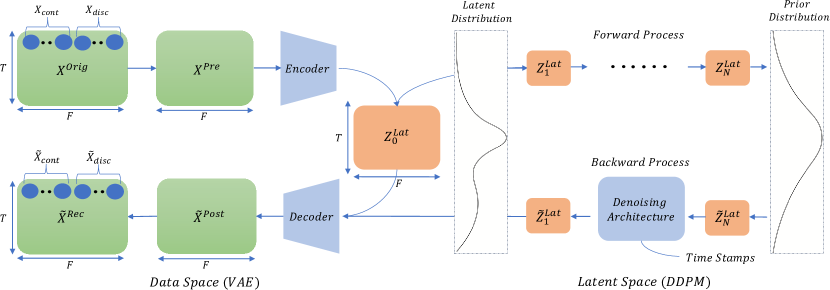
Figure 1: The overview of TimeAutoDiff: the model has three components: (1) pre- and post-processing steps for the original and synthesized data, respectively; (2) VAE for training encoder and decoder, and for projecting the pre-processed data to the latent space; (3) Diffusion model for learning the distribution of projected data in latent space and generating new latent data. Note that the dimension of the latent matrix $Z_{0}^{\text{Lat}}\in\mathbb{R}^{T\times F}$ is set to be the same as that of the original data.

1.1 Problem Formulation, Challenges, and Contributions

Our goal is to learn the joint distribution of time series tabular data of a $T$-sequence $(\mathbf{x}_{1},\dots,\mathbf{x}_{T})$. Each observation $\mathbf{x}_{j}$, where $\mathbf{x}_{j}:=[\mathbf{x}_{\text{Cont},j},\mathbf{x}_{\text{Disc},j}]$ consists of a $F$-dimensional feature vector that includes both continuous ($\mathbf{x}_{\text{Cont},j}$) and discrete variables ($\mathbf{x}_{\text{Disc},j}$), reflecting the heterogeneous nature of the dataset. Throughout this paper, we assume there are $B$ i.i.d. observed sequences sampled from $\mathbb{P}(\mathbf{x}_{1},\dots,\mathbf{x}_{T})$. We additionally assume that each record in the time-series tabular data includes a timestamp, formatted as ’YEAR-MONTH-DATE-HOURS’. This timestamp serves as an auxiliary variable to aid an inference step in TimeAutoDiff, which will be detailed shortly.

The overview of TimeAutoDiff is provided in Figure 1. Inspired from [34, 42], we take advantage of the latent diffusion model [28]. Our model has two inference stages: (I). training of VAE [14] to project the time series data to latent spaces; (II). training of DDPM [7] to learn the latent distribution of projected time series data. This seemingly simple idea of combining two powerful models resolves several challenges in time series tabular data modeling.

Heterogeneous features pose a significant challenge in tabular data synthesis, as real-world tables often contain a mix of continuous, discrete, or other types of features [44, 45]. We utilize a Variational Autoencoder (VAE) to encode these heterogeneous features into continuous representations in a latent space. The VAE reconstructs the original input and generates new data points. We then use a diffusion model to generate new latent representations from the learned continuous representations. Finally, the trained decoder converts these new representations back into the original heterogeneous feature format. This approach combines the strengths of both models: VAE’s ability to handle heterogeneous features and the diffusion model’s effectiveness in learning distributions in continuous spaces.

Feature and temporal correlations are important statistical objects that need to be captured when building a time series tabular synthesizer. Yet, due to the heterogeneous nature of tabular data, capturing these correlations is even more demanding than capturing correlations among purely continuous or discrete features. TimeAutoDiff naturally circumvents this challenge by its construction as the diffusion model learns the distribution of latent representations jointly in the continuous space. As long as VAE gives good latent representations of rows in the table, it should be expected that TimeAutoDiff can nicely capture both temporal and feature correlations in the table. Specifically, the encoder in VAE employs $1$-layer transformer [37] to capture feature correlations and Recurrent Neural Network (RNN) [9] to model the temporal dependences of sequences. In Section 4, we empirically verify that TimeAutoDiff indeed captures both correlations well when compared with other State-Of-The-Art (i.e., SOTA) time series tabular synthesizers.

Sampling time for new data sequence generation is reduced significantly when compared with other SOTA diffusion-based time series models, including TSGM [20] and diffusion-ts [41], which are all sequential sampling-based methods. The existing synthesizers are typically designed to model the conditional distribution $\mathbb{P}(\mathbf{x}_{t}|\mathbf{x}_{t-1},\dots,\mathbf{x}_{1})$ over $t\in\{2,\dots,T\}$ and generate $\mathbf{x}_{t}$ sequentially. In contrast, our model learns the entire distribution of the sequence (i.e., $\mathbb{P}(\mathbf{x}_{T},\mathbf{x}_{T-1},\dots,\mathbf{x}_{1})$), and generates the whole sequence at one time. This approach also has the auxiliary advantage of circumventing the accumulating errors associated with sequential sampling methods.

Multi-sequence tabular data, with multiple sequences from various entities, is common in many real-world datasets. In our work, this data consists of $B$ entities with sequential data of size $\mathbb{R}^{T\times F}$, assuming each entity shares the same time series distribution $\mathbb{P}(\mathbf{x}_{1},\dots,\mathbf{x}_{T})$. Our model uniquely performs entity conditional generation of multi-sequence data with heterogeneous features (see Table 1). Given an entity label $\mathbf{e}_{i}$, $\forall i\in{1,\dots,B}$, it samples from the conditional distribution $\mathbb{P}(\mathbf{x}_{1},\dots,\mathbf{x}_{T}\mid\mathbf{e}_{i})$ using classifier-free guidance in diffusion models. This is achieved through the TimeAutoDiff framework, which combines autoencoder and diffusion models, surpassing current SOTA models in handling the joint distribution of heterogeneous features.

Numerical comparisons of TimeAutoDiff with other models (with publicly available codes), namely, TimeGAN [39], Diffusion-ts [41], TSGM [19], CPAR [43], and DoppelGANger [21] are conducted comprehensively across six real-world datasets under various metrics. Specifically, qualities of generated tables are measured through (1) statistical fidelities to real tables, (2) machine learning utilities in downstream tasks, and (3) sampling times. Specifically, for measuring the fidelities of temporal correlations between synthetic and real heterogeneous timeseries tabular data, we develop a new metric, named Temporal Discriminative Score. Inspired from the paper [39, 43], this metric computes discriminative scores [39] of distributions of inter-row differences [43] in generated and original sequential data. More details will be presented in Section 4.

In Table 1, we summarize the contributions of our model by comparing ours with the SOTA time series synthesizers in the literature under various metrics. Concise descriptions of each model in Table 1 and relevant literature are provided in the following subsection.

1.2 Relevant Literature

To our knowledge, not many models in literature can deal with time series tabular data with a heterogeneous nature. We categorize the incomplete list of existing models into three parts: (1) GAN-based models, (2) Diffusion-based models, and (3) GPT-based / Parametric models.

GAN-based models. TimeGAN [39] is one of the most popular time series data synthesizers based on GAN framework. Notably, they used the idea of latent GAN employing the auto-encoder for projecting the time series data to latent space and model the distribution of the data in latent space through GAN framework. Recently proposed Electric Health Record (in short EHR)-Safe [40] integrates a GAN with an encoder-decoder module to generate realistic time series and static variables in EHRs with mixed data types, while EHR-M-GAN [18] employs distinct encoders for each data type, enhancing the generation of mixed-type time series in EHRs. Despite these advancements, GAN-based methods still encounter challenges such as non-convergence, mode collapse, generator-discriminator imbalance, and sensitivity to hyperparameter selection, underscoring the need for ongoing refinement in time series data synthesis.

Diffusion-based models. Most recently, TimeDiff [36], which adopts the idea from TabDDPM combining the multinomial and Gaussian diffusion models to generate a synthetic EHR time series tabular dataset, appeared on arXiv but without publicly available code. DPM-EHR [16] suggested another diffusion-based mixed-typed EHR time series synthesizer, which mainly relies on Gaussian diffusion and U-net architecture. TSGM [19] used the idea of the latent conditional score-based diffusion model to generate continuous time series data. However, TSGM is highly overparameterized and its training, inference, and sampling steps are quite slow. Diffusion-ts [41] takes advantage of the latent diffusion model employing transformer-based auto-encoder to capture the temporal dynamics of complicated time series data. Specifically, they decompose the seasonal-trend components in time series data making the generated data highly interpretable. One important model in the literature, CSDI [35], uses a 2D-attention-based conditional diffusion model to impute the missing continuous time series data. However, our work focuses on heterogeneous time series tabular data generation and we leave the missing data imputation as future work.

GPT-based / Parametric models. TabGPT [25] is a GPT2-based tabular data synthesizer, which can deal with both single and multi-sequence mixed-type time series datasets. Data generation of TabGPT is performed by first inputting initial rows of data, then generating synthetic rows based on the context of previous rows. However, from our own experiences, the codes provided by the authors only work for credit card transaction dataset with some flawed outputs. CPAR [43] is an autoregressive model designed for synthesizing multi-sequence tabular data. They use different parametric models (i.e., Gaussian, Negative Binomial) for modeling different datatypes (i.e., continuous, discrete). However, this independent parametric design of each feature ignores capturing correlations among the features, which is an important task in tabular synthesizing.

Models Hetero. Single-Seq. Multi-Seq. Entity Gen. Applicability Code Sampling Time TimeAutoDiff ✓ ✓ ✓ ✓ ✓ ✓ $3$ TimeDiff [36] ✓ ✓ ✗ ✗ ✗ ✗ – Diffusion-ts [41] ✗ ✓ ✗ ✗ ✓ ✓ $5$ TSGM [20] ✗ ✓ ✗ ✗ ✓ ✓ $6$ TimeGAN [39] ✗ ✓ ✗ ✗ ✓ ✓ $2$ DoppelGANger [21] ✗ ✓ ✗ ✗ ✓ ✓ $1$ EHR-M-GAN [18] ✓ ✓ ✗ ✗ ✗ ✓ – CPAR [43] ✓ ✗ ✓ ✗ ✓ ✓ $4$ TabGPT [25] ✓ ✗ ✓ ✗ ✗ ✓ –

Table 1: A comparison table that summarizes TimeAutoDiff against baseline methods, evaluating metrics like heterogeneity, single- and multi-sequence data generation, entity conditional generation, applicability (i.e., whether the model is not designed for specific domains), code availability, and sampling time. Baseline models without domain specificity and with available code are used for numerical comparisons. The sampling time column ranks models by their speed, with lower numbers indicating faster sampling. More details can be found in Table 2.

2 Proposed Model

In this section, we provide detailed descriptions of each component within our model. Pre- and post-processing steps of the input and synthesized tabular data are introduced. Then, the constructions on variational auto-encoder (VAE) and diffusion models are provided.

Pre- and post-processing steps. It is essential to pre-process the real tabular data in a form that the machine learning model can extract the desired information from the data properly. We divide the heterogeneous features into two categories; (1) continuous, and (2) discrete. Following is how we categorize the variables and process each feature type. Let $\mathbf{x}$ be the column of a table to be processed.

1. Continuous feature: If $\mathbf{x}$’s entries are real-valued continuous, we categorize $\mathbf{x}$ as a numerical feature. Moreover, if the entries are integers with more than $25$ distinct values (e.g.,“Age”), then $\mathbf{x}$ is categorized as a continuous variable. Here, $25$ is a user-specified threshold. We employ min-max scaler [39] to ensure the pre-processed numerical features are within the range of $[0,1]$. Hereafter, we denote $\mathbf{x}^{\text{Proc}}_{\text{Cont}}$ as the processed column.

2. Discrete / Categorical feature: If $\mathbf{x}$’s entries have string datatype, we categorize $\mathbf{x}$ as a discrete feature (e.g., “Gender”). Additionally, the $\mathbf{x}$ with less than $25$ distinct integers is categorized as a discrete feature. For pre-processing, we simply map the entries of $\mathbf{x}$ to the integers greater than or equal to $0$, and further divide the data type into two parts; binary and categorical, denoting them as $\mathbf{x}^{\text{Proc}}_{\text{Bin}}$ and $\mathbf{x}^{\text{Proc}}_{\text{Cat}}$.

3. Post-processing step: After the TimeAutoDiff model generates a synthetic dataset, it must be restored to its original format. For continuous features, this is achieved through inverse transformations, (i.e., reversing min-max scaling). Integer labels in discrete features are mapped back to their original categorical or string values.

Variational Auto-Encoder. The pre-processed input data $\mathbf{x}^{\text{Proc}}:=[\mathbf{x}^{\text{Proc}}_{\text{Bin}};\mathbf{x}^{\text{Proc}}_{\text{Cat}};\mathbf{x}^{\text{Proc}}_{\text{Cont}}]\in\mathbb{R}^{B\times T\times F}$ is fed into the VAE. The architecture of the encoder is illustrated in Figure 2. Motivated by TabTransformer [12], we encode the discrete features $\mathbf{x}_{\text{Disc}}:=[\mathbf{x}^{\text{Proc}}_{\text{Bin}};\mathbf{x}^{\text{Proc}}_{\text{Cat}}]=\{\mathbf{x}_{1},\dots,\mathbf{x}_{m}\}$ into a $d$-dimensional (where $d$ is consistently set at $128$ in this paper) continuous representation. This is achieved using a lookup table $\mathbf{e}(\cdot)\in\mathbb{R}^{d}$, referred to as the column feature, with $m$ representing the total number of discrete features.

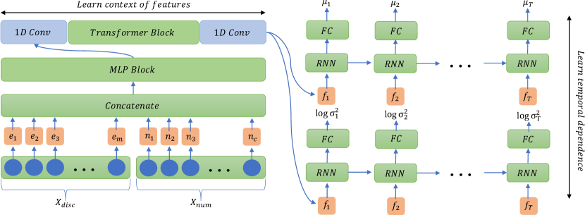
Figure 2: The schematic architecture of the encoder in VAE.

The goal of introducing embedding for the discrete variables is to allow the model to differentiate the classes in one column from those in the other columns. To embed the continuous features, we employ a frequency-based representation. Let $\nu$ be a scalar value of the $j$-th continuous feature in $\mathbf{x}_{\text{Cont}}^{\text{Proc}}$. Similarly with [23], $\nu$ is projected to the embedding spaces as follows:

$$n_{j}(\nu):=\text{Linear}\big{(}\text{SiLU}\big{(}\text{Linear}\big{(}[\text{sin}(2^{0}\pi\nu),\text{cos}(2^{0}\pi\nu),\cdots,\text{sin}(2^{7}\pi\nu),\text{cos}(2^{7}\pi\nu)]\big{)}\big{)}\big{)}\in\mathbb{R}^{d}.$$ (1)

The embedding dimensions of discrete and continuous features are set to be the same as $d$ for simplicity. The sinusoidal embedding in (1) plays a crucial role in reconstructing the heterogeneous features. Our empirical observations indicate that omitting this embedding degrades the reconstruction fidelity of continuous features compared to their discrete counterparts, which will be verified in the ablation test in the following section. As noted in [23], we conjecture this is attributed to the fact that deep networks are biased towards learning the low-frequency functions (i.e., spectral bias [27]), while the scaler values in continuous time series features often have higher frequency variations.

The embedded vectors $\{e_{1},\dots,e_{m},n_{1},\dots,n_{c}\}$ are concatenated into a vector of dimension $(m+c)d$, input to the MLP block (2) whose output has the same shape with that of the input tensor $[B,T,F]$. Then, we employ the technique used in CSDI [35] to learn the context of features via the 1D-convolutional layer and attention mechanism. Through the convolution layer, the tensor is projected to $4D$ space $[B,C,T,F]$ with $C$ denoting the number of channels. The reshaped tensor of $[BT,C,F]$ is fed to the Transformer encoder block in [37] to learn the context of features, outputting the tensor of the same size. After going through another convolutional layer and reshaping, the output tensor $[f_{1}^{(i)},f_{2}^{(i)},\dots,f_{T}^{(i)}]_{i=1}^{B}\in\mathbb{R}^{B\times T\times F}$ is fed to two RNN blocks. Hereafter, we omit the notation for batch index, when it is clear from context.

These two RNN blocks learn the temporal dependences of features, outputting $\mathbf{\mu}:=[\mu_{1},\mu_{2},\dots,\mu_{T}]^{T}\in\mathbb{R}^{T\times F}$ and $\mathbf{\log\sigma^{2}}:=[\log\sigma_{1}^{2},\log\sigma_{2}^{2},\dots,\log\sigma_{T}^{2}]^{T}\in\mathbb{R}^{T\times F}$, respectively. Then, we have latent embedding tensors $\mathbf{Z}^{\text{Lat}}:=\mathbf{\mu}+\mathbf{\epsilon}\mathbf{\sigma}\in\mathbb{R}^{T\times F}$, where $\mathbf{\epsilon}$’s each entry is from standard Gaussian distribution. The size of $\mathbf{Z}^{\text{Lat}}$ is set to be the same as that of the input tensor through fully-connected (FC) layers topped on the output of two RNN blocks. We found a simple MLP block and FC layers work well as a decoder in our VAE.

Specifically, we first apply MLP to $\mathbf{Z}^{\text{Lat}}$ as in (2):

$$\text{MLPBlock}(\mathbf{x}):=\text{Linear}(\text{ReLU}(\text{Linear}(\mathbf{x}))),\quad\mathbf{x}^{\text{Pre-Out}}=\text{MLPBlock}(\mathbf{Z}^{\text{Lat}}).$$ (2)

Then, FC layers are applied to $\mathbf{x}^{\text{Pre-Out}}$ for each of data types; that is, $\mathbf{x}^{\text{Out}}_{\text{Cont}}:=\text{Sigmoid}(\text{Linear}(\mathbf{x}^{\text{Pre-Out}}))$, $\mathbf{x}^{\text{Out}}_{\text{Bin}}:=\text{Linear}(\mathbf{x}^{\text{Pre-Out}})$, and $\mathbf{x}^{\text{Out}}_{\text{Cat}}:=\text{Linear}(\mathbf{x}^{\text{Pre-Out}})$, denoting continuous, binary, and categorical outputs of the decoder, respectively. Note that for numerical features, sigmoid activation function is taken to match the scale of $\mathbf{x}^{\text{Proc}}_{\text{Cont}}\in[0,1]$. The dimensions of $\mathbf{x}^{\text{Out}}_{\text{Cont}}$ and $\mathbf{x}^{\text{Out}}_{\text{Bin}}$ are the same as their corresponding inputs, but the dimension of $\mathbf{x}^{\text{Out}}_{\text{Cat}}$ is $\sum_{i}K_{i}$ where $K_{i}$ is the number of categories in each categorical variable. We set the dimensions of output features in this way as we used the mean-squared (MSE), binary cross entropy (BCE), and cross-entropy (CE) in Pytorch package. The reconstruction error is defined as:

$$\ell_{\text{recons}}(\mathbf{x}^{\text{Proc}},\mathbf{x}^{\text{Out}})=\text{MSE}(\mathbf{x}^{\text{Proc}}_{\text{Cont}},\mathbf{x}^{\text{Out}}_{\text{Cont}})+\text{BCE}(\mathbf{x}^{\text{Proc}}_{\text{Bin}},\mathbf{x}^{\text{Out}}_{\text{Bin}})+\text{CE}(\mathbf{x}^{\text{Proc}}_{\text{Cat}},\mathbf{x}^{\text{Out}}_{\text{Cat}}).$$ (3)

Following [5, 42], we use $\beta$-VAE [6] instead of ELBO loss, where a coefficient $\beta(\geq 0)$ balances between the reconstruction error and KL-divergence of $\mathcal{N}(0,\mathcal{I})$ and $\mathbf{z}^{\text{Lat}}\sim\mathcal{N}(\mathbf{\mu},\mathbf{\sigma^{2}})$.

Finally, we minimize the following objective function $\mathcal{L}_{\text{Auto}}$ for training VAE:

$$\mathcal{L}_{\text{Auto}}:=\ell_{\text{recons}}(\mathbf{x}^{\text{Proc}},\mathbf{x}^{\text{Out}})+\beta\mathcal{D}_{\textbf{KL}}\big{(}\mathcal{N}(\text{vec}(\mathbf{\mu}),\text{diag}(\text{vec}(\mathbf{\sigma^{2}})))\mid\mid\mathcal{N}(0,\mathcal{I}_{TF\times TF})\big{)}.$$ (4)

Similar as in [42], our model does not require the distribution of embeddings $\mathbf{z}^{\text{Lat}}$ to follow a standard normal distribution strictly as the diffusion model additionally handle the distributional modeling in the latent space. Following [42], we adopt the adaptive schedules of $\beta$ with its maximum value set as $0.1$ and minimum as $10^{-5}$, decreasing the $\beta$ by a factor of $0.7$ (i.e., $\beta^{\text{new}}=0.7\beta^{\text{old}}$) from maximum to minimum whenever $\ell_{\text{recons}}$ fails to decrease for a pre-defined number of epochs.

Diffusion for Time Series. TimeAutoDiff is designed to generate the entire time series at once, taking the data of shape $T\times F$ as an input. This should be contrasted to generating rows in the table sequentially (i.e., for instance [20]). We extend the idea of DDPM to make it accommodate the 2D input. For readers’ convenience, we provide an overview of DDPM in Appendix C.

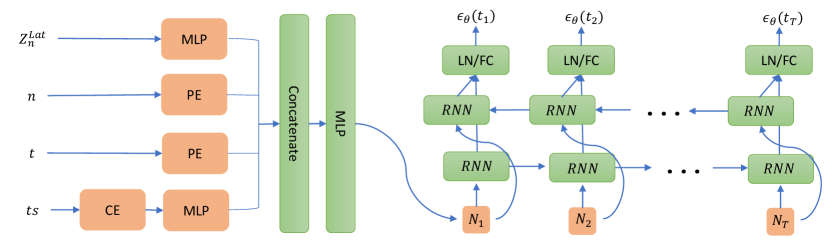
Figure 3: The schematic architecture of the $\epsilon_{\theta}(\mathbf{Z}_{n}^{\text{Lat}},n,\mathbf{t},\textbf{ts})$ in diffusion model.

Let $\mathbf{Z}^{\text{Lat}}_{0}\in\mathbb{R}^{T\times F}$ denote the input latent matrix from VAE and let $\mathbf{Z}^{\text{Lat}}_{n}:=[\mathbf{z}^{\text{Lat}}_{n,1},\mathbf{z}^{\text{Lat}}_{n,2},\dots,\mathbf{z}^{\text{Lat}}_{n,F}]$ be the noisy matrix after $n$ diffusion steps, where $\mathbf{z}^{\text{Lat}}_{n,j}\in\mathbb{R}^{T}$ is the $j$-th column of $\mathbf{Z}^{\text{Lat}}_{n}$. The perturbation kernel $q(\mathbf{z}_{n,j}^{\text{Lat}}|\mathbf{z}_{0,j}^{\text{Lat}})=\mathcal{N}(\sqrt{\bar{\alpha}_{n}}\mathbf{z}_{0,j}^{\text{Lat}},(1-\bar{\alpha}_{n})\mathcal{I}_{T\times T})$ is applied independently to each column $\mathbf{z}^{\text{Lat}}_{0,j}$ $j\in[F]$, where $\bar{\alpha_{n}}:=\Pi_{i=1}^{n}\alpha_{i}$ with $\{\alpha_{i}\}_{i=1}^{n}\in[0,1]^{n}$ being a decreasing sequence over $i$. Here, we treat each column of $\mathbf{Z}^{\text{Lat}}_{0}$ as a discretized measurement of univariate time series function in the latent space, adding noises independently. But, as noted in [1], this does not mean we do not model the correlations along the feature dimension in $\mathbf{Z}^{\text{Lat}}_{0}$. The reverse process for sampling takes an entire latent matrix and captures these correlations. A similar idea has been used in TabDDPM [15] for modeling categorical variables. Under this setting, $\mathbf{Z}^{\text{Lat}}_{n}$ can be succinctly written as $\sqrt{\bar{\alpha}_{n}}\mathbf{Z}_{0}^{\text{Lat}}+\sqrt{1-\bar{\alpha}_{n}}\mathbf{E}^{n}$, where $\mathbf{E}^{n}:=[\epsilon_{1}^{n},\epsilon_{2}^{n},\dots,\epsilon_{F}^{n}]\in\mathbb{R}^{T\times F}$. Here, $\epsilon_{j}^{n}\sim\mathcal{N}(0,\mathcal{I}_{T\times T})$ denotes noises.

Finally, the ELBO loss we want to aim to minimize is:

$$\mathcal{L}_{\text{diff}}:=\mathbb{E}_{n,\mathbf{E}^{n}}\big{[}\|\mathbf{\epsilon}_{\theta}\big{(}\sqrt{\bar{\alpha}_{n}}\mathbf{Z}_{0}^{\text{Lat}}+\sqrt{1-\bar{\alpha}_{n}}\mathbf{E}^{n},n,\mathbf{t},\mathbf{ts}\big{)}-\mathbf{E}^{n}\|_{2}^{2}\big{]}.$$ (5)

The neural network $\epsilon_{\theta}$ predicts the error matrix $\mathbf{E}^{n}$ added in every diffusion step $n\sim\text{Unif}(\{1,2,\dots,N\})$. It takes noisy matrix $\mathbf{Z}^{\text{Lat}}_{n}$, normalized time-stamps $\mathbf{t}:=\{t_{1},t_{2},\dots,t_{T}\}\subset[0,1]^{T}$, diffusion step $n$, and the original time-stamps $\mathbf{ts}$ in the tabular dataset as inputs. The architecture of $\epsilon_{\theta}$ is given in Fig. 2. Diffusion step $n$ and a set of normalized time points $\mathbf{t}$ are encoded through positional encoding (in short PE) introduced in [37]. PE of $n$ lets the diffusion model know at which diffusion step the noisy matrix is, and PE of $\mathbf{t}$ encodes the sequential order of rows in the input matrix. But normalized time stamps provide only limited information on the orders of rows, and we find incorporating the encodings of timestamps in date-time format (i.e., YEAR-MONTH-DATE-HOURS), which can be commonly found in time series tabular data, significantly helps the diffusion training process. Cyclic encodings with sine and cosine functions are used for converting the date-time data to dense vectors: specifically, for $\mathbf{x}\in\{\text{YEAR},\text{MONTH},\text{DATE},\text{HOURS}\}$ with $\text{Period}\in\{\text{total number of years in the dataset},12,365,24\}$, the conversion we used is as follows:

$$\big{(}\text{sin}\big{(}\mathbf{x}/(\text{Period}\times 2\pi)\big{)},\text{cos}\big{(}\mathbf{x}/(\text{Period}\times 2\pi)\big{)}\big{)}.$$ (6)

Through (6), cyclic encodings give $16$-dimensional unique representations of timestamps of observed data in the table, and the encoded vector is fed to an MLP block (2) to match the dimension with those of the other inputs’ encodings. The concatenated encodings of ($Z_{n}^{\text{Lat}}$, $\mathbf{n}$, $\mathbf{t}$, ts) are fed into a MLP block, which gives a tensor $\mathbf{N}=[N_{1},N_{2},\dots,N_{T}]^{T}\in\mathbb{R}^{T\times F}$. Inspired from [36], Bi-directional RNN (BRNN) [30] is employed and $\mathbf{N}$ is fed to BRNN as in Figure 2. After the applications of layer-normalization and FC layer, the network $\epsilon_{\theta}$ outputs $[\epsilon_{\theta}(t_{1}),\dots,\epsilon_{\theta}(t_{T})]^{T}\in\mathbb{R}^{T\times F}$ to estimate $\mathbb{E}^{n}$. The sampling process of new latent matrix is deferred to the Appendix D.

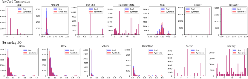
Figure 4: Plots of marginal distributions of real versus synthetic data: (a) card transaction, (b) nasdaq100. The synthetic data are generated “conditionally” on labels of entities from each dataset.

3 Entity Conditional Generation

TimeAutoDiff is capable of accommodating the entity conditional generation in multi-sequence tabular data. This feature is attributed to the unique capability of diffusion model for conditional generations via classifier-free guidance [8] technique. First, the integer labels (i.e., lbl) of the entities (e.g., Stock symbols in nasdaq100 dataset, APPL : 0, MSFT : 1) are encoded to continuous space via the lookup table. After going through the MLP block, the encoded labels are added to the encodings of diffusion step $n$. We denote this label conditioned model as $\mathbf{\epsilon}_{\theta}\big{(}\mathbf{Z}_{n}^{\text{Lat}},n,\mathbf{t},\mathbf{ts},\mathbf{lbl}\big{)}$. Following [8], we jointly train the conditional and unconditional models by randomly setting lbl as the unconditional class identifier $\emptyset$ with some pre-specified probability. (throughout this paper, we set it as $0.1$.) We use a single neural network to parameterize both models. After training, we perform sampling using the following linear combination of the conditional and unconditional noise estimates:

$$\tilde{\epsilon}_{\theta}:=(1+\omega)\cdot\mathbf{\epsilon}_{\theta}\big{(}\mathbf{Z}_{n}^{\text{Lat}},n,\mathbf{t},\mathbf{ts},\mathbf{lbl}\big{)}-\omega\cdot\mathbf{\epsilon}_{\theta}\big{(}\mathbf{Z}_{n}^{\text{Lat}},n,\mathbf{t},\mathbf{ts},\mathbf{lbl}=\emptyset\big{)},$$ (7)

where the $\omega$ controls the strength of guidance of the implicit classifier. (We set $\omega=3$ in this work.)

The detailed algorithm for sampling is deferred in Appendix D. For the visual demonstrations of our results, in Figure 4, we plot the marginal distributions of real versus synthetic of card transaction and nasdaq100 datasets. We give the model the labels of the entire entities in each dataset, and the model generates the sequences of corresponding labels. We refer to the model as C-TimeAutoDiff. (Here, the letter ‘C’ stands for conditional.) For numerical comparisons, we evaluate the performance of entity conditional generation using our C-TimeAutoDiff model against baseline models (CPAR, TimeGAN, DoppelGANger, TSGM) and our model TimeAutoDiff through unconditional generation.

4 Numerical Experiments

In this section, we evaluate our TimeAutoDiff model in two modes: unconditional and conditional generation, in order to verify the quality of generated time series tabular data. To conduct comparative studies, we choose $5$ baseline models: TimeGAN [39], Diffusion-TS [41], TSGM [19], CPAR [43], and DoppelGANger [21]. We use 6 publicly available datasets where Traffic, Pollution, Hurricane, AirQuality are single-sequence data, and card transaction and nasdaq100 are multi-sequence data. Brief introductions of each dataset with the links for the sources are deferred to Appendix A.

4.1 Metrics for Evaluations

For quantitative evaluation of synthesized data, we mainly focus on three criteria (1) distributional similarities of two tables; (2) the usefulness for predictive purposes; (3) the temporal and feature dependencies; We employ the following evaluation metrics:

1. Discriminative Score [39] measures the fidelity of synthetic time series data to original data, by training a classification model (optimizing a 2-layer LSTM) to distinguish between sequences from the original and generated datasets.

2. Predictive Score [39] measures the utility of generated sequences by training a posthoc sequence prediction model (optimizing a 2-layer LSTM) to predict next-step temporal vectors under Train-on-Synthetic-Test-on-Real (TSTR) framework.

3. Temporal Discriminative Score measures the similarity of distributions of inter-row differences between generated and original sequential data. This metric is designed to see if the generated data preserves the temporal dependences of the original data. For any fixed integer $t\in\{1,\dots,T-1\}$, the difference of $n$-th row and $(n+t)$-th row in the table over $n\in\{1,\dots,T-t\}$ is computed for both generated and original data, and discriminative score [39] is computed over the differenced matrices from original and synthetic data. We average discriminative scores over $10$ randomly selected $t\in\{1,\dots,T-1\}$.

4. Feature Correlation Score measures the averaged $L^{2}$-distance of correlation matrices computed on real and synthetic data. Following [15], to compute the correlation matrices, we use the Pearson correlation coefficient for numerical-numerical feature relationships, Theil’s U statistics between categorical-categorical features, and the correlation ratio for categorical-numerical features. For readers’ convenience, we provide the definitions of these three metrics in Appendix E.

Metric Methods Single-Sequence Multi-Sequence Traffic Pollution Hurricane AirQuality Card Transaction nasdaq100 Sampling Time (in Sec) (The lower, the better) TimeAutoDiff C-TimeAutoDiff Diffusion-ts TSGM TimeGAN DoppelGANger CPAR 3.512 (0.065) N.A. $\gg$ $\gg$ $0.127(0.056)$ $\mathbf{0.011(0.002)}$ $17.466(0.734)$ 3.947 (0.070) N.A. $\gg$ $\gg$ $0.113(0.058)$ $\mathbf{0.014(0.001)}$ $18.597(0.558)$ 3.740 (0.132) N.A. $\gg$ $\gg$ $0.125(0.060)$ $\mathbf{0.010(0.003)}$ $15.839(0.324)$ 3.945 (0.103) N.A. $\gg$ $\gg$ $0.131(0.060)$ $\mathbf{0.017(0.003)}$ $29.816(0.846)$ $3.384(0.064)$ $7.209(1.697)$ N.A. N.A. $0.051(0.051)$ $\mathbf{0.018(0.004)}$ $141.425(2.435)$ $3.133(0.129)$ $5.888(0.131)$ N.A. N.A. $0.047(0.039)$ $\mathbf{0.041(0.001)}$ $112.506(2.152)$ Discriminative Score (The lower, the better) TimeAutoDiff C-TimeAutoDiff Diffusion-ts TSGM TimeGAN DoppelGANger CPAR Real Data $\mathbf{0.026(0.014)}$ N.A. $0.202(0.021)$ $0.500(0.000)$ $0.413(0.057)$ $0.258(0.215)$ $0.498(0.002)$ $0.053(0.009)$ $\mathbf{0.016(0.009)}$ N.A. $0.133(0.015)$ $0.488(0.010)$ $0.351(0.053)$ $0.100(0.103)$ $0.500(0.000)$ $0.048(0.017)$ $\mathbf{0.047(0.016)}$ N.A. $0.181(0.018)$ $0.482(0.020)$ $0.254(0.062)$ $0.176(0.099)$ $0.500(0.000)$ $0.034(0.011)$ $\mathbf{0.061(0.013)}$ N.A. $0.134(0.016)$ $0.452(0.009)$ $0.460(0.020)$ $0.211(0.116)$ $0.499(0.001)$ $0.040(0.011)$ $\mathbf{0.215(0.058)}$ $0.257(0.055)$ N.A. N.A. $0.482(0.037)$ $0.485(0.025)$ $0.500(0.000)$ $0.225(0.094)$ $\mathbf{0.067(0.046)}$ $0.138(0.040)$ N.A. N.A. $0.267(0.115)$ ${0.071(0.032)}$ $0.143(0.120)$ $0.190(0.051)$ Predictive Score (The lower, the better) TimeAutoDiff C-TimeAutoDiff Diffusion-ts TSGM TimeGAN DoppelGANger CPAR Real Data $\mathbf{0.203(0.014)}$ N.A. $0.231(0.007)$ $0.247(0.002)$ $0.297(0.008)$ $0.300(0.005)$ $0.263(0.003)$ $0.206(0.012)$ $\mathbf{0.008(0.000)}$ N.A. $0.013(0.000)$ $0.009(0.000)$ $0.043(0.000)$ $0.282(0.028)$ $0.032(0.009)$ $0.010(0.000)$ $\mathbf{0.098(0.026)}$ N.A. $0.306(0.076)$ $0.290(0.007)$ $0.180(0.027)$ $0.214(0.000)$ $0.420(0.055)$ $0.098(0.026)$ $\mathbf{0.005(0.001)}$ N.A. $0.017(0.002)$ $0.006(0.000)$ $0.057(0.011)$ $0.060(0.009)$ $0.030(0.007)$ $0.005(0.001)$ $\mathbf{0.001(0.000)}$ $\mathbf{0.001(0.000)}$ N.A. N.A. $0.130(0.022)$ $0.004(0.006)$ $0.132(0.035)$ $0.001(0.000)$ $10.863(0.716)$ $9.285(0.034)$ N.A. N.A. $9.597(0.016)$ $11.556(1.093)$ $\mathbf{8.270(0.019)}$ $9.281(0.009)$ Temporal Discriminative Score (The lower, the better) TimeAutoDiff C-TimeAutoDiff Diffusion-ts TSGM TimeGAN DoppelGANger CPAR Real Data $\mathbf{0.047(0.018)}$ N.A. $0.199(0.028)$ $0.499(0.001)$ $0.429(0.050)$ $0.400(0.039)$ $0.436(0.073)$ $0.061(0.011)$ $\mathbf{0.014(0.013)}$ N.A. $0.165(0.084)$ $0.499(0.001)$ $0.397(0.060)$ $0.444(0.050)$ $0.492(0.021)$ $0.044(0.009)$ $\mathbf{0.026(0.024)}$ N.A. $0.247(0.093)$ $0.497(0.002)$ $0.465(0.025)$ $0.464(0.028)$ $0.497(0.009)$ $0.039(0.012)$ $\mathbf{0.033(0.014)}$ N.A. $0.183(0.064)$ $0.499(0.000)$ $0.457(0.014)$ $0.335(0.091)$ $0.493(0.010)$ $0.050(0.017)$ $\mathbf{0.290(0.040)}$ $0.298(0.071)$ N.A. N.A. $0.497(0.007)$ $0.362(0.097)$ $0.470(0.041)$ $0.360(0.051)$ $0.159(0.140)$ $\mathbf{0.107(0.078)}$ N.A. N.A. $0.419(0.140)$ $0.497(0.007)$ $0.404(0.099)$ $0.150(0.090)$ Feature Correlation Score (The lower, the better) TimeAutoDiff C-TimeAutoDiff Diffusion-ts TSGM TimeGAN DoppelGANger CPAR Real Data $\mathbf{0.022(0.014)}$ N.A. $2.148(1.439)$ $2.092(1.485)$ $1.243(0.535)$ $0.885(0.737)$ $0.538(0.336)$ $0.000(0.000)$ $\mathbf{1.244(0.844)}$ N.A. $1.716(1.096)$ $1.710(0.705)$ $2.068(1.093)$ $2.371(0.875)$ $1.280(0.931)$ $0.000(0.000)$ $\mathbf{0.074(0.013)}$ N.A. $1.881(1.208)$ $0.424(0.249)$ $2.151(1.113)$ $2.380(0.798)$ $0.965(0.287)$ $0.000(0.000)$ $\mathbf{0.463(0.080)}$ N.A. $0.716(1.041)$ $0.543(0.773)$ $0.865(1.228)$ $1.628(2.305)$ $1.552(2.201)$ $0.000(0.000)$ $0.078(0.137)$ $\mathbf{0.030(0.034)}$ N.A. N.A. $2.301(0.723)$ $1.550(1.034)$ $0.295(0.294)$ $0.000(0.000)$ $0.243(0.012)$ $\mathbf{0.036(0.028)}$ N.A. N.A. $1.488(1.069)$ $1.035(0.818)$ $0.514(0.445)$ $0.000(0.000)$

Table 2: The experimental results of single-sequence and multi-sequence time series tabular data generations under the Discriminative, Predictive, Temporal Discriminative, and Feature Correlation scores. Sampling times of each model over $6$ datasets are recorded in seconds. The symbol $\gg$ denotes that the sampling time exceeds 300 seconds, and ‘N.A.’ means ‘Not Applicable’. The bolded number indicates the best-performed result. For each metric, the mean and standard deviation (in parenthesis) of $10$ scores from one generated synthetic data are recorded in the table. For recording the sampling time, $10$ synthetic data are generated from the trained diffusion model.

Metric Method Traffic Pollution Hurricane AirQuality Discriminative Score (The lower, the better) TimeAutoDiff w/o Encoding (1) w/o Transformer/1D Conv w/o Timestamps w/o Bi-directional RNN $\mathbf{0.020(0.013)}$ $0.029(0.017)$ $0.027(0.014)$ $0.095(0.016)$ $0.049(0.015)$ $\mathbf{0.007(0.004)}$ $0.062(0.015)$ $0.014(0.011)$ $0.105(0.012)$ $0.021(0.020)$ $0.048(0.016)$ $0.063(0.018)$ $\mathbf{0.035(0.010)}$ $0.171(0.085)$ $0.300(0.036)$ $0.050(0.013)$ $0.072(0.020)$ $0.035(0.016)$ $0.074(0.013)$ $\mathbf{0.019(0.015)}$ Predictive Score (The lower, the better) TimeAutoDiff w/o Encoding (1) w/o Transformer/1D Conv w/o Timestamps w/o Bi-directional RNN $0.230(0.011)$ $\mathbf{0.219(0.011)}$ $0.229(0.010)$ $0.241(0.003)$ $0.231(0.008)$ $\mathbf{0.008(0.000)}$ $0.008(0.000)$ $0.008(0.000)$ $0.008(0.000)$ $0.008(0.000)$ $\mathbf{3.490(0.097)}$ $3.611(0.216)$ $4.001(0.384)$ $4.228(0.248)$ $3.549(0.047)$ $0.005(0.002)$ $0.005(0.000)$ $\mathbf{0.004(0.000)}$ $0.004(0.000)$ $0.004(0.000)$ Temporal Discriminative Score (The lower, the better) TimeAutoDiff w/o Encoding (1) w/o Transformer/1D Conv w/o Timestamps w/o Bi-directional RNN $\mathbf{0.029(0.018)}$ $0.036(0.016)$ $0.047(0.017)$ $0.084(0.047)$ $0.031(0.021)$ $0.015(0.013)$ $0.052(0.019)$ $\mathbf{0.008(0.005)}$ $0.053(0.018)$ $0.047(0.057)$ $0.033(0.022)$ $0.049(0.022)$ $\mathbf{0.020(0.010)}$ $0.117(0.065)$ $0.404(0.013)$ $0.035(0.024)$ $\mathbf{0.008(0.005)}$ $0.021(0.017)$ $0.064(0.019)$ $0.023(0.015)$ Feature Correlation Score (The lower, the better) TimeAutoDiff w/o Encoding (1) w/o Transformer/1D Conv w/o Timestamps w/o Bi-directional RNN $\mathbf{0.022(0.014)}$ $0.029(0.021)$ $0.022(0.016)$ $0.247(0.521)$ $0.048(0.024)$ $1.238(0.853)$ $1.148(0.850)$ $\mathbf{1.104(0.900)}$ $1.303(0.793)$ $1.227(0.863)$ $\mathbf{0.065(0.035)}$ $0.077(0.034)$ $0.069(0.027)$ $0.097(0.044)$ $0.090(0.043)$ $0.474(0.685)$ $0.266(0.405)$ $\mathbf{0.147(0.230)}$ $0.231(0.349)$ $0.155(0.256)$

Table 3: The experimental results of ablation test in TimeAutoDiff: the experiments are conducted under single-sequence data generations under the $4$ metrics considered in Table 2. The bolded number indicates the best-performing model.

4.2 Experimental Results

Summary of Table 2: Table 2 summarizes the experimental results of single-sequence and multi-sequence time series tabular data generations under the introduced $4$ metrics in Subsection $4.1$. For single sequence generation tasks, we choose $24$-length time series generations, following the conventions in most of the existing related works [39, 41, 19]. For multi-sequence generations, the sequence lengths of each entity from card transaction and nasdaq100 datasets are set to be $200$ and $177$, respectively. There are $100$ and $103$ entities in each dataset. As expected, the table shows that our TimeAutoDiff consistently outperforms other baseline models in terms of almost all metrics both for single- and multi-sequence generation tasks.

For single-sequence datasets, it significantly improves the (temporal) discriminative and feature correlation scores in all $6$ datasets over the baseline models. We train the RNN to predict a certain column in the dataset to measure the predictive score. The columns predicted in each dataset are listed in Table $4$ in the Appendix B. TimeAutoDiff also dominates the predictive score metric. But for some datasets, the performance gaps with the second-best model are negligible, for instance, TSGM for Hurricane and AirQuality datasets. It is intriguing to note that predictive scores can be good even when we have low-fidelity guarantees. For multi-sequence datasets, (C-)TimeAutoDiff shows the best results in almost all cases under all $4$ metrics, except for the predictive score in the nasdaq100 dataset. Nonetheless, the performance differences between (C-)TimeAutoDiff and the best model are minimal for both metrics. We did not observe significant differences between conditional and unconditional generations in the datasets we considered.

Sampling Time: The GAN-based models are faster in sampling than the diffusion-based models are. These results are expected, as diffusion-based models require multiple denoising steps for sampling. Nonetheless, among diffusion-based models, TimeAutoDiff shows the best performance, generating samples much faster than the baseline models (Diffusion-ts [41] and TSGM [19]). In Table 2, the symbol $\gg$ denotes that the sampling time exceeds 300 seconds. This is because the two baseline methods are built upon sequential sampling schemes, whereas our model generates the entire sequence $(i.e.,{\mathbf{x}_{1},\dots,\mathbf{x}_{T}})$ at once. The longer the sequence we want to generate, the more time it takes for the two models to generate. For multi-sequence tabular datasets that have around 200-length sequential data, the generation tasks for these models become infeasible. The rankings for the sampling time of TimeAutoDiff and the baseline models are presented in Table 1.

Summary of Table 3: TimeAutoDiff is characterized by multiple components in both the VAE and diffusion models. The components include: (1) sinusoidal encodings of numerical features; i.e., Eq. (1) (VAE), (2) transformer encoder block with two 1D convolution layers (VAE), (3) the encodings of timestamp information (diffusion model), and (4) the Bi-directional RNN (diffusion model). Experimental results are summarized in Table 3 with the model that shows the best performances bolded. No model dominates four metrics over the four single-sequence datasets. Nonetheless, TimeAutoDiff demonstrates satisfactory performance in 7 out of 16 cases. Even in the majority of the remaining 9 cases, the performance gaps compared to the best model are negligible. This observation implies all the $4$ components are necessary. The inclusion of components related to the diffusion model, such as timestamp encoding and Bi-directional RNN, significantly impacts the generative performance across all cases as models lacking these components do not exhibit optimal performance. The inclusion of encodings for numerical features in the VAE notably enhances the fidelity and temporal dependencies of the generated data.

5 Future Directions

This paper introduces a novel time series tabular data synthesizer for multi-dimensional, heterogeneous features. It utilizes a latent diffusion model with a specially designed VAE to address the challenges of modeling such features. We further outline several potential extensions of TimeAutoDiff for future research.

Imputing missing values is one of the main motivations for synthesizing tabular data, as the presence of missing values can have detrimental effects on the construction of robust statistical models for downstream tasks involving tabular data. Adopting the concept of conditional generation using masking in CSDI [35], we believe our model could be readily adapted for imputing missing values in time series tabular data with heterogeneous features.

TimeAutoDiff focuses on ensuring the good fidelity and utility of the synthesized data. However, the privacy guarantees of the model is not extensively explored in the current manuscript, despite its potential critical importance in domains such as healthcare and finance. With recent efforts to ensure differential privacy guarantees on latent diffusion model-based tabular data synthesizers [46], we suggest a similar approach could be applied to TimeAutoDiff.

TimeAutoDiff’s potential extends to scenario exploration across domains like transportation planning, finance, healthcare, and environmental sciences. This technology can assist policymakers, investors, and researchers in making data-informed decisions. For more interesting scenario explorations, while our model can be tailored for conditional generation processes with constraints (e.g., see [33]), we leave this as a future endeavor.

Appendix A Datasets and Data Processing Steps

We used four single-sequence and two multi-sequence time-series datasets for our experiments. All of these datasets contain both continuous and categorical variables. For the readers’ convenience, we include all the datasets in the supplementary folder.

Single-sequence: We select the first 2000 rows from each single sequence dataset for our experiments. We split our data into windows of size 24, leading us to have the tensor of size $1977\times 24\times F$. Recall that the $F$ denotes the total number of features in the table.

• Traffic (UCI) is a single-sequence, mixed-type time-series dataset describing the hourly Minneapolis-St Paul, MN traffic volume for Westbound I-94. The dataset includes weather features and holidays included for evaluating their impacts on traffic volume. https://archive.ics.uci.edu/dataset/492/metro+interstate+traffic+volume

• Pollution (UCI) is a single-sequence, mixed-type time-series dataset containing the PM2.5 data in Beijing between Jan 1st, 2010 to Dec 31st, 2014. https://archive.ics.uci.edu/dataset/381/beijing+pm2+5+data

• Hurricane (NHC) is a single sequence, mixed-type time-series dataset of the monthly sales revenue (2003-2020) for the tourism industry for all 67 counties of Florida which are prone to annual hurricanes. This dataset is used as a spatio-temporal benchmark dataset for forecasting during extreme events and anomalies in [3]. https://www.nhc.noaa.gov/data/

• AirQuality (UCI) is a single sequence, mixed-type time-series dataset containing the hourly averaged responses from a gas multisensor device deployed on the field in an Italian city. https://archive.ics.uci.edu/dataset/360/air+quality

Multi-sequence: The lengths of sequences from each entity in the multi-sequence data vary. However, our model can handle fixed-length $T$-sequential data. In the experiment, we select entities with sequence lengths longer than $200$ and truncate each sequence to ensure they are all the same length as $T=200$ and $T=177$ for “card transaction” and “nasdaq100” datasets, respectively.

• Card Transaction is a multi-sequence, synthetic mixed-type time-series dataset created by [26] using a rule-based generator to simulate real-world credit card transactions. We selected 100 users (i.e., entities) for our experiment. https://github.com/IBM/TabFormer/tree/main/data/credit_card In the dataset, we choose $\{\textit{'Card', 'Amount', 'Use Chip', 'Merchant', 'MCC', 'Errors?', 'Is Fraud?'}\}$ as features for the experiment.

• nasdaq100 is a multi-sequence, synthetic mixed-type time-series dataset consisting of stock prices of 103 corporations (i.e., entities) under nasdaq 100 and the index value of nasdaq 100. This data covers the period from July 26, 2016 to April 28, 2017, in total 191 days. https://cseweb.ucsd.edu/~yaq007/NASDAQ100_stock_data.html

The statistical information of datasets used in our experiments is in Table 4.

Dataset	#-Continuous	#-Discrete	Seq. Type	Pred Score Col.
Traffic	$3$	$5$	Single	traffic volume
Pollution	$5$	$3$	Single	lr
Hurricane	$4$	$4$	Single	seasonal
AirQuality	$1$	$12$	Single	AH
Card Transaction	$2$	$6$	Multi	Is Fraud?
nasdaq100	$3$	$4$	Multi	Industry

Table 4: Datasets used for our experiments. The date time column is considered as neither continuous nor categorical. The ‘Seq.Type’ denotes the time series data type: single- or multi-sequence data. The ‘Pred Score Col’ denotes the columns in each dataset designated as the response variable for measuring the predictive scores.

Appendix B Model parameter settings

Our model consists of two components: VAE and diffusion models. We present the parameter settings for both components, which are universally applied to the entire dataset in all experiments conducted in this paper.

$$\text{VAE-Encoder}=\big{\{}$$ Dimension of first FC-layer in MLP-block for encoded features:

$$\qquad(\text{Num of disc var.$\times\mathbf{128}$+Num of cont var.$\times\mathbf{16}$})\times\mathbf{128},$$

$$\text{Dimension of second FC-layer in MLP-block for encoded features:}\mathbf{128\times F}$$

Number of channels in the 1D-conv layer: 64,

Number of heads / layers in the attention layer: 8/1,

Dimension of feed-forward in the attention layer: 64,

Dimension of hidden layer for the 2-RNNs for $$\mu \sigma$$ and : 200,

Number of layers for the 2-RNNs for $$\mu \sigma$$ and : 1,

$$\text{Dimension of fully-connected layer topped on 2-RNNs: $\mathbf{200\times F}$ }\big{\}}$$

$$\text{VAE-Decoder}=\big{\{} \text{Dimension of first FC-layer in MLP-block for latent matrix $\mathbf{Z}_{0}$: $\mathbf{F\times 128}$},$$

$$\text{Dimension of second FC-layer in MLP-block for latent matrix $\mathbf{Z}_{0}$: $\mathbf{128\times 128}$}\big{\}}$$

$$\text{Diffusion-Model}=\big{\{} \text{Output dimensions of encodings of $(\mathbf{Z}_{n}^{\text{Lat}},n,\mathbf{t},\mathbf{ts})$: }\textbf{200},$$

Dimension of hidden layer for the Bi-RNNs: 200,

Number of layers for the Bi-RNNs: 2,

$$\text{Dimension of FC-layer of the output of Bi-RNNs: $\mathbf{400\times F}$,}\big{\}}$$

Appendix C Denoising Diffusion Probabilistic Model

[7] proposes the denoising diffusion probabilistic model (DDPM) which gradually adds fixed Gaussian noise to the observed data point $\mathbf{x}_{0}$ via known scales $\beta_{n}$. This process is referred as forward process in the diffusion model, perturbing the data point and defining a sequence of noisy data $\mathbf{x}_{1},\mathbf{x}_{2},\dots,\mathbf{x}_{N}$. In DDPM, as diffusion forms a Markov chain, the transition between any two consecutive points is defined with a conditional probability $q(\mathbf{x}_{n}\mid\mathbf{x}_{n-1})=\mathcal{N}(\sqrt{1-\beta_{n}}\mathbf{x}_{n-1},\beta_{n}\mathcal{I})$. Since the transition kernel is Gaussian, the conditional probability of the $\mathbf{x}_{n}$ given its original observation $\mathbf{x}_{0}$ can be succinctly written as follows: $q(\mathbf{x}_{n}\mid\mathbf{x}_{0})=\mathcal{N}\big{(}\sqrt{\bar{\alpha}}_{n}\mathbf{x}_{0},(1-\bar{\alpha}_{n})\mathcal{I}\big{)},$ where $\alpha_{n}=1-\beta_{n}$ and $\bar{\alpha}_{n}=\Pi_{k=1}^{n}\alpha_{k}$. Furthermore, the conditional probability of $\mathbf{x}_{n-1}$ given its successive noisy data $\mathbf{x}_{n}$ and noiseless data $\mathbf{x}_{0}$ can be driven as:

$$q(\mathbf{x}_{n-1}\mid\mathbf{x}_{n},\mathbf{x}_{0})=\mathcal{N}\Bigg{(}\frac{\sqrt{\bar{\alpha}_{n-1}}\beta_{n}}{1-\bar{\alpha}_{n}}\mathbf{x}_{0}+\frac{\sqrt{\alpha_{n}}(1-\bar{\alpha}_{n-1})}{1-\bar{\alpha}_{n}}\mathbf{x}_{n},\frac{1-\bar{\alpha}_{n-1}}{1-\bar{\alpha}_{n}}\beta_{n}\Bigg{)}.$$

Here, the generative model learns the reverse process. Specifically, [31] set $p(\mathbf{x}_{n-1}\mid\mathbf{x}_{n}):=\mathcal{N}(\mu_{\theta}(\mathbf{x}_{n},n),\beta_{n}\mathcal{I})$, and $\mu_{\theta}$ is parameterized by a neural network $\mathbf{\epsilon_{\theta}}$. The training objective is to maximize the evidence lower bound (in short ELBO) loss as follows;

$$\mathbb{E}_{q}\bigg{[}\log p(\mathbf{x}_{0}\mid\mathbf{x}_{1})-\mathcal{D}_{\textbf{KL}}(q(\mathbf{x}_{N}\mid\mathbf{x}_{0})\mid\mid p(\mathbf{x}_{N}))-\sum_{n=1}^{N}\mathcal{D}_{\textbf{KL}}(q(\mathbf{x}_{n-1}\mid\mathbf{x}_{n},\mathbf{x}_{0})\mid\mid p(\mathbf{x}_{n-1}\mid\mathbf{x}_{n}))\bigg{]}.$$

In practice, however, the approach by [7] is to reparameterize $\mu_{\theta}$ and predict the noise $\mathbf{\epsilon}$ that was added to $\mathbf{x}_{0}$, using a neural network $\mathbf{\epsilon}_{\theta}(\mathbf{x}_{n},n)$, and minimize the simplified loss function:

$$\mathcal{L}_{\text{diff}}:=\mathbb{E}_{n,\epsilon}\bigg{[}\|\mathbf{\epsilon}_{\theta}\big{(}\sqrt{\bar{\alpha}_{n}}\mathbf{x}_{0}+\sqrt{1-\bar{\alpha}_{n}}\epsilon,n\big{)}-\epsilon\|_{2}^{2}\bigg{]},$$

where the expectation is taken over $\epsilon\sim\mathcal{N}(0,\mathcal{I})$ and $n\sim\mathcal{U}(\{0,\dots,N\})$. To generate new data from the learned distribution, the first step is to sample a point from the easy-to-sample distribution $\mathbf{x}_{N}\sim\mathcal{N}(0,\mathcal{I})$ and then iteratively denoise ($\mathbf{x}_{N}\rightarrow{\mathbf{x}_{N-1}}\rightarrow\dots\rightarrow{\mathbf{x}_{0}}$) it using the above model.

Appendix D Sampling of the latent matrix from (C)-TimeAutoDiff

1 Input: $\mathbf{ts}$, $\mathbf{t}=\{t_{1},\dots,t_{T}\}$

2 $Z_{N}^{\text{Lat}}\sim\mathcal{N}(0,\mathcal{I}_{TF\times TF})$

3 while $n=N,\dots,1$ do

4       $\mathbf{z}\sim\mathcal{N}(0,\mathcal{I}_{TF\times TF})$

5       $Z_{n-1}^{\text{Lat}}=\frac{1}{\sqrt{\alpha_{n}}}\bigg{(}Z_{n}^{\text{Lat}}-\frac{1-\alpha_{n}}{\sqrt{1-\bar{\alpha}_{n}}}\epsilon_{\theta}(\mathbf{Z}_{n}^{\text{Lat}},n,\mathbf{t},\textbf{ts})\bigg{)}+\beta_{n}\mathbf{z}$,

6 end while

return $Z_{0}^{\text{Lat}}.\text{reshape}(T,F)$

Algorithm 1 Sampling (Unconditional generation of TimeAutoDiff)

1 Input: $\mathbf{ts}$, $\mathbf{lbl}$, $\mathbf{t}=\{t_{1},\dots,t_{T}\}$, $\omega>0$,

2 $Z_{N}^{\text{Lat}}\sim\mathcal{N}(0,\mathcal{I}_{TF\times TF})$

3 while $n=N,\dots,1$ do

4       $\mathbf{z}\sim\mathcal{N}(0,\mathcal{I}_{TF\times TF})$

5       $\tilde{\epsilon}_{\theta}:=(1+\omega)\cdot\mathbf{\epsilon}_{\theta}\big{(}\mathbf{Z}_{n}^{\text{Lat}},n,\mathbf{t},\mathbf{ts},\mathbf{lbl}\big{)}-\omega\cdot\mathbf{\epsilon}_{\theta}\big{(}\mathbf{Z}_{n}^{\text{Lat}},n,\mathbf{t},\mathbf{ts},\mathbf{lbl}=\emptyset\big{)}$,

6       $Z_{n-1}^{\text{Lat}}=\frac{1}{\sqrt{\alpha_{n}}}\bigg{(}Z_{n}^{\text{Lat}}-\frac{1-\alpha_{n}}{\sqrt{1-\bar{\alpha}_{n}}}\cdot\tilde{\epsilon}_{\theta}\bigg{)}+\beta_{n}\mathbf{z}$,

7 end while

return $Z_{0}^{\text{Lat}}.\text{reshape}(T,F)$

Algorithm 2 Sampling (Conditional generation of TimeAutoDiff)

Appendix E Feature Correlation Score

We use the following metrics to calculate the feature correlation score:

• Pearson Correlation Coefficient: Used for Numerical to Numerical feature relationship. Pearson’s Correlation Coefficient $r$ is given by

  $$r=\frac{\sum(x-\bar{x})(y-\bar{y})}{\sqrt{\sum(x-\bar{x})^{2}}\sqrt{\sum(y-\bar{y})^{2}}}$$

  where

  • $x$ and $y$ are samples in features $X$ and $Y$, respectively

  • $\bar{x}$ and $\bar{y}$ are the sample means in features $X$ and $Y$, respectively

• Theil’s U Coefficient: Used for Categorical to Categorical feature relationship. Theil’s U Coefficient $U$ is given by

  $$U=\frac{H(X)-H(X|Y)}{H(X)}$$

  where

  • entropy of feature $X$ is defined as

    $$H(X)=-\sum_{x}P_{X}(x)\log P_{X}(x)$$

  • entropy of feature $X$ conditioned on feature $Y$ is defined as

    $$H(X|Y)=-\sum_{x,y}P_{X,Y}(x,y)\log\frac{P_{X,Y}(x,y)}{P_{Y}(y)}$$

  • $P_{X}$ and $P_{Y}$ are empirical PMF of $X$ and $Y$, respectively

  • $P_{X,Y}$ is the joint distribution of $X$ and $Y$

• Correlation Ratio: Used for Categorical to Numerical feature relationship. The correlation ratio $\eta$ is given by

  $$\eta=\sqrt{\frac{\sum_{x}n_{x}(\bar{y}_{x}-\bar{y})^{2}}{\sum_{x,i}(y_{xi}-\bar{y})^{2}}}$$

  where

  • $n_{x}$ is the number of observations of label $x$ in the categorical feature

  • $y_{xi}$ is the $i$-th observation of the numerical feature with label $x$

  • $\bar{y}_{x}$ is the mean of observed samples $y_{i}\in Y$ with label $x$

  • $\bar{y}$ is the sample mean of $Y$

Appendix F Visualized marginal plots of real data versus synthetic of TimeAutoDiff (single sequence) - unconditional generation with window size $24$.

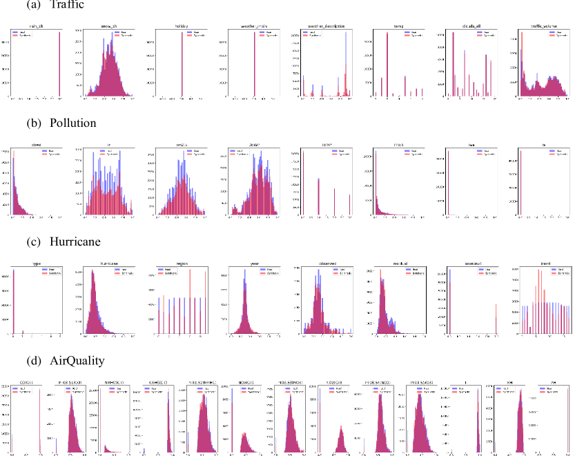
Figure 5: Plots of marginal distributions of real versus synthetic data: From top to bottom, Traffic, Pollution, Hurricane and AirQuality dataset.

Appendix G Visualization of entity conditional generation from C-TimeAutoDiff

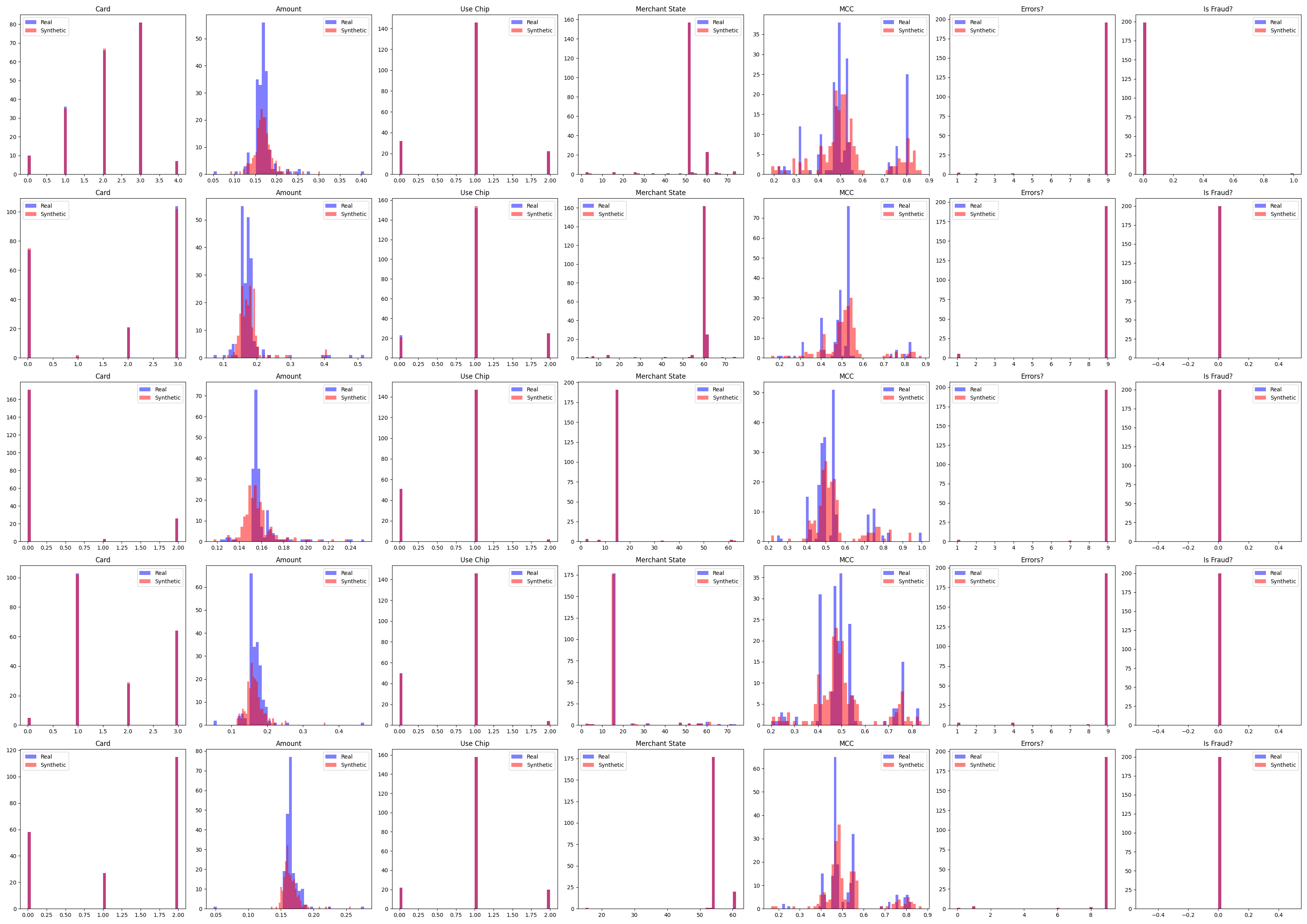
Figure 6: Plots of marginal distributions of real (card transaction) versus synthetic data: From top to bottom, sequential data of user number, 102, 614, 798, 1052, and 1800 in the original dataset, are generated, conditioned on labels of each 5 users.

Appendix H Computing resources

We ran the main model, TimeAutoDiff, on a computer equipped with an Intel(R) Core(TM) i7-8700 CPU @ 3.20GHz, 6 cores, 12 logical processors, an NVIDIA GeForce RTX 2080, and Intel(R) UHD Graphics 630. The training epochs for VAE and diffusion model were both set to be 50,000 over the entire datasets considered in this work.

Appendix I Broader societal impacts of TimeAutoDiff and safeguard guidance.

Positive Impacts: TimeAutoDiff has the potential to significantly impact society in several positive ways. By leveraging latent diffusion models to generate synthetic time series tabular data, it can accelerate research and innovation across scientific and engineering domains, providing high-fidelity data for experiments and hypothesis validation without the need for costly real-world data collection. This can be particularly beneficial in fields such as climate science, finance, healthcare, and engineering. The model can enhance the training of AI and machine learning models by providing diverse and representative datasets, leading to more robust and generalizable models. Furthermore, it can reduce costs associated with data collection and processing, enabling more cost-effective operations and aiding strategic planning and decision-making. In educational settings, TimeAutoDiff can provide students and educators with access to rich, diverse datasets, enhancing the learning experience in data science and machine learning courses. By facilitating the generation of balanced and unbiased synthetic datasets, it can contribute to the development of fair and ethical AI systems. Additionally, its ability to simulate various disaster scenarios can enhance preparedness and resilience in emergency and disaster management.

Negative Impacts: The widespread use of TimeAutoDiff also presents potential negative societal impacts. The ability to generate high-fidelity synthetic data can be misused for creating deceptive or fraudulent information, leading to ethical and legal concerns. Over-reliance on synthetic data might result in neglecting the importance of real-world data collection, potentially leading to biased or incomplete analyses. Despite significant improvements, synthetic data may still lack the quality and reliability of real-world data, which can impact decision-making processes in critical areas like healthcare and finance. Widespread use of synthetic data can also lead to skepticism and mistrust among stakeholders, undermining confidence in research findings and AI models. Additionally, generating high-quality synthetic data using advanced models like TimeAutoDiff can be computationally intensive, requiring significant resources that may not be accessible to all organizations, potentially widening the gap between resource-rich and resource-poor entities. It is also important to note that TimeAutoDiff has not been studied under privacy metrics, which means its effectiveness in preserving data privacy is uncertain. Finally, the use of synthetic data in modeling and decision-making might lead to unforeseen consequences, with models trained on synthetic data behaving unpredictably when exposed to real-world scenarios not captured in the synthetic data. Balancing these impacts is crucial for ensuring that the deployment of such models contributes positively to societal well-being and development.

Safeguard Guidance: To ensure the responsible use of TimeAutoDiff, implement safeguards such as establishing clear ethical guidelines, integrating privacy-preserving techniques like differential privacy, and ensuring robust data quality checks. Maintain transparency in the data generation process, conduct regular audits and assessments, and provide training for users on responsible use. Limit access to synthetic data to authorized personnel, engage with ethics and data science experts, and perform scenario testing to identify potential biases or unintended consequences. Adopt an incremental deployment strategy to identify and address issues in a controlled environment before widespread adoption.

References

- [1] Marin Biloš, Kashif Rasul, Anderson Schneider, Yuriy Nevmyvaka, and Stephan Günnemann. Modeling temporal data as continuous functions with stochastic process diffusion. 2023.
- [2] Yinan Cheng, Chi-Hua Wang, Vamsi K Potluru, Tucker Balch, and Guang Cheng. Downstream task-oriented generative model selections on synthetic data training for fraud detection models. arXiv preprint arXiv:2401.00974, 2024.
- [3] Ashkan Farhangi, Jiang Bian, Arthur Huang, Haoyi Xiong, Jun Wang, and Zhishan Guo. Aa-forecast: anomaly-aware forecast for extreme events. Data Mining and Knowledge Discovery, 37(3):1209–1229, March 2023.
- [4] Ian Goodfellow, Jean Pouget-Abadie, Mehdi Mirza, Bing Xu, David Warde-Farley, Sherjil Ozair, Aaron Courville, and Yoshua Bengio. Generative adversarial networks. Communications of the ACM, 63(11):139–144, 2020.
- [5] Irina Higgins, Loic Matthey, Arka Pal, Christopher Burgess, Xavier Glorot, Matthew Botvinick, Shakir Mohamed, and Alexander Lerchner. beta-vae: Learning basic visual concepts with a constrained variational framework. In International conference on learning representations, 2016.
- [6] Irina Higgins, Loic Matthey, Arka Pal, Christopher P Burgess, Xavier Glorot, Matthew M Botvinick, Shakir Mohamed, and Alexander Lerchner. beta-vae: Learning basic visual concepts with a constrained variational framework. ICLR (Poster), 3, 2017.
- [7] Jonathan Ho, Ajay Jain, and Pieter Abbeel. Denoising diffusion probabilistic models. Advances in neural information processing systems, 33:6840–6851, 2020.
- [8] Jonathan Ho and Tim Salimans. Classifier-free diffusion guidance. arXiv preprint arXiv:2207.12598, 2022.
- [9] Sepp Hochreiter and Jürgen Schmidhuber. Long short-term memory. Neural computation, 9(8):1735–1780, 1997.
- [10] Emiel Hoogeboom, Vıctor Garcia Satorras, Clément Vignac, and Max Welling. Equivariant diffusion for molecule generation in 3d. In International Conference on Machine Learning, pages 8867–8887. PMLR, 2022.
- [11] Din-Yin Hsieh, Chi-Hua Wang, and Guang Cheng. Improve fidelity and utility of synthetic credit card transaction time series from data-centric perspective. arXiv preprint arXiv:2401.00965, 2024.
- [12] Xin Huang, Ashish Khetan, Milan Cvitkovic, and Zohar Karnin. Tabtransformer: Tabular data modeling using contextual embeddings. arXiv preprint arXiv:2012.06678, 2020.
- [13] Jayoung Kim, Chaejeong Lee, and Noseong Park. Stasy: Score-based tabular data synthesis. arXiv preprint arXiv:2210.04018, 2022.
- [14] Diederik P Kingma and Max Welling. Auto-encoding variational bayes. arXiv preprint arXiv:1312.6114, 2013.
- [15] Akim Kotelnikov, Dmitry Baranchuk, Ivan Rubachev, and Artem Babenko. Tabddpm: Modelling tabular data with diffusion models. arXiv preprint arXiv:2209.15421, 2022.
- [16] Nicholas I Kuo, Louisa Jorm, Sebastiano Barbieri, et al. Synthetic health-related longitudinal data with mixed-type variables generated using diffusion models. arXiv preprint arXiv:2303.12281, 2023.
- [17] Chaejeong Lee, Jayoung Kim, and Noseong Park. Codi: Co-evolving contrastive diffusion models for mixed-type tabular synthesis. arXiv preprint arXiv:2304.12654, 2023.
- [18] Jin Li, Benjamin J Cairns, Jingsong Li, and Tingting Zhu. Generating synthetic mixed-type longitudinal electronic health records for artificial intelligent applications. NPJ Digital Medicine, 6(1):98, 2023.
- [19] Haksoo Lim, Minjung Kim, Sewon Park, Jaehoon Lee, and Noseong Park. Tsgm: Regular and irregular time-series generation using score-based generative models. Openreview, 2023.
- [20] Haksoo Lim, Minjung Kim, Sewon Park, and Noseong Park. Regular time-series generation using sgm. arXiv preprint arXiv:2301.08518, 2023.
- [21] Zinan Lin, Alankar Jain, Chen Wang, Giulia Fanti, and Vyas Sekar. Using gans for sharing networked time series data: Challenges, initial promise, and open questions. In Proceedings of the ACM Internet Measurement Conference, pages 464–483, 2020.
- [22] Xingchao Liu, Lemeng Wu, Mao Ye, et al. Learning diffusion bridges on constrained domains. In The Eleventh International Conference on Learning Representations, 2022.
- [23] Simone Luetto, Fabrizio Garuti, Enver Sangineto, Lorenzo Forni, and Rita Cucchiara. One transformer for all time series: Representing and training with time-dependent heterogeneous tabular data. arXiv preprint arXiv:2302.06375, 2023.
- [24] Yidong Ouyang, Liyan Xie, Chongxuan Li, and Guang Cheng. Missdiff: Training diffusion models on tabular data with missing values. arXiv preprint arXiv:2307.00467, 2023.
- [25] Inkit Padhi, Yair Schiff, Igor Melnyk, Mattia Rigotti, Youssef Mroueh, Pierre Dognin, Jerret Ross, Ravi Nair, and Erik Altman. Tabular transformers for modeling multivariate time series. In ICASSP 2021-2021 IEEE International Conference on Acoustics, Speech and Signal Processing (ICASSP), pages 3565–3569. IEEE, 2021.
- [26] Inkit Padhi, Yair Schiff, Igor Melnyk, Mattia Rigotti, Youssef Mroueh, Pierre Dognin, Jerret Ross, Ravi Nair, and Erik Altman. Tabular transformers for modeling multivariate time series. In ICASSP 2021 - 2021 IEEE International Conference on Acoustics, Speech and Signal Processing (ICASSP). IEEE, June 2021.
- [27] Nasim Rahaman, Aristide Baratin, Devansh Arpit, Felix Draxler, Min Lin, Fred Hamprecht, Yoshua Bengio, and Aaron Courville. On the spectral bias of neural networks. In International Conference on Machine Learning, pages 5301–5310. PMLR, 2019.
- [28] Robin Rombach, Andreas Blattmann, Dominik Lorenz, Patrick Esser, and Björn Ommer. High-resolution image synthesis with latent diffusion models. In Proceedings of the IEEE/CVF conference on computer vision and pattern recognition, pages 10684–10695, 2022.
- [29] Florian Schroff, Dmitry Kalenichenko, and James Philbin. Facenet: A unified embedding for face recognition and clustering. In Proceedings of the IEEE conference on computer vision and pattern recognition, pages 815–823, 2015.
- [30] Mike Schuster and Kuldip K Paliwal. Bidirectional recurrent neural networks. IEEE transactions on Signal Processing, 45(11):2673–2681, 1997.
- [31] Jascha Sohl-Dickstein, Eric Weiss, Niru Maheswaranathan, and Surya Ganguli. Deep unsupervised learning using nonequilibrium thermodynamics. In International conference on machine learning, pages 2256–2265. PMLR, 2015.
- [32] Yang Song, Jascha Sohl-Dickstein, Diederik P Kingma, Abhishek Kumar, Stefano Ermon, and Ben Poole. Score-based generative modeling through stochastic differential equations. arXiv preprint arXiv:2011.13456, 2020.
- [33] Mihaela Cătălina Stoian, Salijona Dyrmishi, Maxime Cordy, Thomas Lukasiewicz, and Eleonora Giunchiglia. How realistic is your synthetic data? constraining deep generative models for tabular data. arXiv preprint arXiv:2402.04823, 2024.
- [34] Namjoon Suh, Xiaofeng Lin, Din-Yin Hsieh, Merhdad Honarkhah, and Guang Cheng. Autodiff: combining auto-encoder and diffusion model for tabular data synthesizing. arXiv preprint arXiv:2310.15479, 2023.
- [35] Yusuke Tashiro, Jiaming Song, Yang Song, and Stefano Ermon. Csdi: Conditional score-based diffusion models for probabilistic time series imputation. Advances in Neural Information Processing Systems, 34:24804–24816, 2021.
- [36] Muhang Tian, Bernie Chen, Allan Guo, Shiyi Jiang, and Anru R Zhang. Fast and reliable generation of ehr time series via diffusion models. arXiv preprint arXiv:2310.15290, 2023.
- [37] Ashish Vaswani, Noam Shazeer, Niki Parmar, Jakob Uszkoreit, Llion Jones, Aidan N Gomez, Łukasz Kaiser, and Illia Polosukhin. Attention is all you need. Advances in neural information processing systems, 30, 2017.
- [38] Lei Xu, Maria Skoularidou, Alfredo Cuesta-Infante, and Kalyan Veeramachaneni. Modeling tabular data using conditional gan. Advances in Neural Information Processing Systems, 32, 2019.
- [39] Jinsung Yoon, Daniel Jarrett, and Mihaela Van der Schaar. Time-series generative adversarial networks. Advances in neural information processing systems, 32, 2019.
- [40] Jinsung Yoon, Michel Mizrahi, Nahid Farhady Ghalaty, Thomas Jarvinen, Ashwin S Ravi, Peter Brune, Fanyu Kong, Dave Anderson, George Lee, Arie Meir, et al. Ehr-safe: generating high-fidelity and privacy-preserving synthetic electronic health records. NPJ Digital Medicine, 6(1):141, 2023.
- [41] Xinyu Yuan and Yan Qiao. Diffusion-ts: Interpretable diffusion for general time series generation. In The Twelfth International Conference on Learning Representations, 2023.
- [42] Hengrui Zhang, Jiani Zhang, Balasubramaniam Srinivasan, Zhengyuan Shen, Xiao Qin, Christos Faloutsos, Huzefa Rangwala, and George Karypis. Mixed-type tabular data synthesis with score-based diffusion in latent space. arXiv preprint arXiv:2310.09656, 2023.
- [43] Kevin Zhang, Neha Patki, and Kalyan Veeramachaneni. Sequential models in the synthetic data vault. arXiv preprint arXiv:2207.14406, 2022.
- [44] Zilong Zhao, Aditya Kunar, Robert Birke, and Lydia Y Chen. Ctab-gan: Effective table data synthesizing. In Asian Conference on Machine Learning, pages 97–112. PMLR, 2021.
- [45] Zilong Zhao, Aditya Kunar, Robert Birke, and Lydia Y Chen. Ctab-gan+: Enhancing tabular data synthesis. arXiv preprint arXiv:2204.00401, 2022.
- [46] Chaoyi Zhu, Jiayi Tang, Hans Brouwer, Juan F Pérez, Marten van Dijk, and Lydia Y Chen. Quantifying and mitigating privacy risks for tabular generative models. arXiv preprint arXiv:2403.07842, 2024.