Shortcut to adiabaticity and holonomic transformation are the same thing

Abstract

A stable and fast path linking arbitrary pair of quantum states is commonly desired for the engineering protocols inspired by stimulated Raman adiabatic passage, such as shortcut to adiabaticity and holonomic transformation. It has immediate applications in quantum control and quantum computation and is fundamental about the exact solution of a time-dependent Schrödinger equation. We construct a universal control framework based on the system dynamics within an ancillary picture, in which the system Hamiltonian is diagonal so that no transition exists among the ancillary bases during the time evolution. Practically the desired evolution path can be obtained by the von Neumann equation for the parametric ancillary bases. We demonstrate that our control framework can be reduced to the nonadiabatic holonomic quantum transformation, the Lewis-Riesenfeld theory for invariant, and the counterdiabatic driving method under distinct scenarios and conditions. Also it can be used to achieve the cyclic transfer of system population that could be a hard or complex problem for the existing methods. For the state engineering over a finite-dimensional quantum system, our work can provide a full-rank nonadiabatic time-evolution operator.

I Introduction

Real-time state control Král et al. (2007) over the quantum systems, such as holonomic transformation Zanardi and Rasetti (1999) and coherent population transfer among discrete quantum states Bergmann et al. (1998), is fundamental and central to quantum information processing Gisin and Thew (2007); Kimble (2008) and quantum networks Kimble (2008). Holonomic transformation aims to manipulate the computational states or subspace for the desired geometric quantum computation. Coherent population transfer aims to transfer population among the discrete states. Intuitively they seem distinct, the current work however attempts to find a systematic approach for understanding how they can be carried out under the same theoretical framework.

Geometric phase Dong et al. (2021) is the core concept for geometric quantum gate, started from the Abelian case Berry (1984); Aharonov and Anandan (1987) in both adiabatic and nonadiabatic passage and extended to the non-Abelian case Wilczek and Zee (1984); Anandan (1988); Zanardi and Rasetti (1999); De Chiara and Palma (2003); Leek et al. (2007); Filipp et al. (2009) in the degenerate subspace. In holonomic transformation, geometric phase provides an extra degree of freedom for the manipulation of the computational states and exemplifies the holonomy through the parallel transport around closed cycles to preserve the geometrical information to be transported Cohen et al. (2019). The holonomic transformation is then fault-tolerant to the local noise during the cyclic evolution, by which the geometric phase can be accumulated by adiabatic Born and Fock (1928); Jones et al. (2000); Duan et al. (2001) or nonadiabatic driving Sjöqvist et al. (2012); Liu et al. (2019). With the adiabatic changing Hamiltonian, the system has no dynamical phase Berry (1984); Wilczek and Zee (1984) yet suffers from the decoherence due to the long exposure to the environment. In the nonadiabatic case, the dynamical phase can vanish at each moment by the parallel-transport condition Sjöqvist et al. (2012); alternatively, the accumulated dynamical phase can be periodically eliminated with the spin-echo technique Jones et al. (2000); Liu et al. (2019) or the pulse-shaping method Liu et al. (2019) in the evolution process. Parallel transport is sensitive to the systematic errors in the precise control of the experimental parameters Zheng et al. (2016); Jing et al. (2017) and it can be partially released by path optimization.

Based on the adiabatic theorem Claridge (2009); Vitanov et al. (2017), the coherent population transfer in the three-level system can be described by a pedagogical model about the stimulated Raman adiabatic passage (STIRAP) Vitanov et al. (2017), that is widely used in a variety of disciplines including atomic, molecular, and optical physics Pillet et al. (1993); Phillips (1998) and quantum information processing García-Ripoll and Cirac (2003); Daems and Guérin (2007). In comparison to the counterpart by resonant driving or Rabi oscillation, the state transfer by STIRAP is notably featured with (i) the immunity to the spontaneous emission from the intermediate state and (ii) the robustness against the perturbations of experimental parameters. To avoid the non-negligible decoherence due to the longtime evolution of the open system Jing et al. (2016), many techniques including the Lewis-Riesenfeld (LR) theory for invariant and the counterdiabatic driving are proposed that could be under the name of the shortcut to adiabaticity (STA) Chen et al. (2010a); Guéry-Odelin et al. (2019); Baksic et al. (2016); Li and Chen (2016); Chen et al. (2010b, 2011); Chen and Muga (2012); Qi and Jing (2022). In particular, the LR-invariant method Chen et al. (2011); Chen and Muga (2012); Guéry-Odelin et al. (2019); Qi and Jing (2022) is found to be suitable for the quantum systems with the $SU(2)$ dynamical symmetry, such as the two-level atom Chen et al. (2011), the $\Lambda-$type qutrit Chen et al. (2010b); Chen and Muga (2012), and the continuous-variable systems with quadratic interaction Hamiltonian Qi and Jing (2022). With the transitionless quantum driving algorithm Berry (2009), the counterdiabatic driving method is developed on the adiabatic path Chen et al. (2010a); Guéry-Odelin et al. (2019); Qi and Jing (2022) and the dressed-state bases Baksic et al. (2016); Li and Chen (2016). These protocols, however, are essentially of the reverse engineering Guéry-Odelin et al. (2019), involved with unnecessary complexities in understanding the motivation and constrained by various scenarios.

In a distinctive perspective of forward engineering, we here design a universal control framework for the system dynamics within an ancillary picture, in which the time-dependent system Hamiltonian could be fully or partially diagonalized. The solution of the von Neumann equation for the undetermined ancillary bases yields the transitionless path for either shortcut-to-adiabaticity or holonomic transformation. The time-dependent Schrödinger equation can be exactly solved if a full-rank nonadiabatic evolution operator can be constructed, which means all the ancillary bases satisfy the von Neumann equation. Our universal framework provides a prescription that works for any state-transfer protocols and simplifies the discussion about holonomic transformation, STIRAP, and STA. In addition to demystify these techniques for quantum control, we propose a protocol for cyclic population transfer in a three-level system of $\Lambda$-type and a four-level system. It could then tackle a hard problem for the existing methods.

The rest part of this paper is structured as follows. In Sec. II, we introduce a general theoretical framework for time-dependent Hamiltonian. Section III contributes to comparing our universal protocol for state-transfer and the popular protocols such as nonadiabatic holonomic transformation, the Lewis-Riesenfeld theory for invariant, and the counterdiabatic driving method. Using a three-level system, it delivers the main message of this paper: all these versatile approaches could be unified with no unnecessary confusion. In Sec. IV, we apply our universal protocol to the problem of cyclic population transfer, exemplified with a three-level system of $\Lambda$-type and a four-level system. The whole work is concluded in Sec. V.

II General framework

Consider a closed quantum system of $N$ dimensions driven by a time-dependant Hamiltonian $H(t)$. In principle, we can always have a completed and orthonormal set to span the whole Hilbert space of the system, in which every basis is a pure-state solution to the Schrödinger equation ($\hbar\equiv 1$):

$$i\frac{d|\psi_{m}(t)\rangle}{dt}=H(t)|\psi_{m}(t)\rangle.$$ (1)

$|\psi_{m}(0)\rangle$, $1\leq m\leq N$, represents the undetermined initial state. Alternatively, the system dynamics can be described in an instantaneous picture with the bases $|\mu_{k}(t)\rangle$, which are not necessarily related to the Hamiltonian as well as the Schrödinger equation. With unitary transformation, the solution picture $|\psi_{m}(t)\rangle$ and the ancillary picture $|\mu_{k}(t)\rangle$ can be connected as

$$|\psi_{m}(t)\rangle=\sum_{k=1}^{N}c_{mk}(t)|\mu_{k}(t)\rangle,$$ (2)

where $c_{mk}(t)$ is the element of an $N\times N$ transformation matrix $\mathcal{C}$ at the $m$th row and the $k$th column. Substituting Eq. (2) into Eq. (1), we have collectively $N^{2}$ differential equations for all the matrix elements, e.g.,

$$\frac{d}{dt}c_{mk}(t)=i\sum_{l=1}^{N}\left[\mathcal{G}_{kl}(t)-\mathcal{D}_{kl}(t)\right]c_{ml}(t),$$ (3)

where $\mathcal{G}_{kl}(t)\equiv i\langle\mu_{k}(t)|\dot{\mu}_{l}(t)\rangle$ and $\mathcal{D}_{kl}(t)\equiv\langle\mu_{k}(t)|H(t)|\mu_{l}(t)\rangle$ represent the geometric (not explicitly dependent on the system Hamiltonian) and dynamical (explicitly dependent on Hamiltonian) contributions to the proportional factor, respectively. It is however hard to directly solve Eq. (3) due to the fact that every $c_{mk}(t)$ is coupled to the other $N-1$ elements $c_{ml}(t)$, $1\leq l\neq k\leq N$.

To simplify Eq. (3), one can further consider the system Hamiltonian and the proportional factor in a time-independent picture $|\mu_{k}(0)\rangle$. With the unitary rotation by $V(t)\equiv\sum_{k=1}^{N}|\mu_{k}(t)\rangle\langle\mu_{k}(0)|$, we have

$$H_{\rm rot}(t) =V^{\dagger}(t)H(t)V(t)-iV^{\dagger}(t)\frac{d}{dt}V(t)$$ (4)

$$=-\sum_{k=1}^{N}\sum_{l=1}^{N}\left[\mathcal{G}_{kl}(t)-\mathcal{D}_{kl}(t)\right]|\mu_{k}(0)\rangle\langle\mu_{l}(0)|.$$

It indicates that if $H_{\rm rot}(t)$ is diagonal for certain $k$’s, then the proportional factor $\mathcal{G}_{kl}(t)-\mathcal{D}_{kl}(t)$ becomes vanishing for $l\neq k$ and vice versa. Note this diagonalization could be full or partial as long as $\{k\}\in\{1,2,\cdots,N\}$. And when $\{k\}=\{1,2,\cdots,N\}$, $H_{\rm rot}(t)$ is fully diagonalized. In either case, Eq. (3) for certain $k$’s can be reduced to

$$\frac{d}{dt}c_{mk}(t)=i\left[\mathcal{G}_{kk}(t)-\mathcal{D}_{kk}(t)\right]c_{mk}(t).$$ (5)

It leads straightforwardly to the solution

$$c_{mk}(t) =e^{if_{k}(t)}c_{mk}(0)$$ (6)

$$f_{k}(t) \equiv\int_{0}^{t}\left[\mathcal{G}_{kk}(t^{\prime})-\mathcal{D}_{kk}(t^{\prime})\right]dt^{\prime}.$$

The diagonalization also suggests that the initial condition for certain ancillary base $|\mu_{k}(0)\rangle$ is under the constraint of the system Hamiltonian.

Main result.—Here we prove that the von Neumann equation for the ancillary projection operator $\Pi_{k}(t)\equiv|\mu_{k}(t)\rangle\langle\mu_{k}(t)|$, which reads

$$\frac{d}{dt}\Pi_{k}(t)=-i\left[H(t),\Pi_{k}(t)\right],$$ (7)

is a necessary and sufficient condition for the diagonalization of $H_{\rm rot}(t)$ in the bases $|\mu_{k}(0)\rangle$ with non-vanishing diagonal elements.

Necessary condition. When $H_{\rm rot}(t)$ is diagonal in the picture of $\{|\mu_{k}(0)\rangle\}$ and $\langle\mu_{k}(0)|H_{\rm rot}(t)|\mu_{k}(0)\rangle\neq 0$, equivalently we have a commutation expression as

$$\frac{d}{dt}\Pi_{k}(0)=-i\left[H_{\rm rot}(t),\Pi_{k}(0)\right]=0.$$ (8)

When the diagonalization is not full-rank, we can focus on the diagonalized subspace. Using the relation that $\Pi_{k}(0)=V^{\dagger}\Pi_{k}(t)V$ and Eq. (4), Eq. (8) can be written as

$$\frac{d\left[V^{\dagger}\Pi_{k}(t)V\right]}{dt}=-i\left[V^{\dagger}H(t)V-iV^{\dagger}\frac{d}{dt}V,V^{\dagger}\Pi_{k}(t)V\right].$$ (9)

By the chain rule, it becomes

$$V^{\dagger}\frac{d\Pi_{k}(t)}{dt}V =-i\left[V^{\dagger}H(t)V-iV^{\dagger}\frac{d}{dt}V,V^{\dagger}\Pi_{k}(t)V\right]$$ (10)

$$-\frac{dV^{\dagger}}{dt}\Pi_{k}(t)V-V^{\dagger}\Pi_{k}(t)\frac{dV}{dt}.$$

Multiplying Eq. (10) by $V(t)$ from left and by $V^{\dagger}(t)$ from right and using the complementary relation that $dV/dtV^{\dagger}=-VdV^{\dagger}/dt$, we have

$$\frac{d\Pi_{k}(t)}{dt} =-iV\left[V^{\dagger}H(t)V-iV^{\dagger}\frac{d}{dt}V,V^{\dagger}\Pi_{k}(t)V\right]V^{\dagger}$$ (11)

$$-V\frac{dV^{\dagger}}{dt}\Pi_{k}(t)-\Pi_{k}(t)\frac{dV}{dt}V^{\dagger}$$

$$=-i\left[H(t),\Pi_{k}(t)\right].$$

Thus the von Neumann equation (7) is a necessary condition for the diagonalization of $H_{\rm rot}(t)$ with nonvanishing elements $\langle\mu_{k}(0)|H_{\rm rot}(t)|\mu_{k}(0)\rangle$.

Sufficient condition. The von Neumann equation (7) is equivalent to

$$V^{\dagger}\frac{d\Pi_{k}(t)}{dt}V=-i\left[V^{\dagger}H(t)V,V^{\dagger}\Pi_{k}(t)V\right].$$ (12)

And by the chain rule, we have

$$\frac{d\left[V^{\dagger}\Pi_{k}(t)V\right]}{dt} =-i\left[V^{\dagger}H(t)V,V^{\dagger}\Pi_{k}(t)V\right]$$ (13)

$$+\frac{dV^{\dagger}}{dt}\Pi_{k}(t)V+V^{\dagger}\Pi_{k}(t)\frac{dV}{dt}$$

$$=-i\left[V^{\dagger}H(t)V-iV^{\dagger}\frac{dV}{dt},V^{\dagger}\Pi_{k}(t)V\right].$$

With rotation back to the time-independent picture, it returns to Eq. (8). Then we complete the proof of the sufficient condition for the diagonalization of $H_{\rm rot}(t)$ in the bases $|\mu_{k}(0)\rangle$. A close justification about the sufficient condition can be found in Ref. Liu et al. (2019), despite it focuses on merely a single path that could be solved by Eq. (5).

The most strong condition that all the ancillary bases $|\mu_{k}(t)\rangle$ with $1\leq k\leq N$ satisfy the von Neumann equation (7) indicates that $H_{\rm rot}(t)$ is diagonal in the whole Hilbert space. In another word, the diagonalized $H_{\rm rot}(t)$ in Eq. (4) is full-rank so that one can determine the exact solution for the time-dependent Schrödinger equation under $H(t)$ and the time-evolution operator reads,

$$U(t,0)=\sum_{k=1}^{N}e^{if_{k}(t)}|\mu_{k}(t)\rangle\langle\mu_{k}(0)|,$$ (14)

where $f_{k}(t)$ is the generated phase as defined in Eq. (6) for the ancillary basis $|\mu_{k}(t)\rangle$. The formulation of $U$ indicates that there exist no transitions among all the diagonalized bases, so that each of them can be used as an adiabatic path for (either accelerated or slow) state or population transfer. In a general case, $H_{\rm rot}(t)$ is diagonal with respective to $V(t)$ in a subspace spanned by $\tilde{N}$ ancillary bases, $\tilde{N}<N$, that satisfy Eq. (7). Then with proper initial states and reordering of ancillary bases, the system dynamics can be described by a reduced evolution operator, i.e., $\tilde{U}(t,0)=\sum_{k=1}^{\tilde{N}}e^{if_{k}(t)}|\mu_{k}(t)\rangle\langle\mu_{k}(0)|$.

The evolution operator formulated in Eq. (14) and its relieved version constitute the basic of holonomic transformation, STA, and STIRAP. For holonomic transformation, the phase factor $f_{k}(t)$ in Eqs. (6) or (14) can be used as an extra degree of freedom to manipulate the computational states. While for STA and STIRAP that bridge the initial and target states, $f_{k}(t)$ is not concerned with population transfer Guéry-Odelin et al. (2019). The existing control methods such as STA that are categorized to the reverse engineering determine the system Hamiltonian through the ansätz of a target evolution operator. In contrast, our control framework provides a forward-engineering perspective which diagonalizes the system Hamiltonian within the ancillary picture to obtain a possible outcome of evolution. The unitary transformation $V(t)$ is a quantum-mechanics counterpart to the point transformation that transforms the original coordinate to the generalized coordinate in analytical mechanics under constraint. And the possible evolution mimics the visual displacement.

III Our protocol versus existing control protocols

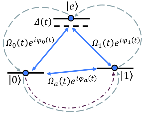
Figure 1: Sketch of a three-level system under control, in which the transitions $|0\rangle\leftrightarrow|e\rangle$ and $|1\rangle\leftrightarrow|e\rangle$ are driven by the fields of the same detuning and $|0\rangle\leftrightarrow|1\rangle$ is driven by a resonant driving field. The population transfer $|0\rangle\rightarrow|1\rangle$ and the cyclic population transfer $|0\rangle\rightarrow|1\rangle\rightarrow|e\rangle\rightarrow|0\rangle$ are described by the brown dot-dashed line and the gray dashed line, respectively.

In this section, we appreciate the utility and versatility of our framework by comparing with the well-known protocols for state control or population transfer Sjöqvist et al. (2012); Chen et al. (2010a); Chen and Muga (2012); Baksic et al. (2016); Liu et al. (2019). Through modifying the parametric setting, we demonstrate that our general framework can be reduced to the nonadiabatic holonomic transformation Sjöqvist et al. (2012); Liu et al. (2019), the LR invariant approach Chen and Muga (2012), and the counterdiabatic driving method Chen et al. (2010a); Baksic et al. (2016). As a pedagogical example, we here focus on transferring the population on $|0\rangle$ to $|1\rangle$ in a three-level system of $\Lambda$-type under control, which is marked by the brown dot-dashed line as shown in Fig. 1.

III.1 Our universal protocol for population transfer

Our protocol for population transfer in a three-level system (see Fig. 1) is based on three classical driving fields. In particular, the transitions $|0\rangle\leftrightarrow|e\rangle$ and $|1\rangle\leftrightarrow|e\rangle$ are respectively driven by the laser fields $\Omega_{0}(t)$ and $\Omega_{1}(t)$ with the same detuning $\Delta(t)$. $\varphi_{0}(t)$ and $\varphi_{1}(t)$ are two time-dependent phases. And the transition between the states $|0\rangle$ and $|1\rangle$ is driven by the resonant driving field with the Rabi frequency $\Omega_{a}(t)$ and the phase $\varphi_{a}(t)$. In experiments Koch et al. (2007); Vepsäläinen et al. (2019), the transition $|0\rangle\leftrightarrow|1\rangle$ of the superconducting transmon qubit can be achieved by a two-photon process Vepsäläinen et al. (2019). Then the full Hamiltonian in the original bases $\{|0\rangle,|1\rangle,|e\rangle\}$ reads

$$H(t) =\Delta(t)|e\rangle\langle e|+\Omega_{0}(t)e^{i\varphi_{0}(t)}|0\rangle\langle e|+\Omega_{1}(t)e^{i\varphi_{1}(t)}|1\rangle\langle e|$$ (15)

$$+\Omega_{a}(t)e^{i\varphi_{a}(t)}|0\rangle\langle 1|+{\rm H.c.}.$$

In general, we can describe the system dynamics in the ancillary picture spanned with the orthonormal time-dependant bases $\{|\mu_{0}(t)\rangle,|\mu_{1}(t)\rangle,|\mu_{2}(t)\rangle\}$, which read

$$|\mu_{0}(t)\rangle =\cos\theta(t)|0\rangle-\sin\theta(t)e^{-i\alpha(t)}|1\rangle,$$ (16)

$$|\mu_{1}(t)\rangle =\sin\theta(t)\sin\phi(t)|0\rangle+\cos\phi(t)e^{-i\beta(t)}|e\rangle$$

$$+\cos{\theta(t)}\sin\phi(t)e^{-i\alpha(t)}|1\rangle,$$

$$|\mu_{2}(t)\rangle =\sin\theta(t)\cos\phi(t)|0\rangle-\sin\phi(t)e^{-i\beta(t)}|e\rangle$$

$$+\cos\theta(t)\cos\phi(t)e^{-i\alpha(t)}|1\rangle,$$

where $\theta(t)$, $\phi(t)$, $\alpha(t)$ and $\beta(t)$ are time-dependant parameters. It is interesting to find that the Hamiltonian in the ancillary picture is full-rank, since every ancillary basis $|\mu_{k}(t)\rangle$ can satisfy the von Neumann equation (7) at the same time. Substituting Eq. (16) into Eq. (7), we find that the phases are

$$\varphi_{0}(t)-\varphi_{1}(t) =\alpha(t),$$ (17)

$$\varphi_{a}(t)-\alpha(t) =-\arctan\left[\frac{2\dot{\theta}(t)}{\dot{\alpha}(t)\tan 2\theta(t)}\right],$$

and the detuning and Rabi-frequencies are

$$\Delta(t) =2\Omega(t)\cot 2\phi(t)\cos\left[\varphi_{0}(t)-\beta(t)\right]$$ (18)

$$+\dot{\beta}(t)-\frac{1}{2}\dot{\alpha}(t)\tan 2\theta(t)\cot\theta(t),$$

$$\Omega_{0}(t) =\Omega(t)\sin\theta(t),$$

$$\Omega_{1}(t) =\Omega(t)\cos\theta(t),$$

$$\Omega_{a}(t) =\frac{\dot{\theta}(t)}{\sin\left[\varphi_{a}(t)-\alpha(t)\right]},$$

where $\Omega(t)\equiv\dot{\phi}(t)/\sin[\varphi_{0}(t)-\beta(t)]$. Each $|\mu_{k}(t)\rangle$ can be used as an accelerated adiabatic transfer path. $\theta(t)$ and $\phi(t)$ and their boundary conditions determine the specific evolution path from $|0\rangle$ to $|1\rangle$. In practice, the time dependence of $\theta(t)$ and $\phi(t)$ can be fully manipulated by the detuning and driving intensities. With no loss of generality, we can use the path $|\mu_{0}(t)\rangle$ in Eq. (16) by setting the boundary conditions $\theta(0)=k\pi$ and $\theta(T)=\pi/2+k\pi$ with integer $k$. $\phi(t)$ is found to be irrelevant in this task.

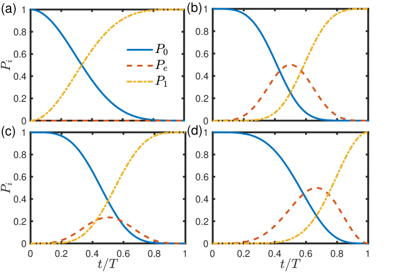
Figure 2: State populations $P_{i}$, $i=0,1,e$, versus the evolution time $t/T$ for (a) our control protocol, (b) the nonadiabatic holonomic transformation, (c) the Lewis-Riesenfeld theory for invariant, and (d) the counterdiabatic driving method in the dressed-state basis. The parameters are set according to (a) $\varphi_{i}(t)$, $i=0,1,a$, in Eq. (17) and $\Delta(t)$ and $\Omega_{i}(t)$ in Eq. (18) with $\varphi_{0}=\pi/2$, $\alpha=\beta=0$, $\theta(t)=\pi/2\sin(\pi t/2T)$, and $\phi(t)=\pi/2\cos(\pi t/2T)$, (b) $\Omega_{0}(t)$, $\Omega_{1}(t)$ and $\varphi_{0}(t)$ in Eq. (21) with $\phi(t)=\pi\cos(\pi t/T)$ and $\alpha(t)=2\pi\Theta(T/2)$ where $\Theta(t)$ is a step-function, (c) $\Omega_{0}(t)$ and $\Omega_{1}(t)$ in Eq. (25) with $\theta(t)=\pi t/2T$ and $\phi=0.2527$ Chen and Muga (2012), and (d) $\Omega_{0}(t)$ and $\Omega_{1}(t)$ in Eq. (29) with $\theta=\pi/4$ and $\phi(t)=\pi\cos(\pi t/2T)$.

The simulation results according to Eqs. (17) and (18) over the state populations $P_{i}=\langle i|\rho(t)|i\rangle$, $i=0,1,e$, are plotted in Fig. 2(a), where $\rho(t)$ is calculated by the time-dependent Schrödinger equation and $\rho(0)=|0\rangle\langle 0|$. In particular, the detuning $\Delta$ is set as zero by letting $\varphi_{0}=\pi/2$ and $\alpha=\beta=0$; and the Rabi frequencies are parameterized with $\theta(t)=\pi/2\sin(\pi t/2T)$ and $\phi(t)=\pi/2\cos(\pi t/2T)$. It is found that the population on the state $|0\rangle$ can be completely and smoothly transferred to the state $|1\rangle$ after a period $T$. Due to the formalization of the path $|\mu_{0}(t)\rangle$, there is no occupation on the undesired state $|e\rangle$ during the whole transfer process.

III.2 Nonadiabatic holonomic transformation

Our universal protocol for the three-level system can be reduced to the nonadiabatic holonomic transformation Sjöqvist et al. (2012); Liu et al. (2019) when the external driving between $|0\rangle\leftrightarrow|1\rangle$ in Fig. 1 is switched off, i.e., $\Omega_{a}=0$ and $\varphi_{a}=0$. And we set the detuning $\Delta(t)=0$ for simplicity. Thus the full Hamiltonian in Eq. (15) becomes

$$H(t)=\frac{\Omega_{0}(t)}{2}e^{i\varphi_{0}(t)}|0\rangle\langle e|+\frac{\Omega_{1}(t)}{2}e^{i\varphi_{1}(t)}|1\rangle\langle e|+{\rm H.c.},$$ (19)

where the time-dependant phases $\varphi_{0}(t)$ and $\varphi_{1}(t)$ contribute to the demanded geometric phase. In this case, the excited state $|e\rangle$ is regarded as an ancillary state and the lower states $|0\rangle$ and $|1\rangle$ constitute the computational subspace. In the dark-bright basis for the computational subspace, it turns out that relative to the dark state, a geometric phase is accumulated on the bright state, which could be used as an extra degree of freedom to determine the type of the quantum gate.

Practically, the ancillary picture can be spanned with the following orthonormal ancillary bases:

$$|\mu_{0}(t)\rangle =\cos\frac{\theta(t)}{2}|0\rangle+\sin\frac{\theta(t)}{2}e^{i\varphi(t)}|1\rangle,$$ (20)

$$|\mu_{1}(t)\rangle =\sin\frac{\phi(t)}{2}|b(t)\rangle+\cos\frac{\phi(t)}{2}e^{-i\alpha(t)}|e\rangle,$$

$$|\mu_{2}(t)\rangle =\cos\frac{\phi(t)}{2}|b(t)\rangle-\sin\frac{\phi(t)}{2}e^{-i\alpha(t)}|e\rangle,$$

where $|b(t)\rangle\equiv\sin\left[\theta(t)/2\right]|0\rangle-\cos\left[\theta(t)/2\right]e^{i\varphi(t)}|1\rangle$ is orthonormal to the ancillary base $|\mu_{0}(t)\rangle$, $\varphi(t)\equiv\varphi_{1}(t)-\varphi_{0}(t)$, and $\theta(t)$, $\phi(t)$ and $\alpha(t)$ are generally time dependent. Note Eq. (20) is a specific formation of the general case in Eq. (16) yet with the convention in Refs. Sjöqvist et al. (2012); Liu et al. (2019). Substituting $|\mu_{1}(t)\rangle$ and $|\mu_{2}(t)\rangle$ of Eq. (20) into the von Neumann equation (7), we have the Rabi-frequencies and the phase as

$$\Omega_{0}(t) =\Omega(t)\sin\frac{\theta(t)}{2},$$ (21)

$$\Omega_{1}(t) =-\Omega(t)\cos\frac{\theta(t)}{2},$$

$$\varphi_{0}(t) =\alpha(t)-\arctan\left[\frac{\dot{\phi}(t)}{\dot{\alpha}(t)\tan\phi(t)}\right],$$

where $\Omega(t)\equiv\dot{\phi}(t)/\sin[\varphi_{0}(t)-\alpha(t)]$. With Eq. (21), $|\mu_{0}(t)\rangle$ is found to be a dark state featured with zero eigenvalue and is decoupled from the system dynamics. The system dynamics are then constrained in the subspace $\{|\mu_{1}(t)\rangle,|\mu_{2}(t)\rangle\}$. And conventionally one considers a time-independent $\theta$ in the holonomic transformation.

Equation (14) indicates that if the system starts from the computational subspace and goes back to the same subspace through the path $|\mu_{1}(t)\rangle$ or $|\mu_{2}(t)\rangle$ (under respective boundary conditions), then a phase factor $f_{k}(t)$ can be generated on the bright state $|b(t)\rangle$ relative to the dark state $|\mu_{0}(t)\rangle$. The phase factor can be purely geometric when the dynamical part is eliminated.

In particular, if the system evolves along the path $|\mu_{1}(t)\rangle$, then by Eqs. (5) and (6) the phase factor can be expressed as $f_{1}(t)=\gamma_{g}(t)+\gamma_{d}(t)$, a summation of the geometric phase $\gamma_{g}(t)=\int_{0}^{t}\mathcal{G}_{11}(t^{\prime})dt^{\prime}$ with $\mathcal{G}_{11}(t)=\dot{\alpha}(t)\cos^{2}[\phi(t)/2]$ and the dynamical one $\gamma_{d}(t)=\int_{0}^{t}\mathcal{D}_{11}(t^{\prime})dt^{\prime}$ with $\mathcal{D}_{11}(t)=\Omega(t)\sin\phi(t)\cos[\varphi_{0}(t)-\alpha(t)]$. The dynamical phase $\gamma_{d}$ can remain zero when $\varphi_{0}(t)-\alpha(t)=\pi/2$, consistent with the parallel-transport condition Sjöqvist et al. (2012), or can vanish after a step-wise cancelation Jones et al. (2000); Liu et al. (2019). Under the parallel-transport condition, the geometric phase $\gamma_{g}$ can be simply obtained by setting $\alpha(t)$ or $\varphi_{0}(t)$ as a step function. For example, when $\alpha(t)=2\gamma\Theta(T/2)$ and $\phi(t)=\pi\cos(\pi t/T)$ (in regard of the boundary condition of the path $|\mu_{1}(t)\rangle$), the geometric phase is found to be $\gamma_{g}=\gamma$. Then the evolution operator for the holonomic transformation can be written as

$$U\left(\theta,\varphi(t),\gamma\right) =|\mu_{0}(t)\rangle\langle\mu_{0}(t)|-e^{i\gamma}|b(t)\rangle\langle b(t)|$$ (22)

$$=e^{i\gamma/2}e^{-i\gamma/2\vec{n}\cdot\vec{\sigma}},$$

where $\vec{n}\equiv(\sin\theta\cos\varphi(t),-\sin\theta\sin\varphi(t),\cos\theta)$ is the rotating axis. According to Eq. (21), $\theta$ is determined by the intensity ratio of the two driving fields; and according to Eq. (20), $\varphi(t)$ is their phase difference. The system population on the state $|0\rangle$ can be transferred to the state $|1\rangle$ by $U(\pi/2,0,\pi)$ according to Eq. (22). In Fig. 2(b), we plot the population dynamics for $|i\rangle$, $i=0,1,e$. It is found that the initial population on the state $|0\rangle$ can be completely transferred to the target state $|1\rangle$ in the end of the period. In contrast to Fig. 2(a) by our protocol, the ancillary state $|e\rangle$ can be temporarily occupied due to the formalization of $|\mu_{1}(t)\rangle$, e.g., $P_{e}=0.5$ when $t=T/2$. In addition to the population transformation, Eqs. (20) and (22) indicate that the phase $\gamma$ of the geometric gate can be manipulated by the phases of the computational states (ancillary bases).

III.3 Lewis-Riesenfeld theory for invariant

In the control field of shortcut-to-adiabaticity, the Lewis-Riesenfeld theory for invariant is popular to the systems following the $SU(2)$ dynamical symmetry, e.g., the two-level system Chen et al. (2011), the $\Lambda-$type qutrit Chen et al. (2010b); Chen and Muga (2012), and certain quadratic continuous-variable systems Qi and Jing (2022). In Fig. 1, when the driving between $|0\rangle$ and $|1\rangle$ is dropped and the other two driving fields are resonant and in phase, the Lewis-Riesenfeld theory for invariant Chen and Muga (2012) can emerge from our universal protocol. In this case, the full Hamiltonian in Eq. (15) can be reduced to

$$H(t)=\Omega_{0}(t)|0\rangle\langle e|+\Omega_{1}(t)|1\rangle\langle e|+{\rm H.c.}.$$ (23)

The system dynamics can be described within the ancillary picture with a complete set of orthogonal ancillary bases $\left\{|\mu_{0}(t)\rangle,|\mu_{1}(t)\rangle,|\mu_{2}(t)\rangle\right\}$ as

$$|\mu_{0}(t)\rangle =\sin{\theta(t)}|0\rangle-\cos{\theta(t)}|1\rangle,$$ (24)

$$|\mu_{1}(t)\rangle =\cos{\theta(t)}\sin{\phi(t)}|0\rangle+i\cos{\phi(t)}|e\rangle$$

$$+\sin{\theta(t)}\sin{\phi(t)}|1\rangle,$$

$$|\mu_{2}(t)\rangle =\cos{\theta(t)}\cos{\phi(t)}|0\rangle-i\sin{\phi(t)}|e\rangle$$

$$+\sin{\theta(t)}\cos{\phi(t)}|1\rangle$$

with the time-dependent parameters $\theta(t)$ and $\phi(t)$. The specific ancillary bases in Eq. (24) can be formulated by the general bases in Eq. (16) when $\theta(t)\rightarrow\pi/2-\theta$, $\alpha(t)=0$, and $\beta(t)=-\pi/2$. Instead of demonstrating the system dynamics within the whole Hilbert space, one can focus merely on the one-dimensional ancillary subspace consisting of the ancillary base $|\mu_{1}(t)\rangle$ or $|\mu_{2}(t)\rangle$, which is a superposed state of $|0\rangle$, $|1\rangle$, and $|e\rangle$. In another word, $H_{\rm rot}(t)$ of the situation in Eq. (23) can be partially diagonal in the ancillary bases as long as $|\mu_{1}(t)\rangle$ or $|\mu_{2}(t)\rangle$ satisfies the von Neumann equation (7). With $|\mu_{2}(t)\rangle$, the Rabi-frequencies $\Omega_{0}(t)$ and $\Omega_{1}(t)$ are found to be determined by

$$\Omega_{0}(t) =\dot{\theta}(t)\sin\theta(t)\cot\phi(t)+\dot{\phi}(t)\cos\theta(t),$$ (25)

$$\Omega_{1}(t) =-\dot{\theta}(t)\cos\theta(t)\cot\phi(t)+\dot{\phi}(t)\sin\theta(t),$$

that take the same formation in Ref. Chen and Muga (2012). Using Eq. (14), the relevant time-evolution operator can be written as

$$U(t,0)=e^{if_{2}(t)}|\mu_{2}(t)\rangle\langle\mu_{2}(0)|,$$ (26)

where $f_{2}(t)$ is the Lewis-Riesenfeld phase Guéry-Odelin et al. (2019) and it is not relevant to the population transfer.

Using Eq. (25) with $\theta(t)=\pi t/2T$ and $\phi=0.2527$ Chen and Muga (2012), we demonstrate in Fig. 2(c) the time evolution of populations $P_{i}$, $i=0,1,e$, by the Schrödinger equation. The three-level system is initially prepared as $|0\rangle$. The system population can be completely transferred to $|1\rangle$ after a period $T$. Yet during this evolution process, the mediated state $|e\rangle$ can be temporally populated due to the formalism of $|\mu_{0}(t)\rangle$. $P_{e}$ is as high as $P_{e}=0.22$ when $t=T/2$.

III.4 Counterdiabatic driving method in dressed-state basis

When the driving field on $|0\rangle\leftrightarrow|1\rangle$ of the three-level system in Fig. 1 is switched off, the driving fields on $|0\rangle\leftrightarrow|e\rangle$ and $|1\rangle\leftrightarrow|e\rangle$ are resonant in frequency, and their phases are time-independent, our control protocol can recover the counterdiabatic driving method in the dressed-state basis Baksic et al. (2016). Correspondingly, the Hamiltonian in Eq. (15) can be written as

$$H(t)=\Omega_{0}(t)e^{i\varphi_{0}}|0\rangle\langle e|+\Omega_{1}(t)e^{i\varphi_{1}}|1\rangle\langle e|+{\rm H.c.}.$$ (27)

And the ancillary picture can be spanned by those in Eq. (16) with $\alpha=\beta=0$. Using the components in this ancillary picture, the von Neumann equation (7) yields

$$\varphi_{0}=\varphi_{1}=\frac{\pi}{2},$$ (28)

$$\theta(t)\rightarrow\theta,$$

and

$$\Omega_{0}(t) =\Omega(t)\sin\theta,$$ (29)

$$\Omega_{1}(t) =\Omega(t)\cos\theta,$$

where $\Omega(t)\equiv\dot{\phi}(t)$. Under the conditions in Eqs. (28) and (29), $|\mu_{0}\rangle$ is time-independent and decoupled from the system dynamics. It is found that Eq. (29) can be either recovered by Eq. (21) for the nonadiabatic holonomic transformation when $\varphi_{0}-\alpha=\pi/2$, or by Eq. (25) for the Lewis-Riesenfeld theory when $\theta(t)$ is time independent. It can be expected since these three protocols stem from a similar evolution path.

With no loss of generality, one can suppose that the system evolves along the path $|\mu_{2}(t)\rangle$. Using Eq. (29) with $\theta=\pi/4$ and $\phi(t)=\pi\cos(\pi t/2T)$, the population dynamics of three levels $P_{i}$ are demonstrated in Fig. 2(d). It is found although the initial population on the state $|0\rangle$ can be fully transferred to the state $|1\rangle$ after a period $T$. The mediated state $|e\rangle$ can be significantly populated. When $t=0.65T$, $P_{e}=0.5$. Distinct from Figs. 2(a), (b), and (c), the whole pattern is asymmetrical to $t=T/2$.

III.5 Counterdiabatic driving with ancillary Hamiltonian

When the detuning $\Delta$ of the driving fields on the transitions $|0\rangle\leftrightarrow|e\rangle$ and $|1\rangle\leftrightarrow|e\rangle$ of the three-level system in Fig. 1 and the phases $\varphi_{0}$, $\varphi_{1}$ and $\varphi_{a}$ are time-independent, our universal protocol can simulate the counterdiabatic driving method via adiabatic passage Chen et al. (2010a). In the language of quantum transitionless driving Berry (2009), the whole Hamiltonian in Eq. (15) can be decomposed into the reference Hamiltonian $H_{0}(t)$ and the ancillary Hamiltonian $H_{c}(t)$ as

$$H(t)=H_{0}(t)+H_{c}(t),$$ (30)

where

$$H_{0}(t) =\Delta|e\rangle\langle e|+\Omega_{0}(t)e^{i\varphi_{0}}|0\rangle\langle e|+\Omega_{1}(t)e^{i\varphi_{1}}|1\rangle\langle e|,$$ (31)

$$H_{c}(t) =\Omega_{a}(t)e^{i\varphi_{a}}|0\rangle\langle 1|+{\rm H.c.}.$$

The basic idea of the counterdiabatic driving method is that the system can follow one instantaneous eigenstate of $H_{0}(t)$ with the assistance of $H_{c}(t)$. We demonstrate that the transitionless driving algorithm Berry (2009) can be described within the ancillary picture spanned by the ancillary bases $|\mu_{k}(t)\rangle$, $k=0,1,2$, in Eq. (16) with $\alpha=\beta=0$. In this ancillary picture, the von Neumann equation (7) yields

$$\varphi_{a}=\frac{\pi}{2},\quad\varphi_{0}=\varphi_{1}=0,$$ (32)

and the detuning and the Rabi-frequencies are

$$\Delta=2\Omega(t)\cot 2\phi(t),$$ (33)

$$\Omega_{0}(t)=\Omega(t)\sin\theta(t),$$

$$\Omega_{1}(t)=\Omega(t)\cos\theta(t),$$

$$\Omega_{a}(t)=\dot{\theta}(t),$$

where $\Omega(t)$ can be regarded as a field intensity for normalization.

We consider the case with a fixed $\phi$, which means $\Omega$ is also a constant. In this case, Eq. (33) recovers the formalization of counterdiabatic driving method for the adiabatic passage in Ref. Chen et al. (2010a). Along the same evolution path $|\mu_{0}(t)\rangle$, our universal protocol yields the same results about the populations $P_{i}$, $i=0,1,e$, as those in Ref. Chen et al. (2010a). They can be exactly described by Fig. 2(a). When the time-dependence of $\phi$ is relieved, $\phi\rightarrow\phi(t)$, our protocol can be used to transfer the system population to the state $|e\rangle$ by using $|\mu_{1}(t)\rangle$ or $|\mu_{2}(t)\rangle$. In another word, the application range of the counterdiabatic driving method can be straightforwardly extended in our universal framework.

IV Cyclic population transfer

More than unifying the existing protocols on quantum state engineering Sjöqvist et al. (2012); Chen et al. (2010a); Chen and Muga (2012); Baksic et al. (2016); Liu et al. (2019), our protocol in Sec. II is sufficiently universal to go readily beyond their reach. This section exemplifies the cyclic population transfers among three states in the three-level system (see the gray dashed lines in Fig. 1) and in the four-level system (see Fig. 5), which demonstrate the control power of our protocol in the unidirectional state transfer.

IV.1 Three-level system

Continuous cyclic population transfer among all the three levels $|0\rangle$, $|e\rangle$, and $|1\rangle$ could be a repetition of a single-loop of $|0\rangle\rightarrow|e\rangle\rightarrow|1\rangle\rightarrow|0\rangle$ with every loop starting from the state that all the populations are at $|0\rangle$. We can divide such a single loop into two stages.

On Stage $1$, one can employ the (accelerated) adiabatic path

$$|\mu_{2}(t)\rangle =\sin\theta(t)\cos\phi(t)|0\rangle-\sin\phi(t)e^{-i\beta(t)}|e\rangle$$ (34)

$$+\cos\theta(t)\cos\phi(t)e^{-i\alpha(t)}|1\rangle,$$

in Eq. (16). It is an ansätz for one of the ancillary bases having $|e\rangle$. The three ancillary bases span a time-dependent picture for the system with a general Hamiltonian in Eq. (15). Conditions for the driving phases, detuning, and intensities in Eqs. (17) and (18) can ensure that there exists no transition among the ancillary bases during the whole transfer process, as a result from the von Neumann equation (7). In particular, we could set $|\mu_{2}(t)\rangle$ as

$$\theta(t)=\frac{\pi}{2}\cos\left(\frac{\pi t}{2T}\right),\quad\phi(t)=\frac{\pi}{2}\sin\left(\frac{\pi t}{T}\right).$$ (35)

Then the population is transferred from $|0\rangle$ to $|e\rangle$ at $t=T/2$ and then transferred to $|1\rangle$ at $t=T$.

On Stage $2$, one can employ the path

$$|\mu_{0}(t)\rangle=\cos\theta(t)|0\rangle-\sin\theta(t)e^{-i\alpha(t)}|1\rangle$$ (36)

in Eq. (16) to move the system population back to $|0\rangle$. In particular, we set

$$\theta(t)=\frac{\pi}{2}\cos\left(\frac{\pi t}{T}\right),\quad\phi(t)=\frac{\pi}{2}\sin\left(\frac{2\pi t}{T}\right).$$ (37)

for the boundary conditions of the path $|\mu_{0}(t)\rangle$. This stage lasts $T/2$, then the first loop is completed.

In general, the $k$th loop of cyclic population transfer during $t\in[3(k-1)T/2,3kT/2]$, $k\geq 1$, can be divided into two stages. For Stage $1$, the parameters of $|\mu_{2}(t)\rangle$ can be set as

$$\theta(t) =\frac{\pi}{2}\sin\left[\frac{\pi(2t-(3k-1)T)}{4T}\right],$$ (38)

$$\phi(t) =-\frac{\pi}{2}\cos\left[\frac{\pi(2t-3kT)}{2T}\right],$$

then the population on $|0\rangle$ is transferred to $|e\rangle$ at $t=(3k-2)T/2$, and transferred to $|1\rangle$ at $t=(3k-1)T/2$. For Stage $2$ via the path $|\mu_{0}(t)\rangle$, we have

$$\theta(t) =-\frac{\pi}{2}\sin\left[\frac{\pi(2t-3kT)}{2T}\right],$$ (39)

$$\phi(t) =-\frac{\pi}{2}\sin\left[\frac{\pi(2t-3kT)}{T}\right],$$

which transfers the population on $|1\rangle$ back to $|0\rangle$ at $t=3kT/2$.

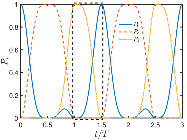
Figure 3: State populations $P_{i}$, $i=0,1,e$, versus the evolution time $t/T$ during the cyclic population transfer. The transfer process via the path $|\mu_{0}(t)\rangle$ in the first loop is marked with a black dashed-line frame. The phases $\varphi_{i}(t)$, $i=0,1,a$, are set according to Eq. (17) with $\alpha=0$ and $\varphi_{0}=\pi/2$. The Rabi-frequencies $\Omega_{i}(t)$ are set according to Eq. (18) with $\beta=0$, $\theta(t)$ and $\phi(t)$ in Eqs. (35), (37), (38), and (39).

Using Eqs. (17) and (18) with $\alpha=\beta=0$ and $\theta(t)$ and $\phi(t)$ given in Eqs. (35), (37), (38), and (39), we demonstrate in Fig. 3 the population dynamics of three levels $P_{i}$ for the cyclic transfer. It is shown that every loop of $|0\rangle\rightarrow|e\rangle\rightarrow|1\rangle\rightarrow|0\rangle$ is completed in a period of $3T/2$. The population transfers from $|0\rangle$ to $|e\rangle$ during $t\in[0,T/2]$ and from $|1\rangle$ to $|0\rangle$ during $t\in[T,3T/2]$ are faithful since the respectively unwanted states $|1\rangle$ and $|e\rangle$ are hardly populated. In contrast, during the transfer from $|e\rangle$ to $|1\rangle$, i.e., $t\in[T/2,T]$, the state $|0\rangle$ could be slightly populated, e.g., $P_{0}=0.08$ when $t=0.82T$. Yet it does not obstruct the complete transfer $P_{1}=1$ when $t=T$. In addition, the transfer process during $t\in[T,3T/2]$, which is distinguished with the black dashed-line frame in Fig. 3, is a typical evolution observed in STIRAP Král et al. (2007); Vitanov et al. (2017) and counterdiabatic driving Chen et al. (2010a). This process does not involve with the intermediate state $|e\rangle$ due to the formalization of the popular path $|\mu_{0}(t)\rangle$.

More generally, the population on any initial state can be transferred to an arbitrary target state via any ancillary base when it is permitted by the boundary condition. Alternatively, the loop of cyclic transfer can be $|0\rangle\rightarrow|1\rangle\rightarrow|e\rangle\rightarrow|0\rangle$. For example, along the path $|\mu_{0}(t)\rangle$ with $\alpha=0$, $\theta(0)=0$, $\phi(0)\rightarrow\phi$, $\theta(T/2)=\pi/2$, and $\phi(T/2)=\pi/2$, the system population can be firstly transferred from $|0\rangle$ to $|1\rangle$. Next, it can be transferred as $|1\rangle\rightarrow|e\rangle\rightarrow|0\rangle$ via the path $|\mu_{2}(t)\rangle$ with $\beta=0$, $\theta(T/2)=\phi(T/2)=0$, $\theta(T)\rightarrow\theta$, $\phi(T)=\pi/2$, $\theta(3T/2)=\pi/2$, and $\phi(3T/2)=0$.

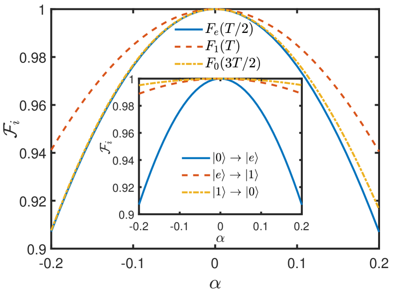
Figure 4: Fidelity of the state transfer as a function of the local dimensionless error $\alpha$ in the Rabi-frequency $\Omega_{0}(t)$ for the driving between $|0\rangle$ and $|e\rangle$. The other parameters are set the same as Fig. 3.

Within our universal protocol for the three-level system, the cyclic loop of population transfer in either direction requires a full-rank nonadiabatic evolution operator. It is based on the manipulation over $3$ degrees of freedom of the system, i.e., the Rabi-frequencies of the three driving fields. In contrast, the counterdiabatic driving method Chen et al. (2010a) had to employ the Rabi-frequencies of $5$ driving fields to achieve a full-rank evolution. As compared to the configuration in Fig. 1, $2$ more degrees of freedom are provided by two extra driving fields on the transitions $|0\rangle\leftrightarrow|e\rangle$ and $|1\rangle\leftrightarrow|e\rangle$, respectively. Then our universal protocol offers a resource-saving technique for the demonstration of full-rank nonadiabatic evolution.

To test the robustness of the evolution path against the fluctuation of experimental parameters, we consider a situation that allows the driving intensity $\Omega_{0}(t)$ between $|0\rangle$ and $|e\rangle$ to deviate from the setting in Eq. (18). The error influences both stages represented by Eqs. (34) and (36) in the cyclic loops. In particular, there exists a local dimensionless error $\alpha$ in the driving intensity, $\Omega_{0}(t)\rightarrow(1+\alpha)\Omega_{0}(t)$. The performance of the practical evolution path can be evaluated by the state fidelity $F_{i}=\langle i|\rho(t)|i\rangle$, where $|i\rangle$, $i=0,1,e$, is a varying target state in the cyclic loop. In Fig. 4, we demonstrate $F_{i}$ as a function of $\alpha$ at the desired time points $t=T/2,T,3T/2$ for the population transfer. In the main frame, the error presents in the whole process and in the sub-frame, it presents only in the specified period. It is found that the fidelity is more sensitive during the process $|0\rangle\rightarrow|e\rangle$ than the other two. The fidelity generally decreases with the error magnitude. Yet even when $|\alpha|=0.2$, $F_{e}$ is still above $0.91$.

IV.2 Four-level system

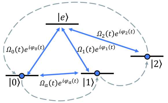
Figure 5: Sketch of a four-level system, in which the transitions $|e\rangle\leftrightarrow|i\rangle$, $i=0,1,2$, and $|0\rangle\leftrightarrow|1\rangle$ are driven by the resonant driving fields. The cyclic population transfer $|2\rangle\rightarrow|0\rangle\rightarrow|1\rangle\rightarrow|2\rangle$ is marked by the gray dashed line.

In this section, we consider a four-level system under four resonant driving fields with Rabi frequencies $\Omega_{i}(t)$ and phases $\varphi_{i}(t)$, $i=0,1,2,a$. It is not the most general configuration since our target is to realize the cyclic transfer among $|0\rangle$, $|1\rangle$, and $|2\rangle$ as indicated in Fig. 5, the same as Sec. IV.1. The Hamiltonian can be written as

$$H(t)=\Omega_{0}(t)e^{i\varphi_{0}(t)}|0\rangle\langle e|+\Omega_{1}(t)e^{i\varphi_{1}(t)}|1\rangle\langle e|$$ (40)

$$+\Omega_{2}(t)e^{i\varphi_{2}(t)}|2\rangle\langle e|+\Omega_{a}(t)e^{i\varphi_{a}(t)}|0\rangle\langle 1|+{\rm H.c.}.$$

By extending the three-dimensional case in Eq. (16) or its specific form in Eq. (24), a four-dimensional ancillary basis could be constructed as

$$|\mu_{0}(t)\rangle =\cos\theta(t)|0\rangle-\sin\theta(t)|1\rangle,$$ (41)

$$|\mu_{1}(t)\rangle =\sin\phi(t)\sin\theta(t)|0\rangle+\cos\phi(t)|e\rangle$$

$$+\sin\phi(t)\cos\theta(t)|1\rangle,$$

$$|\mu_{2}(t)\rangle =\cos\chi(t)\cos\phi(t)\sin\theta(t)|0\rangle-\cos\chi(t)\sin\phi(t)|e\rangle$$

$$+\cos\chi(t)\cos\phi(t)\cos\theta(t)|1\rangle+\sin\chi(t)|2\rangle,$$

$$|\mu_{3}(t)\rangle =\sin\chi(t)\cos\phi(t)\sin\theta(t)|0\rangle-\sin\chi(t)\sin\phi(t)|e\rangle$$

$$+\sin\chi(t)\cos\phi(t)\cos\theta(t)|1\rangle-\cos\chi(t)|2\rangle,$$

where $\chi(t)$, $\phi(t)$, and $\theta(t)$ are time-dependant parameters. Due to the lack of a sufficient number of degrees of freedom, i.e., the absence of the driving fields on the transitions $|0\rangle\leftrightarrow|2\rangle$ and $|1\rangle\leftrightarrow|2\rangle$, only two of the four ancillary bases can satisfy the von Neumann equation (7) at the same time. Thus if $|\mu_{0}(t)\rangle$ and $|\mu_{2}(t)\rangle$ are selected to span a two-dimensional subspace for the controllable dynamics, then one can construct the cyclic population transfer along the repeated loop $|2\rangle\rightarrow|0\rangle\rightarrow|1\rangle\rightarrow|2\rangle$. In particular, the von Neumann equation (7) for $|\mu_{0}(t)\rangle$ and $|\mu_{2}(t)\rangle$ gives rise to the phases as

$$\varphi_{0}=\varphi_{1}=\varphi_{a}=\frac{\pi}{2},\quad\varphi_{2}=-\frac{\pi}{2},$$ (42)

and the Rabi-frequencies as

$$\Omega_{0}(t)=\Omega(t)\sin\theta(t),$$ (43)

$$\Omega_{1}(t)=\Omega(t)\cos\theta(t),$$

$$\Omega_{2}(t)=\frac{\dot{\chi}(t)}{\sin\phi(t)},$$

$$\Omega_{a}(t)=\dot{\theta}(t),$$

where $\Omega(t)=\dot{\chi}(t)\tan\chi(t)\cot\phi(t)+\dot{\phi}(t)$. These two equations ensure that there is no transition between $|\mu_{0}(t)\rangle$ and $|\mu_{2}(t)\rangle$ during the whole evolution process. In addition, a nonzero $\Omega(t)$, the formation of $|\mu_{0}(t)\rangle$ and $|\mu_{2}(t)\rangle$, and their boundary conditions for cyclic transfer determine that $|e\rangle$ can not be fully populated.

With no loss of generality, the initial state that all the populations are at $|2\rangle$ could be cyclically transferred as $|2\rangle\rightarrow|0\rangle\rightarrow|1\rangle\rightarrow|2\rangle$. The whole transfer process can be divided into three stages. On Stage $1$, the system follows the path $|\mu_{2}(t)\rangle$ in Eq. (41) and the boundary conditions could be set as

$$\phi(t) =\frac{\pi}{2}\cos\frac{\pi t}{T},$$ (44)

$$\chi(t) =\frac{\pi}{2}\left[\cos\phi(t)-1\right],$$

$$\theta(t) =-\frac{\pi}{2}\sin\frac{\pi t}{T}.$$

Then the population is transferred from $|2\rangle$ to $|0\rangle$ at $t=T/2$. On Stage $2$, one could employ the path $|\mu_{0}(t)\rangle$ in Eq. (41). And the boundary conditions are set as

$$\phi(t) =\frac{\pi}{2}\cos\frac{\pi t}{T},$$ (45)

$$\chi(t) =\frac{\pi}{2}\left[\cos\phi(t)-1\right],$$

$$\theta(t) =\chi(t),$$

by which the population on $|0\rangle$ is transferred to $|1\rangle$ at $t=T$. On Stage $3$, the system population can be moved back to $|2\rangle$ through the path $|\mu_{2}(t)\rangle$ with the boundary conditions

$$\phi(t) =\frac{\pi}{2}\sin\frac{\pi t}{T},$$ (46)

$$\chi(t) =\frac{\pi}{2}\left[\cos\phi(t)-1\right],$$

$$\theta(t) =\chi(t).$$

When $t=3T/2$, one loop of cyclic population transfer is completed.

Table 1: Comparison of our protocol and existing ones about state transfer in a three-level system of $\Lambda$-type.

Protocols	Our protocol	STIRAP	NHQT	LRT	CD	CDD
Nonadiabatic?	$\checkmark$	$\times$	✓	✓	✓	✓
State transfer via $|\mu_{1}(t)\rangle$ or $|\mu_{2}(t)\rangle$ in Eq. (16)?	✓	$\times$	✓	✓	$\times$	✓
State transfer via $|\mu_{0}(t)\rangle$ in Eq. (16)?	✓	✓	$\times$	$\times$	✓	$\times$
Cyclic transfer?	✓	$\times$	$\times$	$\times$	$\times$	$\times$
References	this work	Vitanov et al. (2017); Pillet et al. (1993); Phillips (1998); García-Ripoll and Cirac (2003); Daems and Guérin (2007)	Sjöqvist et al. (2012); Liu et al. (2019)	Chen et al. (2011); Chen and Muga (2012); Guéry-Odelin et al. (2019)	Chen et al. (2010a); Guéry-Odelin et al. (2019)	Baksic et al. (2016); Li and Chen (2016); Guéry-Odelin et al. (2019)

• Nonadiabatic holonomic quantum transformation, e.g., nonadiabatic holonomic quantum computation combined with spin-echo or pulse-shaping methods (NHQC+) Liu et al. (2019)

• Lewis-Riesenfeld theory for invariant

• Counterdiabatic driving

• Counterdiabatic driving in the dressed-state basis

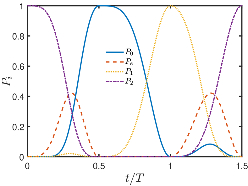
Figure 6: State populations $P_{i}$, $i=1,2,3,a$, versus the evolution time $t/T$ for the cyclic population transfer. The Rabi-frequencies $\Omega_{i}(t)$ and the phases $\varphi_{i}(t)$, $i=1,2,3,a$, are set according to Eqs. (42) and (43) with the parameters $\chi(t)$, $\phi(t)$, and $\theta(t)$ given in Eqs. (44), (45), and (46).

Using the outcome of the von Neumann equation including the phases in Eq. (42) and the Rabi frequencies in Eq. (43) with the stage-wise parameters $\chi(t)$, $\phi(t)$, and $\theta(t)$ given in Eqs. (44), (45), and (46), the population dynamics on the four levels $P_{i}$ are demonstrated in Fig. 6. It is found that the initial population on the state $|2\rangle$ can be completely transferred to $|0\rangle$ when $t=T/2$. And in this transfer process, the states $|1\rangle$ and $|e\rangle$ are temporally populated, i.e., $P_{1}=0.02$ and $P_{e}=0.42$ when $t=0.31T$. It is due to the fact that $|\mu_{2}(t)\rangle$ is a superposed state of all the four levels. Then at $t=T$, the population on the state $|0\rangle$ can be completely transferred to $|1\rangle$ via the path $|\mu_{0}(t)\rangle$. It is interesting to find that Stage $2$ is the same as that in the case of the three-level system. From $t=T$ to $t=3T/2$, the population on the state $|1\rangle$ is transferred back to $|2\rangle$ again along the path $|\mu_{2}(t)\rangle$.

When the system is initially prepared at $|0\rangle$ or $|1\rangle$, the preceding cyclic transfer could be preformed with only two stages. For example, if the cyclic loop is $|0\rangle\rightarrow|1\rangle\rightarrow|2\rangle\rightarrow|0\rangle$, then the first and second stages employ the paths $|\mu_{0}(t)\rangle$ and $|\mu_{2}(t)\rangle$, respectively. Along the path $|\mu_{0}(t)\rangle$ with $\theta(0)=0$ and $\theta(T)=\pi/2$, the system population can be transferred from $|0\rangle$ to $|1\rangle$. And then the population transfer $|1\rangle\rightarrow|e\rangle\rightarrow|0\rangle$ can be achieved along the path $|\mu_{2}(t)\rangle$ with $\chi(T/2)=0$, $\phi(T/2)=0$, $\theta(T/2)=0$, $\chi(T)=\pi/2$, $\phi(T)\rightarrow\phi$, $\theta(T)\rightarrow\theta$, $\chi(3T/2)=0$, $\phi(3T/2)=0$, and $\theta(3T/2)=\pi/2$.

V Conclusion

In Tab. 1, we summarize the common and distinct points between our universal protocol and the existing ones with respect to the state transfer in a three-level system, which is a popular example to show the control power only with three driving in Fig. 1. In addition to the adiabatic construction of the stable evolution path in STIRAP, one can demand a stable but fast evolution path via a nonadiabatic control method, e.g., our universal protocol that covers the methods of NHQT, LRT, CD and CDD. The full-rank nonadiabatic evolution operator obtained by our universal protocol allows to choose an arbitrary ancillary base as the state-transfer path. This versatility is superior to STIRAP and CD using $|\mu_{0}(t)\rangle$ and NHQT, LRT, and CDD using $|\mu_{1}(t)\rangle$ or $|\mu_{2}(t)\rangle$. One can also appreciate the utility of our protocol through the application in the cyclic population transfer.

In conclusion, we put forward a forward-engineering framework for nonadiabatic quantum control over the time-dependent systems within an ancillary picture. The instantaneous ancillary bases that satisfy the von Neumann equation under the system Hamiltonian provide nonadiabatic evolution paths for the interested system. There exists no transition among the qualified ancillary bases since the system Hamiltonian is diagonal in them. With a sufficient number of degrees of freedom in the time-dependent Hamiltonian, we can achieve a full-rank nonadiabatic evolution operator. It means that the Hamiltonian is fully diagonal in the parametric ancillary picture and then the system can be exactly solved. Our universal prescription supported by the von Neumann equation can unite many popular state-transfer protocols, including the nonadiabatic holonomic transformation, the Lewis-Riesenfeld theory for invariant, and the counterdiabatic driving methods. With a clear motivation and a convenient derivation, our protocol allows to construct a fast and stable path which connects arbitrary pairs of states for time-dependent quantum systems. And the rank of the obtained nonadiabatic evolution operator is constrained by the degrees of freedoms of the system.

More than highlighting the common basic elements of the existing protocols, our framework is useful in certain tasks of quantum control that is beyond the reach of them or greatly reduces the complexity in performance. Protocols about cyclic population transfer in a three-level system and a four-level system are presented, demonstrating the advantage of our framework in exploiting the potential of nonadiabatic control.

References

- Král et al. (2007) P. Král, I. Thanopulos, and M. Shapiro, Colloquium: Coherently controlled adiabatic passage, Rev. Mod. Phys. 79, 53 (2007).
- Zanardi and Rasetti (1999) P. Zanardi and M. Rasetti, Holonomic quantum computation, Phys. Lett. A 264, 94 (1999).
- Bergmann et al. (1998) K. Bergmann, H. Theuer, and B. W. Shore, Coherent population transfer among quantum states of atoms and molecules, Rev. Mod. Phys. 70, 1003 (1998).
- Gisin and Thew (2007) N. Gisin and R. Thew, Quantum communication, Nat. Photon. 1, 165 (2007).
- Kimble (2008) H. J. Kimble, The quantum internet, Nature 453, 1023 (2008).
- Dong et al. (2021) W. Dong, F. Zhuang, S. E. Economou, and E. Barnes, Doubly geometric quantum control, PRX Quantum 2, 030333 (2021).
- Berry (1984) M. V. Berry, Quantal phase factors accompanying adiabatic changes, Proc. R. Soc. Lond. A 392, 45 (1984).
- Aharonov and Anandan (1987) Y. Aharonov and J. Anandan, Phase change during a cyclic quantum evolution, Phys. Rev. Lett. 58, 1593 (1987).
- Wilczek and Zee (1984) F. Wilczek and A. Zee, Appearance of gauge structure in simple dynamical systems, Phys. Rev. Lett. 52, 2111 (1984).
- Anandan (1988) J. Anandan, Non-adiabatic non-abelian geometric phase, Phys. Lett. A 133, 171 (1988).
- De Chiara and Palma (2003) G. De Chiara and G. M. Palma, Berry phase for a spin particle in a classical fluctuating field, Phys. Rev. Lett. 91, 090404 (2003).
- Leek et al. (2007) P. J. Leek, J. M. Fink, A. Blais, R. Bianchetti, M. Göppl, J. M. Gambetta, D. I. Schuster, L. Frunzio, R. J. Schoelkopf, and A. Wallraff, Observation of berry’s phase in a solid-state qubit, Science 318, 1889 (2007).
- Filipp et al. (2009) S. Filipp, J. Klepp, Y. Hasegawa, C. Plonka-Spehr, U. Schmidt, P. Geltenbort, and H. Rauch, Experimental demonstration of the stability of berry’s phase for a spin- particle, Phys. Rev. Lett. 102, 030404 (2009).
- Cohen et al. (2019) E. Cohen, H. Larocque, F. Bouchard, F. Nejadsattari, Y. Gefen, and E. Karimi, Geometric phase from aharonov–bohm to pancharatnam–berry and beyond, Nat. Rev. Phys. 1, 437 (2019).
- Born and Fock (1928) M. Born and V. Fock, Beweis des adiabatensatzes, Z. Phys. 51, 165 (1928).
- Jones et al. (2000) J. A. Jones, V. Vedral, A. Ekert, and G. Castagnoli, Geometric quantum computation using nuclear magnetic resonance, Nature 403, 869 (2000).
- Duan et al. (2001) L.-M. Duan, J. I. Cirac, and P. Zoller, Geometric manipulation of trapped ions for quantum computation, Science 292, 1695 (2001).
- Sjöqvist et al. (2012) E. Sjöqvist, D. M. Tong, L. M. Andersson, B. Hessmo, M. Johansson, and K. Singh, Non-adiabatic holonomic quantum computation, New J. Phys. 14, 103035 (2012).
- Liu et al. (2019) B.-J. Liu, X.-K. Song, Z.-Y. Xue, X. Wang, and M.-H. Yung, Plug-and-play approach to nonadiabatic geometric quantum gates, Phys. Rev. Lett. 123, 100501 (2019).
- Zheng et al. (2016) S.-B. Zheng, C.-P. Yang, and F. Nori, Comparison of the sensitivity to systematic errors between nonadiabatic non-abelian geometric gates and their dynamical counterparts, Phys. Rev. A 93, 032313 (2016).
- Jing et al. (2017) J. Jing, C.-H. Lam, and L.-A. Wu, Non-abelian holonomic transformation in the presence of classical noise, Phys. Rev. A 95, 012334 (2017).
- Claridge (2009) T. D. W. Claridge, High-Resolution NMR Techniques in Organic Chemistry (Elsevier New York, 2009).
- Vitanov et al. (2017) N. V. Vitanov, A. A. Rangelov, B. W. Shore, and K. Bergmann, Stimulated raman adiabatic passage in physics, chemistry, and beyond, Rev. Mod. Phys. 89, 015006 (2017).
- Pillet et al. (1993) P. Pillet, C. Valentin, R.-L. Yuan, and J. Yu, Adiabatic population transfer in a multilevel system, Phys. Rev. A 48, 845 (1993).
- Phillips (1998) W. D. Phillips, Nobel lecture: Laser cooling and trapping of neutral atoms, Rev. Mod. Phys. 70, 721 (1998).
- García-Ripoll and Cirac (2003) J. J. García-Ripoll and J. I. Cirac, Quantum computation with unknown parameters, Phys. Rev. Lett. 90, 127902 (2003).
- Daems and Guérin (2007) D. Daems and S. Guérin, Adiabatic quantum search scheme with atoms in a cavity driven by lasers, Phys. Rev. Lett. 99, 170503 (2007).
- Jing et al. (2016) J. Jing, M. S. Sarandy, D. A. Lidar, D.-W. Luo, and L.-A. Wu, Eigenstate tracking in open quantum systems, Phys. Rev. A 94, 042131 (2016).
- Chen et al. (2010a) X. Chen, I. Lizuain, A. Ruschhaupt, D. Guéry-Odelin, and J. G. Muga, Shortcut to adiabatic passage in two- and three-level atoms, Phys. Rev. Lett. 105, 123003 (2010a).
- Guéry-Odelin et al. (2019) D. Guéry-Odelin, A. Ruschhaupt, A. Kiely, E. Torrontegui, S. Martínez-Garaot, and J. G. Muga, Shortcuts to adiabaticity: Concepts, methods, and applications, Rev. Mod. Phys. 91, 045001 (2019).
- Baksic et al. (2016) A. Baksic, H. Ribeiro, and A. A. Clerk, Speeding up adiabatic quantum state transfer by using dressed states, Phys. Rev. Lett. 116, 230503 (2016).
- Li and Chen (2016) Y.-C. Li and X. Chen, Shortcut to adiabatic population transfer in quantum three-level systems: Effective two-level problems and feasible counterdiabatic driving, Phys. Rev. A 94, 063411 (2016).
- Chen et al. (2010b) X. Chen, A. Ruschhaupt, S. Schmidt, A. del Campo, D. Guéry-Odelin, and J. G. Muga, Fast optimal frictionless atom cooling in harmonic traps: Shortcut to adiabaticity, Phys. Rev. Lett. 104, 063002 (2010b).
- Chen et al. (2011) X. Chen, E. Torrontegui, and J. G. Muga, Lewis-riesenfeld invariants and transitionless quantum driving, Phys. Rev. A 83, 062116 (2011).
- Chen and Muga (2012) X. Chen and J. G. Muga, Engineering of fast population transfer in three-level systems, Phys. Rev. A 86, 033405 (2012).
- Qi and Jing (2022) S.-f. Qi and J. Jing, Accelerated adiabatic passage in cavity magnomechanics, Phys. Rev. A 105, 053710 (2022).
- Berry (2009) M. V. Berry, Transitionless quantum driving, J. Phys. A 42, 365303 (2009).
- Koch et al. (2007) J. Koch, T. M. Yu, J. Gambetta, A. A. Houck, D. I. Schuster, J. Majer, A. Blais, M. H. Devoret, S. M. Girvin, and R. J. Schoelkopf, Charge-insensitive qubit design derived from the cooper pair box, Phys. Rev. A 76, 042319 (2007).
- Vepsäläinen et al. (2019) A. Vepsäläinen, S. Danilin, and G. S. Paraoanu, Superadiabatic population transfer in a three-level superconducting circuit, Sci. Adv. 5, eaau5999 (2019).