Multitype entanglement dynamics induced by exceptional points

Abstract

As a most important feature of non-Hermitian systems, exceptional points (EPs) lead to a variety of unconventional phenomena and applications. Here we discover that multitype entanglement dynamics can be induced by engineering different orders of EP. By studying a generic model composed of two coupled non-Hermitian qubits, we find that diverse entanglement dynamics on the two sides of the fourth-order EP (EP4) and second-order EP (EP2) can be observed simultaneously in the weak coupling regime. With the increase of the coupling strength, the EP4 is replaced by an additional EP2, leading to the disappearance of the entanglement dynamics transition induced by EP4 in the strong coupling regime. Considering the case of Ising type interaction, we also realize EP-induced entanglement dynamics transition without the driving field. Our study paves the way for the investigation of EP-induced quantum effects and applications of EP-related quantum technologies.

I Introduction

Non-Hermitian (NH) Hamiltonians provide an effective method to describe physical systems that exchange energy, information or particles with the environment Bender and Boettcher (1998); Heiss (2004). For instance, NH Hamiltonians have been applied to describe optical Rüter et al. (2010); El-Ganainy et al. (2018); Hodaei et al. (2017), acoustic Zhu et al. (2018); Liu et al. (2018) and magnetic systems Yang et al. (2020); Wang et al. (2019) with gain and loss or asymmetric couplings. These non-Hermitian systems have unprecedented features induced by non-HermiticityBender and Boettcher (1998). As a most peculiar example, exceptional points (EPs) describe the coalescence of the eigenstates and the degeneracy of the eigenvalues, indicating the phase transition from the parity-time ($\mathcal{PT}$) symmetric phase to the $\mathcal{PT}$-symmetry-broken phase Heiss (2004); Bergholtz et al. (2021); Özdemir et al. (2019); Parto et al. (2021); Miri and Alù (2019). EPs play an important role in many remarkable physical phenomena and functional applications. For example, the nonlinear perturbation response of EPs induces a variety of unconventional effects, including nonreciprocal light propagation Peng et al. (2014a); Chang et al. (2014), loss-induced transparency Peng et al. (2014b); Zhang et al. (2018) and coherent perfect absorption Sun et al. (2014); Wang et al. (2021), making them promising platforms for wireless power transfer Assawaworrarit and Fan (2020); Assawaworrarit et al. (2017), single-mode lasers Feng et al. (2014) and so on.

In addition to investigating EPs in classical systems, the extension of EPs to quantum regime has attracted much attention. Based on the methods of extended Hilbert space Wu et al. (2019) and quantum trajectories Naghiloo et al. (2019) to construct effective NH Hamiltonians, EPs have been achieved in various quantum platforms such as dissipative photon systems Xiao et al. (2020); Öztürk et al. (2021), superconducting circuits Naghiloo et al. (2019); Chen et al. (2021); McDonald and Clerk (2020); Chen et al. (2022), single ion traps Ding et al. (2021), thermal atom ensembles Cao et al. (2020); Liang et al. (2023), cold atoms Li et al. (2019); Lee and Chan (2014) and nitrogen-vacancy color-centers Wu et al. (2019); Pick et al. (2019). Quantum effects including photon blockadeHuang et al. (2022); Li et al. (2023a); Zuo et al. (2022); Yuan et al. (2023) and topological quantum state controlLiu et al. (2021); Gong et al. (2018); Xu et al. (2016) have been achieved by engineering the EPs. As a most important quantum property, EP-induced exceptional entanglement behaviors have also been observed in very recent works. For example, the occurrence of the entanglement transition at the EP has been observed in a NH system composed of qubit coupled with photonsHan et al. (2023). Entanglement generation between two NH qubits can be accelerated by approaching the EP of the systemLi et al. (2023b). Replacing one NH qubit with unitary qubit, entanglement can be maximized at the EPKumar et al. (2022). However, since most work have only discussed the case of second-order EPs, the relationship between the orders of EPs and entanglement remains unknown.

Here, we show that multitype entanglement dynamics can be realized by engineering different orders of EPs, by analyzing a generic model composed of two coupled NH qubits. The inter-qubit coupling will lower the order of EP from the original fourth-order EP (EP4) to a second-order EP (EP2). However, we find that disparate entanglement dynamics on the two sides of the original EP4 and EP2 can be observed simultaneously in the case of weak coupling (i.e., the coupling strength is much smaller than the dissipation rate), indicating different types of entanglement behaviors can be induced by tuning the order of EP. When enhancing the coupling strength to the strong coupling regime (i.e., the coupling strength and dissipation rate are on the same order), the original EP4 is replaced by an additional EP2, leading to the disappearance of the EP4-engineered entanglement transition. Taking Ising type interaction as an example, we also find EP-induced entanglement transition in the absence of the driving field. Our scheme is universal for a variety of quantum systems, such as superconducting circuits Blais et al. (2020); Xiang et al. (2013); Devoret and Schoelkopf (2013) and ion traps Monroe and Kim (2013); Pino et al. (2021). This study paves the way for the investigation of quantum effects induced by EPs, and provides opportunities for designing EP-based quantum devices.

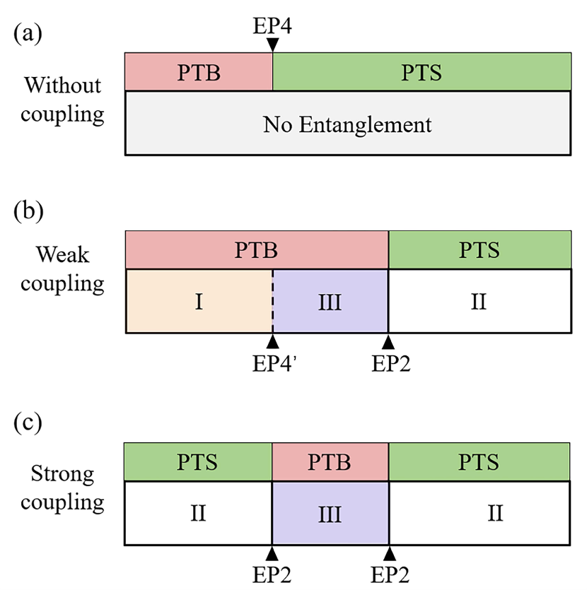
Figure 1: Schematic diagram of the multitype entanglement dynamics (I, II, III) induced by EPs with different orders. The regions of PTB and PTS represent the $\mathcal{P}\mathcal{T}$-symmetry-broken phase and the $\mathcal{P}\mathcal{T}$-symmetric phase, respectively. (a) The system exhibits a fourth-order EP (EP4) without coupling and no entanglement will be generated in this case. (b) In the weak coupling regime (the coupling strength $\xi$ is much smaller than the dissipation rate $\gamma$ of the qubits, i.e., $\xi\ll\gamma$), the system exhibits the original EP4 ($\text{EP}4^{\prime}$) and an existing second-order EP (EP2). (c) In the strong coupling regime (i.e, $\xi\sim\gamma$), the original EP4 disappears and an additional EP2 will emerge. The definition of type I, II and III denote three different types of entanglement dynamics. The entanglement behavior of type I is monotonically increasing and eventually reaching a stable value, type II corresponds to the entanglement behavior of continuous oscillations over the entire time domain, and type III combines the characteristics of the above two different entanglement behaviors.

II Model

We consider a generic system composed of two coupled NH qubits (or spin). The type of interaction can be treated as either dipolar or Ising type interaction. The system Hamiltonian is given as ($\hbar=1$)

$$H=\sum\limits_{j=1,2}{\left({{\delta}_{j}}-\frac{i{{\gamma}_{j}}}{2}\right)\sigma_{j}^{-}}\sigma_{j}^{+}+{{\Omega}_{j}}\sigma_{j}^{x}+{{H}_{\operatorname{int}}},$$ (1)

where ${{\delta}_{j}}$ represents the frequency detuning of the driving field from the qubit transition frequency, ${{\gamma}_{j}}$ and ${{\Omega}_{j}}$ is the energy decay rate of ${{\left|b\right\rangle}_{j}}$ and driving amplitude, respectively. The Pauli operators in terms of the quantum energy levels-with no classical analogs- ${{\left|b\right\rangle}_{j}}$ and ${{\left|a\right\rangle}_{j}}$ as $\sigma_{j}^{+}={{\left|a\right\rangle}_{j}}\left\langle b\right|,\sigma_{j}^{-}={{\left|b\right\rangle}_{j}}\left\langle a\right|$ and $\sigma_{j}^{x}={{\left|b\right\rangle}_{j}}\left\langle a\right|+{{\left|a\right\rangle}_{j}}\left\langle b\right|,j\in\{1,2\}$. In the following analysis, we take ${{\gamma}_{1}}={{\gamma}_{2}}=\gamma$ and ${{\Omega}_{1}}={{\Omega}_{2}}=\Omega$ for simplicity and assumed that ${{\delta}_{j}=0}$ (i.e., the drives are resonant with two qubits). The third term represents the interaction between the two NH qubits. When the two qubits are coupled via dipolar interaction, the Hamiltonian can be described as ${{H}_{\operatorname{int}}}=g\left(\sigma_{1}^{\dagger}{{\sigma}_{2}}+{{\sigma}_{1}}\sigma_{2}^{\dagger}\right)$, which can be realized in various systems such as superconducting circuit systems Naghiloo et al. (2019); Dalmonte et al. (2015) and Rydberg atom systems de Léséleuc et al. (2019). In addition to this interaction type, there is another type of interaction between the two qubits or spins, i.e, Ising type interaction, which can be represented as ${{H}_{\operatorname{int}}}=-\xi{{\left(\sigma_{x}^{1}+\sigma_{x}^{2}\right)}^{2}}$. Here $g$ and $\xi$ denote the coupling strength, respectively. Ising type interaction has been widely studied in hybrid spin-mechanical system Pan et al. (2023); Li et al. (2016), the quantum spin lattice systems Dür et al. (2005); Britton et al. (2012) and hybrid circuit systemsBohnet et al. (2016); Block et al. (2022).

III EPs with different orders

In the following we mainly focus on the case of Ising type interaction (the calculation of the dipolar interaction case can be found in Sec. VI). Due to ${{\delta}_{j}=0}$, the system Hamiltonian in Eq. (1) reduces to a so-called passive $\mathcal{P}\mathcal{T}$-symmetric Hamiltonian Guo et al. (2009) can be written as $H={{H}_{\mathcal{PT}}}-\left(i\gamma/2\right)I$ with $I$ being the unitary matrix. The Hamiltonian ${{H}_{\mathcal{PT}}}$ can be written as

$$\begin{split}{{H}_{\mathcal{PT}}}=&\left(\begin{matrix}J+\frac{i\gamma}{2}&\Omega&\Omega&J\\ \Omega&J&J&\Omega\\ \Omega&J&J&\Omega\\ J&\Omega&\Omega&J-\frac{i\gamma}{2}\\ \end{matrix}\right),\end{split}$$ (2)

where $J=-2\xi$. $H_{\mathcal{PT}}$ satisfies $\mathcal{P}\mathcal{T}$ symmetry, where the parity operator is given as $\mathcal{P}=\sigma_{1}^{x}\sigma_{2}^{x}$.

The eigenvalues of the system without coupling, i.e., $\xi=0$ ($g=0$), are ${{\lambda}_{0,1}}=-i\gamma/2$ and ${{\lambda}_{\pm}}=-i\gamma/2\pm i\sqrt{16{{\Omega}^{2}}-{{\gamma}^{2}}}/2$, indicating the system exists a four-order EP (EP4) if $\Omega={{\Omega}_{\text{EP4}}}=\gamma/4$ [Fig. 2(a) and  2(d)]. The region of $\mathcal{P}\mathcal{T}$-symmetric phase (PTS) ($\Omega>{{\Omega}_{\text{EP4}}}$) is on the right-hand side of the EP4 while the region of $\mathcal{P}\mathcal{T}$-symmetry-broken phase (PTB) ($\Omega<{{\Omega}_{\text{EP4}}}$) is on the left-hand side of the EP4 [Fig. 1(a)]. The order of EP will be lowered from 4 to 2 when adding the qubit-qubit coupling. As shown in Fig. 2(b) and  2(e), an EP2 can be found at ${{\Omega}_{\text{EP2}}}/\gamma=0.283$ when choosing $\xi/\gamma=0.006$ as an example. In the weak coupling regime (i.e., $\xi\ll\gamma$), the coupling can also be considered as a perturbation. The original EP4 (${{\Omega}_{\text{EP}4^{\prime}}}={{\Omega}_{\text{EP}4}}$) and existing EP2 will form a new phase (${{\Omega}_{\text{EP4}^{\prime}}}<\Omega<{{\Omega}_{\text{EP2}}}$)[Fig. 1(b)], as different entanglement dynamics can be observed in this region, which will be mainly discussed in the following section. Interestingly, an additional EP2 will appear in the system when enhancing the coupling strength to the strong coupling regime (i.e., $\xi\sim\gamma$). As demonstrated in Fig. 2(c) and  2(f), one EP2 appears at the critical value $\Omega_{\text{EP2}}^{(1)}/\gamma=0.626$ and an additional EP2 is at $\Omega_{\text{EP2}}^{(2)}/\gamma=1.34$ when choosing $\xi/\gamma=0.5$. The region of PTB occurs at $\Omega_{\text{EP2}}^{(1)}<\Omega<\Omega_{\text{EP2}}^{(2)}$ and the regions of PTS take place at $\Omega<\Omega_{\text{EP2}}^{(1)}$ and $\Omega>\Omega_{\text{EP2}}^{(2)}$ [Fig. 1(c)].

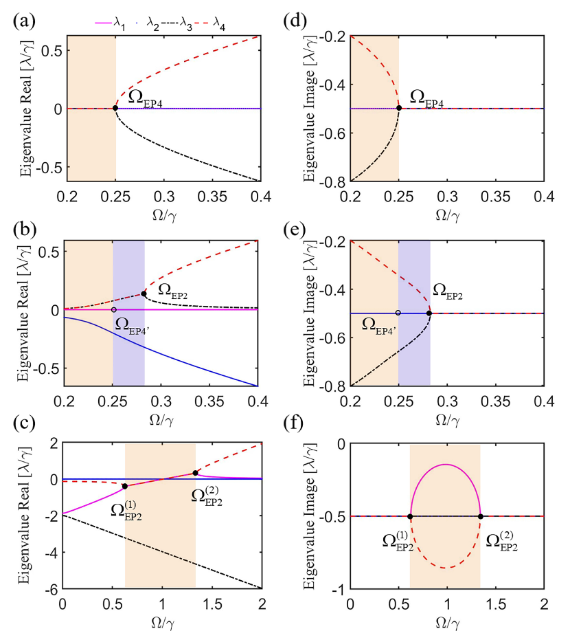
Figure 2: Real (a, b, c) and imaginary (d, e, f) parts of eigenvalues for different Ising type interaction strength. (a) Real and (d) imaginary parts of the eigenvalues for $\xi/\gamma=0$. And examples for weak coupling regime for $\xi/\gamma=0.006$ (b, e) and strong coupling regime for $\xi/\gamma=0.5$ (c, f), respectively. The two qubits are assumed to have the same drive amplitude $\Omega$ and the same decay rates $\gamma$. The orange and white regions represent the PTB and PTS, respectively. The new phase is formed by the original EP4 and existing EP2 (i.e., ${{\Omega}_{\text{EP4}^{\prime}}}<\Omega<{{\Omega}_{\text{EP2}}}$) in the case of weak coupling is illustrated in the blue region.

IV Different entanglement dynamics

The state evolution of the coupled NH qubits can be obtained by solving the equation of motion

$$\frac{d\rho}{dt}=-i\left(H\rho-\rho{{H}^{\dagger}}\right)$$ (3)

where $H$ is the non-Hermitian system Hamiltonian [Eq. (1)] and $\rho$ denotes the density matrix of the system. To describe the entanglement between the two NH qubits, we calculate the concurrence as Wootters (1998)

$$C=\max\left({{\tau}_{1}}-{{\tau}_{2}}-{{\tau}_{3}}-{{\tau}_{4}},0\right).$$ (4)

Here ${{\tau}_{1}}$, ${{\tau}_{2}}$, ${{\tau}_{3}}$, ${{\tau}_{4}}$ are the eigenvalues of the Hermitian matrix $R=\sqrt{\sqrt{\rho}\widetilde{\rho}\sqrt{\rho}}$, with $\widetilde{\rho}=\left({{\sigma}_{y}}\otimes{{\sigma}_{y}}\right){{\rho}^{*}}\left({{\sigma}_{y}}\otimes{{\sigma}_{y}}\right)$ in decreasing order and ${{\sigma}_{y}}=-i\left|b\right\rangle\left\langle a\right|+i\left|a\right\rangle\left\langle b\right|$.

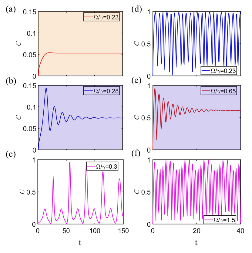
Figure 3: The concurrence evolution in the region of PTB (a), the new phase (b) and PTS (c) in the case of weak coupling $\xi/\gamma=0.006$. The original EP4 induce the exceptional entanglement phenomena on the two sides of this point. In the strong coupling regime for $\xi/\gamma=0.5$, the EP2 induces different entanglement behavior on the two sides of $\Omega/\gamma=0.626$, i.e., in the region of PTS (d, f) and PTB (e). The initial state is $\left|\psi(0)\right\rangle=\left|aa\right\rangle$.

Assuming the initial state of the two coupled NH qubits is $\left|\psi(0)\right\rangle=\left|aa\right\rangle$, the concurrence evolution in both the weak [Fig. 3(a),  3(b) and  3(c)] and strong coupling regime [Fig. 3(d),  3(e) and  3(f)] can be obtained numerically. The entanglement behaviors are significantly different when tuning different parameters. In the case of weak coupling (taking $\xi/\gamma=0.006$ as an example), the degree of entanglement is weak and monotonically increases until evolving to a stable value in the region of $\Omega<{{\Omega}_{\text{EP4}^{\prime}}}$ [Fig. 3(a)]. We define this type of entanglement dynamics as type I, which can only be observed in the weak coupling regime. With increasing the driving amplitude to the second region, i.e., ${{\Omega}_{\text{EP4}^{\prime}}}<\Omega<{{\Omega}_{\text{EP2}}}$, the entanglement dynamics exhibits a combination function of decay and oscillation, reaching to a fixed value of concurrence at the steady state [Fig. 3(b)]. Clearly, this type of entanglement dynamics is different from the type I, which we defined as type III.

According to the results in Fig. 3(a) and  3(b), we can find that the entanglement behaviors are absolutely different when crossing the orginal EP4, which indicates that the entanglement dynamics transition is induced by the original EP4, although the original EP4 is absent in the presence of coupling. It is necessary to define this particular region where enclosed by the original EP4 and EP2 as a new phase, as the blue region shown in Fig. 1(b). This new phase is a part of the PTB.

In the region of PTS, i.e., $\Omega>{{\Omega}_{\text{EP2}}}$, the entanglement dynamics exhibits continuous oscillation in the whole time-evolution process [Fig. 3(c)], which is defined as type II. The maximum entanglement ($C=1$) can be obtained in the oscillation process and the degree of entanglement in PTS is much larger than that in PTB. By using the theory of time-independent perturbation theory for non-Hermitian systems Li et al. (2023b), we can obtain the analytical results of the concurrence in the weak coupling regime, which shows a good agreement with the numerical results in the $\mathcal{P}\mathcal{T}$-symmetric phase (see Appendix C.3 for more details). The multitype entanglement dynamics (type I, II, III) as described above can also be seen in the aspect of the population of the basis state. The normalized quantum state can be expressed as $\left|\widetilde{\psi}\right\rangle=\alpha\left|aa\right\rangle+\beta\left|ab\right\rangle+\zeta\left|ba\right\rangle+\delta\left|bb\right\rangle$. Hence the concurrence is given by $C=2\left|\alpha\delta-\beta\zeta\right|$. corresponding to the population at each basis state exhibits different oscillatory behaviors in the three phases divided by the original EP4 and EP2 (as shown in Fig. 4), different entanglement dynamics can be found in the three phases, accordingly.

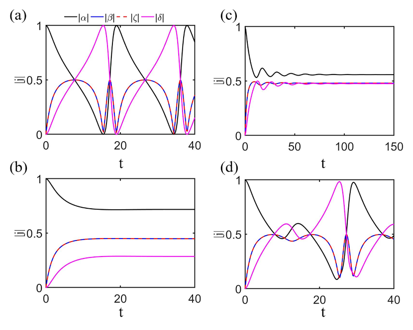
Figure 4: Time evolution of the modulus $\left|j\right|(j=\alpha,\beta,\varsigma,\delta)$ for each of the four complex amplitudes of the two-qubit state $\left|\widetilde{\psi}\right\rangle=\alpha\left|aa\right\rangle+\beta\left|ab\right\rangle+\zeta\left|ba\right\rangle+\delta\left|bb\right\rangle$ for $\xi=0$ (a) and $\xi/\gamma=0.006$ (b-d). In the absence of Ising interaction, the evolution of $\left|j\right|$ is focused in the $\mathcal{P}\mathcal{T}$-symmetric phase. In the presence of Ising interaction, the evolution of $\left|j\right|$ has been shown in three different regions, i.e., in the $\mathcal{P}\mathcal{T}$-symmetry-broken phase (b), the new phase (c) and $\mathcal{P}\mathcal{T}$-symmetric phase (d), respectively. The given driving amplitude are chosen as $\Omega/\gamma=0.23$ (b), $\Omega/\gamma=0.28$ (c) and $\Omega/\gamma=0.3$ (d).

Compared with the the populations evolution of the basis states $\left|bb\right\rangle$ and $\left|aa\right\rangle$ in the three different phases, we can find that the distorted Rabi-like oscillation of the population of $\left|bb\right\rangle$ and $\left|aa\right\rangle$ in the PTS, as the black and pink curves shown in Fig. 4(a) and  4(d) regardless of whether there exists interaction. Moreover, the population evolution of the states $\left|ab\right\rangle$ and $\left|ba\right\rangle$ monotonically increase during the system evolving to a steady state in the PTB [Fig. 4(b)] and the new phase [Fig. 4(c)]. Strikingly, the populations evolution of the basis states $\left|bb\right\rangle$ and $\left|aa\right\rangle$ are oscillations at short timescale and finally reach to a steady state in the new phase, which are different from that in the PTB. The different populations evolution corresponds to the distinctive entanglement dynamics in the region of new and PTB. In addition, we note that at specific time ${{T}^{*}}=27.2$, the populations of basis state are equal, i.e., $\left|\alpha\right|\sim\left|\beta\right|\sim\left|\varsigma\right|\sim\left|\delta\right|$.

With the increase of the coupling strength to the strong coupling regime, i.e., $\xi/\gamma=0.5$ as an example, the original EP4 is replaced by another EP2, which means there are two different EP2s in the system [see Fig. 2(c) and  2(f)]. The entanglement between two coupled NH qubits has been shown in Fig. 3(d),  3(e) and  3(f). We can observe that the entanglement dynamics of type II takes place both in the region of $\Omega<\Omega_{\text{EP2}}^{(1)}$ and $\Omega>\Omega_{\text{EP2}}^{(2)}$, i.e., the region of PTS, as shown in Fig. 3(d) and  3(f), respectively. In PTB, i.e., $\Omega_{\text{EP2}}^{(1)}<\Omega<\Omega_{\text{EP2}}^{(2)}$, the entanglement dynamics is the same as the defined type III as demonstrated in Fig. 3(e). Therefore, only two types of entanglement dynamics can be found in the strong coupling regime. When calculating the entanglement dynamics in the regions near the two sides of the original EP4 ($\Omega/\gamma=0.25$), which behaves almost consistent (see Fig. 5(a) and  5(b)). It means that due to the replacement of the original EP4 with another EP2, entanglement dynamics of type I will not appear in the strong coupling regime. The impact of original EP4 on entanglement disappears, which also indicates that the new phase vanishes.

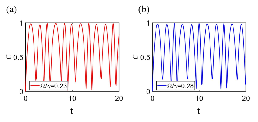
Figure 5: Concurrence evolution for the critical values near the original EP4 in the strong coupling regime. As an example, for $\Omega/\gamma=0.23$ (a) and $\Omega/\gamma=0.28$ (b) in the left and right sides near the original EP4, respectively.

The effect of the original EP4 on entanglement dynamics are completely different in the weak and strong coupling regime. The presence of the weak coupling can be considered as a perturbation, such that the original EP4 still makes a significant influence on the parameter space, leading to a different entanglement dynamics on the two sides near the original EP4. However, when the coupling strength is large enough, the contribution of the strong coupling on the parameter space is dominant, leading to the disappearance of the entanglement dynamics transition induced by the original EP4. Therefore, the coexistence of the two EPs with different orders, i.e., EP4 and EP2, can induce three different types of entanglement dynamics in the weak coupling regime. Depend on the same order of the two EP2s, only a jump of entanglement dynamics can be found in the strong coupling regime.

V Entanglement transition without the driving field

In the absence of the driving field applied to the qubits, i.e., ${{\Omega}_{i=1,2}}=0$. Exceptional entanglement transition can also occur when considering the Ising type interaction. The Hamiltonian with Ising type interaction evolves within the subspace $\left\{\left|{{a}_{1}},{{a}_{2}}\right\rangle,\left|{{a}_{1}},{{b}_{2}}\right\rangle,\left|{{a}_{2}},{{b}_{1}}\right\rangle,\left|{{b}_{1}},{{b}_{2}}\right\rangle\right\}$. With a correction of the quantum state distortion caused by the decoherence, the evolution of the joint probability $\left|{{b}_{1}},{{b}_{2}}\right\rangle$, denoted as ${{P}_{{{b}_{1}}{{b}_{2}}}}$, indicating the quantum Rabi oscillator signal. Figure 6(a) and  6(b) show the obtained ${{P}_{{{b}_{1}}{{b}_{2}}}}$ as functions of time in the regions of different phases. Specifically, in PTB (e.g., $\xi/\gamma=-0.16$), the population of state $\left|{{b}_{1}},{{b}_{2}}\right\rangle$ monotonically decays during the system evolving to a steady state [Fig. 6(a)]. After crossing the EP, i.e., in the region of PTS (e.g., $\xi/\gamma=-0.5$), the state population ${{P}_{{{b}_{1}}{{b}_{2}}}}$ presents a distinct oscillatory behavior in time evolution as shown in Fig. 6(b).

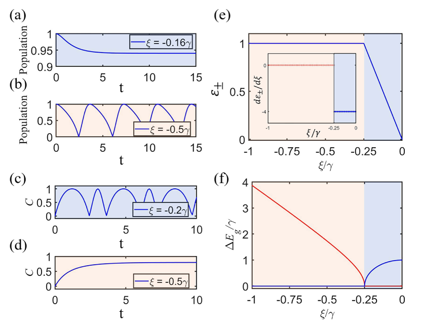
Figure 6: Observation of exceptional phase transitions in the absence of $\Omega$. (a) and (b) Measured evolution of the population of the basis state $\left|{{b}_{1}},{{b}_{2}}\right\rangle$ in PTB (for $\xi/\gamma=-0.16$) and PTS (for $\xi/\gamma=-0.5$), respectively. Concurrence evolution are given for $\xi=-0.2\gamma$ (c) and $\xi=-0.5\gamma$ (d). (e) Concurrence values ${{\varepsilon}_{\pm}}$ for the eigenstates $\left|{{\Phi}_{+}}\right\rangle$ and $\left|{{\Phi}_{-}}\right\rangle$ versus the Ising type interaction strength $\xi$. The derivatives $d{{\varepsilon}_{\pm}}/d\xi$ around the EP2, obtained by $\left[{{\varepsilon}_{\pm}}(\xi+\delta\xi)-{{\varepsilon}_{\pm}}(\xi)\right]/d\xi$, as shown in the insets. (f) Spectral gap $\Delta{{E}_{g}}$. As the eigenspectrum is possessed the entangled eigenstates of the two qubits system. This gap corresponds to the vacuum Rabi splitting.

To show the relationship between entanglement behavior and the EP, we give the concurrence evolution for $\xi=-0.2\gamma$ and $-0.5\gamma$ in Fig. 6(c) and  6(d), respectively. The result demonstrates that the entanglement exhibits different evolution behaviors in PTB and PTS. Figure 6(e) indicates the concurrence values ${{\varepsilon}_{\pm}}$ associated with the two eigenstates $\left|{{\Phi}_{\pm}}\right\rangle$ of the system as functions of $\xi$. As theoretical predicted, below the EP (i.e., $\left|\xi/\gamma\right|>{\gamma}/{4}\;$), the concurrence value of each eigenstate is saturated and approximately converge to the same maximally entangled state (reaching the maximum value 1) and independent of $\xi$ until at the EP $\xi=-\gamma/4$, where the energy gap disappeared. The expression of the concurrence has been given in Appendix A. The discontinuity of these derivatives indicates the occurrence of an entanglement transition at the EP, which are shown in the insets. After crossing the EP (i.e., $\left|\xi/\gamma\right|<{\gamma}/{4}\;$), the concurrence values ${{\varepsilon}_{\pm}}$ exhibit a linear scaling and depends on $\xi$. ${{\varepsilon}_{\pm}}$ are decreasing to 0 with the reduce of $\left|\xi\right|$. In Fig. 6(f), the energy gap described as ${{E}_{g}}=\sqrt{4{{J}^{2}}-{{\gamma}^{2}}}$ with $J=-2\xi$, undergoes a transition from the real part to the imaginary part at the EP, which is accompanied by an entanglement transition of the eigenstates. In addition, according to the results in Fig. 6(a), 6(b) and  6(e), this type of the energy gap transition also accompanied by the effect of the vacuum Rabi splitting of the entangled states.

VI The calculation for the system with dipolar interaction

In addition to the case of the Ising type interaction discussed above, we also considered the dipolar interaction between the qubits, which can be given by

$${{H}_{\operatorname{int}}}=g(\sigma_{1}^{+}\sigma_{2}^{-}+\sigma_{1}^{-}\sigma_{2}^{+}).$$ (5)

We defined $g$ as the effective dipolar interaction between the two qubits. In this case, the matrix of the total Hamiltonian can be written as

$$H=\begin{pmatrix}0&\Omega&\Omega&0\\ \Omega&-i\frac{\gamma}{2}&g&\Omega\\ \Omega&g&-i\frac{\gamma}{2}&\Omega\\ 0&\Omega&\Omega&g-i\gamma\\ \end{pmatrix}.$$ (6)

We now investigate the EP properties of the system where the two qubits are coupled with dipolar coupling. By numerically solving the matrix of the Hamiltonian Eq. (6), we can obtain the eigenvalues of the system, as shown in Figure 7. In the weak coupling regime (i.e., $g\ll\gamma$) for $g/\gamma=0.006$, there exists an EP2 at $\Omega/\gamma=0.283$ [Fig. 7(a) and  7(b)]. And the EP2 appears at $\Omega/\gamma=0.47$ in the strong coupling regime (i.e., $g\sim\gamma$) for $g/\gamma=0.5$ [Fig. 7(c) and  7(d)].

The $\mathcal{P}\mathcal{T}$-symmetry-broken phase is in the region of $\Omega<{{\Omega}_{\text{EP4}^{\prime}}}$ while the new phase is in the region of ${{\Omega}_{\text{EP4}^{\prime}}}<\Omega<{{\Omega}_{\text{EP2}}}$. It is worth to note that the new phase belongs to the $\mathcal{P}\mathcal{T}$-symmetry-broken phase. Different from the case of Ising type interaction, there is only a single EP2 in the strong coupling regime for the case of dipolar interaction.

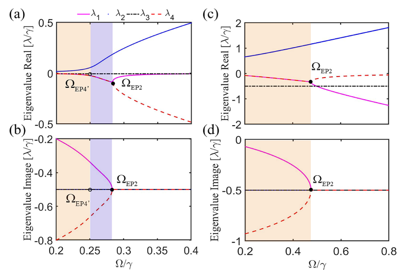
Figure 7: Real (a, c) and imaginary (b, d) parts of eigenvalues for different dipolar coupling regimes as $g/\gamma=0.006$ (a, b) in the weak coupling regime (i.e., $g\ll\gamma$) and $g/\gamma=0.5$ (c, d) in the strong coupling regime (i.e., $g\sim\gamma$), respectively. The two qubits are assumed to have the same drive amplitude $\Omega$ and the same decay rates$\gamma$. The orange, blue and white regions represent the $\mathcal{P}\mathcal{T}$-symmetry-broken phase, the new phase and $\mathcal{P}\mathcal{T}$-symmetric phase, respectively. The value of original EP4 is at the critical point ${{\Omega}_{\text{EP4}^{\prime}}}={{\Omega}_{\text{EP4}}}=\gamma/4$.

For the weak coupling regime, we can find that different entanglement dynamics on the two sides near the original EP4 and EP2 can be observed simultaneously, as shown in Fig. 8(a)-Fig. 8(c). These phenomena show that the different types of entanglement behaviors can still be induced by tuning the order of EP. In the strong coupling regime, the EP2-engineered entanglement transition is still existing [see Fig. 8(d) and  8(e)], but the influence of original EP4 on entanglement behavior is disappeared, as shown in Fig. 8(f). Similar with the results in the case of Ising type interaction, the type I of entanglement behavior only takes place in the weak coupling regime.

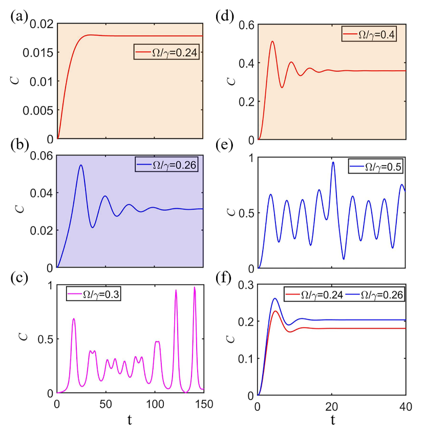
Figure 8: For the case of dipolar interaction, the concurrence evolution in the $\mathcal{P}\mathcal{T}$-symmetry-broken phase (a), the new phase (b) and $\mathcal{P}\mathcal{T}$-symmetric phase (c) for weak coupling strength $\xi/\gamma=0.006$. The virtual EP4 induce the exceptional entanglement phenomena on the two sides of this point. In the strong coupling regime for $\xi/\gamma=0.5$, the EP2 induces different entanglement behavior on the two sides of ${{\Omega}_{\text{EP2}}}/\gamma=0.47$, i.e., in the $\mathcal{P}\mathcal{T}$-symmetry-broken phase (d) and $\mathcal{P}\mathcal{T}$-symmetric phase (e). (f) The entanglement dynamics for the driving amplitude $\Omega/\gamma=0.24,0.26$. The initial state is $\left|\psi(0)\right\rangle=\left|aa\right\rangle$.

VII Conclusions

In conclusion, we have discovered multitype entanglement dynamics can be induced by engineering different orders of EP in the system with two coupled NH qubits. It can be found that different entanglement dynamics on the two sides near the original EP4 and EP2 can be observed simultaneously in the weak coupling regime. Moreover, the original EP4-engineered entanglement dynamics only exists in the weak coupling regime and will disappear in the strong coupling regime due to the absence of EP4. We have also demonstrated that an EP-enabled entanglement transition in the system without the driving amplitude in the case of Ising type interaction. Our work provides a protocol for exploring the connection between the entanglement and higher-order EPs, offering opportunities for designing quantum devices by engineering EPs.

Appendix A The concurrence for the two qubits without the driving amplitude

For the eigenstates $\left|{{\Phi}_{\pm}}\right\rangle$ of the Hamiltonian without the driving term, the system density operator in the basis states $\left|{{b}_{1}},{{b}_{2}}\right\rangle$ ,$\left|{{b}_{1}},{{a}_{2}}\right\rangle,\left|{{a}_{1}},{{b}_{2}}\right\rangle,\left|{{a}_{1}},{{a}_{2}}\right\rangle$ can be expressed as

$${{\rho}_{\pm}}={{\left|{{N}_{\pm}}\right|}^{2}}\left(\begin{matrix}{{J}^{2}}&0&0&J{{\Gamma}_{\pm}}\\ 0&0&0&0\\ 0&0&0&0\\ J\Gamma_{\pm}^{*}&0&0&{{\left|{{\Gamma}_{\pm}}\right|}^{2}}\\ \end{matrix}\right).$$ (7)

The dynamics of the system is restricted within the subspace $\left\{\left|{{b}_{1}},{{b}_{2}}\right\rangle,\left|{{a}_{1}},{{a}_{2}}\right\rangle\right\}$. In such a subspace, the eigenstates of the NH Hamiltonian are obtained by

$$\left|{{\Phi}_{\pm}}\right\rangle={{N}_{\pm}}\left(J\left|{{a}_{1}},{{a}_{2}}\right\rangle+{{\Gamma}_{\pm}}\left|{{b}_{1}},{{b}_{2}}\right\rangle\right),$$ (8)

where $J=-2\xi$, $N_{\pm}=\left(J^{2}+|\Gamma_{\pm}|^{2}\right)^{-1/2}$ and $\Gamma_{\pm}=i\gamma/2\pm\sqrt{4J^{2}-\gamma^{2}}/2$. The energy of these two eigenstates is ${{E}_{g}}=\sqrt{4{{J}^{2}}-{{\gamma}^{2}}}$.

For the case of the two qubits share the same decaying rates, the energy gap undergoes a real-to-imaginary transition at the EP $\xi=-\gamma/4$, which is accompanied by an entanglement transition of the eigenstates. The resulting concurrence for the two eigenstates $\left|{{\Phi}_{\pm}}\right\rangle$ are

$${{\varepsilon}_{\pm}}=\frac{2J\left|{{\Gamma}_{\pm}}\right|}{{{J}^{2}}+{{\left|{{\Gamma}_{\pm}}\right|}^{2}}}.$$ (9)

With the increse of the Ising interaction strength $\left|\xi\right|$ until reaching the EP, the energy gap vanishes and both eigenstates approximately converge to the same maximally entangled state as

$$\left|\Phi_{\pm}\right\rangle=\frac{1}{\sqrt{2}}\left(\left|a_{1},a_{2}\right\rangle+i\left|b_{1},b_{2}\right\rangle\right).$$ (10)

Appendix B Example for the experimental implementation of Ising type interaction

In our system, we consider the hybrid spin-mechanical system, as shown in Fig. B1(a), where the separated two NV centers are magnetically coupled to the same mechanical motion of a cantilever with dimensions $\left(l,w,t\right)$ via the sharp magnet tip attached to it Pan et al. (2023); Li et al. (2016); P.-B. Li, Y. Zhou, W.-B. Gao, and F. Nori (2020). By applying the cantilever to a periodic drive that modulates its spring constant Rugar and Grütter (1991), it’s possible to amplify the zero-point fluctuations of the mechanical motion. This phenomenon can be experimentally achieved by situating an electrode close to the lower surface of the cantilever and applying an adjustable, time-varying voltage to this electrode Arcizet et al. (2011); Rabl et al. (2010). The electrostatic force gradient stemming from the electrode induces alterations in the spring constant. For a single NV center, the ground-state energy level structure is illustrated in Fig. B1(b). The ground triplet states are $\left|{{m}_{s}}=0,\pm 1\right\rangle$. We applied a homogeneous static magnetic field ${{B}_{static}}$ to remove the degenerate states $\left|{{m}_{s}}=\pm 1\right\rangle$ with the Zeeman splitting $\delta=2{{g}_{e}}{{\mu}_{B}}{{B}_{static}}$, where ${{g}_{e}}\simeq 2$ and ${{\mu}_{B}}=14MHz/mT$ are the $\text{NV}^{\prime}\text{s}$ Lande factor and Bohr magneton, respectively.

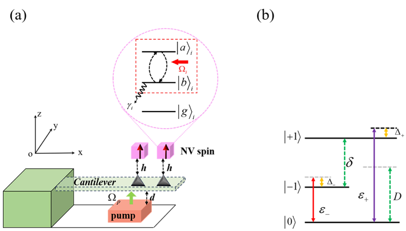
Figure B1: Two magnet tips are placed at the end of the silicon cantilever. The spring constant of the cantilever is modified by the electric field from the capacitor plate. Two microwave fields polarized in the x direction (not shown in the picture) are applied to drive the NV centers between the state $\left|{{m}_{s}}=0\right\rangle$ and the states $\left|{{m}_{s}}=\pm 1\right\rangle$. (b) Level diagram of the driven NV center electronic ground state $\left|{{m}_{s}}=0,\pm 1\right\rangle$.

By utilizing the two color microwave frequencies ${{\omega}_{\pm}}$, we can realize the transition between the states $\left|0\right\rangle$ and $\left|\pm 1\right\rangle$. In the rotating frame with the microwave frequencies ${{\omega}_{\pm}}$, we obtain the Hamiltonian ${{H}_{NV}}=\sum\limits_{j=\pm 1}{-{{\Delta}_{j}}\left|j\right\rangle\left\langle j\right|+\left({{\varepsilon}_{j}}/2\right)\left(\left|0\right\rangle\left\langle j\right|+\left|j\right\rangle\left\langle 0\right|\right)}$, where ${{\Delta}_{\pm}}\equiv\left|D-{{\omega}_{\pm}}\pm\delta/2\right|$ and ${{\varepsilon}_{\pm}}\equiv{{g}_{e}}{{\mu}_{B}}B_{0}^{\pm}/\sqrt{2}$ with the microwave classical fields $B_{x}^{\pm}(t)=B_{0}^{\pm}\cos({{\omega}_{\pm}}t+{{\phi}_{\pm}})$ polarized in the $x$ direction. In the following analysis, we take ${{\Delta}_{\pm}}=\Delta$ and ${{\varepsilon}_{\pm}}=\varepsilon$ for simplicity. The Hamiltonian for the nanomechanical resonator with a modulated spring is ${{H}_{mec}}=p_{z}^{2}/2M+\frac{1}{2}k(t){{z}^{2}}$, where ${{p}_{z}}$ and $z$ are the $\text{cantilever }\!\!^{\prime}\!\!\text{ s}$ momentum and displacement operators, with effective mass $M$ and fundamental frequency ${{\omega}_{m}}$. Expressing the momentum operator ${{p}_{z}}$ and the displacement operator $z$ with the oscillator $a$ of the fundamental oscillating mode and the zero field fluctuation ${{z}_{zpf}}=\sqrt{\hbar/2M{{\omega}_{m}}}$, i.e., ${{p}_{z}}=-i\sqrt{M\hbar{{\omega}_{m}}/2}(a-{{a}^{\dagger}})$ and $z={{z}_{zpf}}(a+{{a}^{\dagger}})$.

The Hamiltonian for describing the magnetic interaction between the NV spin and the cantilever vibrating mode can be written as ${{H}_{\operatorname{int}}}\equiv{{g}_{e}}{{\mu}_{B}}{{G}_{m}}z{{S}_{z}}$, with ${{G}_{m}}$ the magnetic field gradient. We switch to the dressed state basis $\left|b\right\rangle=1/\sqrt{2}\left(\left|+1\right\rangle-\left|-1\right\rangle\right)$, $\left|g\right\rangle=\cos\theta\left|0\right\rangle-\sin\theta\left|h\right\rangle$, $\left|a\right\rangle=\cos\theta\left|h\right\rangle+\sin\theta\left|0\right\rangle$, with $\left|h\right\rangle=1/\sqrt{2}\left(\left|+1\right\rangle+\left|-1\right\rangle\right)$ and $\tan(2\theta)=-\sqrt{2}\Omega/\Delta$. The lowest energy level $\left|g\right\rangle$ is a stable ground state, which can be treated as an effective continuum outside of the submanifold $\left|a\right\rangle$ and $\left|b\right\rangle$. Furthermore, we assume the transition frequency between the dressed states $\left|a\right\rangle$ and $\left|b\right\rangle$ is almost same as the oscillator frequency, i.e., ${{\omega}_{ab}}\sim{{\omega}_{m}}$. This system can be described as

$${{H}_{tot}} \simeq{{\delta}_{m}}{{a}^{\dagger}}a-\frac{{{\Omega}_{p}}}{2}\left({{a}^{2}}+{{a}^{\dagger 2}}\right)$$

$$\quad+\sum\limits_{i=1,2}\left[{{g}_{i}}\left({{a}^{\dagger}}\sigma_{i}^{-}+a\sigma_{i}^{\dagger}\right)+\frac{{{\delta}_{dg}}}{2}\sigma_{z}^{i}\right]$$ (11)

where the coefficients are ${{\delta}_{m}}={{\omega}_{m}}-{{\omega}_{p}}$, ${{\delta}_{ab}}={{\omega}_{ab}}-{{\omega}_{p}}$, $g={{g}_{e}}{{\mu}_{B}}{{G}_{m}}{{z}_{zpf}}\sin\theta$, $\sigma_{z}^{i}\equiv{{\left|a\right\rangle}_{i}}\left\langle a\right|-{{\left|b\right\rangle}_{i}}\left\langle b\right|$, $\sigma_{i}^{+}\equiv{{\left|a\right\rangle}_{i}}\left\langle b\right|$ and $\sigma_{i}^{-}\equiv{{\left|b\right\rangle}_{i}}\left\langle a\right|$. Therefore, it is obvious that the single NV can be seen as the two-level emitter. By applying another classical field to drive the two spins (with amplitude $\Omega$), the driving Hamiltonian can be obtained as ${{H}_{dri}}=\Omega(\sigma_{x}^{1}\text{+}\sigma_{x}^{2})$. Thus, the total Hamiltonian of our system can be rewritten as

$${{H}_{TO}}\simeq{{H}_{tot}}+{{H}_{dri}}.$$ (12)

Considering the Hamiltonian  (12), we can diagonalize the mechanical part of ${{H}_{TO}}$ by the unitary transmission ${{U}_{s}}(r)=\exp\left[r({{a}^{2}}-{{a}^{\dagger 2}})/2\right]$, where the squeezing parameter $r$ is defined via the relation $\tanh 2r={{\Omega}_{p}}/{{\delta}_{m}}$. Then, the total Hamiltonian  (12) in this squeezed frame can be obtained as

$$H_{TO} =H_{Rabi}^{S}+H_{sq}$$ (13)

$$H_{Rabi}^{S} ={{\Delta}_{m}}a_{s}^{\dagger}{{a}_{s}}+\sum\limits_{i=1,2}\left[{{g}_{eff,i}}({{a}_{s}}+a_{s}^{\dagger})(\sigma_{i}^{\dagger}+\sigma_{i}^{-})\right.$$

$$\quad+\left.\frac{{{\delta}_{dg}}}{2}\sigma_{z}^{i}\right]+{{H}_{dri}}$$

$$H_{sq} =\sum_{i=1,2}\frac{g_{i}e^{-r}}{2}(a_{s}-a_{s}^{\dagger})(\sigma_{i}^{\dagger}-\sigma_{i}^{-}).$$

Here, ${{g}_{eff,i}}={{g}_{i}}{{e}^{r}}/2$. Because the item ${{e}^{-r}}$ decreases to zero as the squeezing parameter $r$ increases, the Hamiltonian ${{H}_{sq}}$ can be ignored.

Considering ${{\delta}_{dg}}=0$ and ${{g}_{eff,1}}={{g}_{eff,2}}={{g}_{eff}}$, the Rabi Hamiltonian $H_{Rabi}^{S}$ can be reduced using the Schrieffer-Wolff transformation $H_{Rabi}^{eff}={{e}^{S}}H_{Rabi}^{S}{{e}^{-S}}$ where $S=\chi(a_{s}^{\dagger}-{{a}_{s}})(\sigma_{x}^{1}+\sigma_{x}^{2})$ and $\chi={{g}_{eff}}/{{\Delta}_{m}}$. Noted that the parameter $\chi$ is much smaller than one, indicating that it satisfies the Lamb-Dicke condition $\chi\ll 1$. The effective Hamiltonian is given by

$$H_{RT}^{eff}={{\Delta}_{m}}a_{s}^{\dagger}{{a}_{s}}-\xi{{\left(\sigma_{x}^{1}+\sigma_{x}^{2}\right)}^{2}}+\Omega(\sigma_{x}^{1}+\sigma_{x}^{2}).$$ (14)

where $\xi=g_{eff}^{2}/{{\Delta}_{m}}$. Owing to the operator ${{a}_{s}}$ is decoupled from the two-level emitter, we can only retain the second and third terms in Eq. (13). Especially, the second term is the typical Ising type interaction Hamiltonian ${{H}_{Ising}}=-\xi{{\left(\sigma_{x}^{1}+\sigma_{x}^{2}\right)}^{2}}$. Therefore, we rewritten the Hamiltonian Eq. (14) as

$${H}_{eff}=-\xi{{(\sigma_{x}^{1}+\sigma_{x}^{2})}^{2}}+\Omega(\sigma_{x}^{1}+\sigma_{x}^{2}).$$ (15)

In this scenario, the effective spin-spin interaction of the two NVs is obtained, and the phonon is only virtually excited. Taking the effective dissipation $\kappa_{a}^{s}$ and the decaying rate of spin $\gamma_{NV}^{i}$ into consideration, we have the master equation as follow:

$$\frac{d\rho}{dt}=-i\left[H_{Rabi}^{S},\rho\right]+\kappa_{a}^{S}D[a]\rho+\sum\limits_{i=1,2}{\gamma_{NV}^{i}D}[{\sigma}_{i}^{-}]\rho,$$ (16a)

$$\frac{d\rho}{dt}=-i\left[H_{eff},\rho\right]+\sum\limits_{i=1,2}{\gamma_{NV}^{i}D}[{\sigma}_{i}^{-}]\rho.$$ (16b)

where $D(O)\rho=O\rho{{O}^{\dagger}}-\frac{1}{2}\rho{{O}^{\dagger}}O-\frac{1}{2}{{O}^{\dagger}}O\rho$ is the Lindblad operator. Then we can make numerical simulations on the dynamical process according to Eq. (16). Figure B2 displays the concurrence $C$ for the case of two NV spins varying with the evolution time by respectively solving the two subequations in Eq. (16). We can obviously find that our approximation is reasonable.

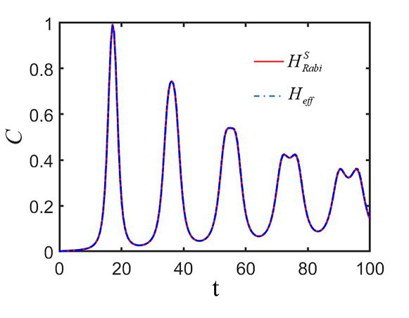
Figure B2: The concurrence evolution of the two spins system by respectively solving the two subequations of Eq. (16). The initial state of the system is $\left|0\right\rangle\left|aa\right\rangle$ and $\left|aa\right\rangle$ for Eq. (16)(a) and Eq. (16)(b), respectively. The left parameters are ${{\delta}_{dg}}=0$, $\kappa_{a}^{S}=\gamma_{NV}^{i}=\gamma$, $\Omega/\gamma=0.3$, $\xi/\gamma=0.0006$, ${{\Delta}_{m}}/\gamma=40$ and ${{g}_{eff}}=\sqrt{\xi{{\Delta}_{m}}}$.

Appendix C Non-Hermitian perturbation theory in Ising type interaction model

According to Eq. (15), The Hamiltonian for a single non-Hermitian qubit (or spin) reads as

$$H_{0}=-\frac{i\gamma_{j}}{2}\left|b\right\rangle_{j}\left\langle b\right|+\Omega\left(\left|a\right\rangle_{j}\left\langle b\right|+\left|b\right\rangle_{j}\left\langle a\right|\right),$$ (17)

$$H_{Ising,j}=-\xi\left(\left|a\right\rangle_{j}\left\langle b\right|+\left|b\right\rangle_{j}\left\langle a\right|\right)^{2},$$

with eigenvalues

$${{\lambda}_{j,\pm}}=\frac{1}{4}\left(-i\gamma-4\xi\pm\sqrt{16{{\Omega}^{2}}-{{\gamma}^{2}}}\right).$$ (18)

The eigenstates in this single-qubit Hilbert space $H$ are given by

$$\left|\psi_{j,-}\right\rangle =\frac{1}{4\sqrt{2}\Omega}\begin{pmatrix}i\gamma-\sqrt{16\Omega^{2}-\gamma^{2}}\\ 4\Omega\end{pmatrix},$$ (19)

$$\left|\psi_{j,+}\right\rangle =\frac{1}{4\sqrt{2}\Omega}\begin{pmatrix}i\gamma+\sqrt{16\Omega^{2}-\gamma^{2}}\\ 4\Omega\end{pmatrix}.$$

It is easy to find that both the eigenvalues and eigenstates combine at the same critical point, i.e., EP, at $\eta\equiv\sqrt{16{{\Omega}^{2}}-{{\gamma}^{2}}}=0$. And the above states are normalized (i.e., $\left\langle{{\psi}_{j,-(+)}}|{{\psi}_{j,-(+)}}\right\rangle=1$) but not orthogonal (i.e., $\left\langle{{\psi}_{j,-}}|{{\psi}_{j,+}}\right\rangle\neq 0$).

The non-Hermiticity of $H$ is the mean reason for the non-orthogonality, in order to better address the importance of non-Hermiticity, we extend the state basis to include states in the dual Hilbert space ${{H}^{*}}$. The Hamiltonian in the dual space ${{H}^{*}}$ is just the Hermitian conjugate of ${{H}_{j}}$ in Eq. (17). i.e., ${{\overline{H}}_{j}}=H_{j}^{\dagger}$, with the eigenvalues ${{\overline{\lambda}}_{\pm}}=\frac{1}{4}\left(i\gamma-4\xi\pm\sqrt{16{{\Omega}^{2}}-{{\gamma}^{2}}}\right)$ and the corresponding eigenstates

$$\left|\overline{\psi}_{j,-}\right\rangle =\frac{1}{4\sqrt{2}\Omega}\begin{pmatrix}-i\gamma-\sqrt{16\Omega^{2}-\gamma^{2}}\\ 4\Omega\end{pmatrix},$$ (20)

$$\left|\overline{\psi}_{j,+}\right\rangle =\frac{1}{4\sqrt{2}\Omega}\begin{pmatrix}-i\gamma+\sqrt{16\Omega^{2}-\gamma^{2}}\\ 4\Omega\end{pmatrix}.$$

To describe the two coupled non-Hermitian qubit in the absence of Ising type interaction, we construct the eigenstates and eigenvalues of the Hamiltonian ${{H}_{0}}$ and its Hermitian conjugate ${{\overline{H}}_{0}}=H_{0}^{\dagger}$. Focused on the $\mathcal{P}\mathcal{T}$-symmetric region, i.e., $\Omega>{{\Omega}_{\text{EP4}}}$, that is, $\eta>0$.

The first two eigenvalues of ${{H}_{0}}$ are given by

$$\lambda_{--} =2\lambda_{j,-}=\frac{1}{2}\left(-i\gamma-4\xi-\eta\right),$$ (21)

$$\lambda_{++} =2\lambda_{j,+}=\frac{1}{2}\left(-i\gamma-4\xi+\eta\right).$$

and the corresponding eigenvalues in the two-qubit Hilbert space are the product states of the eigenstates of the two qubits:

$$\left|\psi_{--}\right\rangle =\left|\psi_{1,-}\right\rangle\left|\psi_{2,-}\right\rangle=\frac{1}{32\Omega^{2}}\begin{pmatrix}-(\gamma+i\eta)^{2}\\ 4\Omega(i\gamma-\eta)\\ 4\Omega(i\gamma-\eta)\\ 16\Omega^{2}\end{pmatrix},$$ (22)

$$\left|\psi_{++}\right\rangle =\left|\psi_{1,+}\right\rangle\left|\psi_{2,+}\right\rangle=\frac{1}{32\Omega^{2}}\begin{pmatrix}(i\gamma+\eta)^{2}\\ 4\Omega(i\gamma+\eta)\\ 4\Omega(i\gamma+\eta)\\ 16\Omega^{2}\end{pmatrix}.$$

As for the dual space, the eigenvalues of ${{\overline{H}}_{0}}$ become

$$\overline{\lambda}_{--} =2\overline{\lambda}_{j,-}=\frac{1}{2}\left(i\gamma-4\xi-\eta\right),$$ (23)

$$\overline{\lambda}_{++} =2\overline{\lambda}_{j,+}=\frac{1}{2}\left(i\gamma-4\xi+\eta\right),$$

with the corresponding eigenstates are

$$\left|\overline{\psi}_{--}\right\rangle =\left|\overline{\psi}_{1,-}\right\rangle\left|\overline{\psi}_{2,-}\right\rangle=\frac{1}{32\Omega^{2}}\begin{pmatrix}-(\gamma-i\eta)^{2}\\ -4\Omega(i\gamma+\eta)\\ -4\Omega(i\gamma+\eta)\\ 16\Omega^{2}\end{pmatrix},$$ (24)

$$\left|\overline{\psi}_{++}\right\rangle =\left|\overline{\psi}_{1,+}\right\rangle\left|\overline{\psi}_{2,+}\right\rangle=\frac{1}{32\Omega^{2}}\begin{pmatrix}-(\gamma+i\eta)^{2}\\ -4\Omega(-i\gamma+\eta)\\ -4\Omega(-i\gamma+\eta)\\ 16\Omega^{2}\end{pmatrix}.$$

The above four eigenstates can be normalized via using biorthogonality

$$\left|\widetilde{\psi}_{--}\right\rangle =\frac{\left|\psi_{--}\right\rangle}{\sqrt{\left\langle\overline{\psi}_{--}|\psi_{--}\right\rangle}}=\frac{1}{2\eta}\begin{pmatrix}-i\gamma+\eta\\ -4\Omega\\ -4\Omega\\ i\gamma+\eta\end{pmatrix},$$ (25)

$$\left\langle\widetilde{\overline{\psi}}_{--}\right| =\frac{\left\langle\overline{\psi}_{--}\right|}{\sqrt{\left\langle\overline{\psi}_{--}|\psi_{--}\right\rangle}}$$

$$=\frac{1}{2\eta}\begin{pmatrix}-i\gamma+\eta&-4\Omega&-4\Omega&i\gamma+\eta\end{pmatrix},$$

$$\left|\widetilde{\psi}_{++}\right\rangle =\frac{\left|\psi_{++}\right\rangle}{\sqrt{\left\langle\overline{\psi}_{++}|\psi_{++}\right\rangle}}=\frac{1}{2\eta}\begin{pmatrix}i\gamma+\eta\\ 4\Omega\\ 4\Omega\\ -i\gamma+\eta\end{pmatrix},$$

$$\left\langle\widetilde{\overline{\psi}}_{++}\right| =\frac{\left\langle\overline{\psi}_{++}\right|}{\sqrt{\left\langle\overline{\psi}_{++}|\psi_{++}\right\rangle}}=\frac{1}{2\eta}\begin{pmatrix}i\gamma+\eta&4\Omega&4\Omega&-i\gamma+\eta\end{pmatrix}.$$

Here, $\left\langle{{\overline{\psi}}_{j}}\right|(j=+,-)$ are the Hermitian conjugates of $\left|{{\overline{\psi}}_{j}}\right\rangle$ in the dual space.

The other two eigenvalues of ${{H}_{0}}$ are degenerate and given by

$${{\lambda}_{-+}}={{\lambda}_{+-}}={{\lambda}_{j,-}}+{{\lambda}_{j,+}}=-\frac{i\gamma}{2}-2\xi,$$ (26)

with the corresponding eigenstates

$$\left|\psi_{-+}\right\rangle =\left|\psi_{1,-}\right\rangle\left|\psi_{2,+}\right\rangle=\frac{1}{8\Omega}\begin{pmatrix}-4\Omega\\ i\gamma-\eta\\ i\gamma+\eta\\ 4\Omega\end{pmatrix},$$ (27)

$$\left|\psi_{+-}\right\rangle =\left|\psi_{1,+}\right\rangle\left|\psi_{2,-}\right\rangle=\frac{1}{8\Omega}\begin{pmatrix}-4\Omega\\ i\gamma+\eta\\ i\gamma-\eta\\ 4\Omega\end{pmatrix}.$$

For the eigenvalues and eigenstates of ${{\overline{H}}_{0}}$ in the dual space are given by,

$${{\overline{\lambda}}_{-+}}={{\overline{\lambda}}_{+-}}={{\overline{\lambda}}_{j,-}}+{{\overline{\lambda}}_{j,+}}=\frac{i\gamma}{2}-2\xi.$$ (28)

And the corresponding eigenstates

$$\left|\overline{\psi}_{-+}\right\rangle =\left|\overline{\psi}_{1,-}\right\rangle\left|\overline{\psi}_{2,+}\right\rangle=\frac{1}{8\Omega}\begin{pmatrix}-4\Omega\\ -i\gamma-\eta\\ -i\gamma+\eta\\ 4\Omega\end{pmatrix},$$ (29)

$$\left|\overline{\psi}_{+-}\right\rangle =\left|\overline{\psi}_{1,+}\right\rangle\left|\overline{\psi}_{2,-}\right\rangle=\frac{1}{8\Omega}\begin{pmatrix}-4\Omega\\ -i\gamma+\eta\\ -i\gamma-\eta\\ 4\Omega\end{pmatrix}.$$

Similarly, we can build the normalized and unperturbed biorthogonal eigenstates in the degenerate subspace.

$$\left|\widetilde{\psi}_{-+}\right\rangle =\frac{\left|\psi_{-+}\right\rangle}{\sqrt{\left\langle\overline{\psi}_{-+}|\psi_{-+}\right\rangle}}=\frac{1}{2\eta}\begin{pmatrix}-4\Omega\\ i\gamma-\eta\\ i\gamma+\eta\\ 4\Omega\end{pmatrix},$$ (30)

$$\left\langle\widetilde{\overline{\psi}}_{-+}\right| =\frac{\left\langle\overline{\psi}_{-+}\right|}{\sqrt{\left\langle\overline{\psi}_{-+}|\psi_{-+}\right\rangle}}=\frac{1}{2\eta}\begin{pmatrix}-4\Omega&i\gamma-\eta&i\gamma+\eta&4\Omega\end{pmatrix},$$

$$\left|\widetilde{\psi}_{+-}\right\rangle =\frac{\left|\psi_{+-}\right\rangle}{\sqrt{\left\langle\overline{\psi}_{+-}|\psi_{+-}\right\rangle}}=\frac{1}{2\eta}\begin{pmatrix}-4\Omega\\ i\gamma+\eta\\ i\gamma-\eta\\ 4\Omega\end{pmatrix},$$

$$\left\langle\widetilde{\overline{\psi}}_{+-}\right| =\frac{\left\langle\overline{\psi}_{+-}\right|}{\sqrt{\left\langle\overline{\psi}_{+-}|\psi_{+-}\right\rangle}}=\frac{1}{2\eta}\begin{pmatrix}-4\Omega&i\gamma+\eta&i\gamma-\eta&4\Omega\end{pmatrix}.$$

C.1 $\mathcal{P}\mathcal{T}$-symmetry-broken phase, $\eta<0$

For the $\mathcal{P}\mathcal{T}$-symmetry-broken phase, i.e., $\eta<0$, we can also present the conventionally normalized eigenvectors $\left|{{\psi}_{i}}\right\rangle$ in the broken phase, namely

$$\left|{\psi}_{--}\right\rangle=\frac{1}{32{\Omega}^{2}}\begin{pmatrix}{(i\gamma+\eta)^{2}}\\ 4\Omega(i\gamma+\eta)\\ 4\Omega(i\gamma+\eta)\\ 16{\Omega}^{2}\end{pmatrix},$$ (31)

$$\left|{\psi}_{++}\right\rangle=\frac{1}{32{\Omega}^{2}}\begin{pmatrix}{-(\gamma+i\eta)^{2}}\\ 4\Omega(i\gamma-\eta)\\ 4\Omega(i\gamma-\eta)\\ 16{\Omega}^{2}\end{pmatrix},$$

$$\left|{\psi}_{-+}\right\rangle=\frac{1}{8\Omega}\begin{pmatrix}-4\Omega\\ i\gamma+\eta\\ i\gamma-\eta\\ 4\Omega\end{pmatrix},\left|{\psi}_{+-}\right\rangle=\frac{1}{8\Omega}\begin{pmatrix}-4\Omega\\ i\gamma-\eta\\ i\gamma+\eta\\ 4\Omega\end{pmatrix},$$

with corresponding eigenvalues calculated by ${{\lambda}_{--}}=2{{\lambda}_{j,-}}=\frac{1}{2}\left(-i\gamma-4\xi+\eta\right),{{\lambda}_{++}}=2{{\lambda}_{j,+}}=\frac{1}{2}\left(-i\gamma-4\xi-\eta\right)$ and ${{\lambda}_{-+}}={{\lambda}_{+-}}=-\frac{i\gamma}{2}-2\xi$, respectively.

C.2 First-order degenerate and non-degenerate perturbation theory with Ising type interaction

The perturbation matrix in the subspace spanned by $\left\{\left|{{\widetilde{\psi}}_{+-}}\right\rangle,\left|{{\widetilde{\psi}}_{-+}}\right\rangle\right\}$ and their adjoint states $\left\{\left\langle{{\widetilde{\overline{\psi}}}_{+-}}\right|,\left\langle{{\widetilde{\overline{\psi}}}_{-+}}\right|\right\}$. This matrix can be obtained as

$$\left[H_{\text{int}}\right] =\begin{pmatrix}\left\langle\widetilde{\overline{\psi}}_{+-}\middle|H_{\text{int}}\middle|\widetilde{\psi}_{+-}\right\rangle&\left\langle\widetilde{\overline{\psi}}_{-+}\middle|H_{\text{int}}\middle|\widetilde{\psi}_{+-}\right\rangle\\ \left\langle\widetilde{\overline{\psi}}_{-+}\middle|H_{\text{int}}\middle|\widetilde{\psi}_{+-}\right\rangle&\left\langle\widetilde{\overline{\psi}}_{-+}\middle|H_{\text{int}}\middle|\widetilde{\psi}_{-+}\right\rangle\end{pmatrix}$$ (32)

$$=\begin{pmatrix}-\frac{J\gamma^{2}}{\eta^{2}}&-\frac{J\gamma^{2}}{\eta^{2}}\\ -\frac{J\gamma^{2}}{\eta^{2}}&-\frac{J\gamma^{2}}{\eta^{2}}\end{pmatrix}.$$

Here, $J=-2\xi$. Noted that ${{H}_{\operatorname{int}}}$ is Hermitian and this submatrix is real with eigenvalues 0 and $-\frac{2J{{\gamma}^{2}}}{{{\eta}^{2}}}$. The eigenstates read as $\left(\left|{{\psi}_{-+}}\right\rangle\mp\left|{{\psi}_{+-}}\right\rangle\right)/\sqrt{2}$, which means that we can choose a new basis for the degenerate subspace, specifically,

$$\left|\widetilde{\psi}_{1}\right\rangle =\frac{1}{\sqrt{2}}\left(\left|\widetilde{\psi}_{-+}\right\rangle-\left|\widetilde{\psi}_{+-}\right\rangle\right)=\frac{1}{\sqrt{2}}\begin{pmatrix}0\\ -1\\ 1\\ 0\end{pmatrix},$$ (33)

$$\left|\widetilde{\psi}_{2}\right\rangle =\frac{1}{\sqrt{2}}\left(\left|\widetilde{\psi}_{-+}\right\rangle+\left|\widetilde{\psi}_{+-}\right\rangle\right)=\frac{1}{\sqrt{2}\eta}\begin{pmatrix}-4\Omega\\ i\gamma\\ i\gamma\\ 4\Omega\end{pmatrix},$$

$$\left|\widetilde{\overline{\psi}}_{1}\right\rangle =\frac{1}{\sqrt{2}}\left(\left|\widetilde{\overline{\psi}}_{-+}\right\rangle-\left|\widetilde{\overline{\psi}}_{+-}\right\rangle\right)=\frac{1}{\sqrt{2}}\begin{pmatrix}0\\ -1\\ 1\\ 0\end{pmatrix},$$

$$\left|\widetilde{\overline{\psi}}_{2}\right\rangle =\frac{1}{\sqrt{2}}\left(\left|\widetilde{\overline{\psi}}_{-+}\right\rangle+\left|\widetilde{\overline{\psi}}_{+-}\right\rangle\right)=\frac{1}{\sqrt{2}\eta}\begin{pmatrix}-4\Omega\\ -i\gamma\\ -i\gamma\\ 4\Omega\end{pmatrix}.$$

Noted that this type of interaction Hamiltonian ${{H}_{\operatorname{int}}}$ is diagonal and the state $\left|{{\widetilde{\psi}}_{1}}\right\rangle$is equal to $\left|{{\widetilde{\overline{\psi}}}_{1}}\right\rangle$. The corresponding eigenvalues are given by

$${{\lambda}_{1}}={{\lambda}_{-+}},{{\overline{\lambda}}_{1}}={{\overline{\lambda}}_{-+}},{{\lambda}_{2}}={{\lambda}_{+-}},{{\overline{\lambda}}_{2}}={{\overline{\lambda}}_{+-}}.$$ (34)

It is easy to find that $\left|{{\widetilde{\psi}}_{1}}\right\rangle=\left|{{\widetilde{\overline{\psi}}}_{1}}\right\rangle$. Applying to the first-order non-degenerate perturbation theory to our system of two weakly coupled non-Hermitian spins. The perturbed eigenvalues are given by

$$\Lambda_{1} =\lambda_{1}+0=-\frac{i\gamma}{2}-2\xi,$$ (35)

$$\overline{\Lambda}_{1} =\overline{\lambda}_{1}+0=\frac{i\gamma}{2}-2\xi,$$

$$\Lambda_{2} =\lambda_{2}-\frac{2J\gamma^{2}}{\eta^{2}}=-\frac{i\gamma}{2}-2\xi-\frac{2J\gamma^{2}}{\eta^{2}},$$

$$\overline{\Lambda}_{2} =\overline{\lambda}_{2}-\frac{2J\gamma^{2}}{\eta^{2}}=\frac{i\gamma}{2}-2\xi-\frac{2J\gamma^{2}}{\eta^{2}}.$$

Finding that the given interaction Hamiltonian is already diagonal in the basis $\left\{\left|{{\widetilde{\psi}}_{1}}\right\rangle,\left|{{\widetilde{\psi}}_{2}}\right\rangle\right\}$ of the Hilbert space and $\left\{\left|{{\widetilde{\overline{\psi}}}_{1}}\right\rangle,\left|{{\widetilde{\overline{\psi}}}_{2}}\right\rangle\right\}$ of the dual space. Therefore, we need to consider the first-order unperturbed eigenstates of the non-degenerate subspace.

$$\left|{{\Psi}_{1}}\right\rangle=\left|{{\overline{\Psi}}_{1}}\right\rangle =\left|{{\widetilde{\psi}}_{1}}\right\rangle+\frac{\left\langle{{\widetilde{\overline{\psi}}}_{--}}\right|{{H}_{\operatorname{int}}}\left|{{\widetilde{\psi}}_{1}}\right\rangle}{{{\lambda}_{1}}-{{\lambda}_{--}}}\left|{{\widetilde{\psi}}_{--}}\right\rangle$$ (36)

$$+\frac{\left\langle{{\widetilde{\overline{\psi}}}_{++}}\right|{{H}_{\operatorname{int}}}\left|{{\widetilde{\psi}}_{1}}\right\rangle}{{{\lambda}_{1}}-{{\lambda}_{++}}}\left|{{\widetilde{\psi}}_{++}}\right\rangle$$

$$=\frac{1}{\sqrt{2}}\left(\begin{matrix}0\\ -1\\ 1\\ 0\\ \end{matrix}\right),$$

$$\left|{{\Psi}_{2}}\right\rangle =\left|{{\widetilde{\psi}}_{2}}\right\rangle+\frac{\left\langle{{\widetilde{\overline{\psi}}}_{--}}\right|{{H}_{\operatorname{int}}}\left|{{\widetilde{\psi}}_{2}}\right\rangle}{{{\lambda}_{2}}-{{\lambda}_{--}}}\left|{{\widetilde{\psi}}_{--}}\right\rangle$$ (37)

$$+\frac{\left\langle{{\widetilde{\overline{\psi}}}_{++}}\right|{{H}_{\operatorname{int}}}\left|{{\widetilde{\psi}}_{2}}\right\rangle}{{{\lambda}_{2}}-{{\lambda}_{++}}}\left|{{\widetilde{\psi}}_{++}}\right\rangle$$

$$=\frac{1}{\sqrt{2}{{\eta}^{3}}}\left(\begin{matrix}-4\Omega{{\eta}^{2}}-i16\gamma J\Omega\\ i\gamma{{\eta}^{2}}\\ i\gamma{{\eta}^{2}}\\ 4\Omega{{\eta}^{2}}-i16\gamma J\Omega\\ \end{matrix}\right),$$

$$\left|{{\overline{\Psi}}_{2}}\right\rangle =\left|{{\widetilde{\overline{\psi}}}_{2}}\right\rangle+\frac{\left\langle{{\widetilde{\psi}}_{--}}\right|{{H}_{\operatorname{int}}}\left|{{\widetilde{\overline{\psi}}}_{2}}\right\rangle}{{{\lambda}_{2}}-{{\lambda}_{--}}}\left|{{\widetilde{\overline{\psi}}}_{--}}\right\rangle$$ (38)

$$+\frac{\left\langle{{\widetilde{\psi}}_{++}}\right|{{H}_{\operatorname{int}}}\left|{{\widetilde{\overline{\psi}}}_{2}}\right\rangle}{{{\lambda}_{2}}-{{\lambda}_{++}}}\left|{{\widetilde{\overline{\psi}}}_{++}}\right\rangle$$

$$=\frac{1}{\sqrt{2}{{\eta}^{3}}}\left(\begin{matrix}-4\Omega{{\eta}^{2}}+i16\gamma J\Omega\\ -i\gamma{{\eta}^{2}}\\ -i\gamma{{\eta}^{2}}\\ 4\Omega{{\eta}^{2}}+i16\gamma J\Omega\\ \end{matrix}\right).$$

The perturbed eigenvalues are given by

$$\left|\Psi_{++}\right\rangle =\left|\widetilde{\psi}_{++}\right\rangle+\frac{\left\langle\widetilde{\overline{\psi}}_{--}\middle|H_{\text{int}}\middle|\widetilde{\psi}_{++}\right\rangle}{{\lambda_{++}-\lambda_{--}}}\left|\widetilde{\psi}_{--}\right\rangle+\frac{\left\langle\widetilde{\overline{\psi}}_{1}\middle|H_{\text{int}}\middle|\widetilde{\psi}_{++}\right\rangle}{{\lambda_{++}-\lambda_{1}}}\left|\widetilde{\psi}_{1}\right\rangle+\frac{\left\langle\widetilde{\overline{\psi}}_{2}\middle|H_{\text{int}}\middle|\widetilde{\psi}_{++}\right\rangle}{{\lambda_{++}-\lambda_{2}}}\left|\widetilde{\psi}_{2}\right\rangle$$ (39)

$$=\frac{1}{2\eta}\begin{pmatrix}i\gamma+\eta\\ 4\Omega\\ 4\Omega\\ -i\gamma+\eta\end{pmatrix}-\frac{8J\Omega^{2}}{{\eta^{4}}}\begin{pmatrix}-i\gamma+\eta\\ -4\Omega\\ -4\Omega\\ i\gamma+\eta\end{pmatrix}+\frac{8i\gamma J\Omega}{{\eta^{4}}}\begin{pmatrix}-4\Omega\\ i\gamma\\ i\gamma\\ 4\Omega\end{pmatrix},$$

$$\left|\Psi_{--}\right\rangle =\left|\widetilde{\psi}_{--}\right\rangle+\frac{\left\langle\widetilde{\overline{\psi}}_{++}\middle|H_{\text{int}}\middle|\widetilde{\psi}_{--}\right\rangle}{{\lambda_{--}-\lambda_{++}}}\left|\widetilde{\psi}_{++}\right\rangle+\frac{\left\langle\widetilde{\overline{\psi}}_{1}\middle|H_{\text{int}}\middle|\widetilde{\psi}_{--}\right\rangle}{{\lambda_{--}-\lambda_{1}}}\left|\widetilde{\psi}_{1}\right\rangle+\frac{\left\langle\widetilde{\overline{\psi}}_{2}\middle|H_{\text{int}}\middle|\widetilde{\psi}_{--}\right\rangle}{{\lambda_{--}-\lambda_{2}}}\left|\widetilde{\psi}_{2}\right\rangle$$ (40)

$$=\frac{1}{2\eta}\begin{pmatrix}-i\gamma+\eta\\ -4\Omega\\ -4\Omega\\ i\gamma+\eta\end{pmatrix}+\frac{8J\Omega^{2}}{{\eta^{4}}}\begin{pmatrix}i\gamma+\eta\\ 4\Omega\\ 4\Omega\\ -i\gamma+\eta\end{pmatrix}+\frac{8i\gamma J\Omega}{{\eta^{4}}}\begin{pmatrix}-4\Omega\\ i\gamma\\ i\gamma\\ 4\Omega\end{pmatrix}.$$

The above perturbation theory gives the basis states, i.e., $\left|{{\psi}_{++}}\right\rangle,\left|{{\psi}_{--}}\right\rangle,\left|{{\psi}_{1}}\right\rangle,\left|{{\psi}_{2}}\right\rangle$ in the Hibert space $H$ as well as the corresponding adjoint states $\left|{{\overline{\psi}}_{++}}\right\rangle,\left|{{\overline{\psi}}_{--}}\right\rangle,\left|{{\overline{\psi}}_{1}}\right\rangle,\left|{{\overline{\psi}}_{2}}\right\rangle$ in the dual space ${{H}^{*}}$. It is worth to note that the above basis states are both normalized

$$\left\langle{{\overline{\psi}}_{1}}|{{\psi}_{1}}\right\rangle=1and\left\langle{{\overline{\psi}}_{i}}|{{\psi}_{i}}\right\rangle=1+O({{\xi}^{2}}),(i=++,--,2)$$ (41)

and orthogonal, namely

$$\left\langle{{\overline{\psi}}_{i}}|{{\psi}_{j}}\right\rangle=0+O({{\xi}^{2}}),(i,j=++,--,1,2)$$ (42)

Moreover, they also compose a complete basis

$$\left|{{\psi}_{++}}\right\rangle\left\langle{{\overline{\psi}}_{++}}\right| +\left|{{\psi}_{--}}\right\rangle\left\langle{{\overline{\psi}}_{--}}\right|$$ (43)

$$+\left|{{\psi}_{1}}\right\rangle\left\langle{{\overline{\psi}}_{1}}\right|+\left|{{\psi}_{2}}\right\rangle\left\langle{{\overline{\psi}}_{2}}\right|$$

$$=1+O({{\xi}^{2}}).$$

For the non-degenerate subspaces, the correction at the first order is determined by the expectation values of the interaction Hamiltonian using the unperturbed eigenstates

$$\Lambda_{--} =\lambda_{--}+\left\langle\widetilde{\overline{\psi}}_{--}\middle|H_{\text{int}}\middle|\widetilde{\psi}_{--}\right\rangle$$ (44)

$$=\frac{1}{2}\left(-i\gamma-4\xi-\eta\right)+\frac{16J\Omega^{2}}{{\eta^{2}}},$$

$$\Lambda_{++} =\lambda_{++}+\left\langle\widetilde{\overline{\psi}}_{++}\middle|H_{\text{int}}\middle|\widetilde{\psi}_{++}\right\rangle$$

$$=\frac{1}{2}\left(-i\gamma-4\xi+\eta\right)+\frac{16J\Omega^{2}}{{\eta^{2}}}.$$

C.3 Entanglement between two coupled non-Hermitian qubits

Given an initial state $\left|\psi(0)\right\rangle$, the time evolution of the state under an evolution operator $U={{e}^{-iHt}}$ can be obtained by

$$\left|\psi(t)\right\rangle =U\left|\psi(0)\right\rangle=\left\langle\overline{\Psi}_{++}\middle|\psi(0)\right\rangle e^{-it\Lambda_{++}}\left|\Psi_{++}\right\rangle\quad+\left\langle\overline{\Psi}_{--}\middle|\psi(0)\right\rangle e^{-it\Lambda_{--}}\left|\Psi_{--}\right\rangle$$ (45)

$$\quad+\left\langle\overline{\Psi}_{1}\middle|\psi(0)\right\rangle e^{-it\Lambda_{1}}\left|\Psi_{1}\right\rangle\quad+\left\langle\overline{\Psi}_{2}\middle|\psi(0)\right\rangle e^{-it\Lambda_{2}}\left|\Psi_{2}\right\rangle$$

$$=A_{1}e^{-it\Lambda_{++}}\left|\Psi_{++}\right\rangle+A_{2}e^{-it\Lambda_{--}}\left|\Psi_{--}\right\rangle\quad+A_{3}e^{-it\Lambda_{1}}\left|\Psi_{1}\right\rangle+A_{4}e^{-it\Lambda_{2}}\left|\Psi_{2}\right\rangle,$$

where

$$A_{1}=\frac{1}{2\eta}(i\gamma+\eta)-\frac{8J\Omega^{2}}{{\eta^{4}}}(-i\gamma+\eta)+\frac{8i\gamma J\Omega}{{\eta^{4}}}(-4\Omega),$$ (46)

$$A_{2}=\frac{1}{2\eta}(-i\gamma+\eta)+\frac{8J\Omega^{2}}{{\eta^{4}}}(i\gamma+\eta)+\frac{8i\gamma J\Omega}{{\eta^{4}}}(-4\Omega),$$

$$A_{3}=0,$$

$$A_{4}=\frac{1}{\sqrt{2}\eta^{3}}(-4\Omega\eta^{2}-i16\gamma J\Omega).$$

By projecting this two-qubit pure state onto the four maximally entangled Bell states, i.e., $\left|\psi\right\rangle=\sum\limits_{j}{{{c}_{j}}\left|{{e}_{j}}\right\rangle}$ with

$$\left|e_{1}\right\rangle=\frac{1}{\sqrt{2}}\left(\left|aa\right\rangle+\left|bb\right\rangle\right), \left|e_{2}\right\rangle=\frac{i}{\sqrt{2}}\left(\left|aa\right\rangle-\left|bb\right\rangle\right),$$ (47)

$$\left|e_{3}\right\rangle=\frac{1}{\sqrt{2}}\left(\left|ab\right\rangle+\left|ba\right\rangle\right), \left|e_{4}\right\rangle=\frac{1}{\sqrt{2}}\left(\left|ab\right\rangle-\left|ba\right\rangle\right),$$

The concurrence as an entanglement of the two coupled qubit can be written as

$$C=\frac{\left|\left\langle{{\psi}^{*}}|\psi\right\rangle\right|}{{{\left|\left|\psi(t)\right\rangle\right|}^{2}}}=\frac{2\left|\alpha\delta-\beta\varsigma\right|}{{{\left|\alpha\right|}^{2}}+{{\left|\beta\right|}^{2}}+{{\left|\varsigma\right|}^{2}}+{{\left|\delta\right|}^{2}}}.$$ (48)

The results show that the analytical simulation by utilizing the perturbation theory assuming the weak qubit coupling up to first order in the $\mathcal{P}\mathcal{T}$-symmetric phase. As an example, by choosing the weak Ising type interaction for $\xi/\gamma=0.0006$, the maximum entanglement ($C=1$) will occur at the specific time ${{T}^{*}}=17.17$ for a given value of $\Omega/\gamma=0.3$ in the PTS, as shown in Figure C1. Importantly, the analytical result shows good agreement with the numerical calculation. In particular, the maximum degree of entanglement can be obtained at a shorter timescale.

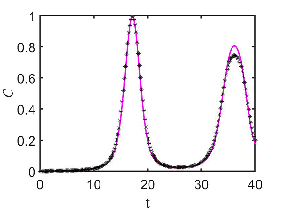
Figure C1: Comparison of the calculated concurrence evolution $C$ from the first-order non-Hermitian perturbation theory (the solid lines see Eq. (48)) and the fully numerical solution (asterisk on solid lines) at values in the $\mathcal{P}\mathcal{T}$-symmetric phase: $\Omega/\gamma=0.3$ as an example. The initial state is $\left|\psi(0)\right\rangle=\left|aa\right\rangle$ and the coupling strength is $\xi/\gamma=0.0006$.

References

Bender and Boettcher (1998)Carl M. Bender and Stefan Boettcher, “Real Spectra in Non-Hermitian Hamiltonians Having Symmetry,” Phys. Rev. Lett. 80, 5243–5246 (1998).
Rüter et al. (2010)C. E. Rüter, K. G. Makris, R. El-Ganainy, D. N. Christodoulides, M. Segev, and D. Kip, “Observation of parity-time symmetry in optics,” Nat. Phys. 6, 192–195 (2010).
El-Ganainy et al. (2018)R. El-Ganainy, K. G. Makris, M. Khajavikhan, Z. H. Musslimani, S. Rotter, and D. N. Christodoulides, “Non-Hermitian physics and PT symmetry,” Nat. Phys. 14, 11–19 (2018).
Hodaei et al. (2017)H. Hodaei, A. U. Hassan, S. Wittek, H. Garcia-Gracia, R. El-Ganainy, D. N. Christodoulides, and M. Khajavikhan, “Enhanced sensitivity at higher-order exceptional points,” Nature 548, 187 (2017).
Zhu et al. (2018)Weiwei Zhu, Xinsheng Fang, Dongting Li, Yong Sun, Yong Li, Yun Jing, and Hong Chen, “Simultaneous Observation of a Topological Edge State and Exceptional Point in an Open and Non-Hermitian Acoustic System,” Phys. Rev. Lett. 121, 124501 (2018).
Liu et al. (2018)Tuo Liu, Xuefeng Zhu, Fei Chen, Shanjun Liang, and Jie Zhu, “Unidirectional Wave Vector Manipulation in Two-Dimensional Space with an All Passive Acoustic Parity-Time-Symmetric Metamaterials Crystal,” Phys. Rev. Lett. 120, 124502 (2018).
Yang et al. (2020)Y. Yang, Yi-Pu Wang, J. W. Rao, Y. S. Gui, B. M. Yao, W. Lu, and C.-M. Hu, “Unconventional Singularity in Anti-Parity-Time Symmetric Cavity Magnonics,” Phys. Rev. Lett. 125, 147202 (2020).
Wang et al. (2019)Yi-Pu Wang, J. W. Rao, Y. Yang, Peng-Chao Xu, Y. S. Gui, B. M. Yao, J. Q. You, and C.-M. Hu, “Nonreciprocity and Unidirectional Invisibility in Cavity Magnonics,” Phys. Rev. Lett. 123, 127202 (2019).
Bergholtz et al. (2021)Emil J. Bergholtz, Jan Carl Budich, and Flore K. Kunst, “Exceptional topology of non-Hermitian systems,” Rev. Mod. Phys. 93, 015005 (2021).
Özdemir et al. (2019)S. K. Özdemir, S. Rotter, F. Nori, and L. Yang, “Parity-time symmetry and exceptional points in photonics,” Nat. Mater. 18, 783–798 (2019).
Parto et al. (2021)M. Parto, Yzgn Liu, B. Bahari, M. Khajavikhan, and D. N. Christodoulides, “Non-Hermitian and topological photonics: optics at an exceptional point,” Nanophotonics 10, 403–423 (2021).
Miri and Alù (2019)M. A. Miri and A. Alù, “Exceptional points in optics and photonics,” Science 363, 42 (2019).
Peng et al. (2014a)B. Peng, S. K. Özdemir, F. C. Lei, F. Monifi, M. Gianfreda, G. L. Long, S. H. Fan, F. Nori, C. M. Bender, and L. Yang, “Parity-time-symmetric whispering-gallery microcavities,” Nat. Phys. 10, 394–398 (2014a).
Chang et al. (2014)L. Chang, X. S. Jiang, S. Y. Hua, C. Yang, J. M. Wen, L. Jiang, G. Y. Li, G. Z. Wang, and M. Xiao, “Parity-time symmetry and variable optical isolation in active-passive-coupled microresonators,” Nat. Photonics 8, 524–529 (2014).
Peng et al. (2014b)B. Peng, S. K. Özdemir, S. Rotter, H. Yilmaz, M. Liertzer, F. Monifi, C. M. Bender, F. Nori, and L. Yang, “Loss-induced suppression and revival of lasing,” Science 346, 328–332 (2014b).
Zhang et al. (2018)H. Zhang, F. Saif, Y. Jiao, and H. Jing, “Loss-induced transparency in optomechanics,” Opt. Express 26, 25199–25210 (2018).
Sun et al. (2014)Yong Sun, Wei Tan, Hong-qiang Li, Jensen Li, and Hong Chen, “Experimental Demonstration of a Coherent Perfect Absorber with PT Phase Transition,” Phys. Rev. Lett. 112, 143903 (2014).
Wang et al. (2021)C. Q. Wang, W. R. Sweeney, A. D. Stone, and L. Yang, “Coherent perfect absorption at an exceptional point,” Science 373, 1261 (2021).
Assawaworrarit and Fan (2020)S. Assawaworrarit and S. H. Fan, “Robust and efficient wireless power transfer using a switch-mode implementation of a nonlinear parity-time symmetric circuit,” Nat. Electron. 3, 273–279 (2020).
Assawaworrarit et al. (2017)S. Assawaworrarit, X. F. Yu, and S. H. Fan, “Robust wireless power transfer using a nonlinear parity-time-symmetric circuit,” Nature 546, 387 (2017).
Feng et al. (2014)L. Feng, Z. J. Wong, R. M. Ma, Y. Wang, and X. Zhang, “Single-mode laser by parity-time symmetry breaking,” Science 346, 972–975 (2014).
Wu et al. (2019)Y. Wu, W. Q. Liu, J. P. Geng, X. R. Song, X. Y. Ye, C. K. Duan, X. Rong, and J. F. Du, “Observation of parity-time symmetry breaking in a single-spin system,” Science 364, 878 (2019).
Naghiloo et al. (2019)M. Naghiloo, M. Abbasi, Y. N. Joglekar, and K. W. Murch, “Quantum state tomography across the exceptional point in a single dissipative qubit,” Nat. Phys. 15, 1232 (2019).
Xiao et al. (2020)L. Xiao, T. S. Deng, K. K. Wang, G. Y. Zhu, Z. Wang, W. Yi, and P. Xue, “Non-Hermitian bulk-boundary correspondence in quantum dynamics,” Nat. Phys. 16, 761 (2020).
Öztürk et al. (2021)F. E. Öztürk, T. Lappe, G. Hellmann, J. Schmitt, J. Klaers, F. Vewinger, J. Kroha, and M. Weitz, “Observation of a non-Hermitian phase transition in an optical quantum gas,” Science 372, 88 (2021).
Chen et al. (2021)Weijian Chen, Maryam Abbasi, Yogesh N. Joglekar, and Kater W. Murch, “Quantum Jumps in the Non-Hermitian Dynamics of a Superconducting Qubit,” Phys. Rev. Lett. 127, 140504 (2021).
Chen et al. (2022)Weijian Chen, Maryam Abbasi, Byung Ha, Serra Erdamar, Yogesh N. Joglekar, and Kater W. Murch, “Decoherence-Induced Exceptional Points in a Dissipative Superconducting Qubit,” Phys. Rev. Lett. 128, 110402 (2022).
Ding et al. (2021)Liangyu Ding, Kaiye Shi, Qiuxin Zhang, Danna Shen, Xiang Zhang, and Wei Zhang, “Experimental Determination of -Symmetric Exceptional Points in a Single Trapped Ion,” Phys. Rev. Lett. 126, 083604 (2021).
Cao et al. (2020)Wanxia Cao, Xingda Lu, Xin Meng, Jian Sun, Heng Shen, and Yanhong Xiao, “Reservoir-Mediated Quantum Correlations in Non-Hermitian Optical System,” Phys. Rev. Lett. 124, 030401 (2020).
Liang et al. (2023)Chao Liang, Yuanjiang Tang, An-Ning Xu, and Yong-Chun Liu, “Observation of Exceptional Points in Thermal Atomic Ensembles,” Phys. Rev. Lett. 130, 263601 (2023).
Li et al. (2019)J. M. Li, A. K. Harterg, J. Liu, L. de Melo, Y. N. Joglekar, and L. Luo, “Observation of parity-time symmetry breaking transitions in a dissipative Floquet system of ultracold atoms,” Nat. Commun. 10 (2019), 10.1038/s41467-019-08596-1.
Lee and Chan (2014)Tony E. Lee and Ching-Kit Chan, “Heralded Magnetism in Non-Hermitian Atomic Systems,” Phys. Rev. X 4, 041001 (2014).
Pick et al. (2019)A. Pick, S. Silberstein, N. Moiseyev, and N. Bar-Gill, “Robust mode conversion in NV centers using exceptional points,” Phys. Rev. Res. 1, 013015 (2019).
Huang et al. (2022)R. Huang, S. K. Özdemir, J. Q. Liao, F. Minganti, L. M. Kuang, F. Nori, and H. Jing, “Exceptional Photon Blockade: Engineering Photon Blockade with Chiral Exceptional Points,” Laser Photonics Rev. 16 (2022), 10.1002/lpor.202100430.
Zuo et al. (2022)Yunlan Zuo, Ran Huang, Le-Man Kuang, Xun-Wei Xu, and Hui Jing, “Loss-induced suppression, revival, and switch of photon blockade,” Phys. Rev. A 106, 043715 (2022).
Yuan et al. (2023)Zhong-Hui Yuan, Yong-Jian Chen, Jin-Xuan Han, Jin-Lei Wu, Wei-Qi Li, Yan Xia, Yong-Yuan Jiang, and Jie Song, “Periodic photon-magnon blockade in an optomagnonic system with chiral exceptional points,” Phys. Rev. B 108, 134409 (2023).
Liu et al. (2021)Wenquan Liu, Yang Wu, Chang-Kui Duan, Xing Rong, and Jiangfeng Du, “Dynamically Encircling an Exceptional Point in a Real Quantum System,” Phys. Rev. Lett. 126, 170506 (2021).
Gong et al. (2018)Zongping Gong, Yuto Ashida, Kohei Kawabata, Kazuaki Takasan, Sho Higashikawa, and Masahito Ueda, “Topological Phases of Non-Hermitian Systems,” Phys. Rev. X 8, 031079 (2018).
Xu et al. (2016)H. Xu, D. Mason, L. Y. Jiang, and J. G. E. Harris, “Topological energy transfer in an optomechanical system with exceptional points,” Nature 537, 80–83 (2016).
Han et al. (2023)Pei-Rong Han, Fan Wu, Xin-Jie Huang, Huai-Zhi Wu, Chang-Ling Zou, Wei Yi, Mengzhen Zhang, Hekang Li, Kai Xu, Dongning Zheng, Heng Fan, Jianming Wen, Zhen-Biao Yang, and Shi-Biao Zheng, “Exceptional Entanglement Phenomena: Non-Hermiticity Meeting Nonclassicality,” Phys. Rev. Lett. 131, 260201 (2023).
Li et al. (2023b)Zeng-Zhao Li, Weijian Chen, Maryam Abbasi, Kater W. Murch, and K. Birgitta Whaley, “Speeding Up Entanglement Generation by Proximity to Higher-Order Exceptional Points,” Phys. Rev. Lett. 131, 100202 (2023b).
Kumar et al. (2022)Akhil Kumar, Kater W. Murch, and Yogesh N. Joglekar, “Maximal quantum entanglement at exceptional points via unitary and thermal dynamics,” Phys. Rev. A 105, 012422 (2022).
Blais et al. (2020)A. Blais, S. M. Girvin, and W. D. Oliver, “Quantum information processing and quantum optics with circuit quantum electrodynamics,” Nat. Phys. 16, 247–256 (2020).
Xiang et al. (2013)Ze-Liang Xiang, Sahel Ashhab, J. Q. You, and Franco Nori, “Hybrid quantum circuits: Superconducting circuits interacting with other quantum systems,” Rev. Mod. Phys. 85, 623–653 (2013).
Devoret and Schoelkopf (2013)M. H. Devoret and R. J. Schoelkopf, “Superconducting Circuits for Quantum Information: An Outlook,” Science 339, 1169–1174 (2013).
Pino et al. (2021)J. M. Pino, J. M. Dreiling, C. Figgatt, J. P. Gaebler, S. A. Moses, M. S. Allman, C. H. Baldwin, M. Foss-Feig, D. Hayes, K. Mayer, C. Ryan-Anderson, and B. Neyenhuis, “Demonstration of the trapped-ion quantum CCD computer architecture,” Nature 592, 209 (2021).
Dalmonte et al. (2015)M. Dalmonte, S. I. Mirzaei, P. R. Muppalla, D. Marcos, P. Zoller, and G. Kirchmair, “Realizing dipolar spin models with arrays of superconducting qubits,” Phys. Rev. B 92, 174507 (2015).
de Léséleuc et al. (2019)S. de Léséleuc, V. Lienhard, P. Scholl, D. Barredo, S. Weber, N. Lang, H. P. Büchler, T. Lahaye, and A. Browaeys, “Observation of a symmetry-protected topological phase of interacting bosons with Rydberg atoms,” Science 365, 775 (2019).
Pan et al. (2023)Xue-Feng Pan, Xin-Lei Hei, Xing-Liang Dong, Jia-Qiang Chen, Cai-Peng Shen, Hamad Ali, and Peng-Bo Li, “Enhanced spin-mechanical interaction with levitated micromagnets,” Phys. Rev. A 107, 023722 (2023).
Li et al. (2016)Peng-Bo Li, Ze-Liang Xiang, Peter Rabl, and Franco Nori, “Hybrid Quantum Device with Nitrogen-Vacancy Centers in Diamond Coupled to Carbon Nanotubes,” Phys. Rev. Lett. 117, 015502 (2016).
Dür et al. (2005)W. Dür, L. Hartmann, M. Hein, M. Lewenstein, and H.-J. Briegel, “Entanglement in Spin Chains and Lattices with Long-Range Ising-Type Interactions,” Phys. Rev. Lett. 94, 097203 (2005).
Britton et al. (2012)J. W. Britton, B. C. Sawyer, A. C. Keith, C. C. J. Wang, J. K. Freericks, H. Uys, M. J. Biercuk, and J. J. Bollinger, “Engineered two-dimensional Ising interactions in a trapped-ion quantum simulator with hundreds of spins,” Nature 484, 489–492 (2012).
Bohnet et al. (2016)J. G. Bohnet, B. C. Sawyer, J. W. Britton, M. L. Wall, A. M. Rey, M. Foss-Feig, and J. J. Bollinger, “Quantum spin dynamics and entanglement generation with hundreds of trapped ions,” Science 352, 1297–1301 (2016).
Block et al. (2022)Maxwell Block, Yimu Bao, Soonwon Choi, Ehud Altman, and Norman Y. Yao, “Measurement-Induced Transition in Long-Range Interacting Quantum Circuits,” Phys. Rev. Lett. 128, 010604 (2022).
Guo et al. (2009)A. Guo, G. J. Salamo, D. Duchesne, R. Morandotti, M. Volatier-Ravat, V. Aimez, G. A. Siviloglou, and D. N. Christodoulides, “Observation of -Symmetry Breaking in Complex Optical Potentials,” Phys. Rev. Lett. 103, 093902 (2009).
P.-B. Li, Y. Zhou, W.-B. Gao, and F. Nori (2020)P.-B. Li, Y. Zhou, W.-B. Gao, and F. Nori, “Enhancing Spin-Phonon and Spin-Spin Interactions Using Linear Resources in a Hybrid Quantum System,” Phys. Rev. Lett. 125, 153602 (2020).
Rugar and Grütter (1991)D. Rugar and P. Grütter, “Mechanical parametric amplification and thermomechanical noise squeezing,” Phys. Rev. Lett. 67, 699–702 (1991).
Arcizet et al. (2011)O. Arcizet, V. Jacques, A. Siria, P. Poncharal, P. Vincent, and S. Seidelin, “A single nitrogen-vacancy defect coupled to a nanomechanical oscillator,” Nat. Phys. 7, 879–883 (2011).
Rabl et al. (2010)P. Rabl, S. J. Kolkowitz, F. H. L. Koppens, J. G. E. Harris, P. Zoller, and M. D. Lukin, “A quantum spin transducer based on nanoelectromechanical resonator arrays,” Nat. Phys. 6, 602–608 (2010).