Distributed Rule Vectors is A Key Mechanism in Large Language Models’ In-Context Learning

Abstract

Large Language Models (LLMs) have demonstrated remarkable abilities, one of the most important being In-Context Learning (ICL). With ICL, LLMs can derive the underlying rule from a few demonstrations and provide answers that comply with the rule. Previous work hypothesized that the network creates a "task vector" in specific positions during ICL. Patching the "task vector" allows LLMs to achieve zero-shot performance similar to few-shot learning. However, we discover that such "task vectors" do not exist in tasks where the rule has to be defined through multiple demonstrations. Instead, the rule information provided by each demonstration is first transmitted to its answer position and forms its own rule vector. Importantly, all the rule vectors contribute to the output in a distributed manner. We further show that the rule vectors encode a high-level abstraction of rules extracted from the demonstrations. These results are further validated in a series of tasks that rely on rules dependent on multiple demonstrations. Our study provides novel insights into the mechanism underlying ICL in LLMs, demonstrating how ICL may be achieved through an information aggregation mechanism.

1 Introduction

The advent of Large Language Models (LLMs) has enabled machines to understand and generate human-like text with unprecedented accuracy. One of the most remarkable abilities of LLMs is In-Context Learning (ICL), where the model can abstract the underlying rule defined by a few demonstrations and provide answers that comply with that rule(Brown et al. (2020); Liu et al. (2023); Dong et al. (2023)). This capability has garnered significant attention from the research community, as it demonstrates the flexibility of LLMs to adapt to new tasks without extensive training, which is a signature of human cognition(Binz, Schulz (2023)). Unlike prompt fine-tuning(Lester et al. (2021)) or chain of thought prompting(Wei et al. (2022)), ICL involves simply a number of demonstrations that share the same structure as the question.

Previous work on ICL has proposed that the mechanism behind ICL involves the creation of a "task vector" at specific positions within the model(Ilharco et al. (2022); Hendel et al. (2023); Wang et al. (2023a)). Researchers have shown that by transferring the "task vector" to zero-shot "dummy" positions, LLMs can achieve performance similar to few-shot learning. Yet, these studies did not reveal how task vectors evolve with the number of demonstrations. This is critical, especially in scenarios where the rule must be defined through multiple demonstrations. One such example is the categorization task, where each demonstration provides a mapping between an item and its corresponding category, and additional demonstrations allow the model to establish a more accurate boundary between categories. Therefore, achieving good performance depends on having a sufficient number of demonstrations (Figure 1).

Here, we investigate the attention mechanisms in the LLM that enable the model to learn from demonstrations in categorization tasks. Our finding reveals that task vectors are not created in these tasks. Instead, it relies on a mechanism that utilizes distributed rule vectors, which contain the rule information provided by each query-answer (QA) pair. Furthermore, by manipulating the information in the rule vectors, we discover that they encode a high-level abstraction of rule information. These results reveal the mechanism underlying LLMs’ capability of extracting rules based on multiple demonstrations in ICL, shedding light on the inner workings of these powerful models.

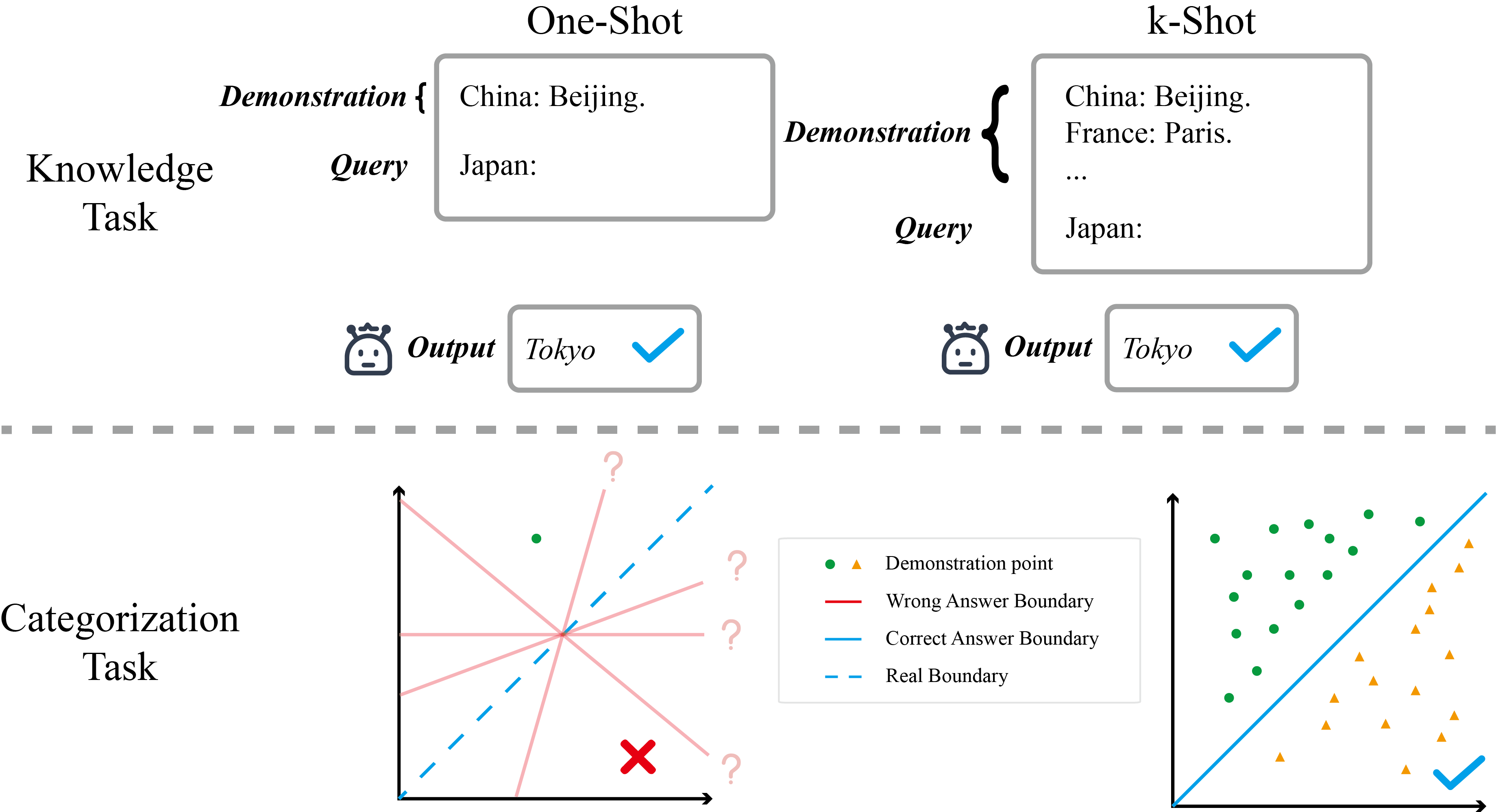
Figure 1: An illustration of the knowledge task and the categorization task. The knowledge task requires accessing LLM’s existing prior knowledge. In contrast, the categorization task needs given demonstrations. Therefore, the categorization task requires more demonstrations to accomplish the task.

2 Related Work

Neuroscience

Our work is inspired by studies from the field of neuroscience(Yamins, DiCarlo (2016); Richards et al. (2019); Barrett et al. (2019); Yousefi et al. (2023)) that explore the computational mechanisms underlying cognitive functions of the brain. The current study adopts a categorization task similar to what has been used widely in testing animals and humans in neuroscience. These experiments typically provide the demonstrations sequentially. Subjects learn the task through trial-and-error. This process is typically modeled as reinforcement learning (Niv (2009)). However, it has been shown that a system that stores behavior history could model the learning equally well without using explicit reinforcement learning (Zhang et al. (2018)). This is conceptually similar to ICL in LLMs. The demixed-PCA (dPCA) analysis used in our study is also initially developed for studying study how information is encoded in a high-dimensional space represented by population neuronal activities (Kobak et al. (2016)).

ICL

Brown et al. (2020) discovered that large-scale models like GPT-3 possess few-shot learning abilities, enabling them to perform reasoning across different tasks from just a few demonstrations. Meta-learning capabilities may be behind the models’ capability to efficiently adapt to new information (Dai et al. (2023)). It has been further proposed that transformers utilize gradient descent to perform linear regression tasks (Von Oswald et al. (2023); Akyürek et al. (2023); Ahn et al. (2024)). However, these studies involve learning specific linear regression tasks on toy models, and it is not clear if the conclusion may generalize. Another approach to understanding ICL in LLMs is to view pre-trained models as implicit Bayesian models, and the demonstrations provided in the prompts allow the model to compute the posteriors (Xie et al. (2022); Wang et al. (2023b); Ahuja et al. (2023)).

Task Vector

It is proposed that LLMs might be either compressing abstract rule information from demonstrations (Hendel et al. (2023)) or aggregating demonstration information layer-by-layer (Wang et al. (2023a)). These studies focused on tasks that can be solved in principle with one demonstration. An example is to tell the capital of a country. We term these tasks "knowledge tasks". Hendel et al. (2023) argued that ICL is achieved through a single task vector in the middle layers extracted from the demonstrations. In contrast, our research focuses on categorization tasks, which rely on multiple demonstrations. We leverage this distinction to emphasize a more general mechanism than "task vector" in ICL.

3 Task and Model

We mainly use a two-alternative categorization task to demonstrate the distributed rule vectors. In this task, the model is given a string of random characters, with the length varying between 1 and 10. The model should answer 0 when the string is shorter than 6 characters and 1 otherwise, e.g., "wkc->0, fezffgghijk->1, niaps->". The number of demonstrations ranges from 1 to 16. Several additional categorization tasks are also tested for comparisons (Table 1).

The knowledge task we use in the current study is the same task as in Hendel et al. (2023) and Wang et al. (2023a). The model should give the capital of a given country, e.g., the prompt "China->Beijing, Japan->Tokyo, German->" should lead to the answer "Berlin".

The model that we use in the experiments is LLaMA-7B (Touvron et al. (2023)).

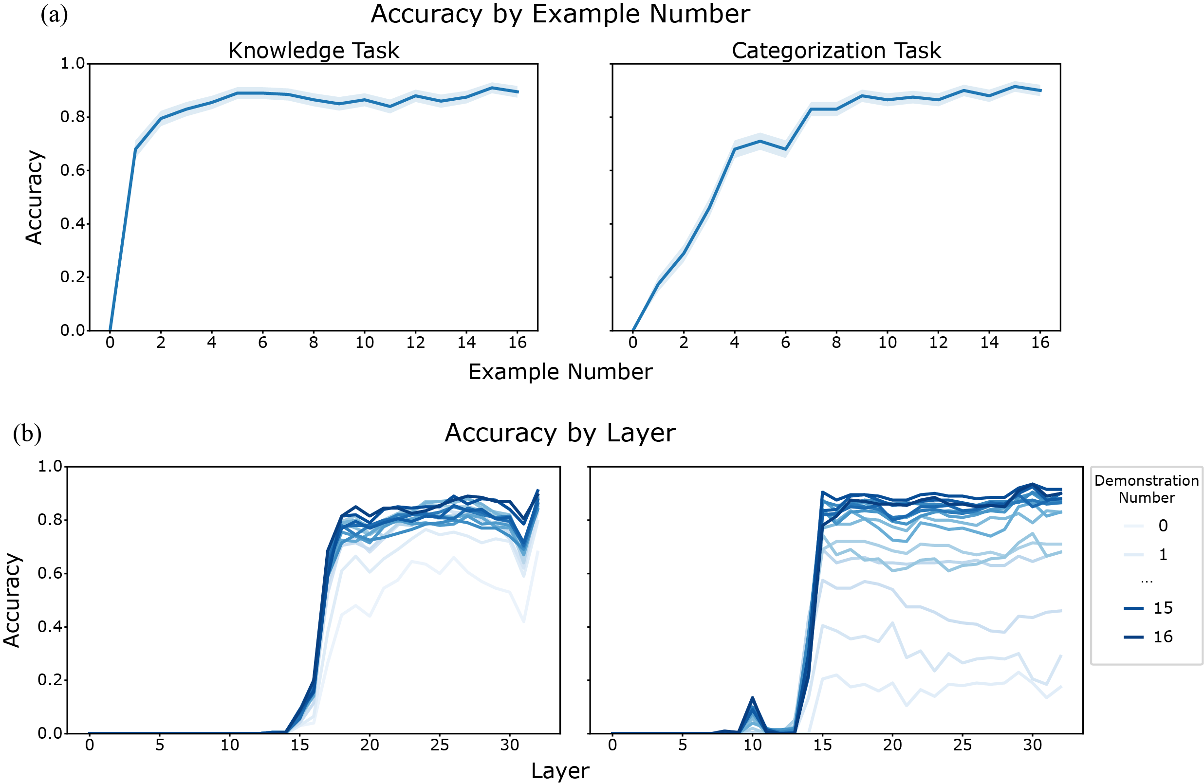
Figure 2: Model performance. (a) Model accuracy improves with more demonstrations. Left: knowledge task; Right: categorization task. (b) Accuracy increases sharply in the middle layers. The shades of blue indicate demonstration numbers. Left: knowledge task; Right: categorization task.

4 Results

4.1 Performance

As expected, the model can solve both tasks with a sufficient number of demonstrations (Figure 2). In the knowledge task, a single demonstration increases the accuracy from 0 to 70%, with further demonstrations providing only minor improvements. In contrast, the performance increase in the categorization task is much more gradual, reaching over 80% accuracy only when more than seven demonstrations are provided. This learning pattern is similar to how humans and animals acquire knowledge based on trial-and-error in these types of tasks (Zhang et al. (2018)).

We also investigate how the answer evolves and propagates through the model’s hidden layers. Using the same readout header, we extract the answer from each layer’s output (Hendel et al. (2023)) and plot the accuracy as a function of layer number (Figure 2). For both tasks, the accuracy exhibits a sudden jump in the middle layers. This trend is consistent across conditions with varying numbers of demonstrations, suggesting that the aggregation of information from multiple demonstrations does not require the processing in additional layers.

4.2 Saliency Score

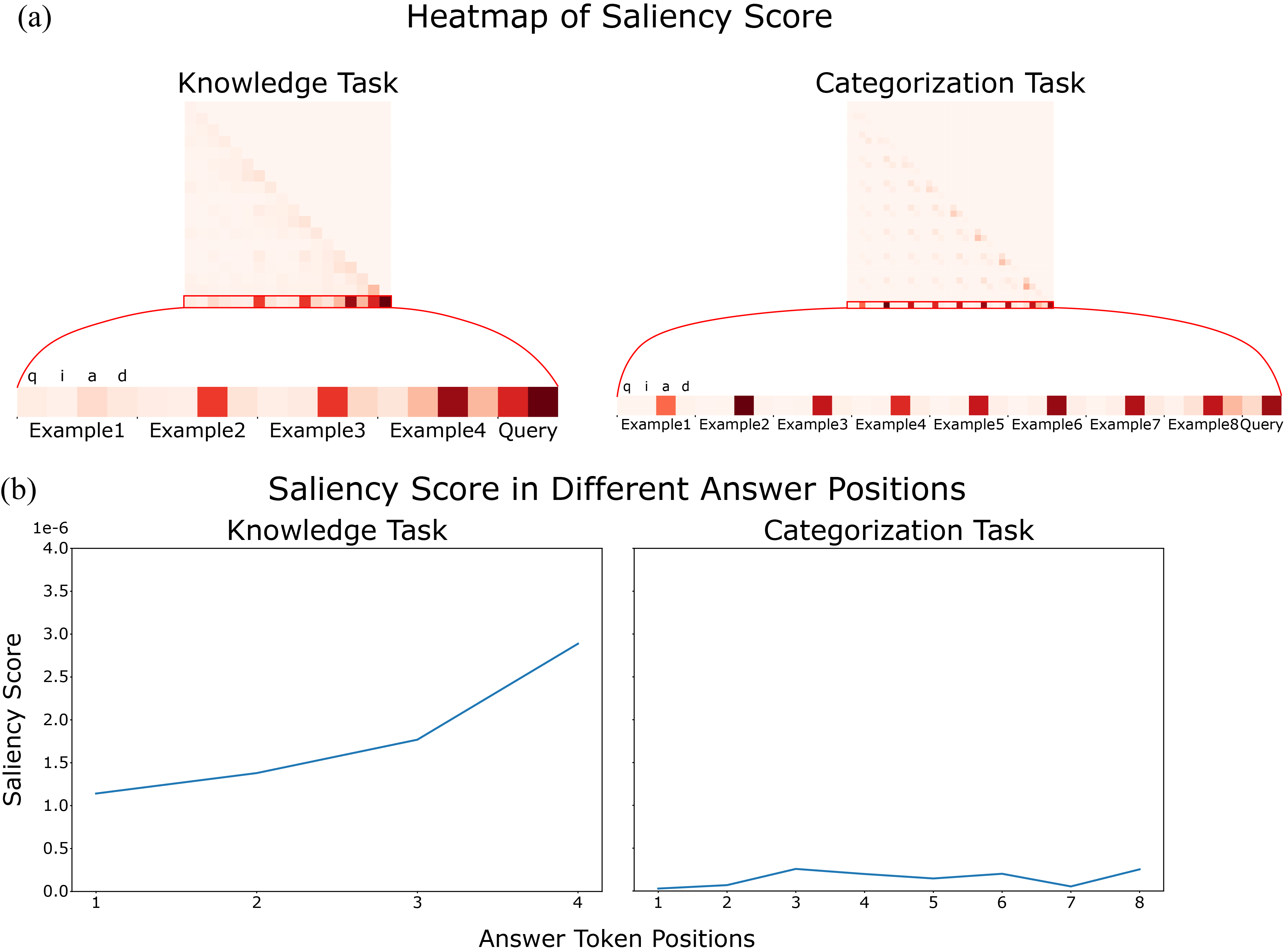
Figure 3: Saliency Score in the middle layers. (a) Saliency score shown as heatmaps. The color at each location shows the saliency score between the positions in the respective row and column. The last row, where the highest scores are observed, is amplified below, and q, i, a, d represents query, is, answer, and dot (separator between the demonstrations) positions. (b) The saliency score of the answer position of each demonstration. Left: knowledge task; Right: categorization task.

Next, we explore how information from the demonstrations is integrated to form an answer. In particular, we hypothesize that the attention pattern in the middle layers where there is a sharp increase in accuracy should be where the information integration occurs. We use the saliency score (Simonyan et al. (2013); Michel et al. (2019); Wang et al. (2023a)), defined as

$${I_{l}}=\left|{\sum\limits_{h}{{A_{h,l}}}\odot\frac{{\partial{\cal L}(x)}}{{\partial{A_{h,l}}}}}\right|,$$ (1)

to measure the contribution of attention between two tokens toward the output. Using layer 14 as a representative layer, we find that the saliency scores in both tasks are the highest between the answer position of the demonstrations and the is position of the final query, suggesting the information from the demonstrations converges to the token at the is position of the query (Figure 3a). Interestingly, the saliency score increases in the order of the demonstrations given in the knowledge task, suggesting that later demonstrations may provide more information and play a more important role. Such a trend is not found in the categorization task (Figure 3b).

The subtle difference between the tasks may have important implications. In the categorization task, all demonstrations are equally important for establishing the rule, while the knowledge task may depend mainly on a particular demonstration to deduce the rule (Figure 1).

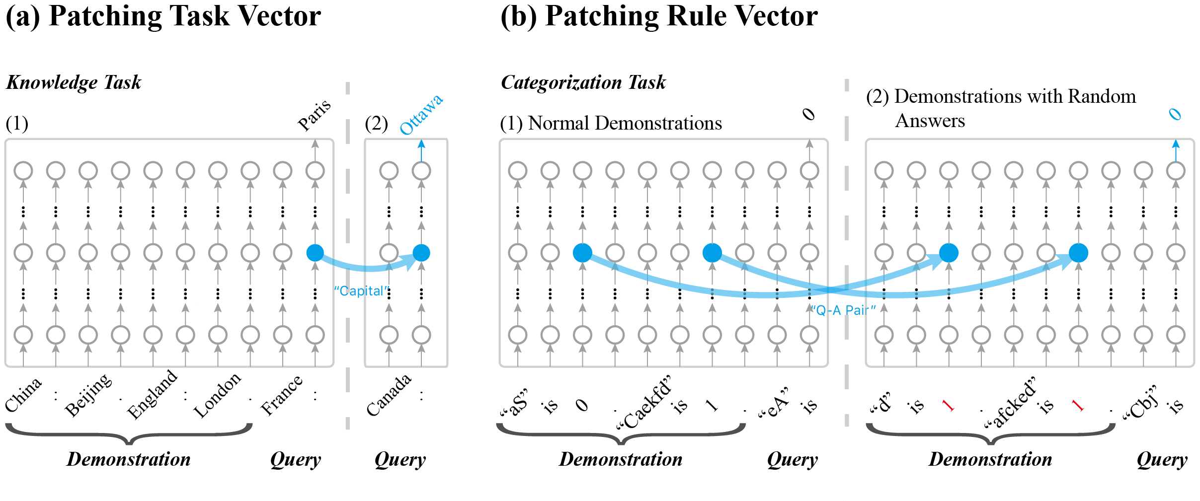
Figure 4: Patching experiments. (a) Patching the task vector. The token at the is position of the final query, the task vector, in a network receiving normal demonstrations is copied to a network performing 0-shot inference. (b) Patching the distributed rule vectors. The token at the answer position of each demonstration (rule vector) in a network receiving normal demonstrations is copied to a network receiving the same number of demonstrations but with random answers.

4.3 Task Vector

Previously, it was suggested that ICL creates a task vector, and patching the last position in the query with the task vector was sufficient for a model to perform zero-shot tasks (Hendel et al. (2023)). Here, we first investigate whether such a task vector exists in tasks with a distributed nature.

First, we confirm the finding of the task vector in the knowledge task. More specifically, given the input sequences $S=[Q_{0}I_{0}A_{0}D_{0},Q_{1}I_{1}A_{1}D_{1},...,Q_{J+1}I_{J+1}]$, where $Q_{j}$, $I_{j}$, $A_{j}$, and $D_{j}$ are the tokens for the query, the is, the answer and the dot of demonstration ${j\;(j=1,...,J)}$. The final query is denoted by ${Q_{J+1}}$, and is ${I_{J+1}}$. The task vector we use is in $I_{J+1}$. Note that this is different from the definition in Hendel et al. (2023), where the task vector is defined as the averaged $I_{J+1}$ token across all samples in the test set:

$$\theta_{task}=\frac{1}{N}\sum_{n=0}^{N}{I^{n}_{J+1}}$$ (2)

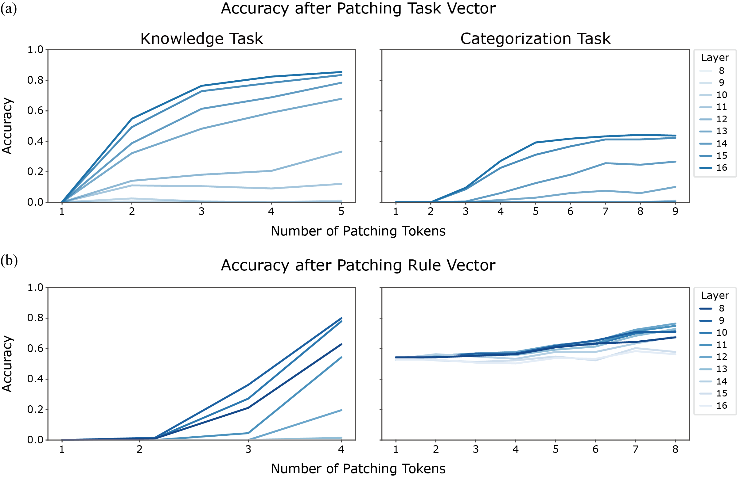
Figure 8: Patching effects are stronger with more demonstrations. (a) Patching with task vectors created with a larger number of demonstrations leads to better 0-shot performance. Blue shades indicate layer number. (b) Patching different numbers of rule vectors in 8-16 layers for the knowledge and the categorization task. Left: knowledge task; Right: categorization task.

We patch the network receiving dummy demonstrations with the task vector (Figure 4a). The patch, when applied in the appropriate layers, allows the network to perform 0-shot learning in the knowledge task (Figure 5a, left). Task vectors created with more demonstrations lead to higher accuracy (Supp Figure 8a). With task vectors based on three or more demonstrations, the 0-shot performance of the patched network is on par with that receiving the real demonstrations. The layers where the patch works the best coincide with the layers where we see the biggest jump in accuracy.

The same method, however, does not work well for the categorization task. The patch only allows the model to perform near the chance level, which is 50% (Figure 5a, right), suggesting that there is not such a task vector in the categorization task.

4.4 Distributed Rule Vectors

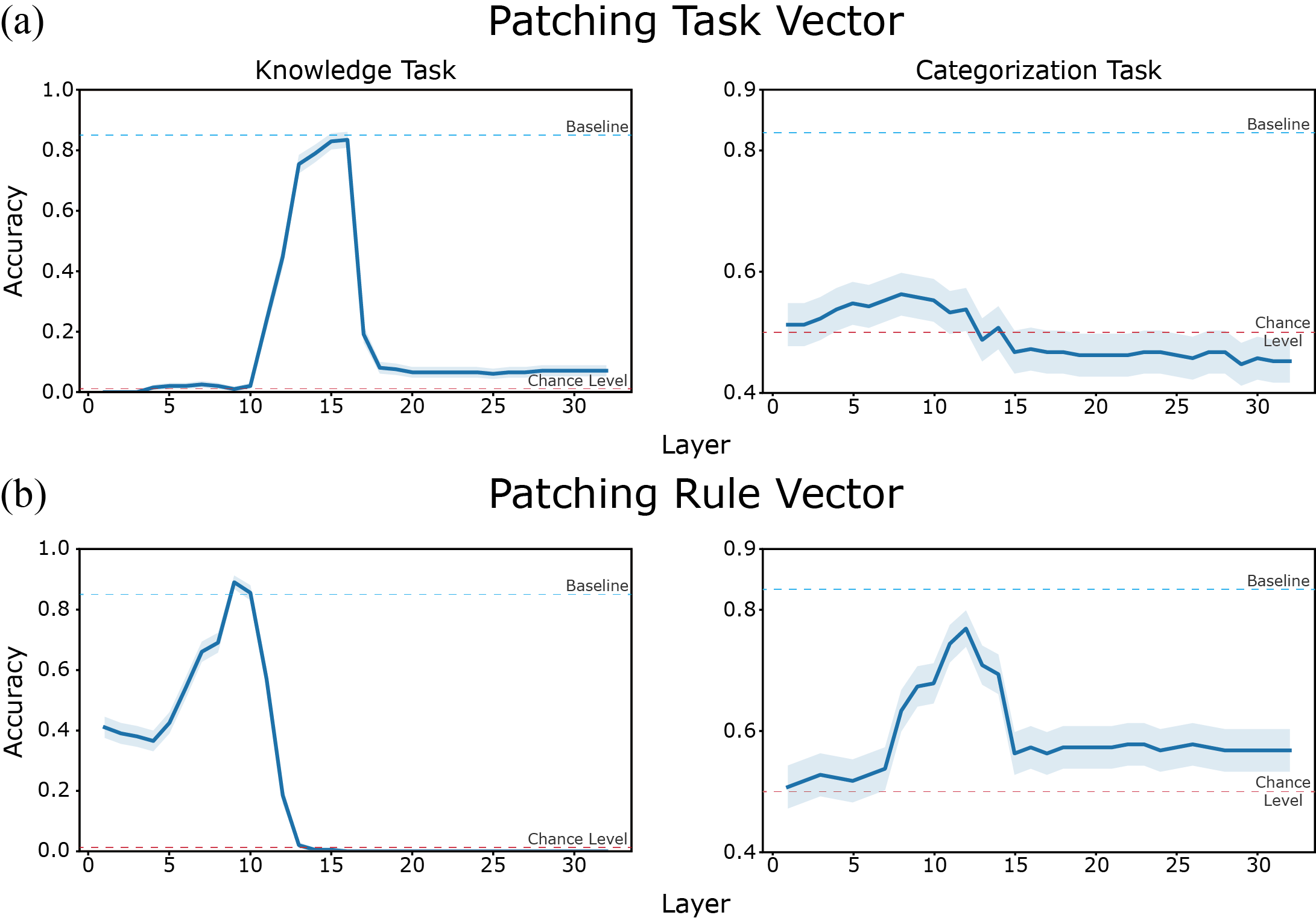
Figure 5: Patching the task vector and the rule vectors. (a) The accuracy of the network patched with the task vector in different layers in the knowledge and the categorization task. (b) The accuracy of the network patched with the distributed rule vectors in different layers in the knowledge and the categorization task. Left: knowledge task with 4 demonstrations. Right: categorization task with 8 demonstrations. Shading around the performance curve indicates standard error. Blue dash lines indicate the baseline performance, which is the network receiving normal demonstrations. Red dash lines indicate the chance level for the categorization task.

The failure of finding a task vector in the categorization task is consistent with the distributed nature of the task. Based on the saliency score analysis, we hypothesized that the task information is distributed across the demonstrations at their answer positions, which have the highest saliency scores. To test this idea, we patched the tokens at the answer positions in each layer of a network receiving dummy demonstrations. More specifically, given a dummy sequence $D=[Q_{0}^{d}I_{0}^{d}A_{0}^{d}D_{0}^{d},Q_{1}^{d}I_{1}^{d}A_{1}^{d}D_{1}^{d},...,Q_{J+1}^{d}I_{J+1}^{d}]$ and an original sequence $S=[Q_{0}I_{0}A_{0}D_{0},Q_{1}I_{1}A_{1}D_{1},...,Q_{J+1}I_{J+1}]$, we patch $A_{j}$ to $A_{j}^{d}$ as illustrated in Figure 4b, where $Q_{j}^{d}$ is a different query from $Q_{j}$, and $A_{j}^{d}$ is a random answer that provides no information for the task.

Categorization Rule	Demonstration	Baseline	Task Vector	Task Vector	Distributed
	Examples		(Average)	(Non Average)	Rule Vectors
String Length (Simple) 1 if len>5 else 0	abaabb->1, aab->0	0.78	0.61	0.57	0.66
String Length (Complex) 1 if len>5 else 0	aFeXGb->1, axvb->0	0.72	0.56	0.54	0.63
Digit 1 if digit>=5,else 0	4->0, 7->1	0.64	0.62	0.55	0.60
2-D data (8 demonstrations) 1 if y>=x,else 0	(0,1)->1, (7,4)->0	0.57	0.51	0.50	0.53
2-D data (16 demonstrations)	(0,1)->1, (7,4)->0	0.71	0.56	0.55	0.61

Table 1: Task Vector and Rule Vectors in a series of categorization task. Shown is the performance of the network receiving dummy demonstrations and patched with the average task vector of several samples, the task vector from a network receiving matching normal demonstrations, and the distributed rule vectors from a network receiving matching normal demonstrations. Baseline is the network receiving normal demonstrations. Simple strings only contain letters a and b, and complex strings contain all letters in both the capital and lower cases.

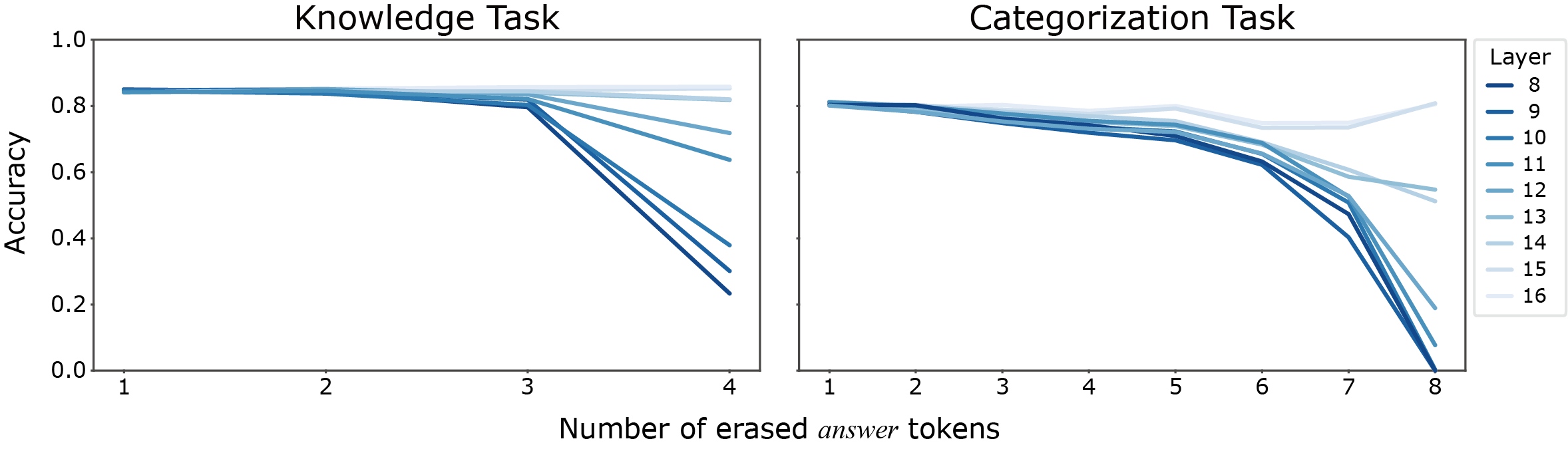
Figure 9: Model accuracy of ablated models.

Consistent with our hypothesis, patching these tokens in the middle layers rescues the performance of the model in the categorization task (Figure 5b, right). The more demonstrations are patched, the better the performance (Supp Figure 8b, right). The patched model reaches a performance comparable to the normal model. Directly resetting the tokens at the answer position in a normal network decreases the model’s performance gradually, confirming the distributed nature of the categorization task (Supp Figure 9). Note that the answers alone are insufficient for the model to extract the rule. The tokens at the answer positions also contain the information of the queries. Collectively, we term them the distributed rule vectors.

Interestingly, patching the answer positions also improves the network’s performance in the knowledge task, suggesting the distributed rule vectors also exist in this task. However, patching the task vector and patching the distributed rule vectors have the largest effects at different layers. (Figure 5ab, left). The shape of the accuracy curve suggests that the distributed rule vectors appear earlier in the network and then converge to a single task vector in later layers in the knowledge task. Such transition of information is not observed in the categorization task (Figure 5ab, right).

We carry out further experiments with different tasks. All of them require multiple demonstrations to establish the correct rule. The results are summarized in Table 1. Patching the distributed rule vectors all leads to better performance than patching the task vector in these tasks, even when we use the task vector computed from averaging across the entire dataset.

4.5 Abstract Rule Encoding

The patching experiments suggest that the information encoded in the rule vectors is crucial. But what exactly is encoded? Is it just the information regarding the question and the answer?

4.5.1 PCA

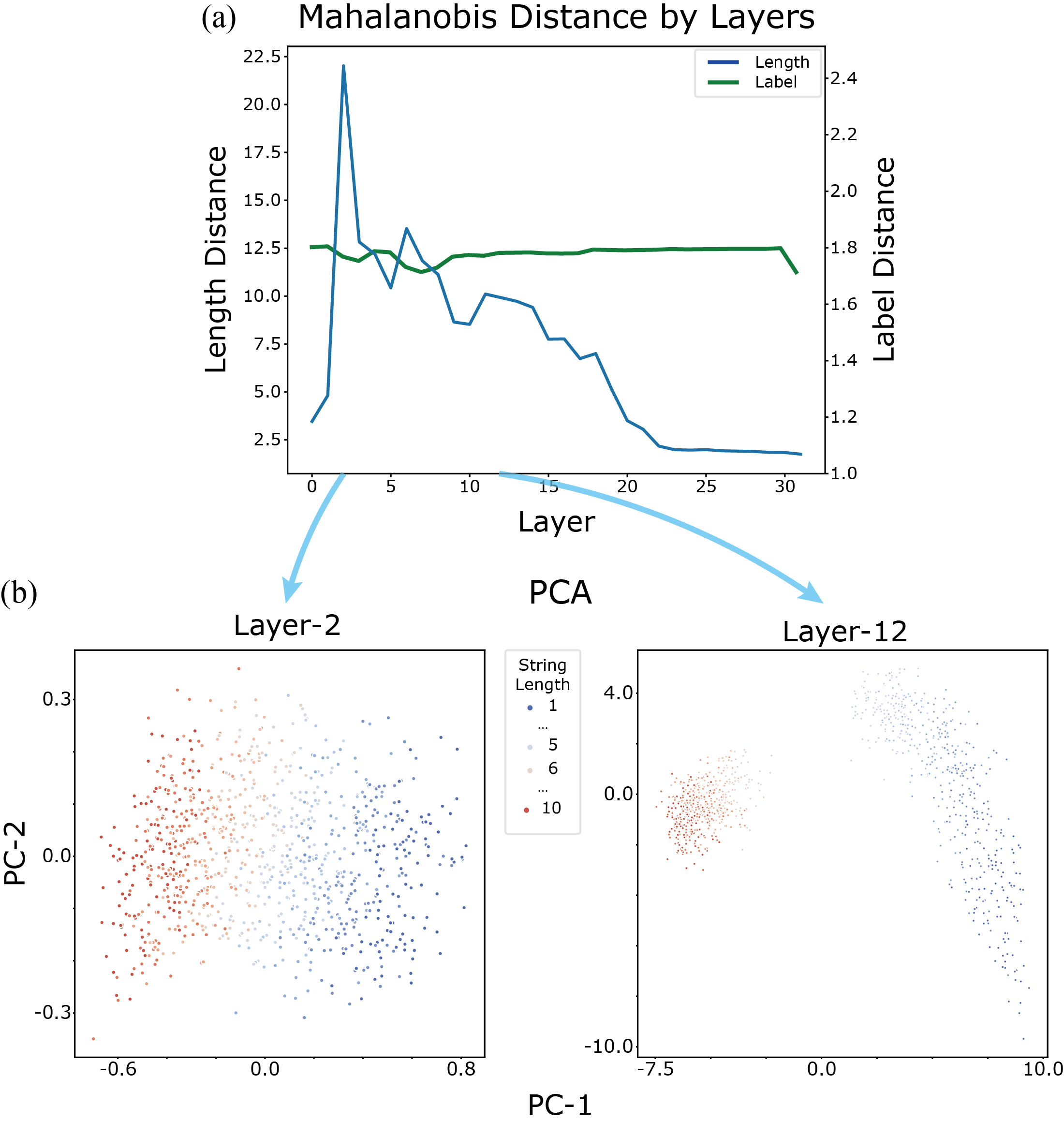
Figure 6: The encoding of string length and answer in rule vectors. (a) Plotted is the Mahalanobis distance of the clusters defined by the query string’s length (blue) and by the answer (green) in the space defined by the two largest PCA components of the rule vectors. Peaking at layer 2, the Mahalanobis distance for the string length gradually decreases across layers, indicating poorer segregation of the clusters and weaker encoding of string length in the rule vectors. (b) Two example rule vector spaces defined by the two largest PCA components. Blue and red indicate answers 0 and 1, and the contrast indicates string length. Notice that the segregation between the blue and red color is maintained across the layers, while the dots with different contrast (string length) are more mixed in the later layers (e.g. layer 12) than in the earlier layers (e.g. layer 2).

To further investigate the information encoded within the rule vectors, we first use principle component analysis (PCA) to examine the rule vectors in lower dimensions (Figure 6). We calculate the Mahalanobis distances between the clusters defined with string length and with answer for each layer’s rule vectors (Figure 6). The results suggest that the clusters of different string lengths are best segregated in the early layers, with the distance peaking at layer 2 and decreasing gradually. In comparison, the answer is encoded in the PCA space stably across layers. These trends differ from what is observed when we examine the effectiveness of patching applied to different layers. (Figure 5).

4.5.2 dPCA

To dig deep into the mismatch between the query and answer information encoding and the patching effectiveness, we carry out an experiment in which we selectively remove the string length information from the rule vectors. To do so, we first find the subspace that contains the string length information with dPCA, and then project the rule vectors onto the null space of the found subspace. This procedure erases all information from the subspace that contains the string length information while keeping the rest of information intact.

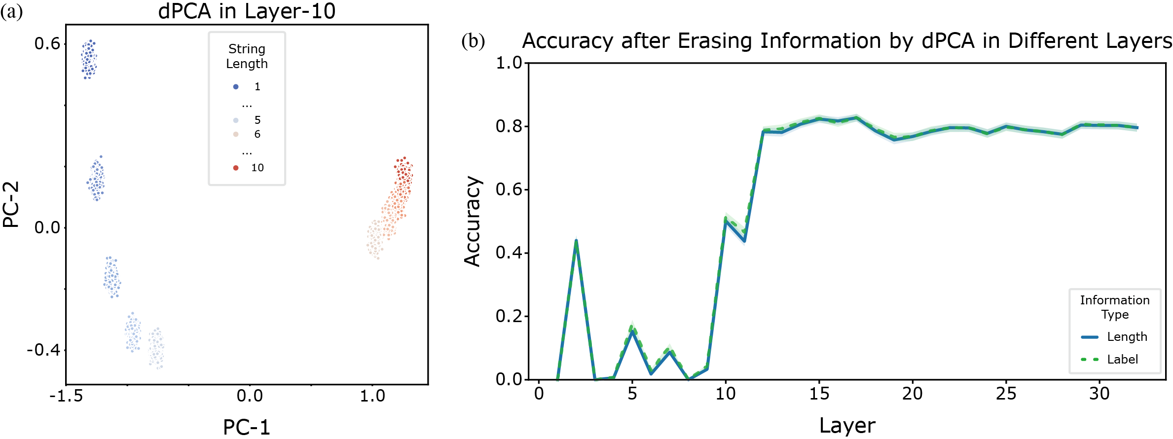
Figure 7: Selective removal of demonstration information with dPCA. (a) Using layer 10 as the example, both string length and answer information can be well captured in the 2-d dPCA space. (b) The model’s accuracy after string length information in rule vectors are removed in the dPCA space. Note the ablation is only effective in early layers, where the patching effects are small.

The results are shown in Figure 7. The selective information removal leads to poor performance when applied in the early layers. However, in the middle layers (e.g. layer 13), where the distributed rule vectors are found with the patching experiments, the same procedure leads to only minimal decrease in the network performance. These results suggest that within the rule vectors, the rule information is a high-level abstraction of the query-answer information that is not affected by the selective information removal.

5 Limitations

The current study is limited by the number of tasks that we tested. We also only perform the experiments in LLaMA. Other LLMs may yield different results.

6 Conclusion

Our study has expanded our understanding of ICL in LLMs. Unlike previous hypotheses suggesting the creation of a specific "task vector," our results demonstrate that LLMs employ a more general mechanism involving distributed rule vectors that encapsulate the relational information between queries and answers across multiple demonstrations. This indicates a more nuanced, distributed information processing to utilize multiple demonstrations to refine the extraction of rules in ICL.

7 Analysis Details

7.1 Framework and Dataset

We employ the LLaMA-7B from HuggingFace Touvron et al. (2023) as our primary model, and the model weights are also sourced from HuggingFace. No further processing on the weights is performed.

The task dataset can be found in supplemental material.

7.2 Mahalanobis Distance

Given a point $\mathbf{x}$ and a distribution with mean $\mathbf{\mu}$ and covariance matrix $\mathbf{\Sigma}$, the Mahalanobis distance $D_{M}$ from $\mathbf{x}$ to the distribution is defined as:

$$D_{M}(\mathbf{x})=\sqrt{(\mathbf{x}-\mathbf{\mu})^{T}\mathbf{\Sigma}^{-1}(\mathbf{x}-\mathbf{\mu})}$$

To calculate Mahalanobis distance, we first group the hidden states into different clusters based on the interested parameter, e.g. string length in our main task. Then we calculate the covariance in each cluster and compute the pairwise distance between each point outsideand inside the cluster.

7.3 dPCA

Following Kobak et al. (2016), we find a compressing matrix D and a decompressing matrix F by minimizing:

$$L_{dPCA}=||{\bf X_{L}}-{\bf FDX}||^{2}$$ (3)

where ${\bf X}$ is the $n\times{4096}$ activity matrix, ${\bf X_{L}}$ is a label average matrix. ${\bf X_{L}}$ has the same size as ${\bf X}$, but all the rows are replaced by the mean activity vector with the same label.

We then project the rule vectors onto the null space of the informative subspace:

$${\bf B}=Null({\bf D})$$ (4)

$$\tilde{{\bf X}}={\bf B}({\bf B}^{T}{\bf B})^{-1}{\bf B}^{T}{\bf X}$$ (5)

where ${\bf D}\in\mathbb{R}^{d\times{4096}}$ is the compression matrix, $Null(...)$ is the null space computation so that ${\bf D}Null({\bf D})=0$. $\tilde{\bf X}$ is the manipulated activity matrix. The mean is subtracted before the operation and then added back when we put the matrix back into the model.

7.4 Tokenization

Our experiments require us to retrieve tokens at specific positions. However, the tokenizer used with LLaMA generates variable numbers of tokens even for strings of the same length. Therefore, we insert a special character, e.g. "$\sim$", into the original input text to force the tokenizer to generate the same number of tokens for strings of the same length. We remove the token of these special characters after the tokenization step.

7.5 Accuracy Per Layers

When calculating accuracy per layer, we apply the final layer norm and the language model head to the hidden states in these layers. This was introduced in Hendel et al. (2023).

7.6 Evaluation Details

We use 5000 samples for calculating network performance. PCA and dPCA analyses are done with 1000 samples. More samples produce similar results.

All experiments are done with a single V100 GPU. Accuracy is evaluated with the token with the largest logit without temperature or any other probabilistic sampling methods.

Appendix A Appendix: Supplemental Material

A.1 Patching Accuracy vs. Number of Demonstrations

A.2 Ablation at Answer Position

Here we perform an ablation experiment by setting the token at the answer positions of the demonstrations to 0. For the knowledge task, we have to destroy the answer position of all demonstrations to see the effects. For the categorization task, the performance drop is much more gradual as we increase the number of ablated answer tokens, suggesting a distributed mechanism.

References

- Ahn et al. (2024) Ahn Kwangjun, Cheng Xiang, Daneshmand Hadi, Sra Suvrit. Transformers learn to implement preconditioned gradient descent for in-context learning // Advances in Neural Information Processing Systems. 2024. 36.
- Ahuja et al. (2023) Ahuja Kabir, Panwar Madhur, Goyal Navin. In-context learning through the bayesian prism // arXiv preprint arXiv:2306.04891. 2023.
- Akyürek et al. (2023) Akyürek Ekin, Schuurmans Dale, Andreas Jacob, Ma Tengyu, Zhou Denny. What Learning Algorithm Is In-Context Learning? Investigations with Linear Models. V 2023.
- Barrett et al. (2019) Barrett David GT, Morcos Ari S, Macke Jakob H. Analyzing biological and artificial neural networks: challenges with opportunities for synergy? // Current opinion in neurobiology. 2019. 55. 55–64.
- Binz, Schulz (2023) Binz Marcel, Schulz Eric. Using cognitive psychology to understand GPT-3 // Proceedings of the National Academy of Sciences. 2023. 120, 6. e2218523120.
- Brown et al. (2020) Brown Tom B, Mann Benjamin, Ryder Nick, Subbiah Melanie, Kaplan Jared. Language Models Are Few-Shot Learners // NeurIPS. 2020.
- Dai et al. (2023) Dai Damai, Sun Yutao, Dong Li, Hao Yaru, Ma Shuming. Why Can GPT Learn In-Context? Language Models Implicitly Perform Gradient Descent as Meta-Optimizers. V 2023.
- Dong et al. (2023) Dong Qingxiu, Li Lei, Dai Damai, Zheng Ce, Wu Zhiyong. A Survey on In-Context Learning. VI 2023.
- Hendel et al. (2023) Hendel Roee, Geva Mor, Globerson Amir. In-Context Learning Creates Task Vectors. X 2023.
- Ilharco et al. (2022) Ilharco Gabriel, Ribeiro Marco Tulio, Wortsman Mitchell, Gururangan Suchin, Schmidt Ludwig, Hajishirzi Hannaneh, Farhadi Ali. Editing models with task arithmetic // arXiv preprint arXiv:2212.04089. 2022.
- Kobak et al. (2016) Kobak Dmitry, Brendel Wieland, Constantinidis Christos, Feierstein Claudia E, Kepecs Adam, Mainen Zachary F, Qi Xue-Lian, Romo Ranulfo, Uchida Naoshige, Machens Christian K. Demixed principal component analysis of neural population data // elife. 2016. 5. e10989.
- Lester et al. (2021) Lester Brian, Al-Rfou Rami, Constant Noah. The power of scale for parameter-efficient prompt tuning // arXiv preprint arXiv:2104.08691. 2021.
- Liu et al. (2023) Liu Pengfei, Yuan Weizhe, Fu Jinlan, Jiang Zhengbao, Hayashi Hiroaki, Neubig Graham. Pre-train, prompt, and predict: A systematic survey of prompting methods in natural language processing // ACM Computing Surveys. 2023. 55, 9. 1–35.
- Michel et al. (2019) Michel Paul, Levy Omer, Neubig Graham. Are sixteen heads really better than one? // Advances in neural information processing systems. 2019. 32.
- Niv (2009) Niv Yael. Reinforcement learning in the brain // Journal of Mathematical Psychology. 2009. 53, 3. 139–154.
- Richards et al. (2019) Richards Blake A, Lillicrap Timothy P, Beaudoin Philippe, Bengio Yoshua, Bogacz Rafal, Christensen Amelia, Clopath Claudia, Costa Rui Ponte, Berker Archy de, Ganguli Surya, others . A deep learning framework for neuroscience // Nature neuroscience. 2019. 22, 11. 1761–1770.
- Simonyan et al. (2013) Simonyan Karen, Vedaldi Andrea, Zisserman Andrew. Deep inside convolutional networks: Visualising image classification models and saliency maps // arXiv preprint arXiv:1312.6034. 2013.
- Touvron et al. (2023) Touvron Hugo, Lavril Thibaut, Izacard Gautier, Martinet Xavier, Lachaux Marie-Anne, Lacroix Timothée, Rozière Baptiste, Goyal Naman, Hambro Eric, Azhar Faisal, others . Llama: Open and efficient foundation language models // arXiv preprint arXiv:2302.13971. 2023.
- Von Oswald et al. (2023) Von Oswald Johannes, Niklasson Eyvind, Randazzo Ettore, Sacramento João, Mordvintsev Alexander, Zhmoginov Andrey, Vladymyrov Max. Transformers learn in-context by gradient descent // International Conference on Machine Learning. 2023. 35151–35174.
- Wang et al. (2023a) Wang Lean, Li Lei, Dai Damai, Chen Deli, Zhou Hao. Label Words Are Anchors: An Information Flow Perspective for Understanding In-Context Learning. XII 2023a.
- Wang et al. (2023b) Wang Xinyi, Zhu Wanrong, Saxon Michael, Steyvers Mark, Wang William Yang. Large language models are implicitly topic models: Explaining and finding good demonstrations for in-context learning // Workshop on Efficient Systems for Foundation Models@ ICML2023. 2023b.
- Wei et al. (2022) Wei Jason, Wang Xuezhi, Schuurmans Dale, Bosma Maarten, Xia Fei, Chi Ed, Le Quoc V, Zhou Denny, others . Chain-of-thought prompting elicits reasoning in large language models // Advances in neural information processing systems. 2022. 35. 24824–24837.
- Xie et al. (2022) Xie Sang Michael, Raghunathan Aditi, Liang Percy, Ma Tengyu. An Explanation of In-Context Learning as Implicit Bayesian Inference. VII 2022.
- Yamins, DiCarlo (2016) Yamins Daniel LK, DiCarlo James J. Using goal-driven deep learning models to understand sensory cortex // Nature neuroscience. 2016. 19, 3. 356–365.
- Yousefi et al. (2023) Yousefi Safoora, Betthauser Leo, Hasanbeig Hosein, Millière Raphaël, Momennejad Ida. Decoding In-Context Learning: Neuroscience-inspired Analysis of Representations in Large Language Models // arXiv preprint arXiv:2310.00313. 2023.
- Zhang et al. (2018) Zhang Zhewei, Cheng Zhenbo, Lin Zhongqiao, Nie Chechang, Yang Tianming. A neural network model for the orbitofrontal cortex and task space acquisition during reinforcement learning // PLOS Computational Biology. 2018. 14, 1. e1005925.