State-Compensation-Linearization-Based Stability Margin Analysis for a Class of Nonlinear Systems: A Data-Driven Method

Abstract

The classical stability margin analysis based on the linearized model is widely used in practice even in nonlinear systems. Although linear analysis techniques are relatively standard and have simple implementation structures, they are prone to misbehavior and failure when the system is performing an off-nominal operation. To avoid the drawbacks and exploit the advantages of linear analysis methods and frequency-domain stability margin analysis while tackling system nonlinearity, a state-compensation-linearization-based stability margin analysis method is studied in the paper. Based on the state-compensation-linearization-based stabilizing control, the definition and measurement of the stability margin are given. The $\mathcal{L_{\text{$2$}}}$ gain margin and $\mathcal{L_{\text{$2$}}}$ time-delay margin for the closed-loop nonlinear system with state-compensation-linearization-based stabilizing control are defined and derived approximatively by the small-gain theorem in theory. The stability margin measurement can be carried out by the frequency-sweep method in practice. The proposed method is a data-driven method for obtaining the stability margin of nonlinear systems, which is practical and can be applied to practical systems directly. Finally, three numerical examples are given to illustrate the effectiveness of the proposed method.

I Introduction

With the development of society, more and more fields demand high safety and reliability. However, uncertainties are ubiquitous and inevitable for almost all practical systems [1]. In practice, it is not enough to just know whether a system is stable or not. It needs to be further analyzed how stable and robust a system is. As a quantitative indicator of the systems’ relative stability and robustness, stability margin (SM) [2, 3] is widely used in control engineering. Uncertainties, such as delay or unmodeled higher-order dynamics, can be intuitively captured by SM, which can be further adopted as a safety metric for danger monitoring, controller tuning [4, 5], filter and compensator design [6], etc. Thus, SM is important in the analysis and design of control systems.

There has been much research on SM. For single-input single-output (SISO) linear time-invariant (LTI) systems, the classic SM, namely the gain margin (GM) and phase margin (PM), is well defined and understood [7]. It is a class of classic frequency-domain SM, which is straightforward, intuitive, and has clear physical meaning. Thus, the classic SM is popular and widely adopted by control engineers. Reference [1] discussed robust SM in the field of robust control. $\mu$-analysis is popular among multivariable systems, in which the singular-value-based stability margin is defined as a robust SM [8]. In order to deal with the modeling uncertainties described by coprime factor perturbations, the gap metric [9] and its variant, the $\nu$-gap [10], provide quantitative measures of robustness stability. Time-delay SMs for the control of processes with uncertain delays were investigated in [11]. However, these robust SMs are mostly applicable to linear systems.

For nonlinear systems, SM analysis becomes more complex and difficult. The classic frequency-domain SM is inapplicable because frequency-domain analysis and synthesis cannot be directly carried out in the presence of nonlinearity. The circle criterion, Popov’s criterion, and Kalman-Yakubovich-Popov (KYP) lemma are used for the absolute stability analysis of a nonlinear system in the frequency domain when it is a feedback connection of a linear dynamical system and a nonlinear element satisfying the sector condition [12, 13, 14], in which Lyapunov functional approach is often used and further formulated in the form of linear matrix inequalities (LMIs). However, few SMs have been defined therein. Based on singular perturbation analysis, the singular perturbation margin and generalized gain margin were proposed in [15]. These metrics are bijective counterparts of GM and PM. Besides, gain, sector, and disk margins [16, 17] are studied in terms of different stability specifications, such as Lyapunov stability, $\mathcal{H}_{\infty}$ stability, or input-to-state stability. Although many SM definitions have been proposed for nonlinear systems, most SMs for nonlinear systems require time-domain definitions or calculations, which are complex and not easy to apply in practice.

In practice, it is a common and mature practice to utilize linear control techniques at discrete operating points within the operating envelope or along a nominal trajectory, and then classic frequency-domain SM is used to certify the designed controllers at the discrete points[3, 18]. The drawback of this approach is that the obtained SM may be unreliable when the assumption of benign nonlinearity fails in operation. Another common choice is experimental methods, for example, Monte Carlo simulations. However, most experimental methods are time-consuming and costly. What is worse, the worst situation may not occur, which leads to an inaccurate estimate of SM.

On the whole, while SM is of importance in control design practice, it is hard to find the SM of a large number of nonlinear systems, which motivates us to carry out this research. In this paper, a state-compensation-linearization-based stabilizing control from [19] is utilized for a class of nonlinear systems. This stabilizing control can put all the uncertainties in the primary linear system and compensate for all the nonlinearity in the secondary nonlinear system, which can make the following SM analysis for nonlinear systems easier. After state-compensation-linearization-based stabilizing control, SM analysis and measurement are next focused. Thanks to the developed control framework, frequency-domain SM analysis methods are applicable to the resulting nonlinear systems. The SM analysis can be divided into two steps. First, the SM for the primary system (an MIMO linear system) is derived by using the small-gain theorem. We have proposed a simple and practical data-driven stability margin analysis method for linear multivariable systems in [20]. Second, the SM for the whole system (an MIMO nonlinear system) is derived based on the small-gain theorem. Both SMs can be obtained by frequency-sweep experimental methods, which are preferable to calculation methods in practice. Based on these, the final SM can be determined. In the end, the whole procedure of the SCLC and SM analysis is summarized.

The main contributions of this paper lie in: New SMs are defined based on SCLC, and the corresponding measurement can be implemented by real experiments (e.g., frequency-sweep experiments), not only numerical calculation. The SM measurement by frequency-sweep experiments is data-driven, which approaches reality more. Owing to SCLC, frequency-domain SM analysis is extended smoothly to nonlinear systems. Furthermore, a complete design and analysis procedure in terms of robustness and stability for a class of nonlinear systems is presented, which is practical and can be applied to practical systems directly.

The paper is organized as follows. Section II gives the problem formulation including the considered system model and the objectives. Then, how to design a state-compensation-linearization-based stabilizing controller is recalled briefly in Section III. Next, the state-compensation-linearization-based SM analysis and measurement are given in IV. In Section V, simulations are performed to demonstrate the effectiveness and practicability of the proposed method. In the end, Section VI presents the conclusions.

II Problem Formulation

Consider a class of MIMO nonlinear systems as

$$\dot{\mathbf{x}}(t)=\mathbf{A\mathbf{x}}(t)+\mathbf{f}(\mathbf{x}(t))+\mathbf{B}\mathbf{\boldsymbol{\mu}}(t),\mathbf{x}(0)=\mathbf{x}_{0}.$$ (1)

Here $\mathbf{A}\in\mathbb{R}^{n\times n}$ is a stable constant matrix, $\mathbf{B}\in\mathbb{R}^{n\times m}$ is a constant matrix, $\mathbf{f}(\cdot):\mathbb{R}^{n}\rightarrow\mathbb{R}^{n}$ is a nonlinear function vector with $\mathbf{f}(\mathbf{0})=\mathbf{0}$, $\mathbf{x}(t)\in\mathbb{R}^{n}$ is the state vector, and $\mathbf{\boldsymbol{\mu}}(t)\in\mathbb{R}^{m}$ is the actual control input.

We define the gain and time-delay margins by putting a complex diagonal multiplicative perturbation $\mathbf{I}_{{m}}+\Delta(s)$ at the plant input, namely

$$\mathbf{\boldsymbol{\mu}}(s)=(\mathbf{I}_{{m}}+\Delta(s))\mathbf{u}(s)$$ (2)

where $\mathbf{u}(t)\in\mathbb{R}^{m}$ is the designed control input, $\mathbf{I}_{{m}}\in\mathbb{R}^{m\times m}$ is an identity matrix, and $\Delta(s)\in\mathbb{R}^{m\times m}$ is the artificial unmodeled dynamics (it does not exist but is introduced only for the stability margin analysis, and can be regarded as a “stability margin gauge” [15]). For system (1), the following assumptions are made.

Assumption 1. The pair $(\mathbf{A},\mathbf{B})$ is controllable .

Assumption 2. The system state is measurable.

Remark 1. Noteworthy, there are no restrictions on the function $\mathbf{f}(\mathbf{x}(t))$. For general systems $\mathbf{x}(t)=\mathbf{F}(x)+\mathbf{B}\mathbf{\mu}(t)$ which do not satisfy the form (1), by letting $\mathbf{A}=\left.(\partial(\mathbf{F}(\mathbf{x}))/(\partial\mathbf{x}))\right|_{\mathbf{x}=\mathbf{0}}$, $\mathbf{f}(\mathbf{x})=\mathbf{F}(\mathbf{x})-\mathbf{A}\mathbf{x}$, they can be transformed into the considered systems in the form of (1). Therefore, the form (1) is more general.

Objective 1. Under Assumptions 1-2, the first objective is to propose a controller $\mathbf{u}(t)=\mathbf{C}(\mathbf{x}(t))$ to make $\mathbf{x}\in\mathcal{L_{\text{$2$}}^{\text{$n$}}}$ under any initial condition $\mathbf{x}_{0}$ when $\Delta(s)=\mathbf{0}$.

Before introducing the next objective, the following stability margin definition is introduced first.

Definition 1. Given any $\Delta(s)\equiv\text{diag}\left(\gamma_{1},\gamma_{2},\ldots,\gamma_{m}\right)$, $\left|\gamma_{i}\right|\leq\gamma_{\text{max}}$, $i=1,2,\ldots m$, if the state of the closed-loop system composed by (1), (2) and $\mathbf{u}(t)=\mathbf{C}(\mathbf{x}(t))$ satisfies $\mathbf{x}\in\mathcal{L_{\text{$2$}}^{\text{$n$}}}$ for any initial condition $\mathbf{x}_{0}$, then the closed-loop system with $\Delta(s)$ is said to have the $\mathcal{L_{\text{$2$}}}$ gain margin $\gamma_{\text{max}}$. Given any $\Delta(s)=\text{diag}\left(\text{e}^{-s\tau_{1}}-1,\text{e}^{-s\tau_{2}}-1,\ldots,\text{e}^{-s\tau_{m}}-1\right)$, $0\leq\tau_{i}\leq\tau_{\text{max}}$, $i=1,2\cdots m$, if the state of the closed-loop system composed by (1), (2) and $\mathbf{u}(t)=\mathbf{C}(\mathbf{x}(t))$ satisfies $\mathbf{x}\in\mathcal{L_{\text{$2$}}^{\text{$n$}}}$ for any initial condition $\mathbf{x}_{0}$, then the closed-loop system with $\Delta(s)$ is said to have the $\mathcal{L_{\text{$2$}}}$ time-delay margin $\tau_{\text{max}}$.

Objective 2 The other objective is to determine the $\mathcal{L_{\text{$2$}}}$ gain margin and $\mathcal{L_{\text{$2$}}}$ time-delay margin for the resulting closed-loop nonlinear system.

III State-Compensation-Linearization-Based Stabilizing Control

The state-compensation-linearization-based (or say additive-state-decomposition-based) stabilizing control framework proposed in [19] can be used to propose a controller $\mathbf{u}(t)=\mathbf{C}(\mathbf{x}(t))$ to make $\mathbf{x}\in\mathcal{L_{\text{$2$}}^{\text{$n$}}}$ under any initial condition $\mathbf{x}_{0}$ when $\Delta(s)=\mathbf{0}$. In the following, for convenience, we will omit the variables $t,s$ except when necessary.

III-A Additive State Decomposition

Consider system (1) as the original system. First, the primary system is chosen as follows:

$$\mathbf{\dot{x}}_{\text{p}}=\mathbf{A}\mathbf{x}_{\text{p}}+\mathbf{B}\mathbf{\boldsymbol{\mu}}_{\text{p}},\mathbf{x}_{\text{p}}(0)=\mathbf{x}_{0}$$ (3)

where

$$\mathbf{\boldsymbol{\mu}}_{\text{p}}=(\mathbf{I}_{{m}}+\Delta)(\mathbf{u}_{\text{p}}+\mathbf{u}_{\text{s}})-\mathbf{u}_{\text{s}}$$ (4)

and $\mathbf{u}_{\text{s}}\triangleq\mathbf{u}-\mathbf{u}_{\text{p}}\in\mathbb{R}^{{m}}$ is the control for the secondary system in the following. Then, the secondary system is determined by subtracting the primary system (3) from the original system (1), and it follows that

$$\mathbf{\dot{x}}_{\text{s}}=\mathbf{A\mathbf{x}}_{\text{s}}+\mathbf{f}(\mathbf{x}_{\text{p}}+\mathbf{x}_{\text{s}})+\mathbf{B}\mathbf{u}_{\text{s}},\mathbf{x}_{\text{s}}(0)=\mathbf{0}.$$ (5)

If $\mathbf{x}_{\text{p}}=\mathbf{0}$, then $(\mathbf{x}_{\text{s}},\mathbf{u}_{\text{s}})=\mathbf{0}$ is an equilibrium point of (5).

An observer is proposed to estimate $\mathbf{x}_{\text{p}}$ and $\mathbf{x}_{\text{s}}$ in (3), (5) as follows:

$$\dot{\mathbf{\mathbf{\hat{\mathbf{x}}}}}_{\text{s}} =\mathbf{A}\hat{\mathbf{x}}_{\text{s}}+\mathbf{f}(\mathbf{x})+\mathbf{B}\mathbf{\mathbf{u}_{\text{s}}},\hat{\mathbf{x}}_{\text{s}}(0)=\mathbf{0}$$ (6)

$$\hat{\mathbf{x}}_{\text{p}} =\mathbf{x}-\mathbf{\hat{x}}_{\text{s}}.$$ (7)

Then $\hat{\mathbf{x}}_{\text{p}}=\mathbf{x}_{\text{p}}$ and $\mathbf{\hat{x}}_{\text{s}}=\mathbf{x}_{\text{s}}$. The proof can refer to [19].

III-B Stabilizing Control

In the control design, we first ignore the unmodeled dynamics $\Delta$ in (1), namely $\Delta=\mathbf{0}$ (Objective 1). However, it will appear in the stability margin analysis (Objective 2). When $\Delta=\mathbf{0}$, in the primary system (3), we have

$$\mathbf{\boldsymbol{\mu}}_{\text{p}}=\mathbf{u}_{\text{p}}.$$

• Problem 1 Consider the primary system, and the dynamic of which is described by (3) with $\Delta=\mathbf{0}$. Design the primary controller as

  $$\mathbf{u}_{\text{p}}=\mathcal{L}^{-1}(\mathbf{H}(s)\mathbf{K}\mathbf{x_{\text{p}}}(s))$$ (8)

  such that $\mathbf{x_{\text{p}}}\in\mathcal{L_{\text{$2$}}^{\text{$n$}}}$, where H(s) is a stable transfer function matrix, $\mathcal{L}^{-1}$ denotes the inverse Laplace transformation, and state feedback matrix $\mathbf{K\in\mathbb{R}^{\text{$m\times n$}}}$.

• Problem 2 Consider the secondary system, and the dynamic of which is described by (5). Design the secondary controller as

  $$\mathbf{u}_{\text{s}}=\mathbf{L}(\mathbf{x_{\text{p}}},\mathbf{x_{\text{s}}})$$ (9)

  such that $\mathbf{x_{\text{s}}}\in\mathcal{L_{\text{$2$}}^{\text{$n$}}}$, where $\mathbf{L}(\cdot,\cdot)$ is a nonlinear function.

With the solutions to the two problems in hand, we can state

Theorem 1 For system (1) with $\Delta=\mathbf{0}$ under Assumptions 1-2, suppose (i) Problems 1-2 are solved; (ii) the controller for system (1) with $\Delta=\mathbf{0}$ is designed as

$$\mathbf{\dot{\mathbf{\mathbf{\hat{x}}}}}_{\text{s}} =\mathbf{A}\hat{\mathbf{x}}_{\text{s}}+\mathbf{f}(\mathbf{x})+\mathbf{B}\mathbf{\mathbf{u}_{\text{s}}},\hat{\mathbf{x}}_{\text{s}}(0)=\mathbf{0}$$

$$\hat{\mathbf{x}}_{\text{p}} =\mathbf{x}-\mathbf{\hat{x}}_{\text{s}}$$

$$\mathbf{\boldsymbol{\mu}} =\mathbf{C}\left(\mathbf{x}\right)=\mathcal{L}^{-1}(\mathbf{H}(s)\mathbf{K}\hat{\mathbf{x}}_{\text{p}}(s))+\mathbf{L}(\hat{\mathbf{x}}_{\text{p}},\mathbf{\hat{x}}_{\text{s}}).$$ (10)

Then, the state of system (1) with $\Delta=\mathbf{0}$ satisfies $\mathbf{x}\in\mathcal{L_{\text{$2$}}^{\text{$n$}}}$.

The controllers for the primary system and the secondary system are shown in Fig. 1(b) for analysis. As shown, when $\Delta=\mathbf{0}$, the primary system is independent of the secondary system. However, the secondary system depends on the state of the primary system. In practice, the two controllers are combined to control the original system as shown in Fig. 1(a).

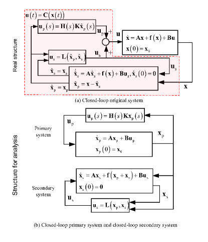
Figure 1: When unmodeled dynamics $\Delta=\mathbf{0}$, Fig. 1(a) shows the real closed-loop system corresponding to the original system, which can be decomposed into the two closed-loop subsystems in Fig. 1(b) for analysis.

So far, we have solved Objective 1 by Theorem 1 and derived the controller $\mathbf{C}\left(\mathbf{x}\right)$ as in (10). However, it is not sufficient just know whether a system is stable or unstable. If a system is just barely stable, then a small perturbation in a system parameter could push the system over the edge. Thus, one often wants to design systems with some robust stability margin. In the following, the $\mathcal{L_{\text{$2$}}}$ gain margin and $\mathcal{L_{\text{$2$}}}$ time-delay margin will be used to measure how stable a system is, and how to determine them is further concerned (Objective 2).

IV State-Compensation-Linearization-Based Stability Margin Analysis

IV-A Stability Margin Analysis

From the definition of $\mathbf{\boldsymbol{\mu}}_{\text{p}}$ in (4), we have

$$\mathbf{\boldsymbol{\mu}}_{\text{p}}=(\mathbf{I}_{{m}}+\Delta)\mathbf{u}_{\text{p}}+\Delta\mathbf{u}_{\text{s}}.$$

In the presence of $\Delta$, Fig. 1 is modified to Fig. 2. Because of $\Delta$, the primary system and the secondary system are interconnected, namely the primary system is dependent on the secondary system and the secondary system is, in turn, dependent on the primary system as shown in Fig. 2(b). What is more, the interconnection of the primary system and the secondary system can be converted to the form in Fig. 2(c), where $\mathbf{u}_{\text{1}}=\mathbf{0}$ and $\mathbf{u}_{\text{2}}$ is the contribution of the initial condition $\mathbf{x_{\text{0}}}$. Since $\mathbf{u}_{\text{2}}$ can be taken as an impulse at time $t=0$, which belongs to $\mathcal{L_{\text{$2$}}^{\text{$n$}}}$, then $\mathbf{u}=\left[\mathbf{u_{\text{1}}^{\text{T}}}\>\mathbf{u_{\text{2}}^{\text{T}}}\right]^{\text{T}}\in\mathcal{L}_{\text{$2$}}^{\text{$n$}}$.

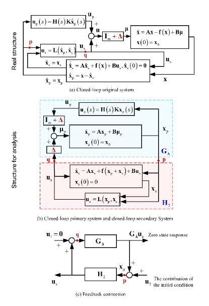
Figure 2: In the presence of unmodeled dynamics $\Delta\neq\mathbf{0}$, Fig. 2(a) shows the real closed-loop system corresponding to the original system, which can be transformed into Fig. 2(b) for analysis. Furthermore, Fig. 2(c) is an abstract feedback connection of Fig. 2(b).

By exploiting the interconnection structure and the small-gain theorem, the following theorem is drawn to prove the robust stability.

Theorem 2 For system (1) with $\Delta$ under Assumptions 1-2, suppose (i) Problems 1-2 are solved; (ii) the controller for system (1) with $\Delta=\mathbf{0}$ is designed as in (10); (iii) there exist $k_{l}>0$ such that $\left\|\mathbf{u}_{\text{s}}\right\|_{\mathcal{L_{\text{$2$}}}}\leq k_{l}\left\|\mathbf{x_{\text{p}}}\right\|_{\mathcal{L_{\text{$2$}}}}+\beta$, where , $\beta\in\mathcal{L}_{\text{$2$}}^{\text{$n$}}$ is a constant that depends on the initial state; (iv) $\mathbf{G}_{\Delta}$ is finite-gain $\mathcal{L}_{\text{$2$}}$ stable, namely $\mathbf{G}_{\Delta}:\mathcal{L}_{\text{$2$}}^{\text{$m$}}\rightarrow\mathcal{L}_{\text{$2$}}^{\text{$n$}}$ and

$$k_{l}\left\|\mathbf{G}_{\Delta}\right\|<1$$ (11)

where

$$\mathbf{G}_{\Delta}(s)=(s\mathbf{I}_{n}-\mathbf{A}-(\mathbf{I}_{m}+\Delta(s))\mathbf{H}(s)\mathbf{B}\mathbf{K})^{-1}\mathbf{B}\Delta(s).$$

Then, with controller (10), the state of system (1) satisfies $\mathbf{x}\in\mathcal{L}_{\text{$2$}}^{\text{$n$}}$.

Proof. On the one hand, Problem 2 for the secondary system is solved and

$$\left\|\mathbf{u}_{\text{s}}\right\|_{\mathcal{L_{\text{$2$}}}}\leq k_{l}\left\|\mathbf{x_{\text{p}}}\right\|_{\mathcal{L_{\text{$2$}}}}+\beta.$$ (12)

On the other hand, based on (8), (3), and (4), we have

$$\mathbf{x_{\text{p}}}=(s\mathbf{I}_{n}-\mathbf{A})^{-1}\mathbf{B}(\Delta\mathbf{u}_{\text{s}}+(\mathbf{I}_{m}+\Delta(s))\mathbf{H}(s)\mathbf{K}\mathbf{x_{\text{p}}})+(s\mathbf{I}_{n}-\mathbf{A})^{-1}\mathbf{x_{\text{0}}}.$$

Then, as shown in Fig. 2(c), we have

$$\mathbf{x_{\text{p}}}=\mathbf{G}_{\Delta}\mathbf{u}_{\text{s}}+\mathbf{u}_{\text{2}}$$ (13)

where $\mathbf{u}_{\text{2}}=(s\mathbf{I}_{n}-\mathbf{A}-(\mathbf{I}_{m}+\Delta(s))\mathbf{H}(s)\mathbf{B}\mathbf{K})^{-1}\mathbf{x_{\text{0}}}$. Since $\mathbf{G}_{\Delta}:\mathcal{L}_{\text{$2$}}^{\text{$m$}}\rightarrow\mathcal{L}_{\text{$2$}}^{\text{$n$}},\mathbf{u}_{\text{2}}\mathcal{\in L}_{\text{$2$}}^{\text{$n$}}$. Consequently,

$$\left\|\mathbf{x_{\text{p}}}\right\|_{\mathcal{L_{\text{$2$}}}}\leq\left\|\mathbf{G}_{\Delta}\right\|\left\|\mathbf{u}_{\text{s}}\right\|_{\mathcal{L_{\text{$2$}}}}+\left\|\mathbf{u}_{\text{2}}\right\|_{\mathcal{L_{\text{$2$}}}}.$$ (14)

Based on (12) and (14), if the condition (11) is satisfied, then the interconnection shown in Fig. 2(c) is finite-gain $\mathcal{L}_{\text{$2$}}$ stable with the input $\mathbf{u}=\left[\mathbf{u_{\text{1}}^{\text{T}}}\>\mathbf{u_{\text{2}}^{\text{T}}}\right]^{\text{T}}\in\mathcal{L}_{\text{$2$}}^{n+m}$ (see the small-gain theorem). Since $\mathbf{u}\in\mathcal{L}_{\text{$2$}}^{\text{$n+m$}},\mathbf{u}_{\text{s}}\mathcal{\in L}_{\text{$2$}}^{\text{$m$}}$ and $\mathbf{x_{\text{p}}}\in\mathcal{L}_{\text{$2$}}^{\text{$n$}}$. In addition, $\mathbf{x_{\text{s}}}\in\mathcal{L}_{\text{$2$}}^{\text{$n$}}$ can be guaranteed by Problem 2. Therefore, according to additive state decomposition, $\mathbf{x}\in\mathcal{L}_{\text{$2$}}^{\text{$n$}}$. $\Square$

With Theorem 2 in hand, we further have the following theorem for stability margin.

Theorem 3 (Stability Margin). For system (1) with $\Delta$ under Assumptions 1-2, suppose (i) Problems 1-2 are solved; (ii) the controller for system (1) with $\Delta=\mathbf{0}$ is designed as in (10). Then

(i) $\mathcal{L}_{\text{$2$}}$ gain margin of the closed-loop system, $\gamma_{\text{max}}>0$, is such that for any $\left|\gamma_{i}\right|\leq\gamma_{\text{max}}$, we have

$$k_{l}\left\|\mathbf{G}_{\gamma}\right\|<1$$ (15)

where $\mathbf{G}_{\gamma}(s)=(s\mathbf{I}_{n}-\mathbf{A}-(\mathbf{I}_{m}+\mathbf{E}_{1})\mathbf{H}(s)\mathbf{B}\mathbf{K})^{-1}\mathbf{B}\mathbf{E}_{1}$, $\mathbf{E}_{1}=\text{diag}\left(\gamma_{1},\gamma_{2},...,\gamma_{m}\right)$.

(ii) $\mathcal{L}_{\text{$2$}}$ time-delay margin of the closed-loop system, $\tau_{\text{max}}>0$, is such that for any $0\leq\tau_{i}\leq\tau_{\text{max}}$, we have

$$k_{l}\left\|\mathbf{G}_{\tau}\right\|<1$$ (16)

where $\mathbf{G}_{\tau}(s)=(s\mathbf{I}_{n}-\mathbf{A}-(\mathbf{I}_{m}+\text{$\mathbf{E}_{2}$})\mathbf{H}(s)\mathbf{B}\mathbf{K})^{-1}\mathbf{B}\mathbf{E}_{2}$, $\mathbf{E}_{2}=\text{diag$\left(\text{e}^{-s\tau_{1}}-1,...,\text{e}^{-s\tau_{m}}-1\right)$})$.

Proof. For the $\mathcal{L}_{\text{$2$}}$ gain margin, let $\Delta=\textrm{diag}\left(\gamma_{1},\gamma_{2},...,\gamma_{m}\right)$ in (2). Then, according to Theorem 2 and Definition 1, we can prove (i). Similarly, for the $\mathcal{L}_{\text{$2$}}$ time-delay margin, let $\Delta=\text{diag$\left(\text{e}^{-s\tau_{1}}-1,...,\text{e}^{-s\tau_{m}}-1\right)$}$ in (2). Then, according to Theorem 2 and Definition 1, we can prove (ii).$\Square$

IV-B Stability Margin Measurement

The $\mathcal{L}_{\text{$2$}}$ gain margin and $\mathcal{L}_{\text{$2$}}$ time-delay margin can be calculated theoretically according to the given parameters and Theorem 3. In the following, we will present a frequency-sweep method to acquire them. This offers a way to get the stability margin through real experiments rather than theoretical calculation, which approaches reality more.

IV-B1 Stability Margin for the Primary System

We first should find $\gamma_{\text{max,1}}$ and $\tau_{\text{max,1}}$ to make $\mathbf{G}_{\Delta}:\mathcal{L}_{\text{$2$}}^{\text{$m$}}\rightarrow\mathcal{L}_{\text{$2$}}^{\text{$n$}}$, namely the stability condition for the primary system (the upper half part of the system shown in Fig. 4(b)). Because the primary system is linear, the proposed stability margin analysis method in [20]can be used. The stability margin is obtained by measuring the upper half part of the system shown in Fig. 4(b). For SISO systems, the classic stability margin is considered; for MIMO systems, the $\mathcal{L_{\text{$2$}}}$ stability margin is considered.

IV-B2 Stability Margin for the Whole System

Based on the results above, we should further find $\gamma_{\text{max,2}}$ and $\tau_{\text{max,2}}$ to make $k_{l}\left\|\mathbf{G}_{\Delta}\right\|<1$, namely the stability condition for the whole system.

For the $\mathcal{L}_{\text{$2$}}$ gain margin, according to $\left(\ref{eq:Gain}\right)$, if

$$\gamma_{\text{max,2}}<\left\|\mathbf{G}_{0}\mathbf{B}\right\|^{-1}\left(k_{l}\right)^{-1}$$

then $\gamma\in\left[-\gamma_{\text{max,2}},\>\gamma_{\text{max,2}}\right]$ can make $k_{l}\left\|\mathbf{G}_{\gamma}\right\|<1$. Here

$$\gamma_{\text{max,2}}=\left(1-\varepsilon_{3}\right)\left\|\mathbf{G}_{0}\mathbf{B}\right\|^{-1}\left(k_{l}\right)^{-1}$$ (17)

where $0<\varepsilon_{3}<1$ is often chosen sufficiently small. For the $\mathcal{L}_{\text{$2$}}$ time-delay margin, we have

$$\tau_{\text{max,2}}<\left\|s\mathbf{G}_{0}\mathbf{B}\right\|^{-1}\left(k_{l}\right)^{-1}$$

then $\tau\in\left[0,\>\tau_{\text{max,2}}\right]$ can make $k_{l}\left\|\mathbf{G}_{\tau}\right\|<1$. Here

$$\tau_{\text{max,2}}=\left(1-\varepsilon_{4}\right)\left\|s\mathbf{G}_{0}\mathbf{B}\right\|^{-1}\left(k_{l}\right)^{-1}$$ (18)

where $0<\varepsilon_{4}<1$ is often chosen sufficiently small.

In the following, we aim to get $\left\|\mathbf{G}_{0}\mathbf{B}\right\|$ and $\left\|s\mathbf{G}_{0}\mathbf{B}\right\|$ by the frequency-sweep method. To obtain $\mathbf{G}_{0}\mathbf{B}$, we should modify Fig. 2 to be Fig. 3. In Fig. 3, the open loops from $\mathbf{q}^{\prime\prime}$ to $\mathbf{p}$ for Fig. 3(a) (real structure) and Fig. 3(b) (structure for analysis) are the same. In Fig. 3(b), the transfer function from $\mathbf{q}^{\prime\prime}$ to $\mathbf{p}$ is $\mathbf{G}_{0}\mathbf{B}$. The frequency-sweep method is only applicable to the open loop from $\mathbf{q}^{\prime\prime}$ to $\mathbf{p}$ in Fig. 3(a), because the open loop in Fig. 3(b) is conceived only for controller design and analysis. The procedure to get $\mathbf{G}_{0}\mathbf{B}$ is as follows:

• Recalling the system with $\Delta$ as shown in Fig. 2(b), it can be seen that the terms $\Delta$ and $\mathbf{I}_{m}+\Delta$ will make an obstacle to obtaining $\mathbf{G}_{0}\mathbf{B}$ from $\mathbf{q}$ to $\mathbf{p}$.

• Let $\Delta=\mathbf{I}_{m}$ and insert a gain matrix $1/2\mathbf{I}_{m}$ into the closed-loop primary system in Fig. 2(b). Then, in practice, $\mathbf{G}_{0}\mathbf{B}$ is obtained from $\mathbf{q}^{\prime\prime}$ to $\mathbf{p}$ in the way shown in Fig. 3(a).

It should be noticed that these additional terms are only used to obtain $\mathbf{G}_{0}\mathbf{B}$, where $\Delta=\mathbf{I}_{m}$ is a simple way to establish $\mathbf{G}_{0}\mathbf{B}$.

As shown in Fig. 3(b), the output responses are collected at the point $\mathbf{p}$ by feeding frequency-sweep inputs (sweeping the frequency of input signals from 0 to a value just beyond the frequency range of the system) to the system at the point $\mathbf{q}^{\prime\prime}$ . Based on the input-output data, one can get $\left\|\mathbf{G}_{0}\mathbf{B}\right\|$ and $\left\|s\mathbf{G}_{0}\mathbf{B}\right\|$. After getting $\left\|\mathbf{G}_{0}\mathbf{B}\right\|$ and $\left\|s\mathbf{G}_{0}\mathbf{B}\right\|$ by the frequency-sweep method, $\gamma_{\text{max,2}}$ and $\tau_{\text{max,2}}$ can be obtained by (17), (18), namely the stability condition for the whole system is determined.

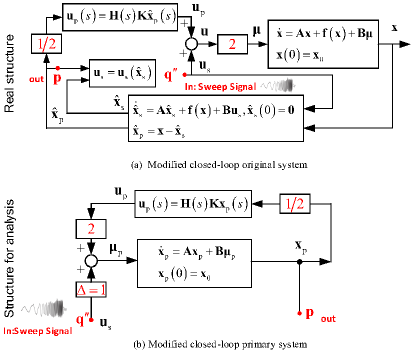
Figure 3: Establishing $\mathbf{G}_{0}\mathbf{B}$. From the input-output perspective, the open-loop systems from $\mathbf{q}^{\prime\prime}$ to $\mathbf{p}$ in Fig. 3(a) and Fig. 3(b) are equivalent.

IV-B3 Stability Margin

Finally, with $\gamma_{\text{max,1}}$, $\tau_{\text{max,1}}$, $\gamma_{\text{max,2}}$ and $\tau_{\text{max,2}}$ available, the $\mathcal{L}_{\text{$2$}}$ gain margin is

$$\gamma_{\text{max}}\thickapprox\min\left(\gamma_{\text{max,1}},\gamma_{\text{max,2}}\right)$$

and the $\mathcal{L}_{\text{$2$}}$ time-delay margin is

$$\tau_{\text{max}}\thickapprox\min\left(\tau_{\text{max,1}},\tau_{\text{max,2}}\right).$$

IV-C Whole Design and Analysis Procedure

The complete procedure to design the controller and measure the stability margin is summarized in Fig. 4. The procedure consists of three steps, in which Step (a) belongs to the state-compensation-linearization-based control design (corresponding to Section III); Step (b) works for the stability margin measurement for the primary system (corresponding to Section IV-B1); Step (c) aims to measure the stability margin for the whole system (corresponding to Section IV-B2). This approach has the advantage of getting stability margin through data by real experiments, which takes both model uncertainties and external disturbances into account, and thus approaches to practice more.

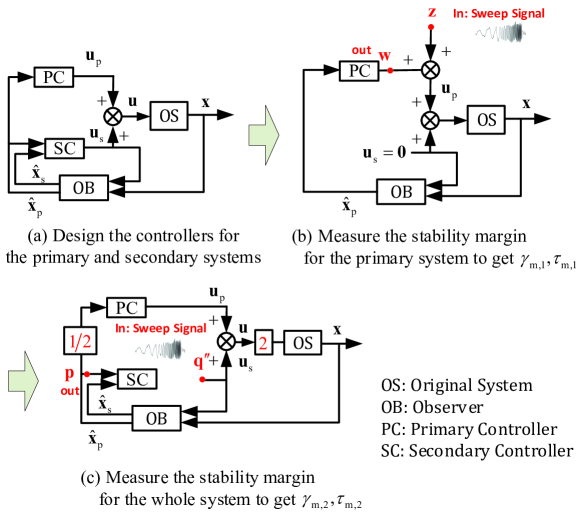
Figure 4: Procedure to design the controller and measure the stability margin.

V Simulation Studies

In order to show the effectiveness of the state-compensation-linearization-based stability margin analysis method proposed above, three illustrative examples are considered in the simulation.

V-A Example 1: An SISO nonlinear system

This example aims to demonstrate the complete procedure to design the controller and measure the stability margin for an SISO nonlinear system by using the proposed method, and to show the difference between the defined stability margin and the classic frequency-domain stability margin. Consider the following second-order nonlinear system

$$\dot{x}_{1} =x_{2}$$

$$\dot{x}_{2} =-2x_{1}-3x_{2}+\frac{x_{2}^{2}}{1+ax_{2}^{2}}+\mu$$ (19)

with

$$\mu=\left(1+\Delta\right)u$$

where $a>0$. The system can be transformed into the form in (1) with

$$\mathbf{A=}\left[\begin{array}[]{cc}0&1\\ -2&-3\end{array}\right],\mathbf{f}\left(\mathbf{x}\right)=\left[\begin{array}[]{c}0\\ \frac{x_{2}^{2}}{1+ax_{2}^{2}}\end{array}\right],\mathbf{b}=\left[\begin{array}[]{c}0\\ 1\end{array}\right].$$

It is obvious that $\mathbf{A}$ is stable.

V-A1 State-compensation-linearization-based control (SCLC)

In this part, the controller design and stability margin analysis will be carried out by following the procedure illustrated in Fig. 4.

$\bullet$ Step (a). Design controllers for the primary system and the secondary system. For the controller (8), the LQR method is employed to calculate the feedback matrix $\mathbf{k}$. Besides, let $h\left(s\right)=1$. Then, the primary controller follows

$$u_{\text{p}}=\mathbf{k}^{\text{T}}\mathbf{\hat{x}}_{\text{p}}.$$

For the controller (9), the backstepping control is adopted, and a secondary controller is designed as

$$u_{\text{s}}=\left(3-c_{1}-c_{2}\right)\hat{x}_{\text{s},2}+\left(1-c_{1}c_{2}\right)\hat{x}_{\text{s},1}-\frac{(\hat{x}_{\text{p},2}+\hat{x}_{\text{s},2})^{2}}{1+a(\hat{x}_{\text{p},2}+\hat{x}_{\text{s},2})^{2}}$$ (20)

where $c_{1},c_{2}>0$ are parameters to be specified later. The concrete design procedure for backstepping control is omitted here for it is straightforward by routine steps.

$\bullet$ Step (b). Measure the stability margin for the primary system to get $\gamma_{\text{max},1}$ and $\tau_{\text{max},1}$. Because the primary system is an SISO system, the classic stability margin can be considered. The frequency-sweep method is utilized here. Based on the input-output data, the Bode plot of the open-loop system is obtained. Then, the GM $G_{\text{m},1}$, the PM $P_{\text{m},1}$, and the gain and phase crossover frequencies $\omega_{\text{cg},1},\omega_{\text{cp},1}$ are obtained relying on the Bode plot. Finally, $\gamma_{\text{max},1}$ and $\tau_{\text{max},1}$ are determined.

$\bullet$ Step (c). Measure the stability margin for the whole system to get $\gamma_{\text{max},2}$ and $\tau_{\text{max},2}$. First, $k_{l}$ is calculated based on (20). Then, based on Section IV-B2, the frequency-sweep test is carried out by applying frequency-sweep input signals to the system at the point $\mathbf{q}^{\prime\prime}$ and collecting output responses at the point $\mathbf{p}$, as shown in Fig. 4(c). By the corresponding collected input-output data, $\left\|\mathbf{G}_{0}\mathbf{b}\right\|$ and $\left\|s\mathbf{G}_{0}\mathbf{b}\right\|$ are gotten, and then $\gamma_{\text{max},2}$ and $\tau_{\text{max},2}$ are obtained by (17) and (18).

V-A2 JLC for comparison

A commonly-used way is to apply linear control techniques at discrete operating points within the operating envelope, and then the classic frequency-domain stability margin is used to evaluate the designed controllers at these discrete points. For stabilizing control, the operating point is the equilibrium point, namely, the origin herein. By linearizing the system (19) at the origin $\mathbf{x}=\mathbf{0}$, one has

$$\dot{x}_{1} =x_{2}$$

$$\dot{x}_{2} =-2x_{1}-3x_{2}+\mu.$$ (21)

Then, similar to the controller (8), an LQR-based stabilizing controller for (21) is designed as

$$u=\mathbf{k}^{\text{T}}\mathbf{x.}$$ (22)

where the parameter $\mathbf{k}$ is chosen the same as the state-compensation-linearization-based control mentioned above.

The stability margin analysis for the closed-loop system consisting of (21) and (22) can be done by a classic frequency-domain method, which is the same as that of the primary system in the state-compensation-linearization-based control.

V-A3 Simulation results

For a fair comparison, the parameters in LQR are selected as the same values for SCLC and JLC. In the following simulations, $\mathbf{Q}=$diag$\left(1\text{, }1\right),R=1$ are selected, resulting in $\mathbf{k=-}\left[0.236\text{ }0.236\right]^{\text{T}}$. Besides, let $a=0.01,\mathbf{x}_{0}=[10$ $10]^{\text{T}},c_{1},c_{2}=20$. The corresponding stabilizing control performance is compared in Fig. 5. It can be observed that SCLC outperforms JLC.

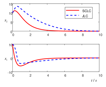
Figure 5: State response (Example 2).

In the following, the stability margin analysis is performed after the stabilizing control has been done. For SCLC, the stability margin for the primary system is studied firstly. The GM and the PM are obtained as $G_{\text{m},1}=\infty$, $P_{\text{m},1}=\infty$ by the Bode plot as represented in Fig. 6(a), which comes from the frequency-sweep test. Then, it is determined that $\gamma_{\text{max},1}=\infty$ and $\tau_{\text{max},1}=\infty$. Thus, the primary system is stable, i.e., $\mathbf{G}_{\Delta}$: $\mathcal{L}_{2}^{1}\rightarrow\mathcal{L}_{2}^{n}$, and has a large stability margin. Then, the stability margin for the whole system is obtained in two ways: the theoretical computation method and the frequency-sweep method. The theoretical computation method is to find $\gamma_{\text{max},2}$ and $\tau_{\text{max},2}$ by gradually increasing them from $0$ until the inequality (11) does not hold. On the other hand, the frequency-sweep method is to get $\left\|\mathbf{G}_{0}\mathbf{b}\right\|$ and $\left\|s\mathbf{G}_{0}\mathbf{b}\right\|$ by the corresponding frequency-sweep data, and then $\gamma_{\text{max},2}$ and $\tau_{\text{max},2}$ can be obtained by equations (17), (18). Through theoretical computation, the stability margin for the whole system is obtained as $\gamma_{\text{max},2}=0.428$ and $\tau_{\text{max},2}=0.22$, while through the frequency-sweep method, it is obtained that $\gamma_{\text{max},2}=0.45$ and $\tau_{\text{max},2}=0.20$. Note that the two groups of results show good agreement with each other. Finally, $\gamma_{\text{max}}\approx\min\left(\gamma_{\text{max},1},\gamma_{\text{max},2}\right)=0.45$, $\tau_{\text{max}}\approx\min\left(\tau_{\text{max},1},\tau_{\text{max},2}\right)=0.20$.

To verify the obtained $\gamma_{\text{max}}$, $\Delta=0.45$ is added to the original system, and the corresponding state response is depicted in Fig. 6(b). To verify the obtained $\tau_{\text{max}}$, $\Delta=e^{-0.2s}-1$ is added to the original system, and the corresponding state response is depicted in Fig. 6(c). It can be observed that although the state responses all get worse compared to the results in Fig. 5, the system is still stable eventually.

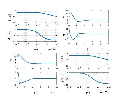
Figure 6: Stability margin analysis results (Example 2): (a) Bode plot for the primary system in SCLC; (b) Validation test results of $\gamma_{\text{max}}$; (c) Validation test results of $\tau_{\text{max}}$; (d) Bode plot in JLC.

For JLC, the current practice is to certify such systems by the GM and PM at the origin. From Fig. 6(d), the GM and PM are $G_{\text{m}}=\infty$, $P_{\text{m}}=\infty,$ which are nearly the same as the obtained stability margin results for the primary system in SCLC. Actually, the method directly treats the nonlinear system as a linear one, and the obtained stability margin is just the stability margin of the corresponding linearized system, which may be inaccurate when the nonlinearity is strong, or the system state is far away from the operating point.

V-B Example 2: An SISO strongly nonlinear system

This example aims to verify that the obtained classic frequency-domain stability margin may be unreliable when the assumption of weak nonlinearity fails. A strongly nonlinear system is considered

$$\dot{x}_{1} =x_{1}+x_{2}$$

$$\dot{x}_{2} =x_{2}+x_{2}^{2}+\mu.$$ (23)

Its state-space realization is of the form (1) with

$$\mathbf{A=}\left[\begin{array}[]{cc}1&1\\ 0&1\end{array}\right],f\left(\mathbf{x}\right)=\left[\begin{array}[]{c}0\\ x_{2}^{2}\end{array}\right],\mathbf{b}=\left[\begin{array}[]{c}0\\ 1\end{array}\right].$$

Notice that $\mathbf{A}$ is unstable, but $\left(\mathbf{A},\mathbf{b}\right)$ is controllable. Thus, a state feedback controller is designed firstly to obtain a stable $\mathbf{\bar{A}=A-bk}_{0}^{\text{T}}$. Then, the subsequent stabilizing controller design is similar to that of Example 1 and omitted here.

First, choose $\mathbf{k}_{0}=\left[6\text{ }5\right]^{\text{T}}$ to obtain a stable $\mathbf{\bar{A}}$. Then, for a fair comparison, the parameters in LQR are selected as the same values for the state-compensation-linearization-based control and JLC. In the following simulations, $\mathbf{Q}=$diag$\left(10\text{,}10\right),R=1$ are selected resulting in $\mathbf{k=-}\left[4.88\text{ }1.98\right]^{\text{T}}$. Besides, let $c_{1},c_{2}=20$. When the initial state value is set to $\mathbf{x}_{0}=[3$ $3]^{\text{T}},$ the state response is depicted in Fig. 7(a), which shows that SCLC has a faster state convergence rate than JLC. Furthermore, when the initial state is changed to $\mathbf{x}_{0}=[4$ $4]^{\text{T}}$, it can be found from Fig. 7(b) that system divergence occurs for JLC, while SCLC still performs well.

For JLC, the calculated stability margin is $G_{\text{m}}=\infty$, $P_{\text{m}}=\infty$. However, the instability phenomenon occurs when the initial state is $\mathbf{x}_{0}=[4$ $4]^{\text{T}}$. Hence, it convincingly shows that the classic stability margin is unreliable in this case. The reason is that the closed-loop system is still nonlinear, and the calculated stability margin is just valid in a small neighborhood of the selected operating point (the point where the system is linearized).

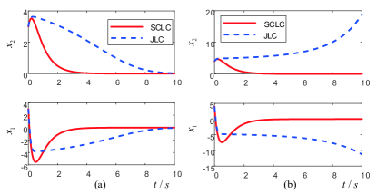
Figure 7: State response (Example 3): (a) $\mathbf{x}_{0}=[3$ $3]^{\text{T}}$; (b) $\mathbf{x}_{0}=[4$ $4]^{\text{T}}$.

V-C Example 3: An MIMO nonlinear system

This example aims to demonstrate the complete procedure to design the controller and measure the stability margin for a MIMO nonlinear system by using the proposed method, and to show the difference between the defined stability margin and the classic frequency-domain stability margin. Consider a two-input two-output nonlinear system of the form in (1) with

$$\mathbf{A} =\left[\begin{array}[]{ccc}-1&0&1\\ 0&-1&1\\ 0&-2&-3\end{array}\right],\mathbf{B}=\left[\begin{array}[]{cc}0&-1\\ 0&1\\ 1&1\end{array}\right],$$ (30)

$$\mathbf{f}\left(\mathbf{x}\right)=\left[\begin{array}[]{c}0\\ 0\\ x_{3}^{2}\frac{1}{1+ax_{3}^{2}}\end{array}\right].$$ (34)

where $\mathbf{x}=\left[x_{1}x_{2}x_{3}\right]^{\text{T}}$. It can be verified that $\mathbf{A}$ is a Hurwitz matrix.

V-C1 State-compensation-linearization-based control

In this part, the controller design and stability margin analysis will be carried out by following the procedure illustrated in Fig. 4.

$\bullet$ Step (a). Design controllers for the primary system and the secondary system. For the controller (8), the LQR method is employed to calculate the feedback matrix $\mathbf{K}$. Besides, let $\mathbf{H}(s)=\mathbf{I}_{m}$. Then, the primary controller follows

$$\mathbf{u}_{\text{p}}=\mathbf{K}\mathbf{\hat{x}_{\text{p}}}.$$

For the controller (9), the Lyapunov method is adopted, and a secondary controller is designed as

$$\mathbf{u}_{\text{s}}=\left[\begin{array}[]{c}-\left(x_{\text{s},1}-x_{\text{s},2}+\left(x_{\text{s},3}+x_{\text{p},3}\right)^{2}\frac{1}{1+a\left(x_{\text{s},3}+x_{\text{p},3}\right)^{2}}\right)\\ -c\left(-x_{\text{s},1}+x_{\text{s},2}+x_{\text{s},3}\right)\end{array}\right]$$ (35)

where $c>0$ is the controller parameter to be specified later. The Lyapunov design procedure is routine, and hence omitted here.

$\bullet$ Step (b). Measure the stability margin for the primary system to get $\gamma_{\text{max,1}}$ and $\tau_{\text{max,1}}$. Because the primary system is a MIMO linear system, the proposed $\mathcal{L_{\text{$2$}}}$ stability margin in [20] can be considered.

$\bullet$ Step (c). Measure the stability margin for the whole system to get $\gamma_{\text{max,2}}$ and $\tau_{\text{max,2}}$. First, $k_{l}$ is calculated based on (35). Then, based on Section IV-B2, the frequency-sweep test is carried out by applying frequency-sweep input signals to the system at the point $\mathbf{q}^{\prime\prime}$ and collecting output responses at the point $\mathbf{p}$, as shown in Fig. 4(c). Based on the collected input-output data, $\left\|\mathbf{G}_{0}\mathbf{B}\right\|$ and $\left\|s\mathbf{G}_{0}\mathbf{B}\right\|$ are obtained, and then $\gamma_{\text{max,2}}$ and $\tau_{\text{max,2}}$ are gotten by (17) and (18).

V-C2 JLC for comparison

A commonly-used way is to apply linear control techniques at discrete operating points within the operating envelope, and then classic frequency-domain stability margin is used to evaluate the designed controllers at the discrete points. For stabilizing control, the operating point is the equilibrium point, i.e., the origin herein. By linearizing the system (30) at the origin $\mathbf{x}=\mathbf{0}$, one has

$$\dot{\mathbf{x}}=\mathbf{Ax}+\mathbf{Bu.}$$ (36)

Then, similar to the controller (8), an LQR-based stabilizing controller for (36) is designed as

$$\mathbf{u}=\mathbf{K}\mathbf{x}.$$ (37)

Through neglecting the coupling among loops, the stability margin analysis for the closed-loop system consisting of (36) and (37) can be done by classic frequency-domain stability margin. In practice, the Bode plot is obtained by the frequency-sweep technique, by which the resulting stability margin is obtained.

V-C3 Simulation results

For a fair comparison, the parameters in LQR are selected as the same values for state-compensation-linearization-based control and JLC. In the following simulations, $\mathbf{Q}=\text{diag$\left(1,1,1\right)$},\mathbf{R}=\text{diag}\left(1,1\right)$ are selected. Besides, let $a=0.01,\mathbf{x_{0}}=\left[10\>10\>10\right]^{\text{T}},c=5$.

Stability margin analysis is performed after the stabilizing control has been done. For state-compensation-linearization-based control, the stability margin for the primary system is investigated firstly. The stability margin is obtained in two ways: the theoretical computation method and the frequency-sweep method. Through theoretical computation, the stability margin for the primary system is obtained as $\gamma_{\text{max,1}}=2.262$ and $\tau_{\text{max,1}}=1.134$, while through the frequency-sweep method, it is acquired that $\gamma_{\text{max,1}}=2.261$ and $\tau_{\text{max,1}}=1.134$. Thus, the primary system is stable, i.e., $\mathbf{G}_{\Delta}:\mathcal{L}_{\text{$2$}}^{\text{$m$}}\rightarrow\mathcal{L}_{\text{$2$}}^{\text{$n$}}$.

Then, the stability margin for the whole system is also obtained in the mentioned two ways. Through theoretical computation, the stability margin for the whole system is obtained as $\gamma_{\text{max,2}}=0.17$ and $\tau_{\text{max,2}}=0.08$, while through the frequency-sweep method, it is obtained that $\gamma_{\text{max,2}}=0.19$ and $\tau_{\text{max,2}}=0.08$. Note that the two groups of results show a good agreement with each other. Finally, $\gamma_{\text{max}}\thickapprox\min\left(\gamma_{\text{max,1}},\gamma_{\text{max,2}}\right)=0.19$, $\tau_{\text{max}}\thickapprox\min\left(\tau_{\text{max,1}},\tau_{\text{max,2}}\right)=0.08$.

To verify the obtained $\gamma_{\text{max}}$, $\Delta=\text{diag$\left(0.19,0.19\right)$ }$ is added to the original system, and the corresponding state response is depicted in Fig. 8(a). To verify the obtained $\tau_{\text{max}}$, $\Delta=\textrm{diag}\left(e^{-0.08s}-1,e^{-0.08s}-1\right)$ is added to the original system, and the corresponding state response is depicted in Fig. 8(b). It can be observed that the system is still stable.

For JLC, the current practice is to certify such systems by the GM and PM at the origin. There are two loops for the considered system. From Fig. 8(c),(d), the GM and PM for the two loops are $G_{\text{m}}=\infty,P_{\text{m}}=\infty$. Actually, the method directly treats the nonlinear system as a linear one, and the obtained stability margin is just the stability margin of the corresponding linearized system. Moreover, the coupling between the two loops is neglected, and each loop is considered individually. The obtained stability margin may be inaccurate when coupling or nonlinearity is strong, or the system state is far away from the operating point.

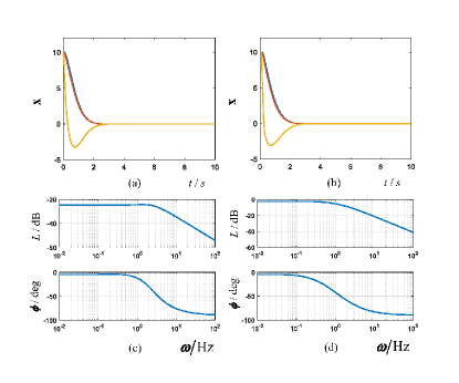
Figure 8: stability margin analysis results (Example 4): (a) Validation test results of $\gamma_{\text{max}}$; (b) Validation test results of $\tau_{\text{max}}$; (c) Bode plot of the first loop in JLC; (d) Bode plot of the second loop in JLC.

V-D Discussions

From the simulation results of the three illustrative examples, it can be seen that the state-compensation-linearization-based stabilizing control and stability margin analysis outperforms the traditional stabilizing control and stability margin analysis in two aspects. First, compared with JLC and FLC, the stabilizing control performance of state-compensation-linearization-based control is better. State-compensation-linearization-based control can achieve a higher state convergence rate and avoid the uncontrollability of JLC and the singularity of FLC. Secondly, the subsequent stability margin analysis can make the classical frequency-domain stability margin available for nonlinear systems. The classical frequency-domain stability margin may be insufficient when it is applied to nonlinear systems directly owing to the nonlinearity. However, it can work well under the proposed state-compensation-linearization-based control framework by utilizing the small-gain theorem. What is more, a frequency-domain series compensator, namely $\mathbf{H}\left(s\right)$ in the controller (8) can be introduced additionally to pursue a better stability margin when the actual stability margin is unsatisfactory.

VI Conclusions

Based on the state-compensation-linearization-based stabilizing control, the paper focuses on the stability margin analysis for nonlinear systems. The $\mathcal{L}_{2}$ gain margin and $\mathcal{L}_{2}$ time-delay margin for the closed-loop nonlinear system are defined, and derived by the small-gain theorem. The stability margin measurement depends on the frequency-sweep method. Three examples are provided to show the concrete design and analysis procedure. Simulation results illustrate that the state-compensation-linearization-based control outperforms Jacobian linearization based control and feedback linearization based control to some extent. It should be noted that the frequency-domain stability margin analysis is extended smoothly to nonlinear systems. As a result, it is supposed to be of interest to many engineers.

References

- [1] K. Zhou, J. C. Doyle, K. Glover et al., Robust and optimal control, vol. 40. Englewood Cliffs, NJ, USA: Prentice hall, 1996.
- [2] R. C. Dorf and R. H. Bishop, Modern control systems. Upper Saddle River, NJ, USA: Pearson (Addison-Wesley), 2011.
- [3] M. Lichter, A. Bateman, and G. Balas, “Flight test evaluation of a run-time stability margin estimation tool,” in AIAA Guidance, Navigation, and Control Conference, ser. AIAA Paper 2009-6257, 2009.
- [4] W. K. Ho, O. Gan, E. B. Tay, and E. Ang, “Performance and gain and phase margins of well-known PID tuning formulas,” IEEE Transactions on Control Systems Technology, vol. 4, no. 4, pp. 473–477, 1996.
- [5] K. K. Tan, Q.-G. Wang, and C. C. Hang, Advances in PID control. Berlin, Germany: Springer Science & Business Media, 2012.
- [6] J.-R. Ren and Q. Quan, “Initial research on stability margin of nonlinear systems under additive-state-decomposition-based control framework,” in 2016 Chinese Control and Decision Conference (CCDC), pp. 5766–5771. IEEE, 2016.
- [7] I. M. Horowitz, Synthesis of feedback systems. Amsterdam, Netherlands: Elsevier, 2013.
- [8] Y. Kim, “On the stability margin of networked dynamical systems,” IEEE Transactions on Automatic Control, vol. 62, no. 10, pp. 5451–5456, 2017.
- [9] M. French, “Adaptive control and robustness in the gap metric,” IEEE Transactions on Automatic Control, vol. 53, no. 2, pp. 461–478, 2008.
- [10] P. Konghuayrob and S. Kaitwanidvilai, “Low order robust -gap metric loop shaping controller synthesis based on particle swarm optimization,” International Journal of Innovative Computing, Information and Control, vol. 13, no. 6, pp. 1777–1789, 2017.
- [11] M. Bozorg and E. J. Davison, “Control of time delay processes with uncertain delays: Time delay stability margins,” Journal of Process Control, vol. 16, no. 4, pp. 403–408, 2006.
- [12] F. Todeschini, M. Corno, G. Panzani, S. Fiorenti, and S. M. Savaresi, “Adaptive cascade control of a brake-by-wire actuator for sport motorcycles,” IEEE/ASME Transactions on Mechatronics, vol. 20, no. 3, pp. 1310–1319, 2015.
- [13] J. Li, X. Qi, Y. Xia, F. Pu, and K. Chang, “Frequency domain stability analysis of nonlinear active disturbance rejection control system,” ISA transactions, vol. 56, pp. 188–195, 2015.
- [14] H. K. Khalil, Nonlinear systems. Englewood Cliffs, NJ, USA: Prentice hall, 2002.
- [15] X. Yang, J. J. Zhu, and A. S. Hodel, “Singular perturbation margin and generalised gain margin for linear time-invariant systems,” International Journal of Control, vol. 88, no. 1, pp. 11–29, 2015.
- [16] V. Chellaboina and W. M. Haddad, “Stability margins of nonlinear optimal regulators with nonquadratic performance criteria involving cross-weighting terms,” Systems & control letters, vol. 39, no. 1, pp. 71–78, 2000.
- [17] C. K. Ahn and M. K. Song, “New results on stability margins of nonlinear discrete-time receding horizon control,” International Journal of Innovative Computing, Information and Control, vol. 9, no. 4, pp. 1703–1713, 2013.
- [18] C. Regan, “In-flight stability analysis of the X-48B aircraft,” in AIAA atmospheric flight mechanics conference and exhibit, ser. AIAA Paper 2009-6571, 2008.
- [19] Q. Quan and J. Ren, “State compensation linearization and control,” arXiv preprint arXiv:2406.00285, 2024.
- [20] J. Ren, Q. Quan, B. Xu, S. Wang, and K.-Y. Cai, “Data-driven stability margin for linear multivariable systems,” International Journal of Robust and Nonlinear Control, vol. n/a, DOI https://doi.org/10.1002/rnc.7413, no. n/a. [Online]. Available: https://onlinelibrary.wiley.com/doi/abs/10.1002/rnc.7413