Learning $k$-Determinantal Point Processes for
Personalized Ranking

Abstract

The key to personalized recommendation is to predict a personalized ranking on a catalog of items by modeling the user’s preferences. There are many personalized ranking approaches for item recommendation from implicit feedback like Bayesian Personalized Ranking (BPR) and listwise ranking. Despite these methods have shown performance benefits, there are still limitations affecting recommendation performance. First, none of them directly optimize ranking of sets, causing inadequate exploitation of correlations among multiple items. Second, the diversity aspect of recommendations is insufficiently addressed compared to relevance.

In this work, we present a new optimization criterion L$k$P based on set probability comparison for personalized ranking that moves beyond traditional ranking-based methods. It formalizes set-level relevance and diversity ranking comparisons through a Determinantal Point Process (DPP) kernel decomposition. To confer ranking interpretability to the DPP set probabilities and prioritize the practicality of L$k$P, we condition the standard DPP on the cardinality $k$ of the DPP-distributed set, known as $k$-DPP, a less-explored extension of DPP. The generic stochastic gradient descent based technique can be directly applied to optimizing models that employ L$k$P. We implement L$k$P in the context of both Matrix Factorization (MF) and neural networks approaches, on three real-world datasets, obtaining improved relevance and diversity performances. L$k$P is broadly applicable, and when applied to existing recommendation models it also yields strong performance improvements, suggesting that L$k$P holds significant value to the field of recommender systems.

I Introduction

Recommender systems are ubiquitous services in many online platforms including social media and e-commerce, and play a crucial role in alleviating information overload by efficiently anticipating user preferences. This work focuses on item recommendation [1, 2], wherein the task involves generating a personalized ranking of items based on the user’s observed interactions with the system. In real-world scenarios, implicit feedback, such as clicks and views, is more readily available and collected compared to explicit feedback, e.g., ratings and reviews, making it a valuable resource for understanding user preferences.

To guide recommendation models in learning user preferences from implicit feedback, optimization objectives play a crucial role. One commonly used approach involves pointwise loss functions, e.g., binary cross entropy and squared error, which measure the discrepancy between the model’s predicted preference scores and the actual labels on an individual instance basis. Given that the goal of item recommendation is to provide a personalized ranking list to a specific user, it naturally leads to the adoption of ranking-based optimization methods. Among these, the popular pairwise ranking approach, BPR [1], assumes that an observed item ranks higher than a randomly selected unobserved (negative) item from the perspective of a specific user. Listwise ranking methods usually maximize the probability of permutation of the target list [3, 4]. In recent years, some studies have attempted to bring the correlation within items into ranking-based optimization, leading to the topic of setwise ranking. Two eminent and state-of-the-art set-based ranking methods are SetRank [5] and Set2SetRank [6]. SetRank encourages an observed item to rank in front of multiple unobserved items in each list by making use of the concept of permutation probability. Set2SetRank models the set ranking based on item to item comparison and summarization of distance measurements between items.

However, there are remain two problems in existing approaches: (i) Structure information and correlations are far from well exploited and modeled. As shown in the upper layer of Figure 1, the correlations among items are fully ignored by pointwise and pairwise learning; listwise-based models center solely on the order correlation in the ranking list of items, while the binary nature of implicit feedback obstructs the acquisition of clear order correlations; the recently proposed setwise ranking optimization models (e.g., SetRank and Set2SetRank) intend to construct set-level comparisons, but are still confined to a BPR optimization criterion, and the set ranking is obtained by summarizing the individual items in each set, rather than recognizing multiple items as a whole (i.e. set) that they are in order to more meaningfully compare them. Taking implicit feedback in Figure 1 as an illustration, a ranking optimization, which treats entire sets as cohesive entities for comparison (concrete set-level optimization), not only enables us to model explicit ranking comparisons, such as $\left\{v_{3}^{(1)},v_{6}^{(1)},v_{8}^{(1)}\right\}>_{u}\left\{v_{4}^{(0)},v_{5}^{(0)},v_{9}^{(0)}\right\}$ (superscripts $1$ and $0$ denote observed and unobserved items, respectively), but also to discern subtle preferences, such as the greater potential interest of item $v_{4}^{(0)}$ over $v_{5}^{(0)}$ in $\left\{v_{3}^{(1)},v_{6}^{(1)},v_{4}^{(0)}\right\}>_{u}\left\{v_{3}^{(1)},v_{6}^{(1)},v_{5}^{(0)}\right\}$ and the stronger dependency of $v_{8}^{1}$ with $v_{3}^{(1)}$ and $v_{6}^{(1)}$ compared to $v_{10}^{(1)}$ in $\left\{v_{3}^{(1)},v_{6}^{(1)},v_{8}^{(1)}\right\}>_{u}\left\{v_{3}^{(1)},v_{6}^{(1)},v_{10}^{(1)}\right\}$. This implies that the concrete set-level optimization criterion offers a wide range of potential combinations and aids in capturing intricate dependency relationships; (ii) The objective of diversifying recommendations to mine additional interests for users, is not involved in existing optimization criterion approaches. Consequently, item recommendation models that employ these optimization objectives tend to favor popular and rather relevant items (often already known by users) [7, 8], but lose sight of raising the ranking of diversified results for broadening users’ horizons.

To overcome these limitations, this work introduces a concrete set-level optimization criterion that facilitates ranking optimization through a direct comparison of different sets’ probabilities of being a $k$-DPP. Here, $k$-DPP refers to a less-explored extension of the well-established concept, Determinantal Point Process (DPP). By leveraging the balance-focused quality vs. diversity decomposition of the DPP kernel, we are able to seamlessly integrate two types of ranking comparison (i.e., relevance comparison and diversity comparison), thus offering a comprehensive measure of sets. The motivation for employing $k$-DPP lies in its ability to add ranking interpretability to DPP set probabilities, making them practically useful for achieving optimal recommendation sets. We name the proposed optimization criterion as L$k$P, an acronym underlining its aim to learn probabilities of specific subsets under the tailored $k$-DPP distribution. L$k$P presents an effective solution that acknowledges item correlations and diversity, thereby delivering an advanced recommendation model that boosts accuracy and diversity.

We summarize the contributions of this work as follows:

• We propose a concrete set-level optimization criterion, named L$k$P, that advances ranking optimization by allowing a direct comparison of set probabilities under a tailored $k$-DPP distribution, moving beyond the common BPR metric. Unlike prior approaches that focus on individual items, our method provides a comprehensive comparison at the set level.

• We utilize $k$-DPP to provide ranking interpretability to DPP set probabilities, rendering them practically advantageous for ranking optimization. As a result, L$k$P criterion recognizes item correlations and diversity, thus bolstering the accuracy and diversity of recommendations.

• By incorporating both the actual inclusion probability of an observed set and the exclusion probability of an unobserved set, we develop two distinct optimization approaches, namely L$k$P_PS and L$k$P_NPS, which we introduce and compare.

II RELATED WORK

Item Recommendation Model. As one of the most promising technologies to build recommender systems, collaborative filtering (CF) uses the known collaborative perception of users to make recommendations [9, 10]. There are generally four varieties of CF models: matrix factorization (MF) learns user and item embeddings based on a low-rank decomposition of the user-item interaction matrix [11, 12, 13]; neural collaborative filtering replaces the inner product (a common notion of interaction in MF) with nonlinear neural networks [2, 14]; collaborative deep learning couples deep representation learning for content information and collaborative filtering for feedback matrix [15, 16]; and translation-based CF adopts latent user-item relation vectors to model interactions [17, 18]. Among these models, Graph Convolutional Network (GCN), a category of collaborative deep learning, has gained dominance due to their effective modeling of item-item relationships through graph neural networks [19, 20].

Ranking-based Optimization Criterion. BPR is the most popular pairwise approach for implicit feedback-based recommendation [21, 22], which treats each item pair independently, and ignores the correlation of multiple observed items and multiple unobserved items. The listwise approaches measure the ranking loss by calculating the distance between predicted list and true list [4, 3, 23]. SetRank [5] provides a new research perspective for listwise learning with implicit feedback by using the permutation probability to encourage one observed item to rank in front of a set of unobserved items in each list. As this work focuses on ranking-based optimization with implicit feedback and SetRank has achieved state-of-the-art ranking results [6, 24], other list-based ranking-based methods are not compared. Although Set2SetRank [6] aims to construct set-level ranking pairs by comparing the individual items in the set, it still uses the BPR optimization criterion.

DPP for Recommendation. DPP has been a preferred choice of researchers to diversify recommendations. To relieve the computation complexity issue of maximum a posteriori (MAP) for DPP generation, Chen et al. [25] develop a novel algorithm to accelerate the MAP inference for DPP, which enables multiple studies [7, 26, 27, 28] to promote diversity by generating diversified recommendation lists. As these models balance diversity and relevance by blending DPP MAP inference into complex recommendation frameworks (e.g., GAN [29] or knowledge graphs [27]) instead of focusing on ranking optimization approaches, we omit them in the Comparisons section. DPP is also used for basket completion tasks by viewing the basket completion task as a multi-class classification problem [30], in which the probability normalization and cardinality $k$ are ignored, making it inapplicable to traditional recommendation.

III Methodology

In this section, we primarily focus on the L$k$P optimization criterion, preceded by related preliminaries.

III-A Preliminaries

III-A1 Formulation

An item recommendation problem is generally defined given user set $\mathbb{U}$ and item set $\mathbb{V}$ with $N$ and $M$ as the size of $\mathbb{U}$ and $\mathbb{V}$, respectively. Let $\mathbf{Y}\in\{0,1\}^{N\times M}$ denotes the user-item interaction matrix. $Y_{u}^{+}$ indicates observed interactions of user $u$ and $Y_{u}^{-}=\mathbb{V}\backslash Y_{u}^{+}$ is the non-observed (negative) feedback. Given the interaction matrix $\mathbf{Y}$, the goal of item recommendation is to anticipate each user $u$’s preference to item $v$ as $\hat{y}_{uv}$, typically with ranking-based optimization functions that are suitable for selecting items of likely interest to users.

In our vision of a concrete set-level optimization criterion L$k$P, we emphasize two ranking comparisons: (i) The relevance comparison $S_{u}>_{u}S_{u}^{\prime}$ (personalized for user $u$), where $S_{u}\subseteq Y_{u}^{+}$, $S_{u}^{\prime}\cap Y_{u}^{-}\neq\emptyset$, and $\left|S_{u}\right|=\left|S_{u}^{\prime}\right|=k$, represents that the user prefers a set filled with observed items over all other sets that contain at least one unobserved items; (ii) the diversity comparison $|\mathcal{C}(S_{u})|>_{d}|\mathcal{C}(S_{u}^{\prime})|$ (bears no personalization), where $\mathcal{C}(S_{u})$ is the set of unique categories spanned by the items in $S_{u}$, means that a set is ranked higher if it spans more unique item categories/topics. Together, they aim to provide recommendations that balance personal relevance with diversity in category coverage. As this work focuses on optimization criterion design, we assume the recommendation model is available, such as matrix factorization models [1] or neural graph models [31]. To implement L$k$P, the input (training instance) comprised of a user ID and a $k$-DPP ground set with IDs of $k$ positive and $n$ negative items (the choices of $k$ and $n$ will be detailed in Section III-B) is provided at first. Once embedded, the fetched embeddings are then modeled and learned through an existing recommendation framework. The final output consists of predicted relevance scores (dot product of user-item embeddings [32, 1] or binary classification result from neural networks [2]) for $k+n$ items. In L$k$P optimization, we integrate these scores (quality) with the category-related diversity measurement, culminating in a tailored $k$-DPP over entire $k$-sized subsets (i.e., $C(k+n,k)$ different combinations) of the $k+n$ ground set.

III-A2 DPP

As an elegant probabilistic model capable of modeling repulsive correlations [33], DPP has been widely studied in machine learning fields. Given a discrete set $\mathcal{S}=\{1,2,\ldots,M\}$ (e.g., item set $\mathbb{V}$), a DPP $P$ is a probability measure on $2^{\mathcal{S}}$, the set of all subsets of $\mathcal{S}$. When $P$ gives nonzero probability to empty set, there exists a matrix $\mathbf{L}\in\mathbb{R}^{M\times M}$ determining the probability of any subset $S$ of $\mathcal{S}$ as

$$P(S)=\frac{\operatorname{det}\left(\mathbf{L}_{S}\right)}{\operatorname{det}(\mathbf{L}+\mathbf{I})},\vspace{-0.5mm}$$ (1)

where $\mathbf{L}$ is a real, positive semi-definite kernel matrix indexed by the elements of $S$, and $\mathbf{I}$ is the $M\times M$ identity matrix. In this standard DPP setup, a probability is assigned to every subset (including the empty set and the entire $\mathbb{V}$). This is not desirable in the practical problems that require explicit control over the number of items selected by the model, such as image search engines that provide a fixed-sized array of results in a page [33]. If the model based on a standard DPP gives some probability of suggesting no or every image, this is not ideal. Given this situation, an extension of DPP, i.e., $k$-DPP [34], has been proposed, which conditions a DPP on the cardinality $k$ of the random set.

Figure 1: The diagrammatic sketch of L$k$P. Each square in the middle represents an item (denoted as $v$), with the subscript numeral indicating its index. The superscript $1$ ($0$) signifies an observed (unobserved) interaction of user $u$, while $a$, $b$, and $c$ denote three distinct categories of items. The top layer is a simple comparative illustration of different optimization methods. The layers below show our two types (set-level relevance ranking $>_{u}$ and diversity ranking $>_{d}$) of comparison, which are integrated using the $k$-DPP probability ranking. The focal comparison points are indicated by red markers.

III-B L$k$P Ranking

Our objective is to explore $k$-DPP in the context of optimization criterion, for providing relevant and diverse suggestions. If a purely diversity oriented kernel (whose entries are measurements of pairwise similarity) is adopted directly, the suggested results will bear no relation to user satisfaction, as only the most repulsive items (dissimilar) will be selected. Therefore, a user-specific kernel $\mathbf{L}^{u}$ is required, which we obtain via the so-called quality vs. diversity decomposition of DPP kernel,

$$\mathbf{L}^{u}=\operatorname{Diag}\left(\hat{\mathbf{y}}_{u}\right)\cdot\mathbf{K}\cdot\operatorname{Diag}\left(\hat{\mathbf{y}}_{u}\right).\vspace{-1mm}$$ (2)

Following previous studies [30, 35], the $M\times M$ matrix $\mathbf{K}$ models diversity, and is learned from historical interactions. In this work, diversity is evaluated by category coverage [36, 37], an intuitive and popular diversity-related metric in implicit feedback recommendation. To associate $\mathbf{K}$ with the item category, we use diversified item sets (subsets that have a broad coverage) from users’ historical interactions as ground truth sets for training [35, 7]. In this way, a subset with more categories has a higher possibility of being selected under the DPP as compared to less diverse ones. To reduce the computational complexity of calculating a $M\times M$ matrix, the diversity kernel is represented using a low-rank factorization $\mathbf{K}=\mathbf{V}^{\top}\mathbf{V}$, learned based on the following objective function,

$$\mathcal{J}\ =\sum_{\left(T^{+},T^{-}\right)\in\mathcal{T}}\log\operatorname{det}\left(\mathbf{K}_{T^{+}}\right)-\log\operatorname{det}\left(\mathbf{K}_{T^{-}}\right).\vspace{-1mm}$$ (3)

Here, $T^{(+)}$ is an observed diverse set and $T^{(-)}$ represents the set that contains negative items, and $\mathcal{T}$ denotes the set of paired sets used for training. $\mathbf{K}$ is not related to users, as it is only the diversity-associated kernel.

The diagonalized $\hat{\mathbf{y}}_{u}$ plays a personalization role in the kernel $\mathbf{L}^{u}$, capturing the preference scores of user $u$ (predicted by recommendation models) on entire items. The more we can learn from Equation 2 is that the quality component can be represented by different types of relevance calculation, e.g., modeling user-item interaction with inner product [1, 38] or using nonlinear neural networks [2]. This extended generality is evaluated in Section IV.

III-B1 Relevance Comparison

To achieve a set-level relevance comparison by comparing $k$-DPP subsets probabilities, we propose a specialized $k$-DPP distribution dedicated to personalized ranking over a specific $k+n$ ground set (with $k$ observed items in $Y_{u}^{+}$ and $n$ random items in $Y_{u}^{-}$). It is important to stress that a $k$-DPP assigns probabilities only to subsets of a specific size (cardinality $k$). That is, given a $k$-DPP distribution over $k+n$ ground set from user $u$, we can only compare probabilities of $k$-sized subsets. We opt to define this ground set rather than directly using $\mathbb{V}$, primarily due to considerations of computational efficiency, as learning the $k$-DPP probabilities over $k+n$ items is far more efficient than attempting to do so over the entire item set. Another fundamental motivation behind this $k+n$ scheme lies in the necessity for our $k$-DPP distribution to exhibit interpretability in terms of ranking. By defining the $k+n$ ground set, we can confer the tailored $k$-DPP distribution with the relevance ranking interpretation of implicitly comparing item sets’ relevance rankings. This, in turn, enables the construction of a concrete set-level optimization criterion for personalized ranking.

Specifically, given a cardinality $k$ constraint, we consider two types of subsets from the $k+n$ ground set, i.e., the unique target subset filled with all $k$ targets and other $k$-subsets that are comprised of $k-z$ targets and $z$ unobserved items ($z\in\mathbb{N}^{+}$ and $z\leq k$, and $z=k$ denotes a subset of unobserved items). As shown in the relevance comparison part in Figure 1 with 3 ($k$) targets and 2 ($n$) negative samples, it becomes intuitively clear that, given equal-sized sets, we aim to achieve a ranking comparison where the $k$-DPP probability of the sole target subset $\small\left\{v_{3}^{(1,a)},v_{8}^{(1,c)},v_{10}^{(1,a)}\right\}$ is higher than the probabilities of all other $k$-subsets such as $\small\left\{v_{4}^{(0,b)},v_{5}^{(0,c)},v_{10}^{(1,a)}\right\}$ ($z=2$).

We consider two additional scenarios that help to intuit why the $k+n$ ground set is needed. First, if more than $k$ items in $Y_{u}^{+}$ are added into the ground set, it necessitates the comparison of a $k$-DPP target subset with some subsets that are formed by other combinations of $k$ targets. For instance, in the assumed ground set, it is possible to observe a ranking comparison like $\small\left\{v_{3}^{(1,a)},v_{8}^{(1,c)},v_{10}^{(1,a)}\right\}>_{u}\left\{v_{3}^{(1,a)},v_{6}^{(1,b)},v_{8}^{(1,c)}\right\}$. Second, when applying a standard DPP over the same $k+n$ ground set for personalized ranking, it entails competition between a drawn DPP subset with $k$ targets and all other target subsets of variable cardinality (e.g., one target or two targets), resulting in ranking comparisons such as $\left\{v_{3}^{(1,a)},v_{8}^{(1,c)},v_{10}^{(1,a)}\right\}>_{u}\left\{v_{3}^{(1,a)},v_{8}^{(1,c)}\right\}$. These will lead to an obscure training signal that does not properly reflect the nature of the set valued targets.

III-B2 Diversity Comparison

To implement diversity comparison, we also need to consider the $k$-DPP scenario. This consideration allows us to rank diversity in a way that is not affected by differences in set sizes, thus ensuring a fair comparison across subsets. Our methodology brings in diversity comparison based on the diverse kernel $\mathbf{K}$. Its learning objective (Equation 3) facilitates attributing larger log-determinant values to sets encompassing a broader range of categories, thereby endowing the $k$-DPP distribution with the diversity ranking interpretation (detailed in the next section). As depicted in Figure 1, when focusing solely on the degree of diversity (categories), the corresponding model is expected to favor sets that encompass a greater number of distinct categories, that is, $\left\{v_{3}^{(1,a)},v_{6}^{(1,b)},v_{8}^{(1,c)}\right\}>_{d}\left\{v_{3}^{(1,a)},v_{10}^{(1,a)},v_{11}^{(1,a)}\right\}$. Since $\mathbf{K}$ does not bear personalization, the focus of comparison is solely on categories. We specifically evaluate the diversity of relevant items, as we aim to guide models towards diversifying the content that is of interest to users, rather than blindly pursuing diversity for its own sake.

III-B3 $k$-DPP Comparison

As discussed in Section III-B1, the tailored $k$-DPP distribution is formulated as

$$P_{\mathbf{L}^{(u,k+n)}}^{k}(S_{u}^{+k})=\frac{\operatorname{det}\left(\mathbf{L}^{(u,k+n)}_{S_{u}^{+k}}\right)}{\sum_{\left|S^{\prime}\right|=k}\operatorname{det}\left(\mathbf{L}^{(u,k+n)}_{S^{\prime}}\right)}.\vspace{-1mm}$$ (4)

$S_{u}^{+k}$ represents the $k$-sized target subset drawn from the $k+n$ ground set. $\mathbf{L}^{(u,k+n)}\in\mathbb{R}^{(k+n)\times(k+n)}$ indicates the personalized kernel on $k+n$ ground set from user $u$ perspective, which is used to calculate the probability of $S_{u}^{+k}$ being a $k$-DPP. It is directly calculated by incorporating predicted scores of $k+n$ items and sub-matrix of $\mathbf{K}$ indexed by $k+n$ items referring to Equation 2. We use $S^{\prime}$ to denote every cardinality $k$ set from the $k+n$ ground set in the normalization constant. Hence in the tailored $k$-DPP setup a $k$-subset competes only with sets of the same cardinality, while in a standard DPP every $k$-set competes with all other subsets of the ground set.

For an easier understanding of relevance comparison, we can initially assume that $\mathbf{L}^{(u,k+n)}$ is solely comprised of relevance scores, i.e., $\operatorname{Diag}\left(\hat{\mathbf{y}}_{u}\right)$. By maximizing the tailored $k$-DPP probability, our optimization criterion L$k$P learns to favor the unique target subset $S_{u}^{+k}$ over all other subsets of the same size. This implies that the target subset is endowed with a higher probability of being a $k$-DPP-distributed subset than all other $k$-subsets from $k+n$ ground set. This imparts the relevance ranking interpretation to the $k$-DPP distribution from the preference perspective of user $u$.

As mentioned in Section III-B2, the pre-learned diverse kernel $\mathbf{K}$ (incorporated into $\mathbf{L}^{(u,k+n)}$) enables the tailored $k$-DPP distribution to compare diversity rankings. We can use the following equation to demonstrate the role of $\mathbf{K}$,

$$\log P\left(S_{u}^{+k}\right) \propto\log\operatorname{det}\left(\mathbf{L}^{(u,k+n)}_{S_{u}^{+k}}\right)$$ (5)

$$=\sum_{i\in S_{u}^{+k}}\log\left(\hat{y}_{(u,i)}^{2}\right)+\log\operatorname{det}\left(\mathbf{K}_{S_{u}^{+k}}\right).\vspace{-1.2mm}$$

The log-probability of $S_{u}^{+k}$ is proportional to the log-determinant that can be further decomposed into two components: the aggregated relevance scores and the determinant of the sub-matrix of $\mathbf{K}$ indexed by $S_{u}^{+k}$. This is applicable when considering two target subsets drawn from different $k$-DPP distributions, each over their unique $k+n$ ground sets sampled from the same user’s implicit feedback. As these two target subsets consist of positive items, we can assume their relevance scores to be similar. Therefore, in the comparison of their $k$-DPP probabilities, the decisive factor lies in the diversity factor. Looking at Equation 3, it becomes evident that the learning process for the diverse kernel is geared towards maximizing the determinant value of diverse subset. Therefore, in a comparison scenario between two target subsets drawn from respective $k$-DPP distributions, the one exhibiting a broader category coverage tends to possess a higher $k$-DPP probability. Consequently, this effect of the diversity ranking interpretation influences the unified ($k$-DPP) ranking.

The concrete set-level optimization criterion L$k$P is thus built upon the tailored $k$-DPP distribution as defined in Equation 4. A target subset characterized by a broader category coverage within the $k$-DPP is inclined to be assigned a higher probability than other monotonous target subsets, as shown in the $k$-DPP probability ranking part of Figure 1, i.e., $P_{\mathbf{L}^{u}}^{k}\left(v_{3}^{(1,a)},v_{6}^{(1,b)},v_{8}^{(1,c)}\right)>P_{\mathbf{L}^{u}}^{k}\left(v_{3}^{(1,a)},v_{10}^{(1,a)},v_{11}^{(1,a)}\right)$. This ultimately enables item recommendation models to provide users with not only diverse but also relevant results.

It is important to note that the diverse kernel $\mathbf{K}$ is pre-trained and remains fixed throughout the process of maximizing L$k$P. Its role lies in balancing the probabilities of the drawn target subsets, ensuring a fair and diverse representation in the recommendations. The diversity across $k$-subsets within the same $k$-DPP distribution is not needed to consider. This is because the influence of diversity remains constant in the learning process of the optimization criterion. The objective of maximizing the relevance score of the target subset favors it with a higher ranking compared to all other $k$-subsets. Therefore, the unified ranking is unaffected by the diversity level of other $k$-subsets in the criterion optimizing. However, across different $k$-DPP distributions, different target sets are all learned to enhance their relevance scores, thereby making the difference in diversity among these subsets a key determinant of their respective rankings.

Algorithm 1 Computing elementary symmetric polynomials

Input: $k\text{, eigenvalues }\lambda_{1},\lambda_{2},\ldots\lambda_{(k+n)}$

Output: $e_{k}\left(\lambda_{1},\lambda_{2},\ldots,\lambda_{(k+n)}\right)$

$e_{0}^{m}\leftarrow 1\quad\forall\ m\in\{0,1,2,\ldots,k+n\}$

$e_{l}^{0}\leftarrow 0\quad\forall\ l\in\{1,2,\ldots,k\}$

for $l=1,2,\ldots k$ do

    for $m=1,2,\ldots,k+n$ do

         $e_{l}^{m}\leftarrow e_{l}^{m-1}+\lambda_{m}e_{l-1}^{m-1}$

    end for

end for

Return: $e_{k}^{(k+n)}$

To sum up, the relevance ranking interpretation signifies that a $k$-DPP inherently captures the implicit ranking comparison between the target subset and other $k$-subsets within a $k$-DPP distribution. On the other hand, the diversity ranking interpretation refers to the global balancing of relevance and diversity across different $k$-DPP distributions (over various $k+n$ ground sets), facilitated by the pre-learned diverse kernel. The relevance and diversity comparisons are respectively demonstrated through two ranking examples in experiments.

III-B4 Optimization Approaches (L$k$P_PS and L$k$P_NPS)

To implement the implicit comparison of $k$-DPP probabilities between the target subset and other $k$-subsets within a specific ground set, it is crucial to accurately compute the probability of the target subset, which requires proper normalization. This normalization constant enables us to associate the target subset and other $k$-subsets within a $k$-DPP distribution, thereby establishing implicit competition relationships, which is

$$Z_{k}=\sum_{\left|S^{\prime}\right|=k}\operatorname{det}\left(\mathbf{L}^{(u,k+n)}_{S^{\prime}}\right)=e_{k}\left(\lambda_{1},\lambda_{2},\ldots,\lambda_{(k+n)}\right).\vspace{-1mm}$$ (6)

Here $\lambda_{1},\lambda_{2},\ldots,\lambda_{(k+n)}$ are the eigenvalues of $\mathbf{L}^{(u,k+n)}$ [33, 39]. This formulation has been proved by examining the characteristic polynomial of DPP kernel $\mathbf{L},\operatorname{det}(\mathbf{L}-\lambda\mathbf{I})$ [40] or using properties of DPPs [33]. The recursive algorithm given in Algorithm 1 is used to compute the $k$th elementary symmetric polynomial $e_{k}$ on $\lambda_{1},\lambda_{2}\ldots,\lambda_{(k+n)}$, which runs in $O((k+n)k)$ time. Thus we can efficiently normalize a tailored $k$-DPP with $n+k$ ground set in $O\left((k+n)k\right)$ time to implicitly carry out the set-level ranking comparison.

We assign a common $k$ and $n$ for all users. As a shorthand, we will directly use $\mathbf{L}^{u}$ instead of $\mathbf{L}^{(u,k+n)}$. Now we can formulate the learning objective to derive our optimization criterion for $k$-DPP probability-based set-level ranking,

$$\mathcal{L}=\prod_{u}\prod_{S_{u}^{+k}\in\mathcal{S}_{u}^{+}}P_{\mathbf{L}^{u}}^{k}\left(S_{u}^{+k}\right)=\sum_{u}\sum_{S_{u}^{+k}\in\mathcal{S}_{u}^{+}}\log\left(P_{\mathbf{L}^{u}}^{k}\left(S_{u}^{+k}\right)\right).$$ (7)

$\mathcal{S}_{u}^{+}$ denotes the collection of $k$-sized target sets of user $u$ adopted in the training process. In practical experiments, it is not necessary to take all $k$-subsets of $Y_{u}^{+}$ into account, given the computation burden and partially redundant calculations. Instead we guarantee that each target item of user $u$ is selected in a $k$-DPP at least once. In this way, we ensure that the number of set-level training instances used in our experiments is not greater than the pointwise method or BPR optimization, making for a fair comparison.

Equation 7 appropriately increases the rank of target subset, but the probability of unobserved item subsets is not explicitly integrated. Previous ranking optimization approaches, e.g., BPR, SetRank, and Set2SetRank, usually integrate a ranking pair by providing an observed instance with a randomly selected lower-ranked candidate. Unlike this common approach, we take the unobserved items into account in a probabilistic manner. We first formulate the probability of selecting $k$ unobserved items of user $u$ as a $k$-DPP,

$$P_{\mathbf{L^{u}}}^{k}(S_{u}^{-k})=\frac{\operatorname{det}\left(\mathbf{L}^{u}_{S_{u}^{-k}}\right)}{\sum_{\left|S^{\prime}\right|=k}\operatorname{det}\left(\mathbf{L}^{u}_{S^{\prime}}\right)}.\vspace{-1mm}$$ (8)

$S_{u}^{-k}$ is a negative $k$-set selected from a specific ground set.

Our intuition in considering the probability of $S_{u}^{-k}$ is to widen the gap between targets and unobserved items in a $k$-DPP, i.e., not only increasing the ranking of $S_{u}^{+k}$ but decreasing that of $S_{u}^{-k}$. To achieve this, we attempt to model an integrated probability that the event that $S_{u}^{+k}$ is drawn from the specific $k-$DPP, but $S_{u}^{-k}$ explicitly is not. Basic rules of probability give

$$P\left(S_{u}^{+k}\text{and not }S_{u}^{-k}\right) =P\left(S_{u}^{+k}\right)P\left(\text{not }S_{u}^{-k}\middle|S_{u}^{+k}\right)$$ (9)

$$\approx P\left(S_{u}^{+k}\right)P\left(\text{not }S_{u}^{-k}\right),$$

where $P$ is actually a $k$-DPP on the $k+n$ ground set and the final approximation is an independence assumption. Given $P\left(\text{not }S_{u}^{-k}\right)=1-P\left(S_{u}^{-k}\right)$, we finally obtain the logarithmic objective function,

$$\mathcal{L}= \prod_{(S_{u}^{+k},S_{u}^{-k})\in\mathcal{S}_{u}}\left(P_{\mathbf{L}^{u}}^{k}\left(S_{u}^{+k}\right)\right)\left(1-P_{\mathbf{L}^{u}}^{k}\left(S_{u}^{-k}\right)\right)$$ (10)

$$=\sum_{(S_{u}^{+k},S_{u}^{-k})\in\mathcal{S}_{u}}\log\left(P_{\mathbf{L}^{u}}^{k}\left(S_{u}^{+k}\right)\right)+\log\left(1-P_{\mathbf{L}^{u}}^{k}\left(S_{u}^{-k}\right)\right),$$

which can be calculated by combining with Equation 4 and Equation 8. $\mathcal{S}_{u}$ represents the compilation of $k$-sized subsets from the above described ground set.

The exclusion of $S_{u}^{-k}$ implies that a $k$-set with unobserved items is supposed to have a lower rank compared to other subsets (with cardinality $k$) that contain one or more targets. To avoid extra comparisons between unobserved items, e.g., two $k$-sized subsets with different combinations of unobserved items, we will set $n=k$ for the $k+n$ ground set when explicitly considering exclusion probability. We find that this function of considering inclusion of $S_{u}^{+k}$ and exclusion of $S_{u}^{-k}$ has a similar formalization to that of the popular binary cross-entropy loss. However, our optimization criterion essentially shows distinct implication behind the formulation (Equation 10); specifically, our proposed formulation focuses on set-level comparison. In this setting,

Overall, our optimization criterion focuses on learning the probabilities of $k$-DPPs on specific ground sets for each user to optimize diversity-aware personalized ranking. Two types of optimization approaches are proposed, L$k$P_PS and L$k$P_NPS, wherein only the positive subset and both exclusion of negative items (unobserved elements) and inclusion of positive subset are considered, respectively.

III-C L$k$P Optimization

We provide the gradient computation to demonstrate how to maximize our optimization criterion L$k$P. To learn the parameters $\Theta$ with respect to the model, we can maximize the log-likelihood, derived by substituting Equation 4 into eq. 7 and subsequently applying a logarithmic operation,

$$\mathcal{L}(\Theta) =\sum_{S\in D_{S},S^{+}\in S}\log\operatorname{det}\left(\mathbf{L}_{S^{+}}(\Theta)\right)$$ (11)

$$-\sum_{S\in D_{S},S^{\prime}\in S}\log\sum_{\left|S^{\prime}\right|=k}\operatorname{det}\left(\mathbf{L}_{S^{\prime}}(\Theta)\right).$$

For brevity, $D_{S}$ represents the collection of training instances of entire users, with $S$ being a specific user’s $k+n$ ground set. One thing to note here is that multiple training instances can be selected from each user. To further simplify notations when the meaning is clear, we use $\mathbf{L}$ for the DPP kernel specific to a user ground set, bypassing the earlier $\mathbf{L}^{(u,k+n)}$. $\mathbf{L}_{S^{+}}$ is the sub-matrix of $\mathbf{L}$ indexed by the target set $S^{+}$ (previously $S_{u}^{+k}$), and $S^{\prime}$ refers to any $k$-sized subset from the ground set.

Gradient-based methods (e.g., gradient descent and stochastic gradient descent) provide attractive approaches in learning parameters $\Theta$ of DPP kernel because of their theoretical guarantees, but the gradient of the log-likelihood $\mathcal{L}(\Theta)$ is required. In the discrete DPP setting, this gradient can be computed straightforwardly,

$$\frac{d\mathcal{L}(\Theta)}{d\ \Theta} =\sum_{S\in D_{S},\ S^{+}\in S}\operatorname{tr}\left(\mathbf{L}_{S^{+}}(\Theta)^{-1}\frac{d\mathbf{L}_{S^{+}}(\Theta)}{d\Theta}\right)$$ (12)

$$-\sum_{S\in D_{S},\ S^{\prime}\in S}\sum_{|S^{\prime}|=k}w_{S^{\prime}}\operatorname{tr}\left(\mathbf{L}_{S^{\prime}}(\Theta)^{-1}\frac{d\mathbf{L}_{S^{\prime}}(\Theta)}{d\Theta}\right),$$

where $w_{S^{\prime}}$ represents the importance (normalized probability) of the $k$-sized subset $S^{\prime}$ in the ground set.

The entry of kernel $\mathbf{L}$ can be written as,

$$\mathbf{L}_{ij}=\exp{\left(\mathbf{e}_{u}\mathbf{e}_{i}^{\top}\right)}\mathbf{K}_{ij}\exp{\left(\mathbf{e}_{u}\mathbf{e}_{j}^{\top}\right)},\vspace{-1mm}$$ (13)

where $\mathbf{K}$ is the pre-learned diverse kernel. The quality value $\exp{\left(\mathbf{e}_{u}\mathbf{e}_{i}^{\top}\right)}$ corresponds the relevance of item $i$ to user $u$, calculated based on the user and item embeddings, which are exactly the parameters that we need to learn.

Denote $\mathbf{R}_{ij}=\mathbf{L}_{ij}\left(e_{i}^{d}+e_{j}^{d}\right)$, we can obtain the gradient of DPP kernel with respect to the parameter $e_{u}^{(d)}$ ($d$ is the dimension number of user $u$’s feature vector) as

$$\frac{d\mathcal{L}(\Theta)}{de_{u}^{d}} =\sum_{S\in D_{S},\ S^{+}\in S}\operatorname{tr}\left(\mathbf{L}_{S^{+}}(\Theta)^{-1}\mathbf{R}_{S^{+}}^{(d)}\right)$$ (14)

$$-\sum_{S\in D_{S},\ S^{\prime}\in S}\sum_{|S^{\prime}|=k}w_{S^{\prime}}\operatorname{tr}\left(\mathbf{L}_{S^{\prime}}(\Theta)^{-1}\mathbf{R}_{S^{\prime}}^{(d)}\right),$$

Similarly, let $\mathbf{G}_{ij}^{(d)}=\mathbf{L}_{ij}^{(S)}e_{u}^{d}$, and then the gradient of $\mathbf{L}_{ij}$ with respect to the representation of an item (i.e., $\mathbf{e}_{i}$ for item $i$) can be computed by

$$\frac{d\mathcal{L}(\Theta)}{de_{i}^{d}} =\sum_{S\in D_{S},\ S^{+}\in S}\operatorname{tr}\left(\mathbf{L}^{(S)}_{S^{+}}(\Theta)^{-1}\mathbf{G}_{S^{+}}^{(d)}\right)$$ (15)

$$-\sum_{S\in D_{S},\ S^{\prime}\in S}\sum_{|S^{\prime}|=k}w_{S^{\prime}}\operatorname{tr}\left(\mathbf{L}^{(S)}_{S^{\prime}}(\Theta)^{-1}\mathbf{G}_{S^{\prime}}^{(d)}\right),$$

From above formulations, it can be demonstrated that our optimization criterion based on set-level DPP probability comparison is differentiable. We therefore can apply the stochastic gradient descent based algorithms with learning rate $\eta$ to optimize the model parameters based on sampled $(u,S)\in D_{S}$. In our experiments, we employ Adam and grid search $\eta$ for our approaches and baselines. The gradient calculation process for Equation 10 is not presented, as Equation 10 and Equation 7 share the same basic components and parameters.

IV Experiments

To comprehensively demonstrate the superiority of our approaches, three levels of evaluations and comparisons are conducted: i) six L$k$P based variants are proposed and evaluated; ii) two types of implementation of L$k$P for recommendation are achieved based on Matrix Factorization (MF) and Graph Convolutional Network (GCN), and are compared with state-of-the-art baselines; iii) through verifying the improvement after applying our approaches on different recent CF methods (reworked models) over their original framework, the generality and availability can be validated.

IV-A Settings

TABLE I: Statistics of the datasets.

Dataset	#Users	#Items	#Interactions	#Categories
Beauty	52.0k	57.2k	0.4M	213
ML	6.0k	3.4k	1.0M	18
Anime	73.5k	12.2k	1.0M	43

IV-A1 Datasets

We select three common and real-world datasets as appropriate, whose category numbers and matrix densities of implicit interactions differ significantly. Amazon-review contains a series of datasets [41], comprised of a large corpus of product ratings. We select Beauty products from the collection, which have 213 categories, respectively. MovieLens is a widely used benchmark movie rating dataset. We use the version ML-1M that includes one million user ratings to 18 categories of movies. Anime dataset consists of user ratings to anime from myanimelist.net. All items in Anime are grouped into 43 categories. We transform these datasets into implicit data, where each entry is marked as 1/0, depending on whether the ratings are 5. We filter out long-tailed users and items with fewer than 10 interactions for all datasets. For each user, we randomly select 20% of the rated items as ground truth for testing, and 70% and 10% ratings constitute the training and validation set, respectively. The statistics of the three datasets are summarized in Table I. We can note that Beauty have more plentiful product categories and lower densities compared to ML and Anime.

IV-A2 Baselines and Metrics

We place all compared methods into three groups according to different levels of comparisons.
Six variants derived from $k$-DPP probability are given, i.e., PR, PS, NPR, NPS, PSE, and NPSE. In these methods, P means the usage of the target set inclusion probability, and N denotes the consideration of the exclusion of unobserved items. S represents a method of sampling for a training instance, i.e, selecting of $k$ observed items in the order they occurred using a sliding window, along with $n$ randomly selected unobserved items. R signifies random selection, i.e., randomly selecting $k+n$ items ($k$ targets and $n$ un-interacted items) from user’s $1/0$ feedback. Inspired by the original definition of entries of DPP diversity kernel (i.e., measurements of similarity), we propose another type of formulation for diversity kernel $\mathbf{K}$. It directly regards any two items’ embeddings as their feature vectors, which are used to calculate the similarity of item pairs following the calculation manner of Gaussian kernel [42, 43]. E denotes this new formulation of diversity factor, instead of pre-learned $\mathbf{K}$. In the E setting, the optimization process incorporates the diversity factor directly. The intention is to learn item representations in a direction that promotes dissimilarity. For example, NPSE represents a method that uses Equation 10 (exclusion of negative items and inclusion of positive items) as the objective function trained using sequentially selected target sets, and calculates the diverse kernel based on trainable embeddings.
Four state-of-the-art and popular objective functions are included: binary cross-entropy (BCE) [2], BPR [1], SetRank [5], and S2SRank (i.e., Set2SetRank) [6]. All optimization baselines and our approaches are deployed in scenarios of MF- and GCN-based collaborative filtering (CF) recommendation models for a thorough evaluation. Our choice to implement all ranking optimization approaches using basic MF- and GCN-based CF models stems from a thoughtful rationale. As we mentioned in Section II, MF is the most common CF technique and is widely adopted as a baseline in recommendation research due to its simplicity and effectiveness in capturing latent factors and item-user interactions. GCN [38, 31, 44] has gained substantial prominence in the field of collaborative deep learning due to their ability to leverage graph structures and capture intricate item-item relationships. By selecting both MF- and GCN-based CF models for validation, we ensure a comprehensive evaluation across a spectrum of traditional and state-of-the-art approaches in item recommendation.
Two distinct seminal CF models in item recommendation field, i.e., GCMC [45] and NeuMF [2], are selected to evaluate the generality and applicability of our concrete set-level ranking optimization approaches. To take different types of CF methods into account as comprehensively as possible, we select two seminal and distinct CF models as baselines in this part of the evaluation. GCMC [45] is a seminal graph-based auto-encoder work for recommender systems, which inspired many graph neural networks based studies in the CF field, e.g., NGCF [2], lightGCN [38], and KGAT [46]. It applies negative log likelihood as loss, and a probability distribution over possible rating levels by a softmax function is produced, which is distinct from commonly used relevance calculation methods (i.e., inner product calculation and nonlinear neural networks introduced in Section III-B). NeuMF [2] is a classic and comprehensive model that combines GMF with MLP, which provides inspiration to numerous related studies [47, 48, 49]. Its relevance is predicted through classifying the interaction from a user to a specific item through nonlinear neural networks. This model is optimized based on classification-aware binary cross-entropy loss.

Two types of accuracy related metrics, i.e., NDCG@N (Nd) and Recall@N (Re), the popular and intuitive diversity metric — Category Coverage (CC) [7, 35, 37], and a harmonic F-score (F) [50, 32] metric between quality (accuracy) and diversity are adopted. As we focus on implicit feedback and there is no explicit feature under consideration, another commonly used diversity metric, i.e., intra-list distanc (ILD), [37, 51] is not adopted in evaluation. We set $\mathrm{N}\in\{5,10,20\}$ for comprehensive evaluation.

IV-A3 Implementations

For the above baselines, we have carefully explored the corresponding parameters, i.e., the number of dimensions, the learning rate and regularization parameters. For a fair comparison we set the trainable embedding vectors of all compared models in this work to the same size (64), and report the best results of each model by tuning the hyperparameters on a validation set. For the CF baselines, the reworked models and original approaches both use the default parameters provided by their official source codes. A prominent variant of stochastic gradient descent method, Adam, is applied. Experiments are implemented on a NVIDIA Quadro P2000 GPU.

IV-B Comparisons and Analysis

TABLE II: Performance comparison between L$k$P and state-of-the-art objective functions, deployed on deep neural network.

Dataset	Method		Re@5	Re@10	Re@20	Nd@5	Nd@10	Nd@20	CC@5	CC@10	CC@20	F@5	F@10	F@20
Beauty	L$k$P	PR	0.0788	0.1235	0.1754	0.0808	0.1006	0.1209	0.0579	0.0891	0.1312	0.0671	0.0992	0.1391
		PS	0.0806	0.1281	0.1841	0.0794	0.1001	0.1213	0.0575	0.0886	0.1360	0.0669	0.0998	0.1439
		NPR	0.0820	0.1256	0.1756	0.0801	0.0989	0.1184	0.0588	0.0914	0.1354	0.0682	0.1008	0.1410
		NPS	0.0868	0.1345	0.1874	0.0878	0.1081	0.1283	0.0578	0.0894	0.1334	0.0696	0.1029	0.1446
		PSE	0.0726	0.1163	0.1717	0.0716	0.0908	0.1121	0.0589	0.0921	0.1377	0.0648	0.0975	0.1398
		NPSE	0.0684	0.1078	0.1596	0.0695	0.0871	0.1068	0.0604	0.0950	0.1446	0.0644	0.0962	0.1387
	Others	BPR	0.0694	0.1097-	0.1544-	0.0704	0.0876	0.1049-	0.0569	0.0879	0.1301	0.0627	0.0930-	0.1299-
		BCE	0.0672-	0.1158	0.1700	0.0656-	0.0865-	0.1070	0.0568	0.0883	0.1336+	0.0612-	0.0943	0.1360
		SetRank	0.0775	0.1228	0.1746	0.0772	0.0996	0.1166	0.0574+	0.0884+	0.1278-	0.0659+	0.0985+	0.1361
		S2SRank	0.0783+	0.1240+	0.1752+	0.0776+	0.1004+	0.1172+	0.0566-	0.0875-	0.1303	0.0656	0.0983	0.1378+
	max vs. min (%)		29.17	22.61	21.37	33.84	24.97	22.31	6.71	8.57	13.14	13.59	10.72	11.34
	max vs. max (%)		10.86	8.47	6.96	13.14	7.67	9.47	5.23	7.47	8.23	5.54	4.51	4.94
ML	L$k$P	PR	0.0831	0.1276	0.1896	0.0895	0.1082	0.1281	0.3417	0.5270	0.6582	0.1378	0.1927	0.2559
		PS	0.0869	0.1354	0.1957	0.0952	0.1184	0.1385	0.3346	0.5260	0.6559	0.1431	0.2045	0.2663
		NPR	0.0857	0.1260	0.1941	0.0913	0.1126	0.1368	0.3341	0.5237	0.6590	0.1399	0.1943	0.2645
		NPS	0.0862	0.1412	0.1972	0.0950	0.1237	0.1403	0.3326	0.5230	0.6594	0.1424	0.2114	0.2687
		PSE	0.0820	0.1253	0.1916	0.0872	0.1115	0.1294	0.3364	0.5306	0.6608	0.1352	0.1936	0.2583
		NPSE	0.0766	0.1138	0.1754	0.0836	0.0982	0.1260	0.3380	0.5316	0.6615	0.1295	0.1768	0.2456
	Others	BPR	0.0785	0.1205	0.1800-	0.0854	0.1017	0.1254-	0.3329	0.5245+	0.6571+	0.1315	0.1834	0.2478-
		BCE	0.0762-	0.1185-	0.1829	0.0825-	0.1002-	0.1276	0.3210-	0.5234	0.6560	0.1272-	0.1809-	0.2511
		SetRank	0.0805+	0.1264	0.1840	0.0890+	0.1174	0.1269	0.3346+	0.5225	0.6497-	0.1352+	0.1931	0.2509
		S2SRank	0.0791	0.1298+	0.1857+	0.0878	0.1153+	0.1310+	0.3216	0.5176-	0.6519	0.1325	0.1995+	0.2548+
	max vs. min (%)		14.04	19.16	9.56	15.39	23.45	11.88	6.45	2.70	2.12	12.50	16.84	8.44
	max vs. max (%)		7.95	8.78	6.19	6.97	5.46	7.10	2.12	1.35	0.97	5.84	5.96	5.46
Anime	L$k$P	PR	0.0863	0.1403	0.2231	0.1421	0.1449	0.1836	0.3319	0.4538	0.5837	0.1699	0.2170	0.3016
		PS	0.0975	0.1558	0.2442	0.1560	0.1682	0.2043	0.3359	0.4520	0.5825	0.1841	0.2385	0.3238
		NPR	0.0920	0.1508	0.2340	0.1490	0.1543	0.1932	0.3300	0.4517	0.5657	0.1765	0.2281	0.3101
		NPS	0.0974	0.1560	0.2447	0.1579	0.1692	0.2059	0.3293	0.4524	0.5758	0.1840	0.2392	0.3239
		PSE	0.0895	0.1498	0.2388	0.1494	0.1548	0.1966	0.3353	0.4662	0.5949	0.1761	0.2296	0.3188
		NPSE	0.0784	0.1365	0.2089	0.1328	0.1375	0.1762	0.3381	0.4641	0.5953	0.1609	0.2116	0.2910
	Others	BPR	0.0879	0.1432	0.2184-	0.1443	0.1473	0.1825-	0.3339	0.4519	0.5890+	0.1723	0.2198	0.2991-
		BCE	0.0863-	0.1403-	0.2231	0.1421-	0.1448-	0.1836	0.3320	0.4513-	0.5737	0.1699-	0.2167-	0.3003
		SetRank	0.0890	0.1446	0.2269	0.1467	0.1501	0.1884	0.3485+	0.4657+	0.5735-	0.1761+	0.2239	0.3049
		S2SRank	0.0902+	0.1471+	0.2295+	0.1477+	0.1546+	0.1892+	0.3254-	0.4600	0.5793	0.1742	0.2272+	0.3076+
	max vs. min (%)		12.98	11.19	12.04	11.12	16.85	12.82	3.90	3.30	3.80	8.30	10.41	8.28
	max vs. max (%)		8.09	6.05	6.62	6.91	9.44	8.83	-2.98	0.11	1.07	4.49	5.29	5.32

IV-B1 Comparisons

The overall performance comparison is reported in Table II. All results are obtained by implementing GCN-based CF model, under the setting of $k=n=5$. To maintain the generality of L$k$P, we employ the basic GCN framework that learns representations from high-order connectivities referring to NGCF [31]. The bold value represents the best result of all methods. The annotation      denotes the worst performance from L$k$P variants. The superscripts ⁺ and ^- label the best and worst performances out of baselines. Two types of improvements are calculated, the best performance of our variants vs. the best (max) and worst (min) performances from baselines. Three groups of key observations are made:
(i) comparison between six L$k$P variants.

• Comparing R and S (two types of training instance construction), i.e., PR vs. PS and NPR vs. NPS, shows that selecting $k$ targets in a certain sequence (S) outperforms the random selection mode (R) w.r.t. quality metrics (NDCG and Recall) on three datasets. This may be caused by the dependency among items in the target subset, as the items in sequence have clearer correlations (e.g., similar attributes, or the same category) compared to randomly constructed training targets. These correlations naturally captured by $k$-DPP in S training instances contribute to collaborative filtering. With regard to diversity results, R mode achieves better performance than S, especially on Beauty and ML datasets. This is expected, as randomly selected target subsets are endowed with more diverse correlations than is the case for S. In addition, with the same size of training instances, L$k$P using R needs more epochs to achieve convergence compared to S, as R makes it hard to learn the $k$-DPP distribution due to increased randomness. These results verify that L$k$P compares (relevance and diversity) rankings at set level and considers correlations within items.

• Among the two diversity factor construction methods, i.e., the pre-learned kernel $\mathbf{K}$ using Equation 3 (default type) and the item embeddings’ similarity kernel (E type), the default type approaches (i.e., PR, PS, NPR, and NPS) achieve better relevance performance than E type methods (i.e., PSE and NPSE). However, in general the diversity performance of these two types of kernels is exactly the opposite, especially in the cases of CC@10 and CC@20. The main reason behind these results is that the diversity is provided by the pre-learned diverse kernel in the default type, making it relatively easy to balance the quality and diversity. However, E type considers the diversity factor based on the intuition of expanding intra-list distance (i.e., ILD) and tries to directly learn embeddings towards two directions (quality and diversity) by regarding embeddings as feature representations of items. The weak overall performance (F) of E type indicates that explicitly learning item embeddings with two objectives finally places the recommendation system in a dilemma, and degrades performance. The noteworthy diversity results of E type further indicate that L$k$P facilitates capturing diverse correlations not only from pre-widened category coverage (default) but also from widening ILD (E). In addition, the quality results of E type are comparable to those of the baselines (even superior to the baselines on Beauty w.r.t. Re@20) demonstrating the superiority of our approaches. The comparison between R and S above have shown that S mode is more suitable for L$k$P, which is the reason why only the combination of S and E are listed in Table II.

• Two main L$k$P based approaches are compared, i.e, considering only the probability of selecting a target subset (P) and considering both the inclusion of targets and exclusion of unobserved items (NP), which are based on Equation 7 and Equation 10, respectively. We only compare PS with NPS here, as other variants, e.g., R and E, are not effective enough. In general, NPS performs better than PS in both quality and diversity metrics. This suggests that explicitly taking the exclusion probability of unobserved items into account enriches the relevance ranking of L$k$P, and allows the model to capture more relationships between relevance and diversity, thereby preventing the recommendation model from suggesting monotonous results. In some cases, e.g., Re@5 and Nd@5 on ML and Re@5 on Anime, PS beats NPS. This may occur because only focusing on selecting preferred items as a $k$-DPP highlights the relevance of potential positive items in the top rankings without the distraction of unobserved items. The notable performance of PS and NPS shows the prospect of L$k$P.

• We can find that NPSE is generally weaker than PSE in relevance metrics, which is contrary to the previous comparison between P and NP. This may arise from the usage of the E type diversity factor, as adding the probabilistic learning of unobserved items in the objective function (Equation 10) makes the embedding learning process that balances quality and diversity less congruent, compared to only drawing targets (Equation 7).

(ii) comparison between our approaches and baselines.

• A significant improvement over pointwise loss (BCE) and pairwise ranking (BPR) achieved by our main L$k$P approaches (PS and NPS) is apparent in quality metrics, exceeding 20% on Beauty, and around 10% on ML and Anime. This improvement trend also exists between L$k$P and other set-level ranking methods (SetRank and S2SRank), i.e., around 10% on Beauty, and more than 5% on ML and Anime. This indicates that L$k$P approaches have clear advantages in dealing with more sparse interaction matrices (Beauty) over baselines, as Beauty has the highest sparsity matrix (as calculated from Table I). The superiority of our approaches is verified with a significant boost even in comparison with the recently proposed set ranking methods.

• Regarding diversity evaluation, PS and NPS can provide more diversified suggestions for users than baselines in most cases. This means that the proposed approaches based on $k$-DPP really consider diversity in the $k$-DPP learning process.

• In the comparison of trade-off metric, our approaches outperform baselines on three datasets at different Top-N metrics (5, 10, 20). That is, in line with their inherent modeling of both quality and diversity, $k$-DPP based optimization approaches are better at balancing relevance and diversity, compared to common quality vs. diversity trade-off methods that sacrifice quality for diversity, e.g., SetRank on Beauty and BCE on ML.

(iii) comparison between baselines.

• In most cases, BPR is more powerful than BCE w.r.t. Top-5 related quality metrics. This suggests that the pairwise ranking BPR enables GCN based CF models to assign user-interested items with high rankings.

• The $min$ results mainly occur in BPR and BCE (objective functions based on individual item comparison ), indicating the importance of considering the correlations among items.

TABLE III: Performance comparison between L$k$P and state-of-the-art ranking models, deployed on matrix factorization.

Dataset	Method	Re@5	Re@10	Re@20	Nd@5	Nd@10	Nd@20	CC@5	CC@10	CC@20	F@5	F@10	F@20
Beauty	L$k$PPS-MF	0.0785	0.1265	0.1787	0.0765	0.0976	0.1176	0.0569	0.0894	0.1346	0.0656	0.0995	0.1409
	L$k$PNPS-MF	0.0817	0.1285	0.1849	0.0768	0.0973	0.1190	0.0567	0.0886	0.1438	0.0661	0.0993	0.1422
	BPR-MF	0.0690-	0.1026-	0.1584-	0.0701-	0.0697-	0.1012-	0.0574+	0.0901+	0.1304+	0.0629-	0.0881-	0.1301-
	SetRank-MF	0.0761+	0.1197	0.1689	0.0753+	0.0913	0.1106	0.0567	0.0876	0.1292	0.0648+	0.0957+	0.1343+
	S2SRank-MF	0.0757	0.1205+	0.1715+	0.0750	0.0920+	0.1115+	0.0559-	0.0850-	0.1254-	0.0642	0.0944	0.1330
	max vs. min	18.41	25.24	16.73	9.56	40.03	17.59	1.79	5.18	7.26	5.11	12.91.	9.68
	max vs. max	7.36	6.64	7.81	1.99	6.09	6.73	-0.87	-0.78	3.14	1.96	3.90.	6.28
ML	L$k$PPS-MF	0.0825	0.1236	0.1942	0.0894	0.1058	0.1239	0.3210	0.5174	0.6526	0.1356	0.1878	0.2558
	L$k$PNPS-MF	0.0820	0.1286	0.1933	0.0924	0.1146	0.1265	0.3207	0.5192	0.6573	0.1371	0.1970	0.2572
	BPR-MF	0.0726-	0.1107-	0.1850-	0.0814-	0.0943-	0.1167-	0.3195+	0.5180+	0.6505+	0.1239-	0.1710-	0.2449-
	SetRank-MF	0.0780+	0.1169	0.1903+	0.0865	0.1029	0.1176	0.3161-	0.5126-	0.6483	0.1302+	0.1810	0.2488
	S2SRank-MF	0.0761	0.1231+	0.1897	0.0870+	0.1052+	0.1234+	0.3168	0.5139	0.6480-	0.1297	0.1868+	0.2522+
	max vs. min	13.64	16.17	4.97	13.51	21.53	8.40	2.85	1.29	1.44	10.70	15.22	5.03
	max vs. max	5.77	4.47	2.05	6.21	8.94	2.51	1.33	0.62	1.05	5.32	5.48	2.00
Anime	L$k$PPS-MF	0.0887	0.1490	0.2427	0.1450	0.1509	0.1942	0.3012	0.4236	0.5504	0.1684	0.2215	0.3128
	L$k$PNPS-MF	0.0875	0.1497	0.2438	0.1425	0.1493	0.1950	0.3090	0.4260	0.5553	0.1676	0.2213	0.3145
	BPR-MF	0.0791-	0.1349-	0.2157-	0.1306-	0.1342-	0.1720-	0.3143+	0.4215	0.5453-	0.1554-	0.2040-	0.2860-
	SetRank-MF	0.0833+	0.1403	0.2245	0.1358+	0.1396+	0.1848	0.3101	0.4234+	0.5501+	0.1619+	0.2104+	0.2983
	S2SRank-MF	0.0827	0.1420+	0.2268+	0.1349	0.1365	0.1850+	0.3073-	0.4199-	0.5461	0.1608	0.2091	0.2990+
	max vs. min	12.14	10.97	13.03	11.03	12.44	13.37	0.57	1.45	1.83	8.33	8.58	9.97
	max vs. max	6.48	5.42	7.50	6.77	8.09	5.41	-1.66	0.61	0.95	4.00	5.29	5.18

To further demonstrate the effectiveness of L$k$P approaches, we conduct more experiments on the basic MF implementation (i.e., directly optimizing the optimization criterion). According to the comparison in Table II, only the two main and most noteworthy variants (PS and NP) of L$k$P are further compared, denoted by L$k$P_PS and L$k$P_NPS. Following previous CF studies [5, 6, 21], only the ranking optimization approaches (i.e., BPR, SetRank, S2SRank) are compared in the implementation of MF. The corresponding comparison is presented in Table III. All experiments are conducted directly following basic MF implementation. The bold values and superscripts denote the same meanings as those in Table II.

The main findings are: (i) NPS type of L$k$P is generally more powerful than PS type w.r.t. quality and diversity evaluation metrics, which reinforces the meaning of taking the items that are of less interest to users in ranking comparisons. (ii) In some cases, BPR achieves the best diversity performance but the worst relevance results among the compared methods, e.g., CC@5 on Beauty and Anime. This might be caused by the application of basic MF, as the simple MF endows embeddings learned from BPR with more randomness compared to other set-level ranking optimization approaches, and therefore diversity is promoted but relevance is sacrificed; (iii) Compared to SetRank and S2SRank that consider the correlations of item sets, around 5% improvement is achieved on overall performance (F). This again verifies the effectiveness of our approaches even deploying them on basic and simple MF. Aligning with analysis from GCN and MF implementations, additional and extensive evidence can be provided to support the superiority of our approaches.

TABLE IV: Performance comparison between strong baselines and their $k$-DPP reworked counterparts.

Dataset	Method	Re@5	Re@10	Re@20	Nd@5	Nd@10	Nd@20	CC@5	CC@10	CC@20	F@5	F@10	F@20
Beauty	GCMC	0.0767	0.1077	0.1609	0.0790	0.1054	0.1215	0.0590	0.0901	0.1320	0.0671	0.0976	0.1364
	GCMCPS	0.0794	0.1106	0.1655	0.0813	0.1120	0.1307	0.0582	0.0922	0.1356	0.0675	0.1009	0.1416
	GCMCNPS	0.0792	0.1174	0.1706	0.0816	0.1135	0.1334	0.0592	0.0926	0.1371	0.0685	0.1028	0.1442
	Improv (%)	3.52	9.01	6.03	3.29	7.69	9.79	1.02	2.77	3.86	1.98	5.26	5.66
	NeuMF	0.0781	0.1254	0.1689	0.0804	0.1020	0.1163	0.0557	0.0861	0.1273	0.0654	0.0980	0.1345
	NeuMFPS	0.0790	0.1250	0.1724	0.0823	0.1025	0.1185	0.0562	0.0870	0.1285	0.0662	0.0986	0.1365
	NeuMFNPS	0.0793	0.1259	0.1750	0.0811	0.1033	0.1190	0.0560	0.0875	0.1286	0.0660	0.0993	0.1372
	Improv (%)	1.54	0.40	3.61	2.36	1.27	2.32	0.90	1.74	1.02	1.25	1.33	1.98
ML	GCMC	0.0800	0.1176	0.1826	0.0920	0.1237	0.1494	0.3506	0.5317	0.6726	0.1381	0.1967	0.2663
	GCMCPS	0.0856	0.1231	0.1842	0.0964	0.1251	0.1527	0.3546	0.5320	0.6740	0.1448	0.2013	0.2695
	GCMCNPS	0.0861	0.1235	0.1870	0.0982	0.1279	0.1552	0.3552	0.5374	0.6772	0.1463	0.2037	0.2732
	Improv (%)	7.63.	5.02	2.41	6.74	3.40	3.88	1.31	1.07	0.68	5.94	3.60	2.59
	NeuMF	0.0760	0.1092	0.1747	0.0867	0.1109	0.1279	0.3458	0.5397	0.6684	0.1317	0.1828	0.2467
	NeuMFPS	0.0806	0.1157	0.1764	0.0884	0.1138	0.1293	0.3502	0.5472	0.6704	0.1361	0.1897	0.2489
	NeuMFNPS	0.0792	0.1160	0.1775	0.0902	0.1145	0.1311	0.3479	0.5484	0.6715	0.1362	0.1905	0.2510
	Improv (%)	6.05	6.23	1.60	4.04	3.25	2.50	1.27	1.61	0.46	3.43	4.18	1.70
Anime	GCMC	0.0883	0.1387	0.2199	0.1521	0.1743	0.2150	0.3508	0.4625	0.5749	0.1790	0.2339	0.3155
	GCMCPS	0.0910	0.1473	0.2315	0.1579	0.1755	0.2216	0.3496	0.4601	0.5760	0.1836	0.2390	0.3252
	GCMCNPS	0.0914	0.1471	0.2326	0.1567	0.1763	0.2232	0.3513	0.4620	0.5765	0.1834	0.2396	0.3267
	Improv (%)	3.51	6.20	5.78	3.81	1.15	3.81	0.14	-0.11	0.28	2.52	2.43	3.52
	NeuMF	0.0710	0.1229	0.1985	0.1142	0.1219	0.1576	0.3829	0.4919	0.6099	0.1491	0.1960	0.2756
	NeuMFPS	0.0750	0.1239	0.2027	0.1190	0.1239	0.1611	0.3836	0.4930	0.6106	0.1548	0.1980	0.2803
	NeuMFNPS	0.0757	0.1252	0.2042	0.1198	0.1250	0.1621	0.3838	0.4944	0.6107	0.1559	0.1997	0.2818
	Improv (%)	6.62	1.87	2.87	4.90	2.54	2.86	0.39	0.51	0.13	4.51	1.86	2.23

To evaluate the adaptability and generality of $k$-DPP based approaches for the item recommendation area, we deploy two main types of L$k$P (PS and NPS) on popular CF models (i.e., GCMC and NeuMF) by replacing their original recommendation objective function. If the reworked models that apply L$k$P obtain better performance than the original frameworks, we can validate two advantages of this work: (i) L$k$P can be adaptively applied to existing CF models as an objective function, i.e., can be generalized to distinct recommendation models; (ii) the boosted performance is another evidence to show the superiority of L$k$P.

The corresponding comparison is shown in Table IV, where the methods with subscripts _PS and _NPS denote the reworked models by L$k$P_PS and L$k$P_NPS, respectively. The bold value is the best among three methods (a baseline and two reworked models on a dataset), since we only consider the improvement achieved by reworked models over the original baseline, the comparison between different baselines is not needed. Improv(%) shows how much L$k$P (the better approach out of PS and NPS) improves over the original baseline. We can find that (i) In most cases, obvious improvements (particularly on beauty dataset) are obtained by the reworked models compared to original baselines on both quality and diversity evaluation metrics; (ii) In the comparison between L$k$P_PS and L$k$P_NPS, NPS type provides better suggestions (more relevant and diversified) for users. This finding is consistent with the results of Table II and Table III.

Overall, the reworked models (Table IV) and GCN-based implementations (Table II) exhibit more pronounced improvements than the basic MF-based methods. This could be attributed to the fact that the simplistic MF might not possess the same representation learning capacity as the neural network-based methods, thereby hindering their ability to fully exploit the relationships captured by set-level ranking optimization. Nevertheless, our approaches consistently demonstrates over a 5% enhancement on both basic and recently proposed neural models in most scenarios. This highlights that L$k$P, which perceives multiple items as a cohesive entity and employs probability distributions for relevance and diversity ranking, is not only effective and but also propels advancements of both recent and classic techniques within the domain.

IV-B2 Analysis

Table II-Table IV have verified the superiority of L$k$P from multiple aspects. We now further discuss the attributes of our approaches. Experiments in Table II-Table IV are conducted under the same setting of $k=n=5$. We use Figure 2 and Figure 3 to illustrate the effects of $k$ and $n$ for CF recommendations. Note that the error bars in the figures represent the standard errors. The slightly visible error bars confirm the stability of our experiments. Besides the performance of three evaluation metrics, the epochs that are needed by L$k$P_PS or L$k$P_NPS to achieve the best performance under each setting are also presented. As L$k$P regards multiple items as a whole and tries to capture correlations among them, we therefore only perform experiments on $k>1$. The slight decrease of CC results when $k>4$ might be caused by the correlations among items, as $k$-DPP enjoys more correlations for recommendation relevance but lowers the weight of diversity. The quality performance (NDCG@5) clearly increases at first when $k<5$, but a downward trend happens when $k>5$. This suggests that if excessive correlations among items are considered, the final performance will be negatively affected. As for the epochs, an obvious trend, i.e., an increase with $k$, can be found, which is straight-forward to explain as $k$-DPP needing more time to learn the more complex distribution.

[L$k$P_PS] [L$k$P_NPS]

Figure 2: Performance trends at different $k$ on Beauty.

[Top-5 performance] [Top-20 performance]

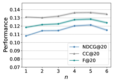
Figure 3: Performance of L$k$P_PS at different $n$.

Figure 3 shows L$k$P_PS performance (Top-5 and Top-20) on Beauty with different numbers of unobserved items (i.e., $n$). We find that all three metrics at different rankings show a similar trend. That is, they smoothly increase at first and then decrease. These results mean that the moderate size of $n$ provides a sufficient set-level ranking comparison for learning $k$-DPP probabilities. However, when redundant comparisons are provided (e.g., $n>5$), it becomes difficult for $k$-DPP to capture effective correlations. As mentioned in Section III-B, we set $k=n$ and the number of targets in the ground set equals to $k$ for L$k$P_NPS and L$k$P_PS to keep the ranking interpretation. External experiments in the cases of $n>k$ on NPS and the number of targets (6 and 7) $>k$ (5) on PS have been performed. However, the worse performance compared to the presented cases suggests the importance of maintaining the ranking interpretation. Experiments in Figure 2 and Figure 3 are conducted on GCN implementation. Similar conclusions are obtained from experiments deployed on MF.

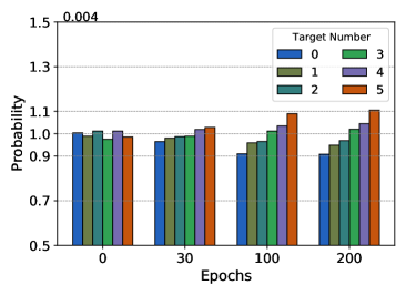
[L$k$P_PS] [L$k$P_NPS]

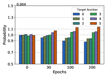
Figure 4: Probability distributions at different epochs on Anime.

To diagrammatically present the ranking interpretation, we use real examples to show the probability ranking of $k$-DPP subsets. We randomly select 100 training instances ($k+n$ ground set where $k=n=5$) in the learning process, and divide all $k$-sized subsets (252) of a ground set into six groups according to the target number in a subset, e.g., the group of $k$-subsets with 1 target comprised of 25 subsets (the subsets filled by 1 observed item and 4 unobserved ones), and target number $=5$ represents the target subset $S_{u}^{+k}$ drawn from a $k$-DPP formulated in Equation 4. The $k$ targets and $n$ random items of training instances contain the same number of categories.

Figure 4 presents probability ranking trends of L$k$P_PS and L$k$P_NPS employing GCN at 0, 30, 100, and 200 training epochs on Beauty. To illustrate the ranking interpretation of $k$-DPP probability learning, probabilities of 252 $k$-sized subsets from each $5+5$ ground set, i.e., $C(5+5,5)$ combinations, are calculated. Before the $k$-DPP learning process starts, randomly distributed subsets (cardinality $k$) are assumed to have the equivalent probability of being selected as a $k$-DPP, i.e., 0.004 (1/252) for each subset. Each bar in a plot denotes the averaged probabilities of subsets that contain the same number of observed items from randomly selected training instances.

We can see that subsets with differing numbers of targets indeed have close normalized $k$-DPP probabilities (i.e., near 0.004) when epoch $=0$. With the learning process proceeding, the discrepancy between $k$-DPP probabilities of subsets with different target numbers obviously grows at first, i.e., subsets with more targets are endowed with higher probabilities, and the trend tends to be stable when epochs reach 200. These illustrate that relevance ranking interpretation behind L$k$P are validated by the $k$-DPP probability examples, as the target subset ranks higher (with greater $k$-DPP probability) than other subsets, and the subset with unobserved items ranks lower than the subsets that contain one or more targets. In addition, considering the exclusion of negative subsets in $k$-DPP (i.e., L$k$P_NPS) facilitates widening the ranking gap between target set and unobserved item set compared to L$k$P_NS, further enhancing performance improvements (as shown in Table II-Table IV). The similar trends can be found on other datasets and MF implementation.

We also conduct a comparison between the averaged $k$-DPP probabilities ($k$=$n$=5) of two types of target subsets on Anime using L$k$P_PS, i.e., monotonous target subsets with limited categories ($<4$ categories) and diversified target subsets with broader categories ($>5$ categories). The observed average probabilities of 0.0041 vs. 0.0040, 0.0045 vs. 0.0042, and 0.0046 vs. 0.0043 for diversified and monotonous target subsets at 0, 100, and 200 epochs respectively, confirm the significant role of diversity ranking interpretation across $(k+n)$ $k$-DPP distributions in our optimization approaches. Because the diverse kernel $\mathbf{K}$ is pre-learned, on average, diverse target sets from half of randomly selected training instances ($k$-DPP distributions) have a relatively higher probability than other monotonous target sets from the $k$-DPP distributions of the remaining half, even before the L$k$P optimization begins.

These results again indicate the importance of $k$-DPP normalization, as only in this case the ranking interpretation is provided. We also perform experiments in the case of removing normalization of $k$-DPP, and then two serious problems occur: (i) the deep learning frameworks (both Pytorch and TensorFlow) cannot handle the complex gradient calculation of the DPP, as the non-normalized determinant values are unstable; (ii) even if we use some techniques, e.g., normalizing diverse kernel or adding activation function to control the values of relevance scores, to avoid the gradient calculation error, the final recommendation results still cannot compare with L$k$P approaches, as the important ranking interpretation for personalized ranking is ignored. These also elucidate why the standard DPP is inapplicable for ranking-based optimization criterion. Within the standard DPP distribution, ranking competition arises among subsets of all sizes, leading to an uninterpretable and ineffective ranking optimization (concrete analysis in Section III-B1). According to our experiments under the same setting as Table II-Table IV, applying standard DPP for the ranking probability formulation (Equation 4) achieves an unacceptable performance that is weaker than BPR (0.1106 vs. 0.1254 at NDCG@20 on ML). This is the reason we omit the results based on standard DPP in this section.

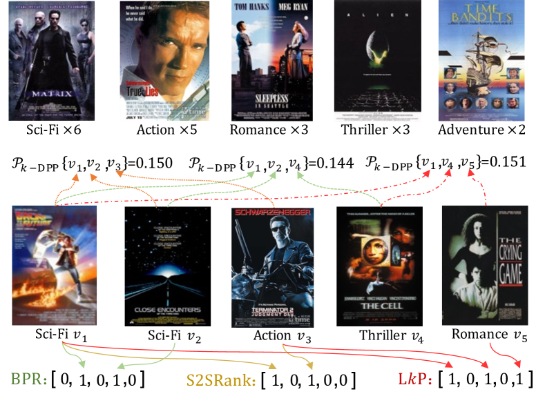
Figure 5: Case study of L$k$P_PS optimization criterion.

In Figure 5, we conduct a case study on $u_{1518}$ of ML-1M using GCN-based L$k$P_PS. For clarity, we categorize each movie reviewed by $u_{1518}$ into a key genre based on its synopsis on Wikipedia. Five genres emerge in the training data, while the test data comprises five movies across four genres. Training movies reveal the user’s inclination towards Sci-Fi (6) and Action (5) movies. Both BPR and S2SRank methods acknowledge this preference by recommending target movies (denoted as 1) in the predicted Top 5 list at positions 2 and 4, and 1 and 3 respectively. Our L$k$P method, while recognizing the user’s apparent preferences, also considers diversity by suggesting a hidden target romance movie. This highlights L$k$P’s ability to cater to relevance and diversity. We also analyze $k$-DPP probabilities for 3-sized subsets over movies for testing and observe: (i) The diversified item subset $\{v_{1},v_{4},v_{5}\}$ has a higher probability than monotonous ones, affirming our consideration on diversity comparison; (ii) Despite similar category scopes, the subset $\{v_{1},v_{2},v_{3}\}$ possesses a higher probability than $\{v_{1},v_{2},v_{4}\}$, which suggests that a stronger dependency between $v_{3}$ and $\{v_{1},v_{2}\}$ leads to a higher predictive value for $v_{3}$, further emphasizing the capability of concrete set-level ranking to capture intricate relationships.

V Conclusion

In this work, we propose a new optimization criterion L$k$P based on $k$-DPP set probability comparison for personalized ranking focusing on implicit feedback, enlightening a new perspective (set-level probability comparison) in the formulation of ranking optimization. Based on this, two ranking optimization approaches L$k$P_PS and L$k$P_NPS are designed that take into account different ranking considerations. As such, multiple observed items and unobserved items are directly regarded as subsets with fixed cardinality $k$, and are compared through the ranking interpretation based on the tailored $k$-DPP distribution, notably with probabilistic normalization that respects the cardinality constraint. Three levels of evaluation and comparison in the experiments comprehensively demonstrate the superiority of our approaches, and the ranking interpretation is validated through real-world examples. Notably, plugging our optimization criterion into strong baselines provides a ready source of improved performance. Experimental results help us to analyze the different advantages of two L$k$P approaches and provide insight into making selection between them in different circumstances. L$k$P_PS and L$k$P_NPS also have potential in ranking related tasks, such as Web search [52, 53] and spam detection [54, 55, 56], which will be explored in the future.

References

- [1] S. Rendle, C. Freudenthaler, Z. Gantner, and L. Schmidt-Thieme, “Bpr: Bayesian personalized ranking from implicit feedback,” arXiv preprint arXiv:1205.2618, 2012.
- [2] X. He, L. Liao, H. Zhang, L. Nie, X. Hu, and T.-S. Chua, “Neural collaborative filtering,” in Proceedings of the 26th international conference on world wide web, 2017, pp. 173–182.
- [3] Z. Cao, T. Qin, T.-Y. Liu, M.-F. Tsai, and H. Li, “Learning to rank: from pairwise approach to listwise approach,” in Proceedings of the 24th international conference on Machine learning, 2007, pp. 129–136.
- [4] F. Xia, T.-Y. Liu, J. Wang, W. Zhang, and H. Li, “Listwise approach to learning to rank: theory and algorithm,” in Proceedings of the 25th international conference on Machine learning, 2008, pp. 1192–1199.
- [5] C. Wang, H. Zhu, C. Zhu, C. Qin, and H. Xiong, “Setrank: A setwise bayesian approach for collaborative ranking from implicit feedback,” in Proceedings of the aaai conference on artificial intelligence, vol. 34, no. 04, 2020, pp. 6127–6136.
- [6] L. Chen, L. Wu, K. Zhang, R. Hong, and M. Wang, “Set2setrank: collaborative set to set ranking for implicit feedback based recommendation,” in Proceedings of the 44th International ACM SIGIR Conference on Research and Development in Information Retrieval, 2021, pp. 585–594.
- [7] Q. Wu, Y. Liu, C. Miao, B. Zhao, Y. Zhao, and L. Guan, “Pd-gan: Adversarial learning for personalized diversity-promoting recommendation.” in IJCAI, vol. 19, 2019, pp. 3870–3876.
- [8] R. Boim, T. Milo, and S. Novgorodov, “Direc: Diversified recommendations for semantic-less collaborative filtering,” in 2011 IEEE 27th International Conference on Data Engineering (ICDE). IEEE, 2011, pp. 1312–1315.
- [9] X. Su and T. M. Khoshgoftaar, “A survey of collaborative filtering techniques,” Advances in artificial intelligence, vol. 2009, 2009.
- [10] S. Wu, W. Ren, C. Yu, G. Chen, D. Zhang, and J. Zhu, “Personal recommendation using deep recurrent neural networks in netease,” in 2016 IEEE 32nd international conference on data engineering (ICDE). IEEE, 2016, pp. 1218–1229.
- [11] A. Mnih and R. R. Salakhutdinov, “Probabilistic matrix factorization,” Advances in neural information processing systems, vol. 20, 2007.
- [12] Y. Koren, R. Bell, and C. Volinsky, “Matrix factorization techniques for recommender systems,” Computer, vol. 42, no. 8, pp. 30–37, 2009.
- [13] Y. Koren, “Factorization meets the neighborhood: a multifaceted collaborative filtering model,” in Proceedings of the 14th ACM SIGKDD international conference on Knowledge discovery and data mining, 2008, pp. 426–434.
- [14] Z. Li, X. Shen, Y. Jiao, X. Pan, P. Zou, X. Meng, C. Yao, and J. Bu, “Hierarchical bipartite graph neural networks: Towards large-scale e-commerce applications,” in 2020 IEEE 36th International Conference on Data Engineering (ICDE). IEEE, 2020, pp. 1677–1688.
- [15] H. Wang, N. Wang, and D.-Y. Yeung, “Collaborative deep learning for recommender systems,” in Proceedings of the 21th ACM SIGKDD international conference on knowledge discovery and data mining, 2015, pp. 1235–1244.
- [16] L. Chen, L. Wu, R. Hong, K. Zhang, and M. Wang, “Revisiting graph based collaborative filtering: A linear residual graph convolutional network approach,” in Proceedings of the AAAI conference on artificial intelligence, vol. 34, no. 01, 2020, pp. 27–34.
- [17] Y. Tay, L. Anh Tuan, and S. C. Hui, “Latent relational metric learning via memory-based attention for collaborative ranking,” in Proceedings of the 2018 world wide web conference, 2018, pp. 729–739.
- [18] R. He, W.-C. Kang, and J. McAuley, “Translation-based recommendation,” in Proceedings of the eleventh ACM conference on recommender systems, 2017, pp. 161–169.
- [19] Y. Chen, Y. Yang, Y. Wang, J. Bai, X. Song, and I. King, “Attentive knowledge-aware graph convolutional networks with collaborative guidance for personalized recommendation,” in 2022 IEEE 38th International Conference on Data Engineering (ICDE). IEEE, 2022, pp. 299–311.
- [20] J. Zhao, P. Zhao, L. Zhao, Y. Liu, V. S. Sheng, and X. Zhou, “Variational self-attention network for sequential recommendation,” in 2021 IEEE 37th International Conference on Data Engineering (ICDE). IEEE, 2021, pp. 1559–1570.
- [21] Q. Wan, X. He, X. Wang, J. Wu, W. Guo, and R. Tang, “Cross pairwise ranking for unbiased item recommendation,” in Proceedings of the ACM Web Conference 2022, 2022, pp. 2370–2378.
- [22] C. Gao, X. He, D. Gan, X. Chen, F. Feng, Y. Li, T.-S. Chua, and D. Jin, “Neural multi-task recommendation from multi-behavior data,” in 2019 IEEE 35th international conference on data engineering (ICDE). IEEE, 2019, pp. 1554–1557.
- [23] Y. Shi, M. Larson, and A. Hanjalic, “List-wise learning to rank with matrix factorization for collaborative filtering,” in Proceedings of the fourth ACM conference on Recommender systems, 2010, pp. 269–272.
- [24] R. Yu, Q. Liu, Y. Ye, M. Cheng, E. Chen, and J. Ma, “Collaborative list-and-pairwise filtering from implicit feedback,” IEEE Transactions on Knowledge and Data Engineering, 2020.
- [25] L. Chen, G. Zhang, and E. Zhou, “Fast greedy map inference for determinantal point process to improve recommendation diversity,” Advances in Neural Information Processing Systems, vol. 31, 2018.
- [26] Y. Liu, Y. Xiao, Q. Wu, C. Miao, J. Zhang, B. Zhao, and H. Tang, “Diversified interactive recommendation with implicit feedback,” in Proceedings of the AAAI Conference on Artificial Intelligence, vol. 34, no. 04, 2020, pp. 4932–4939.
- [27] L. Gan, D. Nurbakova, L. Laporte, and S. Calabretto, “Enhancing recommendation diversity using determinantal point processes on knowledge graphs,” in Proceedings of the 43rd International ACM SIGIR Conference on Research and Development in Information Retrieval, 2020, pp. 2001–2004.
- [28] M. Gartrell, U. Paquet, and N. Koenigstein, “Low-rank factorization of determinantal point processes,” in Thirty-First AAAI Conference on Artificial Intelligence, 2017.
- [29] I. Goodfellow, J. Pouget-Abadie, M. Mirza, B. Xu, D. Warde-Farley, S. Ozair, A. Courville, and Y. Bengio, “Generative adversarial networks,” Communications of the ACM, vol. 63, no. 11, pp. 139–144, 2020.
- [30] R. Warlop, J. Mary, and M. Gartrell, “Tensorized determinantal point processes for recommendation,” in Proceedings of the 25th ACM SIGKDD International Conference on Knowledge Discovery & Data Mining, 2019, pp. 1605–1615.
- [31] X. Wang, X. He, M. Wang, F. Feng, and T.-S. Chua, “Neural graph collaborative filtering,” in Proceedings of the 42nd international ACM SIGIR conference on Research and development in Information Retrieval, 2019, pp. 165–174.
- [32] Y. Liang and T. Qian, “Recommending accurate and diverse items using bilateral branch network,” arXiv preprint arXiv:2101.00781, 2021.
- [33] A. Kulesza, B. Taskar et al., “Determinantal point processes for machine learning,” Foundations and Trends® in Machine Learning, vol. 5, no. 2–3, pp. 123–286, 2012.
- [34] A. Kulesza and B. Taskar, “k-dpps: Fixed-size determinantal point processes,” in ICML, 2011.
- [35] Y. Liu, C. Walder, and L. Xie, “Determinantal point process likelihoods for sequential recommendation,” arXiv preprint arXiv:2204.11562, 2022.
- [36] R. L. Santos, C. Macdonald, and I. Ounis, “Exploiting query reformulations for web search result diversification,” in Proceedings of the 19th international conference on World wide web, 2010, pp. 881–890.
- [37] S. A. Puthiya Parambath, N. Usunier, and Y. Grandvalet, “A coverage-based approach to recommendation diversity on similarity graph,” in Proceedings of the 10th ACM Conference on Recommender Systems, 2016, pp. 15–22.
- [38] X. He, K. Deng, X. Wang, Y. Li, Y. Zhang, and M. Wang, “Lightgcn: Simplifying and powering graph convolution network for recommendation,” in Proceedings of the 43rd International ACM SIGIR conference on research and development in Information Retrieval, 2020, pp. 639–648.
- [39] I. M. Gelfand, Lectures on linear algebra. Courier Corporation, 1989.
- [40] M. L. Fisher, G. L. Nemhauser, and L. A. Wolsey, An analysis of approximations for maximizing submodular set functions—II. Springer, 1978.
- [41] R. He and J. McAuley, “Ups and downs: Modeling the visual evolution of fashion trends with one-class collaborative filtering,” in proceedings of the 25th international conference on world wide web, 2016, pp. 507–517.
- [42] R. H. Affandi, E. Fox, R. Adams, and B. Taskar, “Learning the parameters of determinantal point process kernels,” in International Conference on Machine Learning. PMLR, 2014, pp. 1224–1232.
- [43] C. Yu, L. V. Lakshmanan, and S. Amer-Yahia, “Recommendation diversification using explanations,” in 2009 IEEE 25th International Conference on Data Engineering (ICDE). IEEE, 2009, pp. 1299–1302.
- [44] Z. Chen, T. Xiao, and K. Kuang, “Ba-gnn: On learning bias-aware graph neural network,” in 2022 IEEE 38th International Conference on Data Engineering (ICDE). IEEE, 2022, pp. 3012–3024.
- [45] R. v. d. Berg, T. N. Kipf, and M. Welling, “Graph convolutional matrix completion,” arXiv preprint arXiv:1706.02263, 2017.
- [46] X. Wang, X. He, Y. Cao, M. Liu, and T.-S. Chua, “Kgat: Knowledge graph attention network for recommendation,” in Proceedings of the 25th ACM SIGKDD international conference on knowledge discovery & data mining, 2019, pp. 950–958.
- [47] J. Zhang, C. Gao, D. Jin, and Y. Li, “Group-buying recommendation for social e-commerce,” in 2021 IEEE 37th International Conference on Data Engineering (ICDE). IEEE, 2021, pp. 1536–1547.
- [48] H. Yin, Q. Wang, K. Zheng, Z. Li, J. Yang, and X. Zhou, “Social influence-based group representation learning for group recommendation,” in 2019 IEEE 35th International Conference on Data Engineering (ICDE). IEEE, 2019, pp. 566–577.
- [49] Y. Zheng, C. Gao, X. He, Y. Li, and D. Jin, “Price-aware recommendation with graph convolutional networks,” in 2020 IEEE 36th International Conference on Data Engineering (ICDE). IEEE, 2020, pp. 133–144.
- [50] P. Cheng, S. Wang, J. Ma, J. Sun, and H. Xiong, “Learning to recommend accurate and diverse items,” in Proceedings of the 26th international conference on World Wide Web, 2017, pp. 183–192.
- [51] M. Zhang and N. Hurley, “Avoiding monotony: improving the diversity of recommendation lists,” in Proceedings of the 2008 ACM conference on Recommender systems, 2008, pp. 123–130.
- [52] K. W.-T. Leung, D. L. Lee, and W.-C. Lee, “Personalized web search with location preferences,” in 2010 IEEE 26th International Conference on Data Engineering (ICDE 2010). IEEE, 2010, pp. 701–712.
- [53] G. Kasneci, F. M. Suchanek, G. Ifrim, M. Ramanath, and G. Weikum, “Naga: Searching and ranking knowledge,” in 2008 IEEE 24th International Conference on Data Engineering. IEEE, 2008, pp. 953–962.
- [54] P.-A. Chirita, J. Diederich, and W. Nejdl, “Mailrank: using ranking for spam detection,” in Proceedings of the 14th ACM international conference on Information and knowledge management, 2005, pp. 373–380.
- [55] M. Saini, S. Verma, and A. Sharan, “Multi-view ensemble learning using rough set based feature ranking for opinion spam detection,” in Advances in computer communication and computational sciences. Springer, 2019, pp. 3–12.
- [56] Y. Liu, “Recommending inferior results: A general and feature-free model for spam detection,” in Proceedings of the 29th ACM International Conference on Information & Knowledge Management, 2020, pp. 955–974.