Towards Exact Computation of Inductive Bias

Abstract

Much research in machine learning involves finding appropriate inductive biases (e.g. convolutional neural networks, momentum-based optimizers, transformers) to promote generalization on tasks. However, quantification of the amount of inductive bias associated with these architectures and hyperparameters has been limited. We propose a novel method for efficiently computing the inductive bias required for generalization on a task with a fixed training data budget; formally, this corresponds to the amount of information required to specify well-generalizing models within a specific hypothesis space of models. Our approach involves modeling the loss distribution of random hypotheses drawn from a hypothesis space to estimate the required inductive bias for a task relative to these hypotheses. Unlike prior work, our method provides a direct estimate of inductive bias without using bounds and is applicable to diverse hypothesis spaces. Moreover, we derive approximation error bounds for our estimation approach in terms of the number of sampled hypotheses. Consistent with prior results, our empirical results demonstrate that higher dimensional tasks require greater inductive bias. We show that relative to other expressive model classes, neural networks as a model class encode large amounts of inductive bias. Furthermore, our measure quantifies the relative difference in inductive bias between different neural network architectures. Our proposed inductive bias metric provides an information-theoretic interpretation of the benefits of specific model architectures for certain tasks and provides a quantitative guide to developing tasks requiring greater inductive bias, thereby encouraging the development of more powerful inductive biases.

1 Introduction

Generalization is a fundamental challenge in machine learning, as models must be able to perform well on unseen data after being trained on a limited set of examples. To achieve this, researchers have extensively studied the role of inductive biases, which are prior assumptions or restrictions embedded within learning algorithms, in promoting generalization. These biases can take various forms, such as architectural choices (e.g., convolutional neural networks, momentum-based optimizers, transformers) or hyperparameter settings, and they shape the space of hypotheses that the model can consider.

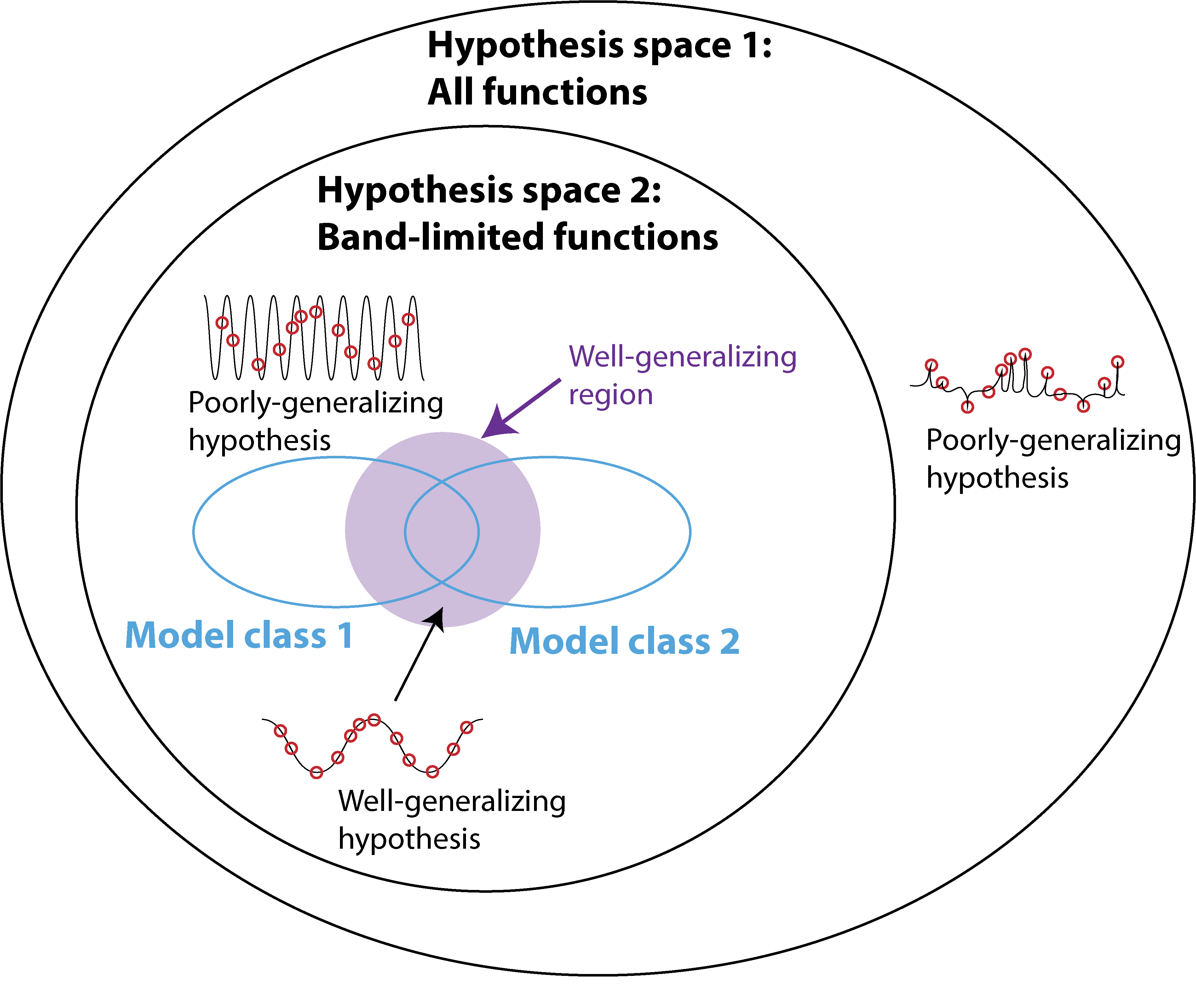
Despite the importance of inductive biases, quantifying the amount of inductive bias associated with different architectural and hyperparameter choices has remained challenging. Inductive bias can be formulated as the amount of information required to specify well-generalizing models within a hypothesis space of models Chollet (2019); Boopathy et al. (2023). Like a model class, a hypothesis space is a set of models; however, while a model class corresponds to a specific set of inductive biases (e.g. a particular architecture), a hypothesis space is a set in which all relevant model classes are contained. We make a distinction between hypothesis spaces and model classes to illustrate that hypothesis spaces are typically much broader than model classes and set the context under which inductive biases can be evaluated; for instance, a model class may be a particular convolutional neural network architecture, while the hypothesis space may consist of all functions expressible by any finite-sized neural network.

Previous attempts at measuring inductive bias have often provided only upper bounds or have been limited to specific model classes. This limitation hinders a comprehensive understanding of how different biases contribute to generalization and impedes the systematic development of more effective biases.

In this paper, we propose a novel and efficient method for computing the inductive bias required for generalization on a task under fixed training data budget. Unlike prior work, our approach provides a direct estimate of inductive bias without relying on bounds. Moreover, it is applicable to diverse hypothesis spaces, allowing the computation of inductive bias within the context of particular model classes such as neural networks. We believe more precise and flexible computation of inductive bias is practically valuable:

First, by quantifying the amount of inductive bias associated with different architectural choices, researchers can gain profound insights into how specific design decisions affect the model’s ability to generalize. This understanding helps identify which architectural features contribute most significantly to improved performance and informs the development of more tailored and task-specific models. Armed with a quantitative measure of inductive bias, practitioners can make more informed decisions about which architectural choices to prioritize when building and optimizing machine learning models. This, in turn, can lead to more efficient model development processes and improved real-world applications.

Second, our inductive bias measure serves as a practical guide for designing tasks that demand higher levels of inductive bias. By precisely estimating the amount of inductive bias needed for a given task, researchers can intentionally craft benchmarks that challenge the boundaries of generalizability of current models. This approach encourages the development of more powerful model architectures and learning algorithms, fostering innovation in the field.

We summarize our contributions as follows:

• We propose a definition of inductive bias with an explicit dependence on the hypothesis space within which models are defined.

• We develop an efficient sampling-based algorithm to compute the inductive bias required to generalize on a task. Unlike prior work, the method can be applied to parametric and non-parametric hypothesis spaces.

• We derive an upper bound on the approximation error of inductive bias estimate; the approximation error scales inversely with the number of sampled hypotheses.

• We empirically apply our inductive bias metric to a range of domains including supervised image classification, reinforcement learning (RL) and few-shot meta-learning. Consistent with prior work, we find that tasks with higher dimensional inputs require more inductive bias.

• We empirically find that neural networks encode massive amounts of inductive bias relative to other expressive model classes. Furthermore, we quantify the difference in inductive bias provided by different neural network architectures within a neural network hypothesis space.

2 Related Work

Generalization vs. Sample Complexity

Traditionally, the generalizability of machine learning models has been analyzed in terms of sample complexity, which is the amount of training data required to generalize on a task Cortes et al. (1994); Murata et al. (1992); Amari (1993); Hestness et al. (2017). Measures such as Rademacher complexity Koltchinskii and Panchenko (2000) and VC dimension Blumer et al. (1989) quantify the capacity of a model class and provide upper bounds on sample complexity, with less expressive model classes requiring fewer samples. More recently, data-dependent generalization bounds have been proposed, yielding tighter bounds based on dataset properties Negrea et al. (2019); Raginsky et al. (2016); Kawaguchi et al. (2022); Lei et al. (2015); Jiang et al. (2021). Additionally, scaling laws for neural networks have modeled learning as kernel regression, revealing that sample complexity scales exponentially with the intrinsic dimensionality of data Bahri et al. (2021); Hutter (2021); Sharma and Kaplan (2022). In our work, instead of focusing on the importance of training data in generalization, we focus on the role of inductive biases.

Generalization vs. Inductive Bias Complexity

The importance of inductive biases in promoting generalization has been widely recognized, starting with the No Free Lunch theorem Wolpert (1996) which states that no learning algorithm can perform well on all possible tasks: learning algorithms require inductive biases tailored to specific sets of tasks. Subsequent studies have further emphasized the role of inductive biases in learning Hernández-Orallo (2016); Haussler (1988); Du et al. (2018); Li et al. (2021), showing that specific abilities, biases, and model architectures provide prior knowledge that facilitates generalization. Despite the central role of inductive biases, work on quantifying them has been limited. Chollet (2019) proposes measuring the generalization difficulty of a task as the amount of inductive bias required for a learning system to perform the task in addition to any training data provided. Boopathy et al. (2023) provides an upper bound on the inductive bias complexity of a task (i.e. how much inductive bias is required to generalize on a task) based on task properties. In particular, it finds that higher-dimensional tasks (i.e. tasks with inputs of higher intrinsic dimensionality) require exponentially greater inductive bias, mirroring results for sample complexity. In this work, we aim to more precisely and directly estimate the required inductive bias of a task without the use of bounds. Moreover, unlike prior work, our approach can compute inductive bias complexity within general hypothesis spaces: it allows for context-specific computation of inductive bias. For instance, we may compute the inductive bias required to generalize on ImageNet Deng et al. (2009) classification under 1) a hypothesis space of general neural networks vs. 2) a hypothesis space consisting only of convolutionally-structured neural networks, under which less inductive bias is required.

Figure 1: An illustration of example hypothesis spaces, model classes, and specific models for a particular learning problem. Red circles indicate training points and black curves indicate hypotheses. A hypothesis space sets the broad set of models we wish to consider. In this illustration, we consider the hypothesis space of all functions and a smaller hypothesis space of band-limited functions (i.e. functions with limited maximum frequency). A model class is a set of models associated with a particular set of inductive biases. We measure the required amount of inductive bias to solve a task based on the size of the well-generalizing region within the context of a particular hypothesis space.

3 Quantifying Inductive Bias

In this section, we present our method for quantifying the inductive bias of a model class. Inductive bias, in simple terms, represents the inherent assumptions or characteristics of a model class that influence its ability to generalize to new, unseen data. We first provide a formal quantitative definition of the amount of inductive bias of a model class. We then propose our method of approximating this amount of inductive bias and prove a bound on its error.

Figure 2: Illustration of how the required inductive bias for a task can be computed from the hypothesis space and the region of well-generalizing hypotheses. Black boxes indicate hypothesis spaces; $p_{h}$ is a uniform distribution over each box. Purple indicates regions of well-generalizing hypotheses. Inductive bias is the negative log of the fraction of hypothesis space that generalizes well: $I=-\log\frac{Hypothesis\,space\cap Well-generalizing\,hypotheses}{Hypothesis\,space}$. It depends on both the size of the hypothesis space as well as how much the hypothesis space overlaps with well-generalizing hypotheses. Different hypothesis spaces may yield different inductive bias estimates even on the same task (i.e. the same set of well-generalizing hypotheses).

3.1 Definition of Inductive Bias

Intuitively, inductive biases are guiding principles that help models make sense of data. For instance, when we look at an image of a cat, we rely on our inductive bias to recognize it as a cat, based on features like whiskers, fur, and ears. In machine learning, model classes (e.g. convolutional neural networks) have inductive biases (e.g. invariance to translation of inputs) which are essential for sample-efficient learning.

Boopathy et al. (2023) proposes quantifying the amount of inductive bias required to generalize on a task based on the probability that a model that fits a training set also generalizes to a test set. Importantly, this definition assumes that there exists a hypothesis space of models. Formally, the hypothesis space contains all possible models to solve a specific problem (i.e. the universe of potential solutions). A model is a specific hypothesis from this space. A model class is a subset of this space, chosen by a model designer, typically including well-generalizing models. Inductive bias, then, quantifies the amount of information needed to specify a well-generalizing model class within the hypothesis space. In simpler terms, it measures how much ”guidance” a model needs from the model designer to perform well on a task. See Figure 1 for an illustration of these concepts.

Note that the size of the hypothesis space can strongly affect the magnitude of the inductive bias, but in Boopathy et al. (2023) the dependence on the hypothesis is implicit. Here we formally define inductive bias in a similar manner to Boopathy et al. (2023) but provide a way to explicitly include the distribution of models in the hypothesis space (e.g. neural networks versus Gaussian RBF models; or more finely, different neural network architectures). Our approach applies across a variety of domains ranging from supervised classification to RL as we will empirically show. Our formal definition follows:

Definition 1.

Let $\mathcal{H}$ be a set of hypotheses, and let hypothesis distribution $p_{h}$ define a probability distribution over these hypotheses. Suppose there exists a loss function $L$ that maps a hypothesis $h\in\mathcal{H}$ and a task input $x\in\mathcal{X}$ to a scalar: $L:\mathcal{H}\times\mathcal{X}\to\mathbb{R}$. Finally, suppose there exists a test distribution $p_{x}$ over the task inputs. With respect to distribution $p_{h}$, the amount of inductive bias required to achieve test set error rate $\varepsilon$ on a task is:

$$I(\varepsilon,p_{h},p_{x},L)=-\log\int\mathbf{1}(\mathbb{E}_{x\sim p_{x}}[L(h,x)]\leq\varepsilon)p_{h}(h)dh$$ (1)

where $\mathbf{1}$ denotes the indicator function.

Note that this is simply negative log of the probability that a hypothesis sampled from $p_{h}$ achieves an error rate $\leq\varepsilon$ on a test set. $p_{h}$ may be any distribution over the hypothesis space; Boopathy et al. (2023) sets $p_{h}$ as a uniform distribution of models achieving a training set error $\leq\epsilon$. In practice, we may be interested in the case when $p_{h}$ is a distribution of models produced by an optimization process on a training set. This allows us to quantify the additional inductive bias required to generalize on top of any information provided by the training data. Critically, as Figure 2 illustrates, the specific choice of $p_{h}$ has a significant impact on the inductive bias. Intuitively, if the hypothesis distribution is more aligned with a task, fewer inductive biases are required to generalize.

Estimating this inductive bias by directly sampling hypotheses from a hypotheses space is computationally infeasible for large hypothesis spaces since the vast majority of hypotheses may not generalize well. Thus, we propose a two-phase approach to compute the inductive bias: first, we sample from the hypothesis space and compute an empirical distribution of test set error values $\mathbb{E}_{x\sim p_{x}}[L(h,x)]$. Few (or none) of these hypotheses may generalize at the desired error rate. Thus, we use the samples to model the test error distribution to estimate the probability of achieving test error $\leq\varepsilon$.

We also note that inductive bias in Equation 1 is a function of the desired error rate $\varepsilon$; it is not a function of a specific model or model class, although it is a function of the hypothesis distribution $p_{h}$. However, we may use this definition to compute the inductive bias provided by a specific model under a specific hypothesis space by computing the amount of inductive bias required to generalize at the level of the model (i.e. by plugging in the model’s test set error rate $\varepsilon$ into Equation 1). This allows us to understand how the inductive bias of a model is affected by the properties of the broader hypothesis space, and how it contributes to the model’s generalization.

3.2 Efficiently Sampling from the Hypothesis Space

Here, we aim to efficiently sample hypotheses from $p_{h}$, where we assume $p_{h}$ includes only hypotheses fitted to a training set. We use two approaches: directly optimizing the parameters of a hypothesis (i.e. training a model on the training data), or a kernel-based sampling approach.

Direct Optimization by Gradient Descent

For hypothesis spaces with a known, finite-dimensional parameterization, it may be reasonable to set $p_{h}$ as a distribution of hypotheses produced by performing gradient descent on loss function $L$ evaluated on a training set of data $x$. For instance, $p_{h}$ may correspond to a distribution of neural networks after training from random initialization by gradient descent on a training set. Given $P$ parameters per hypothesis, performing each step of gradient descent takes $O(P)$ time, yielding $O(PT)$ time for $T$ optimization steps. Thus, producing $S$ samples requires $O(SPT)$ time.

Kernel-based Sampling

If the hypothesis space is very high-dimensional, direct optimization may be computationally challenge, and for infinite-dimensional models, representing the parameters themselves may be infeasible. Instead, we formulate the problem of sampling from a hypothesis space as sampling from a Gaussian process, for which efficient algorithms have been extensively studied. We use an algorithm resembling the approach of Lin et al. (2023). The key principle behind our algorithm is to reparameterize the distribution of hypothesis output values on a test set in terms of a unit Gaussian. This allows us to easily and efficiently draw samples from this distribution in linear time (in terms of training set size).

We assume hypotheses $h$ are linearly parameterized with parameters $\theta\in\mathbb{R}^{P}$ as:

$$h(x)=\phi(x)\theta$$ (2)

where $\phi(x)\in\mathbb{R}^{k\times P}$ is a dimensional feature matrix and $k$ is the dimensionality of $h(x)$. This type of assumption is standard for kernel methods including neural networks in the Gaussian process or Neural Tangent Kernel limits. Here, we set $p_{h}$ to include only the set of hypotheses that interpolate the training data. Given a set of $N$ training points $X$, their corresponding features $\phi(X)\in\mathbb{R}^{Nk\times P}$ and target model outputs $Y\in\mathbb{R}^{Nk}$, where $k$ represents output dimensionality, observe that if a hypothesis interpolates the training data, its parameters must satisfy:

$$Y=\phi(X)\theta$$ (3)

We may decompose $\theta$ into two terms:

$$\theta=\phi(X)^{\dagger}Y+\beta$$ (4)

where $\beta\in\mathbb{R}^{P}$ satisfies $\phi(X)\beta=0$. The first term ensures the hypothesis fits the training data while the second term allows for variation between hypotheses. Finally, we set $\beta$ as a Gaussian with mean $0$ and covariance $I-\phi(X)^{\dagger}\phi(X)$, where $\dagger$ represents pseudoinverse. This corresponds to setting the distribution of parameters $\theta$ as:

$$p_{\theta}(\theta)=\mathcal{N}(\phi(X)^{\dagger}Y,I-\phi(X)^{\dagger}\phi(X))$$ (5)

This corresponds to a Gaussian process conditioned on the training points.

We aim to sample the value of $h$ on a test set $\bar{X}$ consisting of $n$ points. These values $h(\bar{X})$ may be computed as:

$$h(\bar{X})=K(\bar{X},X)\alpha^{*}+\sqrt{K(\bar{X},\bar{X})-K(\bar{X},X)A^{*}}z$$ (6)

where $\alpha^{*}$ and $A^{*}$ are found as:

$$\alpha^{*}=\operatorname*{arg\,min}_{\alpha}||Y-K(X,X)\alpha||_{2}^{2}$$ (7)

$$A^{*}=\operatorname*{arg\,min}_{A}||K(X,\bar{X})-K(X,X)A||_{F}^{2}$$ (8)

and $z$ is drawn from a unit Gaussian $\mathcal{N}(0,I)$. We find approximate solutions to these optimization problems by stochastic gradient descent. Pseudocode is provided in Algorithm 1, with additional details included in the Appendix. Producing $S$ samples requires a total of $O(nNk^{2}T+n^{3}k^{3}+n^{2}Nk^{3}+n^{2}k^{2}S)$ time where $T$ is the number of optimization steps. In practice, the $nNk^{2}T$ term dominates due to the large size of $T$: this implies that we may increase the number of drawn samples $S$ with no asymptotic impact on the runtime.

Algorithm 1 Kernel-based Sampling

0:  $X,Y,\bar{X},n,k,T,S,\eta$

1:  Initialize $\alpha$ and $A$ with zeros

2:  for $t=1$ to $T$ do

3:     Randomly sample a mini-batch of training examples $(x,y)\in(X,Y)$

4:     $g_{\alpha}=2K(X,x)(K(x,X)\alpha-y)$

5:     $g_{A}=2K(X,x)(K(x,\bar{X})A-K(x,\bar{X}))$

6:     $\alpha\leftarrow\alpha-\eta g_{\alpha}$

7:     $A\leftarrow A-\eta g_{A}$

8:  end for

9:  $m=K(\bar{X},X)\alpha$

10:  $\sqrt{C}=\sqrt{K(\bar{X},\bar{X})-K(\bar{X},X)A}$

11:  Initialize an empty list $\mathtt{samples}$

12:  for $s=1$ to $S$ do

13:     Sample $z\sim\mathcal{N}(0,I)$

14:     $h(\bar{X})=m+\sqrt{C}z$

15:     Append $h(\bar{x}_{s})$ to $\mathtt{samples}$

16:  end for

17:  Return $\mathtt{samples}$

3.3 Modeling the Test Error Distribution

Once we generate samples from the hypothesis space, we next aim to model the distribution of test set losses of sampled functions from the hypothesis space; this allows us to compute inductive bias.

To understand the shape of the test loss distribution, we return to the assumptions in the kernel-based sampling of the hypothesis space. We assume that the regression targets $Y,\bar{Y}$ on the training and test sets respectively are constructed as $Y=\phi(X)\theta^{*},\bar{Y}=\phi(\bar{X})\theta^{*}$ for unknown parameters $\theta^{*}$.

The squared error between the prediction $h(\bar{X})$ and true value $\bar{Y}$ may be written as:

$$||h(\bar{X})-\bar{Y}||_{2}^{2}\\ =||\phi(\bar{X})\phi(X)^{\dagger}\phi(X)\theta^{*}+\phi(\bar{X})\beta-\phi(\bar{X})\theta^{*}||_{2}^{2}$$ (9)

We may write $\beta$ as $\beta=(I-\phi(X)^{\dagger}\phi(X))\xi$ where $\xi\in\mathbb{R}^{P}$ is distributed as a unit Gaussian. Then, the squared prediction error may be written as:

$$||h(\bar{X})-\bar{Y}||_{2}^{2}=||\phi(\bar{X})(I-\phi(X)^{\dagger}\phi(X))(\xi-\theta^{*})||_{2}^{2}$$ (10)

Observe that this is a quadratic form of a Gaussian random variable $\xi-\theta^{*}$; thus, $||h(\bar{X})-\bar{Y}||_{2}^{2}$ follows a generalized Chi-squared distribution.

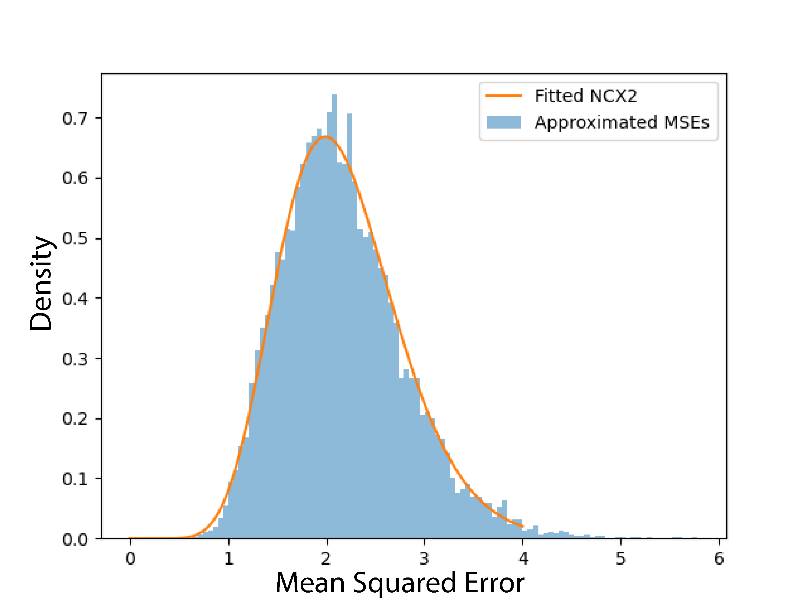
In practice, to minimize the number of fit parameters when modeling the empirical error distribution, we fit the test loss using a scaled non-central Chi-squared (which is a special case of a generalized Chi-squared distribution); this has three fit parameters. These parameters are fit with maximum likelihood estimation. Figure 3 illustrates that this distribution is able to closely fit test errors of random hypotheses on a real dataset.

Figure 3: Fitting a scaled non-central Chi-squared distribution to an empirical distribution of mean squared errors of models drawn from a kernel-based Gaussian RBF hypothesis space on a restricted version of MNIST. Observe that the distribution closely models the empirical distribution.

Since we model the test error distribution as a Chi-squared distribution, we need to approximate the negative log of the cumulative distribution function (CDF) given its parameters. Given a Chi-squared distribution with $k$ degrees of freedom and non-centrality parameter $\lambda$, we use the following approximation by Sankaran Sankaran (1959) for the CDF:

$$P(z;k,\lambda)\\ \approx\Phi\left[\frac{\left(\frac{z}{k+\lambda}\right)^{h}-(1+hp(h-1-0.5(2-h)mp))}{h\sqrt{2p}(1+0.5mp)}\right],$$ (11)

where $\Phi$ is the CDF of a standard normal random variable and

$$h=1-\frac{2}{3}\frac{(k+\lambda)(k+3\lambda)}{(k+2\lambda)^{2}},\qquad p=\frac{k+2\lambda}{(k+\lambda)^{2}},\\ m=(h-1)(1-3h).$$ (12)

This approximation is more accurate when $k$ is large, which corresponds to higher-dimensional parameter spaces; for lower dimensional spaces, it may be more appropriate to directly compute the CDF of the Chi-squared distribution. Finally, we use a Chernoff bound-based approximation $\Phi(-z)\approx e^{\frac{-z^{2}}{2}}$ to finish the calculation. Specifically, since the inductive bias is given as the negative log probability of generalizing up to error rate $\varepsilon$ (see Equation 1), we simply compute the negative log of the approximated CDF after plugging in the desired $\varepsilon$ for $z$. The appendix provides further details on how the test error distribution is modeled.

3.4 Bounding the Approximation Error

Next, we derive a bound on the approximation error of our estimate of required inductive bias. At a high level, the bound proceeds as follows: we first bound how closely our samples from the hypothesis distribution match the true distribution $p_{h}$, and then bound the error in our modeling of the test error distribution to arrive at a final bound on the amount of inductive bias.

Theorem 2.

Suppose we are provided a hypothesis distribution $p_{h}$, input distribution $p_{x}$, loss function $L$ and desired error rate $\varepsilon$. Suppose we estimate $I(\varepsilon,p_{h},p_{x},L)$ by first sampling $n$ hypotheses ($h^{1},h^{2},...h^{n}$) iid from $q_{h}$ which is close to $p_{h}$ in the sense that

$$|\log p_{h}(h)-\log q_{h}(h)|\leq\xi_{h}$$ (13)

for all $h$. We then compute the test losses of each hypothesis $\mathbb{E}_{x\sim p_{x}}[L(h^{1},x)],\mathbb{E}_{x\sim p_{x}}[L(h^{2},x)],...\mathbb{E}_{x\sim p_{x}}[L(h^{n},x)]$. Next, we model the distribution of test losses with a distribution $f(l;\alpha)$ where $\alpha$ represents a finite number of parameters. We assume $f$ has bounded support over $l$. We assume that knowing a finite number of moments of $f$ uniquely determines $\alpha$ in the sense that there exists $\tilde{f}$ such that $\tilde{f}(l;\mu)=f(l;\alpha)$ where $\mu$ represent $r$ moments of the distribution:

$$\mu=\int M(l)f(l;\alpha)dl$$ (14)

for some function $M(l)$. We assume $\log\tilde{f}$ is Lipschitz continuous with respect to $\mu$.

Denote the distribution of $\mathbb{E}_{x\sim p_{x}}[L(h,x)]$ when $h$ is drawn from $q_{h}$ as $q_{l}$. We assume $q_{l}$ can be closely modeled by $f(l;\alpha)$ in the following sense:

$$\max_{l}|\log q_{l}(l)-\log\tilde{f}(l;\bar{\mu})|\leq\xi_{l}$$ (15)

where $\bar{\mu}=\int M(l)q_{l}(l)dl$ are the moments of $q_{l}$. Given the empirical test loss distribution, we use the method of moments to estimate the parameters of $f$, yielding $\alpha^{*}$. Finally, suppose that the estimate of $I(\varepsilon,p_{h},p_{x},L)$ is computed as:

$$\tilde{I}=-\log\int_{-\infty}^{\varepsilon}f(l;\alpha^{*})dl$$ (16)

Then with probability $1-\sigma$, the approximation error of $\tilde{I}$ can be bounded as:

$$|\tilde{I}-I(\varepsilon,p_{h},p_{x},L)|\leq\xi_{h}+\xi_{l}+\frac{\kappa}{n}\sqrt{r\log\frac{2r}{\sigma}}$$ (17)

for a constant $\kappa$.

See the appendix for a proof. Observe that the approximation error is bounded by three terms: the first corresponds to how accurately the hypothesis distribution can be sampled, the second corresponds to the modeling error of the test error distribution, and the third corresponds to the error from drawing a finite number of samples. Practically, the first term $\xi_{h}$ can be set to $0$ if we are able to sample from $p_{h}$. Similarly, $\xi_{l}=0$ is $0$ if the test error distribution follows a scaled non-central Chi-squared distribution, which can be motivated theoretically and empirically as explained in Section 3.3. Thus, the remaining error is the finite sample approximation error which converges with rate $O(\frac{1}{n})$. We also add that when $p_{h},p_{l},q_{h},q_{l}$ are known explicitly, $\xi_{h}$ and $\xi_{l}$ can typically be bounded explicitly as well (e.g. when the hypothesis or loss distributions are discrete with finite support).

Note that instead of the method of moments, we use maximum likelihood estimation to estimate $\alpha$ since it is practically effective. Maximum likelihood estimation can also be shown to yield the same convergence rate asymptotically with $n$, although deriving a finite sample bound is more challenging.

4 Experimental Results

We first evaluate the amount of inductive bias required to generalize on various tasks under different choices of hypothesis space and compare our estimates to prior work. We then use our approach to assess the amount of inductive bias contained in different models.

4.1 Inductive Bias Required to Generalize on Different Tasks

Task	Upper Bound Boopathy et al. (2023)	Our Results (kernel)	Our Results (NN)
Inverted Pendulum	$4.41\times 10^{9}{*}$	$29$	$1.0$
MNIST	$1.48\times 10^{16}$	$2568$	$37.6$
CIFAR-10	$3.43\times 10^{32}$	$2670$	$327.3$
Omniglot	$1.79\times 10^{145}$	$2857$	$1925.6$

Table 1: Our inductive bias estimates (bits) for both Gaussian RBF kernel and neural network (NN) hypothesis spaces on image classification datasets (MNIST, CIFAR-10), Omniglot, and Inverted Pendulum tasks. We compare with bounds from Boopathy et al. (2023) *Our version of the Inverted Pendulum task differs somewhat from Boopathy et al. (2023).

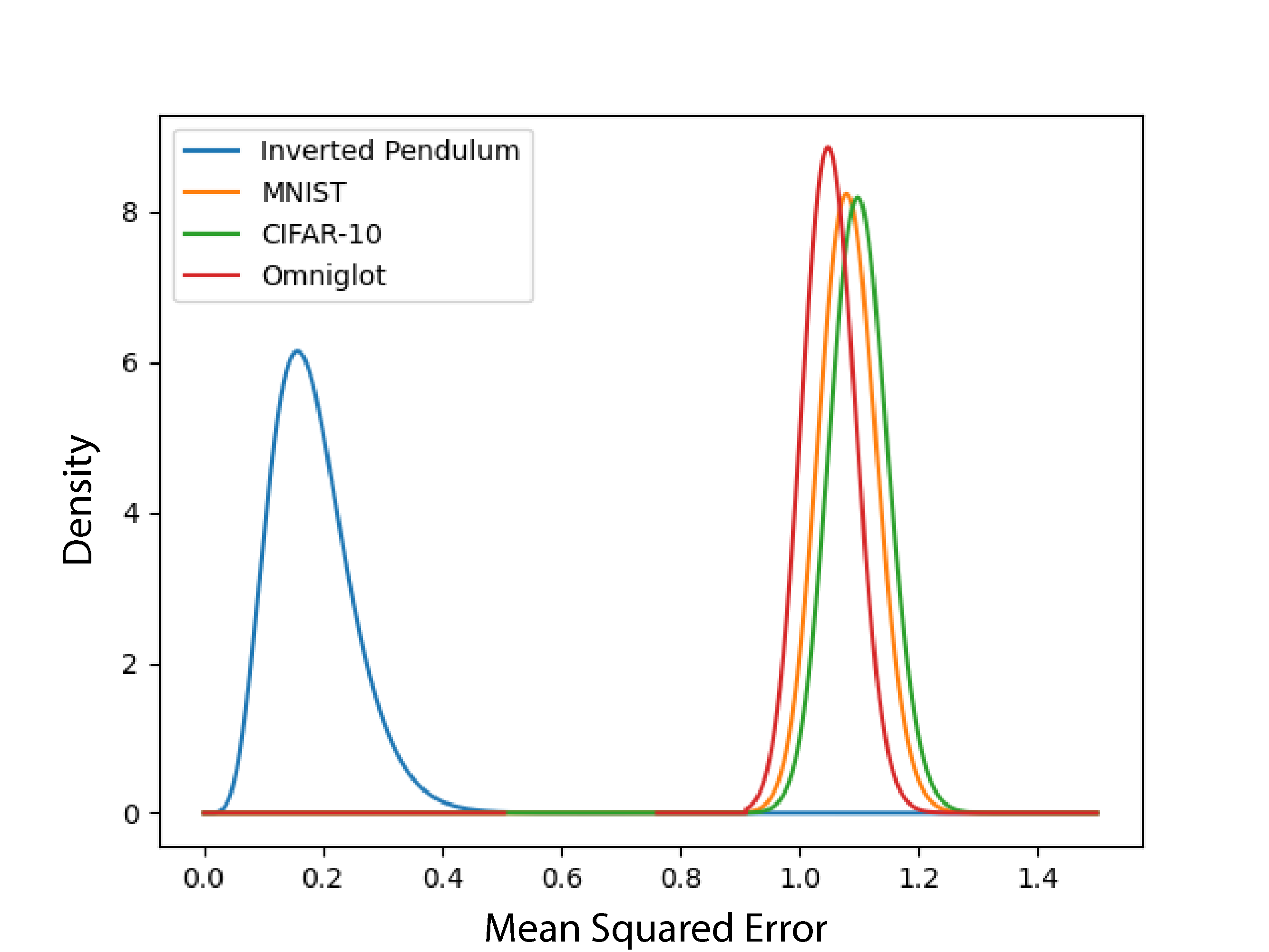
Our evaluation includes benchmark tasks across various domains: MNIST Lecun et al. (1998), CIFAR-10 Krizhevsky et al. (2009), 5-way 1-shot Omniglot Lake et al. (2015) and inverted pendulum control Florian (2007). We treat classification tasks as regression problems using mean squared error loss with one-hot-encoded labels. Two hypothesis spaces are examined: a Gaussian RBF kernel-based space and a high-capacity ReLU-activated neural network.

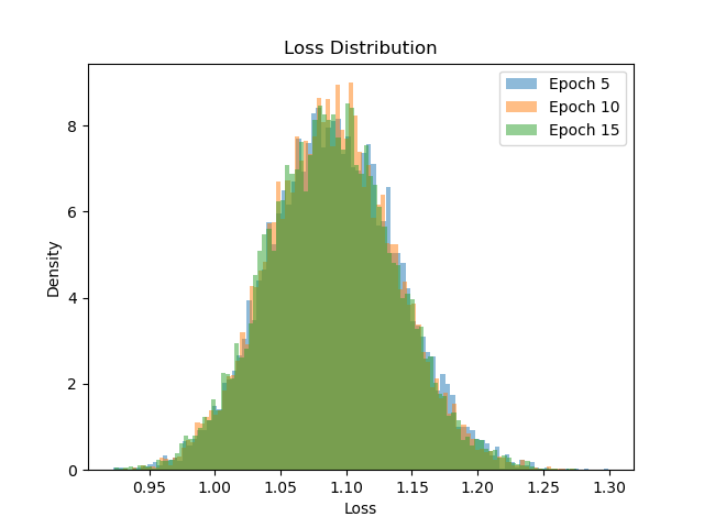
The kernel-based hypothesis space uses a Gaussian RBF kernel constructed as $K(x_{1},x_{2})=e^{-\frac{1}{2}||x_{1}-x_{2}||_{2}^{2}I}$. Hypotheses from this space are constrained to fit the training data; thus, our inductive bias measure quantifies additional information required to generalize on top of the training data. We use Algorithm 1 to sample hypotheses from this space and evaluate their mean squared error on the test set of each task. Note that this hypothesis space is infinite-dimensional; directly optimizing in the space is not feasible. Due to computational constraints, gradient descent in Algorithm 1 is not run until full convergence; thus, sampled hypotheses may not interpolate the training data. Nevertheless, we find that the corresponding distribution of losses stabilizes after a small number of epochs (see the Appendix).

	Linear	FC	Deep CNN	Alexnet	LeNet-5	DSN	MCDNN	DenseNet
MNIST	0.0	0.0	-	0.0	0.0	0.3	7.7	-
CIFAR-10	0.0	0.0	-	0.0	-	0.0	0.0	7.2
SVHN	-	0.0	345.7	67.5	-	405.6	-	507.1
	Matching Nets	MAML	Prototypical Nets	iMAML	MT-net
Omniglot	1400	1700	1800	2500	2500

Table 2: Inductive bias (in bits) of various combinations of models and datasets under a neural network hypothesis space. Inductive bias of models is assessed using error rates reported in prior literature Lecun et al. (1998); Mrgrhn (2021); Lee et al. (2015); Ciregan et al. (2012); Nishimoto (2018); Lin et al. (2015); Krizhevsky et al. (2012); Huang et al. (2017); Mauch and Yang (2017); Veeramacheneni et al. (2022); Goodfellow et al. (2013); Finn et al. (2017); Rajeswaran et al. (2019); Vinyals et al. (2016); Snell et al. (2017); Lee and Choi (2018). - indicates that results are not available in prior literature.

Second, we consider the hypothesis space expressible by a high-capacity ReLU-activated fully-connected neural network with $9$ layers and $512$ units per hidden layer. The appendix describes the details of how the hypothesis space is constructed. We sample hypotheses from this space by training networks of this architecture under different random initialization and training data permutations. For both spaces, we fit a Chi-squared distribution to the distribution of test errors to compute inductive bias (Section 3.3). The appendix includes further experimental details.

Table 1 shows our inductive bias estimates and compares them to Boopathy et al. (2023)’s prior upper bounds on the inductive bias; Boopathy et al. (2023) use a similarly high-dimensional hypothesis space as our kernel-based hypothesis space. Under both our hypothesis spaces, our measure is many orders of magnitude lower than Boopathy et al. (2023)’s prior upper bound. This is because Boopathy et al. (2023) computed upper bounds of inductive bias, while we used a more precise estimation method. Further, our hypothesis space, although quite broad, is different than theirs and potentially more restricted, leading to fewer bits being needed to narrow down the well-generalizing hypotheses.

We also see that tasks with more intrinsic dimensionality require more bits of inductive bias to generalize well; in particular, Inverted Pendulum $<$ MNIST $<$ CIFAR-10 $<$ Omniglot, which matches expectations from Boopathy et al. (2023). Moreover, under the neural network hypothesis space, the required inductive bias is lower than for the kernel hypothesis space, especially for the simpler tasks; for all tasks but Omniglot, the inductive bias is roughly an order of magnitude lower. Thus, neural networks provide a strong bias compared to kernels for these tasks. On the other hand, since Omniglot is a few-shot learning task, plain neural networks provide limited inductive bias for it relative to kernels. Specialized few-shot learning methods include the inductive bias that the output should relate to the query input in the same way that the training labels relate to the training inputs: in other words, they know the analogical structure of the task. Plain neural networks do not contain this information, and thus carry limited inductive bias in this setting.

4.2 Inductive Bias in Different Models

Next, we evaluate the amount of inductive bias contained by different models. Note that our inductive bias measure is a function of the desired test set error rate ($\varepsilon$ in Equation 1); previously, we set the desired error rate as a fixed value for each task. However, following Boopathy et al. (2023), we may also compute the inductive bias provided by different models by evaluating the test set error of the models and plugging this error into $\varepsilon$ in Equation 1. The inductive bias provided by a model is the amount of information required to achieve the error rate of the model. We evaluate the inductive bias contained models trained in prior work. We use the high-capacity neural network hypothesis space described previously. Note that the architecture of the model used to construct the hypothesis space may be smaller than some of the architectures we evaluate; nevertheless, we believe the hypothesis space is expressive enough to contain functions sufficiently close to the trained models in prior literature. See the appendix for additional evaluation details.

In Table 2, we find that the inductive bias provided by different models trained on the same task is similar. Intuitively, this is because for models to generalize similarly, they must provide similar levels of inductive bias. We also observe that the inductive bias of several simple models is $0$ bits. This corresponds to random models in the hypothesis space outperforming the evaluated model; thus, no additional information is provided by the inductive biases in the model relative to the hypothesis space.

5 Discussion

Our results reveal that different tasks require different levels of inductive bias, with higher dimensional tasks demanding greater amounts. In particular, with expressive kernel-based hypothesis spaces, the required inductive bias can be higher for high-dimensional tasks such a Omniglot compared to lower-dimensional tasks such as CIFAR-10 even when the lower-dimensional task may be intuitively simpler. This curse of dimensionality occurs due to an exponential explosion of the size of the hypothesis space with the task dimension: intuitively, each additional dimension of variation in a task increases the dimensionality of the hypothesis space by a constant factor. Our findings confirm previous research and highlight the importance of the choice of model class, particularly for high-dimensional problems.

We also find that neural networks as a model class, inherently encode large amounts of inductive bias. The choice of neural networks themselves provides a much greater inductive bias than specific architectural choices, although our measure also reveals that architectural choices can provide significant inductive bias. This observation suggests that the strong smoothness Li et al. (2018) and compositionality Mhaskar et al. (2017) constraints of neural networks align well with the properties of realistic tasks. Consequently, these models naturally embody the inductive bias required for a wide range of tasks, underscoring their prevalence and success across various domains.

We note that our empirical results are restricted to two specific choices of hypothesis spaces: a Gaussian RBF kernel-based hypothesis space and a fixed neural network hypothesis space. However, our approach is applicable to general hypothesis spaces. For instance, neural network hypothesis spaces may be constructed in alternate ways than optimization by gradient descent. For instance, we may train a single neural network with dropout, then drop out different sets of nodes in the network with each set corresponding to a sample from the hypothesis space. Future work may be able to extend our inductive bias quantification to these settings.

We propose two potential ways of using our inductive bias quantification. First, it provides an information-theoretic interpretation of the advantages of particular model architectures for specific tasks. By quantifying the amount of inductive bias associated with different architectural choices, researchers can gain insights into how specific design decisions affect the model’s ability to generalize. This understanding helps identify which architectural features contribute most significantly to improved performance and informs the development of more tailored and task-specific models.

Second, the inductive bias measure serves as a quantitative guide for developing tasks that require greater inductive bias. By precisely estimating the amount of inductive bias needed for a given task, researchers can intentionally design challenging benchmarks that push the boundaries of machine learning capabilities. We hope this can encourage the development of more powerful model architectures and learning algorithms that drive the field forward.

Appendix A Proof of Theorem 1

Proof.

Denote the probability distribution over $\mathbb{E}_{x\sim p_{x}}[L(h,x)]$ when $h$ is drawn from $p_{h}$ as $p_{l}(l)$. From the definition of $\tilde{I}$ and $I(\varepsilon,p_{h},p_{x},L)$, it is known that:

$$|\tilde{I}-I(\varepsilon,p_{h},p_{x},L)|=|-\log\int_{-\infty}^{\varepsilon}f(l;\alpha^{*})dl+\log\int_{-\infty}^{\varepsilon}p_{l}(l)dl|$$ (18)

Expressing the difference of logs as a log of a ratio:

$$|\tilde{I}-I(\varepsilon,p_{h},p_{x},L)|=\left|-\log\frac{\int_{-\infty}^{\varepsilon}f(l;\alpha^{*})dl}{\int_{-\infty}^{\varepsilon}p_{l}(l)dl}\right|$$ (19)

Observe that this expression can be upper bounded by:

$$\max_{l}|\log f(l;\alpha^{*})-\log p_{l}(l)|$$ (20)

To see this, denote $k=\max_{l}|\log f(l;\alpha^{*})-\log p_{l}(l)|$. Then,

$$f(l;\alpha^{*})\leq e^{k}p_{l}(l)$$ (21)

This implies:

$$\log\frac{\int_{-\infty}^{\varepsilon}f(l;\alpha^{*})dl}{\int_{-\infty}^{\varepsilon}p_{l}(l)dl}\leq\log\frac{\int_{-\infty}^{\varepsilon}e^{k}p_{l}(l)dl}{\int_{-\infty}^{\varepsilon}p_{l}(l)dl}=\log e^{k}\frac{\int_{-\infty}^{\varepsilon}p_{l}(l)dl}{\int_{-\infty}^{\varepsilon}p_{l}(l)dl}=k$$ (22)

Similarly, $-\log\frac{\int_{-\infty}^{\varepsilon}f(l;\alpha^{*})dl}{\int_{-\infty}^{\varepsilon}p_{l}(l)dl}$ can be upper bounded by $k$. Thus,

$$|\tilde{I}-I(\varepsilon,p_{h},p_{x},L)|\leq\max_{l}|\log f(l;\alpha^{*})-\log p_{l}(l)|$$ (23)

We can upper bound the absolute value as:

$$\max_{l}|\log f(l;\alpha^{*})-\log p_{l}(l)|\leq\max_{l}|\log f(l;\alpha^{*})-\log q_{l}(l)|+\max_{l}|\log q_{l}(l)-\log p_{l}(l)|$$ (24)

We first bound the first term. Reparameterizing $f$ in terms of moments $\mu$:

$$\max_{l}|\log f(l;\alpha^{*})-\log q_{l}(l)|=\max_{l}|\log\tilde{f}(l;\mu^{*})-\log q_{l}(l)|$$ (25)

where $\mu^{*}$ are moment estimates computed as sample averages. We upper bound the absolute value as:

$$\max_{l}|\log\tilde{f}(l;\mu^{*})-\log q_{l}(l)|\leq\max_{l}|\log\tilde{f}(l;\mu^{*})-\log\tilde{f}(l;\bar{\mu})|+\max_{l}|\log\tilde{f}(l;\bar{\mu})-\log q_{l}(l)|$$ (26)

Note that $\max_{l}|\log\tilde{f}(l;\bar{\mu})-\log q_{l}(l)|$ is bounded by $\xi_{l}$. Since $f$ has bounded support, by Hoeffding’s inequality, the deviation from the mean of a single element of $\mu^{*}$ can be bounded as:

$$P(|\mu_{i}^{*}-\bar{\mu}_{i}|^{2}\geq\frac{t}{r})\leq 2e^{-C\frac{n^{2}t}{r}}$$ (27)

for some constant $C$. Using the union bound:

$$P(||\mu_{i}^{*}-\bar{\mu}_{i}||^{2}\geq t)\leq 2re^{-C\frac{n^{2}t}{r}}$$ (28)

We set $\sigma=2re^{-C\frac{n^{2}t}{r}}$, which yields:

$$t=\frac{r}{Cn^{2}}\log\frac{2r}{\sigma}$$ (29)

Thus, with probability $1-\sigma$:

$$P(||\mu_{i}^{*}-\bar{\mu}_{i}||\leq\frac{1}{n}\sqrt{\frac{r}{C}\log\frac{2r}{\sigma}})$$ (30)

Since $\log\tilde{f}$ is Lipschitz continuous with respect to $\mu$, with probability $1-\sigma$:

$$\max_{l}|\log\tilde{f}(l;\mu^{*})-\log\tilde{f}(l;\bar{\mu})|\leq\frac{\kappa}{n}\sqrt{r\log\frac{2r}{\sigma}}$$ (31)

for some constant $\kappa$. Thus, we may bound $\max_{l}|\log f(l;\alpha^{*})-\log q_{l}(l)|$ as:

$$\max_{l}|\log f(l;\alpha^{*})-\log q_{l}(l)|\leq\xi_{l}+\frac{\kappa}{n}\sqrt{r\log\frac{2r}{\sigma}}$$ (32)

Next, we bound $\max_{l}|\log q_{l}(l)-\log p_{l}(l)|$ using the bound on $\max_{h}|\log q_{h}(h)-\log p_{h}(h)|$. Note that

$$\log q_{l}(l)-\log p_{l}(l)=\log\frac{\int_{h:\mathbb{E}_{x\sim p_{x}}[L(h,x)]=l}q_{h}(h)dh}{\int_{h:\mathbb{E}_{x\sim p_{x}}[L(h,x)]=l}p_{h}(h)dh}\leq\log\frac{\int_{h:\mathbb{E}_{x\sim p_{x}}[L(h,x)]=l}e^{\xi_{h}}p_{h}(h)dh}{\int_{h:\mathbb{E}_{x\sim p_{x}}[L(h,x)]=l}p_{h}(h)dh}=\xi_{h}$$ (33)

Similarly,

$$\log p_{l}(l)-\log q_{l}(l)=\log\frac{\int_{h:\mathbb{E}_{x\sim p_{x}}[L(h,x)]=l}p_{h}(h)dh}{\int_{h:\mathbb{E}_{x\sim p_{x}}[L(h,x)]=l}q_{h}(h)dh}\leq\log\frac{\int_{h:\mathbb{E}_{x\sim p_{x}}[L(h,x)]=l}e^{\xi_{h}}q_{h}(h)dh}{\int_{h:\mathbb{E}_{x\sim p_{x}}[L(h,x)]=l}q_{h}(h)dh}=\xi_{h}$$ (34)

Therefore,

$$\max_{l}|\log q_{l}(l)-\log p_{l}(l)|\leq\xi_{h}$$ (35)

Combining all the inequalities, with probability $1-\sigma$:

$$|\tilde{I}-I(\varepsilon,p_{h},p_{x},L)|\leq\xi_{h}+\xi_{l}+\frac{\kappa}{n}\sqrt{r\log\frac{2r}{\sigma}}$$ (36)

∎

Appendix B Additional Experimental Details

B.1 Kernel-based Sampling Details

Using the decomposition of $\theta$, $h(\bar{X})\in\mathbb{R}^{nk}$ can be expressed as:

$$h(\bar{X})=\phi(\bar{X})\phi(X)^{\dagger}Y+\phi(\bar{X})\beta$$ (37)

where $\phi(\bar{X})\in\mathbb{R}^{nk\times P}$. Note that this is distributed as a Gaussian with mean $\phi(\bar{X})\phi(X)^{\dagger}Y$ and covariance matrix $\phi(\bar{X})(I-\phi(X)^{\dagger}\phi(X))\phi(\bar{X})^{T}=\phi(\bar{X})\phi(\bar{X})^{T}-\phi(\bar{X})\phi(X)^{\dagger}\phi(X)\phi(\bar{X})^{T}$. We may express these quantities in terms of the kernel corresponding to features $\phi(x)$. The kernel is defined a $k\times k$ matrix:

$$K(x_{1},x_{2})=\phi(x_{1})\phi(x_{2})^{T}$$ (38)

In our experiments, we use a Gaussian radial basis function (RBF) kernel. We denote $K(X,X)\in\mathbb{R}^{Nk,Nk}$ and $K(\bar{X},X)\in\mathbb{R}^{nK,Nk}$ as the kernels between all pairs of training points and pairs of test and training points respectively. Then, assuming $N<P$, $h(\bar{X})$ has mean $K(\bar{X},X)K(X,X)^{-1}Y$ and covariance $K(\bar{X},\bar{X})-K(\bar{X},X)K(X,X)^{-1}K(X,\bar{X})$. Thus, we may express $h(\bar{X})$ as:

$$h(\bar{X})=K(\bar{X},X)K(X,X)^{-1}Y+\sqrt{K(\bar{X},\bar{X})-K(\bar{X},X)K(X,X)^{-1}K(X,\bar{X})}z$$ (39)

where $z\in\mathbb{R}^{nk}$ is distributed as a unit Gaussian and $\sqrt{}$ denotes matrix square root. Computing this quantity directly for a given choice of $z$ may be computationally challenging since it requires storing and inverting the kernel matrix $K(X,X)$. Thus, we instead approximate solutions to $K(X,X)^{-1}Y$ and $K(X,X)^{-1}K(X,\bar{X})$ via gradient descent. Specifically, we define $\alpha^{*}=K(X,X)^{-1}Y$ and $A^{*}=K(X,X)^{-1}K(X,\bar{X})$. Note that these can be found as solutions to the following optimization problems:

$$\alpha^{*}=\operatorname*{arg\,min}_{\alpha}||Y-K(X,X)\alpha||_{2}^{2}$$ (40)

$$A^{*}=\operatorname*{arg\,min}_{A}||K(X,\bar{X})-K(X,X)A||_{F}^{2}$$ (41)

We find approximate solutions to these optimization problems by stochastic gradient descent. Once $\alpha^{*}$ and $A^{*}$ are found, samples of $h(\bar{X})$ may be computed as:

$$h(\bar{X})=K(\bar{X},X)\alpha^{*}+\sqrt{K(\bar{X},\bar{X})-K(\bar{X},X)A^{*}}z$$ (42)

Assuming a constant time kernel computation per element, performing stochastic gradient descent on $\alpha$ and $A$ for one iteration requires $O(Nk)$ and $O(nNk^{2})$ time respectively; thus, for $T$ optimization steps, the time complexity is $O(nNk^{2}T)$. Once computed, sampling $h(\bar{X})$ requires $O(n^{3}k^{3}+n^{2}Nk^{3})$ time to determine the constants in the above equation, and an additional $O(n^{2}k^{2})$ per sample. Thus, producing $S$ samples requires a total of $O(nNk^{2}T+n^{3}k^{3}+n^{2}Nk^{3}+n^{2}k^{2}S)$ time. Importantly, this time is linear in the training set size and constant in the parameter size; this efficiency is critical for large datasets and high-dimensional hypothesis spaces.

Figure 4: Distribution of hypothesis losses for MNIST after 5, 10, and 15 epochs of gradient descent. Notice that the update in distribution is minimal.

We use a Gaussian RBF kernel constructed as $K(x_{1},x_{2})=e^{-\frac{1}{2}||x_{1}-x_{2}||_{2}^{2}I}$. Due to the computational cost of computing the full gradients $g_{\alpha}$ and $g_{A}$ (both of which have sizes scaling linearly with the training set size), we compute the gradient in steps. Specifically, for $g_{\alpha}$, $K(x,X)\alpha$ is computed by splitting the training set into groups $X_{i}$ (and correspondingly $\alpha$ into $\alpha_{i}$) and summing the contribution of each $K(x,X_{i})\alpha_{i}$. An analogous grouping is done to compute $g_{A}$.

For experiments on MNIST, we use a learning rate of $0.0001$ to optimize $\alpha$ and a learning rate of $0.00001$ to optimize $A$. We use a batch size of $128$ and a group size of $2048$. Training is performed for $20$ epochs. See Figure 4 for an analysis of the convergence of the resulting loss distribution.

For experiments on CIFAR-10, we use a learning rate of $0.001$ to optimize $\alpha$ and a learning rate of $0.0001$ to optimize $A$. We use a batch size of $64$ and a group size of $1024$. Training is performed for $20$ epochs.

For experiments on Omniglot, we use a learning rate of $0.0001$ to optimize $\alpha$ and a learning rate of $0.00001$ to optimize $A$. We use a batch size of $10$ and a group size of $100$. Training is performed for $1$ epoch.

For experiments on the inverted pendulum task, we use a learning rate of $0.001$ to optimize $\alpha$ and a learning rate of $0.0001$ to optimize $A$. We use a batch size of $64$ and a group size of $1024$. Training is performed for $500$ epochs.

For the kernel-based hypothesis space, we sample a total of $100000$ hypotheses in each setting.

B.2 Neural Network Hypothesis Space Details

The architecture of our base hypothesis space is constructed as follows: the input is linearly projected to a $512$ dimensional vector, followed by $9$ more fully connected layers of dimensionality $512$. Finally, the output is linearly projected to a $10$-dimensional output to predict the one-hot encoded label. All layers include a bias term. Each fully connected layer except the final one is followed by a ReLU non-linearity. No additional components such as normalization are used.

The model is trained on a mean squared error loss using Adam with a learning rate of $0.001$. Training is conducted for $10$ epochs with a batch size of $128$. We sample $100$ hypotheses from this hypothesis space by using different random initializations and orderings of training points during training.

Within the neural network hypothesis space, we consider the performance of models trained in prior work. Prior work typically reports the test set accuracy of each model; however, our method uses test set mean squared error as an error metric instead since the theoretical prediction of a Chi-squared error distribution is only available for mean-squared error. Thus, we estimate mean squared errors from accuracies by simply setting mean squared error $e$ as $1-a$ where $a$ represents accuracy.

Figure 5: Fitted scaled non-central Chi-squared distributions for the test set errors on MNIST, CIFAR-10, Omniglot, and Inverted Pendulum tasks under a Gaussian RBF kernel hypothesis space.

B.3 Distribution Fitting Details

Given samples from the hypothesis space, compute the test set error for each one. Then, given the empirical distribution of test set errors, we fit a three-parameter scaled non-central Chi-squared distribution to match the data. We use maximum likelihood estimation to determine the fit parameters. Figure 5 illustrates example fitted distributions under the Gaussian RBF kernel hypothesis space. Once the distribution parameters are determined, we use approximations to quantify the log of the cumulative distribution function as described in the main text.

B.4 Tasks

For all tasks, desired error rates are set as the values provided in Boopathy et al. [2023] unless otherwise specified.

MNIST & CIFAR-10

We use the base MNIST and CIFAR-10 datasets without modification.

ImageNet

We use standard ImageNet normalization and random cropping.

Omniglot

We consider 5-way 1-shot Omniglot classification. In this setting, each input consists of $5$ images, $1$ from each of $5$ alphabets, and the goal is to predict the class of a new image from one of the $5$ seen alphabets. We encode this task in the following form: the inputs $x$ consist of $6$ images, the first $5$ of which correspond to training images and the last one of which corresponds to the evaluation image. The input is flattened to remove all spatial structure. The desired output is a one-hot encoded $5$-dimensional vector of which of the $5$ training images matches the class of the evaluation image. We generate a training set of size $10000$ and a test set of size $100$, drawn from the Omniglot background and evaluation alphabets respectively.

Inverted Pendulum Task

We consider the following inverted pendulum control task: an inverted pendulum with angle $\theta\in\mathbb{R}$ and angular velocity $\omega\in\mathbb{R}$ has the following dynamics:

$$\dot{\theta}=\omega$$ (43)

$$\dot{\omega}=\sin\theta+u$$ (44)

where $u\in\mathbb{R}$ is a control action. The goal is to minimize the time average of the following cost:

$$C(u,\theta,\omega)=\frac{1}{2}u^{2}+24\theta^{2}+(8\theta+4\omega)(\theta-\sin\theta)$$ (45)

The first term encourages small control actions. The second term encourages the inverted pendulum to remain at rest at $\theta=0$. The third term is added to allow an analytically tractable optimal control. Intuitively, it penalizes when future values of $\theta$ (as represented by $8\theta+4\omega$) are far from $0$ (as represented by $\theta-\sin\theta$). Note that this term is on the order of $O(\theta^{3})$; for small $\theta$, the second term dominates.

The optimal cost to go, or value function (i.e. the optimal total cost over all future time steps) given current state $\theta,\omega$ is:

$$V(\theta,\omega)=14\theta^{2}+8\theta\omega+2\omega^{2}$$ (46)

To verify this, note that the optimal cost obeys the Bellman equation:

$$\min_{u}\frac{\partial}{\partial\theta}V(\theta,\omega)\dot{\theta}+\frac{\partial}{\partial\omega}V(\theta,\omega)\dot{\omega}+C(u,\theta,\omega)=0$$ (47)

Substituting in the expressions from above:

$$\min_{u}[(28\theta+8\omega)\omega+(8\theta+4\omega)(\sin\theta+u)+\frac{1}{2}u^{2}+24\theta^{2}+(8\theta+4\omega)(\theta-\sin\theta)]=0$$ (48)

Setting the derivative with respect to $u$ to $0$, the optimal $u$ must satisfy:

$$8\theta+4\omega+u=0$$ (49)

Thus, $u=-8\theta-4\omega$. Plugging this back into the Bellman equation:

$$(28\theta+8\omega)\omega+(8\theta+4\omega)(\sin\theta-8\theta-4\omega)+\frac{1}{2}(-8\theta-4\omega)^{2}+24\theta^{2}+(8\theta+4\omega)(\theta-\sin\theta)=0$$ (50)

Observe that all terms on the left-hand side cancel; thus $V(\theta,w)$i is the correct value function for this optimal control problem. Given $\theta,\omega$, the optimal control action is:

$$u=-8\theta-4\omega$$ (51)

In this task, inputs $(\theta,\omega)$ are drawn from a uniform distribution over $[-\pi,\pi]\times[-1,1]$. Desired outputs $u$ are constructed as above. We generate a training set of size $10000$ and a test set of size $100$.

B.5 Computing Infrastructure

Experiments are run on a computing cluster with GPUs ranging in memory size from 11 GB to 80 GB.

References

- Amari [1993] Shunichi Amari. A universal theorem on learning curves. Neural Networks, 6(2):161–166, 1993.
- Bahri et al. [2021] Yasaman Bahri, Ethan Dyer, Jared Kaplan, Jaehoon Lee, and Utkarsh Sharma. Explaining neural scaling laws. arXiv preprint arXiv:2102.06701, 2021.
- Blumer et al. [1989] Anselm Blumer, A. Ehrenfeucht, David Haussler, and Manfred K. Warmuth. Learnability and the vapnik-chervonenkis dimension. J. ACM, 36(4):929–965, oct 1989.
- Boopathy et al. [2023] Akhilan Boopathy, Kevin Liu, Jaedong Hwang, Shu Ge, Asaad Mohammedsaleh, and Ila Fiete. Model-agnostic measure of generalization difficulty. ICML, 2023.
- Chollet [2019] François Chollet. On the measure of intelligence. arXiv preprint, 2019.
- Ciregan et al. [2012] Dan Ciregan, Ueli Meier, and Jürgen Schmidhuber. Multi-column deep neural networks for image classification. In CVPR, 2012.
- Cortes et al. [1994] Corinna Cortes, L. D. Jackel, Sara Solla, Vladimir Vapnik, and John Denker. Learning curves: Asymptotic values and rate of convergence. In NeurIPS, 1994.
- Deng et al. [2009] Jia Deng, Wei Dong, Richard Socher, Li-Jia Li, Kai Li, and Li Fei-Fei. ImageNet: A large-scale hierarchical image database. In CVPR, 2009.
- Du et al. [2018] Simon S. Du, Yining Wang, Xiyu Zhai, Sivaraman Balakrishnan, Ruslan Salakhutdinov, and Aarti Singh. How many samples are needed to estimate a convolutional or recurrent neural network? NeurIPS, 2018.
- Finn et al. [2017] Chelsea Finn, Pieter Abbeel, and Sergey Levine. Model-agnostic meta-learning for fast adaptation of deep networks. In ICML, pages 1126–1135. PMLR, 2017.
- Florian [2007] Razvan V Florian. Correct equations for the dynamics of the cart-pole system. Center for Cognitive and Neural Studies (Coneural), Romania, 2007.
- Goodfellow et al. [2013] Ian J Goodfellow, Yaroslav Bulatov, Julian Ibarz, Sacha Arnoud, and Vinay Shet. Multi-digit number recognition from street view imagery using deep convolutional neural networks. arXiv preprint arXiv:1312.6082, 2013.
- Haussler [1988] David Haussler. Quantifying inductive bias: Ai learning algorithms and valiant’s learning framework. Artificial Intelligence, 36(2):177–221, 1988.
- Hernández-Orallo [2016] José Hernández-Orallo. Evaluation in artificial intelligence: from task-oriented to ability-oriented measurement. Artificial Intelligence Review, Aug 2016.
- Hestness et al. [2017] Joel Hestness, Sharan Narang, Newsha Ardalani, Gregory Diamos, Heewoo Jun, Hassan Kianinejad, Md. Mostofa Ali Patwary, Yang Yang, and Yanqi Zhou. Deep learning scaling is predictable, empirically. arXiv preprint, 2017.
- Huang et al. [2017] Gao Huang, Zhuang Liu, Laurens Van Der Maaten, and Kilian Q Weinberger. Densely connected convolutional networks. In CVPR, 2017.
- Hutter [2021] Marcus Hutter. Learning curve theory. arXiv preprint arXiv:2102.04074, 2021.
- Jiang et al. [2021] Yiding Jiang, Parth Natekar, Manik Sharma, Sumukh K Aithal, Dhruva Kashyap, Natarajan Subramanyam, Carlos Lassance, Daniel M Roy, Gintare Karolina Dziugaite, Suriya Gunasekar, et al. Methods and analysis of the first competition in predicting generalization of deep learning. In NeurIPS 2020 Competition and Demonstration Track, 2021.
- Kawaguchi et al. [2022] Kenji Kawaguchi, Zhun Deng, Kyle Luh, and Jiaoyang Huang. Robustness implies generalization via data-dependent generalization bounds. In ICML, 2022.
- Koltchinskii and Panchenko [2000] Vladimir Koltchinskii and Dmitriy Panchenko. Rademacher processes and bounding the risk of function learning. High Dimensional Probability II, page 443–457, 2000.
- Krizhevsky et al. [2009] Alex Krizhevsky, Vinod Nair, and Geoffrey Hinton. Cifar-10 and cifar-100 datasets. 2009.
- Krizhevsky et al. [2012] Alex Krizhevsky, Ilya Sutskever, and Geoffrey E Hinton. Imagenet classification with deep convolutional neural networks. In NeurIPS, 2012.
- Lake et al. [2015] B. Lake, R. Salakhutdinov, and J. Tenenbaum. Human-level concept learning through probabilistic program induction. Science, 350:1332 – 1338, 2015.
- Lecun et al. [1998] Y. Lecun, L. Bottou, Y. Bengio, and P. Haffner. Gradient-based learning applied to document recognition. Proceedings of the IEEE, 86(11):2278–2324, 1998.
- Lee and Choi [2018] Yoonho Lee and Seungjin Choi. Gradient-based meta-learning with learned layerwise metric and subspace. In ICML, pages 2927–2936. PMLR, 2018.
- Lee et al. [2015] Chen-Yu Lee, Saining Xie, Patrick Gallagher, Zhengyou Zhang, and Zhuowen Tu. Deeply-supervised nets. In AISTATS, 2015.
- Lei et al. [2015] Yunwen Lei, Urun Dogan, Alexander Binder, and Marius Kloft. Multi-class svms: From tighter data-dependent generalization bounds to novel algorithms. NeurIPS, 2015.
- Li et al. [2018] Hao Li, Zheng Xu, Gavin Taylor, Christoph Studer, and Tom Goldstein. Visualizing the loss landscape of neural nets. NeurIPS, 2018.
- Li et al. [2021] Zhiyuan Li, Yi Zhang, and Sanjeev Arora. Why are convolutional nets more sample-efficient than fully-connected nets? ICLR, 2021.
- Lin et al. [2015] Zhouhan Lin, Roland Memisevic, and Kishore Konda. How far can we go without convolution: Improving fully-connected networks. arXiv preprint, 2015.
- Lin et al. [2023] Jihao Andreas Lin, Javier Antorán, Shreyas Padhy, David Janz, José Miguel Hernández-Lobato, and Alexander Terenin. Sampling from gaussian process posteriors using stochastic gradient descent. arXiv preprint, 2023.
- Mauch and Yang [2017] Lukas Mauch and Bin Yang. A novel layerwise pruning method for model reduction of fully connected deep neural networks. In ICASSP, 2017.
- Mhaskar et al. [2017] Hrushikesh Mhaskar, Qianli Liao, and Tomaso Poggio. When and why are deep networks better than shallow ones? In AAAI, 2017.
- Mrgrhn [2021] Guido Mrgrhn. Alexnet with tensorflow, 2021.
- Murata et al. [1992] Noboru Murata, Shuji Yoshizawa, and Shun-ichi Amari. Learning curves, model selection and complexity of neural networks. In NeurIPS, 1992.
- Negrea et al. [2019] Jeffrey Negrea, Mahdi Haghifam, Gintare Karolina Dziugaite, Ashish Khisti, and Daniel M Roy. Information-theoretic generalization bounds for sgld via data-dependent estimates. NeurIPS, 2019.
- Nishimoto [2018] Bruno Eidi Nishimoto. Linear classifier, 2018.
- Raginsky et al. [2016] Maxim Raginsky, Alexander Rakhlin, Matthew Tsao, Yihong Wu, and Aolin Xu. Information-theoretic analysis of stability and bias of learning algorithms. In IEEE Information Theory Workshop (ITW), 2016.
- Rajeswaran et al. [2019] Aravind Rajeswaran, Chelsea Finn, Sham M Kakade, and Sergey Levine. Meta-learning with implicit gradients. NeurIPS, 32, 2019.
- Sankaran [1959] Munuswamy Sankaran. On the non-central chi-square distribution. Biometrika, 46(1/2):235–237, 1959.
- Sharma and Kaplan [2022] Utkarsh Sharma and Jared Kaplan. Scaling laws from the data manifold dimension. JMLR, 23:9–1, 2022.
- Snell et al. [2017] Jake Snell, Kevin Swersky, and Richard Zemel. Prototypical networks for few-shot learning. NeurIPS, 30, 2017.
- Veeramacheneni et al. [2022] Lokesh Veeramacheneni, Moritz Wolter, Reinhard Klein, and Jochen Garcke. Canonical convolutional neural networks. arXiv preprint arXiv:2206.01509, 2022.
- Vinyals et al. [2016] Oriol Vinyals, Charles Blundell, Timothy Lillicrap, Daan Wierstra, et al. Matching networks for one shot learning. NeurIPS, 29, 2016.
- Wolpert [1996] David H Wolpert. The lack of a priori distinctions between learning algorithms. Neural computation, 8(7):1341–1390, 1996.