The Perils of Optimizing Learned Reward Functions: Low Training Error Does Not Guarantee Low Regret

Abstract

In reinforcement learning, specifying reward functions that capture the intended task can be very challenging. Reward learning aims to address this issue by learning the reward function. However, a learned reward model may have a low error on the training distribution, and yet subsequently produce a policy with large regret. We say that such a reward model has an error-regret mismatch. The main source of an error-regret mismatch is the distributional shift that commonly occurs during policy optimization. In this paper, we mathematically show that a sufficiently low expected test error of the reward model guarantees low worst-case regret, but that for any fixed expected test error, there exist realistic data distributions that allow for error-regret mismatch to occur. We then show that similar problems persist even when using policy regularization techniques, commonly employed in methods such as RLHF. Our theoretical results highlight the importance of developing new ways to measure the quality of learned reward models.

1 Introduction

To solve a sequential decision problem with reinforcement learning (RL), we must first formalize that decision problem using a reward function (Sutton and Barto, 2018). However, for complex tasks, reward functions are often hard to specify correctly. To solve this problem, it is increasingly popular to learn reward functions with reward learning algorithms, instead of specifying the reward functions manually. There are many different reward learning algorithms (e.g., Ng and Russell, 2000; Tung et al., 2018; Brown and Niekum, 2019; Palan et al., 2019), with one of the most popular being reward learning from human feedback (RLHF) (Christiano et al., 2017; Ibarz et al., 2018).

For any learning algorithm, it is a crucial question whether or not that learning algorithm is guaranteed to converge to a “good” solution. For example, in the case of supervised learning for classification, it can be shown that a learning algorithm that produces a model with a low empirical error (i.e., training error) is likely to have a low expected error (i.e., test error), given a sufficient amount of training data and assuming that both the training data and the test data is drawn i.i.d. from a single stationary distribution (Kearns and Vazirani, 1994). In the case of normal supervised learning, we can therefore be confident that a learning algorithm will converge to a good model, provided that it is given a sufficient amount of training data (under some standard assumptions).

However, reward learning is different from normal supervised learning in several important aspects. First of all, the fact that a machine learning model has a low training error only ensures that it is accurate relative to the training distribution. However, when we do reward learning, we want to learn a reward function that produces good policies if that reward function is optimized. Moreover, such optimization effectively corresponds to a form of distributional shift. This raises the worry that a learned reward function might fail to produce good policies, even if it is highly accurate on the training distribution (since a model in general can be accurate on a training distribution, without being accurate after distributional shift). Stated differently, a low training error only requires that the true reward function and the learned reward function are similar in the training distribution, whereas robustness to policy optimization requires the two reward functions to have similar optimal policies. Prima facie, it does not seem as though these two requirements should be robustly correlated. It is therefore not clear that reward learning algorithms should be guaranteed to converge to good reward functions. If a reward model has both low training error and an optimal policy with large regret, we say that there is an error-regret mismatch. This dynamic is illustrated in Figure 1.

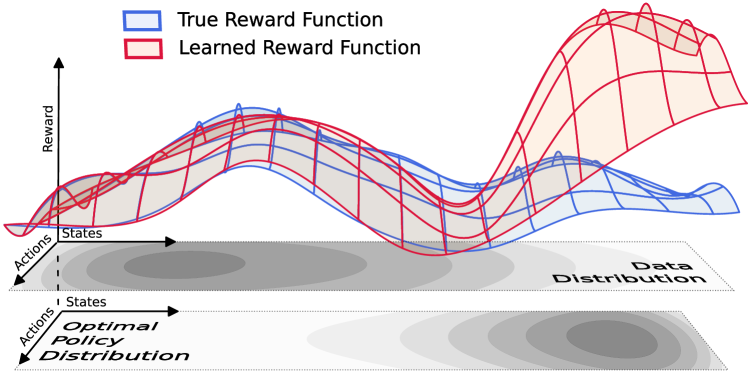
Figure 1: Reward models (red function) are commonly trained in a supervised fashion to approximate some latent, true reward (blue function). This is achieved by sampling reward data (e.g., in the form of preferences over trajectory segments) from some training distribution (upper gray layer) and then learning parameters to minimize the empirical loss on this distribution. Given enough data, this loss will approximate the expected loss to arbitrary precision in expectation. However, low expected loss only guarantees a good approximation to the true reward function in areas with high coverage by the training distribution! On the other hand, optimizing an RL policy to maximize the learned reward model induces a distribution shift which can lead the policy to exploit uncertainties of the learned reward model in low-probability areas of the transition space (lower gray layer). We refer to this phenomenon as error-regret mismatch.

In this paper, we study the relationship between the expected error of a reward model on some data distribution and the extent to which optimizing that reward model is guaranteed to produce a policy with low regret according to the true reward function.

We establish that:

1. As the error of a learned reward model on the training distribution goes to zero, the worst-case regret of optimizing a policy according to that reward model also goes to zero, for any training distribution (Theorem 3.1).

2. However, for any $\epsilon>0$, whenever a training distribution has sufficiently low coverage of some bad policy, there exists a reward model that achieves an expected error of $\epsilon$ but gives rise to error-regret mismatch (Proposition 3.2).

3. More precisely, for every $\epsilon>0$ there is a set of linear constraints (depending on the underlying MDP, and the true reward function) that precisely characterize the training distributions that make error-regret mismatch with an expected error of $\epsilon$ possible (Theorem 3.3).

We then investigate the case of regularized policy optimization (including KL-regularized policy optimization, which is commonly used in methods such as RLHF). We show that:

1. For every training distribution and reference policy, there exists an $\epsilon>0$ such that regularized policy optimization on the learned reward model is guaranteed to yield better performance than the reference policy when the expected error of the reward model is smaller than $\epsilon$. (Theorem 4.1).

2. However, even in the regularized optimization setting, for every $\epsilon>0$, if the training distribution has sufficiently low coverage of some bad policy, there still exists a reward model that makes error-regret mismatch with an expected error of $\epsilon$ possible (Theorem 4.2).

We then develop several generalizations of our results to different types of data sources for reward model training, such as preferences over trajectories (Propositions 5.2 and 5.3), and trajectory scoring (Proposition 5.1). Lastly, we provide a case analysis for RLHF in the mixed bandit case where we provide a more interpretable formulation (Proposition 6.1) of the failure mode discussed in Theorem 4.2 for general MDPs.

Our results thus indicate that reward learning algorithms should be expected to converge to good reward functions in the limit of infinite data. However, low training error does not imply low worst-case regret, because for any non-zero $\epsilon$ there is typically a reward model with error-regret mismatch. Moreover, regularizing the learned policy to be close to the training distribution can mitigate this problem, but will typically not solve it. Our results thus contribute to building up the foundations for the statistical learning theory of reward learning.

1.1 Related work

Reward learning refers to the general idea of learning the reward function used for reinforcement learning, which is especially useful for complex tasks with latent and difficult-to-specify reward functions. Many methods have been developed to incorporate various types of human feedback (Wirth et al., 2017; Ng et al., 2000; Bajcsy et al., 2017; Jeon et al., 2020). However, reward learning presents several challenges (Casper et al., 2023; Lang et al., 2024b; Skalse and Abate, 2023, 2024), such as reward misgeneralization, where the reward model learns a different reward function that performs well in-distribution but differs strongly on out-of-distribution data (Skalse et al., 2023). This can lead to reward hacking (Krakovna, 2020; Skalse et al., 2022), a consequence of Goodhart’s law (Goodhart, 1984; Zhuang and Hadfield-Menell, 2020; Hennessy and Goodhart, 2023; Strathern, 1997; Karwowski et al., 2023). Reward hacking has been extensively studied theoretically Skalse et al. (2022, 2024); Zhuang and Hadfield-Menell (2020) and empirically (Zhang et al., 2018; Farebrother et al., 2018; Cobbe et al., 2019; Krakovna, 2020; Gao et al., 2023; Tien et al., 2022). Our work analyzes the conditions under which a data distribution allows for reward model misgeneralization leading to reward hacking. Some prior works investigate similar failure cases by deriving sample complexity bounds for RLHF and DPO  (Zhu et al., 2024; Nika et al., 2024). In contrast, we investigate safety properties of the data distributions used to train the reward model and focus on a more general class of reward learning methods.

Lastly, several approaches have been proposed to address the issue of out-of-distribution robustness in reward learning, such as ensembles of conservative reward models (Coste et al., 2023), averaging weights of multiple reward models (Ramé et al., 2024), iteratively updating training labels (Zhu et al., 2024), on-policy reward learning (Lang et al., 2024a), and distributionally robust planning (Zhan et al., 2023). Furthermore, in classical machine learning, research in out-of-distribution generalization has a long history, and a rich literature of methods exists  (Li et al., 2022; Zhou et al., 2022; Wang et al., 2022; Liu et al., 2021; Li et al., 2023; Yoon et al., 2023). For reinforcement learning in particular, the issue of distributional shift is of particular importance in offline reinforcement learning  (Prudencio et al., 2023), with many different methods having been developed to address this issue  (Prudencio et al., 2023; Fujimoto et al., 2019; Yu et al., 2021; Kidambi et al., 2020; Chen et al., 2020; Zhang et al., 2020; Janner et al., 2021)

2 Preliminaries

A Markov Decision Process (MDP) is a tuple $\langle\mathcal{S},\mathcal{A},\tau,\mu_{0},R,\gamma\rangle$ where $\mathcal{S}$ is a set of states, $\mathcal{A}$ is a set of actions, $\tau:{\mathcal{S}{\times}\mathcal{A}}\to\Delta(\mathcal{S})$ is a transition function, $\mu_{0}\in\Delta(S)$ is an initial state distribution, $R:{\mathcal{S}{\times}\mathcal{A}}\to\mathbb{R}$ is a reward function, and $\gamma\in(0,1)$ is a discount rate. We define the range of a reward function $R$ as $\mathrm{range}\ R\coloneqq\max_{(s,a)\in{\mathcal{S}{\times}\mathcal{A}}}R(s,a)-\min_{(s,a)\in{\mathcal{S}{\times}\mathcal{A}}}R(s,a)$.

A policy is a function $\pi:\mathcal{S}\to\Delta(\mathcal{A})$. We denote the set of all possible policies by $\Pi$. A trajectory $\xi=\langle s_{0},a_{0},s_{1},a_{1},...\rangle$ is a possible path in an MDP. The return function $G$ gives the cumulative discounted reward of a trajectory, $G(\xi)=\sum_{t=0}^{\infty}\gamma^{t}R(s_{t},a_{t})$, and the evaluation function $J$ gives the expected trajectory return given a policy, $J(\pi)=\mathbb{E}_{\xi\sim\pi}\left[{G(\xi)}\right]$. A policy maximizing $J$ is an optimal policy. We define the regret of a policy $\pi$ with respect to reward function $R$ as $\mathrm{Reg}^{R}\left(\pi\right)\coloneqq\frac{\max J_{R}-J_{R}(\pi)}{\max J_{R}-\min J_{R}}\in[0,1]$. Here, $J_{R}$ is the policy evaluation function for $R$.

In this paper, we assume that $\mathcal{S}$ and $\mathcal{A}$ are finite, and that all states are reachable under $\tau$ and $\mu_{0}$. We also assume that $\max J_{R}-\min J_{R}\neq 0$ (since the reward function would otherwise be trivial). Note that this implies that $\mathrm{range}\ R>0$, and that $\mathrm{Reg}^{R}\left(\pi\right)$ is well-defined.

The state-action occupancy measure is a function $\eta:\Pi\to\mathbb{R}^{|{\mathcal{S}{\times}\mathcal{A}}|}$ mapping each policy $\pi\in\Pi$ to the corresponding "state-action occupancy measure", describing the discounted frequency that each state-action tuple is visited by a policy. Formally, $\eta(\pi)(s,a)=\eta^{\pi}(s,a)=\sum_{t=0}^{\infty}\gamma^{t}\cdot P(s_{t}=s,a_{t}=a\ |\ \xi\sim\pi)$. Note that by writing the reward function $R$ as a vector $\vec{R}\in\mathbb{R}^{|{\mathcal{S}{\times}\mathcal{A}}|}$, we can split $J$ into a function that is linear in $R$: $J(\pi)=\eta^{\pi}\cdot\vec{R}$. By normalizing a state-action occupancy measure $\eta^{\pi}$ we obtain a policy-induced distribution $D^{\pi}\coloneqq(1-\gamma)\cdot\eta^{\pi}$.

2.1 Problem formalization

In RL with reward learning, we assume that we have an MDP $\langle\mathcal{S},\mathcal{A},\tau,\mu_{0},R,\gamma\rangle$ where the reward function $R$ is unknown. We may also assume that $\tau$ and $\mu_{0}$ are unknown, as long as we are able to sample from them (though $\mathcal{S}$, $\mathcal{A}$, and $\gamma$ must generally be known, at least implicitly). We then go through the following steps:

1. We first learn a reward function $\hat{R}$ from data. In practice, a reward learning algorithm may use different types of data. In this paper, we will assume that the reward learning algorithm may learn any reward function $\hat{R}$ which satisfies

   $$\mathbb{E}_{(s,a)\sim D}\left[{\frac{|\hat{R}(s,a)-R(s,a)|}{\mathrm{range}\ R}}\right]\leq\ \epsilon$$ (1)

   for some fixed $\epsilon>0$ and stationary distribution $D$ over transitions ${\mathcal{S}{\times}\mathcal{A}}$. Note that this is the true expectation under $D$, rather than an estimate of this expectation based on some finite sample. We divide by $\mathrm{range}\ R$, since the absolute error $\epsilon$ is only meaningful relative to the overall scale of the reward $R$.

2. Given $\hat{R}$, we then learn a policy $\hat{\pi}$ by solving the MDP $\langle\mathcal{S},\mathcal{A},\tau,\mu_{0},\hat{R},\gamma\rangle$. In the most straightforward case, we do this by simply finding a policy that is optimal in this MDP. However, in the hope of avoiding the problem depicted in Figure 1, it is also common to perform regularized optimization. In these cases, we make use of an additional regularization function $\omega:\Pi\to\mathbb{R}$, with $\omega(\pi)\geq 0$ for all $\pi\in\Pi$. Given $\hat{R}$, a regularization function $\omega$, and a regularization weight $\lambda\in[0,\infty)$, we say that $\hat{\pi}$ is $(\lambda,\omega)$-optimal if

   $$\hat{\pi}\in\operatorname*{arg\,max}_{\pi}J_{\hat{R}}(\pi)-\lambda\omega(\pi).$$

   Typically, $\lambda$ punishes large deviations from some reference policy $\pi_{\mathrm{ref}}$, where $\pi_{\mathrm{ref}}$ may also be used to collect training data for the reward learning algorithm.

The aim is for the policy $\hat{\pi}$ to have low regret under the true reward function $R$. In other words, we want $\mathrm{Reg}^{R}\left(\hat{\pi}\right)$ to be low. Our question is thus if and when it is sufficient to ensure that $\hat{R}$ satisfies Equation 1 with high probability, in order to ensure that $\mathrm{Reg}^{R}\left(\hat{\pi}\right)$ is low with high probability.

It is important to note that much of our analysis is not strongly dependent on how the reward learning algorithm is trained — its loss function may, but need not, be an empirical estimate of Equation 1. In particular, we will derive several negative results that describe cases where a reward $\hat{R}$ satisfies Equation 1, but where some policy $\hat{\pi}$ is optimal under $\hat{R}$ and has high regret. If a reward learning algorithm can converge to any reward function that satisfies Equation 1, then our negative results are applicable to that algorithm. Stated differently, we only require satisfaction of Equation 1 to be sufficient for getting a low error on the learning objective of the reward learning algorithm. This in turn encompasses most typical setups. For more detail, see Section 5.

2.2 Unsafe data distributions

Next, we provide a definition of when a data distribution allows for error-regret mismatch:

Definition 2.1 (Safe- and unsafe data distributions).

For a given MDP $\langle\mathcal{S},\mathcal{A},\tau,\mu_{0},R,\gamma\rangle$, let $\epsilon>0$, $L\in[0,1]$, and $\lambda\in[0,\infty)$. Let $\omega$ be a continuous function with $\omega(\pi)\geq 0$ for all $\pi\in\Pi$. Then the set of unsafe data distributions $\mathrm{\mathbf{unsafe}}(R,\epsilon,L,\lambda,\omega)$ is the set of distributions that allow for error-regret mismatch, i.e., all $D\in\Delta({\mathcal{S}{\times}\mathcal{A}})$ such that there exists a reward function $\hat{R}:{\mathcal{S}{\times}\mathcal{A}}\to\mathbb{R}$ and policy $\hat{\pi}:\mathcal{S}\to\Delta(\mathcal{A})$ that satisfy the following:

1. Low expected error: $\hat{R}$ is similar to $R$ in expectation under $D$, i.e., $\mathbb{E}_{(s,a)\sim D}\left[{\frac{|\hat{R}(s,a)-R(s,a)|}{\mathrm{range}\ R}}\right]\leq\epsilon$.

2. Optimality: $\hat{\pi}$ is $(\lambda,\omega)$-optimal with respect to $\hat{R}$, i.e. $\hat{\pi}\in\operatorname*{arg\,max}_{\pi}J_{\hat{R}}(\pi)-\lambda\omega(\pi)$.

3. Large regret: $\hat{\pi}$ has at least a regret of $L$ with respect to $R$, i.e., $\mathrm{Reg}^{R}\left(\hat{\pi}\right)\geq L$.

Similarly, we define the set of safe data distributions to be the complement of $\mathrm{\mathbf{unsafe}}(R,\epsilon,L,\lambda,\omega)$:

$$\mathrm{\mathbf{safe}}(R,\epsilon,L,\lambda,\omega)\quad\coloneqq\quad\{\ D\in\Delta({\mathcal{S}{\times}\mathcal{A}})\ |\ D\notin\mathrm{\mathbf{unsafe}}(R,\epsilon,L,\lambda,\omega)\}.$$

Lastly, whenever we consider the unregularized case ($\lambda=0$ or $\omega=0$), we drop the $\lambda$ and $\omega$ to ease the notation and just use $\mathrm{\mathbf{unsafe}}(R,\epsilon,L)$ and $\mathrm{\mathbf{safe}}(R,\epsilon,L)$ instead.

3 Error-regret mismatch for unregularized policy optimization

In this section, we investigate the case where no regularization is used in the policy optimization stage. We seek to determine if it is sufficient for a reward model to be close to the true reward function on a data distribution in order to ensure low regret for the learned policy.

In our first result, we show that under certain conditions, a low expected error $\epsilon$ does indeed guarantee the robustness of the data distribution to policy optimization.

Theorem 3.1.

Let $\langle\mathcal{S},\mathcal{A},\tau,\mu_{0},R,\gamma\rangle$ be an arbitrary MDP, let $L\in(0,1]$, and let $D\in\Delta({\mathcal{S}{\times}\mathcal{A}})$ be a positive data distribution (i.e., a distribution such that $D(s,a)>0$ for all $(s,a)\in{\mathcal{S}{\times}\mathcal{A}}$). Then there exists an $\epsilon>0$ such that $D\in\mathrm{\mathbf{safe}}(R,\epsilon,L)$.

The proof of Theorem 3.1 can be found in Section C.1 (see Corollary C.7) and is based on an application of Berge’s maximum theorem  (Berge, 1963), and the fact that the expected distance between the true reward function and the learned reward model under $D$ is induced from a norm. See Proposition C.14 for a similar result in which the expected error in rewards is replaced by an expected error in choice probabilities.

One might be inclined to conclude that the guarantee of Theorem 3.1 is proof that a low training error (as measured by Equation 1) is sufficient to ensure low regret. However, in Section C.2 we compute an (up to a constant) tight upper bound for $\epsilon$, and show that for a given data distribution $D$ (adhering to the constraints in Theorem 3.1) to be safe, i.e., $D\in\mathrm{\mathbf{safe}}(R,\epsilon,L)$ for a given $L\in[0,1]$, we must have $\epsilon\in\mathcal{O}\Bigl{(}L\cdot\min_{(s,a)\in{\mathcal{S}{\times}\mathcal{A}}}D(s,a)\Bigr{)}$. This is especially problematic due to the dependence on the minimum of $D$, which renders this guarantee rather useless in practice. Realistic MDPs usually contain a massive amount of states and actions, which necessarily requires $D$ to give a very small support to at least some transitions. The upper bound on $\epsilon$ also shows that there is no $\epsilon$ for which every distribution $D$ is guaranteed to be safe, as $\min_{(s,a)\in D}D(s,a)$ can be arbitrarily small. We concretize this intuition by showing that for every $\epsilon>0$ there exists a set of data distributions that allow for error-regret mismatch to occur.

Proposition 3.2.

Let $M=\langle\mathcal{S},\mathcal{A},\tau,\mu_{0},R,\gamma\rangle$ be an MDP, $D\in\Delta({\mathcal{S}{\times}\mathcal{A}})$ a data distribution, $\epsilon>0$, and $L\in[0,1]$. Assume there exists a policy $\hat{\pi}$ with the property that $\mathrm{Reg}^{R}\left(\hat{\pi}\right)\geq L$ and $D(\mathrm{supp}\ D^{\hat{\pi}})<\epsilon$, where $\mathrm{supp}\ D^{\hat{\pi}}$ is defined as the set of state-action pairs $(s,a)\in{\mathcal{S}{\times}\mathcal{A}}$ such that $D^{\hat{\pi}}(s,a)>0$. In other words, there is a “bad” policy for $R$ that is not very supported by $D$. Then, $D$ allows for error-regret mismatch to occur, i.e., $D\in\mathrm{\mathbf{unsafe}}(R,\epsilon,L)$.

The proof of Proposition 3.2 can be found in Section B.2 (see Proposition B.5). The intuition is straightforward: As $D$ has low support on the distribution induced by $\hat{\pi}$, there exists a reward model $\hat{R}$ that is very similar to the true reward function $R$ outside the support of $D^{\hat{\pi}}$ but has very large rewards for the support of $D^{\hat{\pi}}$. Because $D(\mathrm{supp}\ D^{\hat{\pi}})$ is very small, this still allows for a very small expected error w.r.t. to $D$, while $\hat{\pi}$, the optimal policy for $\hat{R}$, will have regret at least $L$.

Note that the provided set of unsafe data distributions also includes data distributions that fulfill the constraints of Theorem 3.1. Furthermore, especially in very large MDPs, it is very likely that the data distribution will not cover large parts of the support of some policies, especially since the number of deterministic policies grows exponentially with the number of states.

Additionally, note that Proposition 3.2 only provides sufficient conditions under which a data distribution is unsafe. There might be data distributions that do not fulfill the conditions of Proposition 3.2 but still allow for error-regret mismatch to occur. We thus next derive necessary and sufficient conditions for when a data distribution allows for error-regret mismatch to occur:

Theorem 3.3.

For all $\epsilon>0$, $L\in[0,1]$ and MDPs $\langle\mathcal{S},\mathcal{A},\tau,\mu_{0},R,\gamma\rangle$, there is a matrix $M$ such that:

$$D\in\mathrm{\mathbf{safe}}(R,\epsilon,L)\quad\Longleftrightarrow\quad M\cdot D>\epsilon\cdot\mathrm{range}\ {R}\cdot\mathbf{1},$$ (2)

for all $D\in\Delta({\mathcal{S}{\times}\mathcal{A}})$, where we use the vector notation of $D$, and $\mathbf{1}$ is a vector containing all ones.

The proof of Theorem 3.3 can be found in Section B.3 (see Theorem B.14) and relies on the intuition that it is sufficient to ensure that a finite number of “bad” reward models $\hat{R}$ have a large enough distance to the true reward function $R$ under $D$. Interestingly, this means that the set of safe data distributions resembles a polytope, in the sense that it is a convex set and is defined by the intersection of an open polyhedral set (defined by the system of strict inequalities $M\cdot D>\epsilon\cdot\mathrm{range}\ {R}\cdot\mathbf{1}$), and the closed data distribution simplex. In Section B.3.2 we provide a further analysis of the matrix $M$, and show that its entries depend on multiple factors, such as the original reward function $R$, the state transition distribution $\tau$, and the set of deterministic policies that achieve regret at least $L$. However, $M$ does not depend on $\epsilon$, and $M$ only contains non-negative entries (see Section B.3.2). This allows us to recover Theorem 3.1, since by letting $\epsilon$ approach zero, the set of data distributions that fulfill the conditions in Equation 2 approaches the entire data distribution simplex. On the other hand, the dependence of $M$ on the true reward function and the underlying MDP implies that computing $M$ is infeasible in practice since many of these components are not known, restricting the use of $M$ to theoretical analysis.

4 Error-regret mismatch for regularized policy optimization

In this section, we investigate the error-regret mismatch for regularized policy optimization. As in the unregularized case, we begin by showing that there are conditions under which a low expected error $\epsilon$ guarantees that a provided data distribution is safe:

Theorem 4.1.

Let $\lambda\in(0,\infty)$, let $\langle\mathcal{S},\mathcal{A},\tau,\mu_{0},R,\gamma\rangle$ be any MDP, and let $D\in{\mathcal{S}{\times}\mathcal{A}}$ be any data distribution that assigns positive probability to all transitions. Let $\omega:\Pi\to\mathbb{R}$ be a continuous regularization function that has a reference policy $\pi_{\mathrm{ref}}$ as a minimum. Assume that $\pi_{\mathrm{ref}}$ is not $(\lambda,\omega)$-optimal for $R$ and let $L=\mathrm{Reg}^{R}\left(\pi_{\mathrm{ref}}\right)$. Then there exists $\epsilon>0$ such that D $\in\mathrm{\mathbf{safe}}(R,\epsilon,L,\lambda,\omega)$.

The proof of Theorem 4.1 can be found in Section C.4 (see Theorem C.21) and is again an application of Berge’s theorem  (Berge, 1963). Note that the regret bound $L$ is defined as the regret of the reference policy. This makes intuitively sense, as regularized policy optimization constrains the policy under optimization $\hat{\pi}$ to not deviate too strongly from the reference policy $\pi_{\mathrm{ref}}$, which will also constrain the regret of $\hat{\pi}$ to stay close to the regret of $\pi_{\mathrm{ref}}$. Under the conditions of Theorem 4.1, the regret of $\pi_{\mathrm{ref}}$ serves as an upper regret bound because for small enough $\epsilon$ the learned reward $\hat{R}$ and the true reward $R$ are close enough such that maximizing $\hat{R}$ also improve reward with respect to $R$. Furthermore, we note that it is also possible to derive a version of the theorem in which the expected error in rewards is replaced by a KL divergence in choice probabilities, similar to Proposition C.14, by combining the arguments in that proposition with the arguments in Berge’s theorem. A full formulation and proof of the result can be found in Theorem C.22.

Note that this theorem does not guarantee the existence of a universal $\epsilon$ such that all data distributions $D$ are in $\mathrm{\mathbf{safe}}(R,\epsilon,L,\lambda,\omega)$. In our next result, we prove that such an $\epsilon$ does not exist by showing that for every positive $\epsilon$, there exists a set of distributions that allow for error-regret mismatch.

Theorem 4.2.

Given an arbitrary MDP $\langle\mathcal{S},\mathcal{A},\tau,\mu_{0},R,\gamma\rangle$, and constants $\lambda\in(0,\infty)$, $L\in(0,1)$, define $\delta\coloneqq\frac{(1-\gamma)\cdot(1-L)\cdot\mathrm{range}\ J_{R}}{\sqrt{|{\mathcal{S}{\times}\mathcal{A}}|}\cdot\|R\|}>0$. Furthermore, let $\pi_{*}$ be a determinstic worst-case policy for $R$, meaning that $\mathrm{Reg}^{R}\left(\pi_{*}\right)=1$. Assume that we are given a data distribution $D\in\Delta({\mathcal{S}{\times}\mathcal{A}})$ such that:

$$D(\mathrm{supp}\ D^{\pi_{*}})\leq\frac{\epsilon}{1+\frac{\lambda\cdot\omega(\pi_{*})}{\mathrm{range}\ R\cdot C(\delta,\pi_{*},\mu_{0},\tau,\gamma)}},$$ (3)

for some constant $C(\delta,\pi_{*},\mu_{0},\tau,\gamma)$ (defined in Equation 90, Section B.5). Then $D\in\mathrm{\mathbf{unsafe}}(R,\epsilon,L,\lambda,\omega)$.

The proof of Theorem 4.2 can be found in Section B.5 (see Theorem B.35). The general idea is as follows: To achieve a pair $(\hat{R},\hat{\pi})$ with $\hat{R}$ having expected error less than $\epsilon$, $\hat{\pi}$ being $(\lambda,\omega)$-optimal with respect to $\hat{R}$, and $\mathrm{Reg}^{R}\left(\hat{\pi}\right)\geq L$, one can define $\hat{R}$ to be equal to $R$ everywhere, except in the support of $\pi_{*}$, where it is defined to be very large. For sufficiently large values on that support, $\hat{\pi}$ will be so close to $\pi_{*}$ that the regret is at least $L$. The values of $\hat{R}$ on the support of $\pi_{*}$:

• need to be larger if $\lambda\cdot\omega(\pi_{*})$ is larger, since this makes it harder to counteract the effect of the regularization;

• can be smaller if $\mathrm{range}\ R$ is larger, since that diminishes the effect of the regularization;

• can be smaller for large $C(\delta,\pi_{*},\mu_{0},\tau,\gamma)$, a measure of the discounted “coverage” of the state space under policy $\pi_{*}$, since then $\hat{R}$ does not need to work as hard to incentivize the actions of $\pi_{*}$.

If $\hat{R}$ is very large compared to $R$ in a state-action pair in the support of $\pi_{*}$, then $D$ needs to give correspondingly smaller probability to these pairs to ensure that the expected error of $\hat{R}$ remains small. Overall, this intuitively explains the form in Equation 3.

While Theorem 4.2 is very general, it is also a bit hard to understand. We provide an instantiation of the theorem for the case of $KL$-regularized policy optimization in Corollary B.37. Furthermore, in Section 6 we investigate error-regret mismatch in the RLHF framework.

5 Generalization of the error measurement

Our results have so far expressed the error of the learned reward $\hat{R}$ in terms of Equation (1), i.e., in terms of the expected error of individual transitions. In this section, we show that many common reward learning training objectives can be upperbounded in terms of the expected error metric defined in Equation (1). This in turn means that our negative results generalize to reward learning algorithms that use these other training objectives. We state all upper bounds for MDPs with finite time horizon $T$ (but note that these results directly generalize to MDPs with infinite time horizon by taking the limit of $T\rightarrow\infty$).

In the finite horizon setting, trajectories are defined as a finite list of states and actions: $\xi=s_{0},a_{0},s_{1},...,a_{T-1}$. We use $\Xi$ to denote the set of all trajectories of length $T$. As in the previous sections, $G:\Xi\to\mathbb{R}$ denotes the trajectory return function, defined as $G(\xi)=\sum_{t=0}^{T-1}\gamma^{t}\cdot R(s_{t},a_{t})$. We start by showing that low expected error in transitions implies low expected error in trajectory returns:

Proposition 5.1.

Given an MDP $\langle\mathcal{S},\mathcal{A},\tau,\mu_{0},R,\gamma\rangle$, a data sampling policy $\pi:\mathcal{S}\to\Delta(\mathcal{A})$ and a second reward function $\hat{R}:{\mathcal{S}{\times}\mathcal{A}}\to\mathbb{R}$, we can upper bound the expected difference in trajectory evaluation as follows:

$$\mathbb{E}_{\xi\sim\pi}\left[{|G_{R}(\xi)-G_{\hat{R}}(\xi)|}\right]\ \leq\ \frac{1-\gamma^{T}}{1-\gamma}\cdot\mathbb{E}_{(s,a)\sim D^{\pi}}\left[{|R(s,a)-\hat{R}(s,a)|}\right]$$

where $D^{\pi}=\frac{1-\gamma}{1-\gamma^{T}}\cdot\eta^{\pi}$.

The proof of Proposition 5.1 can be found in Section B.4.1 (see Proposition B.22). Furthermore, a low expected error of trajectory returns implies a low expected error of choice distributions (a distance metric commonly used as the loss in RLHF  (Christiano et al., 2017)). Namely, given a reward $R$, define the probability of trajectory $\xi_{1}$ being preferred over $\xi_{2}$ to be $p_{R}(\xi_{1}\succ\xi_{2})\ =\ \sigma(G_{R}(\xi)-G_{R}(\xi))\ =\ \frac{\exp(G_{R}(\xi_{1}))}{\exp(G_{R}(\xi_{1}))+\exp(G_{R}(\xi_{2}))}$. We then have:

Proposition 5.2.

Given an MDP $\langle\mathcal{S},\mathcal{A},\tau,\mu_{0},R,\gamma\rangle$, a data sampling policy $\pi:\mathcal{S}\to\Delta(\mathcal{A})$ and a second reward function $\hat{R}:{\mathcal{S}{\times}\mathcal{A}}\to\mathbb{R}$, we can upper bound the expected KL divergence over trajectory preference distributions as follows:

$$\mathbb{E}_{\xi_{1},\xi_{2}\sim\pi\times\pi}\left[{\mathbb{D_{\text{KL}}}\left({p_{R}(\cdot|\xi_{1},\xi_{2})}||{p_{\hat{R}}(\cdot|\xi_{1},\xi_{2})}\right)}\right]\ \leq\ 2\cdot\mathbb{E}_{\xi\sim\pi}\left[{|G_{R}(\xi)-G_{\hat{R}}(\xi)|}\right].$$

The proof of Proposition 5.2 can be found in Section B.4.1 (see Proposition B.23).

Finally, in some RLHF scenarios, for example in RLHF with prompt-response pairs, one prefers to only compare trajectories with a common starting state. In the last proposition, we upper-bound the expected error of choice distributions with trajectories that share a common starting state by the expected error of choice distributions with arbitrary trajectories:

Proposition 5.3.

Given an MDP $\langle\mathcal{S},\mathcal{A},\tau,\mu_{0},R,\gamma\rangle$, a data sampling policy $\pi:\mathcal{S}\to\Delta(\mathcal{A})$ and a second reward function $\hat{R}:{\mathcal{S}{\times}\mathcal{A}}\to\mathbb{R}$, we can upper bound the expected KL divergence of preference distributions over trajectories with a common starting state as follows:

$$\mathbb{E}_{\begin{subarray}{c}s_{0}\sim\mu_{0},\\ \xi_{1},\xi_{2}\sim\pi(s_{0})\end{subarray}}\left[{\mathbb{D_{\text{KL}}}\left({p_{R}(\cdot|\xi_{1},\xi_{2})}||{p_{\hat{R}}(\cdot|\xi_{1},\xi_{2})}\right)}\right]\ \leq\ \frac{\mathbb{E}_{\xi_{1},\xi_{2}\sim\pi\times\pi}\left[{\mathbb{D_{\text{KL}}}\left({p_{R}(\cdot|\xi_{1},\xi_{2})}||{p_{\hat{R}}(\cdot|\xi_{1},\xi_{2})}\right)}\right]}{\min_{s^{\prime}\in\mathcal{S},\mu_{0}(s^{\prime})>0}\mu_{0}(s^{\prime})}.$$

The proof of Proposition 5.3 can be found in Section B.4.1 (see Proposition B.24).

6 Error-regret mismatch in RLHF

6.1 The mixed bandit framework

While the previous sections provide very general, and somewhat abstract results, the goal of this section is to show the applicability of our results to real-world cases, in particular, reinforcement learning from human feedback. RLHF, especially in the context of large language models, is usually modeled in a mixed bandit setting (Ziegler et al., 2019; Stiennon et al., 2020; Bai et al., 2022; Ouyang et al., 2022; Rafailov et al., 2023). A mixed bandit $\langle\mathcal{S},\mathcal{A},\mu_{0},R\rangle$ is defined by a set of states $\mathcal{S}$, a set of actions $\mathcal{A}$, a data distribution $\mu_{0}\in\Delta(\mathcal{S})$, and a reward function $R:{\mathcal{S}{\times}\mathcal{A}}\to\mathbb{R}$. The goal is to learn a policy $\pi:\mathcal{S}\to\Delta(\mathcal{A})$ that maximizes the expected return $J(\pi)=\mathbb{E}_{s\sim\mu_{0},a\sim\pi(\cdot|s)}\left[{R(s,a)}\right]$. In the context of language models, $\mathcal{S}$ is usually called the set of prompts or contexts, and $\mathcal{A}$ the set of responses.

6.2 Results

In this subsection, we provide specializations of the results in Section 4 for the mixed bandit setting. By making use of the specifics of this setting, we can derive more interpretable and stronger results. We start by defining a set of reference distributions for which performing KL-regularized policy optimization allows for error-regret mismatch to occur.

Proposition 6.1.

Let $\langle\mathcal{S},\mathcal{A},\mu_{0},R\rangle$ be a mixed bandit. Let $L\in[0,1]$ be an arbitrary lower regret bound, and for every $s\in\mathcal{S}$, define the reward threshold $R_{L}(s)\coloneqq(1-L)\cdot\max_{a\in\mathcal{A}}R(s,a)+L\cdot\min_{a\in\mathcal{A}}R(s,a)$. Lastly, consider an arbitrary reference policy $\pi_{\mathrm{ref}}:\mathcal{S}\to\mathcal{A}$ for which it holds that for every state $s\in\mathcal{S}$, $\pi_{\mathrm{ref}}(a\mid s)>0$ and there exists at least one action $a_{s}\in\mathcal{A}$ such that $R(s,a_{s})<R_{L}$, and $\pi_{\mathrm{ref}}(a_{s}\mid s)$ satisfies the following inequality:

$$\pi_{\mathrm{ref}}(a_{s}\mid s)\ \leq\ \frac{R_{L}(s)-R(s,a_{s})}{L}\cdot\frac{\mathrm{range}\ {R}}{\exp\left(\frac{1}{\lambda}\cdot\mathrm{range}\ {R}\right)}\cdot\frac{\epsilon^{2}}{\lambda^{2}}$$

Let $D^{\mathrm{ref}}(s,a)\coloneqq\mu_{0}(s)\cdot\pi_{\mathrm{ref}}(a\mid s)$. Then $D^{\mathrm{ref}}\in\mathrm{\mathbf{unsafe}}(R,\epsilon,L,\lambda,\mathbb{D_{\text{KL}}}\left({\cdot}||{\pi_{\mathrm{ref}}}\right))$.

The proof of Proposition 6.1 can be found in Section B.4.4 (see Proposition B.30). We expect the conditions on the reference policy $\pi_{\mathrm{ref}}$ to be likely to hold in real-world cases as the number of potential actions (or responses) usually is very large, and language models typically assign a large portion of their probability mass to only a tiny fraction of all responses. This means that for every state/prompt $s$, a huge majority of actions/responses $a$ have a very small probability $\pi_{\mathrm{ref}}(a\mid s)$.

We finish by noting that we can generalize this result from the expected transition-wise error (the error measurement we use in Definition 2.1) to the expected error in trajectory comparisons by applying Propositions 5.1, 5.2 and 5.3 with a trajectory length $T=1$. Furthermore, in Section B.4.3 we perform a more detailed analysis and improve the expected error threshold $\epsilon$. More precisely, we show that every data distribution $D^{\mathrm{ref}}$ that is unsafe according to the conditions in Proposition 6.1, is also unsafe if we use the expected error in trajectory comparisons. In particular, we show that $D^{\mathrm{ref}}\in\mathrm{\mathbf{unsafe}}^{\mathbb{D_{\text{KL}}}}\Big{(}R,2\cdot\epsilon,L,\lambda,\mathbb{D_{\text{KL}}}\left({\cdot}||{\pi_{\mathrm{ref}}}\right)\Big{)}$, where the superscript $\mathbb{D_{\text{KL}}}$ denotes the usage of the expected error in trajectory comparisons (instead of the transition-wise error). Note that this setting represents RLHF as it is commonly used (i.e., training reward models using error in trajectory comparisons and then doing KL-regularized policy optimization).

7 Discussion

We have contributed to building up the foundations for the statistical learning theory of reward learning by studying the relationship between the expected error of a learned reward function on some data distribution and the extent to which optimizing that reward function (with or without regularization) is guaranteed to produce a policy with low regret according to the true reward function. We showed that as the expected error $\epsilon$ of a reward model $\hat{R}$ goes to zero, the worst-case regret of a policy that is optimal under $\hat{R}$ (with or without regularization) also goes to zero (Theorems 3.1 and 4.1). However, we also showed that $\epsilon$, in general, must be extremely small to ensure that $\hat{R}$’s optimal policies have a low worst-case regret. In particular, this value depends on the smallest probability that the data distribution $D$ assigns to any transition in the underlying MDP, which means that it shrinks very quickly for large MDPs. This also means that there is no single $\epsilon$ that is adequate for ensuring low regret for every data distribution.

More generally, low expected error does not ensure low regret (Proposition 3.2, Theorem 4.2 and Proposition 6.1). We refer to this phenomenon as error-regret mismatch. The fundamental reason for why this happens is that policy optimization (typically) involves a distributional shift from the data distribution that is used to train the reward model, and a reward model that is accurate on the data distribution may fail to be accurate after this distributional shift. We also showed that our results generalize to various different data sources, such as preferences over trajectories (Propositions 5.2 and 5.3) and trajectory scores (Proposition 5.1), supporting the conclusion that this issue is a fundamental problem of reward learning.

Our results highlight a challenge to deriving PAC-like generalization bounds for reward learning algorithms. It would be desirable to obtain a result that says, roughly, that if a reward learning algorithm is given a sufficiently large amount of training data, then it will with high probability learn a reward function such that optimizing that reward function guarantees a low regret relative to the true reward function. However, our results show that learning a reward model (without additional structural assumptions) that has low expected error under the data distribution is insufficient to guarantee low regret of its optimal policy. Our results also highlight the importance of evaluating reward functions using methods other than evaluating them on a test set (e.g., using interpretability methods (Michaud et al., 2020; Jenner and Gleave, 2022) or better ways to quantify the distance between reward functions (Gleave et al., 2020; Skalse et al., 2024)).

7.1 Limitations and future work

Our work focuses on the question of whether there exists a reward function $\hat{R}$ that is compatible with a given training objective, such that there exists a policy $\hat{\pi}$ that is optimal under $\hat{R}$, but which has high regret. In practice, it may be that the inductive bias of the reward learning algorithm or the policy optimization algorithm avoids these cases. Our analysis could therefore be extended by attempting to take the inductive bias into account. Furthermore, our analyses assume that we are able to find optimal policies, but in practice, this is rarely the case. Generalizing our results to non-optimal policies therefore constitutes an important direction for further research. Moreover, there are numerous opportunities to identify more necessary and/or sufficient conditions for when a data distribution allows for error-regret mismatch. In general, it would be interesting to find more interpretable and practical conditions that guarantee a data distribution is safe or unsafe, i.e., conditions that do not rely on knowledge about the true reward function or the transition distribution. Finally, it would be interesting to investigate whether there exist regularization methods or constraints that could lead to practical regret bounds or limit error-regret mismatch.

7.2 Impact statement

Reward learning methods such as RLHF are widely used to steer the behavior of frontier models. Thus, it is important that reward models are robust and reliable. We point out a theoretical challenge to the robustness of reward models to policy optimization. We hope that this stimulates further research in overcoming this challenge. Since our work is purely theoretical, we do not foresee negative societal consequences.

Author contributions

Lukas Fluri and Leon Lang are the core contributors who developed the technical results and wrote a large part of the main paper and all of the appendix. While many results arose from strong contributions by both together, Lukas had a particular focus and impact on the general unregularized optimization result (Theorem 3.3) and the generalization of the error measurement (Section 5), whereas Leon had a particular focus and impact on the results showing that in the limit, a data distribution becomes safe (Theorems 3.1 and 4.1) and the general regularized optimization results (Section 4).

Joar Skalse developed the project idea and provided close supervision during the project’s duration by providing feedback and ideas and editing the paper.

Alessandro Abate, Patrick Forré, and David Krueger advised on the project by providing helpful feedback on the project idea, as well as reviewing and improving drafts of the paper. Furthermore, Patrick had the initial idea of using Berge’s theorem to prove our positive results (Theorems 3.1 and 4.1).

Appendix

This appendix develops the theory outlined in the main paper in a self-contained and complete way, including all proofs. In Appendix A, we present the setup of all concepts and the problem formulation, as was already contained in the main paper. In Appendix B, we present all “negative results”. Conditional on an error threshold in the reward model, these results present conditions for the data distribution that allow reward models to be learned that allow for error-regret mismatch. That section also contains Theorem B.14 which is an equivalent condition for the absence of error-regret mismatch but could be considered a statement about error-regret mismatch by negation. In Appendix C, we present sufficient conditions for safe optimization in several settings. Typically, this boils down to showing that given a data distribution, a sufficiently small error in the reward model guarantees that its optimal policies have low regret.

Appendix A Introduction

A.1 Preliminaries

A Markov Decision Process (MDP) is a tuple $\langle\mathcal{S},\mathcal{A},\tau,\mu_{0},R,\gamma\rangle$ where $\mathcal{S}$ is a set of states, $\mathcal{A}$ is a set of actions, $\tau:{\mathcal{S}{\times}\mathcal{A}}\to\Delta(\mathcal{A})$ is a transition function, $\mu_{0}\in\Delta(S)$ is an initial state distribution, $R:{\mathcal{S}{\times}\mathcal{A}}\to\mathbb{R}$ is a reward function, and $\gamma\in(0,1)$ is a discount rate. A policy is a function $\pi:\mathcal{S}\to\Delta(\mathcal{A})$. A trajectory $\xi=\langle s_{0},a_{0},s_{1},a_{1},...\rangle$ is a possible path in an MDP. The return function $G$ gives the cumulative discounted reward of a trajectory, $G(\xi)=\sum_{t=0}^{\infty}\gamma^{t}R(s_{t},a_{t},s_{t+1})$, and the evaluation function $J$ gives the expected trajectory return given a policy, $J(\pi)=\mathbb{E}_{\xi\sim\pi}\left[{G(\xi)}\right]$. A policy maximizing $J$ is an optimal policy. The state-action occupancy measure is a function $\eta:\Pi\to\mathbb{R}^{|{\mathcal{S}{\times}\mathcal{A}}|}$ which assigns each policy $\pi\in\Pi$ a vector of occupancy measure describing the discounted frequency that a policy takes each action in each state. Formally, $\eta(\pi)(s,a)=\eta^{\pi}(s,a)=\sum_{t=0}^{\infty}\gamma^{t}\cdot P(s_{t}=s,a_{t}=a\ |\ \xi\sim\pi)$. Note that by writing the reward function $R$ as a vector $\vec{R}\in\mathbb{R}^{|{\mathcal{S}{\times}\mathcal{A}}|}$, we can split $J$ into a linear function of $\pi$: $J(\pi)=\eta^{\pi}\cdot\vec{R}$. The value function $V$ of a policy encodes the expected future discounted reward from each state when following that policy. We use $\mathcal{R}$ to refer to the set of all reward functions. When talking about multiple rewards, we give each reward a subscript $R_{i}$, and use $J_{i}$, $G_{i}$, and $V^{\pi}_{i}$, to denote $R_{i}$’s evaluation function, return function, and $\pi$-value function.

A.2 Problem formalization

The standard RL process using reward learning works roughly like this:

1. You are given a dataset of transition-reward tuples $\{(s_{i},a_{i},r_{i})\}_{i=0}^{n}$. Here, each $(s_{i},a_{i})\in{\mathcal{S}{\times}\mathcal{A}}$ is a transition from some (not necessarily known) MDP $\langle\mathcal{S},\mathcal{A},\tau,\mu_{0},R,\gamma\rangle$ that has been sampled using some distribution $D\in\Delta({\mathcal{S}{\times}\mathcal{A}})$, and $r_{i}=R(s_{i},a_{i})$. The goal of the process is to find a policy $\hat{\pi}$ which performs roughly optimally for the unknown true reward function $R$. More formally: $J_{R}(\hat{\pi})\approx\max_{\pi\in\Pi}J_{R}(\pi)$.

2. Given some error tolerance $\epsilon\in\mathbb{R}$, a reward model $\hat{R}:{\mathcal{S}{\times}\mathcal{A}}\to\mathbb{R}$ is learned using the provided dataset. At the end of the learning process $\hat{R}$ satisfies some optimality criterion such as: $\mathbb{E}_{(s,a)\sim D}\left[{|\hat{R}(s,a)-R(s,a)|}\right]<\epsilon$

3. The learned reward model $\hat{R}$ is used to train a policy $\hat{\pi}$ that fulfills the following optimality criterion: $\hat{\pi}=\arg\max_{\pi\in\Pi}J_{\hat{R}}(\pi)$.

The problem is that training $\hat{\pi}$ to optimize $\hat{R}$ effectively leads to a distribution shift, as the transitions are no longer sampled from the original data distribution $D$ but some other distribution $\hat{D}$ (induced by the policy $\hat{\pi}$). Depending on the definition of $D$, this could mean that there are no guarantees about how close the expected error of $\hat{R}$ to the true reward function $R$ is (i.e., $\mathbb{E}_{(s,a)\sim\hat{D}}\left[{|\hat{R}(s,a)-R(s,a)|}\right]$ could not be upper-bounded).

This means that we have no guarantee about the performance of $\hat{\pi}$ with respect to the original reward function $R$, so it might happen that $\hat{\pi}$ performs arbitrarily bad under the true reward $R$: $J_{R}(\hat{\pi})\ll\max_{\pi}J_{R}(\pi)$.

If for a given data distribution $D$ there exists a reward model $\hat{R}$ such that $\hat{R}$ is close in expectation to the true reward function $R$ but it is possible to learn a policy that performs badly under $J_{R}$ despite being optimal for $\hat{R}$, we say that $D$ allows for error-regret mismatch and that $\hat{R}$ has an error-regret mismatch.

Appendix B Existence of error-regret mismatch

In this section, we answer the question under which circumstances error-regret mismatch could occur. We consider multiple different settings, starting from very weak statements, and then steadily increasing the strength and generality.

B.1 Assumptions

For every MDP $\langle\mathcal{S},\mathcal{A},\tau,\mu_{0},R,\gamma\rangle$ that we will define in the following statements, we assume the following properties:

• Finiteness: Both the set of states $\mathcal{S}$ and the set of actions $\mathcal{A}$ are finite

• Reachability: Every state in the given MDP’s is reachable, i.e., for every state $s\in S$, there exists a path of transitions from some initial state $s_{0}$ (s.t. $\mu_{0}(s_{0})>0$) to $s$, such that every transition $(s,a,s)$ in this path has a non-zero probability, i.e., $\tau{(s^{\prime}|s,a)}>0$. Note that this doesn’t exclude the possibility of some transitions having zero probability in general.

B.2 Intuitive unregularized existence statement

Definition B.1 (Regret).

We define the regret of a policy $\pi$ with respect to reward function $R$ as

$$\mathrm{Reg}^{R}\left(\pi\right)\coloneqq\frac{\max J_{R}-J_{R}(\pi)}{\max J_{R}-\min J_{R}}\in[0,1].$$

Here, $J$ is the policy evaluation function corresponding to $R$.

Definition B.2 (Policy-Induced Distribution).

Let $\pi$ be a policy. Then we define the policy-induced distribution $D^{\pi}$ by

$$D^{\pi}\coloneqq(1-\gamma)\cdot\eta^{\pi}.$$

Definition B.3 (Range of Reward Function).

Let $R$ be a reward function. Its range is defined as

$$\mathrm{range}\ R\coloneqq\max R-\min R.$$

Lemma B.4.

for any policy $\pi$, $D^{\pi}$ is a distribution.

Proof.

This is clear. ∎

Proposition B.5.

Let $M=\langle\mathcal{S},\mathcal{A},\tau,\mu_{0},R,\gamma\rangle$ be an MDP, $D\in\Delta({\mathcal{S}{\times}\mathcal{A}})$ a data distribution, and $\epsilon>0$, $L\in[0,1]$. Assume there exists a policy $\hat{\pi}$ with the property that $\mathrm{Reg}^{R}\left(\hat{\pi}\right)\geq L$ and $D(\mathrm{supp}\ D^{\hat{\pi}})<\epsilon$, where $\mathrm{supp}\ D^{\hat{\pi}}$ is defined as the set of state-action pairs $(s,a)\in{\mathcal{S}{\times}\mathcal{A}}$ such that $D^{\hat{\pi}}(s,a)>0$. In other words, there is a “bad” policy for $R$ that is not very supported by $D$. Then, $D$ allows for error-regret mismatch to occur, i.e., $D\in\mathrm{\mathbf{unsafe}}(R,\epsilon,L)$.

Proof.

We will show that whenever there exists a policy $\hat{\pi}$ with the following two properties:

• $\mathrm{Reg}^{R}\left(\hat{\pi}\right)\geq L$;

• $D(\mathrm{supp}\ D^{\hat{\pi}})<\epsilon$.

Then there exists a reward function $\hat{R}$ for which $\hat{\pi}$ is optimal, and such that

$$\mathbb{E}_{(s,a)\sim D}\left[{\frac{|R(s,a)-\hat{R}(s,a)|}{\mathrm{range}\ R}}\right]\leq\epsilon.$$

Define

$$\hat{R}(s,a)\coloneqq\begin{cases}R(s,a),\ (s,a)\notin\mathrm{supp}\ D^{\hat{\pi}};\\ \max R,\ \text{else.}\end{cases}$$

Then obviously, $\hat{\pi}$ is optimal for $\hat{R}$. Furthermore, we obtain

$$\mathbb{E}_{(s,a)\sim D}\left[{\frac{|R(s,a)-\hat{R}(s,a)|}{\mathrm{range}\ R}}\right] =\sum_{(s,a)}D(s,a)\frac{|R(s,a)-\hat{R}(s,a)|}{\mathrm{range}\ R}$$

$$=\sum_{(s,a)\in\mathrm{supp}\ D^{\hat{\pi}}}D(s,a)\frac{\max R-R(s,a)}{\mathrm{range}\ R}$$

$$\leq\sum_{(s,a)\in\mathrm{supp}\ D^{\hat{\pi}}}D(s,a)$$

$$=D(\mathrm{supp}\ D^{\hat{\pi}})$$

$$\leq\epsilon.$$

That was to show. ∎

B.3 General existence statements

We start by giving some definitions:

Definition B.6 (Minkowski addition).

Let $A,B$ be sets of vectors, then the Minkowski addition of $A,B$ is defined as:

$$A+B\coloneqq\{a+b\ |\ a\in A,\ b\in B\}.$$

Karwowski et al. [2023] showed in their proposition 1, that for every MDP, the corresponding occupancy measure space $\Omega$ forms a convex polytope. Furthermore, for each occupancy measure $\eta\in\Omega$ there exists at least one policy $\pi^{\eta}$ such that $\forall(s,a)\in{\mathcal{S}{\times}\mathcal{A}},\ \eta^{\pi}(s,a)=\eta(s,a)$ (see Theorem 6.9.1, Corollary 6.9.2, and Proposition 6.9.3 of Puterman [1994]). In the following proofs, we will refer multiple times to vertices of the occupancy measure space $\Omega$ whose corresponding policies have high regret. We formalize this in the following definition:

Definition B.7 (High regret vertices).

Given a lower regret bound $L\in[0,1]$, an MDP $\langle\mathcal{S},\mathcal{A},\tau,\mu_{0},R,\gamma\rangle$ and a corresponding occupancy measure $\Omega$, we define the set of high-regret vertices of $\Omega$, denoted by $V_{R}^{L}$, to be the set of vertices $v$ of $\Omega$ for which $\mathrm{Reg}^{R}\left(\pi^{v}\right)\geq L$

Definition B.8 (Active inequalities).

Let $\langle\mathcal{S},\mathcal{A},\tau,\mu_{0},R,\gamma\rangle$ be an MDP with corresponding occupancy measure space $\Omega$. For every $\eta\in\Omega$, we define the set of transitions $(s,a)$ for which $\eta(s,a)=0$ by $zeros(\eta)$.

Definition B.9 (Normal cone).

The normal cone of a convex set $C\subset\mathbb{R}^{n}$ at point $x\in C$ is defined as:

$$N_{C}(x)\ \coloneqq\ \{n\in\mathbb{R}^{n}\ |\ n^{T}\cdot(x^{\prime}-x)\leq 0\ \text{ for all }x^{\prime}\in C\}$$ (4)

We first state a theorem from prior work that we will use to prove some lemmas in this section:

Theorem B.10 ( Schlaginhaufen and Kamgarpour [2023]).

Let $\langle\mathcal{S},\mathcal{A},\tau,\mu_{0},\gamma\rangle$ be an MDP without reward function and denote with $\Omega$ its corresponding occupancy measure space. Then, for every reward function $R$ and occupancy measure $\eta\in\Omega$, it holds that:

$$\eta\text{ is optimal for }R\quad\Longleftrightarrow\quad R\ \in\ N_{\Omega}(\eta),$$ (5)

where the normal cone is equal to:

$$N_{\Omega}(\eta)\ =\ \Phi+\mathrm{cone}\left(\{-e_{s,a}\}_{(s,a)\in zeros(\eta)}\right)$$ (6)

where $\Phi$ is the linear subspace of potential functions used for reward-shaping, and the addition is defined as the Minkowski addition.

Proof.

This is a special case of theorem 4.5 of Schlaginhaufen and Kamgarpour [2023], where we consider the unconstrained- and unregularized RL problem. ∎

From the previous lemma, we can derive the following corollary which uses the fact that $\Omega$ is a closed, and bounded convex polytope (see Proposition 1 of  Karwowski et al. [2023]).

Corollary B.11.

Given an MDP $\langle\mathcal{S},\mathcal{A},\tau,\mu_{0},R,\gamma\rangle$ and a corresponding occupancy measure space $\Omega$, then for every reward function $\hat{R}:{\mathcal{S}{\times}\mathcal{A}}\to\mathbb{R}$, and lower regret bound $L\in[0,1]$, the following two statements are equivalent:

• There exists an optimal policy $\hat{\pi}$ for $\hat{R}$ such that $\hat{\pi}$ has regret at least $L$ w.r.t. the original reward function, i.e., $\mathrm{Reg}^{R}\left(\hat{\pi}\right)\geq L$.

• $\hat{R}\in\Phi+\bigcup\limits_{v\in V_{R}^{L}}\mathrm{cone}\left(\{-e_{s,a}\}_{(s,a)\in zeros(v)}\right)$, where $\Phi$ is the linear subspace of potential functions used for reward-shaping, the addition is defined as the Minkowski addition.

Proof.

Let $\hat{R}$ be chosen arbitrarily. Statement $a)$ can be formally expressed as:

$$\exists\hat{\pi}\in\Pi,\ \mathrm{Reg}^{\hat{R}}\left(\hat{\pi}\right)=0\ \wedge\ \mathrm{Reg}^{R}\left(\hat{\pi}\right)\geq L.$$

Using Theorem B.10, it follows that:

$$\exists\hat{\pi}\in\Pi,\ \mathrm{Reg}^{\hat{R}}\left(\hat{\pi}\right)=0\ \wedge\ \mathrm{Reg}^{R}\left(\hat{\pi}\right)\geq L$$

$$\Longleftrightarrow\quad\exists\hat{\pi}\in\Pi,\quad\hat{R}\in N_{\Omega}(\eta^{\hat{\pi}})\ \wedge\ \mathrm{Reg}^{R}\left(\hat{\pi}\right)\geq L$$

$$\Longleftrightarrow\quad\hat{R}\in\bigcup_{\eta:\ \mathrm{Reg}^{R}\left(\pi^{\eta}\right)\geq L}N_{\Omega}(\eta).$$

It remains to be shown that the union in the previous derivation is equivalent to a union over just all $V_{R}^{L}$. First, note that by definition of the set of high-regret vertices $V_{R}^{L}$ (see Definition B.7), it trivially holds that:

$$\bigcup_{v\in V_{R}^{L}}N_{\Omega}(v)\ \subseteq\ \bigcup_{\eta:\ \mathrm{Reg}^{R}\left(\pi^{\eta}\right)\geq L}N_{\Omega}(\eta),$$ (7)

Next, because $\Omega$ is a convex polytope, it can be defined as the intersection of a set of defining half-spaces which are defined by linear inequalities:

$$\Omega\ =\ \{\eta\ |\ a_{i}^{T}\cdot\eta\leq b_{i},\text{ for }i=1,...,m\}.$$

By defining the active index set of a point $\eta\in\Omega$ as $I_{\Omega}(\eta)=\{a_{i}\ |\ a_{i}^{T}\cdot\eta=b_{i}\}$, Rockafellar and Wets [2009] then show that:

$$N_{\Omega}(\eta)\ =\ \Bigl{\{}y_{1}\cdot a_{1}+...+y_{m}\cdot a_{m}\ |\ y_{i}\geq 0\text{ for }i\in I_{\Omega}(\eta),\ y_{i}=0\text{ for }i\notin I_{\Omega}(\eta)\Bigr{\}},$$ (8)

(see their theorem 6.46). Note that, because $\Omega$ lies in an $|\mathcal{S}|\cdot(|\mathcal{A}|-1)$ dimensional affine subspace (see Proposition 1 of Karwowski et al. [2023]), a subset of the linear inequalities which define $\Omega$ must always hold with equality, namely, the inequalities that correspond to half-spaces which define the affine subspace in which $\Omega$ resides. Therefore, the corresponding active index set, let’s denote it by $I_{\Omega,\Phi}(\eta)$ because the subspace orthogonal to the affine subspace in which $\Omega$ lies corresponds exactly to $\Phi$, is always non-empty and the same for every $\eta\in\Omega$.

Now, from Equation 8, it follows that for every $\eta\in\Omega$, there exists a vertex $v$ of $\Omega$, such that $N_{\Omega}(\eta)\subseteq N_{\Omega}(v)$. We take this one step further and show that for every $\eta$ with $\mathrm{Reg}^{R}\left(\pi^{\eta}\right)\geq L$, there must exist a vertex $v$ with $\mathrm{Reg}^{R}\left(\pi^{v}\right)\geq L$ such that $N_{\Omega}(\eta)\subseteq N_{\Omega}(v)$. We prove this via case distinction on $\eta$.

• $\eta$ is in the interior of $\Omega$. In this case, the index set $I_{\Omega}(\eta)$ reduces to $I_{\Omega,\Phi}(\eta)$ and because we have $I_{\Omega,\Phi}(\eta)\subseteq I_{\Omega}(\eta)$ for every $\eta\in\Omega$, the claim is trivially true.

• $\eta$ itself is already a vertex in which case the claim is trivially true.

• $\eta$ is on the boundary of $\Omega$. In this case $\eta$ can be expressed as the convex combination of some vertices $V_{\eta}$ which lie on the same face of $\Omega$ as $\eta$. Note that all occupancy measures with regret $\geq L$ must lie on one side of the half-space defined by the equality $R^{T}\cdot\eta=L\cdot\eta^{\min}+(1-L)\cdot\eta^{\max}$, where $\eta^{\min}$ and $\eta^{\max}$ are worst-case and best-case occupancy measures. By our assumption, $\eta$ also belongs to this side of the half-space. Because $\eta$ lies in the interior of the convex hull of the vertices $V_{\eta}$, at least one $v\in V_{\eta}$ must therefore also lie on this side of the hyperplane and have regret $\geq L$. Because $v$ and $\eta$ both lie on the same face of $\Omega$, we have $I_{\Omega}(\eta)\subset I_{\Omega}(v)$ and therefore also $N_{\Omega}(\eta)\subseteq N_{\Omega}(v)$.

Hence, it must also hold that:

$$\bigcup_{\eta:\ \mathrm{Reg}^{R}\left(\pi^{\eta}\right)\geq L}N_{\Omega}(\eta)\ \subseteq\ \bigcup_{v\in V_{R}^{L}}N_{\Omega}(v),$$

which, together with Equation 7 proves the claim. ∎

The following lemma relates the set of reward functions to the set of probability distributions $D$

Lemma B.12.

Given an MDP $\langle\mathcal{S},\mathcal{A},\tau,\mu_{0},R,\gamma\rangle$ and a second reduced reward function $\hat{R}:{\mathcal{S}{\times}\mathcal{A}}\to\mathbb{R}$, then the following two statements are equivalent:

• There exists a data distribution $D\in\Delta({\mathcal{S}{\times}\mathcal{A}})$ such that $\mathbb{E}_{(s,a)\sim D}\left[{|R(s,a)-\hat{R}(s,a)|}\right]\ <\ \epsilon\cdot\mathrm{range}\ {R}$

• At least one component $\hat{R}_{i}$ of $\hat{R}$ is "close enough" to $R$, i.e., it holds that for some transition $(s,a)$: $|R(s,a)-\hat{R}(s,a)|<\epsilon\cdot\mathrm{range}\ {R}$.

Proof.

We first show the direction $b)\Rightarrow a)$. Assume that $|R(s^{*},a^{*})-\hat{R}(s^{*},a^{*})|<\epsilon\cdot\mathrm{range}\ {R}$ for a given $\hat{R}$ and transition $(s^{*},a^{*})$. In that case, we can construct the data distribution $D$ which we define as follows:

$$D(s,a)=\begin{cases}p&\quad\text{if }(s,a)\neq(s^{*},a^{*})\\ 1-(|{\mathcal{S}{\times}\mathcal{A}}|-1)\cdot p&\quad\text{if }(s,a)=(s^{*},a^{*})\end{cases}$$

where we choose $p<\min\left(\frac{\epsilon\cdot\mathrm{range}\ {R}-|R(s^{*},a^{*})-\hat{R}(s^{*},a^{*})|}{\sum_{(s,a)\neq(s^{*},a^{*})}|R(s,a)-\hat{R}(s,a)|},\frac{1}{|{\mathcal{S}{\times}\mathcal{A}}|}\right)$. From this it can be easily seen that:

$$\mathbb{E}_{(s,a)\sim D}\left[{|R(s,a)-\hat{R}(s,a)|}\right]$$

$$=(1-(|{\mathcal{S}{\times}\mathcal{A}}|-1)\cdot p)\cdot|R(s^{*},a^{*})-\hat{R}(s^{*},a^{*})|$$

$$+p\cdot\sum_{(s,a)\neq(s^{*},a^{*})}|R(s,a)-\hat{R}(s,a)|$$

$$<\epsilon\cdot\mathrm{range}\ {R}$$

We now show the direction $a)\Rightarrow b)$ via contrapositive. Whenever it holds that $|R(s,a)-\hat{R}(s,a)|\geq\epsilon\cdot\mathrm{range}\ {R}$ for all transitions $(s,a)\in{\mathcal{S}{\times}\mathcal{A}}$, then the expected difference under an arbitrary data distribution $D\in\Delta({\mathcal{S}{\times}\mathcal{A}})$ can be lower bounded as follows:

$$\mathbb{E}_{(s,a)\sim D}\left[{|R(s,a)-\hat{R}(s,a)|}\right]$$

$$=\sum_{(s,a)\in{\mathcal{S}{\times}\mathcal{A}}}D(s,a)\cdot|R(s,a)-\hat{R}(s,a)|$$

$$\geq\epsilon\cdot\mathrm{range}\ {R}\cdot\sum_{(s,a)\in{\mathcal{S}{\times}\mathcal{A}}}D(s,a)$$

$$=\epsilon\cdot\mathrm{range}\ {R}$$

Because this holds for all possible data distributions $D$ we have $\neg b)\Rightarrow\neg a)$ which proves the result. ∎

Corollary B.11 describes the set of reward functions $\hat{R}$ for which there exists an optimal policy $\hat{\pi}$ that achieves worst-case regret under the true reward function $R$. Lemma B.12 on the other hand, describes the set of reward functions $\hat{R}$, for which there exists a data distribution $D$ such that $\hat{R}$ is close to the true reward function $R$ under $D$. We would like to take the intersection of those two sets of reward functions, and then derive the set of data distributions $D$ corresponding to this intersection. Toward this goal we first present the following lemma:

Lemma B.13.

For all $\epsilon>0$, $L\in[0,1]$, MDP $M=\langle\mathcal{S},\mathcal{A},\tau,\mu_{0},R,\gamma\rangle$ and all data distributions $D\in\Delta({\mathcal{S}{\times}\mathcal{A}})$, there exists a system of linear inequalities, such that $D\in\mathrm{\mathbf{unsafe}}(R,\epsilon,L)$ if and only if the system of linear inequalities is solvable.

More precisely, let $V_{R}^{L}$ be the set of high-regret vertices defined as in Definition B.7. Then, there exists a matrix $C$, as well as a matrix $U(v)$ and a vector $b(v)$ for every $v\in V_{R}^{L}$ such that the following two statements are equivalent:

1. $D\in\mathrm{\mathbf{unsafe}}(R,\epsilon,L)$, i.e., there exists a reward function $\hat{R}$ and a policy $\hat{\pi}$ such that:

   1. $\mathbb{E}_{(s,a)\sim D}\left[{\frac{|\hat{R}(s,a)-R(s,a)|}{\mathrm{range}\ R}}\right]\leq\epsilon$;

   2. $\mathrm{Reg}^{R}\left(\hat{\pi}\right)\geq L$

   3. $\mathrm{Reg}^{\hat{R}}\left(\hat{\pi}\right)=0$

2. There exists a vertex $v\in V_{R}^{L}$ such that the linear system

   $$\begin{bmatrix}U(v)\\ C\cdot\mathrm{diag}\left(D\right)\end{bmatrix}\cdot B\ \leq\ \begin{bmatrix}b(v)\\ \epsilon\cdot\mathrm{range}\ R\cdot\mathbf{1}\end{bmatrix}$$ (9)

   has a solution $B$. Here, we use the vector notation of the data distribution $D$.

Proof.

We can express any reward function $\hat{R}$ as $\hat{R}=R+B$, i.e. describing $\hat{R}$ as a deviation $B:{\mathcal{S}{\times}\mathcal{A}}\to\mathbb{R}$ from the true reward function. Note that in this case, we get $\hat{R}-R=B$. Next, note that the expression:

$$\mathbb{E}_{(s,a)\sim D}\left[{|B(s,a)|}\right]\ \leq\ \epsilon\cdot\mathrm{range}\ {R}$$ (10)

describes a “weighted $L^{1}$ ball” around the origin in which $B$ must lie:

$$\mathbb{E}_{(s,a)\sim D}\left[{|B(s,a)|}\right]\ \leq\ \epsilon\cdot\mathrm{range}\ {R}$$ (11)

$$\Longleftrightarrow\quad \sum_{(s,a)\in{\mathcal{S}{\times}\mathcal{A}}}D(s,a)\cdot|B(s,a)|\ \leq\ \epsilon\cdot\mathrm{range}\ {R}$$ (12)

$$\Longleftrightarrow\quad B\in\mathcal{C}(D)\ :=\ \biggl{\{}x\in\mathbb{R}^{|{\mathcal{S}{\times}\mathcal{A}}|}\quad\Big{|}\ \sum_{(s,a)\in{\mathcal{S}{\times}\mathcal{A}}}D(s,a)\cdot|x_{s,a}|\ \leq\ \epsilon\cdot\mathrm{range}\ {R}\biggr{\}}.$$ (13)

This “weighted $L^{1}$ ball” is a polyhedral set, which can be described by the following set of inequalities:

$$D(s_{1},a_{1})\cdot B(s_{1},a_{1})+D(s_{1},a_{2})\cdot B(s_{1},a_{2})+\ ...\ \leq\ \epsilon\cdot\mathrm{range}\ R$$

$$-D(s_{1},a_{1})\cdot B(s_{1},a_{1})+D(s_{1},a_{2})\cdot B(s_{1},a_{2})+\ ...\ \leq\ \epsilon\cdot\mathrm{range}\ R$$

$$D(s_{1},a_{1})\cdot B(s_{1},a_{1})-D(s_{1},a_{2})\cdot B(s_{1},a_{2})+\ ...\ \leq\ \epsilon\cdot\mathrm{range}\ R$$

$$-D(s_{1},a_{1})\cdot B(s_{1},a_{1})-D(s_{1},a_{2})\cdot B(s_{1},a_{2})+\ ...\ \leq\ \epsilon\cdot\mathrm{range}\ R$$

$$\cdots.$$

This can be expressed more compactly in matrix form, as:

$$C\cdot\mathrm{diag}\left(D\right)\cdot B\leq\epsilon\cdot\mathrm{range}\ R\cdot\mathbf{1},$$ (14)

where $C\in\mathbb{R}^{2^{|{\mathcal{S}{\times}\mathcal{A}}|}\times|{\mathcal{S}{\times}\mathcal{A}}|}$, $\mathrm{diag}\left(D\right)\in\mathbb{R}^{|{\mathcal{S}{\times}\mathcal{A}}|\times|{\mathcal{S}{\times}\mathcal{A}}|}$, $B\in\mathbb{R}^{|{\mathcal{S}{\times}\mathcal{A}}|}$, $\mathbf{1}\in\{1\}^{|{\mathcal{S}{\times}\mathcal{A}}|}$ and the individual matrices are defined as follows:

$$C=\begin{bmatrix}1&1&\cdots&1\\ -1&1&\cdots&1\\ 1&-1&\cdots&1\\ \cdots&\cdots&\cdots&\cdots\\ -1&-1&\cdots&-1\end{bmatrix},\quad\quad\mathrm{diag}\left(D\right)=\begin{bmatrix}D(s_{1},a_{1})&&0\\ &\ddots&\\ 0&&D(s_{n},a_{m})\end{bmatrix}.$$ (15)

Next, from Corollary B.11 we know that a reward function $\hat{R}=R+B$ has an optimal policy with regret larger or equal to $L$ if and only if:

$$R+B\ \in\ \Phi+\bigcup\limits_{v\in V_{R}^{L}}\mathrm{cone}\left(\{-e_{s,a}\}_{(s,a)\in zeros(v)}\right)$$

$$\Longleftrightarrow\quad B\ \in\ -R+\Phi+\bigcup\limits_{v\in V_{R}^{L}}\mathrm{cone}\left(\{-e_{s,a}\}_{(s,a)\in zeros(v)}\right)$$ (16)

We can rephrase the above statement a bit. Let’s focus for a moment on just a single vertex $v\in V_{R}^{L}$. First, note that because $\Phi$ and $\mathrm{cone}\left(\{-e_{s,a}\}_{(s,a)\in zeros(v)}\right)$, are polyhedral, $\Phi+\mathrm{cone}\left(\{-e_{s,a}\}_{(s,a)\in zeros(v)}\right)$ must be polyhedral as well (this follows directly from Corollary 3.53 of Rockafellar and Wets [2009]). Therefore, the sum on the right-hand side can be expressed by a set of linear constraints $U(v)\cdot B\leq b(v)$.

Hence, a reward function, $\hat{R}=R+B$ is close in expected L1 distance to the true reward function $R$, and has an optimal policy that has large regret with respect to $R$, if and only if there exists at least one vertex $v\in V_{R}^{L}$, such that:

$$\begin{bmatrix}U(v)\\ C\cdot\mathrm{diag}\left(D\right)\end{bmatrix}\cdot B\ \leq\ \begin{bmatrix}b(v)\\ \epsilon\cdot\mathrm{range}\ R\cdot\mathbf{1}\end{bmatrix}$$ (17)

holds. ∎

In the next few subsections, we provide a more interpretable version of the linear system of inequalities in Equation 9, and the conditions for when it is solvable and when not.

B.3.1 More interpretable statement

Ideally, we would like to have a more interpretable statement about which classes of data distributions $D$ fulfill the condition of Equation 9. We now show that for an arbitrary MDP and data distribution $D$, $D$ is a safe distribution, i.e., error-regret mismatch is not possible, if and only if $D$ fulfills a fixed set of linear constraints (independent of $D$).

Theorem B.14.

For all $\epsilon>0$, $L\in[0,1]$ and MDPs $\langle\mathcal{S},\mathcal{A},\tau,\mu_{0},R,\gamma\rangle$, there exists a matrix $M$ with non-negative entries such that:

$$D\in\mathrm{\mathbf{safe}}(R,\epsilon,L)\quad\Longleftrightarrow\quad M\cdot D>\epsilon\cdot\mathrm{range}\ {R}\cdot\mathbf{1},$$ (18)

for all $D\in\Delta({\mathcal{S}{\times}\mathcal{A}})$, where we use the vector notation of $D$, and $\mathbf{1}$ is a vector containing all ones.

Proof.

Remember that a data distribution $D$ is safe, i.e., $D\in\mathrm{\mathbf{safe}}(R,\epsilon,L)$, if and only if for all unsafe vertices $v\in V_{R}^{L}$ the following system of linear inequalities:

$$\begin{bmatrix}U(v)\\ C\cdot\mathrm{diag}\left(D\right)\end{bmatrix}\cdot B\ \leq\ \begin{bmatrix}b(v)\\ \epsilon\cdot\mathrm{range}\ R\cdot\mathbf{1}\end{bmatrix}$$ (19)

has no solution. Let $v\in V_{R}^{L}$ be chosen arbitrarily and define $\mathcal{U}_{v}\coloneqq\{B\in\mathbb{R}^{|{\mathcal{S}{\times}\mathcal{A}}|}\ |\ U(v)\cdot B\leq b(v)\}$, i.e., $\mathcal{U}_{v}$ is the set of all $B\in\mathbb{R}^{|{\mathcal{S}{\times}\mathcal{A}}|}$, such that $\hat{R}\coloneqq R+B$ has an optimal policy with regret at least $L$. Then, Equation 19 has no solution if and only if:

$$\forall B\in\mathcal{U}_{v},\quad C\cdot\mathrm{diag}\left(D\right)\cdot B\nleq\epsilon\cdot\mathrm{range}\ {R}\cdot\mathbf{1}$$ (20)

$$\Longleftrightarrow\quad \forall B\in\mathcal{U}_{v},\quad\mathrm{abs}(B)^{T}\cdot D>\epsilon\cdot\mathrm{range}\ {R},$$ (21)

where we used the definition of the matrices $C$, and $\mathrm{diag}\left(D\right)$ (see Equation 14) and $\mathrm{abs}(\cdot)$ denotes the element-wise absolute value function. Now, we will finish the proof by showing that there exists a finite set of vectors $X\subset\mathcal{U}_{v}$ (which is independent of the choice of $D$), such that for every $x\in X$, Section B.3.1 holds if and only if it is true for all $B$, i.e., more formally:

$$\forall B\in X,\quad\mathrm{abs}(B)^{T}\cdot D>\epsilon\cdot\mathrm{range}\ {R}$$

$$\Longleftrightarrow\quad \forall B\in\mathcal{U}_{v},\quad\mathrm{abs}(B)^{T}\cdot D>\epsilon\cdot\mathrm{range}\ {R}.$$

And since $X$ is finite, we can then summarize the individual elements of $X$ as rows of a matrix $M$ and get the desired statement by combining the previous few statements, namely:

$$D\in\mathrm{\mathbf{safe}}(R,\epsilon,L)\quad\Longleftrightarrow\quad M\cdot D>\epsilon\cdot\mathrm{range}\ {R}\cdot\mathbf{1}$$ (22)

Towards this goal, we start by reformulating Section B.3.1 as a condition on the optimal value of a convex optimization problem:

$$\forall x\in\mathcal{U}_{v},\quad\mathrm{abs}(x)^{T}\cdot D>\epsilon\cdot\mathrm{range}\ {R}$$

$$\Longleftrightarrow\quad \Bigl{(}\min_{x\in\mathcal{U}_{v}}\ \mathrm{abs}(x)^{T}\cdot D\Bigr{)}>\epsilon\cdot\mathrm{range}\ {R}$$

$$\Longleftrightarrow\quad \mathrm{abs}(x^{*})^{T}\cdot D>\epsilon\cdot\mathrm{range}\ {R},\quad\text{where }x^{*}\ \coloneqq\ \arg\min_{x\in\mathcal{U}_{v}}\quad\mathrm{abs}(x)^{T}\cdot D$$

$$\Longleftrightarrow\quad \mathrm{abs}(x^{*})^{T}\cdot D>\epsilon\cdot\mathrm{range}\ {R},\quad\text{ where }x^{*}\ \coloneqq\ \arg\min_{x}\quad\mathrm{abs}(x)^{T}\cdot D,$$ (23)

$$\text{ subject to }\quad U(v)\cdot x\leq b(v)$$

Note that the optimal value $x^{*}$ of this convex optimization problem depends on the precise definition of the data distribution $D$. But importantly, the set over which we optimize (i.e., $\mathcal{U}_{v}$ defined as the set of all $x$, such that $U(v)\cdot x\leq b$) does not depend on $D$! The goal of this part of the proof is to show that for all possible $D$ the optimal value of the optimization problem in Equation 23 is always going to be one of the vertices of $\mathcal{U}_{v}$. Therefore, we can transform the optimization problem in Equation 23 into a new optimization problem that does not depend on $D$ anymore. It will then be possible to transform this new optimization problem into a simple set of linear inequalities which will form the matrix $M$ in Equation 22.

Towards that goal, we continue by splitting up the convex optimization problem into a set of linear programming problems. For this, we partition $\mathbb{R}^{|{\mathcal{S}{\times}\mathcal{A}}|}$ into its different orthants $O_{c}$ for $c\in\{-1,1\}^{|{\mathcal{S}{\times}\mathcal{A}}|}$ (a high-dimensional generalization of the quadrants). More precisely, for every $x\in O_{c}$, we have $\mathrm{diag}\left(c\right)\cdot x=\mathrm{abs}(x)$. Using this definition, we can reformulate the constraint on the convex optimization problem as follows:

$$\min_{\begin{subarray}{c}c\in\{-1,1\}^{|{\mathcal{S}{\times}\mathcal{A}}|}\\ x_{c}\neq\emptyset\end{subarray}}\ (\mathrm{diag}\left(c\right)\cdot x_{c})^{T}\ \cdot D\ >\ \epsilon\cdot\mathrm{range}\ {R},$$ (24)

where the individual $x_{c}$ are defined as the solution of linear programming problems:

$$x_{c}\ \coloneqq\ \arg\min_{x}\quad(\mathrm{diag}\left(c\right)\cdot x )^{T}\cdot D$$ (25)

$$\text{ subject to }\quad\ \ U(v)\cdot x \leq b(v)$$

$$\mathrm{diag}\left(c\right)\cdot x \geq 0,$$

or $x_{c}\coloneqq\emptyset$ in case the linear program is infeasible. Finally, by re-parametrizing each linear program using the variable transform $x^{\prime}=\mathrm{diag}\left(c\right)\cdot x$ we can convert these linear programs into standard form:

$$\phantom{\text{This is a hack}}x_{c}\ \coloneqq\ \mathrm{diag}\left(c\right)\cdot\quad \arg\min_{x^{\prime}}\quad x^{\prime T}\cdot D$$ (26)

subject to $$\ U(v)\cdot\mathrm{diag}\left(c\right)\cdot x^{\prime} \leq b(v)$$

$$x^{\prime} \geq 0,\phantom{\text{This is unfortunately necessary to avoid ugly spacing.}}$$

where we used twice the fact that $\mathrm{diag}\left(c\right)^{-1}=\mathrm{diag}\left(c\right)$, and hence, $x=\mathrm{diag}\left(c\right)\cdot x^{\prime}$. Because it was possible to transform these linear programming problems described in Equation 25 into standard form using a simple variable transform, we can apply standard linear programming theory to draw the following conclusions (see Theorem 3.4 and Section 6 of Chapter 2 of Vanderbei [1998] for reference):

1. The set of constraints in Equations 25 and 26 are either infeasible or they form a polyhedral set of feasible solutions.

2. If the set of constraints in Equations 25 and 26 are feasible, then there exists an optimal feasible solution that corresponds to one of the vertices (also called basic feasible solutions) of the polyhedral constraint sets. This follows from the fact that the objective function is bounded from below by zero.

Let’s denote the polyhedral set of feasible solutions defined by the constraints in Equation 25 by $\mathcal{F}_{c}(v)$. Because $\mathcal{F}_{c}(v)$ does not depend on the specific choice of the data distribution, this must mean that for every possible data distribution $D$, we have either $x_{c}=\emptyset$ or $x_{c}$ is one of the vertices of $\mathcal{F}_{c}(v)$, denoted by $\mathrm{vertices}(\mathcal{F}_{c}(v))$! Note that, by definition of $x_{c}$, it holds that:

$$\forall x\in\mathrm{vertices}(\mathcal{F}_{c}(v)),\quad(\mathrm{diag}\left(c\right)\cdot x_{c})^{T}\cdot D\ \leq\ (\mathrm{diag}\left(c\right)\cdot x)^{T}\cdot D.$$ (27)

Therefore, we can define:

$$X(v)\ \coloneqq\ \bigcup_{c\in\{-1,1\}^{|{\mathcal{S}{\times}\mathcal{A}}|}}\mathrm{vertices}(\mathcal{F}_{c}(v))\ =\ \{x_{1},...,x_{k}\},\quad\quad\text{and}\quad\quad M_{X(v)}\ \coloneqq\ \begin{bmatrix}\mathrm{abs}(x_{1})^{T}\\ \cdots\\ \mathrm{abs}(x_{k})^{T}\end{bmatrix},$$

where $M_{X}(v)$ contains the element-wise absolute value of all vectors of $X(v)$ as row vectors. Let $D$ be an arbitrary data distribution. Then, we’ve shown the following equivalences:

$$\forall B\in\mathcal{U}_{v},\quad\mathrm{abs}(B)^{T}\cdot D\ >\ \epsilon\cdot\mathrm{range}\ {R}$$ (see Section B.3.1)

$$\Longleftrightarrow\quad \min_{\begin{subarray}{c}c\in\{-1,1\}^{|{\mathcal{S}{\times}\mathcal{A}}|}\\ x_{c}\neq\emptyset\end{subarray}}\ (\mathrm{diag}\left(c\right)\cdot x_{c})^{T}\ \cdot D\ >\ \epsilon\cdot\mathrm{range}\ {R}$$ (see Equation 24)

$$\Longleftrightarrow\quad \min_{x\in X(v)}\ \mathrm{abs}(x)^{T}\ \cdot D\ >\ \epsilon\cdot\mathrm{range}\ {R}$$ (due to Equation 27)

$$\Longleftrightarrow\quad M_{X}(v)\cdot D\ >\ \epsilon\cdot\mathrm{range}\ {R}\cdot\mathbf{1}$$

Now, by combining the individual sets of vertices $X(v)$, as follows:

$$X\ \coloneqq\ \bigcup_{v\in V_{R}^{L}}X(v)\ =\ \{x_{1},...,x_{l}\},\quad\quad\text{and}\quad\quad M=\begin{bmatrix}\mathrm{abs}(x_{1})^{T}\\ \cdots\\ \mathrm{abs}(x_{l})^{T}\end{bmatrix},$$

we are now ready to finish the proof by combining all previous steps:

$$D\in\mathrm{\mathbf{safe}}(R,\epsilon,L)$$

$$\Longleftrightarrow\quad \forall v\in V_{R}^{L},\ \forall B\in\mathcal{U}_{v},\ \mathrm{abs}(B)^{T}\cdot D >\epsilon\cdot\mathrm{range}\ {R}$$

$$\Longleftrightarrow\quad \forall v\in V_{R}^{L},\ M_{X}(v)\cdot D >\epsilon\cdot\mathrm{range}\ {R}\cdot\mathbf{1}$$

$$\Longleftrightarrow\quad M\cdot D >\epsilon\cdot\mathrm{range}\ {R}\cdot\mathbf{1}.$$

That was to show. ∎

B.3.2 Deriving the conditions on $D$

In Theorem B.14 we’ve shown that there exists a set of linear constraints $M\cdot D>\epsilon\cdot\mathrm{range}\ {R}\cdot\mathbf{1}$, such that whenever a data distribution $D$ satisfies these constraints, it is safe. In this subsection, we derive closed-form expressions for the individual rows of $M$ to get a general idea about the different factors determining whether an individual data distribution is safe.

In the proof of Theorem B.14, we showed that $M$ has the form:

$$M=\begin{bmatrix}\mathrm{abs}(x_{1})^{T}\\ \vdots\\ \mathrm{abs}(x_{l})^{T}\end{bmatrix},$$

for some set $X\ =\ \{x_{1},...,x_{l}\}$, where each $x\in X$ belongs to a vertex of the set of linear constraints defined by the following class of system of linear inequalities:

$$\begin{bmatrix}U(v)\\ -\mathrm{diag}\left(c\right)\end{bmatrix}\cdot x\leq\begin{bmatrix}b(v)\\ 0\end{bmatrix}\quad\quad\begin{matrix}(\text{Corresponds to the set of unsafe reward functions})\\ (\text{Corresponds to the orthant }O_{c})\phantom{--------}\end{matrix}$$ (28)

for some $v\in V_{R}^{L}$ (the set of unsafe vertices of $\Omega$), and some $c\in\{-1,1\}^{|{\mathcal{S}{\times}\mathcal{A}}|}$ (defining the orthant $O_{c}$).

To ease the notation in the following paragraphs, we will use the notation $\mathcal{U}_{v}$ for the polyhedral set of $x$ such that $U(v)\cdot x\leq b(v)$, and $\mathcal{F}_{c}(v)$ for the set of solutions to the full set of linear inequalities in Equation 28. Furthermore, we will use $n\coloneqq|\mathcal{S}|$ and $m\coloneqq|\mathcal{A}|$.

We start by giving a small helper definition.

Definition B.15 (General position, Stanley [2024]).

Let $\mathcal{H}$ be a set of hyperplanes in $\mathbb{R}^{n}$. Then $\mathcal{H}$ is in general position if:

$$\{H_{1},...,H_{p}\}\subseteq\mathcal{H},\ p\leq n\quad \Longrightarrow\quad\dim(H_{1}\cap...\cap H_{p})=n-p$$

$$\{H_{1},...,H_{p}\}\subseteq\mathcal{H},\ p>n\quad \Longrightarrow\quad H_{1}\cap...\cap H_{p}=\emptyset$$

We will use this definition in the next few technical lemmas. First, we claim that each of the vertices of $\mathcal{F}_{c}(v)$ must lie on the border of the orthant $O_{c}$.

Lemma B.16 (Vertices lie on the intersection of the two constraint sets.).

All vertices of the polyhedral set, defined by the system of linear inequalities:

$$\begin{bmatrix}U(v)\\ -\mathrm{diag}\left(c\right)\end{bmatrix}\cdot x\leq\begin{bmatrix}b(v)\\ 0\end{bmatrix}$$ (29)

must satisfy some of the inequalities of $-\mathrm{diag}\left(c\right)\cdot x\ \leq\ 0$ with equality.

Proof.

Let $\mathcal{U}_{v}$ be the set of solutions of the upper part of the system of linear equations in Equation 29 and $O_{c}$ be the set of solutions of the lower part of the system of linear equations in Equation 29. The lemma follows from the fact that $\mathcal{U}_{v}$ can be expressed as follows (see Equation 16 and the subsequent paragraph):

$$\mathcal{U}_{v}\ =\ -R+\Phi+\mathrm{cone}\left(\{-e_{s,a}\}_{(s,a)\in zeros(v)}\right),$$ (30)

where $\Phi$ is a linear subspace. Hence, for every $x$ that satisfies the constraints $U(v)\cdot x\leq b(v)$, $x$ lies on the interior of the line segment spanned between $x^{\prime}=x+\phi$, and $x^{\prime\prime}=x-\phi$ for some $\phi\in\Phi$, $\phi\neq\mathbf{0}$. Note that every point on this line segment also satisfies the constraints $U(v)\cdot x\leq b(v)$. Therefore, $x$ can only be a vertex if it satisfies some of the additional constraints, provided by the inequalities $-\mathrm{diag}\left(c\right)\cdot x\leq 0$, with equality. ∎

Consequently, every vertex of $\mathcal{F}_{c}(v)$ is the intersection of some $k$-dimensional surface of $\mathcal{U}_{v}$ and $k>0$ standard hyperplanes (hyperplanes whose normal vector belongs to the standard basis).

Lemma B.17 (Basis for $\Phi$. Schlaginhaufen and Kamgarpour [2023]).

The linear subspace $\Phi$ of potential shaping transformations can be defined as:

$$\Phi\ =\ \operatorname*{span}(A-\gamma\cdot P),$$

where $A,P\in\mathbb{R}^{(n\cdot m)\times n}$ for $n=|\mathcal{S}|,m=|\mathcal{A}|$ are matrices defined as:

$$A\coloneqq\begin{bmatrix}\mathbf{1}^{m}&\mathbf{0}^{m}&\cdots&\mathbf{0}^{m}\\ \mathbf{0}^{m}&\mathbf{1}^{m}&\cdots&\mathbf{0}^{m}\\ \cdots&\cdots&\ddots&\cdots\\ \mathbf{0}^{m}&\mathbf{0}^{m}&\cdots&\mathbf{1}^{m}\end{bmatrix},\quad\quad P\coloneqq\begin{bmatrix}\rule[2.15277pt]{20.00003pt}{0.4pt}&\tau(\ \cdot\ |\ s_{1},a_{1})&\rule[2.15277pt]{20.00003pt}{0.4pt}\\ \rule[2.15277pt]{20.00003pt}{0.4pt}&\tau(\ \cdot\ |\ s_{1},a_{2})&\rule[2.15277pt]{20.00003pt}{0.4pt}\\ \cdots&\cdots&\cdots\\ \rule[2.15277pt]{20.00003pt}{0.4pt}&\tau(\ \cdot\ |\ s_{n},a_{m})&\rule[2.15277pt]{20.00003pt}{0.4pt}\\ \end{bmatrix},$$

where $\mathbf{0}^{m},\mathbf{1}^{m}$ are column vectors and $\tau(\cdot|s_{i},a_{j})$ is a row vector of the form $[\tau(s_{1}\ |\ s_{i},a_{j}),\cdots,\tau(s_{n}\ |\ s_{i},a_{j})]$.

Furthermore, we have $\dim{\Phi}=n$.

Proof.

This has been proven by Schlaginhaufen and Kamgarpour [2023] (see their paragraph "Identifiability" of Section 4). The fact that $\dim{\Phi}=n$ follows from the fact that $\Phi$ is the linear space orthogonal to the affine space containing the occupancy measure space $\Omega$, i.e. $\Phi^{\bot}=L$ where $L$ is the linear subspace parallel to $\operatorname*{span}(\Omega)$ (see the paragraph Convex Reformulation of Section 3 of Schlaginhaufen and Kamgarpour [2023]) and the fact that $\dim{\operatorname*{span}(\Omega)}=n\cdot(m-1)$ (see Proposition 1 of  Karwowski et al. [2023]). ∎

Lemma B.18 (Dimension of $\mathcal{U}_{v}$).

$\dim{\mathcal{U}_{v}}=n\cdot m$.

Proof.

Remember that $\mathcal{U}_{v}$ can be expressed as follows (see Equation 16 and the subsequent paragraph):

$$\mathcal{U}_{v}\ =\ -R+\Phi+\mathrm{cone}\left(\{-e_{s,a}\}_{(s,a)\in zeros(v)}\right),$$ (31)

From Lemma B.17 we know that $\dim{\Phi}=n$. We will make the argument that:

• $\dim{\left[\mathrm{cone}\left(\{-e_{s,a}\}_{(s,a)\in zeros(v)}\right)\right]}\geq n\cdot(m-1)$

• There exist exactly $n\cdot(m-1)$ basis vectors of $\mathrm{cone}\left(\{-e_{s,a}\}_{(s,a)\in zeros(v)}\right)$ such that the combined set of these vectors and the basis vectors of $\Phi$ is linearly independent.

From this, it must follow that:

$$\dim{\Big{[}\Phi+\mathrm{cone}\left(\{-e_{s,a}\}_{(s,a)\in zeros(v)}\right)\Big{]}}\ =\ \dim{\Big{[}\Phi\Big{]}}+\ n\cdot(m-1)\ =\ n\cdot m$$

For $a)$, remember that $v$ is a vertex of the occupancy measure space $\Omega$ and that each vertex $v$ of $\Omega$ corresponds to at least one deterministic policy $\pi^{v}$ (see Proposition 1 of Karwowski et al. [2023]). And since every deterministic policy is zero for exactly $n\cdot(m-1)$ transitions, it must follow that $v$ is also zero in at least $n\cdot(m-1)$ transitions, since whenever $\pi^{v}(a|s)=0$ for some $(s,a)\in{\mathcal{S}{\times}\mathcal{A}}$, we have:

$$v(s,a)\quad=\quad\sum_{t=0}^{\infty}\gamma^{t}\cdot P(s_{t}=s,a_{t}=a\ |\ \pi^{v},\tau)\quad=\quad\pi^{v}(a|s)\cdot\sum_{t=0}^{\infty}\gamma^{t}\cdot P(s_{t}=s\ |\ \pi^{v},\tau)\quad=\quad 0.$$

Therefore, it follows that $\dim{\left[\mathrm{cone}\left(\{-e_{s,a}\}_{(s,a)\in zeros(v)}\right)\right]}\geq n\cdot(m-1)$.

For $b)$, Puterman [1994] give necessary and sufficient conditions for a point $x\in\mathbb{R}^{n\cdot m}$ to be part of $\Omega$ (see the dual linear program in section 6.9.1 and the accompanying explanation), namely:

$$x\in\Omega\quad\Longleftrightarrow\quad\Big{[}(A-\gamma\cdot P)^{T}\cdot x=\mu_{0}\quad\text{and}\quad I\cdot x\geq 0\Big{]},$$

where $I$ is the identity matrix and we use the vector notation of the initial state distribution $\mu_{0}$. Because $v$ is a vertex of $\Omega$, it can be described as the intersection of $n\cdot m$ supporting hyperplanes of $\Omega$ that are in general position. Because $(A-\gamma\cdot P)$ has rank $n$ (see Lemma B.17), this must mean that for $v$ at least $n\cdot(m-1)$ inequalities of the system $I\cdot v\geq 0$ hold with equality and the combined set of the corresponding row vectors and the row vectors of $(A-\gamma\cdot P)^{T}$ is linearly independent (as the vectors correspond to the normal vectors of the set of $n\cdot m$ hyperplanes in general position).

Note that the set of unit vectors that are orthogonal to $v$ is precisely defined by $\{-e_{s,a}\}_{(s,a)\in zeros(v)}$, since, by definition of $zeros(v)$ (see Definition B.8), we have

$$\forall x\in\{-e_{s,a}\}_{(s,a)\in zeros(v)},\quad x^{T}\cdot v=0.$$

From this, it must follow that the polyhedral set $\mathcal{U}_{v}$, has dimension $n\cdot m$. ∎

Lemma B.19 (Defining the faces of $\mathcal{U}_{v}$).

Each k-dimensional face $F$ of $\mathcal{U}_{v}$ (with $k\geq n$) can be expressed as:

$$-R+\Phi+\mathrm{cone}\left(E_{F}\right),\quad\quad\text{ where }\ E_{F}\subset\{-e_{s,a}\}_{(s,a)\in zeros(v)},$$ (32)

such that $|E_{F}|=k-n$ and the combined set of vectors of $E_{F}$ and the columns of $A-\gamma\cdot P$ is linearly independent.

Proof.

Remember that $\mathcal{U}_{v}$ can be expressed as follows (see Equation 16 and the subsequent paragraph):

$$\mathcal{U}_{v}\ =\ -R+\Phi+\mathrm{cone}\left(\{-e_{s,a}\}_{(s,a)\in zeros(v)}\right),$$ (33)

This means that we can express $\mathcal{U}_{v}$ as a polyhedral cone, spanned by non-negative combinations of:

• The column vectors of the matrix $A-\gamma\cdot P$.

• The column vectors of the matrix $-(A-\gamma\cdot P)$. Since $\Phi$ is a linear subspace and a cone is spanned by only the positive combinations of its set of defining vectors we also have to include the negative of this matrix to allow arbitrary linear combinations.

• The set of vectors $\{-e_{s,a}\}_{(s,a)\in zeros(v)}$.

Consequently, each face of $\mathcal{U}_{v}$ of dimension $k$ is spanned by a subset of the vectors that span $\mathcal{U}_{v}$ and is therefore also a cone of these vectors. Because the face has dimension $k$, we require exactly $k$ linearly independent vectors, as it’s not possible to span a face of dimension $k$ with less than $k$ linearly independent vectors, and every additional linearly independent vector would increase the dimension of the face. Furthermore, since $\Phi$ is a linear subspace that is unbounded by definition, it must be part of every face. Therefore, every face of $\mathcal{U}_{v}$ has a dimension of at least $n$ (the dimension of $\Phi$). ∎

Note that the converse of Lemma B.19 doesn’t necessarily hold, i.e., not all sets of the form described in Equation 32 are necessarily surfaces of the polyhedral set $U(v)\cdot x\leq b(v)$.

We are now ready to develop closed-form expressions for the vertices of $\mathcal{F}_{c}(v)$. Note that it is possible for $\mathbf{0}\in\mathbb{R}^{n\cdot m}$ to be a vertex of $\mathcal{F}_{c}(v)$. But in this case, according to Theorem B.14, this must mean that the linear system of inequalities $M\cdot D>\epsilon\cdot\mathrm{range}\ R\cdot\mathbf{1}$ is infeasible (since $M$ would contain a zero row and all elements on the right-hand side are non-negative), which means that in this case $\mathrm{\mathbf{safe}}(R,\epsilon,L)=\emptyset$. We will therefore restrict our analysis to all non-zero vertices of $\mathcal{F}_{c}(v)$.

Proposition B.20 (Vertices of $\mathcal{F}_{c}(v)$.).

Every vertex $v_{FG}$ of $\mathcal{F}_{c}(v)$, with $v_{FG}\neq\mathbf{0}$, lies on the intersection of some face $F$ of the polyhedral set $\mathcal{U}_{v}$ and some face $G$ of the orthant $O_{c}$ and is defined as follows:

$$v_{FG}\quad=\quad-R+[A-\gamma\cdot P,E_{F}]\cdot\Big{(}E_{G}\cdot[A-\gamma\cdot P,E_{F}]\Big{)}^{-1}\cdot E_{G}\cdot R,$$

where $E_{F}$, $E_{G}$ are matrices whose columns contain standard unit vectors, such that:

$$F\quad =\quad-R+\Phi+\mathrm{cone}\left(E_{F}\right),\quad\quad\text{for}\ E_{F}\subset\{-e_{s,a}\}_{(s,a)\in zeros(v)}$$

$$G\quad =\quad\{x\in\mathbb{R}^{n\cdot m}\ |\ E_{G}\cdot x=\mathbf{0}\}.$$

Proof.

We start by defining the faces of the orthant $O_{c}$. Remember that $O_{c}$ is the solution set to the system of inequalities $\mathrm{diag}\left(c\right)\cdot x\geq 0$. Therefore, each defining hyperplane of $O_{c}$ is defined by one row $i$ of $\mathrm{diag}\left(c\right)$, i.e. $\mathrm{diag}\left(c\right)_{i}\cdot x=0$. Note that since $c\in\{-1,1\}^{n\cdot m}$, this is equivalent to the equation $e_{i}^{T}\cdot x=0$ where $e_{i}$ is either the $i$’th standard unit vector or its negative. And because every l-dimensional face $G$ of $O_{c}$ is the intersection of $l$ standard hyperplanes $\{e_{i_{1}},...,e_{i_{l}}\}$, this must mean that $G$ is defined as the set of solutions to the system of equations $E_{G}\cdot x=0$ where $E_{G}$ is the matrix whose row vectors are the vectors $\{e_{i_{1}},...,e_{i_{l}}\}$.

Next, let $v_{FG}$ be an arbitrary non-zero vertex of $\mathcal{F}_{c}(v)$. As proven in Lemma B.16, every vertex of $\mathcal{F}_{c}(v)$ must satisfy some of the inequalities $\mathrm{diag}\left(c\right)\cdot x\geq 0$ for $c\in\{-1,1\}^{n\cdot m}$ with equality. This means that $v_{FG}$ must lie on some face $G$ of the orthant $O_{c}$. The non-zero property guarantees that not all inequalities of the system of inequalities $\mathrm{diag}\left(c\right)\cdot x\geq 0$ are satisfied with equality, i.e. that $G$ is not a vertex. Assume that $k>0$ inequalities are not satisfied with equality. Therefore, $G$ must have dimension $(n\cdot m-k)$, and $E_{G}\in\mathbb{R}^{n\cdot m\times(n\cdot m-k)}$.

Since $v_{FG}$ is a vertex of the intersection of the orthant $O_{c}$ and the polyhedral set $\mathcal{U}_{v}$, and it only lies on a $(n\cdot m-k)$-dimensional face of $O_{c}$, it must also lie on a $k$ dimensional face $F$ of $\mathcal{U}_{v}$ such that the combined set of hyperplanes defining $F$ and $G$ is in general position. The condition that the combined set of hyperplanes is in general position is necessary, to guarantee that $v_{FG}$ has dimension $0$ and is therefore a proper vertex.

From Lemma B.19 we know that $F$ can be expressed as:

$$-R+\Phi+\mathrm{cone}\left(E_{F}\right),\quad\quad\text{ where }\ E_{F}\subset\{-e_{s,a}\}_{(s,a)\in zeros(v)},$$ (34)

such that $|E_{F}|=k-n$ and the combined set of vectors of $E_{F}$ and the columns of $A-\gamma\cdot P$ are linearly independent.

Because $v_{FG}$ is part of both, $F$ and $G$, we can combine all information that we gathered about $F$ and $G$ and deduce that it must hold that:

$$\underbrace{E_{G}\cdot v_{FG}=0}_{\text{equivalent to }v_{FG}\in G}\quad\quad\text{, and }\quad\quad\underbrace{\exists x\in\mathbb{R}^{k},\quad v_{FG}=-R+[A-\gamma\cdot P,E_{F}]\cdot x}_{\text{equivalent to }v_{FG}\in F}.$$ (35)

We briefly state the following two facts that will be used later in the proof:

• $v_{FG}$ is the only vector in $\mathbb{R}^{n\cdot m}$ that fulfills both conditions in Equation 35. This is because we defined $F$ in such a way that the intersection of $F$ and $G$ is a single point. And only points in this intersection fulfill both conditions in Equation 35.

• For every non-zero vertex $v_{FG}$, there can only exist a single $x$ that satisfies the two conditions in Equation 35. This follows directly from the assumption that the combined set of vectors of $E_{F}$ and the columns of $A-\gamma\cdot P$ are linearly independent (see Equation 34 and the paragraph below).

We can combine the two conditions in Equation 35 to get the following, unified condition that is satisfied for every non-zero vertex $v_{FG}$:

$$\exists x\in\mathbb{R}^{k},\quad E_{G}\cdot\Big{(}-R+[A-\gamma\cdot P,E_{F}]\cdot x\Big{)}\ =\mathbf{0}^{k},$$ (36)

From this, it is easy to compute the precise coordinates of $v_{FG}$:

$$x\ =\ \Big{(}E_{G}\cdot[A-\gamma\cdot P,E_{F}]\Big{)}^{-1}\cdot E_{G}\cdot R$$ (37)

$$\Longrightarrow\quad v_{FG} =-R+[A-\gamma\cdot P,E_{F}]\cdot\Big{(}E_{G}\cdot[A-\gamma\cdot P,E_{F}]\Big{)}^{-1}\cdot E_{G}\cdot R.$$ (38)

We finish the proof by showing that the matrix inverse in Equation 37 always exists for every non-zero vertex $v_{FG}$. Assume, for the sake of contradiction, that the matrix $E_{G}\cdot[A-\gamma\cdot P,E_{F}]$ is not invertible. We will show that in this case, there exists a $z\in\mathbb{R}^{n\cdot m}$ with $z\neq v_{FG}$ such that $z$ fulfills both conditions in Equation 35. As we’ve shown above in fact $a)$ this is not possible, hence this is a contradiction.

Assuming that $E_{G}\cdot[A-\gamma\cdot P,E_{F}]$ is not invertible, we know from standard linear algebra that in that case the kernel of this matrix has a dimension larger than zero. Let $y_{1},y_{2}$, be two elements of this kernel with $y_{1}\neq y_{2}$.

Earlier in this proof, we showed that for every non-zero vertex $v_{FG}$, Equation 36 is satisfiable. Let $x$ be a solution to Equation 36. From our assumptions, it follows that both $x+y_{1}$ and $x+y_{2}$ must also be solutions to Equation 36 as:

$$\forall y\in\{y_{1},y_{2}\},\quad E_{G}\cdot\Big{(}- R+[A-\gamma\cdot P,E_{F}]\cdot(x+y)\Big{)}$$

$$=\quad-E_{G}\cdot R\ +\ E_{G}\cdot[A-\gamma\cdot P,E_{F}]\cdot(x+y)$$

$$=\quad-E_{G}\cdot R\ +\ E_{G}\cdot[A-\gamma\cdot P,E_{F}]\cdot x$$

$$=\quad E_{G}\cdot\Big{(}-R+[A-\gamma\cdot P,E_{F}]\cdot x\Big{)}$$

$$=\quad\mathbf{0}^{k}.$$

And from this, it will follow that both, $x+y_{1}$ and $x+y_{2}$ must satisfy both conditions in Equation 35. Because $x+y_{1}\neq x+y_{2}$, it must also hold that:

$$-R+[A-\gamma\cdot P,E_{F}]\cdot(x+y_{1})\quad\neq\quad-R+[A-\gamma\cdot P,E_{F}]\cdot(x+y_{2}),$$

see fact $b)$ above for a proof of this. And this would mean that there exists at least one $z\in\mathbb{R}^{n\cdot m}$ with $z\neq v_{FG}$ such that $z$ fulfills both conditions in Equation 35. But as we have shown in fact $a)$, this is not possible. Therefore, the matrix $E_{G}\cdot[A-\gamma\cdot P,E_{F}]$ must be invertible for every non-zero vertex $v_{FG}$. ∎

We are now ready to provide more specific information about the exact conditions necessary for a data distribution $D$ to be safe.

Corollary B.21 (Vertices of $\mathcal{F}_{c}(v)$.).

For all $\epsilon>0$, $L\in[0,1]$ and MDPs $\langle\mathcal{S},\mathcal{A},\tau,\mu_{0},R,\gamma\rangle$, there exists a matrix $M$ such that:

$$D\in\mathrm{\mathbf{safe}}(R,\epsilon,L)\quad\Longleftrightarrow\quad M\cdot D>\epsilon\cdot\mathrm{range}\ {R}\cdot\mathbf{1},$$ (39)

for all $D\in\Delta({\mathcal{S}{\times}\mathcal{A}})$, where we use the vector notation of $D$, and $\mathbf{1}$ is a vector containing all ones.

The matrix $M$ is defined as:

$$M=\begin{bmatrix}\mathrm{abs}(x_{1})^{T}\\ \cdots\\ \mathrm{abs}(x_{l})^{T}\end{bmatrix},$$

where an individual row $x_{i}$ of $M$ can either be all zeros, or

$$x_{i}\ =\ -R+[A-\gamma\cdot P,E_{i1}]\cdot\Big{(}E_{i2}\cdot[A-\gamma\cdot P,E_{i1}]\Big{)}^{-1}\cdot E_{i2}\cdot R,$$ (40)

where $E_{i1}$, $E_{i2}$ are special matrices whose columns contain standard unit vectors.

Proof.

This is a simple combination of Theorem B.14 and Proposition B.20. ∎

In particular, Equation 40 shows that whether a particular data distribution $D$ is safe or not depends on the true reward function $R$, as well as the transition distribution $\tau$ (encoded by the matrix $P$).

B.4 Existence of negative results in the RLHF setting

B.4.1 Generalization of the error measurement

In this subsection we test the extent to which the results of the previous section generalize to different distance definitions. To ensure compatibility with the positive results of Section C.3, we consider MDPs with finite time horizon $T$. In this setting, trajectories are defined as a finite list of states and actions: $\xi=s_{0},a_{0},s_{1},...,a_{T-1}$. Let $\Xi$ bet the set of all trajectories of length $T$. As in the previous sections, $G:\Xi\to\mathbb{R}$ denotes the trajectory return function, defined as:

$$G(\xi)=\sum_{t=0}^{T-1}\gamma^{t}\cdot R(s_{t},a_{t})$$

Proposition B.22.

Given an MDP $\langle\mathcal{S},\mathcal{A},\tau,\mu_{0},R,\gamma\rangle$, a data sampling policy $\pi:\mathcal{S}\to\Delta(\mathcal{A})$ and a second reward function $\hat{R}:{\mathcal{S}{\times}\mathcal{A}}\to\mathbb{R}$, we can upper bound the expected difference in trajectory evaluation as follows:

$$\mathbb{E}_{\xi\sim\pi}\left[{|G_{R}(\xi)-G_{\hat{R}}(\xi)|}\right]\ \leq\ \frac{1-\gamma^{T}}{1-\gamma}\cdot\mathbb{E}_{(s,a)\sim D^{\pi}}\left[{|R(s,a)-\hat{R}(s,a)|}\right]$$ (41)

where $D^{\pi}=\frac{1-\gamma}{1-\gamma^{T}}\cdot\eta^{\pi}$.

Proof.

This follows from the subsequent derivation:

$$\mathbb{E}_{\xi\sim\pi}\left[{|G_{R}(\xi)-G_{\hat{R}}(\xi)|}\right]\ =\ \sum_{\xi\in\Xi}P(\xi\mid\pi)\cdot\left|\sum_{t=0}^{T-1}\gamma^{t}\cdot(R(s_{t},a_{t})-\hat{R}(s_{t},a_{t}))\right|$$

$$\leq\ \sum_{\xi\in\Xi}P(\xi\ |\ \pi)\cdot\sum_{t=0}^{T-1}\gamma^{t}\cdot\left|R(s_{t},a_{t})-\hat{R}(s_{t},a_{t})\right|$$

$$=\sum_{(s,a)\in{\mathcal{S}{\times}\mathcal{A}}}\left(\sum_{t=0}^{T-1}\gamma^{t}\cdot P(s_{t}=s,a_{t}=a\ |\ \pi)\right)\cdot\left|R(s,a)-\hat{R}(s,a)\right|$$

$$=\sum_{(s,a)\in{\mathcal{S}{\times}\mathcal{A}}}\eta^{\pi}(s,a)\cdot\left|R(s,a)-\hat{R}(s,a)\right|$$

$$=\frac{1-\gamma^{T}}{1-\gamma}\cdot\mathbb{E}_{(s,a)\sim D^{\pi}}\left[{\left|R(s,a)-\hat{R}(s,a)\right|}\right]$$

∎

Given some reward function $R$, define the probability of trajectory $\xi_{1}$ being preferred over trajectory $\xi_{2}$ to be:

$$p_{R}(\xi_{1}\succ\xi_{2})\ =\ \sigma(G_{R}(\xi_{1})-G_{R}(\xi_{2}))\ =\ \frac{\exp(G_{R}(\xi_{1}))}{\exp(G_{R}(\xi_{1}))+\exp(G_{R}(\xi_{2}))}.$$

Then, the following statement holds:

Proposition B.23.

Given an MDP $\langle\mathcal{S},\mathcal{A},\tau,\mu_{0},R,\gamma\rangle$, a data sampling policy $\pi:\mathcal{S}\to\Delta(\mathcal{A})$ and a second reward function $\hat{R}:{\mathcal{S}{\times}\mathcal{A}}\to\mathbb{R}$, we can upper bound the expected KL divergence over trajectory preference distributions as follows:

$$\mathbb{E}_{\xi_{1},\xi_{2}\sim\pi\times\pi}\left[{\mathbb{D_{\text{KL}}}\left({p_{R}(\cdot|\xi_{1},\xi_{2})}||{p_{\hat{R}}(\cdot|\xi_{1},\xi_{2})}\right)}\right]\ \leq\ 2\cdot\mathbb{E}_{\xi\sim\pi}\left[{|G_{R}(\xi)-G_{\hat{R}}(\xi)|}\right],$$ (42)

Proof.

The right-hand-side of Equation 42 can be lower bounded as follows:

$$2\cdot\ \ \mathbb{E}_{\xi\sim\pi}\left[{|G_{R}(\xi)-G_{\hat{R}}(\xi)|}\right]$$ (43)

$$=\ \mathbb{E}_{\xi_{1},\xi_{2}\sim\pi\times\pi}\left[{|G_{R}(\xi_{1})-G_{\hat{R}}(\xi_{1})|+|G_{R}(\xi_{2})-G_{\hat{R}}(\xi_{2})|}\right]$$ (44)

$$\geq\ \mathbb{E}_{\xi_{1},\xi_{2}\sim\pi\times\pi}\left[{\left|(G_{R}(\xi_{1})-G_{R}(\xi_{2}))-(G_{\hat{R}}(\xi_{1})-G_{\hat{R}}(\xi_{2}))\right|}\right]$$ (45)

$$=\ \mathbb{E}_{\xi_{1},\xi_{2}\sim\pi\times\pi}\left[{|x_{\xi_{1},\xi_{2}}-y_{\xi_{1},\xi_{2}}|}\right],$$ (46)

where from Equation 44 to Equation 45 we used the triangle inequality and did some rearranging of the terms, and from Equation 45 to Equation 46 we simplified the notation a bit by defining $x_{\xi_{1},\xi_{2}}:=G_{R}(\xi_{1})-G_{R}(\xi_{2})$ and $y_{\xi_{1},\xi_{2}}:=G_{\hat{R}}(\xi_{1})-G_{\hat{R}}(\xi_{2})$.

Similarly, we can reformulate the left-hand-side of Equation 42 as follows:

$$\mathbb{E}_{\xi_{1},\xi_{2}\sim\pi\times\pi}\left[{\mathbb{D_{\text{KL}}}\left({p_{R}(\cdot|\xi_{1},\xi_{2})}||{p_{\hat{R}}(\cdot|\xi_{1},\xi_{2})}\right)}\right]$$ (47)

$$=\mathbb{E}_{\xi_{1},\xi_{2}\sim\pi\times\pi}\left[{\sum_{\begin{subarray}{c}i,j\in\{1,2\}\\ i\neq j\end{subarray}}p_{R}(\xi_{i}\succ\xi_{j}|\xi_{1},\xi_{2})\cdot\log\left(\frac{p_{R}(\xi_{i}\succ\xi_{j}|\xi_{1},\xi_{2})}{p_{\hat{R}}(\xi_{i}\succ\xi_{j}|\xi_{1},\xi_{2})}\right)}\right]$$ (48)

$$=\mathbb{E}_{\xi_{1},\xi_{2}\sim\pi\times\pi}\left[{\sum_{\begin{subarray}{c}i,j\in\{1,2\}\\ i\neq j\end{subarray}}\sigma(G_{R}(\xi_{i})-G_{R}(\xi_{j}))\cdot\log\left(\frac{\sigma(G_{R}(\xi_{i})-G_{R}(\xi_{j}))}{\sigma(G_{\hat{R}}(\xi_{i})-G_{\hat{R}}(\xi_{j}))}\right)}\right]$$ (49)

$$=\mathbb{E}_{\xi_{1},\xi_{2}\sim\pi\times\pi}\left[{\sum_{\begin{subarray}{c}i,j\in\{1,2\}\\ i\neq j\end{subarray}}\sigma(x_{\xi_{i},\xi_{j}})\cdot\log\left(\frac{\sigma(x_{\xi_{i},\xi_{j}})}{\sigma(y_{\xi_{i},\xi_{j}})}\right)}\right].$$ (50)

We will now prove the lemma by showing that for all $(\xi_{1},\xi_{2})\in\Xi\times\Xi$ we have:

$$\sum_{\begin{subarray}{c}i,j\in\{1,2\}\\ i\neq j\end{subarray}}\sigma(x_{\xi_{i},\xi_{j}})\cdot\log\left(\frac{\sigma(x_{\xi_{i},\xi_{j}})}{\sigma(y_{\xi_{i},\xi_{j}})}\right)\ \leq\ |x_{\xi_{1},\xi_{2}}-y_{\xi_{1},\xi_{2}}|,$$ (51)

from which it directly follows that Equation 50 is smaller than Equation 46.

Let $(\xi_{1},\xi_{2})\in\Xi\times\Xi$ be chosen arbitrarily. We can then upper bound the left-hand side of Equation 51 as follows:

$$\sigma(x_{\xi_{1},\xi_{2}})\cdot\log\left(\frac{\sigma(x_{\xi_{1},\xi_{2}})}{\sigma(y_{\xi_{1},\xi_{2}})}\right)\ +\ \sigma(x_{\xi_{2},\xi_{1}})\cdot\log\left(\frac{\sigma(x_{\xi_{2},\xi_{1}})}{\sigma(y_{\xi_{2},\xi_{1}})}\right)$$ (52)

$$\leq\ \log\left(\frac{\sigma(x_{\xi_{1},\xi_{2}})}{\sigma(y_{\xi_{1},\xi_{2}})}\right)\ +\ \log\left(\frac{\sigma(x_{\xi_{2},\xi_{1}})}{\sigma(y_{\xi_{2},\xi_{1}})}\right)$$ (53)

$$=\ \log\left(\frac{\sigma\bigl{(}x_{\xi_{1},\xi_{2}}\bigr{)}\cdot\sigma\bigl{(}-x_{\xi_{1},\xi_{2}}\bigr{)}}{\sigma\bigl{(}y_{\xi_{1},\xi_{2}}\bigr{)}\cdot\sigma\bigl{(}-y_{\xi_{1},\xi_{2}}\bigr{)}}\right)$$ (54)

$$=\ \log\left(\frac{\exp(x_{\xi_{1},\xi_{2}})\cdot(1+\exp(y_{\xi_{1},\xi_{2}}))^{2}}{\exp(y_{\xi_{1},\xi_{2}})\cdot(1+\exp(x_{\xi_{1},\xi_{2}}))^{2}}\right)$$ (55)

$$=\ x_{\xi_{1},\xi_{2}}-y_{\xi_{1},\xi_{2}}+2\cdot\log\left(\frac{1+\exp(y_{\xi_{1},\xi_{2}})}{1+\exp(x_{\xi_{1},\xi_{2}})}\right),$$ (56)

where we used the fact that $x_{\xi_{1},\xi_{2}}=G_{R}(\xi_{1})-G_{R}(\xi_{2})$ and therefore, $-x_{\xi_{1},\xi_{2}}=x_{\xi_{2},\xi_{1}}$ (similar for $y_{\xi_{1},\xi_{2}}$). We now claim that for all $(\xi_{1},\xi_{2})\in\Xi\times\Xi$ it holds that:

$$x_{\xi_{1},\xi_{2}}-y_{\xi_{1},\xi_{2}}+2\cdot\log\left(\frac{1+\exp(y_{\xi_{1},\xi_{2}})}{1+\exp(x_{\xi_{1},\xi_{2}})}\right)\ \leq\ |x_{\xi_{1},\xi_{2}}-y_{\xi_{1},\xi_{2}}|$$ (57)

We prove this claim via proof by cases:

$x_{\xi_{1},\xi_{2}}>y_{\xi_{1},\xi_{2}}$: In this case we have $|x_{\xi_{1},\xi_{2}}-y_{\xi_{1},\xi_{2}}|=x_{\xi_{1},\xi_{2}}-y_{\xi_{1},\xi_{2}}$ and Equation 57 becomes:

$$2\cdot\log\left(\frac{1+\exp(y_{\xi_{1},\xi_{2}})}{1+\exp(x_{\xi_{1},\xi_{2}})}\right)\ \leq\ 0.$$

And since $x_{\xi_{1},\xi_{2}}>y_{\xi_{1},\xi_{2}}$ the fraction inside the logarithm is smaller than 1, this equation must hold.

$x_{\xi_{1},\xi_{2}}=y_{\xi_{1},\xi_{2}}$: In this case, Equation 57 reduces to $0\geq 0$ which is trivially true.

$x_{\xi_{1},\xi_{2}}<y_{\xi_{1},\xi_{2}}$: In this case, we have $|x_{\xi_{1},\xi_{2}}-y_{\xi_{1},\xi_{2}}|=y_{\xi_{1},\xi_{2}}-x_{\xi_{1},\xi_{2}}$ and we can reformulate Equation 57 as follows:

$$x_{\xi_{1},\xi_{2}}-y_{\xi_{1},\xi_{2}}+2\cdot\log\left(\frac{1+\exp(y_{\xi_{1},\xi_{2}})}{1+\exp(x_{\xi_{1},\xi_{2}})}\right)\ \leq\ y_{\xi_{1},\xi_{2}}-x_{\xi_{1},\xi_{2}}$$

$$\Longleftrightarrow\quad\frac{1+\exp(y_{\xi_{1},\xi_{2}})}{1+\exp(x_{\xi_{1},\xi_{2}})}\ \leq\ \frac{\exp(y_{\xi_{1},\xi_{2}})}{\exp(x_{\xi_{1},\xi_{2}})}$$

$$\Longleftrightarrow\quad\exp(x_{\xi_{1},\xi_{2}})\ \leq\ \exp(y_{\xi_{1},\xi_{2}}).$$

Because we assume that $x_{\xi_{1},\xi_{2}}<y_{\xi_{1},\xi_{2}}$, the last equation, and therefore also the first, must be true.

Combining all the previous statements concludes the proof. ∎

Finally, in some RLHF scenarios, one prefers to only compare trajectories with a common starting state. In the last lemma, we upper-bound the expected error in choice distributions with trajectories that share a common starting state by the expected error in choice distributions with arbitrary trajectories:

Proposition B.24.

Given an MDP $\langle\mathcal{S},\mathcal{A},\tau,\mu_{0},R,\gamma\rangle$, a data sampling policy $\pi:\mathcal{S}\to\Delta(\mathcal{A})$ and a second reward function $\hat{R}:{\mathcal{S}{\times}\mathcal{A}}\to\mathbb{R}$, we can upper bound the expected KL divergence of preference distributions over trajectories with a common starting state as follows:

$$\mathbb{E}_{\begin{subarray}{c}s_{0}\sim\mu_{0},\\ \xi_{1},\xi_{2}\sim\pi(s_{0})\end{subarray}}\left[{\mathbb{D_{\text{KL}}}\left({p_{R}(\cdot|\xi_{1},\xi_{2})}||{p_{\hat{R}}(\cdot|\xi_{1},\xi_{2})}\right)}\right]\ \leq\ \frac{1}{\underset{\begin{subarray}{c}s^{\prime}\in\mathcal{S}\\ \mu_{0}(s^{\prime})>0\end{subarray}}{\min}\mu_{0}(s^{\prime})}\mathbb{E}_{\xi_{1},\xi_{2}\sim\pi\times\pi}\left[{\mathbb{D_{\text{KL}}}\left({p_{R}(\cdot|\xi_{1},\xi_{2})}||{p_{\hat{R}}(\cdot|\xi_{1},\xi_{2})}\right)}\right].$$ (58)

Proof.

Let $s_{0}:\Xi\to\mathcal{S}$ define the function which outputs the starting state $s\in\mathcal{S}$ of a trajectory $\xi\in\Xi$. We can then prove the lemma by directly lower-bounding the right-hand side of Equation 58:

$$\mathbb{E}_{\xi_{1},\xi_{2}\sim\pi\times\pi}\left[{\mathbb{D_{\text{KL}}}\left({p_{R}(\cdot|\xi_{1},\xi_{2})}||{p_{\hat{R}}(\cdot|\xi_{1},\xi_{2})}\right)}\right]$$

$$= \ \sum_{s_{1},s_{2}\in\mathcal{S}\times\mathcal{S}}\mu_{0}(s_{1})\cdot\mu_{0}(s_{2})\cdot\sum_{\begin{subarray}{c}\xi_{1},\xi_{2}\in\Xi\times\Xi\\ s_{0}(\xi_{1})=s_{1}\\ s_{0}(\xi_{2})=s_{2}\end{subarray}}p_{\pi,\tau}(\xi_{1}|s_{1})\cdot p_{\pi,\tau}(\xi_{2}|s_{2})\cdot\mathbb{D_{\text{KL}}}\left({p_{R}(\cdot|\xi_{1},\xi_{2})}||{p_{\hat{R}}(\cdot|\xi_{1},\xi_{2})}\right)$$

$$\begin{split}=&\ \sum_{s_{1}=s_{2}}\mu_{0}(s_{1})\cdot\mu_{0}(s_{2})\cdot\sum_{\begin{subarray}{c}\xi_{1},\xi_{2}\in\Xi\times\Xi\\ s_{0}(\xi_{1})=s_{1}\\ s_{0}(\xi_{2})=s_{2}\end{subarray}}p_{\pi,\tau}(\xi_{1}|s_{1})\cdot p_{\pi,\tau}(\xi_{2}|s_{2})\cdot\mathbb{D_{\text{KL}}}\left({p_{R}(\cdot|\xi_{1},\xi_{2})}||{p_{\hat{R}}(\cdot|\xi_{1},\xi_{2})}\right)\\ &\ +\sum_{s_{1}\neq s_{2}}\mu_{0}(s_{1})\cdot\mu_{0}(s_{2})\cdot\sum_{\begin{subarray}{c}\xi_{1},\xi_{2}\in\Xi\times\Xi\\ s_{0}(\xi_{1})=s_{1}\\ s_{0}(\xi_{2})=s_{2}\end{subarray}}p_{\pi,\tau}(\xi_{1}|s_{1})\cdot p_{\pi,\tau}(\xi_{2}|s_{2})\cdot\mathbb{D_{\text{KL}}}\left({p_{R}(\cdot|\xi_{1},\xi_{2})}||{p_{\hat{R}}(\cdot|\xi_{1},\xi_{2})}\right)\end{split}$$

$$\geq \ \sum_{s_{1}=s_{2}}\mu_{0}(s_{1})\cdot\mu_{0}(s_{2})\cdot\sum_{\begin{subarray}{c}\xi_{1},\xi_{2}\in\Xi\times\Xi\\ s_{0}(\xi_{1})=s_{1}\\ s_{0}(\xi_{2})=s_{2}\end{subarray}}p_{\pi,\tau}(\xi_{1}|s_{1})\cdot p_{\pi,\tau}(\xi_{2}|s_{2})\cdot\mathbb{D_{\text{KL}}}\left({p_{R}(\cdot|\xi_{1},\xi_{2})}||{p_{\hat{R}}(\cdot|\xi_{1},\xi_{2})}\right)$$

$$\geq \ \min_{\begin{subarray}{c}s^{\prime}\in\mathcal{S}\\ \mu_{0}(s^{\prime})>0\end{subarray}}\mu_{0}(s^{\prime})\cdot\sum_{s\in\mathcal{S}}\mu_{0}(s)\cdot\sum_{\begin{subarray}{c}\xi_{1},\xi_{2}\in\Xi\times\Xi\\ s_{0}(\xi_{1})=s\\ s_{0}(\xi_{2})=s\end{subarray}}p_{\pi,\tau}(\xi_{1}|s)\cdot p_{\pi,\tau}(\xi_{2}|s)\cdot\mathbb{D_{\text{KL}}}\left({p_{R}(\cdot|\xi_{1},\xi_{2})}||{p_{\hat{R}}(\cdot|\xi_{1},\xi_{2})}\right)$$

$$= \ \min_{\begin{subarray}{c}s^{\prime}\in\mathcal{S}\\ \mu_{0}(s^{\prime})>0\end{subarray}}\mu_{0}(s^{\prime})\cdot\mathbb{E}_{\begin{subarray}{c}s_{0}\sim\mu_{0},\\ \xi_{1},\xi_{2}\sim\pi(s_{0})\end{subarray}}\left[{\mathbb{D_{\text{KL}}}\left({p_{R}(\cdot|\xi_{1},\xi_{2})}||{p_{\hat{R}}(\cdot|\xi_{1},\xi_{2})}\right)}\right],$$

where we used the fact that the KL divergence is always positive. ∎

B.4.2 RLHF bandit formulation

RLHF, especially in the context of large language models, is usually modeled in a mixed bandit setting ( Ziegler et al. [2019], Stiennon et al. [2020], Bai et al. [2022], Ouyang et al. [2022], Rafailov et al. [2023]). A mixed bandit $\langle\mathcal{S},\mathcal{A},\mu_{0},R\rangle$ is defined by a set of states $\mathcal{S}$, a set of actions $\mathcal{A}$, a data distribution $\mu_{0}\in\Delta(\mathcal{S})$, and a reward function $R:{\mathcal{S}{\times}\mathcal{A}}\to\mathbb{R}$. The goal is to learn a policy $\pi:\mathcal{S}\to\Delta(\mathcal{A})$ which maximizes the expected return $J(\pi)=\mathbb{E}_{s\sim\mu_{0},a\sim\pi(\cdot|s)}\left[{R(s,a)}\right]$. In the context of language models, $\mathcal{S}$ is usually called the set of prompts/contexts, and $\mathcal{A}$ the set of responses. We model the human preference distribution over the set of answers $A$ using the Bradley-Terry model  Bradley and Terry [1952]. Given a prompt $s\in S$ and two answers $a_{1},a_{2}\in A$, then the probability that a human supervisor prefers answer $a_{1}$ to answer $a_{2}$ is modelled as:

$$p_{R}(a_{1}\succ a_{2}|\ s)\ =\ \frac{\exp(R(s,a_{1}))}{\exp(R(s,a_{1}))\ +\ \exp(R(s,a_{2}))},$$ (59)

where $R:{\mathcal{S}{\times}\mathcal{A}}\to\mathbb{R}$ is assumed to be the true, underlying reward function of the human.

RLHF is usually done with the following steps:

1. Supervised finetuning: Train/Fine-tune a language model $\pi_{\mathrm{ref}}$ using supervised training.

2. Reward learning: Given a data distribution over prompts $\mu\in\Delta(S)$, use $\mu$ and $\pi_{\mathrm{ref}}$ to sample a set of transitions $(s,a)\in{\mathcal{S}{\times}\mathcal{A}}$ where $s\sim\mu$ and $a\sim\pi_{\mathrm{ref}}(\cdot|s)$. Use this set of transitions to train a reward model $\hat{R}$ which minimizes the following loss:

   $$\mathcal{L}_{R}(\hat{R})\ =\ -\mathbb{E}_{(s,a_{0},a_{1},c)\sim\mu,\pi_{\mathrm{ref}},p_{R}}\left[{\log\bigl{(}\sigma(\hat{R}(s,a_{c})-\hat{R}(s,a_{1-c}))\bigr{)}}\right],$$ (60)

   where $c\in\{0,1\}$ and $p(c=0|s,a_{0},a_{1})=p_{R}(a_{0}\succ a_{1}|s)$.

3. RL finetuning: Use the trained reward model $\hat{R}$ to further finetune the language model $\pi_{\mathrm{ref}}$ using reinforcement learning. Make sure that the new model does not deviate too much from the original model by penalizing the KL divergence between the two models. This can be done by solving the following optimization problem for some $\lambda>0$:

   $$\pi=\arg\max_{\pi}\mathbb{E}_{s\sim\mu,a\sim\pi(\cdot|s)}\left[{\hat{R}(s,a)}\right]-\lambda\cdot\mathbb{D_{\text{KL}}}\left({\pi(y|x)}||{\pi_{\mathrm{ref}}(y|x)}\right)$$ (61)

B.4.3 Negative results

A more advanced result can be achieved by restricting the set of possible pre-trained policies $\pi_{\mathrm{ref}}$. In the following proofs, we will define $\pi_{R,\lambda}^{\mathrm{rlhf}}$ to be the optimal policy after doing RLHF on $\pi_{\mathrm{ref}}$ with some reward function $R$, i.e.,:

Definition B.25 (RLHF-optimal policy).

For any $\lambda\in\mathbb{R}_{+}$, reward function $R$ and reference policy $\pi_{\mathrm{ref}}$, we define the policy maximizing the RLHF objective by:

$$\pi_{R,\lambda}^{\mathrm{rlhf}}=\arg\max_{\pi}\mathbb{E}_{s\sim\mu,a\sim\pi(\cdot|s)}\left[{R(s,a)}\right]-\lambda\cdot\mathbb{D_{\text{KL}}}\left({\pi(a|s)}||{\pi_{\mathrm{ref}}(a|s)}\right)$$ (62)

$\pi_{R,\lambda}^{\mathrm{rlhf}}$ does have the following analytical definition (see Appendix A.1 of  Rafailov et al. [2023] for a derivation):

$$\pi_{R,\lambda}^{\mathrm{rlhf}}(a|s)\ \coloneqq\ \frac{\pi_{\mathrm{ref}}(a|s)\cdot\exp\left(\frac{1}{\lambda}\cdot R(s,a)\right)}{\sum_{a^{\prime}\in\mathcal{A}}\pi_{\mathrm{ref}}(a^{\prime}|s)\cdot\exp\left(\frac{1}{\lambda}\cdot R(s,a^{\prime})\right)}.$$ (63)

Before stating the next negative result, we prove a small helper lemma which states that doing RLHF with some reward function $R$ on a policy $\pi_{\mathrm{ref}}$ is guaranteed to improve the policy return concerning $R$:

Lemma B.26.

For any $\lambda\in\mathbb{R}_{+}$, reward function $R$ and reference policy $\pi_{\mathrm{ref}}$, it holds that:

$$J_{R}\Bigl{(}\pi_{R,\lambda}^{\mathrm{rlhf}}\Bigr{)}\ \geq\ J_{R}\Bigl{(}\pi_{\mathrm{ref}}\Bigr{)}$$ (64)

Proof.

We have

$$J_{R}\big{(}\pi_{R,\lambda}^{\mathrm{rlhf}}\big{)}-\lambda\mathbb{D_{\text{KL}}}\left({\pi_{R,\lambda}^{\mathrm{rlhf}}}||{\pi_{\mathrm{ref}}}\right) =J_{\mathrm{KL}}^{R}(\pi_{R,\lambda}^{\mathrm{rlhf}},\pi_{\mathrm{ref}})$$

$$\geq J_{\mathrm{KL}}^{R}(\pi_{\mathrm{ref}},\pi_{\mathrm{ref}})$$

$$=J_{R}(\pi_{\mathrm{ref}}).$$

The result follows from the non-negativity of the KL divergence. ∎

We begin by proving a helper lemma that we are going to use in subsequent proofs.

Lemma B.27.

Let $\langle\mathcal{S},\mathcal{A},\mu_{0},R\rangle$ be a mixed bandit

Given a lower regret bound $L\in[0,1)$, we define for every state $s\in\mathcal{S}$ the reward threshold:

$$R_{L}(s)\coloneqq(1-L)\cdot\max_{a\in\mathcal{A}}R(s,a)+L\cdot\min_{a\in\mathcal{A}}R(s,a),$$

and define $a_{s}\in\mathcal{A}$ to be an action such that $R(s,a_{s})<R_{L}(s)$.

Let $\pi_{\mathrm{ref}}:\mathcal{S}\to\mathcal{A}$ be an arbitrary reference policy for which it holds that for every state $s\in\mathcal{S}$ we have $\pi_{\mathrm{ref}}(a|s)>0$.

Then, performing KL-regularized policy optimization, starting from $\pi_{\mathrm{ref}}\in\Pi$ and using the reward function:

$$\hat{R}(s,a)\ \coloneqq\ \begin{cases}R(s,a)&\text{if }a\neq a_{s}\\ c_{s}\in\mathbb{R}_{+}&\text{if }a=a_{s}\end{cases},$$ (65)

results in an optimal policy $\hat{\pi}$ such that $\mathrm{Reg}^{R}\left(\hat{\pi}\right)\geq L$, whenever the constants $c_{s}$ are larger than the following lower bound:

$$c_{s}\ \geq\ \lambda\cdot\log\left[\frac{\sum_{a\neq a_{s}}(R(s,a)-R_{L}(s))\cdot\pi_{\mathrm{ref}}(a|s)\cdot\exp\left(\frac{1}{\lambda}\cdot R(s,a)\right)}{(R_{L}(s)-R(s,a_{s}))\cdot\pi_{\mathrm{ref}}(a_{s}|s)}\right].$$

Proof.

Denote by $\pi_{\hat{R},\lambda}^{\mathrm{rlhf}}$ the optimal policy for the following KL-regularized optimization problem:

$$\pi_{\hat{R},\lambda}^{\mathrm{rlhf}}\in\operatorname*{arg\,max}_{\pi}J_{\hat{R}}(\pi)-\lambda\cdot\mathbb{D_{\text{KL}}}\left({\pi(a|s)}||{\pi_{\mathrm{ref}}(a|s)}\right).$$

The closed-form solution for this optimization problem is known (see Definition B.25). Now, we prove the statement, by assuming the specific definition of $\hat{R}$ (see Equation 65), as well as that $\pi_{\hat{R},\lambda}^{\mathrm{rlhf}}$ has a regret at least $L$, and then work backward to derive a necessary lower bound for the individual constants $c_{s}$.

We start by defining a small helper policy. Let $\pi_{\top}$ be a deterministic optimal policy for $R$ and $\pi_{\bot}$ be a deterministic worst-case policy for $R$. We then define $\pi_{L}(a|s)$ as a convex combination of $\pi_{\top}$ and $\pi_{\bot}$:

$$\pi_{L}(a|s) \coloneqq\ (1-L)\cdot\pi_{\top}(a|s)+L\cdot\pi_{\bot}(a|s)$$

$$=\begin{cases}1\quad&\text{if }R(s,a)=\min_{a^{\prime}\in\mathcal{A}}R(s,a^{\prime})=\max_{a^{\prime}\in\mathcal{A}}R(s,a^{\prime})\\ 1-L\quad&\text{if }R(s,a)=\max_{a^{\prime}\in\mathcal{A}}R(s,a^{\prime})\\ L\quad&\text{if }R(s,a)=\min_{a^{\prime}\in\mathcal{A}}R(s,a^{\prime})\\ 0\quad&\text{Otherwise}\end{cases}$$ (66)

Next, we show that the regret of $\pi_{L}$ is $L$. Let $\eta_{\top}$ and $\eta_{\bot}$ be the corresponding occupancy measures of $\pi_{\top}$ and $\pi_{\bot}$. Then, we have:

$$J_{R}(\pi_{L})\ =\ (1-L)\cdot R^{T}\cdot\eta_{\top}+L\cdot R^{T}\cdot\eta_{\bot},$$

from which it directly follows that:

$$\mathrm{Reg}^{R}\left(\pi_{L}\right)\ =\ \frac{R^{T}\cdot\eta_{\top}-\big{[}(1-L)\cdot R^{T}\cdot\eta_{\top}+L\cdot R^{T}\cdot\eta_{\bot}\big{]}}{R^{T}\cdot\eta_{\top}-R^{T}\cdot\eta_{\bot}}\ =\ L.$$

Now, having defined $\pi_{L}$, we start the main proof. Assume that $\mathrm{Reg}^{R}\left(\pi_{\hat{R},\lambda}^{\mathrm{rlhf}}\right)\geq L$, which is equivalent to $J(\pi_{\hat{R},\lambda}^{\mathrm{rlhf}})\leq J(\pi_{L})$. By using the definition of the policy evaluation function, we get:

$$J(\pi_{\hat{R},\lambda}^{\mathrm{rlhf}})\ \leq\ J(\pi_{L})$$

$$\Longleftrightarrow\quad R^{T}\cdot(\eta^{\pi_{\hat{R},\lambda}^{\mathrm{rlhf}}}-\eta^{\pi_{L}})\ \leq\ 0$$

$$\Longleftrightarrow\quad\sum_{(s,a)\in{\mathcal{S}{\times}\mathcal{A}}}R(s,a)\cdot\mu_{0}(s)\cdot(\pi_{\hat{R},\lambda}^{\mathrm{rlhf}}(a|s)-\pi_{L}(a|s))\ \leq\ 0$$

We will prove the sufficient condition, that for every $s\in\mathcal{S}$, we have:

$$\sum_{a\in\mathcal{A}}R(s,a)\cdot\left(\pi_{\hat{R},\lambda}^{\mathrm{rlhf}}(a|s)-\pi_{L}(a|s)\right)\ \leq\ 0$$ (67)

Before continuing, note that with our definition of $\pi_{L}$ (see Equation 66) we have:

$$\sum_{a\in\mathcal{A}}R(s,a)\cdot\pi_{L}(a|s)\ =\ (1-L)\cdot\max_{a\in\mathcal{A}}R(s,a)+L\cdot\min_{a\in\mathcal{A}}R(s,a)\ \eqqcolon R_{L}(s).$$

Now, using this fact as well as the definitions of $\pi_{L}$ and $\pi_{\hat{R},\lambda}^{\mathrm{rlhf}}$ (see Definition B.25) we prove under which conditions Equation 67 holds:

$$\quad\quad\quad\sum_{a\in\mathcal{A}}R(s,a)\cdot\left(\pi_{\hat{R},\lambda}^{\mathrm{rlhf}}(a|s)-\pi_{L}(a|s)\right)\ \leq\ 0$$

$$\Longleftrightarrow\quad\sum_{a\in\mathcal{A}}R(s,a)\cdot\left[\frac{\pi_{\mathrm{ref}}(a|s)\cdot\exp\left(\frac{1}{\lambda}\cdot\hat{R}(s,a)\right)}{\sum_{a^{\prime}\in\mathcal{A}}\pi_{\mathrm{ref}}(a^{\prime}|s)\cdot\exp\left(\frac{1}{\lambda}\cdot\hat{R}(s,a^{\prime})\right)}-\pi_{L}(a|s)\right]\ \leq\ 0$$

$$\begin{aligned} \ \Longleftrightarrow\quad\sum_{a\in\mathcal{A}}R(s,a)\cdot&\pi_{\mathrm{ref}}(a|s)\cdot\exp\left(\frac{1}{\lambda}\cdot\hat{R}(s,a)\right)\\ &\leq\ \left[\sum_{a\in\mathcal{A}}R(s,a)\cdot\pi_{L}(a|s)\right]\cdot\sum_{a^{\prime}\in\mathcal{A}}\pi_{\mathrm{ref}}(a^{\prime}|s)\cdot\exp\left(\frac{1}{\lambda}\cdot\hat{R}(s,a^{\prime})\right)\end{aligned}$$

$$\Longleftrightarrow\quad\sum_{a\in\mathcal{A}}(R(s,a)-R_{L}(s))\cdot\pi_{\mathrm{ref}}(a|s)\cdot\exp\left(\frac{1}{\lambda}\cdot\hat{R}(s,a)\right)\ \leq\ 0$$

$$\begin{aligned} \ \Longleftrightarrow\quad\sum_{\begin{subarray}{c}a\in\mathcal{A}\\ R(s,a)>R_{L}(s)\end{subarray}}(R(s,a)&-R_{L}(s))\cdot\pi_{\mathrm{ref}}(a|s)\cdot\exp\left(\frac{1}{\lambda}\cdot\hat{R}(s,a)\right)\\ &\leq\ \sum_{\begin{subarray}{c}a\in\mathcal{A}\\ R(s,a)<R_{L}(s)\end{subarray}}(R_{L}(s)-R(s,a))\cdot\pi_{\mathrm{ref}}(a|s)\cdot\exp\left(\frac{1}{\lambda}\cdot\hat{R}(s,a)\right)\end{aligned}$$

Now, according to the assumptions of the lemma, we know that there exists some action $a_{s}$ for which $R(s,a_{s})<R_{L}(s)$ and $\pi_{\mathrm{ref}}(a_{s}|s)>0$. According to our definition of $\hat{R}$ (see Equation 65), we have $\hat{R}(s,a_{s})=c_{s}$ and $\hat{R}(s,a)=R(s,a)$ for all other actions. We can use this definition to get a lower bound for $c_{s}$:

$$\begin{aligned} \quad\quad\ \sum_{\begin{subarray}{c}a\in\mathcal{A}\\ R(s,a)>R_{L}(s)\end{subarray}}(R(s,a)&-R_{L}(s))\cdot\pi_{\mathrm{ref}}(a|s)\cdot\exp\left(\frac{1}{\lambda}\cdot\hat{R}(s,a)\right)\\ &\leq\ \sum_{\begin{subarray}{c}a\in\mathcal{A}\\ R(s,a)<R_{L}(s)\end{subarray}}(R_{L}(s)-R(s,a))\cdot\pi_{\mathrm{ref}}(a|s)\cdot\exp\left(\frac{1}{\lambda}\cdot\hat{R}(s,a)\right)\end{aligned}$$ (68)

$$\begin{aligned} \Longleftrightarrow\quad\sum_{a\neq a_{s}}(R(s,a)-R_{L}(s))&\cdot\pi_{\mathrm{ref}}(a|s)\cdot\exp\left(\frac{1}{\lambda}\cdot R(s,a)\right)\\ &\leq\ (R_{L}(s)-R(s,a_{s}))\cdot\pi_{\mathrm{ref}}(a_{s}|s)\cdot\exp\left(\frac{1}{\lambda}\cdot\hat{R}(s,a_{s})\right)\end{aligned}$$ (69)

$$\Longleftrightarrow\quad\lambda\cdot\log\left[\frac{\sum_{a\neq a_{s}}(R(s,a)-R_{L}(s))\cdot\pi_{\mathrm{ref}}(a|s)\cdot\exp\left(\frac{1}{\lambda}\cdot R(s,a)\right)}{(R_{L}(s)-R(s,a_{s}))\cdot\pi_{\mathrm{ref}}(a_{s}|s)}\right]\ \leq\ \hat{R}(s,a_{s}).$$ (70)

∎

We can now use this lemma to prove a more general result:

Proposition B.28.

Let $\langle\mathcal{S},\mathcal{A},\mu_{0},R\rangle$ be a mixed bandit.

Given a lower regret bound $L\in[0,1)$, we define for every state $s\in\mathcal{S}$ the reward threshold:

$$R_{L}(s)\coloneqq(1-L)\cdot\max_{a\in\mathcal{A}}R(s,a)+L\cdot\min_{a\in\mathcal{A}}R(s,a),$$

Lastly, $\pi_{\mathrm{ref}}:\mathcal{S}\to\mathcal{A}$ be an arbitrary reference policy for which it holds that for every state $s\in\mathcal{S}$, $\pi_{\mathrm{ref}}(a|s)>0$ and there exists at least one action $a_{s}\in\mathcal{A}$ such that:

• $\pi_{\mathrm{ref}}(a_{s}|s)$ is small enough, that the following inequality holds:

  $$\log\left[\sum_{a\neq a_{s}}\pi_{\mathrm{ref}}(a|s)\cdot\exp\left(\frac{1}{\lambda}\cdot(R(s,a)-R(s,a_{s}))\right)\cdot\frac{R(s,a)-R_{L}(s)}{R_{L}(s)-R(s,a_{s})}\right]\ \leq\frac{\epsilon\cdot\mathrm{range}\ {R}}{2\cdot\lambda\cdot\pi_{\mathrm{ref}}(a_{s}|s)}+\log\left(\pi_{\mathrm{ref}}(a_{s}|s)\right)$$ (71)

• $R(s,a_{s})<R_{L}(s)$

Then, for all $\epsilon>0$, $\lambda\in[0,\infty)$, data distributions $\mu\in\Delta(\mathcal{S})$, true reward functions $R:{\mathcal{S}{\times}\mathcal{A}}\to\mathbb{R}$ and reference policies $\pi_{\mathrm{ref}}\in\Pi$, there exists a reward function $\hat{R}:{\mathcal{S}{\times}\mathcal{A}}\to\mathbb{R}$, and a policy $\hat{\pi}:S\to\Delta(\mathcal{A})$ such that:

1. $\mathbb{E}_{s,a_{1},a_{2}\sim\mu,\pi_{\mathrm{ref}}}\left[{\mathbb{D_{\text{KL}}}\left({p_{R}(\cdot|s,a_{1},a_{2})}||{p_{\hat{R}}(\cdot|s,a_{1},a_{2})}\right)}\right]\ \leq\ \epsilon\cdot\mathrm{range}\ {R}$

2. $\hat{\pi}\in\operatorname*{arg\,max}_{\pi}J_{\hat{R}}(\pi)-\lambda\cdot\mathbb{D_{\text{KL}}}\left({\pi(a|s)}||{\pi_{\mathrm{ref}}(a|s)}\right)$

3. $\ \mathrm{Reg}^{R}\left(\hat{\pi}\right)\geq L$,

Proof.

We will prove the lemma by construction. Namely, we choose:

$$\hat{R}(s,a)\ \coloneqq\ \begin{cases}R(s,a)&\text{if }a\neq a_{s}\\ c_{s}\in\mathbb{R}_{+}&\text{if }a=a_{s}\end{cases}$$ (72)

where the different $c_{s}$ are some positive constants defined as follows:

$$\hat{R}(s,a_{s})=c_{s}\ \geq\ l_{s}\coloneqq\max\left(R(s,a_{s}),\ \lambda\cdot\log\left[\frac{\sum_{a\neq a_{s}}(R(s,a)-R_{L}(s))\cdot\pi_{\mathrm{ref}}(a|s)\cdot\exp\left(\frac{1}{\lambda}\cdot R(s,a)\right)}{(R_{L}(s)-R(s,a_{s}))\cdot\pi_{\mathrm{ref}}(a_{s}|s)}\right]\right).$$ (73)

Furthermore, the closed-form of the optimal policy $\hat{\pi}$ of the KL-regularized optimization problem is known to be $\pi_{\hat{R},\lambda}^{\mathrm{rlhf}}$ (see Definition B.25). We now claim that this choice of $\hat{R}$ and $\hat{\pi}$ fulfills properties (1) and (3) of the lemma (property (2) is true by assumption).

Property (3) is true because every reference policy $\pi_{\mathrm{ref}}$ and corresponding reward function $R$ that fulfills the conditions of this proposition also fulfills the conditions of Lemma B.27. Hence, we can directly apply Lemma B.27 and get the guarantee that $\mathrm{Reg}^{R}\left(\hat{\pi}\right)\geq L$.

All that remains to be shown, is that condition (1) can be satisfied by using the definition of $\hat{R}$ and the lower bounds in Equation Equation 73. First, note that we can reformulate the expected error definition in condition (1) as follows:

$$\ \mathbb{E}_{s,a_{1},a_{2}\sim\mu,\pi_{\mathrm{ref}}}\left[{\mathbb{D_{\text{KL}}}\left({p_{R}(\cdot|s,a_{1},a_{2})}||{p_{\hat{R}}(\cdot|s,a_{1},a_{2})}\right)}\right]$$

$$= \ \sum_{s\in\mathcal{S}}\mu_{0}(s)\cdot\sum_{a_{1},a_{2}\in\mathcal{A}\times\mathcal{A}}\pi_{\mathrm{ref}}(a_{1}|s)\cdot\pi_{\mathrm{ref}}(a_{2}|s)\cdot\sum_{i,j\in\{1,2\}}\sigma(R(s,a_{i})-R(s,a_{j}))\cdot\log\left(\frac{\sigma(R(s,a_{i})-R(s,a_{j}))}{\sigma(\hat{R}(s,a_{i})-\hat{R}(s,a_{j}))}\right)$$

$$= \ 2\cdot\sum_{s\in\mathcal{S}}\mu_{0}(s)\cdot\sum_{a_{1},a_{2}\in\mathcal{A}\times\mathcal{A}}\pi_{\mathrm{ref}}(a_{1}|s)\cdot\pi_{\mathrm{ref}}(a_{2}|s)\cdot\underbrace{\sigma(R(s,a_{1})-R(s,a_{2}))\cdot\log\left(\frac{\sigma(R(s,a_{1})-R(s,a_{2}))}{\sigma(\hat{R}(s,a_{1})-\hat{R}(s,a_{2}))}\right)}_{\eqqcolon\mathcal{IS}(a_{1},a_{2})}$$

$$= \ 2\cdot\sum_{s\in\mathcal{S}}\mu_{0}(s)\cdot\sum_{a_{1},a_{2}\in\mathcal{A}\times\mathcal{A}}\pi_{\mathrm{ref}}(a_{1}|s)\cdot\pi_{\mathrm{ref}}(a_{2}|s)\cdot\mathcal{IS}(a_{1},a_{2}).$$

Next, note that for every tuple $(a_{1},a_{2})\in\mathcal{A}$, the sum $\mathcal{IS}(a_{1},a_{2})+\mathcal{IS}(a_{2},a_{1})$ can be reformulated as follows:

$$\mathcal{IS}(a_{1},a_{2})\ +\ \mathcal{IS}(a_{2},a_{1})$$

$$\begin{aligned} =\ \sigma(R(s,a_{1})-R(s,a_{2}))&\cdot\log\left(\frac{\sigma(R(s,a_{1})-R(s,a_{2}))}{\sigma(\hat{R}(s,a_{1})-\hat{R}(s,a_{2}))}\right)\\ &+\sigma(R(s,a_{2})-R(s,a_{1}))\cdot\log\left(\frac{\sigma(R(s,a_{2})-R(s,a_{1}))}{\sigma(\hat{R}(s,a_{2})-\hat{R}(s,a_{1}))}\right)\end{aligned}$$

$$\begin{aligned} =\ \sigma(R(s,a_{1})-R(s,a_{2}))&\cdot\log\left(\frac{\sigma(R(s,a_{1})-R(s,a_{2}))}{\sigma(\hat{R}(s,a_{1})-\hat{R}(s,a_{2}))}\right)\\ &+\biggl{(}1-\sigma(R(s,a_{1})-R(s,a_{2}))\biggr{)}\cdot\log\left(\frac{\sigma(R(s,a_{2})-R(s,a_{1}))}{\sigma(\hat{R}(s,a_{2})-\hat{R}(s,a_{1}))}\right)\end{aligned}$$

$$\begin{aligned} =\ \sigma(R(s,a_{1})-R(s,a_{2}))\ &\cdot\ \underbrace{\left[\log\left(\frac{\sigma(R(s,a_{1})-R(s,a_{2}))}{\sigma(\hat{R}(s,a_{1})-\hat{R}(s,a_{2}))}\right)\ -\ \log\left(\frac{\sigma(R(s,a_{2})-R(s,a_{1}))}{\sigma(\hat{R}(s,a_{2})-\hat{R}(s,a_{1}))}\right)\right]}_{(A)}\\ &+\underbrace{\log\left(\frac{\sigma(R(s,a_{2})-R(s,a_{1}))}{\sigma(\hat{R}(s,a_{2})-\hat{R}(s,a_{1}))}\right)}_{(B)}.\end{aligned}$$

The term (A) can now be simplified as follows:

$$\ \log\left(\frac{\sigma(R(s,a_{1})-R(s,a_{2}))}{\sigma(\hat{R}(s,a_{1})-\hat{R}(s,a_{2}))}\right)\ -\ \log\left(\frac{\sigma(R(s,a_{2})-R(s,a_{1}))}{\sigma(\hat{R}(s,a_{2})-\hat{R}(s,a_{1}))}\right)$$

$$= \ \log\left(\frac{\sigma(R(s,a_{1})-R(s,a_{2}))}{1-\sigma(R(s,a_{1})-R(s,a_{2}))}\right)\ +\ \log\left(\frac{1-\sigma(\hat{R}(s,a_{1})-\hat{R}(s,a_{2}))}{\sigma(\hat{R}(s,a_{1})-\hat{R}(s,a_{2}))}\right)$$

$$= \ [R(s,a_{1})-R(s,a_{2})]-[\hat{R}(s,a_{1})-\hat{R}(s,a_{2})],$$

where we used the definition of the inverse of the logistic function. Similarly, the term (B) can be simplified as follows:

$$\log\left(\frac{\sigma(R(s,a_{2})-R(s,a_{1}))}{\sigma(\hat{R}(s,a_{2})-\hat{R}(s,a_{1}))}\right)$$

$$= \ \log\left(\frac{\exp(R(s,a_{2})-R(s,a_{1}))}{1+\exp(R(s,a_{2})-R(s,a_{1})}\cdot\frac{1+\exp(\hat{R}(s,a_{2})-\hat{R}(s,a_{1})}{\exp(\hat{R}(s,a_{2})-\hat{R}(s,a_{1})}\right)$$

$$= \ [R(s,a_{2})-R(s,a_{1})]-[\hat{R}(s,a_{2})-\hat{R}(s,a_{1})]+\log\left(\frac{1+\exp(\hat{R}(s,a_{2})-\hat{R}(s,a_{1}))}{1+\exp(R(s,a_{2})-R(s,a_{1}))}\right)$$

These expressions, together with the fact that $\mathcal{IS}(a,a)=0$ for all $a\in\mathcal{A}$, allow us to choose an arbitrary ordering $\prec$ on the set of actions $\mathcal{A}$, and then re-express the sum:

$$\sum_{a_{1},a_{2}\in\mathcal{A}\times\mathcal{A}}\pi_{\mathrm{ref}}(a_{1}|s)\cdot\pi_{\mathrm{ref}}(a_{2}|s)\cdot\mathcal{IS}(a_{1},a_{2})\ =\ \sum_{\begin{subarray}{c}a_{1},a_{2}\in\mathcal{A}\times\mathcal{A}\\ a_{1}\prec a_{2}\end{subarray}}\pi_{\mathrm{ref}}(a_{1}|s)\cdot\pi_{\mathrm{ref}}(a_{2}|s)\cdot\bigl{(}\mathcal{IS}(a_{1},a_{2})+\mathcal{IS}(a_{2},a_{1})\bigr{)}.$$ (74)

Summarizing all the equations above, we get:

$$\ \mathbb{E}_{s,a_{1},a_{2}\sim\mu,\pi_{\mathrm{ref}}}\left[{\mathbb{D_{\text{KL}}}\left({p_{R}(\cdot|s,a_{1},a_{2})}||{p_{\hat{R}}(\cdot|s,a_{1},a_{2})}\right)}\right]$$

$$=\ 2\cdot\sum_{s\in\mathcal{S}}\mu_{0}(s)\cdot\sum_{a_{1},a_{2}\in\mathcal{A}\times\mathcal{A}}\pi_{\mathrm{ref}}(a_{1}|s)\cdot\pi_{\mathrm{ref}}(a_{2}|s)\cdot\mathcal{IS}(a_{1},a_{2})$$

$$\begin{aligned} =\ 2\cdot\sum_{s\in\mathcal{S}}\mu_{0}(s)\cdot\sum_{\begin{subarray}{c}a_{1},a_{2}\in\mathcal{A}\times\mathcal{A}\\ a_{1}\prec a_{2}\end{subarray}}&\pi_{\mathrm{ref}}(a_{1}|s)\cdot\pi_{\mathrm{ref}}(a_{2}|s)\cdot\Biggl{[}\biggl{(}[R(s,a_{1})-R(s,a_{2})]-[\hat{R}(s,a_{1})-\hat{R}(s,a_{2})]\biggr{)}\\ \cdot&\ \biggl{(}\sigma(R(s,a_{1})-R(s,a_{2}))\ -1\biggr{)}+\log\left(\frac{1+\exp(\hat{R}(s,a_{2})-\hat{R}(s,a_{1}))}{1+\exp(R(s,a_{2})-R(s,a_{1}))}\right)\Biggr{]}.\end{aligned}$$ (75)

Now, by using our particular definition of $\hat{R}$ (see Equation 72), we notice that whenever both $a_{1}\neq a_{s}$, and $a_{2}\neq a_{s}$, the inner summand of Equation 75is zero. What remains of Equation 75 can be restated as follows:

$$\begin{aligned} =\ 2\cdot\sum_{s\in\mathcal{S}}\mu_{0}(s)\cdot\pi_{\mathrm{ref}}(a_{s}|s)\cdot\sum_{a\in\mathcal{A}}\pi_{\mathrm{ref}}(a|s)\cdot\Biggl{[}\bigl{(}&R(s,a_{s})-c_{s}\bigr{)}\ \cdot\ \biggl{(}\sigma(R(s,a_{s})-R(s,a))\ -1\biggr{)}\\ +&\ \log\left(\frac{1+\exp(R(s,a)-c_{s})}{1+\exp(R(s,a)-R(s,a_{s}))}\right)\Biggr{]}\end{aligned}$$ (76)

To prove property (1), we must show that Equation 76 is smaller or equal to $\epsilon\cdot\mathrm{range}\ {R}$. We do this in two steps. First, note that for all states $s$ it holds that $c_{s}\geq R(s,a_{s})$ (this is obvious from the definition of $c_{s}$, see Equation 73). This allows us to simplify Equation 76 by dropping the logarithm term.

$$\mathbb{E}_{s,a_{1},a_{2}\sim\mu,\pi_{\mathrm{ref}}}\left[{\mathbb{D_{\text{KL}}}\left({p_{R}(\cdot|s,a_{1},a_{2})}||{p_{\hat{R}}(\cdot|s,a_{1},a_{2})}\right)}\right]$$

$$\begin{aligned} =\ 2\cdot\sum_{s\in\mathcal{S}}\mu_{0}(s)\cdot\pi_{\mathrm{ref}}(a_{s}|s)\cdot\sum_{a\in\mathcal{A}}\pi_{\mathrm{ref}}(a|s)\cdot\Biggl{[}\bigl{(}&R(s,a_{s})-c_{s}\bigr{)}\ \cdot\ \biggl{(}\sigma(R(s,a_{s})-R(s,a))\ -1\biggr{)}\\ +&\ \log\left(\frac{1+\exp(R(s,a)-c_{s})}{1+\exp(R(s,a)-R(s,a_{s}))}\right)\Biggr{]}\end{aligned}$$

$$\begin{aligned} =\ 2\cdot\sum_{s\in\mathcal{S}}\mu_{0}(s)&\cdot\pi_{\mathrm{ref}}(a_{s}|s)\cdot\bigl{(}c_{s}-R(s,a_{s})\bigr{)}\ \cdot\sum_{a\in\mathcal{A}}\pi_{\mathrm{ref}}(a|s)\cdot\biggl{(}1-\sigma(R(s,a_{s})-R(s,a))\biggr{)}\\ +&\ 2\cdot\sum_{s\in\mathcal{S}}\mu_{0}(s)\cdot\pi_{\mathrm{ref}}(a_{s}|s)\cdot\sum_{a\in\mathcal{A}}\pi_{\mathrm{ref}}(a|s)\cdot\log\left(\frac{1+\exp(R(s,a)-c_{s})}{1+\exp(R(s,a)-R(s,a_{s}))}\right).\end{aligned}$$ (77)

Now, we choose to define $c_{s}\coloneqq l_{s}+\delta_{s}$, where $l_{s}$ is defined in Equation 73 and $\delta_{s}\geq 0$ such that:

$$\begin{aligned} 2\cdot\sum_{s\in\mathcal{S}}\mu_{0}(s)&\cdot\pi_{\mathrm{ref}}(a_{s}|s)\cdot\bigl{(}l_{s}+\delta_{s}-R(s,a_{s})\bigr{)}\ \cdot\sum_{a\in\mathcal{A}}\pi_{\mathrm{ref}}(a|s)\cdot\underbrace{\biggl{(}1-\sigma(R(s,a_{s})-R(s,a))\biggr{)}}_{<1}\\ +&\ 2\cdot\sum_{s\in\mathcal{S}}\mu_{0}(s)\cdot\pi_{\mathrm{ref}}(a_{s}|s)\cdot\sum_{a\in\mathcal{A}}\pi_{\mathrm{ref}}(a|s)\cdot\underbrace{\log\left(\frac{1+\exp(R(s,a)-l_{s}-\delta_{s})}{1+\exp(R(s,a)-R(s,a_{s}))}\right)}_{\leq 0\ (\text{because }c_{s}\coloneqq l_{s}+\delta_{s}\geq R(s,a_{s}))}\end{aligned}$$

$$\leq\ \ 2\cdot\sum_{s\in\mathcal{S}}\mu_{0}(s)\cdot\pi_{\mathrm{ref}}(a_{s}|s)\cdot\bigl{(}l_{s}-R(s,a_{s})\bigr{)}\ \overset{!}{\leq}\ \epsilon\cdot\mathrm{range}\ {R}.$$ (78)

Note that the first inequality is always feasible, as we could just choose $\delta_{s}=0$ for all $s\in\mathcal{S}$ in which case the inequality must hold due to the last term in the first line being smaller than one and the last term in the second line being negative. Now, to prove Equation 78, we prove the sufficient condition that for every state $s\in\mathcal{S}$:

$$\pi_{\mathrm{ref}}(a_{s}|s)\cdot(l_{s}-R(s,a_{s}))\ \overset{!}{\leq}\ \frac{\epsilon\cdot\mathrm{range}\ {R}}{2}.$$ (79)

In case that $l_{s}=R(s,a_{s})$, the left-hand side of Equation 79 cancels and the inequality holds trivially. We can therefore focus on the case where $l_{s}>R(s,a_{s})$. In this case, we get:

$$\pi_{\mathrm{ref}}(a_{s}|s)\cdot\lambda\cdot\log\left[\frac{\sum_{a\neq a_{s}}(R(s,a)-R_{L}(s))\cdot\pi_{\mathrm{ref}}(a|s)\cdot\exp\left(\frac{1}{\lambda}\cdot R(s,a)\right)}{(R_{L}(s)-R(s,a_{s}))\cdot\pi_{\mathrm{ref}}(a_{s}|s)\cdot\exp\left(\frac{1}{\lambda}\cdot R(s,a_{s})\right)}\right]\quad\overset{!}{\leq}\quad\frac{\epsilon\cdot\mathrm{range}\ {R}}{2}$$

$$\Longleftrightarrow\quad \begin{aligned} \log&\left[\sum_{a\neq a_{s}}\pi_{\mathrm{ref}}(a|s)\cdot\exp\left(\frac{1}{\lambda}\cdot(R(s,a)-R(s,a_{s}))\right)\cdot\frac{R(s,a)-R_{L}(s)}{R_{L}(s)-R(s,a_{s})}\right]\\ &\overset{!}{\leq}\quad\frac{\epsilon\cdot\mathrm{range}\ {R}}{2\cdot\lambda\cdot\pi_{\mathrm{ref}}(a_{s}|s)}+\log(\pi_{\mathrm{ref}}(a_{s}|s))\end{aligned}$$

which holds by assumption (a) of the lemma. Therefore, property (1) of the lemma must hold as well which concludes the proof. ∎

Proposition B.29.

Let $\langle\mathcal{S},\mathcal{A},\mu_{0},R\rangle$ be a mixed bandit.

Given a lower regret bound $L\in[0,1)$, we define for every state $s\in\mathcal{S}$ the reward threshold:

$$R_{L}(s)\coloneqq(1-L)\cdot\max_{a\in\mathcal{A}}R(s,a)+L\cdot\min_{a\in\mathcal{A}}R(s,a),$$

Lastly, let $\pi_{\mathrm{ref}}:\mathcal{S}\to\mathcal{A}$ be an arbitrary reference policy for which it holds that for every state $s\in\mathcal{S}$, $\pi_{\mathrm{ref}}(a|s)>0$, and there exists at least one action $a_{s}\in\mathcal{A}$ such that:

• $\pi_{\mathrm{ref}}(a_{s}|s)>0$, but $\pi_{\mathrm{ref}}(a_{s}|s)$ is also small enough, that the following inequality holds:

  $$\pi_{\mathrm{ref}}(a_{s}|s)\ \leq\ \frac{(R_{L}(s)-R(s,a_{s}))}{L}\cdot\frac{\mathrm{range}\ {R}}{\exp\left(\frac{1}{\lambda}\cdot\mathrm{range}\ {R}\right)}\cdot\frac{\epsilon^{2}}{4\cdot\lambda^{2}}$$ (80)

• $R(s,a_{s})<R_{L}(s)$

Then $\Pi$ is a subset of the set of policies in Proposition B.28.

Proof.

We show this via a direct derivation:

$$\pi_{\mathrm{ref}}(a_{s}|s)\quad\leq\quad\frac{R_{L}(s)-R(s,a_{s})}{L}\cdot\frac{\mathrm{range}\ {R}}{\exp\left(\frac{1}{\lambda}\cdot\mathrm{range}\ {R}\right)}\cdot\frac{\epsilon^{2}}{4\cdot\lambda^{2}}$$

$$\Longrightarrow\quad \frac{1}{\sqrt{\mathrm{range}\ {R}}}\cdot\lambda\cdot\sqrt{\frac{\pi_{\mathrm{ref}}(a_{s}|s)\cdot L\cdot\exp\left(\frac{1}{\lambda}\cdot\mathrm{range}\ {R}\right)}{R_{L}(s)-R(s,a_{s})}}\quad\leq\quad\frac{\epsilon}{2}$$

$$\Longrightarrow\quad \pi_{\mathrm{ref}}(a_{s}|s)\cdot\lambda\cdot\sqrt{\frac{L\cdot\mathrm{range}\ {R}\cdot\exp\left(\frac{1}{\lambda}\cdot\mathrm{range}\ {R}\right)}{(R_{L}(s)-R(s,a_{s}))\cdot\pi_{\mathrm{ref}}(a_{s}|s)}}\quad\leq\quad\frac{\epsilon\cdot\mathrm{range}\ {R}}{2}$$

We continue by lower-bounding the square-root term as follows:

$$\lambda\cdot\sqrt{\frac{L\cdot\mathrm{range}\ {R}\cdot\exp\left(\frac{1}{\lambda}\cdot\mathrm{range}\ {R}\right)}{(R_{L}(s)-R(s,a_{s}))\cdot\pi_{\mathrm{ref}}(a_{s}|s)}}$$

$$\geq\quad \lambda\cdot\log\left[\frac{L\cdot\mathrm{range}\ {R}\cdot\exp\left(\frac{1}{\lambda}\cdot\mathrm{range}\ {R}\right)}{(R_{L}(s)-R(s,a_{s}))\cdot\pi_{\mathrm{ref}}(a_{s}|s)}\right]$$

$$\geq\quad \lambda\cdot\log\left[\frac{L\cdot\mathrm{range}\ {R}\cdot\exp\left(\frac{1}{\lambda}\cdot\big{[}\max_{a\in\mathcal{A}}R(s,a)-R(s,a_{s})\big{]}\right)}{(R_{L}(s)-R(s,a_{s}))\cdot\pi_{\mathrm{ref}}(a_{s}|s)}\right]$$

$$\geq\quad \lambda\cdot\log\left[\frac{(\max_{a\in\mathcal{A}}R(s,a)-R_{L}(s))\cdot\exp\left(\frac{1}{\lambda}\cdot\max_{a\in\mathcal{A}}R(s,a)\right)}{(R_{L}(s)-R(s,a_{s}))\cdot\pi_{\mathrm{ref}}(a_{s}|s)\cdot\exp\left(\frac{1}{\lambda}\cdot R(s,a_{s})\right)}\right]$$

$$\geq\quad \lambda\cdot\log\left[\frac{\sum_{a\neq a_{s}}(R(s,a)-R_{L}(s))\cdot\pi_{\mathrm{ref}}(a|s)\cdot\exp\left(\frac{1}{\lambda}\cdot R(s,a)\right)}{(R_{L}(s)-R(s,a_{s}))\cdot\pi_{\mathrm{ref}}(a_{s}|s)\cdot\exp\left(\frac{1}{\lambda}\cdot R(s,a_{s})\right)}\right]$$

By applying this lower bound, we can finish the proof:

$$\pi_{\mathrm{ref}}(a_{s}|s)\quad\leq\quad\frac{R_{L}(s)-R(s,a_{s})}{L}\cdot\frac{\mathrm{range}\ {R}}{\exp\left(\frac{1}{\lambda}\cdot\mathrm{range}\ {R}\right)}\cdot\frac{\epsilon^{2}}{4\cdot\lambda^{2}}$$

$$\Longrightarrow\quad \pi_{\mathrm{ref}}(a_{s}|s)\cdot\lambda\cdot\sqrt{\frac{L\cdot\mathrm{range}\ {R}\cdot\exp\left(\frac{1}{\lambda}\cdot\mathrm{range}\ {R}\right)}{(R_{L}(s)-R(s,a_{s}))\cdot\pi_{\mathrm{ref}}(a_{s}|s)\cdot}}\quad\leq\quad\frac{\epsilon\cdot\mathrm{range}\ {R}}{2}$$

$$\Longrightarrow\quad \pi_{\mathrm{ref}}(a_{s}|s)\cdot\lambda\cdot\log\left[\frac{\sum_{a\neq a_{s}}(R(s,a)-R_{L}(s))\cdot\pi_{\mathrm{ref}}(a|s)\cdot\exp\left(\frac{1}{\lambda}\cdot R(s,a)\right)}{(R_{L}(s)-R(s,a_{s}))\cdot\pi_{\mathrm{ref}}(a_{s}|s)\cdot\exp\left(\frac{1}{\lambda}\cdot R(s,a_{s})\right)}\right]\quad\leq\quad\frac{\epsilon\cdot\mathrm{range}\ {R}}{2}$$

$$\Longrightarrow\quad \begin{aligned} \log\Bigg{[}\sum_{a\neq a_{s}}\pi_{\mathrm{ref}}(a|s)\cdot\exp\Bigg{(}\frac{1}{\lambda}\cdot(R(s,a)&-R(s,a_{s}))\Bigg{)}\cdot\frac{R(s,a)-R_{L}(s)}{R_{L}(s)-R(s,a_{s})}\Bigg{]}\\ &\leq\quad\frac{\epsilon\cdot\mathrm{range}\ {R}}{2\cdot\lambda\cdot\pi_{\mathrm{ref}}(a_{s}|s)}+\log(\pi_{\mathrm{ref}}(a_{s}|s))\end{aligned}$$

That was to show. ∎

B.4.4 Another negative result with regularization

Proposition B.30.

Let $\langle\mathcal{S},\mathcal{A},\mu_{0},R\rangle$ be a mixed bandit.

Given a lower regret bound $L\in[0,1)$, we define for every state $s\in\mathcal{S}$ the reward threshold:

$$R_{L}(s)\coloneqq(1-L)\cdot\max_{a\in\mathcal{A}}R(s,a)+L\cdot\min_{a\in\mathcal{A}}R(s,a),$$

Lastly, let $\pi_{\mathrm{ref}}:\mathcal{S}\to\mathcal{A}$ be an arbitrary reference policy for which it holds that for every state $s\in\mathcal{S}$, $\pi_{\mathrm{ref}}(a|s)>0$ and there exists at least one action $a_{s}\in\mathcal{A}$ such that:

• $\pi_{\mathrm{ref}}(a_{s}|s)$ is small enough, that the following inequality holds:

  $$\pi_{\mathrm{ref}}(a_{s}|s)\ \leq\ \frac{(R_{L}(s)-R(s,a_{s}))}{L}\cdot\frac{\mathrm{range}\ {R}}{\exp\left(\frac{1}{\lambda}\cdot\mathrm{range}\ {R}\right)}\cdot\frac{\epsilon^{2}}{\lambda^{2}}$$ (81)

• $R(s,a_{s})<R_{L}(s)$

Let $D^{\mathrm{ref}}(s,a)\coloneqq\mu_{0}(s)\cdot\pi_{\mathrm{ref}}(a\mid s)$. Then $D^{\mathrm{ref}}\in\mathrm{\mathbf{unsafe}}(R,\epsilon,L,\lambda,\omega)$.

Proof.

To prove the proposition we show that there exists some reward function $\hat{R}$, as well as a policy $\hat{\pi}$ such that the following properties hold:

1. $\mathbb{E}_{(s,a)\sim D^{\mathrm{ref}}}\left[{\frac{|R(s,a)-\hat{R}(s,a)|}{\mathrm{range}\ R}}\right]\leq\epsilon$.

2. $\hat{\pi}\in\operatorname*{arg\,max}_{\pi}J_{\hat{R}}(\pi)-\lambda\omega(\pi)$

3. $\mathrm{Reg}^{R}\left(\hat{\pi}\right)\geq L$.

In particular, we choose:

$$\hat{R}(s,a)\ \coloneqq\ \begin{cases}R(s,a)&\text{if }a\neq a_{s}\\ c_{s}\in\mathbb{R}_{+}&\text{if }a=a_{s}\end{cases},$$ (82)

where the different $c_{s}$ are some positive constants defined as follows:

$$\hat{R}(s,a_{s})=c_{s}\ \coloneqq\max\left(R(s,a_{s}),\ \lambda\cdot\log\left[\frac{\sum_{a\neq a_{s}}(R(s,a)-R_{L}(s))\cdot\pi_{\mathrm{ref}}(a|s)\cdot\exp\left(\frac{1}{\lambda}\cdot R(s,a)\right)}{(R_{L}(s)-R(s,a_{s}))\cdot\pi_{\mathrm{ref}}(a_{s}|s)}\right]\right).$$ (83)

Furthermore, the closed-form of the optimal policy $\hat{\pi}$ of the KL-regularized optimization problem is known to be $\pi_{\hat{R},\lambda}^{\mathrm{rlhf}}$ (see Definition B.25). We now claim that this choice of $\hat{R}$ and $\hat{\pi}$ fulfills properties (1) and (3) of the lemma (property (2) is true by assumption).

Property (3) is true because every reference policy $\pi_{\mathrm{ref}}$ and corresponding reward function $R$ that fulfills the conditions of this proposition also fulfills the conditions of Lemma B.27. Hence, we can directly apply Lemma B.27 and get the guarantee that $\mathrm{Reg}^{R}\left(\hat{\pi}\right)\geq L$.

All that remains to be shown, is that condition (1) can be satisfied by using the definition of $\hat{R}$ and in particular, the definition of the individual $c_{s}$ (see Equation 83). The expected error expression in condition (1) can be expanded as follows:

$$\mathbb{E}_{(s,a)\sim D^{\mathrm{ref}}}\left[{\frac{|R(s,a)-\hat{R}(s,a)|}{\mathrm{range}\ R}}\right]\ =\ \sum_{(s,a)\in{\mathcal{S}{\times}\mathcal{A}}}\mu_{0}(s)\cdot\pi_{\mathrm{ref}}(a|s)\cdot\frac{|R(s,a)-\hat{R}(s,a)|}{\mathrm{range}\ {R}}\ \overset{!}{\leq}\ \epsilon.$$

We show the sufficient condition that for each state $s\in\mathcal{S}$ it holds:

$$\sum_{a\in\mathcal{A}}\pi_{\mathrm{ref}}(a|s)\cdot\frac{|R(s,a)-\hat{R}(s,a)|}{\mathrm{range}\ {R}}\quad\overset{!}{\leq}\quad\epsilon.$$

By using our definition of $\hat{R}$ (see Equation 82), this further simplifies as follows:

$$\sum_{a\in\mathcal{A}}\pi_{\mathrm{ref}}(a|s)\cdot\frac{|R(s,a)-\hat{R}(s,a)|}{\mathrm{range}\ {R}}\ =\ \pi_{\mathrm{ref}}(a_{s}|s)\cdot\frac{\hat{R}(s,a_{s})-R(s,a_{s})}{\mathrm{range}\ {R}}\ \overset{!}{\leq}\quad\epsilon.$$ (84)

In the last equation, we were able to drop the absolute value sign because our definition of the constants $c_{s}$ (see Equation 83) guarantees that $\hat{R}(s,a_{s})\geq R(s,a_{s})$.

Next, note that whenever $\hat{R}(s,a_{s})=R(s,a_{s})$ the left-hand side of Equation 84 cancels out and so the inequality holds trivially. In the following, we will therefore only focus on states where $\hat{R}(s,a_{s})>R(s,a_{s})$. Note that this allows us to drop the $\max$ statement in the definition of the $c_{s}$ constants (see Equation 83).

We continue by upper-bounding the difference $\hat{R}(s,a_{s})-R(s,a_{s})$. By making use of the following identity:

$$R(s,a_{s})\quad=\quad\lambda\cdot\log\left[\exp\left(\frac{1}{\lambda}\cdot R(s,a_{s})\right)\right],$$

we can move the $R(s,a_{s})$ term into the logarithm term of the $c_{s}$ constants, and thereby upper-bounding the difference $\hat{R}(s,a_{s})-R(s,a_{s})$ as follows:

$$\hat{R}(s,a_{s})-R(s,a_{s})$$

$$=\quad \lambda\cdot\log\left[\frac{\sum_{a\neq a_{s}}(R(s,a)-R_{L}(s))\cdot\pi_{\mathrm{ref}}(a|s)\cdot\exp\left(\frac{1}{\lambda}\cdot R(s,a)\right)}{(R_{L}(s)-R(s,a_{s}))\cdot\pi_{\mathrm{ref}}(a_{s}|s)\cdot\exp\left(\frac{1}{\lambda}\cdot R(s,a_{s})\right)}\right]$$

$$\leq\quad \lambda\cdot\log\left[\frac{(\max_{a\in\mathcal{A}}R(s,a)-R_{L}(s))\cdot\exp\left(\frac{1}{\lambda}\cdot\max_{a\in\mathcal{A}}R(s,a)\right)}{(R_{L}(s)-R(s,a_{s}))\cdot\pi_{\mathrm{ref}}(a_{s}|s)\cdot\exp\left(\frac{1}{\lambda}\cdot R(s,a_{s})\right)}\right]$$

$$\leq\quad \lambda\cdot\log\left[\frac{L\cdot\mathrm{range}\ {R}\cdot\exp\left(\frac{1}{\lambda}\cdot\big{[}\max_{a\in\mathcal{A}}R(s,a)-R(s,a_{s})\big{]}\right)}{(R_{L}(s)-R(s,a_{s}))\cdot\pi_{\mathrm{ref}}(a_{s}|s)}\right]$$

$$\leq\quad \lambda\cdot\log\left[\frac{L\cdot\mathrm{range}\ {R}\cdot\exp\left(\frac{1}{\lambda}\cdot\mathrm{range}\ {R}\right)}{(R_{L}(s)-R(s,a_{s}))\cdot\pi_{\mathrm{ref}}(a_{s}|s)}\right]$$

$$\leq\quad \lambda\cdot\sqrt{\frac{L\cdot\mathrm{range}\ {R}\cdot\exp\left(\frac{1}{\lambda}\cdot\mathrm{range}\ {R}\right)}{(R_{L}(s)-R(s,a_{s}))\cdot\pi_{\mathrm{ref}}(a_{s}|s)}}$$

We can now put this upper bound back into Equation 84 and convert the inequality into an upper bound for $\pi_{\mathrm{ref}}(a_{s}|s)$ as follows:

$$\pi_{\mathrm{ref}}(a_{s}|s)\cdot\frac{\hat{R}(s,a_{s})-R(s,a_{s})}{\mathrm{range}\ {R}}$$

$$\leq\quad \frac{\pi_{\mathrm{ref}}(a_{s}|s)}{\mathrm{range}\ {R}}\cdot\lambda\cdot\sqrt{\frac{L\cdot\mathrm{range}\ {R}\cdot\exp\left(\frac{1}{\lambda}\cdot\mathrm{range}\ {R}\right)}{(R_{L}(s)-R(s,a_{s}))\cdot\pi_{\mathrm{ref}}(a_{s}|s)}}$$

$$=\quad \frac{1}{\sqrt{\mathrm{range}\ {R}}}\cdot\lambda\cdot\sqrt{\frac{\pi_{\mathrm{ref}}(a_{s}|s)\cdot L\cdot\exp\left(\frac{1}{\lambda}\cdot\mathrm{range}\ {R}\right)}{R_{L}(s)-R(s,a_{s})}}\quad\overset{!}{\leq}\quad\epsilon$$

$$\Longrightarrow\quad \pi_{\mathrm{ref}}(a_{s}|s)\quad\leq\quad\frac{R_{L}(s)-R(s,a_{s})}{L}\cdot\frac{\mathrm{range}\ {R}}{\exp\left(\frac{1}{\lambda}\cdot\mathrm{range}\ {R}\right)}\cdot\frac{\epsilon^{2}}{\lambda^{2}}.$$

The last line in the previous derivation holds by assumption of the proposal. That was to show. ∎

B.5 A regularized negative result for general MDPs

Throughout, let $\langle\mathcal{S},\mathcal{A},\tau,\mu_{0},R,\gamma\rangle$ be an MDP. Additionally, assume there to be a data distribution $D\in\Delta({\mathcal{S}{\times}\mathcal{A}})$ used for learning the reward function. We do a priori not assume that $D$ is induced by a reference policy, but we will specialize to that case later on.

We also throughout fix $\epsilon>0,\lambda>0,L\in(0,1)$, which will represent, respectively, an approximation-error for the reward function, the regularization strength, and a lower regret bound. Furthermore, let $\omega:\Pi\to\mathbb{R}$ be any continuous regularization function of policies with $\omega(\pi)\geq 0$ for all $\pi\in\Pi$. For example, if there is a nowhere-zero reference policy $\pi_{\mathrm{ref}}$, then $\omega$ could be given by $\omega(\pi)=\mathbb{D_{\text{KL}}}\left({\pi}||{\pi_{\mathrm{ref}}}\right)$. For any reward function $\hat{R}$, a policy $\hat{\pi}$ exists that is optimal with respect to regularized maximization of reward:

$$\hat{\pi}\in\operatorname*{arg\,max}_{\pi}J_{\hat{R}}(\pi)-\lambda\omega(\pi).$$

We will try to answer the following question: Do there exist realistic conditions on $\omega$ and $D$ for which there exists $\hat{R}$ together with $\hat{\pi}$ such that the following properties hold?

• $\mathbb{E}_{(s,a)\sim D}\left[{\frac{|\hat{R}(s,a)-R(s,a)|}{\mathrm{range}\ R}}\right]\leq\epsilon$.

• $\mathrm{Reg}^{R}\left(\hat{\pi}\right)\geq L$.
  

Furthermore, we now fix $\pi_{*}$, a worst-case policy for $R$, meaning that $\mathrm{Reg}^{R}\left(\pi_{*}\right)=1$. We assume $\pi_{*}$ to be deterministic.

Lemma B.31.

Define $C(L,R)\coloneqq\frac{(1-L)\cdot\mathrm{range}\ J_{R}}{\|R\|}$. Then the following implication holds:

$$\|D^{\pi}-D^{\pi_{*}}\|\leq C(L,R)\quad\Longrightarrow\quad\mathrm{Reg}^{R}\left(\pi\right)\geq L.$$

Proof.

Using the Cauchy-Schwarz inequality, the left side of the implication implies:

$$J_{R}(\pi)-\min J_{R} =J_{R}(\pi)-J_{R}(\pi_{*})$$

$$=\big{(}D^{\pi}-D^{\pi_{*}}\big{)}\cdot R$$

$$\leq\|D^{\pi}-D^{\pi_{*}}\|\cdot\|R\|$$

$$\leq(1-L)\cdot\mathrm{range}\ J_{R}.$$

By subtracting $\mathrm{range}\ J_{R}=\max J_{R}-\min J_{R}$ from both sides, then multiplying by $-1$, and then dividing by $\mathrm{range}\ R$, we obtain the result. ∎

Lemma B.32.

For any $(s,a)$, we have

$$\frac{D^{\pi}(s,a)}{1-\gamma}=\sum_{t=0}^{\infty}\gamma^{t}\sum_{s_{0},a_{0},\dots,s_{t-1},a_{t-1}}\tau(s_{0},a_{0},\dots,s_{t-1},a_{t-1},s)\cdot\pi(s_{0},a_{0},\dots,s_{t-1},a_{t-1},s,a),$$

where

$$\tau(s_{0},a_{0},\dots,s)\coloneqq\mu_{0}(s_{0})\cdot\left[\prod_{i=1}^{t-1}\tau(s_{i}\mid s_{i-1},a_{i-1})\right]\cdot\tau(s\mid s_{t-1},a_{t-1}),$$

which is the part in the probability of a trajectory that does not depend on the policy, and

$$\pi(s_{0},a_{0},\dots,s,a)\coloneqq\pi(a\mid s)\cdot\prod_{i=0}^{t-1}\pi(a_{i}\mid s_{i}).$$

Proof.

We have

$$\frac{D^{\pi}(s,a)}{1-\gamma}=\sum_{t=0}^{\infty}\gamma^{t}P(s_{t}=s,a_{t}=a\mid\xi\sim\pi)$$

$$=\sum_{t=0}^{\infty}\gamma^{t}\sum_{s_{0},a_{0},\dots,s_{t-1},a_{t-1}}P(s_{0},a_{0},\dots,s_{t-1},a_{t-1},s,a\mid\pi)$$

$$=\sum_{t=0}^{\infty}\gamma^{t}\sum_{s_{0},a_{0},\dots,s_{t-1},a_{t-1}}\mu_{0}(s_{0})\pi(a_{0}\mid s_{0})\left[\prod_{i=1}^{t-1}\tau(s_{i}\mid s_{i-1},a_{i-1})\pi(a_{i}\mid s_{i})\right]\tau(s\mid s_{t-1},a_{t-1})\pi(a\mid s)$$

$$=\sum_{t=0}^{\infty}\gamma^{t}\sum_{s_{0},a_{0},\dots,s_{t-1},a_{t-1}}\tau(s_{0},a_{0},\dots,s_{t-1},a_{t-1},s)\cdot\pi(s_{0},a_{0},\dots,s_{t-1},a_{t-1},s,a).$$

∎

Lemma B.33.

Let $1\geq\delta>0$. Assume that $\pi(a\mid s)\geq 1-\delta$ for all $(s,a)\in\mathrm{supp}\ D^{\pi_{*}}$ and that $\pi_{*}$ is a deterministic policy. Then for all $(s,a)\in{\mathcal{S}{\times}\mathcal{A}}$, one has

$$D^{\pi_{*}}(s,a)-\delta\cdot(1-\gamma)\cdot\frac{\partial}{\partial\gamma}\left(\frac{\gamma}{1-\gamma}D^{\pi_{*}}(s,a)\right)\leq D^{\pi}(s,a)\leq D^{\pi_{*}}(s,a)+\frac{\delta}{1-\gamma}.$$ (85)

This also results in the following two inequalities:

$$D^{\pi}(\mathrm{supp}\ D^{\pi_{*}})\geq 1-\frac{\delta}{1-\gamma},\quad\|D^{\pi}-D^{\pi_{*}}\|\leq\sqrt{|{\mathcal{S}{\times}\mathcal{A}}|}\cdot\frac{\delta}{1-\gamma}.$$ (86)

Proof.

Let $(s,a)\in\mathrm{supp}\ D^{\pi_{*}}$. We want to apply the summation formula in Lemma B.32, which we recommend to recall. For simplicity, in the following we will write $s_{0},a_{0},\dots$ when we implicitly mean trajectories up until $s_{t-1},a_{t-1}$. Now, we will write “$\pi_{*}$-comp” into a sum to indicate that we only sum over states and actions that make the whole trajectory-segment compatible with policy $\pi_{*}$, meaning all transitions have positive probability and the actions are deterministically selected by $\pi_{*}$. Note that if we restrict to such summands, then each consecutive pair $(s_{i},a_{i})\in\mathrm{supp}\ D^{\pi_{*}}$ is in the support of $D^{\pi_{*}}$, and thus we can use our assumption $\pi(a_{i}\mid s_{i})\geq 1-\delta$ on those. We can use this strategy for a lower-bound:

$$\begin{split}\frac{D^{\pi}(s,a)}{1-\gamma}&\geq\sum_{t=0}^{\infty}\gamma^{t}\sum_{\begin{subarray}{c}s_{0},a_{0},\dots\\ \pi_{*}-\mathrm{comp}\end{subarray}}\tau(s_{0},a_{0},\dots,s)\cdot\pi(s_{0},a_{0},\dots,s,a)\\ &\geq\sum_{t=0}^{\infty}\gamma^{t}\sum_{\begin{subarray}{c}s_{0},a_{0},\dots\\ \pi_{*}-\mathrm{comp}\end{subarray}}\tau(s_{0},a_{0},\dots,s)\cdot(1-\delta)^{t+1}\\ &\geq\sum_{t=0}^{\infty}\gamma^{t}\sum_{\begin{subarray}{c}s_{0},a_{0},\dots\\ \pi_{*}-\mathrm{comp}\end{subarray}}\tau(s_{0},a_{0},\dots,s)\cdot\big{(}1-\delta\cdot(t+1)\big{)}.\end{split}$$ (87)

In the last step, we used the classical formula $(1-\delta)^{t}\geq 1-\delta\cdot t$, which can easily be proved by induction over $t$. Now, we split the sum up into two parts. For the first part, we note:

$$\begin{split}\sum_{t=0}^{\infty}\gamma^{t}\sum_{\begin{subarray}{c}s_{0},a_{0},\dots\\ \pi_{*}-\mathrm{comp}\end{subarray}}\tau(s_{0},a_{0},\dots,s)\cdot 1&=\sum_{t=0}^{\infty}\gamma^{t}\sum_{\begin{subarray}{c}s_{0},a_{0},\dots\\ \pi_{*}-\mathrm{comp}\end{subarray}}\tau(s_{0},a_{0},\dots,s)\cdot\pi_{*}(s_{0},a_{0},\dots,s,a)\\ &=\sum_{t=0}^{\infty}\gamma^{t}\sum_{\begin{subarray}{c}s_{0},a_{0},\dots\end{subarray}}\tau(s_{0},a_{0},\dots,s)\cdot\pi_{*}(s_{0},a_{0},\dots,s,a)\\ &=\frac{D^{\pi_{*}}(s,a)}{1-\gamma}.\end{split}$$ (88)

For the second part, we similarly compute:

$$\begin{split}\sum_{t=0}^{\infty}(t+1)\gamma^{t}\sum_{\begin{subarray}{c}s_{0},a_{0},\dots\\ \pi_{*}-\text{comp}\end{subarray}}\tau(s_{0},a_{0},\dots,s)&=\sum_{t=0}^{\infty}\frac{\partial}{\partial\gamma}\gamma^{t+1}P(s_{t}=s,a_{t}=a\mid\pi_{*})\\ &=\frac{\partial}{\partial\gamma}\left(\frac{\gamma}{1-\gamma}\cdot D^{\pi_{*}}(s,a)\right).\end{split}$$ (89)

Putting Equations 88 and 89 into  Equation 87 gives the first equation of Equation 85 for the case that $(s,a)\in\mathrm{supp}\ D^{\pi_{*}}$. For the case that $(s,a)\notin\mathrm{supp}\ D^{\pi_{*}}(s,a)$, the inequality is trivial since then $D^{\pi_{*}}(s,a)=0$ and since the stated derivative is easily shown to be non-negative by writing out the occupancy explicitly (i.e., by reversing the previous computation).

This then implies

$$D^{\pi}(\mathrm{supp}\ D^{\pi_{*}}) =\sum_{(s,a)\in\mathrm{supp}\ D^{\pi_{*}}}D^{\pi}(s,a)$$

$$\geq\sum_{(s,a)\in\mathrm{supp}\ D^{\pi_{*}}}\left(D^{\pi_{*}}(s,a)-\delta\cdot(1-\gamma)\cdot\frac{\partial}{\partial\gamma}\left(\frac{\gamma}{1-\gamma}D^{\pi_{*}}(s,a)\right)\right)$$

$$=1-\delta\cdot(1-\gamma)\cdot\frac{\partial}{\partial\gamma}\left(\frac{\gamma}{1-\gamma}\sum_{(s,a)\in\mathrm{supp}\ D^{\pi_{*}}}D^{\pi_{*}}(s,a)\right)$$

$$=1-\delta\cdot(1-\gamma)\cdot\frac{1}{(1-\gamma)^{2}}$$

$$=1-\frac{\delta}{1-\gamma}.$$

This shows the first inequality in Equation 86. To show the second inequality in Equation 85, we use the first one and compute:

$$D^{\pi}(s,a) =1-\sum_{(s^{\prime},a^{\prime})\neq(s,a)}D^{\pi}(s^{\prime},a^{\prime})$$

$$\leq 1-\sum_{(s^{\prime},a^{\prime})\in\mathrm{supp}\ D^{\pi_{*}}\setminus\{(s,a)\}}D^{\pi}(s^{\prime},a^{\prime})$$

$$\leq 1-\sum_{(s^{\prime},a^{\prime})\in\mathrm{supp}\ D^{\pi_{*}}\setminus\{(s,a)\}}D^{\pi_{*}}(s^{\prime},a^{\prime})$$

$$\ \ \ \ +\sum_{(s^{\prime},a^{\prime})\in\mathrm{supp}\ D^{\pi_{*}}\setminus\{(s,a)\}}\delta\cdot(1-\gamma)\cdot\frac{\partial}{\partial\gamma}\left(\frac{\gamma}{1-\gamma}D^{\pi_{*}}(s^{\prime},a^{\prime})\right)$$

$$\leq D^{\pi_{*}}(s,a)+\frac{\delta}{1-\gamma},$$

where in the last step we again used the trick of the previous computation of pulling the sum through the derivative. Finally, we prove the second inequality in Equation 86, using what we know so far. First, note that

$$\delta\cdot(1-\gamma)\cdot\frac{\partial}{\partial\gamma}\left(\frac{\gamma}{1-\gamma}D^{\pi_{*}}(s,a)\right)\leq\frac{\delta}{1-\gamma}$$

since we showed that the left-hand-side is non-negative and sums to the right-hand-side over all $(s,a)$. Consequently, we obtain:

$$\|D^{\pi}-D^{\pi_{*}}\| =\sqrt{\sum_{(s,a)}\big{(}D^{\pi}(s,a)-D^{\pi_{*}}(s,a)\big{)}^{2}}$$

$$\leq\sqrt{\sum_{(s,a)}\left|\frac{\delta}{1-\gamma}\right|^{2}}$$

$$=\sqrt{|{\mathcal{S}{\times}\mathcal{A}}|}\cdot\frac{\delta}{1-\gamma}.$$

This finishes the proof. ∎

We now fix more constants and notation. Define $\mathcal{S}_{0}\coloneqq\mathrm{supp}\ \mu_{0}$ as the support of $\mu_{0}$, and more generally $\mathcal{S}_{t}$ as the states reachable within $t$ timesteps using the fixed worst-case policy $\pi_{*}$:

$$\mathcal{S}_{t}\coloneqq\Big{\{}s\ \ \big{|}\ \ \exists\pi_{*}-\text{compatible sequence }s_{0},a_{0},\dots,s_{k-1},a_{k-1},s\text{ for $k\leq t$}\Big{\}}.$$

Since there are only finitely many states and $\mathcal{S}_{t}\subseteq\mathcal{S}_{t+1}$, there is a $t_{0}$ such that $\mathcal{S}_{t_{0}}$ is maximal. Set $D^{\pi_{*}}(s)\coloneqq\sum_{a}D^{\pi_{*}}(s,a)$. Recall the notation $\tau$ from Lemma B.32. Define the following constant which, given the MDP, only depends on $\delta>0$ and $\pi_{*}$:

$$C(\delta,\pi_{*},\mu_{0},\tau,\gamma)\coloneqq\min_{\begin{subarray}{c}t\in[0:t_{0}]\\ s_{0},a_{0},\dots,s_{t-1},a_{t-1},s:\ \pi_{*}-\text{comp}\end{subarray}}\gamma^{t}\tau(s_{0},a_{0}\dots,s)\cdot(1-\delta)^{t}\cdot\delta>0.$$ (90)

We get the following result:

Lemma B.34.

Define the reward function $\hat{R}:{\mathcal{S}{\times}\mathcal{A}}\to\mathbb{R}$ as follows:

$$\hat{R}(s,a)\coloneqq\begin{cases}R(s,a),\ \ (s,a)\notin\mathrm{supp}\ D^{\pi_{*}},\\ \max R+\frac{\lambda}{C(\delta,\pi_{*},\mu_{0},\tau,\gamma)}\cdot\omega(\pi_{*}),\ \text{else}.\end{cases}$$ (91)

Assume that $\hat{\pi}$ is $(\lambda,\omega)$-RLHF optimal with respect to $\hat{R}$. Then for all $(s,a)\in\mathrm{supp}\ D^{\pi_{*}}$, we have $\hat{\pi}(a\mid s)\geq 1-\delta$.

Proof.

We show this statement by induction over the number of timesteps that $\pi_{*}$ needs to reach a given state. Thus, first assume $s\in\mathcal{S}_{0}$ and $a=\pi_{*}(s)$. We do a proof by contradiction. Thus, assume that $\hat{\pi}(a\mid s)<1-\delta$. This means that $\sum_{a^{\prime}\neq a}\hat{\pi}(a^{\prime}\mid s)\geq\delta$, and consequently

$$\sum_{a^{\prime}\neq a}D^{\hat{\pi}}(s,a^{\prime})\geq\mu_{0}(s)\cdot\delta\geq C(\delta,\pi_{*},\mu_{0},\tau,\gamma).$$ (92)

We now claim that from this it follows that $\pi_{*}$ is more optimal than $\hat{\pi}$ with respect to RLHF, a contradiction to the optimality of $\hat{\pi}$. Indeed:

$$\begin{split}J_{\hat{R}}(\hat{\pi})-\lambda\omega(\hat{\pi})&\overset{(1)}{\leq}J_{\hat{R}}(\hat{\pi})\\ &\overset{(2)}{=}\sum_{a^{\prime}\neq a}D^{\hat{\pi}}(s,a^{\prime})\cdot R(s,a^{\prime})+\sum_{(s^{\prime},a^{\prime})\notin\{s\}\times\mathcal{A}\setminus\{a\}}D^{\hat{\pi}}(s^{\prime},a^{\prime})\cdot\hat{R}(s^{\prime},a^{\prime})\\ &\overset{(3)}{\leq}\sum_{a^{\prime}\neq a}D^{\hat{\pi}}(s,a^{\prime})\cdot\max R+\hat{R}(s,a)\cdot\sum_{(s^{\prime},a^{\prime})\notin\{s\}\times\mathcal{A}\setminus\{a\}}D^{\hat{\pi}}(s^{\prime},a^{\prime\prime})\\ &=\sum_{a^{\prime}\neq a}D^{\hat{\pi}}(s,a^{\prime})\cdot\max R+\left(1-\sum_{a^{\prime}\neq a}D^{\hat{\pi}}(s,a^{\prime})\right)\cdot\hat{R}(s,a)\\ &\overset{(4)}{\leq}C(\delta,\pi_{*},\mu_{0},\tau,\gamma)\cdot\max R+\big{(}1-C(\delta,\pi_{*},\mu_{0},\tau,\gamma)\big{)}\cdot\hat{R}(s,a)\\ &\overset{(5)}{=}J_{\hat{R}}(\pi_{*})+C(\delta,\pi_{*},\mu_{0},\tau,\gamma)\cdot\Big{(}\max R-\hat{R}(s,a)\Big{)}\\ &\overset{(6)}{=}J_{\hat{R}}(\pi_{*})-C(\delta,\pi_{*},\mu_{0},\tau,\gamma)\cdot\frac{\lambda}{C(\delta,\pi_{*},\mu_{0},\tau,\gamma)}\cdot\omega(\pi_{*})\\ &=J_{\hat{R}}(\pi_{*})-\lambda\omega(\pi_{*}).\end{split}$$ (93)

In step (1), we use the non-negativity of $\omega$. In step (2), we use that $(s,a^{\prime})\notin\mathrm{supp}\ D^{\pi_{*}}$, and so $\hat{R}(s,a^{\prime})=R(s,a^{\prime})$. In the right term in step (3), we use that $(s,a)\in\mathrm{supp}\ D^{\pi_{*}}$, and thus $\hat{R}(s,a)\geq\hat{R}(s^{\prime},a^{\prime})$, by definition of $\hat{R}$. In step (4), we use that $\hat{R}(s,a)\geq\max R$ and Equation 92. Step (5) uses that $J_{\hat{R}}(\pi_{*})=\hat{R}(s,a)$, following from the fact that $\hat{R}$ is constant for policy $\pi_{*}$. Step (6) uses the concrete definition of $\hat{R}$. Thus, we have showed a contradiction to the RLHF-optimality of $\hat{\pi}$, from which it follows that $\hat{\pi}(a\mid s)\geq 1-\delta$.

Now assume the statement is already proven for $t-1$ and let $s\in\mathcal{S}_{t}\setminus\mathcal{S}_{t-1}$. Then there exists a $\pi_{*}$-compatible sequence $s_{0},a_{0},\dots,s_{t-1},a_{t-1}$ leading to $s$. We necessarily have $s_{i}\in\mathcal{S}_{i}$ for all $i=0,\dots,t-1$, and so we obtain $\hat{\pi}(a_{i}\mid s_{i})\geq 1-\delta$ by the induction hypothesis. Now, let $a\coloneqq\pi_{*}(s)$ and assume we had $\hat{\pi}(a\mid s)<1-\delta$. As before, we then have $\sum_{a^{\prime}\neq a}\hat{\pi}(a^{\prime}\mid s)\geq\delta$. Consequently, we get

$$\sum_{a^{\prime}\neq a}D^{\hat{\pi}}(s,a^{\prime}) \geq\gamma^{t}\cdot\sum_{a^{\prime}\neq a}\tau(s_{0},a_{0},\dots,s)\cdot\hat{\pi}(s_{0},a_{0},\dots,s,a^{\prime})$$

$$\geq\gamma^{t}\cdot\tau(s_{0},a_{0},\dots,s)\cdot(1-\delta)^{t}\cdot\delta$$

$$\geq C(\delta,\pi_{*},\mu_{0},\tau,\gamma)$$

Then the same computation as in Equation 93 leads to the same contradiction again, and we are done. ∎

Theorem B.35.

Define

$$\delta\coloneqq\frac{(1-\gamma)\cdot(1-L)\cdot\mathrm{range}\ J_{R}}{\sqrt{|{\mathcal{S}{\times}\mathcal{A}}|}\cdot\|R\|}>0.$$

Assume that

$$D(\mathrm{supp}\ D^{\pi_{*}})\leq\frac{\epsilon}{1+\frac{\lambda\cdot\omega(\pi_{*})}{\mathrm{range}\ R\cdot C(\delta,\pi_{*},\mu_{0},\tau,\gamma)}}.$$ (94)

Then $D\in\mathrm{\mathbf{unsafe}}(R,\epsilon,L,\lambda,\omega)$.

Proof.

We prove the theorem by showing that for every data distribution $D\in\Delta({\mathcal{S}{\times}\mathcal{A}})$ that fulfills the conditions of Theorem B.35, there exists a reward function $\hat{R}$ together with a $(\lambda,\omega)$-RLHF optimal policy $\hat{\pi}$ with respect to $\hat{R}$ such that

• $\mathbb{E}_{(s,a)\sim D}\left[{\frac{|\hat{R}(s,a)-R(s,a)|}{\mathrm{range}\ R}}\right]\leq\epsilon$,

• $\mathrm{Reg}^{R}\left(\hat{\pi}\right)\geq L$.

Towards that goal, define $\hat{R}$ as in Equation 91 and $\hat{\pi}$ as a $(\lambda,\omega)$-RLHF optimal policy for $\hat{R}$. Then Lemma B.34 shows that $\hat{\pi}(s\mid a)\geq 1-\delta$ for all $(s,a)\in\mathrm{supp}\ D^{\pi_{*}}$. Consequently, Lemma B.33 implies that

$$\|D^{\hat{\pi}}-D^{\pi_{*}}\|\leq\sqrt{|{\mathcal{S}{\times}\mathcal{A}}|}\cdot\frac{\delta}{1-\gamma}=\frac{(1-L)\cdot\mathrm{range}\ J_{R}}{\|R\|}.$$

Consequently, Lemma B.31 shows that $\mathrm{Reg}^{R}\left(\hat{\pi}\right)\geq L$, and thus the second claim. For the first claim, note that

$$\mathbb{E}_{(s,a)\sim D}\left[{|\hat{R}(s,a)-R(s,a)|}\right] =\sum_{(s,a)\in\mathrm{supp}\ D^{\pi_{*}}}D(s,a)\cdot\left(\max R+\frac{\lambda}{C(\delta,\pi_{*},\mu_{0},\tau,\gamma)}\omega(\pi_{*})-R(s,a)\right)$$

$$\leq D(\mathrm{supp}\ D^{\pi_{*}})\cdot\left(\mathrm{range}\ R+\frac{\lambda}{C(\delta,\pi_{*},\mu_{0},\tau,\gamma)}\omega(\pi_{*})\right)$$

$$\leq\epsilon\cdot\mathrm{range}\ R,$$

where the last claim follows from the assumed inequality in $D(\mathrm{supp}\ D^{\pi_{*}})$. ∎

We obtain the following corollary, which is very similar to Proposition B.5. The main difference is that the earlier result only assumed a poliy of regret $L$ and not regret $1$:

Corollary B.36.

Theorem B.35 specializes as follows for the case $\lambda=0$: Assume $D(\mathrm{supp}\ D^{\pi_{*}})\leq\epsilon$. Then there exists a reward function $\hat{R}$ together with an optimal policy $\hat{\pi}$ that satisfies the two inequalities from the previous result.

Proof.

This directly follows from $\lambda=0$. For completeness, we note that the definition of $\hat{R}$ also simplifies, namely to

$$\hat{R}(s,a)=\begin{cases}R(s,a),\ (s,a)\notin\mathrm{supp}\ D^{\pi_{*}}\\ \max R,\ \text{else}.\end{cases}$$

∎

We now present another specialization of Theorem B.35. Namely, from now on, assume that $D=D^{\pi_{\mathrm{ref}}}$ and $\omega(\pi)=\mathbb{D_{\text{KL}}}\left({\pi}||{\pi_{\mathrm{ref}}}\right)$. In other words, the dataset used to evaluate the reward function is sampled from the same (safe) policy used in KL-regularization. This leads to the following condition specializing the one from Equation (94):

$$D^{\pi_{\mathrm{ref}}}(\mathrm{supp}\ D^{\pi_{*}})\leq\frac{\epsilon}{1+\frac{\lambda\cdot\mathbb{D_{\text{KL}}}\left({\pi_{*}}||{\pi_{\mathrm{ref}}}\right)}{\mathrm{range}\ R\cdot C(\delta,\pi_{*},\mu_{0},\tau,\gamma)}}.$$ (95)

$\pi_{\mathrm{ref}}$ now appears on both the left and right side of the equation, and so one can wonder whether it is ever possible that the inequality holds. After all, if $D^{\pi_{\mathrm{ref}}}(\mathrm{supp}\ D^{\pi_{*}})$ “gets smaller”, then $\mathbb{D_{\text{KL}}}\left({\pi_{*}}||{\pi_{\mathrm{ref}}}\right)$ should usually get “larger”. However, halfing each of the probabilities $D^{\pi_{\mathrm{ref}}}(s,a)$ for $(s,a)\in\mathrm{supp}\ D^{\pi_{*}}$ leads to only an increase by the addition of $\log 2$ of $\mathbb{D_{\text{KL}}}\left({\pi_{*}}||{\pi_{\mathrm{ref}}}\right)$. Thus, intuitively, we expect the inequality to hold when the left-hand-side is very small. An issue is that the KL divergence can disproportionately blow up in size if some individual probabilities $D^{\pi_{\mathrm{ref}}}(s,a)$ for $(s,a)\in\mathrm{supp}\ D^{\pi_{*}}$ are very small compared to other such probabilities. This can be avoided by a bound in the proportional difference of these probabilities. We thus obtain the following sufficient condition for a “negative result”:

Corollary B.37.

Let the notation be as in Theorem B.35 and assume $D=D^{\pi_{\mathrm{ref}}}$ and $\omega(\pi)=\mathbb{D_{\text{KL}}}\left({\pi}||{\pi_{\mathrm{ref}}}\right)$. Let $K\geq 0$ be a constant such that

$$\max_{(s,a)\in\mathrm{supp}\ D^{\pi_{*}}}D^{\pi_{\mathrm{ref}}}(s,a)\leq K\cdot\min_{(s,a)\in\mathrm{supp}\ D^{\pi_{*}}}D^{\pi_{\mathrm{ref}}}(s,a).$$

Assume that

$$\min_{(s,a)\in\mathrm{supp}\ D^{\pi_{*}}}D^{\pi_{\mathrm{ref}}}(s,a)\leq\left(\frac{\epsilon}{K\cdot|\mathcal{S}|\cdot\left(1+\frac{\lambda}{\mathrm{range}\ R\cdot C(\delta,\pi_{*},\mu_{0},\tau,\gamma)}\right)}\right)^{2}.$$ (96)

Then Equation (94) holds, and the conclusion of the theorem thus follows.

Proof.

As argued before, the equation to show can be written as Equation (95). We can upper-bound the left-hand-side as follows:

$$\begin{split}D^{\pi_{\mathrm{ref}}}(\mathrm{supp}\ D^{\pi_{*}})&=\sum_{(s,a)\in\mathrm{supp}\ D^{\pi_{*}}}D^{\pi_{\mathrm{ref}}}(s,a)\\ &\leq|\mathrm{supp}\ D^{\pi_{*}}|\cdot\max_{(s,a)\in\mathrm{supp}\ D^{\pi_{*}}}D^{\pi_{\mathrm{ref}}}(s,a)\\ &\leq|\mathcal{S}|\cdot K\cdot\min_{(s,a)\in\mathrm{supp}\ D^{\pi_{*}}}D^{\pi_{\mathrm{ref}}}(s,a).\end{split}$$ (97)

In one step, we used that $\pi_{*}$ is assumed to be deterministic, which leads to a bound in the size of the support. Now, we lower-bound the other side by noting that

$$\mathbb{D_{\text{KL}}}\left({\pi_{*}}||{\pi_{\mathrm{ref}}}\right) =\sum_{(s,a)\in\mathrm{supp}\ D^{\pi_{*}}}D^{\pi_{*}}(s,a)\cdot\log\frac{D^{\pi_{*}}(s,a)}{D^{\pi_{\mathrm{ref}}}(s,a)}$$

$$\leq\sum_{(s,a)\in\mathrm{supp}\ D^{\pi_{*}}}D^{\pi_{*}}(s,a)\cdot\log\frac{1}{\min_{(s^{\prime},a^{\prime})\in\mathrm{supp}\ D^{\pi_{*}}}D^{\pi_{\mathrm{ref}}}(s^{\prime},a^{\prime})}$$

$$=\log\frac{1}{\min_{(s,a)\in\mathrm{supp}\ D^{\pi_{*}}}D^{\pi_{\mathrm{ref}}}(s,a)}.$$

Thus, for the right-hand-side, we obtain

$$\frac{\epsilon}{1+\frac{\lambda\cdot\mathbb{D_{\text{KL}}}\left({\pi_{*}}||{\pi_{\mathrm{ref}}}\right)}{\mathrm{range}\ R\cdot C(\delta,\pi_{*},\mu_{0},\tau,\gamma)}}\geq\frac{\epsilon}{1+\frac{\lambda}{\mathrm{range}\ R\cdot C(\delta,\pi_{*},\mu_{0},\tau,\gamma)}\cdot\log\frac{1}{\min_{(s,a)\in\mathrm{supp}\ D^{\pi_{*}}}D^{\pi_{\mathrm{ref}}}(s,a)}}$$ (98)

Now, set $A\coloneqq|\mathcal{S}|\cdot K$, $B\coloneqq\frac{\lambda}{\mathrm{range}\ R\cdot C(\delta,\pi_{*},\mu_{0},\tau,\gamma)}$ and $x\coloneqq\min_{(s,a)\in\mathrm{supp}\ D^{\pi_{*}}}D^{\pi_{\mathrm{ref}}}(s,a)$. Then comparing with Equations (97) and (98), we are left with showing the following, which we also equivalently rewrite:

$$A\cdot x\leq\frac{\epsilon}{1+B\cdot\log\frac{1}{x}}$$

$$\Longleftrightarrow A\cdot\left(x+Bx\log\frac{1}{x}\right)\leq\epsilon.$$

Now, together with the assumed condition on $x$ from Equation (96), and upper-bounding the logarithm with a square-root, and $x$ by $\sqrt{x}$ since $x\leq 1$, we obtain:

$$A\cdot\left(x+Bx\log\frac{1}{x}\right) \leq A\cdot\left(x+B\sqrt{x}\right)$$

$$\leq A\cdot\left((1+B)\cdot\sqrt{x}\right)$$

$$\leq A\cdot(1+B)\cdot\frac{\epsilon}{A\cdot(1+B)}$$

$$=\epsilon.$$

That was to show. ∎

Appendix C Requirements for safe optimization

In this section, we answer the question under which circumstances we can guarantee a safe optimization of a given reward function. Wherever applicable, we make the same assumptions as stated in Section B.1.

C.1 Applying Berge’s maximum theorem

Definition C.1 (Correspondence).

Let $X,Y$ be two sets. A correspondence $C:X\rightrightarrows Y$ is a function $X\to\mathcal{P}(Y)$ from $X$ to the power set of $Y$.

Definition C.2 (Upper Hemicontinuous, Lower Hemicontinuous, Continuous, Compact-Valued).

Let $C:X\rightrightarrows Y$ be a correspondence where $X$ and $Y$ are topological spaces. Then:

• $C$ is called upper hemicontinuous if for every $x\in X$ and every open set $V\subseteq Y$ with $C(x)\subseteq V$, there exists an open set $U\subseteq X$ with $x\in U$ and such that for all $x^{\prime}\in U$ one has $C(x^{\prime})\subseteq V$.

• $C$ is called lower hemicontinuous if for every $x\in X$ and every open set $V\subseteq Y$ with $C(x)\cap V\neq\emptyset$, there exists an open set $U\subseteq X$ with $x\in U$ and such that for all $x^{\prime}\in U$ one has $C(x^{\prime})\cap V\neq\emptyset$.

• $C$ is called continuous if it is both upper and lower hemicontinuous.

• $C$ is called compact-valued if $C(x)$ is a compact subset of $Y$ for all $x\in X$.

Theorem C.3 (Maximum Theorem, Berge [1963]).

Let $\Theta$ and $X$ be topological spaces, $f:\Theta\times X\to\mathbb{R}$ a continuous function, and $C:\Theta\rightrightarrows X$ be a continuous, compact-valued correspondence such that $C(\theta)\neq\emptyset$ for all $\theta\in\Theta$. Define the optimal value function $f^{*}:\Theta\to\mathbb{R}$ by

$$f^{*}(\theta)\coloneqq\max_{x\in C(\theta)}f(\theta,x)$$

and the maximizer function $C^{*}:\Theta\rightrightarrows X$ by

$$C^{*}(\theta)\coloneqq\operatorname*{arg\,max}_{x\in C(\theta)}f(\theta,x)=\big{\{}x\in C(\theta)\mid f(\theta,x)=f^{*}(\theta)\big{\}}.$$

Then $f^{*}$ is continuous and $C^{*}$ is a compact-valued, upper hemicontinuous correspondence with nonempty values, i.e. $C^{*}(\theta)\neq\emptyset$ for all $\theta\in\Theta$.

We now show that this theorem corresponds to our setting. Namely, replace $X$ be by $\Pi$, the set of all policies. Every policy $\pi\in\Pi$ can be viewed as a vector $\vec{\pi}=\big{(}\pi(a\mid s)\big{)}_{s\in\mathcal{S},a\in\mathcal{A}}\in\mathbb{R}^{{\mathcal{S}{\times}\mathcal{A}}}$, and so we view $\Pi$ as a subset of $\mathbb{R}^{{\mathcal{S}{\times}\mathcal{A}}}$. $\Pi$ inherits the standard Euclidean metric and thus topology from $\mathbb{R}^{{\mathcal{S}{\times}\mathcal{A}}}$. Replace $\Theta$ by $\mathcal{R}$, the set of all reward functions. We can view each reward function $R\in\mathcal{R}$ as a vector $\vec{R}=\big{(}R(s,a)\big{)}_{(s,a)\in{\mathcal{S}{\times}\mathcal{A}}}\in\mathbb{R}^{{\mathcal{S}{\times}\mathcal{A}}}$. So we view $\mathcal{R}$ as a subset of $\mathbb{R}^{{\mathcal{S}{\times}\mathcal{A}}}$ and thus a topological space. Replace $f$ by the function $J:\mathcal{R}\times\Pi\to\mathbb{R}$ given by

$$J(R,\pi)\coloneqq J^{R}(\pi)=\eta^{\pi}\cdot\vec{R}.$$

Take as the correspondence $C:\mathcal{R}\rightrightarrows\Pi$ the trivial function $C(R)\coloneqq\Pi$ that maps every reward function to the full set of policies.

Proposition C.4.

These definitions satisfy the conditions of Theorem C.3, that is:

1. $J:\mathcal{R}\times\Pi\to\mathbb{R}$ is continuous.

2. $C:\mathcal{R}\rightrightarrows\Pi$ is continuous and compact-valued with non-empty values.

Proof.

Let us prove 1. Since the scalar product is continuous, it is enough to show that $\eta:\Pi\to\mathbb{R}^{{\mathcal{S}{\times}\mathcal{A}}}$ is continuous. Let $(s,a)\in{\mathcal{S}{\times}\mathcal{A}}$ be arbitrary. Then it is enough to show that each componentfunction $\eta(s,a):\Pi\to\mathbb{R}$ given by

$$\big{[}\eta(s,a)\big{]}(\pi)\coloneqq\eta^{\pi}(s,a)$$

is continuous.

Now, for any $t\geq 0$, define the function $P_{t}(s,a):\Pi\to\mathbb{R}$ by

$$\big{[}P_{t}(s,a)\big{]}(\pi)\coloneqq P(s_{t}=s,a_{t}=a\mid\xi\sim\pi).$$

We obtain

$$\eta(s,a)=\sum_{t=0}^{\infty}\gamma^{t}P_{t}(s,a).$$

Furthermore, this convergence is uniform since $\big{[}P_{t}(s,a)\big{]}(\pi)\leq 1$ for all $\pi$ and since $\sum_{t=0}^{\infty}\gamma^{t}$ is a convergent series. Thus, by the uniform limit theorem, it is enough to show that each $P_{t}(s,a)$ is a continuous function.

Concretely, we have

$$\big{[}P_{t}(s,a)\big{]}(\pi)=\sum_{s_{0},a_{0},\dots,s_{t-1},a_{t-1}}P\big{(}s_{0},a_{0},\dots,s_{t-1},a_{t-1},s,a\mid\xi\sim\pi\big{)}$$

$$=\sum_{s_{0},a_{0},\dots,s_{t-1},a_{t-1}}\mu_{0}(s_{0})\cdot\pi(a_{0}\mid s_{0})\cdot\Bigg{[}\prod_{l=1}^{t-1}\tau(s_{l}\mid s_{l-1},a_{l-1})\cdot\pi(a_{l}\mid s_{l})\Bigg{]}\cdot\tau(s\mid s_{t-1},a_{t-1})\cdot\pi(a\mid s).$$

Since $\mathcal{S}$ and $\mathcal{A}$ are finite, this whole expression can be considered as a polynomial with variables given by all $\pi(a\mid s)$ for all $(s,a)\in{\mathcal{S}{\times}\mathcal{A}}$ and coefficients specified by $\mu_{0}$ and $\tau$. Since polynomials are continuous, this shows the result.

Let us prove $2$. Since $\Pi\neq\emptyset$, $C$ has non-empty values. Furthermore, $\Pi$ is compact because it is a finite cartesian product of compact simplices. And finally, since $C$ is constant, it is easily seen to be continuous. That was to show. ∎

Define the optimal value function $J^{*}:\mathcal{R}\to\mathbb{R}$ by

$$J^{*}(R)\coloneqq\max_{\pi\in\Pi}J^{R}(\pi)$$

and the maximizer function $\Pi^{*}:\mathcal{R}\rightrightarrows\Pi$ by

$$\Pi^{*}(R)\coloneqq\operatorname*{arg\,max}_{\pi\in\Pi}J^{R}(\pi)=\big{\{}\pi\in\Pi\mid J^{R}(\pi)=J^{*}(R)\big{\}}.$$

Corollary C.5.

$J^{*}$ is continuous and $\Pi^{*}$ is upper hemicontinuous and compact-valued with non-empty values.

Proof.

This follows from Theorem C.3 and Proposition C.4. ∎

In particular, every reward function has a compact and non-empty set of optimal policies, and their value changes continuously with the reward function. The most important part of the corollary is the upper hemicontinuity, which has the following consequence:

Corollary C.6.

Let $R$ be a fixed, non-trivial reward function, meaning that $\max J^{R}\neq\min J^{R}$. Let $U\in(0,1]$ be arbitrary. Then there exists $\epsilon>0$ such that for all $\hat{R}\in\mathcal{B}_{\epsilon}\left(R\right)$ and all $\hat{\pi}\in\Pi^{*}(\hat{R})$, we have $\mathrm{Reg}^{R}\left(\hat{\pi}\right)<U$.

Proof.

The condition $\max J^{R}\neq\min J^{R}$ ensures that the regret function $\mathrm{Reg}^{R}:\Pi\to[0,1]$ is well-defined. Recall its definition:

$$\mathrm{Reg}^{R}\left(\pi\right)=\frac{\max J^{R}-J^{R}(\pi)}{\max J^{R}-\min J^{R}}.$$

Since $J^{R}$ is continuous by Proposition C.4, the regret function $\mathrm{Reg}^{R}$ is continuous as well. Consequently, the set $V\coloneqq\big{(}\mathrm{Reg}^{R}\big{)}^{-1}\big{(}[0,U)\big{)}$ is open in $\Pi$.

Notice that $\Pi^{*}(R)\subseteq V$ (optimal policies have no regret). Thus, by Corollary C.5, there exists an open set $W\subseteq\mathcal{R}$ with $R\in W$ such that for all $\hat{R}\in W$ we have $\Pi^{*}(\hat{R})\subseteq V$. Consequently, for all $\hat{\pi}\in\Pi^{*}(\hat{R})$, we get $\mathrm{Reg}^{R}\left(\hat{\pi}\right)<U$. Since $W$ is open, it contains a whole epsilon ball around $R$, showing the result. ∎

Now we translate the results to the distance defined by $D$, a data distribution. Namely, let $D\in\Delta({\mathcal{S}{\times}\mathcal{A}})$ a distribution that assigns a positive probability to each transition. Then define the $D$-norm by

$$d^{D}(R)\coloneqq\mathbb{E}_{(s,a)\sim D}\left[{\big{|}R(s,a)\big{|}}\right].$$

This is indeed a norm, i.e.: for all $\alpha\in\mathbb{R}$ and all $R,R^{\prime}\in\mathcal{R}$, we have

• $d^{D}(R+R^{\prime})\leq d^{D}(R)+d^{D}(R^{\prime})$;

• $d^{D}(\alpha\cdot R)=|\alpha|\cdot d^{D}(R)$;

• $d^{D}(R)=0$ if and only if $R=0$.

For the third property, one needs the assumption that $D(s,a)>0$ for all $(s,a)\in{\mathcal{S}{\times}\mathcal{A}}$.

This norm then induces a metric that we denote the same way:

$$d^{D}(R,R^{\prime})\coloneqq d^{D}(R-R^{\prime}).$$

We obtain:

Corollary C.7.

Let $\langle\mathcal{S},\mathcal{A},\tau,\mu_{0},R,\gamma\rangle$ be an arbitrary non-trivial MDP, meaning that $\max J^{R}\neq\min J^{R}$. Furthermore, let $L\in(0,1]$ be arbitrary, and $D\in\Delta({\mathcal{S}{\times}\mathcal{A}})$ a positive data distribution, i.e., a distribution $D$ such that $\forall(s,a)\in{\mathcal{S}{\times}\mathcal{A}}$, $D(s,a)>0$. Then there exists $\epsilon>0$ such that $D\in\mathrm{\mathbf{safe}}(R,\epsilon,L)$

Proof.

To prove the corollary, we will show that there exists $\epsilon>0$ such that for all $\hat{R}\in\mathcal{R}$ with

$$\frac{d^{D}(R,\hat{R})}{\mathrm{range}\ R}<\epsilon$$

and all $\hat{\pi}\in\Pi^{*}(\hat{R})$ we have $\mathrm{Reg}^{R}\left(\hat{\pi}\right)<L$. We know from Corollary C.6 that there is $\epsilon^{\prime}>0$ such that for all $\hat{R}\in\mathcal{B}_{\epsilon^{\prime}}\left(R\right)$ and all $\hat{\pi}\in\Pi^{*}(\hat{R})$, we have $\mathrm{Reg}^{R}\left(\hat{\pi}\right)<L$. Now, let $c>0$ be a constant such that

$$c\cdot\|R^{\prime}-R^{\prime\prime}\|\leq d^{D}(R^{\prime},R^{\prime\prime})$$

for all $R^{\prime},R^{\prime\prime}\in\mathcal{R}$, where $\|\cdot\|$ is the standard Euclidean norm. This exists since all norms in $\mathbb{R}^{{\mathcal{S}{\times}\mathcal{A}}}$ are equivalent, but one can also directly argue that

$$c\coloneqq\min_{(s,a)\in{\mathcal{S}{\times}\mathcal{A}}}D(s,a)$$

is a valid choice. Then, set

$$\epsilon\coloneqq\epsilon^{\prime}\cdot\frac{c}{\mathrm{range}\ R}.$$

Then for all $\hat{R}\in\mathcal{R}$ with

$$\frac{d^{D}(R,\hat{R})}{\mathrm{range}\ R}<\epsilon$$

we obtain

$$\|R-\hat{R}\| \leq\frac{d^{D}(R,\hat{R})}{c}$$

$$=\frac{d^{D}(R,R^{\prime})}{\mathrm{range}\ R}\cdot\frac{\mathrm{range}\ R}{c}$$

$$\leq\epsilon\cdot\frac{\mathrm{range}\ R}{c}$$

$$=\epsilon^{\prime}.$$

Thus, for all $\hat{\pi}\in\Pi^{*}(\hat{R})$, we obtain $\mathrm{Reg}^{R}\left(\hat{\pi}\right)<L$, showing the result. ∎

Remark C.8.

If $c\coloneqq\min_{(s,a)\in{\mathcal{S}{\times}\mathcal{A}}}D(s,a)$ is very small, then the proof of the preceding corollary shows that $d^{D}(R,\hat{R})$ must be correspondingly smaller to guarantee a low regret of $\hat{\pi}\in\Pi^{*}(\hat{R})$. This makes sense since a large effective distance between $R$ and $\hat{R}$ can “hide” in the regions where $D$ is small when distance is measured via $d^{D}$.

C.2 Elementary proof of a regret bound

In this section, we provide another elementary proof of a regret bound, but without reference to Berge’s theorem. This will also lead to a better quantification of the bound. In an example, we will show that the bound we obtain is tight.

Define the cosine of an angle between two vectors ad hoc as usual:

$$\cos\Big{(}\operatorname{ang}\big{(}v,w\big{)}\Big{)}\coloneqq\frac{v\cdot w}{\|v\|\cdot\|w\|},$$

where $v\cdot w$ is the dot product.

Lemma C.9.

Let $R$, $\hat{R}$ be two reward functions. Then for any policy $\pi$, we have

$$J^{R}(\pi)-J^{\hat{R}}(\pi)=\frac{1}{1-\gamma}\cdot\|D^{\pi}\|\cdot\big{\|}R-\hat{R}\big{\|}\cdot\cos\Big{(}\operatorname{ang}\big{(}\eta^{\pi},\vec{R}-\vec{\hat{R}}\big{)}\Big{)}.$$

Proof.

We have

$$J^{R}(\pi)-J^{\hat{R}}(\pi)=\eta^{\pi}\cdot\big{(}\vec{R}-\vec{\hat{R}}\big{)}=\|\eta^{\pi}\|\cdot\big{\|}\vec{R}-\vec{\hat{R}}\big{\|}\cdot\cos\Big{(}\operatorname{ang}\big{(}\eta^{\pi},\vec{R}-\vec{\hat{R}}\big{)}\Big{)}.$$

The result follows from $\eta^{\pi}=\frac{1}{1-\gamma}\cdot D^{\pi}$. ∎

we will make use of another lemma:

Lemma C.10.

Let $a,\hat{a}$, and $r$ be three vectors. Assume $a\cdot\hat{a}\geq 0$, where $\cdot$ is the dot product. Then

$$\cos\big{(}\operatorname{ang}(a,r)\big{)}-\cos\big{(}\operatorname{ang}(\hat{a},r)\big{)}\leq\sqrt{2}.$$

Proof.

None of the angles change by replacing any of the vectors with a normed version. We can thus assume $\|a\|=\|\hat{a}\|=\|r\|=1$. We obtain

$$\big{|}\cos\big{(}\operatorname{ang}(a,r)\big{)}-\cos\big{(}\operatorname{ang}(\hat{a},r)\big{)}\big{|}^{2} =\big{|}a\cdot r-\hat{a}\cdot r\big{|}^{2}$$

$$=\big{|}(a-\hat{a})\cdot r\big{|}^{2}$$

$$\leq\|a-\hat{a}\|^{2}\cdot\|r\|^{2}$$

$$=\|a-\hat{a}\|^{2}$$

$$=\|a\|^{2}+\|\hat{a}\|^{2}-2a\cdot\hat{a}$$

$$\leq 2.$$

In the first, fourth, and sixth step, we used that all vectors are normed. In the third step, we used the Cauchy-Schwarz inequality. Finally, we used that $a\cdot\hat{a}\geq 0$. The result follows. ∎

Recall that for two vectors $v,w$, the projection of $v$ onto $w$ is defined by

$$\operatorname{proj}_{w}v\coloneqq\frac{v\cdot w}{\|w\|^{2}}w.$$

This projection is a multiple of $w$, and it minimizes the distance to $v$:

$$\big{\|}v-\operatorname{proj}_{w}v\big{\|}=\min_{\alpha\in\mathbb{R}}\big{\|}v-\alpha w\big{\|}.$$

We can now formulate and prove our main regret bound:

Theorem C.11.

Let $R$ be a fixed, non-trivial reward function, meaning that $\max J^{R}\neq\min J^{R}$. Then for all $\hat{R}\in\mathcal{R}$ and all $\hat{\pi}\in\Pi^{*}(\hat{R})$, we have

$$\mathrm{Reg}^{R}\left(\hat{\pi}\right)\leq\frac{\sqrt{2}}{(1-\gamma)\cdot(\max J^{R}-\min J^{R})}\cdot\big{\|}\vec{R}-\vec{\hat{R}}\big{\|}.$$

Furthermore, if $\vec{R}\cdot\vec{\hat{R}}\geq 0$, then we also obtain the following stronger bound:

$$\mathrm{Reg}^{R}\left(\hat{\pi}\right)\leq\frac{\sqrt{2}}{(1-\gamma)\cdot(\max J^{R}-\min J^{R})}\cdot\Big{\|}\vec{R}-\operatorname{proj}_{\vec{\hat{R}}}\vec{R}\Big{\|}.$$

Now, let $D\in\Delta({\mathcal{S}{\times}\mathcal{A}})$ be a data distribution. Then we obtain the following consequence:

$$\mathrm{Reg}^{R}\left(\hat{\pi}\right)\leq\frac{\sqrt{2}}{(1-\gamma)\cdot\big{(}\max J^{R}-\min J^{R}\big{)}\cdot\min_{(s,a)\in{\mathcal{S}{\times}\mathcal{A}}}D(s,a)}\cdot d^{D}\big{(}R,\hat{R}).$$

Proof.

We start with the first claim. First, notice that the inequality we want to show is equivalent to the following:

$$J^{R}(\hat{\pi})\geq\max J^{R}-\frac{\sqrt{2}}{1-\gamma}\cdot\big{\|}\vec{R}-\vec{\hat{R}}\big{\|}.$$ (99)

From Lemma C.9, we obtain

$$J^{R}(\hat{\pi})=J^{\hat{R}}(\hat{\pi})+\frac{1}{1-\gamma}\cdot\|D^{\hat{\pi}}\|\cdot\big{\|}\vec{R}-\vec{\hat{R}}\big{\|}\cdot\cos\Big{(}\operatorname{ang}\big{(}\eta^{\hat{\pi}},R-\hat{R}\big{)}\Big{)}.$$

Now, let $\pi\in\Pi^{*}(R)$ be an optimal policy for $R$. Then also from Lemma C.9, we obtain

$$\max J^{R}=J^{R}(\pi) =J^{\hat{R}}(\pi)+\frac{1}{1-\gamma}\cdot\|D^{\pi}\|\cdot\big{\|}\vec{R}-\vec{\hat{R}}\big{\|}\cdot\cos\Big{(}\operatorname{ang}\big{(}\eta^{\pi},R-\hat{R}\big{)}\Big{)}$$

$$\leq J^{\hat{R}}(\hat{\pi})+\frac{1}{1-\gamma}\cdot\|D^{\pi}\|\cdot\big{\|}\vec{R}-\vec{\hat{R}}\big{\|}\cdot\cos\Big{(}\operatorname{ang}\big{(}\eta^{\pi},R-\hat{R}\big{)}\Big{)}.$$

In the last step, we used that $\hat{\pi}\in\Pi^{*}(\vec{R})$ and so $J^{\hat{R}}(\pi)\leq J^{\hat{R}}(\hat{\pi})$. Combining both computations, we obtain:

$$J^{R}(\hat{\pi})\geq\max J^{R}-\frac{1}{1-\gamma}\cdot\big{\|}\vec{R}-\vec{\hat{R}}\big{\|}\cdot\bigg{[}\|D^{\pi}\|\cdot\cos\Big{(}\operatorname{ang}\big{(}\eta^{\pi},R-\hat{R}\big{)}\Big{)}-\|D^{\hat{\pi}}\|\cdot\cos\Big{(}\operatorname{ang}\big{(}\eta^{\hat{\pi}},R-\hat{R}\big{)}\Big{)}\bigg{]}$$

Since we want to show Equation (99), we are done if we can bound the big bracket by $\sqrt{2}$. By the Cauchy-Schwarz inequality, $\cos\Big{(}\operatorname{ang}\big{(}v,w\big{)}\Big{)}\in[-1,1]$ for all vectors $v,w$. Thus, if the first cosine term is negative or the second cosine term is positive, then since $\|D^{\pi}\|\leq\|D^{\pi}\|_{1}=1$, the bound by $\sqrt{2}$ is trivial. Thus, assume that the first cosine term is positive and the second is negative. We obtain

$$\|D^{\pi}\| \cdot\cos\Big{(}\operatorname{ang}\big{(}\eta^{\pi},R-\hat{R}\big{)}\Big{)}-\|D^{\hat{\pi}}\|\cdot\cos\Big{(}\operatorname{ang}\big{(}\eta^{\hat{\pi}},R-\hat{R}\big{)}\Big{)}$$

$$\leq\cos\Big{(}\operatorname{ang}\big{(}\eta^{\pi},R-\hat{R}\big{)}\Big{)}-\cos\Big{(}\operatorname{ang}\big{(}\eta^{\hat{\pi}},R-\hat{R}\big{)}\Big{)}$$

$$\leq\sqrt{2}$$

by Lemma C.10. Here, we used that $\eta^{\pi}$ and $\eta^{\hat{\pi}}$ have only non-negative entries and thus also nonnegative dot product $\eta^{\pi}\cdot\eta^{\hat{\pi}}\geq 0$.

For the second claim, notice the following: if $\vec{R}\cdot\vec{\hat{R}}\geq 0$, then $\operatorname{proj}_{\vec{\hat{R}}}\vec{R}=\alpha\cdot\vec{\hat{R}}$ for some constant $\alpha\geq 0$. Consequently, we have $\hat{\pi}\in\Pi^{*}\Big{(}\operatorname{proj}_{\vec{\hat{R}}}\vec{R}\Big{)}$. The claim thus follows from the first result.

For the third claim, notice that

$$\min_{(s,a)\in{\mathcal{S}{\times}\mathcal{A}}}D(s,a)\cdot\big{\|}\vec{R}-\vec{\hat{R}}\big{\|} \leq\min_{(s,a)\in{\mathcal{S}{\times}\mathcal{A}}}D(s,a)\cdot\big{\|}\vec{R}-\vec{\hat{R}}\big{\|}_{1}$$

$$=\min_{(s,a)\in{\mathcal{S}{\times}\mathcal{A}}}D(s,a)\cdot\sum_{(s,a)\in{\mathcal{S}{\times}\mathcal{A}}}\big{|}R(s,a)-\hat{R}{(s,a)}\big{|}$$

$$\leq\sum_{(s,a)\in{\mathcal{S}{\times}\mathcal{A}}}D(s,a)\cdot\big{|}R(s,a)-\hat{R}(s,a)\big{|}$$

$$=d^{D}(R,\hat{R}).$$

So the first result implies the third. ∎

Remark C.12.

As one can easily see geometrically, but also prove directly, there is the following equality of sets for a reward function $R$

$$\Big{\{}\operatorname{proj}_{\vec{\hat{R}}}\vec{R}\ \ \big{|}\ \ \hat{R}\in\mathcal{R}\Big{\}}=\bigg{\{}\frac{1}{2}\vec{R}+\frac{1}{2}\|\vec{R}\|v\ \ \big{|}\ \ v\in\mathbb{R}^{{\mathcal{S}{\times}\mathcal{A}}},\ \|v\|=1\bigg{\}}.$$

In other words, the projections form a sphere of radius $\frac{1}{2}\|\vec{R}\|$ around the midpoint $\frac{1}{2}\vec{R}$.

We now show that the regret bound is tight:

Example C.13.

Let $U\in[0,1]$ and $\gamma\in[0,1)$ be arbitrary. Then there exists an MDP $\langle\mathcal{S},\mathcal{A},\tau,\mu_{0},R,\gamma\rangle$ together with a reward function $\hat{R}$ with $\vec{R}\cdot\vec{\hat{R}}\geq 0$ and a policy $\hat{\pi}\in\Pi^{*}(\hat{R})$ such that

$$U=\mathrm{Reg}^{R}\left(\hat{\pi}\right)=\frac{\sqrt{2}}{(1-\gamma)\cdot\big{(}\max J^{R}-\min J^{R}\big{)}}\cdot\Big{\|}\vec{R}-\operatorname{proj}_{\vec{\hat{R}}}\vec{R}\Big{\|}.$$

Furthermore, there exists a data distribution $D\in{\mathcal{S}{\times}\mathcal{A}}$ such that

$$\mathrm{Reg}^{R}\left(\hat{\pi}\right)=\frac{1}{(1-\gamma)\cdot\big{(}\max J^{R}-\min J^{R}\big{)}\cdot\min_{(s,a)\in{\mathcal{S}{\times}\mathcal{A}}}D(s,a)}\cdot d^{D}\big{(}R,\hat{R}\big{)}.$$

Proof.

If $U=0$ then $\hat{R}=R$ always works. If $U>0$, then set $\mathcal{S}=\{\star\}$ and $\mathcal{A}=\{a,b,c\}$. This determines $\tau$ and $\mu_{0}$. Define $R(x)\coloneqq R(\star,x,\star)$ for any action $x\in\mathcal{A}$. Let $R(a)>R(b)$ be arbitrary and set

$$R(c)\coloneqq R(a)-\frac{R(a)-R(b)}{U}\leq R(b).$$

Define

$$\hat{R}(a)\coloneqq\hat{R}(b)\coloneqq\frac{R(a)+R(b)}{2},\quad\hat{R}(c)\coloneqq R(c).$$

For a policy $\pi$, define $\pi(x)\coloneqq\pi(x\mid\star)$ for any action $x\in\mathcal{A}$ and set the policy $\hat{\pi}$ by $\hat{\pi}(b)=1$.

We obtain:

$$\big{\|}\vec{R}-\vec{\hat{R}}\big{\|} =\sqrt{\big{(}R(a)-\hat{R}(a)\big{)}^{2}+\big{(}R(b)-\hat{R}(b)\big{)}^{2}+\big{(}R(c)-\hat{R}(c)\big{)}^{2}}$$

$$=\frac{1}{2}\cdot\sqrt{\big{(}R(a)-R(b)\big{)}^{2}+\big{(}R(b)-R(a)\big{)}^{2}}$$

$$=\frac{1}{\sqrt{2}}\cdot\big{(}R(a)-R(b)\big{)}$$

$$=U\cdot\frac{R(a)-R(c)}{\sqrt{2}}$$

$$=U\cdot\frac{\max R-\min R}{\sqrt{2}}$$

$$=U\cdot\frac{(1-\gamma)\cdot\big{(}\max J^{R}-\min J^{R}\big{)}}{\sqrt{2}}.$$

Furthermore, we have

$$\mathrm{Reg}^{R}\left(\hat{\pi}\right) =\frac{\frac{1}{1-\gamma}\cdot R(a)-\frac{1}{1-\gamma}\cdot R(b)}{\frac{1}{1-\gamma}\cdot R(a)-\frac{1}{1-\gamma}\cdot R(c)}$$

$$=U.$$

This shows

$$U=\mathrm{Reg}^{R}\left(\hat{\pi}\right)=\frac{\sqrt{2}}{(1-\gamma)\cdot\big{(}\max J^{R}-\min J^{R}\big{)}}\cdot\big{\|}\vec{R}-\vec{\hat{R}}\big{\|}.$$

We are done if we can show that $\operatorname{proj}_{\vec{\hat{R}}}\vec{R}=\vec{\hat{R}}$. This is equivalent to

$$\vec{\hat{R}}\cdot\vec{R}=\big{\|}\vec{\hat{R}}\big{\|}^{2},$$

which is in turn equivalent to

$$\vec{\hat{R}}\cdot\Big{[}\vec{R}-\vec{\hat{R}}\Big{]}=0.$$

This can easily be verified.

Finally, for the claim about the data distribution, simply set $D(a)=D(b)=D(c)=\frac{1}{3}$. Then one can easily show that

$$\sqrt{2}\cdot\big{\|}\vec{R}-\vec{\hat{R}}\big{\|}=R(a)-R(b)=\frac{d^{D}(R,\hat{R})}{\min_{(s,a)\in{\mathcal{S}{\times}\mathcal{A}}}D(s,a)}.$$

That shows the result. ∎

C.3 Safe optimization via approximated choice probabilities

In this section, we will show that for any chosen upper regret bound $U$, there is an $\epsilon>0$ s.t. if the choice probabilities of $\hat{R}$ are $\epsilon$-close to those of $R$, the regret of an optimal policy for $\hat{R}$ is bounded by $U$.

Assume a finite time horizon $T$. Trajectories are then given by $\xi=s_{0},a_{0},s_{1},\dots,a_{T-1},s_{T}$. Let $\Xi$ be the set of all trajectories of length $T$. Let $D\in\Delta(\Xi)$ be a distribution. Assume that the human has a true reward function $R$ and makes choices in trajectory comparisons given by

$$P_{R}\big{(}1\mid\xi_{1},\xi_{2}\big{)}=\frac{\exp\big{(}G(\xi_{1})\big{)}}{\exp\big{(}G(\xi_{1})\big{)}+\exp\big{(}G(\xi_{2})\big{)}}.$$ (100)

Here, the return function $G$ is given by

$$G(\xi)=\sum_{t=0}^{T-1}\gamma^{t}R(s_{t},a_{t},s_{t+1}).$$

We can then define the choice distance of proxy reward $\hat{R}$ to true reward $R$ as

$$d^{D}_{\mathrm{KL}}(R,\hat{R})\coloneqq\mathbb{E}_{\xi_{1},\xi_{2}\sim D\times D}\left[{D_{\mathrm{KL}}\Big{(}P_{R}\big{(}\cdot\mid\xi_{1},\xi_{2}\big{)}\ \big{\|}\ P_{\hat{R}}\big{(}\cdot\mid\xi_{1},\xi_{2}\big{)}\Big{)}}\right]$$

Here, $D_{\mathrm{KL}}\Big{(}P_{R}\big{(}\cdot\mid\xi_{1},\xi_{2}\big{)}\ \big{\|}\ P_{\hat{R}}\big{(}\cdot\mid\xi_{1},\xi_{2}\big{)}\Big{)}$ is the Kullback-Leibler divergence of two binary distributions over values ${1,2}$. Explicitly, for $P\coloneqq P_{R}\big{(}\cdot\mid\xi_{1},\xi_{2}\big{)}$ and similarly $\hat{P}$, we have

$$\begin{split}D_{\mathrm{KL}}\big{(}P\ \|\ \hat{P}\big{)}&=P(1)\log\frac{P(1)}{\hat{P}(1)}+\big{(}1-P(1)\big{)}\log\frac{1-P(1)}{1-\hat{P}(1)}\\ &=-\Big{[}P(1)\log\hat{P}(1)+\big{(}1-P(1)\big{)}\log\big{(}1-\hat{P}(1)\big{)}\big{]}-H\big{(}P(1)\big{)}.\end{split}$$ (101)

Here, $H(p)\coloneqq-\big{[}p\log p+(1-p)\log(1-p)\big{]}$ is the binary entropy function.

Fix in this whole section the true reward function $R$ with $\max J^{R}\neq\min J^{R}$ in a fixed MDP.

The goal of this section is to prove the following proposition:

Proposition C.14.

Let $U\in(0,1]$. Then there exists an $\epsilon>0$ such that for all $\hat{R}$ with

$$d^{D}_{\mathrm{KL}}(R,\hat{R})<\epsilon$$

and all $\hat{\pi}\in\Pi^{*}(\hat{R})$ we have $\mathrm{Reg}^{R}\left(\hat{\pi}\right)<U$.

We prove this by chaining together four lemmas. The first of the four lemmas needs its own lemma, so we end up with five lemmas overall:

Lemma C.15.

Assume $R,\hat{R}$ are two reward functions and $\pi$ a policy. Then

$$\big{|}J^{R}(\pi)-J^{\hat{R}}(\pi)\big{|}\leq\max_{\xi\in\Xi}\big{|}G(\xi)-\hat{G}(\xi)\big{|}.$$

Proof.

We have

$$\big{|}J^{R}(\pi)-J^{\hat{R}}(\pi)\big{|} =\big{|}\widetilde{D}^{\pi}\cdot\big{(}G-\hat{G}\big{)}\big{|}$$

$$=\Bigg{|}\sum_{\xi\in\Xi}\widetilde{D}^{\pi}(\xi)\cdot\big{(}G(\xi)-\hat{G}(\xi)\big{)}\Bigg{|}$$

$$\leq\sum_{\xi\in\Xi}\widetilde{D}^{\pi}(\xi)\cdot\big{|}G(\xi)-\hat{G}(\xi)\big{|}$$

$$\leq\max_{\xi\in\Xi}\big{|}G(\xi)-\hat{G}(\xi)\big{|}\cdot\sum_{\xi\in\Xi}\widetilde{D}^{\pi}(\xi)$$

$$=\max_{\xi\in\Xi}\big{|}G(\xi)-\hat{G}(\xi)\big{|}$$

In the last step, we used that distributions sum to one. ∎

Lemma C.16.

Let $U\in(0,1]$. Then there exists $\sigma(U)>0$ such that for all $\hat{R}$ and $\hat{\pi}\in\Pi^{*}(\hat{R})$ for which there exists $c\in\mathbb{R}$ such that $\max_{\xi\in\Xi}\big{|}\hat{G}(\xi)-G(\xi)-c\big{|}<\sigma(U)$, we have $\mathrm{Reg}^{R}\left(\hat{\pi}\right)<U$.

Concretely, we can set $\sigma(U)\coloneqq\frac{\max J^{R}-\min J^{R}}{2}\cdot U$.

Proof.

Set $\sigma(U)$ as stated and let $\hat{R}$, $\hat{\pi}$ and $c$ have the stated properties. The regret bound we want to show is equivalent to the following statement:

$$J^{R}(\hat{\pi})>\max J^{R}-\big{(}\max J^{R}-\min J^{R}\big{)}\cdot U=\max J^{R}-2\sigma(U).$$ (102)

Let $\tilde{c}$ be the constant such that $\hat{G}-c$ is the return function of $\hat{R}-\tilde{c}$. Concretely, one can set $\tilde{c}=\frac{1-\gamma}{1-\gamma^{T+1}}\cdot c$. Lemma C.15 ensures that

$$J^{R}(\hat{\pi})>J^{\hat{R}-\tilde{c}}(\hat{\pi})-\sigma(U).$$ (103)

Now, let $\pi$ be an optimal policy for $R$. Again, Lemma C.15 ensures

$$\max J^{R}=J^{R}(\pi)<J^{\hat{R}-\tilde{c}}(\pi)+\sigma(U)\leq J^{\hat{R}-\tilde{c}}(\hat{\pi})+\sigma(U).$$ (104)

In the last step, we used that $\hat{\pi}$ is optimal for $\hat{R}$ and thus also $\hat{R}-\tilde{c}$. Combining Equations (103) and (104), we obtain the result, Equation (102). ∎

Lemma C.17.

For $q\in(0,1)$, define $g_{q}:(-q,1-q)\to\mathbb{R}$ by

$$g_{q}(x)\coloneqq\log\frac{q+x}{1-(q+x)}.$$

Then for all $\sigma>0$ there exists $\delta(q,\sigma)>0$ such that for all $x\in(-q,1-q)$ with $|x|<\delta(q,\sigma)$, we have $|g_{q}(x)-g_{q}(0)|<\sigma$.

Concretely, one can choose

$$\delta(q,\sigma)\coloneqq\big{(}\exp(\sigma)-1\big{)}\cdot\min\Bigg{\{}\frac{1}{\frac{1}{q}+\frac{\exp(\sigma)}{1-q}},\ \ \frac{1}{\frac{1}{1-q}+\frac{\exp(\sigma)}{q}}\Bigg{\}}$$

Proof.

If one does not care about the precise quantification, then the result is simply a reformulation of the continuity of $g_{q}$ at the point $x_{0}=0$.

Now we show more specifically that $\delta(q,\sigma)$, as defined above, has the desired property. Namely, notice the following sequence of equivalences (followed by a one-sided implication) that holds whenever $x\geq 0$:

$$\big{|}g_{q}(x)-g_{q}(0)\big{|}<\sigma\quad \Longleftrightarrow\quad\log\frac{(q+x)\cdot(1-q)}{\big{(}1-(q+x)\big{)}\cdot q}<\sigma$$

$$\Longleftrightarrow\quad\frac{(q+x)\cdot(1-q)}{\big{(}1-(q+x)\big{)}\cdot q}<\exp(\sigma)$$

$$\Longleftrightarrow\quad(q+x)<(1-q-x)\cdot\frac{q}{1-q}\cdot\exp(\sigma)$$

$$\Longleftrightarrow\quad\bigg{(}1+\frac{q}{1-q}\cdot\exp(\sigma)\bigg{)}\cdot x<q\cdot\big{(}\exp(\sigma)-1\big{)}$$

$$\Longleftrightarrow\quad x<\frac{\exp(\sigma)-1}{\frac{1}{q}+\frac{\exp(\sigma)}{1-q}}$$

$$\Longleftarrow\quad|x|<\delta(q,\sigma).$$

In the first step, we used the monotonicity of $g_{q}$ to get rid of the absolute value. Similarly, whenever $x\leq 0$, we have

$$\big{|}g_{q}(x)-g_{q}(0)\big{|}<\sigma\quad \Longleftrightarrow\quad x>\frac{1-\exp(\sigma)}{\frac{1}{1-q}+\frac{\exp(\sigma)}{q}}$$

$$\Longleftarrow\quad|x|<\delta(q,\sigma).$$

This shows the result. ∎

Lemma C.18.

For $q\in(0,1)$, define $f_{q}:(0,1)\to\mathbb{R}$ by

$$f_{q}(p)\coloneqq-\big{[}q\log p+(1-q)\log(1-p)\big{]}.$$

Then for all $\delta>0$ there exists $\mu(\delta)>0$ such that for all $p\in(0,1)$ with $f_{q}(p)<H(q)+\mu(\delta)$, we have $|p-q|<\delta$. Concretely, one can choose $\mu(\delta)\coloneqq 2\delta^{2}$.

Proof.

Let $\delta>0$ and define $\mu(\delta)\coloneqq 2\delta^{2}$. Assume that $f_{q}(p)<H(q)+\mu(\delta)$. By Pinker’s inequality, we have

$$2(p-q)^{2} \leq q\log\frac{q}{p}+(1-q)\cdot\log\frac{1-q}{1-p}$$

$$=-H(q)+f_{q}(p)$$

$$<\mu(\delta)$$

$$=2\delta^{2}.$$

Consequently, we have $|p-q|<\delta$. ∎

Lemma C.19.

Define $f_{q}(p)$ as in Lemma C.18. Then for all $\mu>0$ there exists $\epsilon(\mu)>0$ such that for all $\hat{R}$ with $d^{D}_{\mathrm{KL}}(R,\hat{R})<\epsilon(\mu)$, we have the following for all $\xi_{1},\xi_{2}\in\Xi$:

$$f_{P_{R}(1\mid\xi_{1},\xi_{2})}\big{(}P_{\hat{R}}(1\mid\xi_{1},\xi_{2})\big{)}<H\big{(}P_{R}(1\mid\xi_{1},\xi_{2})\big{)}+\mu.$$

Concretely, we can set $\epsilon(\mu)\coloneqq\mu\cdot\min_{\xi_{1},\xi_{2}\in\Xi}D(\xi_{1})\cdot D(\xi_{2})$

Proof.

We have the following for all $\xi_{1},\xi_{2}\in\Xi$:

$$\mu\cdot\min_{\xi,\xi^{\prime}}D(\xi)\cdot D(\xi) =\epsilon(\mu)$$

$$>d^{D}_{\mathrm{KL}}(R,\hat{R})$$

$$=\mathbb{E}_{\xi,\xi^{\prime}\sim D\times D}\left[{D_{\mathrm{KL}}\Big{(}P_{R}\big{(}\cdot\mid\xi,\xi^{\prime}\big{)}\ \big{\|}\ P_{\hat{R}}\big{(}\cdot\mid\xi,\xi^{\prime}\big{)}\Big{)}}\right]$$

$$\geq\Big{(}\min_{\xi,\xi^{\prime}}D(\xi)\cdot D(\xi^{\prime})\Big{)}\cdot D_{\mathrm{KL}}\Big{(}P_{R}\big{(}\cdot\mid\xi_{1},\xi_{2}\big{)}\ \big{\|}\ P_{\hat{R}}\big{(}\cdot\mid\xi_{1},\xi_{2}\big{)}\Big{)}$$

Now, Equation (101) shows that

$$D_{\mathrm{KL}}\Big{(}P_{R}\big{(}\cdot\mid\xi_{1},\xi_{2}\big{)}\ \big{\|}\ P_{\hat{R}}\big{(}\cdot\mid\xi_{1},\xi_{2}\big{)}\Big{)}=f_{P_{R}(1\mid\xi_{1},\xi_{2})}\big{(}P_{\hat{R}}(1\mid\xi_{1},\xi_{2})\big{)}-H\big{(}P_{R}(1\mid\xi_{1},\xi_{2})\big{)}.$$

The result follows. ∎

Corollary C.20.

Let $\sigma>0$. Then there exists $\epsilon\coloneqq\epsilon(\sigma)>0$ such that $d^{D}_{\mathrm{KL}}(R,\hat{R})<\epsilon$ implies that there exists $c\in\mathbb{R}$ such that $\big{\|}G-\big{(}\hat{G}-c\big{)}\big{\|}_{\infty}<\sigma$.

Proof.

Set

$$\delta\coloneqq\min_{\xi_{1},\xi_{2}\in\Xi\times\Xi}\delta\Big{(}P_{R}(1\mid\xi_{1},\xi_{2}),\sigma\Big{)},\ \mu\coloneqq\mu(\delta),\ \epsilon\coloneqq\epsilon(\mu),$$

with the constants satisfying the properties from Lemmas C.17, C.18, and C.19. Now, let $\hat{R}$ be such that $d^{D}_{\mathrm{KL}}(R,\hat{R})<\epsilon$.

First of all, Lemma C.19 ensures that

$$f_{P_{R}(1\mid\xi_{1},\xi_{2})}\big{(}P_{\hat{R}}(1\mid\xi_{1},\xi_{2})\big{)}<H\big{(}P_{R}(1\mid\xi_{1},\xi_{2})\big{)}+\mu$$

for all $\xi_{1},\xi_{2}\in\Xi$. Then Lemma C.18 shows that

$$\big{|}P_{\hat{R}}(1\mid\xi_{1},\xi_{2})-P_{R}(1\mid\xi_{1},\xi_{2})\big{|}<\delta$$

for all $\xi_{1},\xi_{2}\in\Xi$. From Lemma C.17, we obtain that

$$\bigg{|}g_{P_{R}(1\mid\xi_{1},\xi_{2})}\Big{(}P_{\hat{R}}\big{(}1\mid\xi_{1},\xi_{2}\big{)}-P_{R}\big{(}1\mid\xi_{1},\xi_{2}\big{)}\Big{)}-g_{P_{R}(1\mid\xi_{1},\xi_{2})}(0)\bigg{|}<\sigma$$ (105)

for all $\xi_{1},\xi_{2}\in\Xi$. Now, note that

$$g_{P_{R}(1\mid\xi_{1},\xi_{2})}\Big{(}P_{\hat{R}}\big{(}1\mid\xi_{1},\xi_{2}\big{)}-P_{R}\big{(}1\mid\xi_{1},\xi_{2}\big{)}\Big{)}=g_{P_{\hat{R}}(1\mid\xi_{1},\xi_{2})}(0).$$

Furthermore, for $R^{\prime}\in\{R,\hat{R}\}$, Equation (100) leads to the following computation:

$$g_{P_{R^{\prime}}(1\mid\xi_{1},\xi_{2})}(0) =\log\frac{P_{R^{\prime}}(1\mid\xi_{1},\xi_{2})}{P_{R^{\prime}}(2\mid\xi_{1},\xi_{2})}$$

$$=\log\frac{\exp\big{(}G^{\prime}(\xi_{1})\big{)}}{\exp\big{(}G^{\prime}(\xi_{2})\big{)}}$$

$$=G^{\prime}(\xi_{1})-G^{\prime}(\xi_{2}).$$

Therefore, Equation (105) results in

$$\Big{|}\big{(}\hat{G}(\xi_{1})-G(\xi_{1})\big{)}-\big{(}\hat{G}(\xi_{2})-G(\xi_{2})\big{)}\Big{|}=\Big{|}\big{(}\hat{G}(\xi_{1})-\hat{G}(\xi_{2})\big{)}-\big{(}G(\xi_{1})-G(\xi_{2})\big{)}\Big{|}<\sigma$$

for all $\xi_{1},\xi_{2}\in\Xi$. Now, let $\xi^{*}\in\Xi$ be any reference trajectory. Define $c\coloneqq\hat{G}(\xi^{*})-G(\xi^{*})$. Then the preceding equation shows that

$$\big{|}\hat{G}(\xi)-G(\xi)-c\big{|}<\sigma$$

for all $\xi\in\Xi$. That shows the claim. ∎

Proof of Proposition C.14.

We prove Proposition C.14 by chaining together the constants from the preceding results. We have $U\in(0,1]$ given. Then, set $\sigma\coloneqq\sigma(U)$ and $\epsilon\coloneqq\epsilon(\sigma)$ as in Lemma C.16 and Corollary C.20. Now, let $\hat{R}$ be such that $d^{D}_{\mathrm{KL}}(R,\hat{R})<\epsilon$ and let $\hat{\pi}\in\Pi^{*}(\hat{R})$. Our goal is to show that $\mathrm{Reg}^{R}\left(\hat{\pi}\right)<U$.

By Corollary C.20, there is $c>0$ such that $\max_{\xi\in\Xi}\big{|}\hat{G}(\xi)-G(\xi)-c\big{|}<\sigma$. Consequently, Lemma C.16 ensures that $\mathrm{Reg}^{R}\left(\hat{\pi}\right)<U$. This was to show. ∎

C.4 Positive result for regularized RLHF

Here, I present simple positive results for regularized RLHF, both in a version with the expected reward distance, and in a version using the distance in choice probabilities. Some of it will directly draw from the positive results proved before.

Theorem C.21.

Let $\lambda\in(0,\infty)$ be given and fixed. Assume we are given an MDP $\langle\mathcal{S},\mathcal{A},\tau,\mu_{0},R,\gamma\rangle$, and a data distribution $D\in{\mathcal{S}{\times}\mathcal{A}}$ which assigns positive probability to all transitions, i.e., $\forall(s,a)\in{\mathcal{S}{\times}\mathcal{A}},\ D(s,a)>0$. Let $\omega:\Pi\to\mathbb{R}$ be a continuous regularization function that has a reference policy $\pi_{\mathrm{ref}}$ as one of its minima. Assume that $\pi_{\mathrm{ref}}$ is not $(\lambda,\omega)$-optimal for $R$ and let $L=\mathrm{Reg}^{R}\left(\pi_{\mathrm{ref}}\right)$. Then there exists $\epsilon>0$ such that D $\in\mathrm{\mathbf{safe}}(R,\epsilon,L,\lambda,\omega)$.

Proof.

We prove the theorem by showing that for every $D\in\Delta({\mathcal{S}{\times}\mathcal{A}})$ such that $D(s,a)>0$ for all $(s,a)\in{\mathcal{S}{\times}\mathcal{A}}$, there exists $\epsilon>0$ such that for all $\hat{R}$ with $\mathbb{E}_{(s,a)\sim D}\left[{\frac{|\hat{R}(s,a)-R(s,a)|}{\mathrm{range}\ R}}\right]<\epsilon$ and all policies $\hat{\pi}$ that are $(\lambda,\omega)$-RLHF optimal wrt. $\hat{R}$, we have $\mathrm{Reg}^{R}\left(\hat{\pi}\right)<\mathrm{Reg}^{R}\left(\pi_{\mathrm{ref}}\right)$. Because $L=\mathrm{Reg}^{R}\left(\hat{\pi}\right)<\mathrm{Reg}^{R}\left(\pi_{\mathrm{ref}}\right)$ this proves that then $D\in\mathrm{\mathbf{safe}}(R,\epsilon,L,\lambda,\omega)$.

The proof is an application of Berge’s maximum Theorem, Theorem C.3. Namely, define the function

$$f:\mathcal{R}\times\Pi\to\mathbb{R},\quad f(R,\pi)\coloneqq J_{R}(\pi)-\lambda\omega(\pi).$$

Furthermore, define the correspondence $C:\mathcal{R}\rightrightarrows\Pi$ as the trivial map $C(R)=\Pi$. Let $f^{*}:\mathcal{R}\to\mathbb{R}$ map a reward function to the value of a $(\lambda,\omega)$-RLHF optimal policy, i.e., $f^{*}(R)\coloneqq\max_{\pi\in\Pi}f(R,\pi)$. Define $C^{*}$ as the corresponding argmax, i.e., $C^{*}(R)\coloneqq\big{\{}\pi\mid f(R,\pi)=f^{*}(R)\big{\}}$. Assume on $\mathcal{R}$ we have the standard Euclidean topology. Since $\omega$ is assumed continuous and by Proposition C.4 also $J$ is continuous, it follows that $f$ is continuous. Thus, Theorem C.3 implies that $C^{*}$ is upper hemicontinuous, see Definition C.2. The rest of the proof is simply an elaboration of why upper hemicontinuity of $C^{*}$ gives the result.

Now, define the set

$$\mathcal{V}\coloneqq\big{\{}\pi^{\prime}\in\Pi\mid\mathrm{Reg}^{R}\left(\pi^{\prime}\right)<\mathrm{Reg}^{R}\left(\pi_{\mathrm{ref}}\right)\big{\}}.$$

Since the regret is a continuous function, this set is open. Now, let $\pi\in C^{*}(R)$ be $(\lambda,\omega)$-RLHF optimal with respect to $R$. It follows

$$J_{R}(\pi) =f(R,\pi)+\lambda\omega(\pi)$$

$$>f(R,\pi_{\mathrm{ref}})+\lambda\omega(\pi_{\mathrm{ref}})$$

$$=J_{R}(\pi_{\mathrm{ref}}),$$

where we used the optimality of $\pi$ for $f$, that $\pi_{\mathrm{ref}}$ is not optimal for it, and that $\pi_{\mathrm{ref}}$ is the minimum of $\omega$. So overall, this shows $C^{*}(R)\subseteq\mathcal{V}$.

Since $C^{*}$ is upper hemicontinuous, this means there exists an open set $\mathcal{U}\subseteq\mathcal{R}$ with $R\in\mathcal{U}$ and such that for all $\hat{R}\in\mathcal{U}$, we have $C^{*}(\hat{R})\subseteq\mathcal{V}$. Let $\epsilon>0$ be so small that all reward functions $\hat{R}$ with $\mathbb{E}_{(s,a)\sim D}\left[{\frac{|\hat{R}(s,a)-R(s,a)|}{\mathrm{range}\ R}}\right]<\epsilon$ satisfy $\hat{R}\in\mathcal{U}$ — which exists since $\mathcal{U}$ is open in the Euclidean topology. Then for all such $\hat{R}$ and any policy $\hat{\pi}$ that is $(\lambda,\omega)$-RLHF optimal wrt. $\hat{R}$, we by definition have

$$\hat{\pi}\in C^{*}(\hat{R})\subseteq\mathcal{V},$$

and thus, by definition of $\mathcal{V}$, the desired regret property. This was to show. ∎

Now, we show the same result, but with the choice distance instead of expected reward distance:

Theorem C.22.

Let $\lambda\in(0,\infty)$ be given and fixed. Assume we are given an MDP $\langle\mathcal{S},\mathcal{A},\tau,\mu_{0},R,\gamma\rangle$, and a data distribution $D\in{\mathcal{S}{\times}\mathcal{A}}$ which assigns positive probability to all transitions, i.e., $\forall(s,a)\in{\mathcal{S}{\times}\mathcal{A}},\ D(s,a)>0$. Let $\omega:\Pi\to\mathbb{R}$ be a continuous regularization function that has a reference policy $\pi_{\mathrm{ref}}$ as one of its minima. Assume that $\pi_{\mathrm{ref}}$ is not $(\lambda,\omega)$-optimal for $R$ and let $L=\mathrm{Reg}^{R}\left(\pi_{\mathrm{ref}}\right)$. Then there exists $\epsilon>0$ such that $D\in\mathrm{\mathbf{safe}}^{\mathbb{D_{\text{KL}}}}\big{(}R,\epsilon,L,\lambda,\omega\big{)}$.

Proof.

Let $\mathcal{G}\coloneqq\mathbb{R}^{\Xi}$ be the vector space of return functions, which becomes a topological space when equipped with the infinity norm. Define the function

$$f:\mathcal{G}\times\Pi\to\mathbb{R},\quad f(G,\pi)\coloneqq J^{G}(\pi)-\lambda\omega(\pi),$$

where $J^{G}(\pi)\coloneqq\mathbb{E}_{\xi\sim\pi}\left[{G(\xi)}\right]$ is the policy evaluation function of the return function $G$. $f$ is continuous. Define the correspondence $C:\mathcal{G}\rightrightarrows\Pi$ as the trivial map $C(G)=\Pi$. Let $f^{*}:\mathcal{G}\to\mathbb{R}$ map a return function to the value of a $(\lambda,\omega)$-optimal policy, i.e., $f^{*}(G)\coloneqq\max_{\pi\in\Pi}f(G,\pi)$. Define $C^{*}$ as the corresponding argmax. Then Theorem C.3 implies that $C^{*}$ is upper hemicontinuous, see Definition C.2. As in the previous proof, the rest is an elaboration of why this gives the desired result.

Set $G$ as the return function corresponding to $R$. Define

$$\mathcal{V}\coloneqq\big{\{}\pi^{\prime}\in\Pi\ |\ \mathrm{Reg}^{R}\left(\pi^{\prime}\right)<L\big{\}}.$$

We now claim that $C^{*}(G)\subseteq\mathcal{V}$. Indeed, let $\pi\in C^{*}(G)$. Then

$$J^{R}(\pi) =f(G,\pi)+\lambda\omega(\pi)$$

$$>f(G,\pi_{\mathrm{ref}})+\lambda\omega(\pi_{\mathrm{ref}})$$

$$=J^{R}(\pi_{\mathrm{ref}}).$$

Note that we used the optimality of $\pi$ for $f$, that $\pi_{\mathrm{ref}}$ is not optimal for it, and also that $\pi_{\mathrm{ref}}$ minimizes $\omega$ by assumption. This shows $\mathrm{Reg}^{R}\left(\pi\right)<\mathrm{Reg}^{R}\left(\pi_{\mathrm{ref}}\right)=L$, and thus the claim.

Since $C^{*}$ is upper hemicontinuous and $\mathcal{V}$ an open set, this implies that there exists $\sigma>0$ such that for all $\hat{G}\in\mathcal{G}$ with $\big{\|}G-\hat{G}\big{\|}_{\infty}<\sigma$, we have $C^{*}(\hat{G})\subseteq\mathcal{V}$.

Now, define $\epsilon\coloneqq\epsilon(\sigma)$ as in Corollary C.20 and let $\hat{R}$ be any reward function with $d^{D}_{\mathrm{KL}}(R,\hat{R})<\epsilon$. Then by that corollary, there exists $c\in\mathbb{R}$ such that $\big{\|}G-\big{(}\hat{G}-c\big{)}\big{\|}_{\infty}<\sigma$. Consequently, we have $C^{*}(\hat{G})=C^{*}(\hat{G}-c)\subseteq\mathcal{V}$ by what we showed before, which shows the result. ∎

References

- Bai et al. [2022] Yuntao Bai, Andy Jones, Kamal Ndousse, Amanda Askell, Anna Chen, Nova DasSarma, Dawn Drain, Stanislav Fort, Deep Ganguli, Tom Henighan, et al. Training a helpful and harmless assistant with reinforcement learning from human feedback. arXiv preprint arXiv:2204.05862, 2022.
- Bajcsy et al. [2017] Andrea Bajcsy, Dylan P Losey, Marcia K O’malley, and Anca D Dragan. Learning robot objectives from physical human interaction. In Conference on robot learning, pages 217–226. PMLR, 2017.
- Berge [1963] Claude Berge. Topological Spaces: Including a Treatment of Multi-valued Functions, Vector Spaces and Convexity. Macmillan, 1963. URL https://books.google.nl/books?id=0QJRAAAAMAAJ.
- Bradley and Terry [1952] Ralph Allan Bradley and Milton E Terry. Rank analysis of incomplete block designs: I. The method of paired comparisons. Biometrika, 39(3/4):324–345, 1952.
- Brown and Niekum [2019] Daniel S Brown and Scott Niekum. Deep Bayesian reward learning from preferences. arXiv preprint arXiv:1912.04472, 2019.
- Casper et al. [2023] Stephen Casper, Xander Davies, Claudia Shi, Thomas Krendl Gilbert, Jérémy Scheurer, Javier Rando, Rachel Freedman, Tomasz Korbak, David Lindner, Pedro Freire, et al. Open problems and fundamental limitations of reinforcement learning from human feedback. arXiv preprint arXiv:2307.15217, 2023.
- Chen et al. [2020] Xinyue Chen, Zijian Zhou, Zheng Wang, Che Wang, Yanqiu Wu, and Keith Ross. Bail: Best-action imitation learning for batch deep reinforcement learning. Advances in Neural Information Processing Systems, 33:18353–18363, 2020.
- Christiano et al. [2017] Paul F Christiano, Jan Leike, Tom Brown, Miljan Martic, Shane Legg, and Dario Amodei. Deep reinforcement learning from human preferences. Advances in neural information processing systems, 30, 2017.
- Cobbe et al. [2019] Karl Cobbe, Oleg Klimov, Chris Hesse, Taehoon Kim, and John Schulman. Quantifying generalization in reinforcement learning. In International conference on machine learning, pages 1282–1289. PMLR, 2019.
- Coste et al. [2023] Thomas Coste, Usman Anwar, Robert Kirk, and David Krueger. Reward model ensembles help mitigate overoptimization. arXiv preprint arXiv:2310.02743, 2023.
- Farebrother et al. [2018] Jesse Farebrother, Marlos C Machado, and Michael Bowling. Generalization and regularization in dqn. arXiv preprint arXiv:1810.00123, 2018.
- Fujimoto et al. [2019] Scott Fujimoto, David Meger, and Doina Precup. Off-policy deep reinforcement learning without exploration. In International conference on machine learning, pages 2052–2062. PMLR, 2019.
- Gao et al. [2023] Leo Gao, John Schulman, and Jacob Hilton. Scaling laws for reward model overoptimization. In International Conference on Machine Learning, pages 10835–10866. PMLR, 2023.
- Gleave et al. [2020] Adam Gleave, Michael Dennis, Shane Legg, Stuart Russell, and Jan Leike. Quantifying differences in reward functions. arXiv preprint arXiv:2006.13900, 2020.
- Goodhart [1984] Charles AE Goodhart. Problems of monetary management: the UK experience. Springer, 1984.
- Hennessy and Goodhart [2023] Christopher A Hennessy and Charles AE Goodhart. Goodhart’s law and machine learning: a structural perspective. International Economic Review, 64(3):1075–1086, 2023.
- Ibarz et al. [2018] Borja Ibarz, Jan Leike, Tobias Pohlen, Geoffrey Irving, Shane Legg, and Dario Amodei. Reward learning from human preferences and demonstrations in Atari. In Proceedings of the 32nd International Conference on Neural Information Processing Systems, volume 31, page 8022–8034, Montréal, Canada, 2018. Curran Associates, Inc., Red Hook, NY, USA.
- Janner et al. [2021] Michael Janner, Qiyang Li, and Sergey Levine. Offline reinforcement learning as one big sequence modeling problem. Advances in neural information processing systems, 34:1273–1286, 2021.
- Jenner and Gleave [2022] Erik Jenner and Adam Gleave. Preprocessing reward functions for interpretability, 2022.
- Jeon et al. [2020] Hong Jun Jeon, Smitha Milli, and Anca Dragan. Reward-rational (implicit) choice: A unifying formalism for reward learning. Advances in Neural Information Processing Systems, 33:4415–4426, 2020.
- Karwowski et al. [2023] Jacek Karwowski, Oliver Hayman, Xingjian Bai, Klaus Kiendlhofer, Charlie Griffin, and Joar Skalse. Goodhart’s Law in Reinforcement Learning. arXiv preprint arXiv:2310.09144, 2023.
- Kearns and Vazirani [1994] Michael J. Kearns and Umesh Vazirani. An Introduction to Computational Learning Theory. The MIT Press, 08 1994. ISBN 9780262276863. doi: 10.7551/mitpress/3897.001.0001. URL https://doi.org/10.7551/mitpress/3897.001.0001.
- Kidambi et al. [2020] Rahul Kidambi, Aravind Rajeswaran, Praneeth Netrapalli, and Thorsten Joachims. Morel: Model-based offline reinforcement learning. Advances in neural information processing systems, 33:21810–21823, 2020.
- Krakovna [2020] Victoria Krakovna. Specification gaming: The flip side of Ai Ingenuity, Apr 2020. URL https://deepmind.google/discover/blog/specification-gaming-the-flip-side-of-ai-ingenuity/.
- Lang et al. [2024a] Hao Lang, Fei Huang, and Yongbin Li. Fine-Tuning Language Models with Reward Learning on Policy. arXiv preprint arXiv:2403.19279, 2024a.
- Lang et al. [2024b] Leon Lang, Davis Foote, Stuart Russell, Anca Dragan, Erik Jenner, and Scott Emmons. When Your AIs Deceive You: Challenges with Partial Observability of Human Evaluators in Reward Learning. arXiv preprint arXiv:2402.17747, 2024b.
- Li et al. [2022] Haoyang Li, Xin Wang, Ziwei Zhang, and Wenwu Zhu. Out-of-distribution generalization on graphs: A survey. arXiv preprint arXiv:2202.07987, 2022.
- Li et al. [2023] Ying Li, Xingwei Wang, Rongfei Zeng, Praveen Kumar Donta, Ilir Murturi, Min Huang, and Schahram Dustdar. Federated domain generalization: A survey. arXiv preprint arXiv:2306.01334, 2023.
- Liu et al. [2021] Jiashuo Liu, Zheyan Shen, Yue He, Xingxuan Zhang, Renzhe Xu, Han Yu, and Peng Cui. Towards out-of-distribution generalization: A survey. arXiv preprint arXiv:2108.13624, 2021.
- Michaud et al. [2020] Eric J. Michaud, Adam Gleave, and Stuart Russell. Understanding learned reward functions, 2020.
- Ng and Russell [2000] Andrew Y Ng and Stuart Russell. Algorithms for inverse reinforcement learning. In Proceedings of the Seventeenth International Conference on Machine Learning, volume 1, pages 663–670, Stanford, California, USA, 2000. Morgan Kaufmann Publishers Inc.
- Ng et al. [2000] Andrew Y Ng, Stuart Russell, et al. Algorithms for inverse reinforcement learning. In Icml, volume 1, page 2, 2000.
- Nika et al. [2024] Andi Nika, Debmalya Mandal, Parameswaran Kamalaruban, Georgios Tzannetos, Goran Radanović, and Adish Singla. Reward Model Learning vs. Direct Policy Optimization: A Comparative Analysis of Learning from Human Preferences. arXiv preprint arXiv:2403.01857, 2024.
- Ouyang et al. [2022] Long Ouyang, Jeffrey Wu, Xu Jiang, Diogo Almeida, Carroll Wainwright, Pamela Mishkin, Chong Zhang, Sandhini Agarwal, Katarina Slama, Alex Ray, et al. Training language models to follow instructions with human feedback. Advances in neural information processing systems, 35:27730–27744, 2022.
- Palan et al. [2019] Malayandi Palan, Nicholas Charles Landolfi, Gleb Shevchuk, and Dorsa Sadigh. Learning reward functions by integrating human demonstrations and preferences. In Proceedings of Robotics: Science and Systems, Freiburg im Breisgau, Germany, June 2019. doi: 10.15607/RSS.2019.XV.023.
- Prudencio et al. [2023] Rafael Figueiredo Prudencio, Marcos ROA Maximo, and Esther Luna Colombini. A survey on offline reinforcement learning: Taxonomy, review, and open problems. IEEE Transactions on Neural Networks and Learning Systems, 2023.
- Puterman [1994] Martin L Puterman. Markov Decision Processes: Discrete Stochastic Dynamic Programming, 1994.
- Rafailov et al. [2023] Rafael Rafailov, Archit Sharma, Eric Mitchell, Stefano Ermon, Christopher D Manning, and Chelsea Finn. Direct preference optimization: Your language model is secretly a reward model. arXiv preprint arXiv:2305.18290, 2023.
- Ramé et al. [2024] Alexandre Ramé, Nino Vieillard, Léonard Hussenot, Robert Dadashi, Geoffrey Cideron, Olivier Bachem, and Johan Ferret. Warm: On the benefits of weight averaged reward models. arXiv preprint arXiv:2401.12187, 2024.
- Rockafellar and Wets [2009] R Tyrrell Rockafellar and Roger J-B Wets. Variational analysis, volume 317. Springer Science & Business Media, 2009.
- Schlaginhaufen and Kamgarpour [2023] Andreas Schlaginhaufen and Maryam Kamgarpour. Identifiability and generalizability in constrained inverse reinforcement learning. In International Conference on Machine Learning, pages=30224–30251. PMLR, 2023.
- Skalse and Abate [2023] Joar Skalse and Alessandro Abate. Misspecification in inverse reinforcement learning, 2023.
- Skalse and Abate [2024] Joar Skalse and Alessandro Abate. Quantifying the sensitivity of inverse reinforcement learning to misspecification, 2024.
- Skalse et al. [2022] Joar Skalse, Nikolaus Howe, Dmitrii Krasheninnikov, and David Krueger. Defining and characterizing reward gaming. Advances in Neural Information Processing Systems, 35:9460–9471, 2022.
- Skalse et al. [2024] Joar Skalse, Lucy Farnik, Sumeet Ramesh Motwani, Erik Jenner, Adam Gleave, and Alessandro Abate. Starc: A general framework for quantifying differences between reward functions, 2024.
- Skalse et al. [2023] Joar Max Viktor Skalse, Matthew Farrugia-Roberts, Stuart Russell, Alessandro Abate, and Adam Gleave. Invariance in policy optimisation and partial identifiability in reward learning. In International Conference on Machine Learning, pages 32033–32058. PMLR, 2023.
- Stanley [2024] Richard Stanley. Chapter 1: Basic Definitions, the Intersection Poset and the Characteristic Polynomial. In Combinatorial Theory: Hyperplane Arrangements—MIT Course No. 18.315. MIT OpenCourseWare, Cambridge MA, 2024. URL https://ocw.mit.edu/courses/18-315-combinatorial-theory-hyperplane-arrangements-fall-2004/pages/lecture-notes/. MIT OpenCourseWare.
- Stiennon et al. [2020] Nisan Stiennon, Long Ouyang, Jeffrey Wu, Daniel Ziegler, Ryan Lowe, Chelsea Voss, Alec Radford, Dario Amodei, and Paul F Christiano. Learning to summarize with human feedback. Advances in Neural Information Processing Systems, 33:3008–3021, 2020.
- Strathern [1997] Marilyn Strathern. ‘Improving ratings’: audit in the British University system. European review, 5(3):305–321, 1997.
- Sutton and Barto [2018] Richard S Sutton and Andrew G Barto. Reinforcement Learning: An Introduction. MIT Press, second edition, 2018. ISBN 9780262352703.
- Tien et al. [2022] Jeremy Tien, Jerry Zhi-Yang He, Zackory Erickson, Anca D Dragan, and Daniel S Brown. Causal confusion and reward misidentification in preference-based reward learning. arXiv preprint arXiv:2204.06601, 2022.
- Tung et al. [2018] Hsiao-Yu Tung, Adam W Harley, Liang-Kang Huang, and Katerina Fragkiadaki. Reward learning from narrated demonstrations. In Proceedings: 2018 IEEE/CVF Conference on Computer Vision and Pattern Recognition (CVPR), pages 7004–7013, Salt Lake City, Utah, USA, June 2018. IEEE Computer Society, Los Alamitos, CA, USA. doi: 10.1109/CVPR.2018.00732.
- Vanderbei [1998] Robert J Vanderbei. Linear programming: foundations and extensions. Journal of the Operational Research Society, 49(1):94–94, 1998.
- Wang et al. [2022] Jindong Wang, Cuiling Lan, Chang Liu, Yidong Ouyang, Tao Qin, Wang Lu, Yiqiang Chen, Wenjun Zeng, and S Yu Philip. Generalizing to unseen domains: A survey on domain generalization. IEEE transactions on knowledge and data engineering, 35(8):8052–8072, 2022.
- Wirth et al. [2017] Christian Wirth, Riad Akrour, Gerhard Neumann, and Johannes Fürnkranz. A survey of preference-based reinforcement learning methods. Journal of Machine Learning Research, 18(136):1–46, 2017.
- Yoon et al. [2023] Jee Seok Yoon, Kwanseok Oh, Yooseung Shin, Maciej A Mazurowski, and Heung-Il Suk. Domain Generalization for Medical Image Analysis: A Survey. arXiv preprint arXiv:2310.08598, 2023.
- Yu et al. [2021] Tianhe Yu, Aviral Kumar, Rafael Rafailov, Aravind Rajeswaran, Sergey Levine, and Chelsea Finn. Combo: Conservative offline model-based policy optimization. Advances in neural information processing systems, 34:28954–28967, 2021.
- Zhan et al. [2023] Wenhao Zhan, Masatoshi Uehara, Nathan Kallus, Jason D Lee, and Wen Sun. Provable Offline Preference-Based Reinforcement Learning. In The Twelfth International Conference on Learning Representations, 2023.
- Zhang et al. [2018] Amy Zhang, Nicolas Ballas, and Joelle Pineau. A dissection of overfitting and generalization in continuous reinforcement learning. arXiv preprint arXiv:1806.07937, 2018.
- Zhang et al. [2020] Ruiyi Zhang, Bo Dai, Lihong Li, and Dale Schuurmans. Gendice: Generalized offline estimation of stationary values. arXiv preprint arXiv:2002.09072, 2020.
- Zhou et al. [2022] Kaiyang Zhou, Ziwei Liu, Yu Qiao, Tao Xiang, and Chen Change Loy. Domain generalization: A survey. IEEE Transactions on Pattern Analysis and Machine Intelligence, 45(4):4396–4415, 2022.
- Zhu et al. [2024] Banghua Zhu, Michael I Jordan, and Jiantao Jiao. Iterative data smoothing: Mitigating reward overfitting and overoptimization in rlhf. arXiv preprint arXiv:2401.16335, 2024.
- Zhuang and Hadfield-Menell [2020] Simon Zhuang and Dylan Hadfield-Menell. Consequences of misaligned AI. In Proceedings of the 34th International Conference on Neural Information Processing Systems, NIPS’20, pages 15763–15773, Red Hook, NY, USA, December 2020. Curran Associates Inc. ISBN 978-1-71382-954-6.
- Zhuang and Hadfield-Menell [2020] Simon Zhuang and Dylan Hadfield-Menell. Consequences of misaligned AI. Advances in Neural Information Processing Systems, 33:15763–15773, 2020.
- Ziegler et al. [2019] Daniel M Ziegler, Nisan Stiennon, Jeffrey Wu, Tom B Brown, Alec Radford, Dario Amodei, Paul Christiano, and Geoffrey Irving. Fine-tuning language models from human preferences. arXiv preprint arXiv:1909.08593, 2019.