Decay of CP-even Higgs $H\rightarrow h\gamma\gamma$ in Two Higgs Doublet Model: (I) one-loop analytic results, ward identity checks

Abstract

We present the first analytical expressions for one-loop induced contributions for the decay channels of CP-even Higgs $H\rightarrow h\gamma\gamma$ with $h$ being standard model-like Higgs boson within the framework of Two Higgs Doublet Model in this paper. One-loop form factors for the decay processes are written in terms of the scalar Passarino-Veltman functions following the general notations of the package LoopTools as well as the library Collier. Subsequently, physical results for the decay processes can be generated numerically by using one of the above-mentioned packages. The analytical expressions shown in this paper, are verified by several numerical checks, for examples, the ultraviolet (UV) and the infrared (IR) finiteness for one-loop amplitude. Furthermore, the amplitude must be followed the so-called ward identity due to on-shell photons in final states. The identity can also be tested numerically in this work. We find that the numerical results for the checks are good stability. In phenomenological studies, the differential decay rates as functions of the invariant of two photons in final state of $H\rightarrow h\gamma\gamma$ are first studied in parameter space for all types of Two Higgs Doublet Models.

1 Introduction

After discovering the standard model-like Higgs boson $h$ (SM-like Higgs) at the Large Hadron Collider (LHC), the precise measurements for its properties have been recently performed at the LHC. The recent data shows that the properties of the discovered Higgs boson are consistent with those of scalar boson in the standard model (SM) [1, 2]. However, the nature of Higgs sector in the SM is still an unsolved question. It is well-known that the scalar Higgs potential in the SM is selected as a simplest form in which we only take a scalar doublet into account, there is no fundamental principle for determining the structure of the Higgs sector. In many of beyond the standard models (BSM), the scalar Higgs potential is enlarged by introducing new scalar singlet as well as new scalar multiplet. As a result, there exist many new scalar particles, for examples, neutral CP-even and CP-odd Higges, singly charged Higgses as well as doubly charged Higgses in many of BSMs. The future colliders, e.g. High-luminosity Large Hadron Collider (HL-LHC) [3, 4] and future Lepton Colliders (LC) [5] are proposed for probing the structure of scalar Higgs potential in the SM and many of BSMs, subsequently to answer the nature of electroweak dynamic symmetry breaking (EWSB), as well as search for new physics signals. In this perspective, the measurements for all decay rates and production cross sections for SM-like Higgs and for all new scalar particles should be performed as accurately as possible. Recently, one-loop induced for SM-like Higgs decay $h\rightarrow\gamma\gamma,Z\gamma$ have been measured at the LHC  [8, 9, 10, 11, 12, 13, 14]. Furthermore, decay processes $h\rightarrow\ell\bar{\ell}\gamma$ have also probed at the LHC [15, 16, 17, 18]. Probing for charged Higgs have been reported at LHC [19, 20, 21, 22, 23, 24] and references in therein. The measurements for decay rates and and production cross-sections for heavy CP-odd, CP-even Higgses have been performed at the LHC [25, 26, 27, 28, 29, 30, 31, 32, 33], etc.

The detailed theoretical calculations for one-loop radiative corrections to the decay widths and the production cross-sections of SM-like Higgs and for all new scalar particles predicted in many of BSMs are crucial for matching high-precision data at future colliders. One-loop contributions for the decay channels and production processes of SM-like Higgs, CP-even Higgses have performed in many Higgs Extensions of the SM (HESM) as reported in [34, 35, 36, 37, 38, 39, 40, 41, 42, 43, 44, 45, 46] and references in therein. One-loop corrections to the CP-odd Higgs ($A^{0}$) production processes in the HESM have evaluated at LHC [47, 48, 49] and at future LC [50, 51, 52, 53, 54, 55, 56, 57, 58, 59, 60]. Morerecently, one-loop corrections for the decay process $H\rightarrow hh$ have considered in the papers [61, 62, 63]. Furthermore, double scalar Higges productions at the LHC as well as at the LC have performed in Refs. [64, 65, 66, 67].

Alternative approaches to probe the Higgs self-couplings may be proposed by examining the decay processes $H\rightarrow h\gamma\gamma$. The processes include two following classifications of Feynman diagrams: (i) the first group is consisted of all diagrams connecting one-loop induced decay of off-shell $\phi^{*}\rightarrow\gamma\gamma$ with the Higgs self-couplings $Hh\phi^{*}$ for $\phi^{*}=H^{*},h^{*}$; (ii) the remaining Feynman diagrams are to all one-loop box diagrams relating the processes. If one can extract the off-shell one-loop contributions from $\phi^{*}\rightarrow\gamma\gamma$ and searches for the events in kinematic regions which the box diagrams become small contributions in comparison with other terms, we then may probe the Higgs self-couplings via the corrected decay rates of the mentioned processes. In this perspective, the precise evaluations for the decay processes $H\rightarrow h\gamma\gamma$ are great of interest. In this work, we present first analytical results for one loop-induced contributions for the decay processes of CP-even Higgs $H\rightarrow h\gamma\gamma$ within Two Higgs Doublet Model. One-loop amplitudes for the decay processes are expressed in terms of the scalar Passarino-Veltman (PV) functions following the general conventions of the package LoopTools [95] and the library Collier [96]. Physical results are hence evaluated numerically by using one of the mentioned packages. In phenomenological analysis, the differential decay rates as functions of the invariant of two photons in final state of $H\rightarrow h\gamma\gamma$ are first studied in parameter space for all types of Two Higgs Doublet Models.

The paper is arranged as follows. In section $2$, we review briefly Two Higgs Doublet Models. In the Section $3$, the detailed evaluations for one-loop contributions to the decay amplitudes $H\rightarrow h\gamma\gamma$ are shown. Phenomenological results are examined in concrete section $4$. Conclusions and outlook for the paper are addressed in section $5$.

2 Two Higgs Doublet Model

In this section, we review briefly Two Higgs Doublet Model (THDM), a model with adding an complex Higgs doublet possessing the hypercharge $Y=1/2$ into the SM. We refer the paper Ref. [68] for reviewing theory and phenomenology of THDM in further detail. Following the renormalizable conditions and the requirements of gauge invariance, the scalar Higgs potential reads the general form as follows:

$$\mathcal{V}(\Phi_{1},\Phi_{2}) = m_{11}^{2}\Phi_{1}^{\dagger}\Phi_{1}+m_{22}^{2}\Phi_{2}^{\dagger}\Phi_{2}-\Big{[}m_{12}^{2}\Phi_{1}^{\dagger}\Phi_{2}+{\rm h.c.}\Big{]}$$

$$+\frac{\lambda_{1}}{2}(\Phi_{1}^{\dagger}\Phi_{1})^{2}+\frac{\lambda_{2}}{2}(\Phi_{2}^{\dagger}\Phi_{2})^{2}+\lambda_{3}(\Phi_{1}^{\dagger}\Phi_{1})(\Phi_{2}^{\dagger}\Phi_{2})$$

$$+\lambda_{4}(\Phi_{1}^{\dagger}\Phi_{2})(\Phi_{2}^{\dagger}\Phi_{1})+\frac{1}{2}[\lambda_{5}\leavevmode\nobreak\ (\Phi_{1}^{\dagger}\Phi_{2})^{2}+\leavevmode\nobreak\ {\rm H.c}].$$

In this work, we consider the model which becomes CP-conserving ones. As a result, all parameters in the scalar potential are being real in this case. Furthermore, the scalar potential is considered to be symmetric under the $Z_{2}$-transformation, e.g. $\Phi_{1}\leftrightarrow\Phi_{1}$ and $\Phi_{2}\leftrightarrow-\Phi_{2}$ up to the soft breaking terms. The parameter $m_{12}^{2}$ play a key role for soft breaking scale of the $Z_{2}$ symmetry. For the EWSB, two scalar doublets can be parameterized into the form of

$$\Phi_{1} = \begin{bmatrix}\phi_{1}^{+}\\ (v_{1}+\rho_{1}+i\eta_{1})/\sqrt{2}\end{bmatrix},$$ (2)

$$\Phi_{2} = \begin{bmatrix}\phi_{2}^{+}\\ (v_{2}+\rho_{2}+i\eta_{2})/\sqrt{2}\end{bmatrix}.$$ (3)

The vacuum expectation value is fixed at $v=\sqrt{v_{1}^{2}+v_{2}^{2}}\sim 246.$ GeV for agreement with the SM. After the EWSB, the spectrum of THDM includes of two CP-even Higgs bosons $h$ and $H$ in which $h$ is identified with the SM-like Higgs boson discovered at LHC, a CP-odd Higgs $A^{0}$, and a pair of singly charged ones $H^{\pm}$. In order to obtain the physical masses for all scalar particles, one first diagonalizes the mass matrices in their flavor bases. In detail, the relations of the masses and flavor bases for all scalar Higgs bosons are given by

$$\begin{pmatrix}\rho_{1}\\ \rho_{2}\end{pmatrix} = \mathcal{R}(\alpha)\begin{pmatrix}H\\ h\end{pmatrix},$$ (4)

$$\begin{pmatrix}\phi_{1}^{\pm}\\ \phi_{2}^{\pm}\end{pmatrix} = \mathcal{R}(\beta)\begin{pmatrix}G^{\pm}\\ H^{\pm}\end{pmatrix},$$ (5)

$$\begin{pmatrix}\eta_{1}\\ \eta_{2}\end{pmatrix} = \mathcal{R}(\beta)\begin{pmatrix}G^{0}\\ A^{0}\end{pmatrix}.$$ (6)

Where $\alpha$ is the mixing angle between two neutral Higgses and $\beta$ is corresponding to the mixing angle between charged scalar particles with charged Goldstone bosons $G^{\pm}$ (and CP-odd Higgs with neutral Goldstone boson $G^{0}$ as well). The mixing angle $\beta$ is given by $t_{\beta}\equiv\tan\beta=v_{2}/v_{1}$. While $\alpha$ is considered as free parameter which will be constrained by experimental data. All rotation matrices are taken the form of

$$\mathcal{R}(\theta)=\begin{pmatrix}c_{\theta}&-s_{\theta}\\ s_{\theta}&c_{\theta}\end{pmatrix}$$ (7)

where $\theta$ stand for $\alpha$ and $\beta$ in this case.

The masses of Higgs bosons are written in terms of the pare parameters as follows:

$$M_{H^{\pm}}^{2} = M^{2}-\frac{1}{2}(\lambda_{4}+\lambda_{5})v^{2},$$ (8)

$$M_{A^{0}}^{2} = M^{2}-\lambda_{5}v^{2},$$ (9)

$$M_{h}^{2} = M_{11}^{2}s_{\beta-\alpha}^{2}+M_{22}^{2}c_{\beta-\alpha}^{2}+M_{12}^{2}s_{2(\beta-\alpha)},$$ (10)

$$M_{H}^{2} = M_{11}^{2}c_{\beta-\alpha}^{2}+M_{22}^{2}s_{\beta-\alpha}^{2}-M_{12}^{2}s_{2(\beta-\alpha)}$$ (11)

where the parameter $M^{2}$ is used as $M^{2}=m_{12}^{2}/(s_{\beta}c_{\beta})$. The matrix elements $M_{ij}$ for $i,j=1,2$ are shown explicitly as

$$M_{11}^{2} = (\lambda_{1}c_{\beta}^{4}+\lambda_{2}s_{\beta}^{4})v^{2}+\frac{v^{2}}{2}\;\lambda_{345}\;s_{2\beta}^{2},$$ (12)

$$M_{22}^{2} = M^{2}+\frac{v^{2}}{4}\Big{[}\lambda_{1}+\lambda_{2}-2\lambda_{345}\Big{]}s_{2\beta}^{2},$$ (13)

$$M_{12}^{2} = -\frac{v^{2}}{2}\Big{[}\lambda_{1}c_{\beta}^{2}-\lambda_{2}s_{\beta}^{2}-\lambda_{345}\;c_{2\beta}\Big{]}s_{2\beta}.$$ (14)

Here we have used $\lambda_{345}=\lambda_{3}+\lambda_{4}+\lambda_{5}$.

All couplings relating to the calculations for one-loop contributions to the decay amplitudes $H\rightarrow\gamma\gamma$, $H\rightarrow h\gamma\gamma$ in THDM are shown in Tables  1, 2. Here $A_{\mu}$ is the photon field, $p^{\pm}$ is the incoming momentum of $H^{\pm}$, $s_{W}(c_{W})$ is sine (and cosine) of the Weinberg’s angle, respectively. Deriving all couplings in Tables 1, 2 for THDM are shown in further detail in the appendix $D$.

Vertices	Notations	Couplings
$hW_{\mu}W_{\nu}$	$g_{hWW}\cdot g_{\mu\nu}$	$-i\left(\dfrac{2M_{W}^{2}}{v}\;s_{\beta-\alpha}\right)\cdot g_{\mu\nu}$
$HW_{\mu}W_{\nu}$	$g_{HWW}\cdot g_{\mu\nu}$	$-i\left(\dfrac{2M_{W}^{2}}{v}\;c_{\beta-\alpha}\right)\cdot g_{\mu\nu}$
$hZ_{\mu}Z_{\nu}$	$g_{hZZ}\cdot g_{\mu\nu}$	$-i\left(\dfrac{2M_{Z}^{2}}{v}\;s_{\beta-\alpha}\right)\cdot g_{\mu\nu}$
$HZ_{\mu}Z_{\nu}$	$g_{HZZ}\cdot g_{\mu\nu}$	$-i\left(\dfrac{2M_{Z}^{2}}{v}\;c_{\beta-\alpha}\right)\cdot g_{\mu\nu}$
$hH^{\pm}H^{\mp}$	$g_{hH^{\pm}H^{\mp}}$	$\dfrac{c_{\alpha+\beta}(4M^{2}-3M_{h}^{2}-2M_{H^{\pm}}^{2})}{2vs_{2\beta}}$
		$+\dfrac{(2M_{H^{\pm}}^{2}-M_{h}^{2})c_{(\alpha-3\beta)}}{2vs_{2\beta}}$
$Z_{\mu}H^{\pm}(p^{+})H^{\mp}(p^{-})$	$g_{ZH^{\pm}H^{\mp}}\cdot(p^{+}-p^{-})_{\mu}$	$\dfrac{M_{Z}}{v}\;c_{2W}\cdot(p^{+}-p^{-})_{\mu}$
$A_{\mu}H^{\pm}(p^{+})H^{\mp}(p^{-})$	$g_{AH^{\pm}H^{\mp}}\cdot(p^{+}-p^{-})_{\mu}$	$\dfrac{M_{Z}}{v}\;s_{2W}\cdot(p^{+}-p^{-})_{\mu}$

Table 1: All couplings giving one-loop contribution to the decay amplitudes $H\rightarrow\gamma\gamma,h\gamma\gamma$ in THDM. Here $A_{\mu}$ is the photon field, $p^{\pm}$ is the incoming momentum of $H^{\pm}$, $s_{W}(c_{W})$ is sine (and cosine) of the Weinberg’s angle, respectively.

Vertices	Notations	Couplings
$HH^{\pm}H^{\mp}$	$g_{HH^{\pm}H^{\mp}}$	$\dfrac{s_{\alpha+\beta}(4M^{2}-3M_{H}^{2}-2M_{H^{\pm}}^{2})}{2v\;s_{2\beta}}$
		$+\dfrac{(2M_{H^{\pm}}^{2}-M_{H}^{2})s_{\alpha-3\beta}}{2v\;s_{2\beta}}$
$hHH$	$g_{hHH}$	$\dfrac{s_{\alpha-\beta}[s_{2\alpha}(3M^{2}-M_{h}^{2}-2M_{H}^{2})+M^{2}s_{2\beta}]}{v\;s_{2\beta}}$
$Hhh$	$g_{Hhh}$	$\dfrac{c_{\alpha-\beta}[s_{2\alpha}(3M^{2}-M_{H}^{2}-2m_{h}^{2})-M^{2}s_{2\beta}]}{2vs_{2\beta}}$
$H(p_{H})H^{\pm}(p_{H^{\pm}})W^{\mp}_{\mu}$	$g_{HH^{\pm}W}\cdot(p_{H}-p_{H^{\pm}})_{\mu}$	$\pm i\dfrac{M_{W}s_{\beta-\alpha}}{v}\cdot(p_{H}-p_{H^{\pm}})_{\mu}$
$h(p_{h})H^{\pm}(p_{H^{\pm}})W^{\mp}_{\mu}$	$g_{hH^{\pm}W}\cdot(p_{h}-p_{H^{\pm}})_{\mu}$	$\mp i\dfrac{M_{W}c_{\alpha-\beta}}{v}\cdot(p_{h}-p_{H^{\pm}})_{\mu}$
$H^{\pm}H^{\mp}A_{\mu}A_{\nu}$	$g_{H^{\pm}H^{\mp}AA}\cdot g_{\mu\nu}$	$\dfrac{4M_{W}^{2}s_{W}^{2}}{v^{2}}\cdot g_{\mu\nu}$
$HH^{\pm}W^{\mp}_{\mu}A_{\nu}$	$g_{HH^{\pm}WA}\cdot g_{\mu\nu}$	$\dfrac{2M_{W}^{2}s_{W}s_{\alpha-\beta}}{v^{2}}\cdot g_{\mu\nu}$
$hH^{\pm}W^{\mp}_{\mu}A_{\nu}$	$g_{hH^{\pm}WA}\cdot g_{\mu\nu}$	$\dfrac{2M_{W}^{2}s_{W}c_{\alpha-\beta}}{v^{2}}\cdot g_{\mu\nu}$
$hHH^{\pm}H^{\mp}$	$g_{HhH^{\pm}H^{\mp}}$	Eq. (137)

Table 2: All couplings giving one-loop contribution to the decay amplitudes $H\rightarrow\gamma\gamma,h\gamma\gamma$ in THDM. Here $A_{\mu}$ is the photon field, $p^{\pm}$ is the incoming momentum of $H^{\pm}$, $s_{W}(c_{W})$ is sine (and cosine) of the Weinberg’s angle, respectively.

The Yukawa Lagrangian is then expressed in terms of the mass eigenstates is as in [68]

$${\mathcal{L}}_{\rm Yukawa}=-\sum_{f=u,d,\ell}\left(g_{hff}\cdot\bar{f}fh+g_{Hff}\cdot\bar{f}fH-ig_{A^{0}ff}\cdot\bar{f}\gamma_{5}fA^{0}\right)+\cdots,$$ (15)

The Yukawa couplings for four different types of the THDM are then given in Table 3, see [68] for further detail.

Type	$g_{huu}$	$g_{hdd}$	$g_{h\ell\ell}$
I	$\dfrac{m_{u}}{\sqrt{2}v}\dfrac{c_{\alpha}}{s_{\beta}}$	$\dfrac{m_{d}}{\sqrt{2}v}\dfrac{c_{\alpha}}{s_{\beta}}$	$\dfrac{m_{\ell}}{\sqrt{2}v}\dfrac{c_{\alpha}}{s_{\beta}}$
II	$\dfrac{m_{u}}{\sqrt{2}v}\dfrac{c_{\alpha}}{s_{\beta}}$	$-\dfrac{m_{d}}{\sqrt{2}v}\dfrac{s_{\alpha}}{c_{\beta}}$	$-\dfrac{m_{\ell}}{\sqrt{2}v}\dfrac{s_{\alpha}}{c_{\beta}}$
X	$\dfrac{m_{u}}{\sqrt{2}v}\dfrac{c_{\alpha}}{s_{\beta}}$	$\dfrac{m_{d}}{\sqrt{2}v}\dfrac{c_{\alpha}}{s_{\beta}}$	$-\dfrac{m_{\ell}}{\sqrt{2}v}\dfrac{s_{\alpha}}{c_{\beta}}$
Y	$\dfrac{m_{u}}{\sqrt{2}v}\dfrac{c_{\alpha}}{s_{\beta}}$	$-\dfrac{m_{d}}{\sqrt{2}v}\dfrac{s_{\alpha}}{c_{\beta}}$	$\dfrac{m_{\ell}}{\sqrt{2}v}\dfrac{c_{\alpha}}{s_{\beta}}$

Table 3: The Yukawa couplings in THDMs with type I,II, X, and Y respectively.

The physical parameter space $\mathcal{P}_{\rm THDM}$ for THDM is set as follows

$$\mathcal{P}_{\rm THDM}=\{M_{h}^{2}\sim 125.\textrm{GeV},M_{H}^{2},M_{A^{0}}^{2},M^{2}_{H^{\pm}},m_{12}^{2},t_{\beta},s_{\beta-\alpha}\}.$$ (16)

We note that we are interested in the alignment limit of the SM. Therefore, we are going to take $s_{\beta-\alpha}\rightarrow 1$ in this work. Moreover, the role of CP-odd Higgs $A_{0}$ is not related to these processes. All physical results showing in the next sections are independent of $M_{A_{0}}$. The parameter $m_{12}^{2}$ play a role of the soft breaking scale of the $Z_{2}$-symmetry. In the numerical results, we will fix this value appropriately. As a result, the decay widths for the processes are scanned over two parameters such as $M^{2}_{H^{\pm}},t_{\beta}$.

3 Loop-induced contributions for $H\rightarrow h\gamma\gamma$ in THDM

We arrive at the calculation for one-loop induced contributions for CP-even Higgs decay process $H\rightarrow h\gamma\gamma$, with $h$ being SM-like Higgs boson, in Two Higgs Doublet Model. While detail expressions for $\phi\rightarrow\gamma\gamma$ with $\phi=H,h$ are presented in appendix Appendix B: One-loop induced of $\phi\rightarrow\gamma\gamma$ in THDM. The calculations are handled within the ’t Hooft–Feynman gauge (HF). In the HF gauge, CP-even Higgs decay process $H\rightarrow h\gamma\gamma$ includes the following groups of Feynman diagrams. In the group $G_{1}$ (seen Fig. 1), one includes all one-loop Feynman diagrams having the poles of $\phi^{*}\equiv h^{*},H^{*}\rightarrow\gamma\gamma$ (left) and box diagrams (right) in which all diagrams have been propagated by fermions $f$ in loop. In the group $G_{2}$, we consider all one-loop triangle Feynman diagrams including the poles of $\phi^{*}\equiv h^{*},H^{*}\rightarrow\gamma\gamma$ (shown in Fig. 2) and all box diagrams in which all diagrams are considered the exchange of $W^{\pm}$ boson, Goldstone boson $G^{\pm}$ and ghosts $u^{\pm}$ in the loop (presented in Fig. 3). We next consider group $G_{3}$ in which all charged scalar Higgs propagating in the loop (depicted as in Fig. 4) are taken into account in the processes. We finally include group $G_{4}$ (seen Fig. 5) in which one-loop box diagrams with mixing of $W^{\pm}$ boson, Goldstone boson $G^{\pm}$ with charged scalar boson $S\equiv H^{\pm}$ exchanging in loop are contributed in the channels.

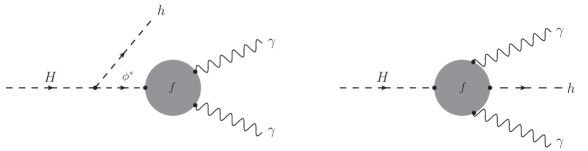
Figure 1: Group $G_{1}$-All one-loop Feynman diagrams include triangles having pole $\phi^{*}\equiv h^{*},H^{*}$ (left) and boxes (right) with exchanging fermions $f$ in loop contributing to the processes.

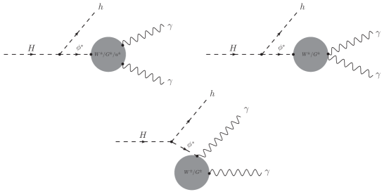
Figure 2: In the group $G_{2}\leavevmode\nobreak\ (A)$, we consider all one-loop Feynman diagrams including triangle diagrams possessing the poles of $\phi^{*}\equiv h^{*},H^{*}$ contributing to the processes.

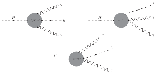
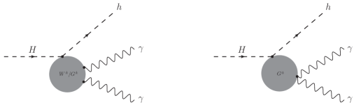
Figure 3: In the group $G_{2}\leavevmode\nobreak\ (B)$, we consider all one-loop box diagrams with exchanging $W^{\pm}$ boson, Goldstone boson $G^{\pm}$ and ghosts $u^{\pm}$ in loop contributing to the processes.

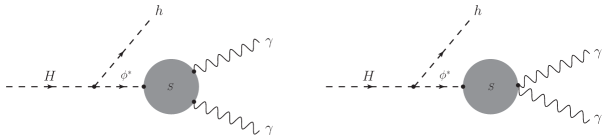
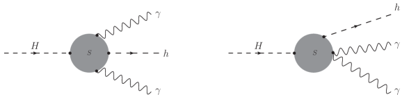
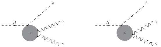
Figure 4: Group $G_{3}$-All one-loop Feynman diagrams having triangle diagrams with the poles $\phi^{*}\equiv h^{*},H^{*}$ and box diagrams by exchanging charged scalar boson $S\equiv H^{\pm}$ in loop contributing to the processes.

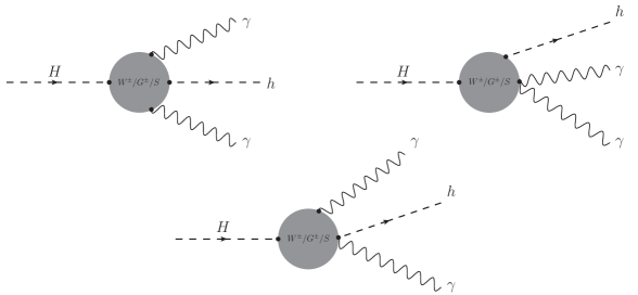
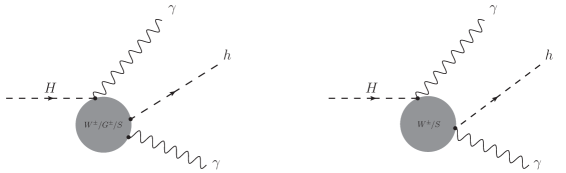
Figure 5: Group $G_{4}$- All one-loop Feynman diagrams include box diagrams with exchanging $W^{\pm}$ boson, Goldstone boson $G^{\pm}$ and charged scalar boson $S\equiv H^{\pm}$ mixing in loop contributing to processes.

In general, one-loop amplitude for $H(p)\rightarrow h(q_{1})\gamma_{\mu}(q_{2})\gamma_{\nu}(q_{3})$ is expressed in terms of Lorentz structure as follows:

$$\mathcal{A}_{H\rightarrow h\gamma\gamma} = \Big{[}F_{00}g^{\mu\nu}+F_{11}q_{1}^{\mu}q_{1}^{\nu}+F_{12}q_{1}^{\mu}q_{2}^{\nu}+F_{13}q_{3}^{\mu}q_{1}^{\nu}+F_{23}q_{3}^{\mu}q_{2}^{\nu}\Big{]}\varepsilon^{*}_{\mu}(q_{2})\varepsilon^{*}_{\nu}(q_{3}).$$ (17)

All one-loop factors are expressed as functions of the following kinematic invariant variables which they are given by

$$q_{12} = (q_{1}+q_{2})^{2}=M_{h}^{2}+2q_{1}\cdot q_{2},$$ (18)

$$q_{13} = (q_{1}+q_{3})^{2}=M_{h}^{2}+2q_{1}\cdot q_{3},$$ (19)

$$q_{23} = (q_{2}+q_{3})^{2}=2q_{2}\cdot q_{3}.$$ (20)

The kinematic invariants mentioned obey the following relation

$$q_{12}+q_{13}+q_{23}=M_{H}^{2}+M_{h}^{2}.$$ (21)

With on-shell photons in final states, the amplitude follows the so-called ward identity. As a result, in the processes we derive the following relations as:

$$F_{13} = -\frac{q_{12}-M_{h}^{2}}{q_{23}}F_{11},$$ (22)

$$F_{00} = -\frac{q_{12}-M_{h}^{2}}{2}F_{12}-\frac{q_{23}}{2}F_{23},$$ (23)

$$F_{12} = -\frac{q_{13}-M_{h}^{2}}{q_{23}}F_{11},$$ (24)

$$F_{00} = -\frac{q_{13}-M_{h}^{2}}{2}F_{13}-\frac{q_{23}}{2}F_{23},$$ (25)

Using the above relations, the amplitude can presented via two independent one-loop factors, e.g. taking $F_{11}$ and $F_{23}$ as example. In detail, the amplitude can be expressed as follows:

$$\mathcal{A}_{H\rightarrow h\gamma\gamma} = \Bigg{\{}\Bigg{[}\frac{(q_{12}-M_{h}^{2})(q_{13}-M_{h}^{2})}{2q_{23}}\cdot g^{\mu\nu}+q_{1}^{\mu}q_{1}^{\nu}+\frac{(M_{h}^{2}-q_{13})}{q_{23}}\cdot q_{1}^{\mu}q_{2}^{\nu}$$

$$+\frac{(M_{h}^{2}-q_{12})}{q_{23}}\cdot q_{3}^{\mu}q_{1}^{\nu}\Bigg{]}\cdot F_{11}+\Big{[}q_{3}^{\mu}q_{2}^{\nu}-\frac{q_{23}}{2}\cdot g^{\mu\nu}\Big{]}\cdot F_{23}\Bigg{\}}\,\varepsilon^{*}_{\mu}(q_{2})\varepsilon^{*}_{\nu}(q_{3}).$$

In this paper, we will collect two independent one-loop form factors $F_{11}$, $F_{23}$ in Eq. (3). They are expressed in terms of the scalar Passarino-Veltman (PV) one-loop integrals in following the notations of the package LoopTools and the library Collider [96]. Consequently, the decay rates and its distributions can be evaluated numerically by using one of the above-mentioned packages. We emphasize that all phenomenological results presented in the following sections are generated by using the package Collider.

The form factors are divided into triangle and box ones which are corresponding to the contributions from one-loop triangle and one-loop box diagrams. They are computed as follows:

$$F_{ab} = F_{ab}^{\textrm{Trig}}+F_{ab}^{\textrm{Box}}$$ (27)

for $ab=\{11,23\}$. The form factors $F_{ab}^{\textrm{Trig}}$ are first collected. They are calculated from all one-loop triangle Feynman diagrams. We take into account all one-loop three-point diagrams in above groups which are classified via the internal particles exchanging in the loop. In this case, off-shell of CP-even Higgses $h^{*},H^{*}$ decay into di-photon at one-loop are involved. The form factors $F_{ab}^{\textrm{Trig}}$ are contributed from fermion, $W$ boson and charged Higgses propagating in the loop. It is easy to confirm that one-loop form factors $F_{11}^{\textrm{Trig}}$ are absent in these groups. Another one-loop form factors $F_{23}^{\textrm{Trig}}$ are taken the form of:

$$F_{23}^{\textrm{Trig}} = \sum\limits_{\phi=h^{*},H^{*}}\frac{g_{Hh\,\phi}}{\Big{[}q_{23}-M_{\phi}^{2}+i\Gamma_{\phi}M_{\phi}\Big{]}}\times\left\{F_{23,f}^{\textrm{Trig}}+F_{23,W}^{\textrm{Trig}}+F_{23,H^{\pm}}^{\textrm{Trig}}\right\}.$$ (28)

Here $N^{C}_{f}$ ($Q_{f}$) is number of color (charged) for fermion $f$, respectively. All the coefficients factors $F_{23,f/W/H^{\pm}}^{\textrm{Trig}}$ are presented in terms of the scalar PV-functions in appendix Appendix C: Form factors for $H\rightarrow h\gamma\gamma$ in THDM.

By expanding PV-functions, we arrive at the final results for $F_{23}^{\textrm{Trig}}$ as follows:

$$F_{23}^{\textrm{Trig}} = \dfrac{\alpha}{4\pi}\sum\limits_{\phi=h^{*},H^{*}}\dfrac{g_{Hh\,\phi}}{\Big{[}q_{23}-M_{\phi}^{2}+i\Gamma_{\phi}M_{\phi}\Big{]}}\times$$ (29)

$$\times\Bigg{\{}\sum\limits_{f}(N^{C}_{f}Q_{f}^{2})\cdot g_{\phi ff}\cdot(4\lambda_{f})\Big{[}1+\big{(}1-\lambda_{f}\big{)}f(\lambda_{f})\Big{]}$$

$$+\dfrac{g_{\phi\,WW}}{M_{W}^{2}}\cdot\Big{[}2\rho_{\phi}+3\lambda_{W}+\lambda_{W}\big{(}8-2\rho_{\phi}-3\lambda_{W}\big{)}f(\lambda_{W})\Big{]}$$

$$-\left(\dfrac{4\;g_{\phi H^{\pm}H^{\mp}}}{q_{23}}\right)\cdot\Big{[}1-\lambda_{H^{\pm}}f(\lambda_{H^{\pm}})\Big{]}\Bigg{\}}.$$

In all above equations, we have used the variables like $\rho_{\phi}=M_{\phi}^{2}/q_{23}$ and $\lambda_{i}=4m_{i}^{2}/q_{23}$ with $m_{i}$ being $m_{f},M_{W},M_{H^{\pm}}$ in this case.

We next collect one-loop form factors $F_{ab}^{\textrm{Box}}$ which are attributed from all one-loop box diagrams appear in the above groups. The factors can be separated as follows:

$$F_{ab}^{\textrm{Box}} = -\dfrac{e^{2}}{2\pi^{2}}\sum\limits_{f}(N^{C}_{f}\;m_{f}^{2}\;Q_{f}^{2})\cdot g_{hff}\cdot g_{Hff}\times F_{ab,f}^{\textrm{Box}}$$ (30)

$$+\left(\dfrac{e^{2}}{8\pi^{2}}\right)\cdot g_{hWW}\cdot g_{HWW}\times F_{ab,W}^{\textrm{Box}}$$

$$-\left(\dfrac{e^{2}}{8\pi^{2}M_{W}^{2}}\right)\cdot g_{hH^{\pm}W^{\mp}}\cdot g_{HH^{\pm}W^{\mp}}\times F_{ab,WH^{\pm}}^{\textrm{Box}}$$

$$+\left(\dfrac{e^{2}}{4\pi^{2}}\right)\times F_{ab,H^{\pm}}^{\textrm{Box}}$$

for $ab=\{11,23\}$. All one-loop form factors artributing in Eq. (30), $F_{ab,f/W/WH^{\pm}/H^{\pm}}^{\textrm{Box}}$ are presented in detail in the appendix Appendix C: Form factors for $H\rightarrow h\gamma\gamma$ in THDM.

After collecting the one-loop form factors, we perform the numerical checks for the calculation. We verify that all factors are ultraviolet (UV) and infrared (IR) finiteness. Furthermore, due to the on-shell photon in final state, the amplitude for the decay channel also follows the so-called ward identity. The identity is also confirmed numerically in this work. One finds the results are good stability. The numerical test are presented in the next section. Having all correctness one-loop form factors, the decay rates are then evaluated as follows:

$$\Gamma_{H\rightarrow h\gamma\gamma} = \dfrac{1}{256\pi^{3}M_{H}^{3}}\int\limits_{q_{23}^{\text{min}}}^{q_{23}^{\text{max}}}dq_{23}\int\limits_{q_{13}^{\text{min}}}^{q_{13}^{\text{max}}}dq_{13}\,\sum\limits_{\text{pol.}}\big{|}\mathcal{A}_{H\rightarrow h\gamma\gamma}\big{|}^{2}$$ (31)

where total amplitude is squared as

$$\sum\limits_{\text{pol.}}\big{|}\mathcal{A}_{H\rightarrow h\gamma\gamma}\big{|}^{2} = \dfrac{1}{2}\Bigg{\{}\Bigg{[}\dfrac{\big{(}M_{h}^{2}-q_{13}\big{)}\big{(}M_{H}^{2}-q_{13}\big{)}}{q_{23}^{2}}\Big{(}2\;q_{23}\cdot q_{13}+[M_{h}^{2}-q_{13}][M_{H}^{2}-q_{13}]\Big{)}$$

$$\hskip 14.22636pt+\big{(}q_{13}^{2}+M_{h}^{4}\big{)}\Bigg{]}\big{|}F_{11}\big{|}^{2}-2q_{23}\;M_{h}^{2}\;\mathcal{R}e\Big{[}F_{11}\times F_{23}^{*}\Big{]}+q_{23}^{2}\big{|}F_{23}\big{|}^{2}\Bigg{\}}.$$

The limitations of integrand are generally expressed for the decay process as follows:

$$q_{23}^{\text{min}} = 0,$$ (33)

$$q_{23}^{\text{max}} = (M_{H}-M_{h})^{2},$$ (34)

$$q_{13}^{\text{max(min)}} = \dfrac{1}{2}\Big{\{}M_{H}^{2}+M_{h}^{2}-q_{23}\pm\Big{[}\big{(}M_{H}^{2}+M_{h}^{2}-q_{23}\big{)}^{2}-4M_{H}^{2}M_{h}^{2}\Big{]}^{1/2}\Big{\}}.$$ (35)

4 Phenomenological results

We turn our attention to discuss the phenomenological results for the CP-even Higgs decay process $H\rightarrow h\gamma\gamma$ in THDM. As usual, before arriving the phenomenological studies in concrete, we first summary the current limitations for the parameter space of THDM. Considering theoretical and experimental constraints for THDM, we find the current regions for the parameter space in this model. From theoretical side, the constraints reply on the topics like the requirements of perturbative regime, tree-level unitarity of the theories and vacuum stability conditions for the scalar Higgs potential. These theoretical constraints have reported in the following Refs. [69, 70, 71, 72, 74] and references therein. In the aspect of the experimental constraints, we take into consideration the electroweak precision tests (EWPT) for THDM which the subjects have implicated at LEP [75, 76]. Furthermore, the direct and indirect searches for the masses of scalar particles for THDM have performed at the LEP, the Tevaron and the LHC as summarized in the Ref. [73]. In addition, implicating for one-loop induced decays of $h\rightarrow\gamma\gamma$ and $h\rightarrow Z\gamma$ in THDM have performed in Refs. [45, 46] and references therein. Combining all the above constraints, we can take logically the parameter space for our analysis in THDM as follows. We select $126$ GeV $\leq M_{H}\leq 1000$ GeV, $60$ GeV $\leq M_{A^{0}}\leq 1000$ GeV and $80$ GeV $\leq M_{H^{\pm}}\leq 1000$ GeV in the type I and type X of THDM. For the Type-II and Y, we can scan consistently the physical parameters as follows: $500$ GeV $\leq M_{H}\leq 1000$ GeV, $500$ GeV $\leq M_{A^{0}}\leq 1000$ GeV and $580$ GeV $\leq M_{H^{\pm}}\leq 1500$ GeV. In both types, one takes $2\leq t_{\beta}\leq 20$, $0.95\leq s_{\beta-\alpha}\leq 1$ for the alignment limit of the SM (we take $s_{\beta-\alpha}=0.98$ for all below physical results) and can be taken the $Z_{2}$ breaking parameter as $m_{12}^{2}=M_{H}^{2}s_{\beta}c_{\beta}$. Last but not least, from flavor experimental data, the further limitations on $t_{\beta}$, $M_{H^{\pm}}$ have also performed for the THDM with the softly broken $Z_{2}$ symmetry in Ref. [98]. Following the results in Ref. [98], we find that the small values of $t_{\beta}$ are favoured for matching the flavor experimental data. To complete our discussions, we are also interested in considering the small values of $t_{\beta}$ (scan it reasonably over the region of $2\leq t_{\beta}\leq 10$ in some cases, for examples) in our work. In our analysis, the decay widths of SM-like Higgs is taken from experimental value (as indicated in below).

Secondly, other input parameters in this work are used as follows. For gauge bosons, we take $M_{Z}=91.1876$ GeV, $\Gamma_{Z}=2.4952$ GeV, $M_{W}=80.379$ GeV, $\Gamma_{W}=2.085$ GeV. For SM-like Higgs boson, we use $M_{h^{0}}=125.1$ GeV, $\Gamma_{h^{0}}=4.07\cdot 10^{-3}$ GeV. The masses of all fermions are applied as $m_{e}=0.00052$ GeV, $m_{\mu}=0.10566$ GeV and $m_{\tau}=1.77686$ GeV. In the quark sector, their masses are taken as $m_{u}=0.00216$ GeV, $m_{d}=0.0048$ GeV, $m_{c}=1.27$ GeV, $m_{s}=0.93$ GeV, $m_{t}=173.0$ GeV, and $m_{b}=4.18$ GeV. In the $G_{\mu}$-scheme, the Fermi constant is considered as an input parameter, $G_{\mu}=1.16638\cdot 10^{-5}$ GeV^-2 is taken. The electroweak constant is then obtained subsequently:

$$\alpha=\sqrt{2}/\pi G_{\mu}M_{W}^{2}(1-M_{W}^{2}/M_{Z}^{2})=1/132.184.$$ (36)

Lastly, we apply the further cut as follows $q_{23}^{\textrm{min}}=4\left(E_{\gamma}^{\textrm{cut}}\right)^{2}=100\;\textrm{GeV}^{2}$. For all numerical results presented in the following subsection, we take $s_{\beta-\alpha}=0.98$ for the alignment THDM limit.

4.1 Numerical checks: the $UV$, $IR$-finiteness, the ward identity

We first present the numerical checks for all one-loop form factors. The factors are ultraviolet (UV) and infrared (IR) finiteness. In Tables 4,  5 (Tables 6,  7), we show the numerical checks for the factor $F_{23}$ ($F_{11}$), respectively. In these Tables of data, we select the input parameters as follows: $M_{H}=500\,\text{GeV},M_{H^{\pm}}=200\,\text{GeV},q_{23}=100^{2}\,\text{GeV}^{2},q_{13}=-50^{2}\,\text{GeV}^{2}$ and $s_{\beta-\alpha}=0.98,t_{\beta}=5$ for an example. In Table 4 (in Table 5), we show correspondingly to the numerical results for $F_{23}$ for the case of $M^{2}=+150^{2}$ GeV² (for $M^{2}=-150^{2}$ GeV²).

Diagrams / $\big{(}C_{UV},\lambda^{2}\big{)}$	$\big{(}0,1\big{)}$	$\big{(}10^{2},10^{4}\big{)}$
$h^{*}$-pole in Fig. 2	$+1.329047959903308\cdot 10^{-7}$	$+1.329047959903318\cdot 10^{-7}$
$H^{*}$-pole in Fig. 2	$-5.051869605168205\cdot 10^{-11}$	$-5.051869605168235\cdot 10^{-11}$
Fig. 3	$+5.064470955527445\cdot 10^{-9}$	$+5.064470955527416\cdot 10^{-9}$
	$+1.167619118910286\cdot 10^{-8}\,i$	$+1.167619118910286\cdot 10^{-8}\,i$
Fig. 5	$+1.183638848868308\cdot 10^{-9}$	$+1.183638848868356\cdot 10^{-9}$
	$-1.988356571739141\cdot 10^{-9}\,i$	$-1.988356571739141\cdot 10^{-9}\,i$
Sum	$+1.391023870986748\cdot 10^{-7}$	$+1.391023870986743\cdot 10^{-7}$
	$+9.68783461736372\cdot 10^{-9}\,i$	$+9.68783461736372\cdot 10^{-9}\,i$

Table 4: Numerical checks for form factor $F_{23}$ for the case of $M^{2}=+150^{2}$ GeV².

Diagrams / $\big{(}C_{UV},\lambda^{2}\big{)}$	$\big{(}0,1\big{)}$	$\big{(}10^{2},10^{4}\big{)}$
$h^{*}$-pole in Fig. 2	$-8.85535379601663\cdot 10^{-8}$	$-8.85535379601666\cdot 10^{-8}$
$H^{*}$-pole in Fig. 2	$+1.013995093472795\cdot 10^{-10}$	$+1.013995093472791\cdot 10^{-10}$
Fig. 3	$-6.424613246657161\cdot 10^{-9}$	$-6.424613246657169\cdot 10^{-9}$
	$+1.167619118910286\cdot 10^{-8}\,i$	$+1.167619118910286\cdot 10^{-8}\,i$
Fig. 5	$+1.183638848868308\cdot 10^{-9}$	$+1.183638848868306\cdot 10^{-9}$
	$-1.988356571739141\cdot 10^{-9}\,i$	$-1.988356571739141\cdot 10^{-9}\,i$
Sum	$-9.36931128488564\cdot 10^{-8}$	$-9.36931128488565\cdot 10^{-8}$
	$+9.68783461736372\cdot 10^{-9}\,i$	$+9.68783461736372\cdot 10^{-9}\,i$

Table 5: Numerical checks for form factor $F_{23}$ for the case of $M^{2}=-150^{2}\,\text{GeV}^{2}$.

Numerical checks for $F_{11}$ are shown in the following Tables 6 (for $M^{2}=+150^{2}$ GeV²), 7 (for $M^{2}=-150^{2}\,\text{GeV}^{2}$), respectively. The data shows that numerical results are good stability when we varying $C_{UV},\mu^{2}$ parameters. It indicates that the factors $F_{23}$ and $F_{11}$ are $UV$, $IR$-finiteness.

Diagrams / $\big{(}C_{UV},\lambda^{2}\big{)}$	$\big{(}0,1\big{)}$	$\big{(}10^{2},10^{4}\big{)}$
$h^{*}$-pole in Fig. 2	$-$	$-$
$H^{*}$-pole in Fig. 2	$-$	$-$
Fig. 3	$-4.40424746463004\cdot 10^{-9}$	$-4.40424746463005\cdot 10^{-9}$
	$+3.94576208393711\cdot 10^{-9}\,i$	$+3.94576208393711\cdot 10^{-9}\,i$
Fig. 5	$+2.679331531268657\cdot 10^{-9}$	$+2.679331531268655\cdot 10^{-9}$
	$-5.476182469709093\cdot 10^{-9}\,i$	$-5.476182469709093\cdot 10^{-9}\,i$
Sum	$-1.724915933361384\cdot 10^{-9}$	$-1.724915933361380\cdot 10^{-9}$
	$-1.530420385771982\cdot 10^{-9}\,i$	$-1.530420385771982\cdot 10^{-9}\,i$

Table 6: Numerical checks for form factor $F_{11}$ for the case of $M^{2}=+150^{2}\,\text{GeV}^{2}$.

Diagrams / $\big{(}C_{UV},\lambda^{2}\big{)}$	$\big{(}0,1\big{)}$	$\big{(}10^{2},10^{4}\big{)}$
$h^{*}$-pole in Fig. 2	$-$	$-$
$H^{*}$-pole in Fig. 2	$-$	$-$
Fig. 3	$-4.40424746463004\cdot 10^{-9}$	$-4.40424746463005\cdot 10^{-9}$
	$+3.94576208393711\cdot 10^{-9}\,i$	$+3.94576208393711\cdot 10^{-9}\,i$
Fig. 5	$+2.679331531268657\cdot 10^{-9}$	$+2.679331531268655\cdot 10^{-9}$
	$-5.476182469709093\cdot 10^{-9}\,i$	$-5.476182469709093\cdot 10^{-9}\,i$
Sum	$-1.724915933361384\cdot 10^{-9}$	$-1.724915933361380\cdot 10^{-9}$
	$-1.530420385771982\cdot 10^{-9}\,i$	$-1.530420385771982\cdot 10^{-9}\,i$

Table 7: Numerical checks for form factor $F_{11}$ for the case of $M^{2}=-150^{2}\,\text{GeV}^{2}$.

Furthermore, due to the on-shell photons in final state, the amplitude for the decay channels also obey the so-called ward identity. In concrete, we confirm numerically the following identity

$$F_{00} = F_{T}=\dfrac{(q_{12}-M_{h}^{2})(q_{13}-M_{h}^{2})}{2q_{23}}F_{11}-\dfrac{q_{23}}{2}F_{23}.$$ (37)

To arrive this relation, we have already replaced $F_{13}$ by $F_{11}$ in Eq. 22. In this work, the factors $F_{00}$ and $F_{11},F_{23}$ are collected independent. All of them are presented in terms of the scalar PV functions. We then verify numerically the identity in Eq. (37). The results of this test are shown in Tables 8, 9. We note that all relations in Eqs. 22, 23, 24, 25 are verified numerically. But we show only the numerical results for Eq. (37) as a typical example. Moreover, it is stress that we present only analytical expressions for $F_{11},F_{23}$ taking into account the decay rates in the current paper. All physical results are then generated via the factors $F_{11},F_{23}$. From the data, we find that the results are good stability and confirm the identity in Eq. (37).

	$F_{11}$	$-$
$\big{(}q_{13},q_{23},M^{2}\big{)}$	$F_{23}$	$-$
	$F_{T}$	$F_{00}$
	$-1.524721445905201\cdot 10^{-7}$	$-$
	$-7.110585958979337\cdot 10^{-8}\,i$
$\big{(}+150^{2},+250^{2},+150^{2}\big{)}$	$+3.651043549471353\cdot 10^{-7}$	$-$
	$-3.437209227618915\cdot 10^{-7}\,i$
	$-0.01278816221085315$	$-0.01278816221085316$
	$+0.01009834059249554\,i$	$+0.01009834059249555\,i$
	$-8.89913100855076\cdot 10^{-8}$	$-$
	$-6.375931724486408\cdot 10^{-8}\,i$
$\big{(}-150^{2},+250^{2},+150^{2}\big{)}$	$+2.775629657896212\cdot 10^{-7}$	$-$
	$-2.777884080549074\cdot 10^{-7}\,i$
	$-0.002970210139871302$	$-0.002970210139871301$
	$+0.01276735098373022\,i$	$+0.01276735098373023\,i$
	$+8.14172209386663\cdot 10^{-8}$	$-$
	$+3.110963119073888\cdot 10^{-8}\,i$
$\big{(}+150^{2},-250^{2},+150^{2}\big{)}$	$+1.766382780308712\cdot 10^{-7}$	$-$
	$-1.386843033642122\cdot 10^{-7}\,i$
	$+0.004226065602186965$	$+0.004226065602186968$
	$-0.004828278017271411\,i$	$-0.004828278017271414\,i$
	$+4.98006304470054\cdot 10^{-8}$	$-$
	$+2.575736201977261\cdot 10^{-8}\,i$
$\big{(}-150^{2},-250^{2},+150^{2}\big{)}$	$+1.453614520978374\cdot 10^{-7}$	$-$
	$-1.309372710452731\cdot 10^{-7}\,i$
	$+0.00963426277087704$	$+0.00963426277087701$
	$-0.001458304822241892\,i$	$-0.001458304822241893\,i$

Table 8: ward identity check $F_{T}=F_{00}$ for the case of $M^{2}=+150^{2}$ GeV².

	$F_{11}$	$-$
$\big{(}q_{13},q_{23},M^{2}\big{)}$	$F_{23}$	$-$
	$F_{T}$	$F_{00}$
	$-3.164637261836014\cdot 10^{-7}$
	$-1.446908683148855\cdot 10^{-7}\,i$	$-$
$\big{(}+150^{2},+250^{2},-150^{2}\big{)}$	$+9.06539595717883\cdot 10^{-7}$
	$-7.511627252884878\cdot 10^{-7}\,i$	$-$
	$-0.03119082320101478$	$-0.03119082320101476$
	$+0.02216554224388151\,i$	$+0.02216554224388154\,i$
	$-1.932366818004465\cdot 10^{-7}$
	$-1.323298998771165\cdot 10^{-7}\,i$	$-$
$\big{(}-150^{2},+250^{2},-150^{2}\big{)}$	$+6.979798741398192\cdot 10^{-7}$
	$-5.980635610637261\cdot 10^{-7}\,i$	$-$
	$-0.00942694241053888$	$-0.00942694241053889$
	$+0.0271707764493079\,i$	$+0.0271707764493075\,i$
	$+1.502250124801403\cdot 10^{-7}$
	$+7.086353703138775\cdot 10^{-8}\,i$	$-$
$\big{(}+150^{2},-250^{2},-150^{2}\big{)}$	$+3.880760921445276\cdot 10^{-7}$
	$-3.197203563280603\cdot 10^{-7}\,i$	$-$
	$+0.00974000546640239$	$+0.00974000546640232$
	$-0.01111742282172064\,i$	$-0.01111742282172063\,i$
	$+1.011443268310633\cdot 10^{-7}$
	$+5.619181764807639\cdot 10^{-8}\,i$	$-$
$\big{(}-150^{2},-250^{2},-150^{2}\big{)}$	$+3.072281617154063\cdot 10^{-7}$
	$-2.933174559185206\cdot 10^{-7}\,i$	$-$
	$+0.01994208102813598$	$+0.01994208102813591$
	$-0.003421005171538428\,i$	$-0.003421005171538422\,i$

Table 9: ward identity check $F_{T}=F_{00}$ for $M^{2}=-150^{2}$ GeV².

4.2 Phenomenological analyses

We are interested in the differential decay rates of $H\rightarrow h\gamma\gamma$ with respect to the invariant mass of two photons $m_{\gamma\gamma}$, are presented as functions of of $M_{H^{\pm}}$ and $t_{\beta}$. In fact, we are concerned the distributions which are defined as follows:

$$\mathcal{R}_{\gamma\gamma}(M_{H},M_{H^{\pm}},t_{\beta})=\frac{1}{\Gamma_{H\rightarrow\gamma\gamma}}\frac{\Gamma_{H\rightarrow h\gamma\gamma}}{dm_{\gamma\gamma}}.$$ (38)

In this formula, $\Gamma_{H\rightarrow\gamma\gamma}$ is obtained by using the form factors in Eq. 64.

In Fig. 6, we show $\mathcal{R}_{\gamma\gamma}$ for the case of $M_{H}=200$ GeV at $t_{\beta}=2$ (left), $t_{\beta}=8$ (right). In the plots, the rectangle points connecting with red line are shown for the data of $\mathcal{R}_{\gamma\gamma}$ at $M_{H^{\pm}}=100$ GeV. The triangle points with green line are presented for $\mathcal{R}_{\gamma\gamma}$ at $M_{H^{\pm}}=500$ GeV. While the circle points with blue line are for $\mathcal{R}_{\gamma\gamma}$ at $M_{H^{\pm}}=1000$ GeV. We find that the decay rates of $\Gamma_{H\rightarrow h\gamma\gamma}$ develop with $m_{\gamma\gamma}$ in this case. In general, decay rates are proportional to $1/t_{\beta}$ and charged Higgs mass $M_{H^{\pm}}$. At high mass region of $m_{\gamma\gamma}$, the decay rates are more dependent on the charged Higgs masses $M_{H^{\pm}}$. It is also interested to observe that the decay rates being unchanged when $M_{H^{\pm}}$ are larged. It means that the contributions of charged Higgs to these processes tend to constant values at higher-mass region of charged Higgs.

$\frac{1}{\Gamma_{H\rightarrow\gamma\gamma}}\frac{\Gamma_{H\rightarrow h\gamma\gamma}}{dm_{\gamma\gamma}}$	$\frac{1}{\Gamma_{H\rightarrow\gamma\gamma}}\frac{\Gamma_{H\rightarrow h\gamma\gamma}}{dm_{\gamma\gamma}}$
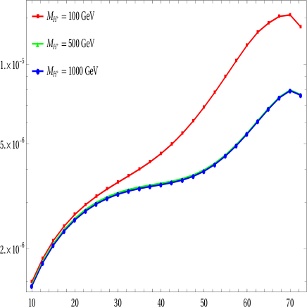
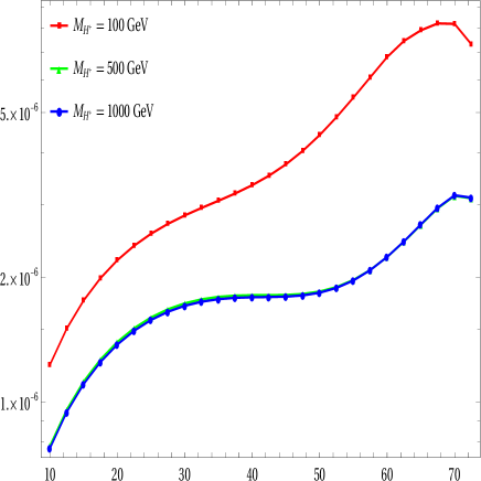
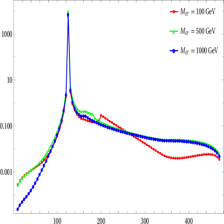
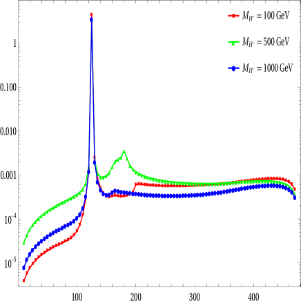
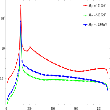
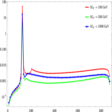
$m_{\gamma\gamma}$ [GeV]	$m_{\gamma\gamma}$ [GeV]

Figure 6: The values of $\mathcal{R}_{\gamma\gamma}$ for the case of $M_{H}=200$ GeV at $t_{\beta}=2$ (left), $t_{\beta}=8$ (right). In the plots, the rectangle points with red line are shown for $\mathcal{R}_{\gamma\gamma}$ at $M_{H^{\pm}}=100$ GeV. The triangle points with green line are presented for $\mathcal{R}_{\gamma\gamma}$ at $M_{H^{\pm}}=500$ GeV. While the circle points with blue line are for $\mathcal{R}_{\gamma\gamma}$ at $M_{H^{\pm}}=1000$ GeV.

In Fig. 7, we show for the values of $\mathcal{R}_{\gamma\gamma}$ at $M_{H}=600$ GeV with $t_{\beta}=2$ (left), $t_{\beta}=8$ (right). We use the same previous notations for all lines of data which are indicated for the values of $\mathcal{R}_{\gamma\gamma}$ corresponding to the charged Higgs mass $M_{H^{\pm}}$ in these Figures. One finds a peak of $m_{\gamma\gamma}=M_{h}=125$ GeV in both cases of $t_{\beta}$. In general, the decay rates develop to the peak and decrease rapidly beyond the peak. Overall, the decay rates depend on $1/t_{\beta}$. Unlike the previous case, in the higher-mass regions of $M_{H}$, the dependence of decay rates on $M_{H^{\pm}}$ is more complicated.

$\frac{1}{\Gamma_{H\rightarrow\gamma\gamma}}\frac{\Gamma_{H\rightarrow h\gamma\gamma}}{dm_{\gamma\gamma}}$	$\frac{1}{\Gamma_{H\rightarrow\gamma\gamma}}\frac{\Gamma_{H\rightarrow h\gamma\gamma}}{dm_{\gamma\gamma}}$
$m_{\gamma\gamma}$ [GeV]	$m_{\gamma\gamma}$ [GeV]

Figure 7: The values of $\mathcal{R}_{\gamma\gamma}$ for the case of $M_{H}=600$ GeV at $t_{\beta}=2$ (left), $t_{\beta}=8$ (right). In the plots, the rectangle points with red line are shown for $\mathcal{R}_{\gamma\gamma}$ at $M_{H^{\pm}}=100$ GeV. The triangle points with green line are presented for $\mathcal{R}_{\gamma\gamma}$ at $M_{H^{\pm}}=500$ GeV. While the circle points with blue line are for $\mathcal{R}_{\gamma\gamma}$ at $M_{H^{\pm}}=1000$ GeV.

In the next case, we consider the values of $\mathcal{R}_{\gamma\gamma}$ as functions of the invariant mass of two external photons, charged Higgs masses, and $t_{\beta}$, as shown in Fig. 8. The distributions are generated at $t_{\beta}=2$ (left), $t_{\beta}=8$ (right). We also use the same notation for the lines which are shown the values of $\mathcal{R}_{\gamma\gamma}$ corresponding to the charged Higgs masses in the plots. In all cases, one finds a peak of $m_{\gamma\gamma}=M_{h}=125$ GeV. The decay rates develop to the peak and decrease rapidly beyond the peak. In general, the decay rates depend on $1/t_{\beta}$. As same previous cases, we find that the dependence of decay rates on $M_{H^{\pm}}$ is more complicated in the higher-mass regions of $M_{H}$.

$\frac{1}{\Gamma_{H\rightarrow\gamma\gamma}}\frac{\Gamma_{H\rightarrow h\gamma\gamma}}{dm_{\gamma\gamma}}$	$\frac{1}{\Gamma_{H\rightarrow\gamma\gamma}}\frac{\Gamma_{H\rightarrow h\gamma\gamma}}{dm_{\gamma\gamma}}$
$m_{\gamma\gamma}$ [GeV]	$m_{\gamma\gamma}$ [GeV]

Figure 8: The values of $\mathcal{R}_{\gamma\gamma}$ for the case of $M_{H}=1000$ GeV at $t_{\beta}=2$ (left), $t_{\beta}=8$ (right). In the plots, the rectangle points with red line are shown for $\mathcal{R}_{\gamma\gamma}$ at $M_{H^{\pm}}=100$ GeV. The triangle points with green line are presented for $\mathcal{R}_{\gamma\gamma}$ at $M_{H^{\pm}}=500$ GeV. While the circle points with blue line are for $\mathcal{R}_{\gamma\gamma}$ at $M_{H^{\pm}}=1000$ GeV.

Since, the current paper focuses mainly on the analytic structure as well as test for the ward identity of the processes. Detailed phenomenological results for the processes which we study correlations between decay rates of $H\rightarrow h\gamma\gamma$ and $H\rightarrow\gamma\gamma$, $h\rightarrow\gamma\gamma$, will be discussed in more concrete. Furthermore, the implications for the processes with combining the updated experimental data at the colliders should be examined in further detail. These topics are far from the scope of the paper. We plan to address the mentioned topics in our future publications.

5 Conclusions

We have presented the first analytical results for one-loop induced contributions to the important decay channels of CP-even Higgs $H\rightarrow\gamma\gamma$ and $H\rightarrow h\gamma\gamma$ with $h$ being standard model-like Higgs boson within the framework of Two Higgs Doublet Model. Analytical expressions for one-loop form factors are written in terms of the basis PV-functions following the standard notations of the package LoopTools and the library Collider. Subsequently, physical results can be evaluated numerically by using one of the mentioned packages. Analytical formulas shown in this paper, have verified by the numerical checks such as the UV and IR-finiteness of one-loop amplitude. Furthermore, due to on-shell photons in final states, the corresponding one-loop amplitude obeys the so-called ward identity. The identity has also tested numerically. We found that numerical results for the tests are good stability. In phenomenological studies, the differential decay rates as functions of the invariant of two photons in final state of $H\rightarrow h\gamma\gamma$ are first studied in parameter space for all types of Two Higgs Doublet Models.

Acknowledgment:  This research is funded by Vietnam National Foundation for Science and Technology Development (NAFOSTED) under the grant number $103.01$-$2023.16$. Khiem Hong Phan and Dzung Tri Tran express their gratitude to all the valuable support from Duy Tan University, for the 30th anniversary of establishment (Nov. 11, 1994 - Nov. 11, 2024) towards "Integral, Sustainable and Stable Development".

Appendix A: Tensor reduction for one-loop integrals

In this work, we follow tensor reduction method developed in Ref. [99]. The method is reviewed briefly in this appendix. In general, tensor one-loop integrals with $N$-external lines can be decomposed into the basis integrals such as scalar one-loop one-, two-, three- and four- point integrals (they are noted hereafter as $A_{0},B_{0},C_{0}$ and $D_{0}$), respectively. The definition for tensor one-loop integrals with rank $P$ are as follows:

$$\{A;B;C;D\}^{\mu_{1}\mu_{2}\cdots\mu_{P}}=(\mu^{2})^{2-d/2}\int\frac{d^{d}k}{(2\pi)^{d}}\dfrac{k^{\mu_{1}}k^{\mu_{2}}\cdots k^{\mu_{P}}}{\{D_{1};D_{1}D_{2};D_{1}D_{2}D_{3};D_{1}D_{2}D_{3}D_{4}\}}.$$ (39)

Where the numerator is expressed in terms of the Lorentz structure of the corresponding tensor one-loop integrals with rank $P$. While $D_{j}$ ($j=1,\cdots,4$) are for the inverse Feynman propagators in the denominators. We show explicitly the Feynman propagators as follows:

$$D_{j}^{-1}=\dfrac{1}{[(k+q_{j})^{2}-m_{j}^{2}+i\rho]}.$$ (40)

In this definition, $q_{j}=\sum\limits_{i=1}^{j}p_{i}$, $p_{i}$ are the external momenta and $m_{j}$ are internal masses in the loops. Dimensional regularization for one-loop integrals are performed within the space-time dimension $d=4-2\varepsilon$ for $\varepsilon\rightarrow 0$. The parameter $\mu^{2}$ in the integrals play role of a renormalization scale. Several reduction formulas for one-loop one-, two-, three- and four-point tensor integrals up to rank $P=3$ [99] are shown explicitly, for examples,

$$A^{\mu} = 0,$$ (41)

$$A^{\mu\nu} = g^{\mu\nu}A_{00},$$ (42)

$$A^{\mu\nu\rho} = 0,$$ (43)

$$B^{\mu} = q^{\mu}B_{1},$$ (44)

$$B^{\mu\nu} = g^{\mu\nu}B_{00}+q^{\mu}q^{\nu}B_{11},$$ (45)

$$B^{\mu\nu\rho} = \{g,q\}^{\mu\nu\rho}B_{001}+q^{\mu}q^{\nu}q^{\rho}B_{111},$$ (46)

$$C^{\mu} = q_{1}^{\mu}C_{1}+q_{2}^{\mu}C_{2}=\sum\limits_{i=1}^{2}q_{i}^{\mu}C_{i},$$ (47)

$$C^{\mu\nu} = g^{\mu\nu}C_{00}+\sum\limits_{i,j=1}^{2}q_{i}^{\mu}q_{j}^{\nu}C_{ij},$$ (48)

$$C^{\mu\nu\rho} = \sum_{i=1}^{2}\{g,q_{i}\}^{\mu\nu\rho}C_{00i}+\sum_{i,j,k=1}^{2}q^{\mu}_{i}q^{\nu}_{j}q^{\rho}_{k}C_{ijk},$$ (49)

$$D^{\mu} = q_{1}^{\mu}D_{1}+q_{2}^{\mu}D_{2}+q_{3}^{\mu}D_{3}=\sum\limits_{i=1}^{3}q_{i}^{\mu}D_{i},$$ (50)

$$D^{\mu\nu} = g^{\mu\nu}D_{00}+\sum\limits_{i,j=1}^{3}q_{i}^{\mu}q_{j}^{\nu}D_{ij},$$ (51)

$$D^{\mu\nu\rho} = \sum_{i=1}^{3}\{g,q_{i}\}^{\mu\nu\rho}D_{00i}+\sum_{i,j,k=1}^{3}q^{\mu}_{i}q^{\nu}_{j}q^{\rho}_{k}D_{ijk}.$$ (52)

In these expression, we have used the notation [99] $\{g,q_{i}\}^{\mu\nu\rho}$. The tensor is defined as follows: $\{g,q_{i}\}^{\mu\nu\rho}=g^{\mu\nu}q^{\rho}_{i}+g^{\nu\rho}q^{\mu}_{i}+g^{\mu\rho}q^{\nu}_{i}$. All scalar coefficients $A_{00},B_{1},\cdots,D_{333}$ in the right hand sides of the above equations are so-called Passarino-Veltman functions (called as PV-function) [99]. The basic PV-functions are well-known and have been implemented into LoopTools [95] as well as the library Collier [96] for numerical evaluations.

In this calculation, analytic results for one-loop form factors are presented in terms of the basic PV-functions with following the short notations as:

$$\{A;B;C;D\}_{ijk\cdots}^{[f_{1},f_{2},\cdots](\cdots)}[q_{i}\cdot q_{j}]=\{A;B;C;D\}_{ijk\cdots}^{(\cdots)}[q_{i}\cdot q_{j};m_{f_{1}}^{2},m_{f_{2}}^{2},\cdots].$$ (53)

We also expand scalar one-loop three-point functions in terms of the basic $f$-function as follows:

$$C_{0}(0,0,M^{2},m^{2},m^{2},m^{2}) = -\dfrac{2}{M^{2}}f\left(\frac{4m^{2}}{M^{2}}\right).$$ (54)

Where $f$-function is defined as in [100]:

$$f(\tau) =\left\{\begin{array}[]{rcl}\arcsin^{2}\sqrt{\tau}&\mbox{for}&\tau\leq 1,\\ &\\ -\frac{1}{4}\left[\log\dfrac{1+\sqrt{1-\tau^{-1}}}{1-\sqrt{{1-\tau^{-1}}}}-i\pi\right]^{2}&\mbox{for}&\tau>1.\end{array}\right.$$ (58)

Appendix B: One-loop induced of $\phi\rightarrow\gamma\gamma$ in THDM

In this appendix, one-loop induced of $\phi(k)\rightarrow\gamma_{\mu}(k_{1})\gamma_{\nu}(k_{2})$ in THDM are shown. The CP-even Higgses $\phi$ can be the SM-like Higgs $h$ and another CP-even Higgs $H$. General one-loop amplitude for the decau channels $\phi(k)\rightarrow\gamma_{\mu}(k_{1})\gamma_{\nu}(k_{2})$ can be expressed as follows:

$$\mathcal{A}_{\phi\rightarrow\gamma\gamma} = F_{\phi\rightarrow\gamma\gamma}\cdot\Big{[}k_{2}^{\mu}k_{1}^{\nu}-\frac{k_{12}}{2}\cdot g^{\mu\nu}\Big{]}\cdot\varepsilon^{*}_{\mu}(k_{1})\varepsilon^{*}_{\nu}(k_{2}).$$ (59)

Where $k^{2}=k_{12}=(k_{1}+k_{2})^{2}=2k_{1}\cdot k_{2}=M_{\phi}^{2}$. One-loop form factors are given by

$$F_{\phi\rightarrow\gamma\gamma} = \dfrac{e^{2}}{2\pi^{2}}\sum\limits_{f}N^{C}_{f}\;Q_{f}^{2}\cdot g_{\phi ff}\times F_{\phi\rightarrow\gamma\gamma}^{f}$$ (60)

$$+\dfrac{e^{2}}{16\pi^{2}}\cdot\dfrac{g}{M_{W}}\cdot\kappa_{\phi\,WW}\times F_{\phi\rightarrow\gamma\gamma}^{W}$$

$$+\frac{e^{2}}{4\pi^{2}}\cdot\left(\dfrac{g_{\phi\,H^{\pm}H^{\mp}}}{M_{\phi}^{2}}\right)\times F_{\phi\rightarrow\gamma\gamma}^{H^{\pm}}.$$

Here we already used $g_{\phi\,WW}=\kappa_{\phi\,WW}\cdot g_{h\,WW}^{\textrm{SM}}$ for $\phi=h,H$ and $g_{h\,WW}^{\textrm{SM}}=\dfrac{2M_{W}^{2}}{v}$. In this equation, each form factor is given explicitly as follows:

$$F_{\phi\rightarrow\gamma\gamma}^{f} = \left(\frac{m_{f}^{2}}{M_{\phi}^{2}}\right)\Big{[}2-\big{(}M_{\phi}^{2}-4m_{f}^{2}\big{)}C_{0}(0,0,M_{\phi}^{2},m_{f}^{2},m_{f}^{2},m_{f}^{2})\Big{]},$$ (61)

$$F_{\phi\rightarrow\gamma\gamma}^{W} = \left(\frac{2}{M_{\phi}^{2}}\right)\Big{[}M_{\phi}^{2}+6M_{W}^{2}-6M_{W}^{2}(M_{\phi}^{2}-2M_{W}^{2})C_{0}(0,0,M_{\phi}^{2},M_{W}^{2},M_{W}^{2},M_{W}^{2})\Big{]},$$ (62)

$$F_{\phi\rightarrow\gamma\gamma}^{H^{\pm}} = -1-2M_{H^{\pm}}^{2}C_{0}(0,0,M_{\phi}^{2},M_{H^{\pm}}^{2},M_{H^{\pm}}^{2},M_{H^{\pm}}^{2}).$$ (63)

Expanding scalar one-loop three-point functions in all above equations as in Eq. (54), we the arrive at

$$F_{\phi\rightarrow\gamma\gamma} = \dfrac{\alpha}{4\pi}\Bigg{\{}\sum\limits_{f}N^{C}_{f}\,Q_{f}^{2}\cdot g_{\phi ff}\cdot(4\tau_{f})\cdot\Big{[}1+\Big{(}1-\tau_{f}\Big{)}f(\tau_{f})\Big{]}$$ (64)

$$\hskip 14.22636pt+\left(\dfrac{g_{\phi\,WW}}{M_{W}^{2}}\right)\cdot\Big{[}2+3\tau_{W}+3\tau_{W}\big{(}2-\tau_{W}\big{)}f(\tau_{W})\Big{]}$$

$$\hskip 14.22636pt-\left(\dfrac{4\;g_{\phi H^{\pm}H^{\mp}}}{M_{\phi}^{2}}\right)\cdot\Big{[}1-\tau_{H^{\pm}}f(\tau_{H^{\pm}})\Big{]}\Bigg{\}}.$$

Appendix C: Form factors for $H\rightarrow h\gamma\gamma$ in THDM

In this appendix, we shown in detail analytic expressions for one-loop form factors for $H\rightarrow\gamma\gamma$ in THDM.

Form factors $F_{ab}^{\textrm{Trig}}$ for $ab=\{11,23\}$

We first present analytic expressions for one-loop form factors $F_{23,(f,W,H^{\pm})}^{\textrm{Trig}}$ in the following paragraphs. The form factor $F_{23,f}^{\textrm{Trig}}$, contributed from fermions in the loop, is taken the form of

$$F_{23,f}^{\textrm{Trig}} = \frac{1}{2\pi^{2}}\sum\limits_{f}N^{C}_{f}(eQ_{f})^{2}\cdot g_{\phi ff}\cdot\left(\frac{m_{f}^{2}}{q_{23}}\right)\Big{[}2+\big{(}4m_{f}^{2}-q_{23}\big{)}C_{0}(0,0,q_{23},m_{f}^{2},m_{f}^{2},m_{f}^{2})\Big{]}$$ (66)

$$= \frac{1}{4\pi^{2}}\sum\limits_{f}N^{C}_{f}(eQ_{f})^{2}\cdot g_{\phi ff}\cdot\lambda_{f}\cdot\Big{[}1+\big{(}1-\lambda_{f}\big{)}f(\lambda_{f})\Big{]}.$$

The contributions from $W$ boson loop can be casted into the form of

$$F_{23,W}^{\textrm{Trig}} = \left(\dfrac{e^{3}}{8\pi^{2}M_{W}s_{W}}\right)\cdot\left(\dfrac{\kappa_{\phi WW}}{q_{23}}\right)\times$$

$$\times\Bigg{[}M_{\phi}^{2}+6M_{W}^{2}+2M_{W}^{2}\big{(}M_{\phi}^{2}+6M_{W}^{2}-4q_{23}\big{)}C_{0}(0,0,q_{23},M_{W}^{2},M_{W}^{2},M_{W}^{2})\Bigg{]}$$

$$= \left(\dfrac{e^{2}}{16\pi^{2}M_{W}^{2}}\right)\cdot g_{\phi WW}\cdot\Bigg{[}2\rho_{\phi}+3\lambda_{W}+\lambda_{W}\big{(}8-2\rho_{\phi}-3\lambda_{W}\big{)}f(\lambda_{W})\Bigg{]}.$$ (68)

We finally consider singly charged Higgs propagating in the loop. The form factors are given by

$$F_{23,H^{\pm}}^{\textrm{Trig}} = -\left(\dfrac{e^{2}}{4\pi^{2}}\right)\cdot\left(\dfrac{g_{\phi\,H^{\pm}H^{\mp}}}{q_{23}}\right)\cdot\Big{[}1+2M_{H^{\pm}}^{2}C_{0}(0,0,q_{23},M_{H^{\pm}}^{2},M_{H^{\pm}}^{2},M_{H^{\pm}}^{2})\Big{]}$$ (69)

$$= -\left(\dfrac{e^{2}}{4\pi^{2}}\right)\cdot\left(\dfrac{g_{\phi\,H^{\pm}H^{\mp}}}{q_{23}}\right)\cdot\Big{[}1-\lambda_{H^{\pm}}\cdot f(\lambda_{H^{\pm}})\Big{]}.$$ (70)

In all above equations, we have used the variables like $\rho_{\phi}=M_{\phi}^{2}/q_{23}$ and $\lambda_{i}=4m_{i}^{2}/q_{23}$ with $m_{i}$ being $m_{f},M_{W},M_{H^{\pm}}$ in this case. We have also expanded scalar one-loop three-point function in terms of $f$-function as in Eq. 54, we then arrive at the final result as in Eq. 29.

Form factors $F_{ab,f}^{\textrm{Box}}$ for $ab=\{11,23\}$

We first mention one-loop form factors $F_{ab,f}^{\textrm{Box}}$, collecting from one-loop four point diagrams with all fermion exchanging in the loop. They are reading

$$F_{23,f}^{\textrm{Box}} = C_{0}^{f,0}+C_{2}^{f,0}-2D_{00}^{f,0}+4m_{f}^{2}\Big{[}\frac{1}{2}D_{0}^{f,0}+2\big{(}D_{3}^{f,0}+D_{33}^{f,0}\big{)}+\big{(}2+\tau_{h,f}^{-1}-\tau_{H,f}^{-1}\big{)}D_{23}^{f,0}$$

$$+\big{(}2-\tau_{h,f}^{-1}-\tau_{H,f}^{-1}\big{)}D_{13}^{f,0}+\big{(}\tau_{h,f}^{-1}-\zeta_{f}^{-1}\big{)}\big{(}D_{12}^{f,0}+D_{22}^{f,0}\big{)}+\tau_{h,f}^{-1}D_{2}^{f,0}\Big{]}$$

$$+\Big{\{}\big{(}C_{0}^{f,1}+C_{1}^{f,1}+3C_{2}^{f,1}+2C_{12}^{f,1}+2C_{22}^{f,1}\big{)}+4m_{f}^{2}\Big{[}\frac{1}{2}D_{0}^{f,1}+2\big{(}D_{3}^{f,1}+D_{33}^{f,1}\big{)}$$

$$+\big{(}\tau_{h,f}^{-1}+\zeta_{f}^{-1}\big{)}\big{(}D_{2}^{f,1}+D_{22}^{f,1}\big{)}+\big{(}2+\tau_{h,f}^{-1}+\zeta_{f}^{-1}\big{)}D_{23}^{f,1}$$

$$+\tau_{h,f}^{-1}\big{(}D_{1}^{f,1}+2D_{12}^{f,1}+2D_{13}^{f,1}\big{)}\Big{]}\Big{\}}+\Big{\{}q_{12}\leftrightarrow q_{13}\Big{\}}-\text{term},$$

$$F_{11,f}^{\textrm{Box}} = 4D_{00}^{f,0}-2C_{0}^{f,0}+4m_{f}^{2}\Big{[}2D_{3}^{f,0}+\big{(}2+2\tau_{H,f}^{-1}\big{)}D_{33}^{f,0}$$

$$+\big{(}\tau_{H,f}^{-1}-\tau_{h,f}^{-1}+\zeta_{f}^{-1}-\eta_{f}^{-1}\big{)}\big{(}D_{13}^{f,0}+D_{12}^{f,0}\big{)}$$

$$+\big{(}2+\tau_{H,f}^{-1}+\tau_{h,f}^{-1}-\zeta_{f}^{-1}-\eta_{f}^{-1}\big{)}D_{2}^{f,0}+\big{(}2+\tau_{H,f}^{-1}+\tau_{h,f}^{-1}+\zeta_{f}^{-1}-\eta_{f}^{-1}\big{)}D_{22}^{f,0}$$

$$+\big{(}4+3\tau_{H,f}^{-1}+\tau_{h,f}^{-1}+\zeta_{f}^{-1}-\eta_{f}^{-1}\big{)}D_{23}^{f,0}\Big{]}$$

$$+\Big{\{}4D_{00}^{f,1}+4m_{f}^{2}\Big{[}2D_{0}^{f,1}+\big{(}4+2\tau_{h,f}^{-1}\big{)}D_{1}^{f,1}+\big{(}4+2\tau_{H,f}^{-1}\big{)}D_{3}^{f,1}+\big{(}2+2\tau_{h,f}^{-1}\big{)}D_{11}^{f,1}$$

$$\hskip 78.24507pt+\big{(}4+2\tau_{h,f}^{-1}+2\tau_{H,f}^{-1}\big{)}D_{13}^{f,1}+\big{(}4+3\tau_{h,f}^{-1}+\tau_{H,f}^{-1}+\zeta_{f}^{-1}-\eta_{f}^{-1}\big{)}D_{12}^{f,1}$$

$$+\big{(}4+\tau_{h,f}^{-1}+\tau_{H,f}^{-1}+\zeta_{f}^{-1}-\eta_{f}^{-1}\big{)}D_{2}^{f,1}+\big{(}2+\tau_{h,f}^{-1}+\tau_{H,f}^{-1}+\zeta_{f}^{-1}-\eta_{f}^{-1}\big{)}D_{22}^{f,1}$$

$$+\big{(}4+\tau_{h,f}^{-1}+3\tau_{H,f}^{-1}+\zeta_{f}^{-1}-\eta_{f}^{-1}\big{)}D_{23}^{f,1}+\big{(}2+2\tau_{H,f}^{-1}\big{)}D_{33}^{f,1}\Big{]}\Big{\}}$$

$$+\Big{\{}q_{12}\leftrightarrow q_{13}\Big{\}}-\text{term}.$$

In the above expressions, we have denoted the abbreviation notations as

$$C_{ij\ldots}^{f,0} \equiv C_{ij\ldots}(M_{h}^{2},0,q_{13},m_{f}^{2},m_{f}^{2},m_{f}^{2}),$$ (73)

$$C_{ij\ldots}^{f,1} \equiv C_{ij\ldots}(0,0,q_{23},m_{f}^{2},m_{f}^{2},m_{f}^{2}),$$ (74)

$$D_{ij\ldots}^{f,0} \equiv D_{ij\ldots}(0,M_{h}^{2},0,M_{H}^{2},q_{12},q_{13},m_{f}^{2},m_{f}^{2},m_{f}^{2},m_{f}^{2}),$$ (75)

$$D_{ij\ldots}^{f,1} \equiv D_{ij\ldots}(M_{h}^{2},0,0,M_{H}^{2},q_{12},q_{23},m_{f}^{2},m_{f}^{2},m_{f}^{2},m_{f}^{2}),$$ (76)

and used the following kinematic invariant variables like

$$\tau_{\phi,i}=4m_{i}^{2}/M_{\phi}^{2},\quad\zeta_{i}=4m_{i}^{2}/q_{12},\quad\eta_{i}=4m_{i}^{2}/q_{13}\quad\lambda_{i}=4m_{i}^{2}/q_{23}.$$ (77)

Form factors $F_{ab,H^{\pm}}^{\textrm{Box}}$ for $ab=\{11,23\}$

Charged Higgs ($H^{\pm}$) exchanging in the loop is next considered. One-loop form factor are expressed in terms of PV-functions as follows:

$$F_{23,H^{\pm}}^{\textrm{Box}} = -2g_{HhH^{\pm}H^{\mp}}\cdot C_{12}^{H^{\pm},0}$$

$$+2g_{hH^{\pm}H^{\mp}}\cdot g_{HH^{\pm}H^{\mp}}\cdot\Big{[}\;D_{3}^{H^{\pm},0}+D_{13}^{H^{\pm},0}+D_{23}^{H^{\pm},0}+D_{33}^{H^{\pm},0}$$

$$+\Big{(}D_{3}^{H^{\pm},1}+D_{23}^{H^{\pm},1}+D_{33}^{H^{\pm},1}\Big{)}+\Big{(}q_{12}\leftrightarrow q_{13}\Big{)}-\text{term}\Big{]},$$

and

$$\dfrac{F_{11,H^{\pm}}^{\textrm{Box}}}{2g_{hH^{\pm}H^{\mp}}\cdot g_{HH^{\pm}H^{\mp}}} = D_{2}^{H^{\pm},0}+D_{22}^{H^{\pm},0}+2D_{23}^{H^{\pm},0}+D_{3}^{H^{\pm},0}+D_{33}^{H^{\pm},0}$$

$$+\Big{[}2\big{(}D_{1}^{H^{\pm},1}+D_{12}^{H^{\pm},1}+D_{13}^{H^{\pm},1}+D_{2}^{H^{\pm},1}+D_{23}^{H^{\pm},1}+D_{3}^{H^{\pm},1}\big{)}$$

$$+D_{0}^{H^{\pm},1}+D_{11}^{H^{\pm},1}+D_{22}^{H^{\pm},1}+D_{33}^{H^{\pm},1}\Big{]}+\Big{[}q_{12}\leftrightarrow q_{13}\Big{]}-\text{term}.$$

Where we have used some abbreviation notations as

$$C_{ij\ldots}^{H^{\pm},0} \equiv C_{ij\ldots}(0,q_{23},0,M_{H^{\pm}}^{2},M_{H^{\pm}}^{2},M_{H^{\pm}}^{2}),$$ (80)

$$D_{ij\ldots}^{H^{\pm},0} \equiv D_{ij\ldots}(0,M_{h}^{2},0,M_{H}^{2},q_{12},q_{13},M_{H^{\pm}}^{2},M_{H^{\pm}}^{2},M_{H^{\pm}}^{2},M_{H^{\pm}}^{2}),$$ (81)

$$D_{ij\ldots}^{H^{\pm},1} \equiv D_{ij\ldots}(M_{h}^{2},0,0,M_{H}^{2},q_{12},q_{23},M_{H^{\pm}}^{2},M_{H^{\pm}}^{2},M_{H^{\pm}}^{2},M_{H^{\pm}}^{2}).$$ (82)

Form factors $F_{ab,W}^{\textrm{Box}}$ for $ab=\{11,23\}$

One-loop form factor from the box Feynman diagrams with $W$ boson propagating in the loop are collected in the following subsection. In detail, expressions are reading as follows:

$$F_{23,W}^{\textrm{Box}} = -\dfrac{8\,}{M_{W}^{2}g^{2}\;s_{2(\beta-\alpha)}}\cdot g_{hHG^{\pm}G^{\mp}}\cdot C_{12}^{W,5}+\frac{1}{4M_{W}^{2}}\Big{[}-4\big{(}C_{2}^{W,4}+2D_{00}^{W,0}\big{)}$$

$$+\big{(}2C_{0}^{W,1}-2C_{1}^{W,1}+C_{2}^{W,1}+3C_{12}^{W,1}+3C_{22}^{W,1}\big{)}$$

$$+\big{(}2C_{0}^{W,2}-2C_{1}^{W,2}+C_{2}^{W,2}+3C_{12}^{W,2}+3C_{22}^{W,2}\big{)}$$

$$+2\big{(}C_{2}^{W,3}-C_{22}^{W,3}\big{)}-2\big{(}4C_{1}^{W,0}+7C_{2}^{W,0}+3C_{12}^{W,0}+3C_{22}^{W,0}\big{)}\Big{]}$$

$$+4\Big{[}\big{(}2+2\tau_{h,W}^{-1}-\zeta_{W}^{-1}\big{)}D_{0}^{W,0}+\tau_{h,W}^{-1}\big{(}D_{1}^{W,0}+3D_{2}^{W,0}\big{)}$$

$$+\big{(}-\tau_{h,W}^{-1}+\zeta_{W}^{-1}\big{)}D_{11}^{W,0}+2\zeta_{W}^{-1}D_{12}^{W,0}+\big{(}\tau_{h,W}^{-1}+\zeta_{W}^{-1}\big{)}D_{22}^{W,0}\Big{]}$$

$$+4\Big{[}3+\tau_{H,W}^{-1}\big{(}1+4\tau_{h,W}^{-1}\big{)}-\zeta_{W}^{-1}-2\eta_{W}^{-1}\Big{]}D_{13}^{W,0}$$

$$+4\Big{[}2+\big{(}1+\tau_{H,W}^{-1}\big{)}\big{(}1+4\tau_{h,W}^{-1}\big{)}-2\zeta_{W}^{-1}-3\eta_{W}^{-1}\Big{]}D_{23}^{W,0}$$

$$+4\Big{[}3+2\tau_{h,W}^{-1}\big{(}1+2\tau_{H,W}^{-1}\big{)}+\tau_{H,W}^{-1}-3\zeta_{W}^{-1}-\eta_{W}^{-1}\Big{]}D_{3}^{W,0}$$

$$+4\Big{[}3+2\tau_{h,W}^{-1}\big{(}1+2\tau_{H,W}^{-1}\big{)}-2\zeta_{W}^{-1}-2\eta_{W}^{-1}\Big{]}D_{33}^{W,0}$$

$$+\Big{\{}8D_{0}^{W,1}-4\big{(}\tau_{h,W}^{-1}-\zeta_{W}^{-1}\big{)}\big{(}D_{2}^{W,1}-D_{12}^{W,1}-D_{22}^{W,1}\big{)}$$

$$+\big{(}5\tau_{h,W}^{-1}-6\zeta_{W}^{-1}-5\eta_{W}^{-1}\big{)}D_{13}^{W,1}$$

$$-\big{(}5\tau_{h,W}^{-1}+2\zeta_{W}^{-1}+3\eta_{W}^{-1}\big{)}\big{(}D_{123}^{W,1}+D_{133}^{W,1}\big{)}-\big{(}3\tau_{h,W}^{-1}+3\tau_{H,W}^{-1}+4\zeta_{W}^{-1}\big{)}D_{223}^{W,1}$$

$$-\big{(}3\tau_{h,W}^{-1}+8\tau_{H,W}^{-1}+6\zeta_{W}^{-1}+3\eta_{W}^{-1}\big{)}D_{233}^{W,1}-\big{(}5\tau_{H,W}^{-1}+2\zeta_{W}^{-1}+3\eta_{W}^{-1}\big{)}D_{333}^{W,1}$$

$$+\Big{[}12+8\tau_{h,W}^{-1}\big{(}1+2\tau_{H,W}^{-1}\big{)}-4\tau_{H,W}^{-1}-19\zeta_{W}^{-1}-12\eta_{W}^{-1}\Big{]}D_{23}^{W,1}$$

$$+\Big{[}12+\tau_{h,W}^{-1}\big{(}16\tau_{H,W}^{-1}-5\big{)}+3\tau_{H,W}^{-1}-9\zeta_{W}^{-1}-8\eta_{W}^{-1}\Big{]}D_{3}^{W,1}$$

$$+\Big{[}12+\tau_{h,W}^{-1}\big{(}16\tau_{H,W}^{-1}+5\big{)}-6\tau_{H,W}^{-1}-13\zeta_{W}^{-1}-13\eta_{W}^{-1}\Big{]}D_{33}^{W,1}$$

$$+(2M_{W}^{2})^{-1}\big{(}-9D_{00}^{W,1}-3D_{002}^{W,1}-5D_{003}^{W,1}\big{)}\Big{\}}+\Big{\{}q_{12}\leftrightarrow q_{13}\Big{\}}-\text{term}.$$

Where the coupling $g_{hHG^{\pm}G^{\mp}}$ is given by Eq.138. Another form factor is given

$$F_{11,W^{\pm}}^{\textrm{Box}}=\frac{1}{4M_{W}^{2}}\Big{\{}16D_{00}^{W,0}-8C_{0}^{W,0}+3C_{22}^{W,1}+3C_{22}^{W,2}+8C_{0}^{W,4}+3C_{11}^{W,6}+3C_{11}^{W,7}$$ (84)

$$-2\Big{[}C_{0}^{W,3}+C_{11}^{W,3}+C_{22}^{W,3}-2\big{(}C_{1}^{W,3}-C_{12}^{W,3}+C_{2}^{W,3}\big{)}\Big{]}\Big{\}}$$

$$+4\Big{[}\big{(}2\tau_{h,W}^{-1}+3\tau_{H,W}^{-1}-\zeta_{W}^{-1}-2\eta_{W}^{-1}\big{)}D_{0}^{W,0}$$

$$+\big{(}-\tau_{h,W}^{-1}+\tau_{H,W}^{-1}+\zeta_{W}^{-1}-\eta_{W}^{-1}\big{)}\big{(}D_{1}^{W,0}+D_{12}^{W,0}+D_{13}^{W,0}\big{)}\Big{]}$$

$$+4\Big{[}3+\tau_{h,W}^{-1}\big{(}1+4\tau_{H,W}^{-1}\big{)}+3\tau_{H,W}^{-1}+\zeta_{W}^{-1}-3\eta_{W}^{-1}+\lambda_{W}^{-1}\Big{]}D_{2}^{W,0}$$

$$+4\Big{[}3+\tau_{h,W}^{-1}\big{(}3+4\tau_{H,W}^{-1}\big{)}+3\tau_{H,W}^{-1}-2\zeta_{W}^{-1}-4\eta_{W}^{-1}\Big{]}D_{22}^{W,0}$$

$$+4\Big{[}6+\tau_{h,W}^{-1}\big{(}5+8\tau_{H,W}^{-1}\big{)}+7\tau_{H,W}^{-1}-5\zeta_{W}^{-1}-7\eta_{W}^{-1}\Big{]}D_{23}^{W,0}$$

$$+4\Big{[}3+2\tau_{h,W}^{-1}\big{(}1+2\tau_{H,W}^{-1}\big{)}+6\tau_{H,W}^{-1}-2\zeta_{W}^{-1}-4\eta_{W}^{-1}\Big{]}D_{3}^{W,0}$$

$$+4\Big{[}3+2\tau_{h,W}^{-1}\big{(}1+2\tau_{H,W}^{-1}\big{)}+4\tau_{H,W}^{-1}-3\zeta_{W}^{-1}-3\eta_{W}^{-1}\Big{]}D_{33}^{W,0}$$

$$-\Big{\{}\big{(}5\tau_{h,W}^{-1}+2\zeta_{W}^{-1}+3\eta_{W}^{-1}\big{)}D_{111}^{W,1}+\big{(}5\tau_{H,W}^{-1}+2\zeta_{W}^{-1}+3\eta_{W}^{-1}\big{)}D_{333}^{W,1}$$

$$+\big{(}13\tau_{h,W}^{-1}+3\tau_{H,W}^{-1}+8\zeta_{W}^{-1}+6\eta_{W}^{-1}\big{)}D_{112}^{W,1}+\big{(}10\tau_{h,W}^{-1}+5\tau_{H,W}^{-1}+6\zeta_{W}^{-1}+9\eta_{W}^{-1}\big{)}D_{113}^{W,1}$$

$$+\big{(}11\tau_{h,W}^{-1}+6\tau_{H,W}^{-1}+10\zeta_{W}^{-1}+3\eta_{W}^{-1}\big{)}D_{122}^{W,1}+4\big{(}4\tau_{h,W}^{-1}+4\tau_{H,W}^{-1}+4\zeta_{W}^{-1}+3\eta_{W}^{-1}\big{)}D_{123}^{W,1}$$

$$+\big{(}5\tau_{h,W}^{-1}+10\tau_{H,W}^{-1}+6\zeta_{W}^{-1}+9\eta_{W}^{-1}\big{)}D_{133}^{W,1}+\big{(}3\tau_{h,W}^{-1}+3\tau_{H,W}^{-1}+4\zeta_{W}^{-1}\big{)}D_{222}^{W,1}$$

$$+\big{(}6\tau_{h,W}^{-1}+11\tau_{H,W}^{-1}+10\zeta_{W}^{-1}+3\eta_{W}^{-1}\big{)}D_{223}^{W,1}+\big{(}3\tau_{h,W}^{-1}+13\tau_{H,W}^{-1}+8\zeta_{W}^{-1}+6\eta_{W}^{-1}\big{)}D_{233}^{W,1}$$

$$-\Big{[}12+\tau_{h,W}^{-1}\big{(}-3+16\tau_{H,W}^{-1}\big{)}-3\tau_{H,W}^{-1}-7\zeta_{W}^{-1}-8\eta_{W}^{-1}\Big{]}D_{0}^{W,1}$$

$$-\Big{[}24+\tau_{h,W}^{-1}\big{(}-7+32\tau_{H,W}^{-1}\big{)}-2\tau_{H,W}^{-1}-20\zeta_{W}^{-1}-19\eta_{W}^{-1}\Big{]}D_{1}^{W,1}$$

$$-\Big{[}12+\tau_{h,W}^{-1}\big{(}-1+16\tau_{H,W}^{-1}\big{)}+5\tau_{H,W}^{-1}-19\zeta_{W}^{-1}-18\eta_{W}^{-1}\Big{]}D_{11}^{W,1}$$

$$-\Big{[}24+2\tau_{h,W}^{-1}\big{(}1+16\tau_{H,W}^{-1}\big{)}+8\tau_{H,W}^{-1}-42\zeta_{W}^{-1}-34\eta_{W}^{-1}\Big{]}D_{12}^{W,1}$$

$$-\Big{[}24+4\tau_{h,W}^{-1}\big{(}1+8\tau_{H,W}^{-1}\big{)}+4\tau_{H,W}^{-1}-38\zeta_{W}^{-1}-36\eta_{W}^{-1}\Big{]}D_{13}^{W,1}$$

$$-\Big{[}24+\tau_{h,W}^{-1}\big{(}-5+32\tau_{H,W}^{-1}\big{)}-5\tau_{H,W}^{-1}-22\zeta_{W}^{-1}-16\eta_{W}^{-1}\Big{]}D_{2}^{W,1}$$

$$-\Big{[}12+\tau_{h,W}^{-1}\big{(}3+16\tau_{H,W}^{-1}\big{)}+3\tau_{H,W}^{-1}-23\zeta_{W}^{-1}-16\eta_{W}^{-1}\Big{]}D_{22}^{W,1}$$

$$-\Big{[}24+8\tau_{h,W}^{-1}\big{(}1+4\tau_{H,W}^{-1}\big{)}+2\tau_{H,W}^{-1}-42\zeta_{W}^{-1}-34\eta_{W}^{-1}\Big{]}D_{23}^{W,1}$$

$$-\Big{[}24+2\tau_{h,W}^{-1}\big{(}-1+16\tau_{H,W}^{-1}\big{)}-7\tau_{H,W}^{-1}-20\zeta_{W}^{-1}-19\eta_{W}^{-1}\Big{]}D_{3}^{W,1}$$

$$-\Big{[}12+\tau_{h,W}^{-1}\big{(}5+16\tau_{H,W}^{-1}\big{)}-\tau_{H,W}^{-1}-19\zeta_{W}^{-1}-18\eta_{W}^{-1}\Big{]}D_{33}^{W,1}$$

$$+\frac{1}{M_{W}^{2}}\big{(}3D_{00}^{W,1}+5D_{001}^{W,1}+5D_{002}^{W,1}+5D_{003}^{W,1}\big{)}\Big{\}}-\Big{\{}q_{12}\leftrightarrow q_{13}\Big{\}}-\text{term}.$$

The abbreviation notations are expressed as follows

$$C_{ij\ldots}^{W,0} \equiv C_{ij\ldots}(0,0,q_{23},M_{W}^{2},M_{W}^{2},M_{W}^{2}),$$ (85)

$$C_{ij\ldots}^{W,1} \equiv C_{ij\ldots}(0,q_{12},M_{H}^{2},M_{W}^{2},M_{W}^{2},M_{W}^{2}),$$ (86)

$$C_{ij\ldots}^{W,2} \equiv C_{ij\ldots}(0,q_{13},M_{H}^{2},M_{W}^{2},M_{W}^{2},M_{W}^{2}),$$ (87)

$$C_{ij\ldots}^{W,3} \equiv C_{ij\ldots}(M_{h}^{2},q_{23},M_{H}^{2},M_{W}^{2},M_{W}^{2},M_{W}^{2}),$$ (88)

$$C_{ij\ldots}^{W,4} \equiv C_{ij\ldots}(M_{h}^{2},0,q_{13},M_{W}^{2},M_{W}^{2},M_{W}^{2}),$$ (89)

$$C_{ij\ldots}^{W,5} \equiv C_{ij\ldots}(0,q_{23},0,M_{W}^{2},M_{W}^{2},M_{W}^{2}),$$ (90)

$$C_{ij\ldots}^{W,6} \equiv C_{ij\ldots}(M_{h}^{2},q_{12},0,M_{W}^{2},M_{W}^{2},M_{W}^{2}),$$ (91)

$$C_{ij\ldots}^{W,7} \equiv C_{ij\ldots}(M_{h}^{2},q_{13},0,M_{W}^{2},M_{W}^{2},M_{W}^{2}),$$ (92)

$$D_{ij\ldots}^{W,0} \equiv D_{ij\ldots}(0,M_{h}^{2},0,M_{H}^{2},q_{12},q_{13},M_{W}^{2},M_{W}^{2},M_{W}^{2},M_{W}^{2}),$$ (93)

$$D_{ij\ldots}^{W,1} \equiv D_{ij\ldots}(M_{h}^{2},0,0,M_{H}^{2},q_{12},q_{23},M_{W}^{2},M_{W}^{2},M_{W}^{2},M_{W}^{2}).$$ (94)

Form factors $F_{ab,WH^{\pm}}^{\textrm{Box}}$ for $ab=\{11,23\}$

We finally arrive at one-loop box diagrams with $W$ boson and charged Higgs $H^{\pm}$ propagating in the loop diagrams. The form factors can be expressed as follows:

$$F_{ab,WH^{\pm}}^{\textrm{Box}} = F_{ab,WH^{\pm}}^{\textrm{Box},C}+\Big{[}F_{ab,WH^{\pm}}^{\textrm{Box},D}(0,M_{h}^{2},0,M_{H}^{2},q_{12},q_{13})+F_{ab,WH^{\pm}}^{\textrm{Box},D}|_{(M_{h}^{2}\leftrightarrow M_{H}^{2})}\Big{]}$$ (95)

$$+\Big{[}F_{ab,WH^{\pm}}^{\textrm{Box},D}(0,0,M_{H}^{2},M_{h}^{2},q_{23},q_{12})+F_{ab,WH^{\pm}}^{\textrm{Box},D}(M_{h}^{2},0,0,M_{H}^{2},q_{12},q_{23})\Big{]}$$

$$+\Big{[}q_{12}\leftrightarrow q_{13}\Big{]}-\text{term}$$

for $ab=\{11,23\}$.

Where each form factor in this equation is written explicitly as

$$\dfrac{F_{23,WH^{\pm}}^{\textrm{Box},C}}{M_{W}^{2}}=2\big{(}4C_{1}^{W,0}+3C_{2}^{W,0}-C_{12}^{W,0}-C_{22}^{W,0}\big{)}+8\big{(}C_{2}^{H^{\pm},0}+C_{12}^{H^{\pm},0}+C_{22}^{H^{\pm},0}\big{)}$$ (96)

$$+2\big{(}2C_{2}^{WH^{\pm},0}+C_{22}^{WH^{\pm},1}-C_{2}^{WH^{\pm},1}\big{)}+\Big{[}\big{(}C_{1}^{WH^{\pm},2}+4C_{2}^{WH^{\pm},2}-C_{11}^{WH^{\pm},2}-C_{12}^{WH^{\pm},2}\big{)}$$

$$+2\big{(}C_{2}^{WH^{\pm},3}-C_{12}^{WH^{\pm},3}-C_{22}^{WH^{\pm},3}\big{)}\Big{]}+\Big{[}q_{12}\leftrightarrow q_{13}\Big{]}-\text{term}.$$

Second form factor in Eq. 95 is given by

$$\dfrac{F_{11,WH^{\pm}}^{\textrm{Box},C}}{M_{W}^{2}}=\big{(}C_{0}^{WH^{\pm},0}-C_{11}^{WH^{\pm},0}-C_{22}^{WH^{\pm},0}\big{)}+2\big{(}4C_{1}^{WH^{\pm},0}+4C_{2}^{WH^{\pm},0}-C_{12}^{WH^{\pm},0}\big{)}$$

$$+2\big{(}C_{0}^{WH^{\pm},1}+C_{11}^{WH^{\pm},1}+C_{22}^{WH^{\pm},1}\big{)}-4\big{(}C_{1}^{WH^{\pm},1}+C_{2}^{WH^{\pm},1}-C_{12}^{WH^{\pm},1}\big{)}$$

$$+\big{(}C_{0}^{WH^{\pm},2}-C_{11}^{WH^{\pm},2}-C_{22}^{WH^{\pm},2}\big{)}-2C_{12}^{WH^{\pm},2}+2\big{(}C_{2}^{WH^{\pm},3}-C_{22}^{WH^{\pm},3}\big{)}$$

$$+\big{(}C_{0}^{WH^{\pm},4}-C_{11}^{WH^{\pm},4}-C_{22}^{WH^{\pm},4}\big{)}-2C_{12}^{WH^{\pm},4}+2\big{(}C_{2}^{WH^{\pm},6}-C_{22}^{WH^{\pm},6}\big{)}$$

$$+\big{(}C_{0}^{WH^{\pm},5}-C_{11}^{WH^{\pm},5}-C_{22}^{WH^{\pm},5}\big{)}-2C_{12}^{WH^{\pm},5}+2\big{(}C_{2}^{WH^{\pm},8}-C_{22}^{WH^{\pm},8}\big{)}$$

$$+2\big{(}5C_{2}^{WH^{\pm},7}-C_{22}^{WH^{\pm},7}\big{)}+8C_{0}^{W,0}.$$ (97)

Moreover, one has

$$\dfrac{F_{23,WH^{\pm}}^{\textrm{Box},D}(0,M_{h}^{2},0,M_{H}^{2},q_{12},q_{13})}{8M_{W}^{4}}=$$ (98)

$$=\Bigg{\{}\big{(}2\tau_{h,W}^{-1}-2\zeta_{W}^{-1}-\lambda_{W}^{-1}\big{)}D_{113}^{WH^{\pm},0}-\big{(}\tau_{h,W}^{-1}+3\tau_{H,W}^{-1}+3\zeta_{W}^{-1}+\eta_{W}^{-1}\big{)}D_{233}^{WH^{\pm},0}$$

$$+\big{(}\tau_{h,W}^{-1}-\tau_{H,W}^{-1}-4\zeta_{W}^{-1}-\lambda_{W}^{-1}\big{)}D_{123}^{WH^{\pm},0}-\big{(}2\tau_{H,W}^{-1}+\zeta_{W}^{-1}+\eta_{W}^{-1}\big{)}D_{333}^{WH^{\pm},0}$$

$$+\big{(}\tau_{h,W}^{-1}-3\tau_{H,W}^{-1}-2\zeta_{W}^{-1}\big{)}D_{133}^{WH^{\pm},0}-\big{(}\tau_{h,W}^{-1}+\tau_{H,W}^{-1}+2\zeta_{W}^{-1}\big{)}D_{223}^{WH^{\pm},0}$$

$$+\Big{[}2\tau_{{H^{\pm}},W}^{-1}\big{(}1-\,4\tau_{{H^{\pm}},W}^{-1}+\,4\tau_{H,W}^{-1}\big{)}+2\tau_{h,W}^{-1}\big{(}1-\,4\tau_{H,W}^{-1}+\,4\tau_{{H^{\pm}},W}^{-1}\big{)}+\zeta_{W}^{-1}-\tau_{H,W}^{-1}\Big{]}D_{3}^{WH^{\pm},0}$$

$$+\Big{[}2\big{(}\tau_{H,W}^{-1}-\tau_{{H^{\pm}},W}^{-1}\big{)}\big{(}4\tau_{{H^{\pm}},W}^{-1}-1\big{)}+\tau_{h,W}^{-1}\big{(}1-8\tau_{H,W}^{-1}+8\tau_{{H^{\pm}},W}^{-1}\big{)}+3\eta_{W}^{-1}\Big{]}D_{13}^{WH^{\pm},0}$$

$$+\Big{[}2\big{(}\tau_{H,W}^{-1}-\tau_{{H^{\pm}},W}^{-1}\big{)}\big{(}4\tau_{{H^{\pm}},W}^{-1}-1\big{)}-\tau_{h,W}^{-1}\big{(}8\tau_{H,W}^{-1}-8\tau_{{H^{\pm}},W}^{-1}+5\big{)}+\big{(}\zeta_{W}^{-1}+4\eta_{W}^{-1}\big{)}\Big{]}D_{23}^{WH^{\pm},0}$$

$$+\Big{[}2\tau_{{H^{\pm}},W}^{-1}\big{(}1-4\tau_{{H^{\pm}},W}^{-1}+4\tau_{H,W}^{-1}\big{)}-\tau_{h,W}^{-1}\big{(}8\tau_{H,W}^{-1}-8\tau_{{H^{\pm}},W}^{-1}+1\big{)}-\zeta_{W}^{-1}-\lambda_{W}^{-1}\Big{]}D_{33}^{WH^{\pm},0}\Bigg{\}}$$

$$+\frac{1}{2}\big{(}D_{00}^{WH^{\pm},0}-D_{001}^{WH^{\pm},0}-D_{002}^{WH^{\pm},0}-2D_{003}^{WH^{\pm},0}\big{)}.$$

In additional, we have next form factor in Eq. 95 as

$$\dfrac{F_{11,WH^{\pm}}^{\textrm{Box},D}(0,M_{h}^{2},0,M_{H}^{2},q_{12},q_{13})}{(-8M_{W}^{4})}=\Bigg{\{}\big{(}2\tau_{H,W}^{-1}+\zeta_{W}^{-1}+\eta_{W}^{-1}\big{)}D_{333}^{WH^{\pm},0}$$ (99)

$$-\big{(}\tau_{h,W}^{-1}-\tau_{H,W}^{-1}-\zeta_{W}^{-1}+\eta_{W}^{-1}\big{)}\big{(}D_{12}^{WH^{\pm},0}+D_{13}^{WH^{\pm},0}+D_{122}^{WH^{\pm},0}\big{)}$$

$$-\big{(}2\tau_{h,W}^{-1}-2\zeta_{W}^{-1}-\lambda_{W}^{-1}\big{)}\big{(}D_{133}^{WH^{\pm},0}+2D_{123}^{WH^{\pm},0}\big{)}+\big{(}\tau_{h,W}^{-1}+\tau_{H,W}^{-1}+2\zeta_{W}^{-1}\big{)}D_{222}^{WH^{\pm},0}$$

$$+\big{(}2\tau_{h,W}^{-1}+4\tau_{H,W}^{-1}+5\zeta_{W}^{-1}+\eta_{W}^{-1}\big{)}D_{223}^{WH^{\pm},0}+\big{(}\tau_{h,W}^{-1}+5\tau_{H,W}^{-1}+4\zeta_{W}^{-1}+2\eta_{W}^{-1}\big{)}D_{233}^{WH^{\pm},0}$$

$$-\Big{[}2\tau_{{H^{\pm}},W}^{-1}\big{(}1-4\tau_{{H^{\pm}},W}^{-1}\big{)}$$

$$\hskip 85.35826pt+2\tau_{h,W}^{-1}\big{(}1+4\tau_{{H^{\pm}},W}^{-1}-4\tau_{H,W}^{-1}\big{)}+\tau_{H,W}^{-1}\big{(}8\tau_{{H^{\pm}},W}^{-1}+1\big{)}-\zeta_{W}^{-1}\Big{]}D_{2}^{WH^{\pm},0}$$

$$+\Big{[}2\tau_{{H^{\pm}},W}^{-1}\big{(}4\tau_{{H^{\pm}},W}^{-1}-4\tau_{H,W}^{-1}-1\big{)}+\tau_{h,W}^{-1}\big{(}8\tau_{H,W}^{-1}-8\tau_{{H^{\pm}},W}^{-1}+1\big{)}+\zeta_{W}^{-1}+4\lambda_{W}^{-1}\Big{]}D_{22}^{WH^{\pm},0}$$

$$-\Big{[}4\tau_{{H^{\pm}},W}^{-1}\big{(}4\tau_{H,W}^{-1}-4\tau_{{H^{\pm}},W}^{-1}+1\big{)}$$

$$\hskip 85.35826pt+\big{(}5\zeta_{W}^{-1}+5\eta_{W}^{-1}-7\tau_{H,W}^{-1}\big{)}-\tau_{h,W}^{-1}\big{(}16\tau_{H,W}^{-1}-16\tau_{{H^{\pm}},W}^{-1}+7\big{)}\Big{]}D_{23}^{WH^{\pm},0}$$

$$-\Big{[}2\tau_{{H^{\pm}},W}^{-1}\big{(}1-4\tau_{{H^{\pm}},W}^{-1}\big{)}+$$

$$\hskip 85.35826pt+2\tau_{h,W}^{-1}\big{(}1+4\tau_{{H^{\pm}},W}^{-1}-4\tau_{H,W}^{-1}\big{)}+\tau_{H,W}^{-1}\big{(}8\tau_{{H^{\pm}},W}^{-1}+1\big{)}-\zeta_{W}^{-1}\Big{]}D_{3}^{WH^{\pm},0}$$

$$+\Big{[}2\tau_{{H^{\pm}},W}^{-1}\big{(}4\tau_{{H^{\pm}},W}^{-1}-1\big{)}+2\tau_{H,W}^{-1}\big{(}1-4\tau_{{H^{\pm}},W}^{-1}\big{)}$$

$$\hskip 85.35826pt+\tau_{h,W}^{-1}\big{(}8\tau_{H,W}^{-1}-8\tau_{{H^{\pm}},W}^{-1}+1\big{)}-\zeta_{W}^{-1}+\lambda_{W}^{-1}\Big{]}D_{33}^{WH^{\pm},0}\Bigg{\}}$$

$$+\big{(}D_{00}^{WH^{\pm},0}+2D_{002}^{WH^{\pm},0}+2D_{003}^{WH^{\pm},0}\big{)}.$$

We also have the following form factor

$$\dfrac{F_{23,WH^{\pm}}^{\textrm{Box},D}(0,M_{H}^{2},0,M_{h}^{2},q_{12},q_{13})}{(4M_{W}^{4})}=\Bigg{\{}2\big{(}\tau_{h,W}^{-1}+\tau_{H,W}^{-1}+2\zeta_{W}^{-1}\big{)}D_{122}^{WH^{\pm},1}$$ (100)

$$-4\big{(}\tau_{h,W}^{-1}+\zeta_{W}^{-1}\big{)}D_{22}^{WH^{\pm},1}+2\big{(}3\tau_{h,W}^{-1}+\tau_{H,W}^{-1}-\lambda_{W}^{-1}\big{)}D_{123}^{WH^{\pm},1}$$

$$-2\big{(}2\tau_{H,W}^{-1}-2\zeta_{W}^{-1}-\lambda_{W}^{-1}\big{)}D_{112}^{WH^{\pm},1}+\big{(}1+4\tau_{h,W}^{-1}-4\tau_{{H^{\pm}},W}^{-1}-8\zeta_{W}^{-1}\big{)}D_{2}^{WH^{\pm},1}$$

$$+2\Big{[}2\tau_{{H^{\pm}},W}^{-1}\big{(}4\tau_{{H^{\pm}},W}^{-1}-4\tau_{H,W}^{-1}-1\big{)}+\big{(}2\tau_{H,W}^{-1}-3\zeta_{W}^{-1}-2\eta_{W}^{-1}\big{)}$$

$$+\tau_{h,W}^{-1}\big{(}8\tau_{H,W}^{-1}-8\tau_{{H^{\pm}},W}^{-1}+1\big{)}\Big{]}D_{12}^{WH^{\pm},1}\Bigg{\}}+\big{(}D_{001}^{WH^{\pm},1}-D_{002}^{WH^{\pm},1}-2M_{h}^{2}D_{23}^{WH^{\pm},1}\big{)}.$$

Another factor is presented as

$$\dfrac{F_{11,WH^{\pm}}^{\textrm{Box},D}(0,M_{H}^{2},0,M_{h}^{2},q_{12},q_{13})}{(-8M_{W}^{4})}=$$ (101)

$$=\Bigg{\{}\big{(}3\tau_{h,W}^{-1}+\tau_{H,W}^{-1}-\lambda_{W}^{-1}\big{)}D_{333}^{WH^{\pm},1}+\big{(}\tau_{h,W}^{-1}-5\tau_{H,W}^{-1}+5\zeta_{W}^{-1}-\eta_{W}^{-1}\big{)}\big{(}D_{12}^{WH^{\pm},1}+D_{13}^{WH^{\pm},1}\big{)}$$

$$-2\big{(}2\tau_{H,W}^{-1}-2\zeta_{W}^{-1}-\lambda_{W}^{-1}\big{)}D_{123}^{WH^{\pm},1}+\big{(}\tau_{h,W}^{-1}-\tau_{H,W}^{-1}+\zeta_{W}^{-1}-\eta_{W}^{-1}\big{)}\big{(}D_{122}^{WH^{\pm},1}+D_{133}^{WH^{\pm},1}\big{)}$$

$$+\big{(}\tau_{h,W}^{-1}+\tau_{H,W}^{-1}+2\zeta_{W}^{-1}\big{)}D_{222}^{WH^{\pm},1}+\big{(}4\tau_{h,W}^{-1}+2\tau_{H,W}^{-1}+5\zeta_{W}^{-1}+\eta_{W}^{-1}\big{)}D_{223}^{WH^{\pm},1}$$

$$+\big{(}5\tau_{h,W}^{-1}+\tau_{H,W}^{-1}+4\zeta_{W}^{-1}+2\eta_{W}^{-1}\big{)}D_{233}^{WH^{\pm},1}$$

$$-\Big{[}2\big{(}\tau_{H,W}^{-1}-\tau_{{H^{\pm}},W}^{-1}\big{)}\big{(}1+4\tau_{{H^{\pm}},W}^{-1}\big{)}-\tau_{h,W}^{-1}\big{(}8\tau_{H,W}^{-1}-8\tau_{{H^{\pm}},W}^{-1}-1\big{)}-5\zeta_{W}^{-1}+1\Big{]}D_{2}^{WH^{\pm},1}$$

$$+\Big{[}2\tau_{{H^{\pm}},W}^{-1}\big{(}4\tau_{{H^{\pm}},W}^{-1}-1\big{)}+8\tau_{h,W}^{-1}\big{(}\tau_{H,W}^{-1}-\tau_{{H^{\pm}},W}^{-1}\big{)}$$

$$\hskip 142.26378pt+\big{(}9\zeta_{W}^{-1}+4\lambda_{W}^{-1}\big{)}+\tau_{H,W}^{-1}\big{(}1-8\tau_{{H^{\pm}},W}^{-1}\big{)}\Big{]}D_{22}^{WH^{\pm},1}$$

$$+\Big{[}4\tau_{{H^{\pm}},W}^{-1}\big{(}4\tau_{{H^{\pm}},W}^{-1}-1\big{)}+2\tau_{H,W}^{-1}\big{(}1-8\tau_{{H^{\pm}},W}^{-1}\big{)}$$

$$\hskip 142.26378pt+2\tau_{h,W}^{-1}\big{(}8\tau_{H,W}^{-1}-8\tau_{{H^{\pm}},W}^{-1}+3\big{)}+12\zeta_{W}^{-1}+5\lambda_{W}^{-1}\Big{]}D_{23}^{WH^{\pm},1}$$

$$-\Big{[}2\big{(}\tau_{H,W}^{-1}-\tau_{{H^{\pm}},W}^{-1}\big{)}\big{(}4\tau_{{H^{\pm}},W}^{-1}+1\big{)}+\tau_{h,W}^{-1}\big{(}1-8\tau_{H,W}^{-1}+8\tau_{{H^{\pm}},W}^{-1}\big{)}-5\zeta_{W}^{-1}+1\Big{]}D_{3}^{WH^{\pm},1}$$

$$+\Big{[}2\tau_{{H^{\pm}},W}^{-1}\big{(}4\tau_{{H^{\pm}},W}^{-1}-1\big{)}+\tau_{H,W}^{-1}\big{(}1-8\tau_{{H^{\pm}},W}^{-1}\big{)}$$

$$\hskip 142.26378pt+2\tau_{h,W}^{-1}\big{(}4\tau_{H,W}^{-1}-4\tau_{{H^{\pm}},W}^{-1}+3\big{)}+3\zeta_{W}^{-1}+\lambda_{W}^{-1}\Big{]}D_{33}^{WH^{\pm},1}\Bigg{\}}$$

$$+\frac{1}{M_{W}^{2}}\big{(}3D_{00}^{WH^{\pm},1}+2D_{002}^{WH^{\pm},1}+2D_{003}^{WH^{\pm},1}\big{)}.$$

We also have the following factor:

$$\dfrac{F_{23,WH^{\pm}}^{\textrm{Box},D}(0,0,M_{H}^{2},M_{h}^{2},q_{23},q_{12})}{(4M_{W}^{4})}=$$

$$= 4\Big{(}2\zeta_{W}^{-1}+\lambda_{W}^{-1}-2\tau_{h,W}^{-1}\Big{)}D_{112}^{WH^{\pm},2}-4\big{(}3\tau_{h,W}^{-1}-3\tau_{H,W}^{-1}-\zeta_{W}^{-1}+\eta_{W}^{-1}\big{)}D_{122}^{WH^{\pm},2}$$

$$+8\Big{(}\tau_{H,W}^{-1}-\tau_{h,W}^{-1}\Big{)}D_{222}^{WH^{\pm},2}-4\Big{(}3\tau_{h,W}^{-1}+\tau_{H,W}^{-1}-\lambda_{W}^{-1}\Big{)}\Big{[}D_{23}^{WH^{\pm},2}+D_{123}^{WH^{\pm},2}+D_{223}^{WH^{\pm},2}\Big{]}$$

$$-\Big{[}16\tau_{{H^{\pm}},W}^{-2}-4\tau_{H,W}^{-1}\big{(}4\tau_{{H^{\pm}},W}^{-1}+1\big{)}+4\tau_{h,W}^{-1}\big{(}4\tau_{H,W}^{-1}-4\tau_{{H^{\pm}},W}^{-1}+3\big{)}-8\zeta_{W}^{-1}-1\Big{]}D_{12}^{WH^{\pm},2}$$

$$-\Big{[}16\tau_{{H^{\pm}},W}^{-2}+4\tau_{h,W}^{-1}\big{(}4\tau_{H,W}^{-1}-4\tau_{{H^{\pm}},W}^{-1}+3\big{)}-4\tau_{H,W}^{-1}\big{(}4\tau_{{H^{\pm}},W}^{-1}+3\big{)}+4\lambda_{W}^{-1}-1\Big{]}D_{22}^{WH^{\pm},2}$$

$$-\Big{[}16\tau_{{H^{\pm}},W}^{-2}+4\tau_{h,W}^{-1}\big{(}4\tau_{H,W}^{-1}-4\tau_{{H^{\pm}},W}^{-1}+1\big{)}-4\tau_{H,W}^{-1}\big{(}4\tau_{{H^{\pm}},W}^{-1}+1\big{)}+4\lambda_{W}^{-1}-1\Big{]}D_{2}^{WH^{\pm},2}$$

$$+\frac{2}{M_{W}^{2}}\Big{[}D_{00}^{WH^{\pm},2}+D_{001}^{WH^{\pm},2}+2D_{002}^{WH^{\pm},2}\Big{]}.$$

Furthermore, one has

$$\dfrac{F_{11,WH^{\pm}}^{\textrm{Box},D}(0,0,M_{H}^{2},M_{h}^{2},q_{23},q_{12})}{(4M_{W}^{4})}=-\frac{8}{M_{W}^{2}}D_{003}^{WH^{\pm},2}+4\big{(}\tau_{H,W}^{-1}-\tau_{h,W}^{-1}+\zeta_{W}^{-1}-\eta_{W}^{-1}\big{)}D_{133}^{WH^{\pm},2}$$ (103)

$$\hskip 93.89418pt-4\big{(}3\tau_{h,W}^{-1}+\tau_{H,W}^{-1}-\lambda_{W}^{-1}\big{)}D_{333}^{WH^{\pm},2}+8\big{(}\tau_{H,W}^{-1}-\tau_{h,W}^{-1}\big{)}D_{233}^{WH^{\pm},2}$$

$$\hskip 93.89418pt-\Big{[}4\lambda_{W}^{-1}+\big{(}4\tau_{H,W}^{-1}-4\tau_{{H^{\pm}},W}^{-1}+1\big{)}\big{(}4\tau_{h,W}^{-1}-4\tau_{{H^{\pm}},W}^{-1}-1\big{)}\Big{]}D_{33}^{WH^{\pm},2}.$$

Next one is shown

$$\dfrac{F_{23,WH^{\pm}}^{\textrm{Box},D}(M_{h}^{2},0,0,M_{H}^{2},q_{12},q_{23})}{(4M_{W}^{4})}=$$ (104)

$$=4\big{(}\zeta_{W}^{-1}-\tau_{h,W}^{-1}\big{)}\big{[}D_{12}^{WH^{\pm},3}+D_{22}^{WH^{\pm},3}-D_{2}^{WH^{\pm},3}\big{]}-\big{(}13\tau_{h,W}^{-1}-2\zeta_{W}^{-1}-\eta_{W}^{-1}\big{)}D_{13}^{WH^{\pm},3}$$

$$-\big{(}3\tau_{h,W}^{-1}+2\zeta_{W}^{-1}+\eta_{W}^{-1}\big{)}\big{[}D_{123}^{WH^{\pm},3}+D_{133}^{WH^{\pm},3}\big{]}-\big{(}\tau_{h,W}^{-1}+\tau_{H,W}^{-1}+4\zeta_{W}^{-1}\big{)}D_{223}^{WH^{\pm},3}$$

$$-\big{(}\tau_{h,W}^{-1}+4\tau_{H,W}^{-1}+6\zeta_{W}^{-1}+\eta_{W}^{-1}\big{)}D_{233}^{WH^{\pm},3}-\big{(}3\tau_{H,W}^{-1}+2\zeta_{W}^{-1}+\eta_{W}^{-1}\big{)}D_{333}^{WH^{\pm},3}$$

$$-\dfrac{1}{4}\Big{[}4\tau_{{H^{\pm}},W}^{-1}\big{(}16\tau_{{H^{\pm}},W}^{-1}-5\big{)}-16\tau_{H,W}^{-1}\big{(}4\tau_{{H^{\pm}},W}^{-1}+1\big{)}$$

$$\hskip 113.81102pt+32\tau_{h,W}^{-1}\big{(}2\tau_{H,W}^{-1}-2\tau_{{H^{\pm}},W}^{-1}+1\big{)}+4\zeta_{W}^{-1}+16\lambda_{W}^{-1}+1\Big{]}D_{23}^{WH^{\pm},3}$$

$$+\dfrac{1}{4}\Big{[}4\tau_{{H^{\pm}},W}^{-1}\big{(}16\tau_{H,W}^{-1}-16\tau_{{H^{\pm}},W}^{-1}+3\big{)}$$

$$\hskip 113.81102pt-4\tau_{h,W}^{-1}\big{(}16\tau_{H,W}^{-1}-16\tau_{{H^{\pm}},W}^{-1}-5\big{)}+4\zeta_{W}^{-1}-12\tau_{H,W}^{-1}+1\Big{]}D_{3}^{WH^{\pm},3}$$

$$+\dfrac{1}{4}\Big{[}4\tau_{{H^{\pm}},W}^{-1}\big{(}16\tau_{H,W}^{-1}-16\tau_{{H^{\pm}},W}^{-1}+5\big{)}$$

$$\hskip 76.82234pt-4\tau_{h,W}^{-1}\big{(}16\tau_{H,W}^{-1}-16\tau_{{H^{\pm}},W}^{-1}+5\big{)}+4\zeta_{W}^{-1}+4\eta_{W}^{-1}-8\tau_{H,W}^{-1}-1\Big{]}D_{33}^{WH^{\pm},3}$$

$$+\frac{1}{2M_{W}^{2}}\big{[}5D_{00}^{WH^{\pm},3}-D_{002}^{WH^{\pm},3}-3D_{003}^{WH^{\pm},3}\big{]}.$$

Further factor is expressed as follows:

$$\dfrac{F_{11,WH^{\pm}}^{\textrm{Box},D}(M_{h}^{2},0,0,M_{H}^{2},q_{12},q_{23})}{(-4M_{W}^{4})}=$$ (105)

$$=\big{(}3\tau_{h,W}^{-1}+2\zeta_{W}^{-1}+\eta_{W}^{-1}\big{)}D_{111}^{WH^{\pm},3}+\big{(}3\tau_{H,W}^{-1}+2\zeta_{W}^{-1}+\eta_{W}^{-1}\big{)}D_{333}^{WH^{\pm},3}$$

$$+\big{(}7\tau_{h,W}^{-1}+\tau_{H,W}^{-1}+8\zeta_{W}^{-1}+2\eta_{W}^{-1}\big{)}D_{112}^{WH^{\pm},3}+3\big{(}2\tau_{h,W}^{-1}+\tau_{H,W}^{-1}+2\zeta_{W}^{-1}+\eta_{W}^{-1}\big{)}D_{113}^{WH^{\pm},3}$$

$$+\big{(}5\tau_{h,W}^{-1}+2\tau_{H,W}^{-1}+10\zeta_{W}^{-1}+\eta_{W}^{-1}\big{)}D_{122}^{WH^{\pm},3}+4\big{(}2\tau_{h,W}^{-1}+2\tau_{H,W}^{-1}+4\zeta_{W}^{-1}+\eta_{W}^{-1}\big{)}D_{123}^{WH^{\pm},3}$$

$$+3\big{(}\tau_{h,W}^{-1}+2\tau_{H,W}^{-1}+2\zeta_{W}^{-1}+\eta_{W}^{-1}\big{)}D_{133}^{WH^{\pm},3}+\big{(}2\tau_{h,W}^{-1}+5\tau_{H,W}^{-1}+10\zeta_{W}^{-1}+\eta_{W}^{-1}\big{)}D_{223}^{WH^{\pm},3}$$

$$+\big{(}\tau_{h,W}^{-1}+\tau_{H,W}^{-1}+4\zeta_{W}^{-1}\big{)}D_{222}^{WH^{\pm},3}+\big{(}\tau_{h,W}^{-1}+7\tau_{H,W}^{-1}+8\zeta_{W}^{-1}+2\eta_{W}^{-1}\big{)}D_{233}^{WH^{\pm},3}$$

$$-\dfrac{1}{4}\Big{[}4\tau_{{H^{\pm}},W}^{-1}\big{(}16\tau_{H,W}^{-1}-16\tau_{{H^{\pm}},W}^{-1}+5\big{)}$$

$$\hskip 85.35826pt+4\tau_{h,W}^{-1}\big{(}16\tau_{{H^{\pm}},W}^{-1}-16\tau_{H,W}^{-1}+3\big{)}+12\tau_{H,W}^{-1}-4\zeta_{W}^{-1}-1\Big{]}D_{0}^{WH^{\pm},3}$$

$$-\dfrac{1}{4}\Big{[}2\big{(}4\tau_{H,W}^{-1}-4\tau_{{H^{\pm}},W}^{-1}+1\big{)}\big{(}16\tau_{{H^{\pm}},W}^{-1}+1\big{)}$$

$$\hskip 170.71652pt-4\tau_{h,W}^{-1}\big{(}32\tau_{H,W}^{-1}-32\tau_{{H^{\pm}},W}^{-1}+1\big{)}-4\eta_{W}^{-1}\Big{]}D_{1}^{WH^{\pm},3}$$

$$-\dfrac{1}{4}\Big{[}4\tau_{{H^{\pm}},W}^{-1}\big{(}16\tau_{H,W}^{-1}-16\tau_{{H^{\pm}},W}^{-1}+5\big{)}$$

$$\hskip 56.9055pt-4\tau_{h,W}^{-1}\big{(}16\tau_{H,W}^{-1}-16\tau_{{H^{\pm}},W}^{-1}+15\big{)}+12\zeta_{W}^{-1}+8\eta_{W}^{-1}-20\tau_{H,W}^{-1}-1\Big{]}D_{11}^{WH^{\pm},3}$$

$$+\dfrac{1}{2}\Big{[}4\tau_{{H^{\pm}},W}^{-1}\big{(}16\tau_{{H^{\pm}},W}^{-1}-16\tau_{H,W}^{-1}-5\big{)}$$

$$\hskip 71.13188pt+4\tau_{h,W}^{-1}\big{(}16\tau_{H,W}^{-1}-16\tau_{{H^{\pm}},W}^{-1}+13\big{)}+32\tau_{H,W}^{-1}-4\zeta_{W}^{-1}-20\eta_{W}^{-1}+1\Big{]}D_{12}^{WH^{\pm},3}$$

$$+\dfrac{1}{2}\Big{[}4\tau_{{H^{\pm}},W}^{-1}\big{(}16\tau_{{H^{\pm}},W}^{-1}-16\tau_{H,W}^{-1}-5\big{)}$$

$$\hskip 71.13188pt+8\tau_{h,W}^{-1}\big{(}8\tau_{H,W}^{-1}-8\tau_{{H^{\pm}},W}^{-1}+5\big{)}+40\tau_{H,W}^{-1}-12\zeta_{W}^{-1}-8\eta_{W}^{-1}+1\Big{]}D_{13}^{WH^{\pm},3}$$

$$-\dfrac{1}{4}\Big{[}8\tau_{{H^{\pm}},W}^{-1}\big{(}3-16\tau_{{H^{\pm}},W}^{-1}\big{)}+4\tau_{H,W}^{-1}\big{(}32\tau_{{H^{\pm}},W}^{-1}+1\big{)}$$

$$\hskip 170.71652pt-4\tau_{h,W}^{-1}\big{(}32\tau_{H,W}^{-1}-32\tau_{{H^{\pm}},W}^{-1}-1\big{)}-8\zeta_{W}^{-1}+2\Big{]}D_{2}^{WH^{\pm},3}$$

$$+\dfrac{1}{4}\Big{[}4\tau_{{H^{\pm}},W}^{-1}\big{(}16\tau_{{H^{\pm}},W}^{-1}-16\tau_{H,W}^{-1}-5\big{)}$$

$$\hskip 71.13188pt+4\tau_{h,W}^{-1}\big{(}16\tau_{H,W}^{-1}-16\tau_{{H^{\pm}},W}^{-1}+11\big{)}+44\tau_{H,W}^{-1}+4\zeta_{W}^{-1}-32\eta_{W}^{-1}+1\Big{]}D_{22}^{WH^{\pm},3}$$

$$+\dfrac{1}{2}\Big{[}4\tau_{{H^{\pm}},W}^{-1}\big{(}16\tau_{{H^{\pm}},W}^{-1}-16\tau_{H,W}^{-1}-5\big{)}$$

$$\hskip 71.13188pt+4\tau_{h,W}^{-1}\big{(}16\tau_{H,W}^{-1}-16\tau_{{H^{\pm}},W}^{-1}+3\big{)}+32\tau_{H,W}^{-1}+16\zeta_{W}^{-1}+20\lambda_{W}^{-1}+1\Big{]}D_{23}^{WH^{\pm},3}$$

$$-\dfrac{1}{4}\Big{[}8\tau_{{H^{\pm}},W}^{-1}\big{(}16\tau_{H,W}^{-1}-16\tau_{{H^{\pm}},W}^{-1}+3\big{)}$$

$$\hskip 71.13188pt-8\tau_{h,W}^{-1}\big{(}16\tau_{H,W}^{-1}-16\tau_{{H^{\pm}},W}^{-1}-1\big{)}-4\tau_{H,W}^{-1}-4\eta_{W}^{-1}+2\Big{]}D_{3}^{WH^{\pm},3}$$

$$-\dfrac{1}{4}\Big{[}4\tau_{{H^{\pm}},W}^{-1}\big{(}16\tau_{H,W}^{-1}-16\tau_{{H^{\pm}},W}^{-1}+5\big{)}$$

$$\hskip 71.13188pt-4\tau_{h,W}^{-1}\big{(}16\tau_{H,W}^{-1}-16\tau_{{H^{\pm}},W}^{-1}+5\big{)}+12\zeta_{W}^{-1}+8\eta_{W}^{-1}-60\tau_{H,W}^{-1}-1\Big{]}D_{33}^{WH^{\pm},3}$$

$$+\frac{1}{M_{W}^{2}}\big{[}5D_{00}^{WH^{\pm},3}+3D_{001}^{WH^{\pm},3}+3D_{002}^{WH^{\pm},3}+3D_{003}^{WH^{\pm},3}\big{]}.$$

In all above expressions, we have denoted

$$C_{ij\ldots}^{W,0} \equiv C_{ij\ldots}(0,0,q_{23},M_{W}^{2},M_{W}^{2},M_{W}^{2}),$$ (106)

$$C_{ij\ldots}^{H^{\pm},0} \equiv C_{ij\ldots}(0,0,q_{23},M_{H^{\pm}}^{2},M_{H^{\pm}}^{2},M_{H^{\pm}}^{2}),$$ (107)

$$C_{ij\ldots}^{WH^{\pm},0} \equiv C_{ij\ldots}(M_{h}^{2},0,q_{13},M_{H^{\pm}}^{2},M_{W}^{2},M_{W}^{2}),$$ (108)

$$C_{ij\ldots}^{WH^{\pm},1} \equiv C_{ij\ldots}(M_{h}^{2},q_{23},M_{H}^{2},M_{H^{\pm}}^{2},M_{W}^{2},M_{W}^{2}),$$ (109)

$$C_{ij\ldots}^{WH^{\pm},2} \equiv C_{ij\ldots}(M_{H}^{2},0,q_{12},M_{H^{\pm}}^{2},M_{W}^{2},M_{W}^{2}),$$ (110)

$$C_{ij\ldots}^{WH^{\pm},3} \equiv C_{ij\ldots}(0,q_{12},M_{H}^{2},M_{H^{\pm}}^{2},M_{H^{\pm}}^{2},M_{W}^{2}),$$ (111)

$$C_{ij\ldots}^{WH^{\pm},4} \equiv C_{ij\ldots}(M_{h}^{2},0,q_{12},M_{H^{\pm}}^{2},M_{W}^{2},M_{W}^{2}),$$ (112)

$$C_{ij\ldots}^{WH^{\pm},5} \equiv C_{ij\ldots}(M_{H}^{2},0,q_{13},M_{H^{\pm}}^{2},M_{W}^{2},M_{W}^{2}),$$ (113)

$$C_{ij\ldots}^{WH^{\pm},6} \equiv C_{ij\ldots}(0,q_{12},M_{h}^{2},M_{H^{\pm}}^{2},M_{H^{\pm}}^{2},M_{W}^{2}),$$ (114)

$$C_{ij\ldots}^{WH^{\pm},7} \equiv C_{ij\ldots}(0,q_{13},M_{h}^{2},M_{H^{\pm}}^{2},M_{H^{\pm}}^{2},M_{W}^{2}),$$ (115)

$$C_{ij\ldots}^{WH^{\pm},8} \equiv C_{ij\ldots}(0,q_{13},M_{H}^{2},M_{H^{\pm}}^{2},M_{H^{\pm}}^{2},M_{W}^{2}),$$ (116)

$$D_{ij\ldots}^{WH^{\pm},0} \equiv D_{ij\ldots}(0,M_{h}^{2},0,M_{H}^{2},q_{12},q_{13},M_{H^{\pm}}^{2},M_{H^{\pm}}^{2},M_{W}^{2},M_{W}^{2}),$$ (117)

$$D_{ij\ldots}^{WH^{\pm},1} \equiv D_{ij\ldots}(0,M_{H}^{2},0,M_{h}^{2},q_{12},q_{13},M_{H^{\pm}}^{2},M_{H^{\pm}}^{2},M_{W}^{2},M_{W}^{2}),$$ (118)

$$D_{ij\ldots}^{WH^{\pm},2} \equiv D_{ij\ldots}(0,0,M_{H}^{2},M_{h}^{2},q_{23},q_{12},M_{H^{\pm}}^{2},M_{H^{\pm}}^{2},M_{H^{\pm}}^{2},M_{W}^{2}),$$ (119)

$$D_{ij\ldots}^{WH^{\pm},3} \equiv D_{ij\ldots}(M_{h}^{2},0,0,M_{H}^{2},q_{12},q_{23},M_{H^{\pm}}^{2},M_{W}^{2},M_{W}^{2},M_{W}^{2}).$$ (120)

Appendix D: Effective Lagrangian in Two Higgs Doublet Model

Deriving all couplings in Tables 1, 2 for THDM are presented in this Appendix. From the kinematic terms, one has

$$\mathcal{L}_{K} = (D_{\mu}\Phi_{1})^{\dagger}(D^{\mu}\Phi_{1})+(D_{\mu}\Phi_{2})^{\dagger}(D^{\mu}\Phi_{2})$$ (122)

$$\supset \frac{2M_{W}^{2}}{v}s_{\beta-\alpha}hW_{\mu}^{\pm}W^{\mp,\nu}+\frac{2M_{W}^{2}}{v}c_{\alpha-\beta}HW_{\mu}^{\pm}W^{\mp,\nu}+\frac{M_{Z}^{2}}{v}s_{\beta-\alpha}hZ_{\mu}Z^{\nu}$$

$$+\frac{M_{Z}^{2}}{v}c_{\alpha-\beta}HZ_{\mu}Z^{\nu}+\frac{iM_{Z}c_{2W}}{v}Z^{\mu}(H^{\mp}\partial^{\mu}{H^{\pm}}-H^{\pm}\partial_{\mu}H^{\mp})$$

$$+\frac{iM_{Z}s_{2W}}{v}A^{\mu}(H^{\mp}\partial^{\mu}{H^{\pm}}-H^{\pm}\partial_{\mu}H^{\mp})+\frac{4M_{W}^{2}s_{W}^{2}}{v^{2}}H^{\pm}H^{\mp}A_{\mu}{A^{\nu}}$$

$$-\frac{iM_{W}s_{\beta-\alpha}}{v}(HW^{\mp,\mu}\partial^{\mu}H^{\pm}-HW^{\pm}_{\mu}\partial_{\mu}H^{\mp}+H^{\mp}W^{\pm}_{\mu}\partial_{\mu}H-H^{\pm}W^{\mp,\mu}\partial^{\mu}H)$$

$$-\frac{iM_{W}c_{\beta-\alpha}}{v}(-hW^{\mp,\mu}\partial^{\mu}H^{\pm}+hW^{\pm}_{\mu}\partial_{\mu}H^{\mp}-H^{\mp}W^{\pm}_{\mu}\partial_{\mu}h+H^{\pm}W^{\mp,\mu}\partial^{\mu}h)$$

$$+\frac{2M_{W}^{2}s_{W}c_{\beta-\alpha}}{v^{2}}hH^{\mp}W_{\mu}^{\pm}A_{\nu}-\frac{2M_{W}^{2}s_{W}s_{\beta-\alpha}}{v^{2}}HH^{\mp}W_{\mu}^{\pm}A_{\nu}.$$

From scalar potential, we have

$$-\mathcal{V}(\Phi_{1},\Phi_{2}) \supset -\frac{\lambda_{1}}{2}(\Phi_{1}^{\dagger}\Phi_{1})^{2}-\frac{\lambda_{2}}{2}(\Phi_{2}^{\dagger}\Phi_{2})^{2}-\lambda_{3}(\Phi_{1}^{\dagger}\Phi_{1})(\Phi_{2}^{\dagger}\Phi_{2})$$ (124)

$$-\lambda_{4}(\Phi_{1}^{\dagger}\Phi_{2})(\Phi_{2}^{\dagger}\Phi_{1})-\frac{\lambda_{5}}{2}[(\Phi_{1}^{\dagger}\Phi_{2})^{2}+(\Phi_{2}^{\dagger}\Phi_{1})^{2}]$$

$$\supset -\lambda_{hHH}hHH-\lambda_{Hhh}Hhh-\lambda_{hH^{\pm}H^{\mp}}hH^{\pm}H^{\mp}$$

$$-\lambda_{hH^{\pm}H^{\mp}}HH^{\pm}H^{\mp}-\lambda_{HhH^{\pm}H^{\mp}}HhH^{\pm}H^{\mp}$$

where all coefficient couplings are presented explicitly in terms of bare parameters as well as physical parameters as follows:

$$-\lambda_{hHH} = \frac{3\lambda_{1}v}{2}s_{\alpha}c_{\alpha}^{2}c_{\beta}-\frac{3\lambda_{2}v}{2}s_{\beta}s_{\alpha}^{2}c_{\alpha}-\frac{\lambda_{345}}{2}v[c_{\beta}(2s_{\alpha}c_{\alpha}^{2}-s_{\alpha}^{3})+s_{\beta}(c_{\alpha}^{3}-2s_{\alpha}^{2}c_{\alpha})]$$ (126)

$$= \frac{s_{\beta-\alpha}}{2v}\Big{[}(2M^{2}-2M_{H}^{2}-M_{h}^{2})s_{\beta-\alpha}^{2}+(3M^{2}-2M_{H}^{2}-M_{h}^{2})\cot{(2\beta)}\;s_{2(\beta-\alpha)}$$

$$\hskip 28.45274pt-(4M^{2}-2M_{H}^{2}-M_{h}^{2})c_{\beta-\alpha}^{2}\Big{]}$$

$$= \frac{s_{\alpha-\beta}[s_{2\alpha}(3M^{2}-M_{h}^{2}-2M_{H}^{2})+M^{2}s_{2\beta}]}{v\;s_{2\beta}},$$ (127)

$$-\lambda_{Hhh} = -\frac{3\lambda_{1}v}{2}c_{\beta}c_{\alpha}s_{\alpha}^{2}-\frac{3\lambda_{2}v}{2}s_{\beta}c_{\alpha}^{2}s_{\alpha}-\frac{\lambda_{345}}{2}v[s_{\beta}(s_{\alpha}^{3}-2c_{\alpha}^{2}s_{\alpha})-c_{\beta}(2c_{\alpha}s_{\alpha}^{2}-c_{\alpha}^{3})]$$ (129)

$$= \frac{c_{\alpha-\beta}[s_{2\alpha}(3M^{2}-M_{H}^{2}-2m_{h}^{2})-M^{2}s_{2\beta}]}{v\;s_{2\beta}},$$

$$-\lambda_{HH^{\pm}H^{\mp}} = -\lambda_{1}vc_{\beta}c_{\alpha}s_{\beta}^{2}-\lambda_{2}vs_{\beta}s_{\alpha}c_{\beta}^{2}-\lambda_{3}v(s_{\beta}s_{\alpha}s_{\beta}^{2}+c_{\beta}c_{\alpha}c_{\beta}^{2})+\frac{\lambda_{45}}{2}vs_{(2\beta)}\;s_{\beta+\alpha}$$ (130)

$$= -\frac{1}{v}\Big{[}2(M^{2}-M_{H}^{2})\cot{(2\beta)}\;s_{\beta-\alpha}+(2M_{H^{\pm}}^{2}+M_{H}^{2}-2M^{2})c_{\beta-\alpha}\Big{]}$$ (131)

$$= \frac{s_{\alpha+\beta}(4M^{2}-3M_{H}^{2}-2M_{H^{\pm}}^{2})+(2M_{H^{\pm}}^{2}-M_{H}^{2})s_{\alpha-3\beta}}{2vs_{(2\beta)}},$$ (132)

$$-\lambda_{hH^{\pm}H^{\mp}} = \lambda_{1}vc_{\beta}s_{\alpha}s_{\beta}^{2}-\lambda_{2}vs_{\beta}c_{\alpha}c_{\beta}^{2}-\lambda_{3}v(s_{\beta}c_{\alpha}s_{\beta}^{2}-c_{\beta}s_{\alpha}c_{\beta}^{2})+\frac{\lambda_{45}}{2}v\;s_{(2\beta)}\;c_{(\beta+\alpha)}$$ (133)

$$= \frac{1}{v}\Big{[}2(M^{2}-M_{h}^{2})\cot{2\beta}c_{\beta-\alpha}+(2M^{2}-2M_{H^{\pm}}^{2}-M_{h}^{2})s_{\beta-\alpha}\Big{]}$$ (134)

$$= \frac{c_{\alpha+\beta}(4M^{2}-3M_{h}^{2}-2M_{H^{\pm}}^{2})+(2M_{H^{\pm}}^{2}-M_{h}^{2})c_{(\alpha-3\beta)}}{2vs_{2\beta}},$$ (135)

and

$$-\lambda_{HhH^{\pm}H^{\mp}} = \lambda_{1}s_{\beta}^{2}s_{\alpha}c_{\alpha}-\lambda_{2}c_{\beta}^{2}s_{\alpha}c_{\alpha}+\lambda_{3}s_{\alpha}c_{\alpha}c_{2\beta}+(\lambda_{4}+\lambda_{5})s_{\beta}c_{\beta}c_{2\alpha}$$ (137)

$$= \frac{s_{2\alpha}(3c_{2\alpha}+c_{2(\alpha-2\beta)}-4c_{2\beta})}{4v^{2}s_{2\beta}^{2}}M_{H}^{2}-\frac{s_{2\alpha}(3c_{2\alpha}+c_{2(\alpha-2\beta)}+4c_{2\beta})}{4v^{2}s_{2\beta}^{2}}M_{h}^{2}$$

$$+\frac{s_{2(\alpha-\beta)}}{v^{2}}M_{H^{\pm}}^{2}+\frac{(s_{2(\alpha-3\beta)}+2s_{2(\alpha-\beta)}+5s_{2(\alpha+\beta)})}{4v^{2}s_{2\beta}^{2}}M^{2},$$

$$-\lambda_{HhG^{\pm}G^{\mp}} = \lambda_{1}c_{\beta}^{2}s_{\alpha}c_{\alpha}-\lambda_{2}s_{\beta}^{2}s_{\alpha}c_{\alpha}-\lambda_{3}s_{\alpha}c_{\alpha}c_{2\beta}-(\lambda_{4}+\lambda_{5})s_{\beta}c_{\beta}c_{2\alpha}$$

$$= \frac{1}{2v^{2}s_{2\beta}}s_{2(\alpha-\beta)}[(M_{h}^{2}-M_{H}^{2})s_{2\alpha}+2(M^{2}-M_{H^{\pm}}^{2})s_{2\beta}].$$ (138)

The relationship between the bare parameters in the Higgs potential and the physical parameters is

$$\lambda_{1} = \frac{1}{v^{2}c_{\beta}^{2}}(c_{\alpha}^{2}\;M_{H}^{2}+s_{\alpha}^{2}\;M_{h}^{2}-s_{\beta}^{2}M^{2}),$$ (139)

$$\lambda_{2} = \frac{1}{v^{2}s_{\beta}^{2}}(s_{\alpha}^{2}M_{H}^{2}+c_{\alpha}^{2}M_{h}^{2}-c_{\beta}^{2}M^{2}),$$ (140)

$$\lambda_{3} = \frac{s_{2\alpha}}{v^{2}s_{2\beta}}(M_{H}^{2}-M_{h}^{2})-\frac{1}{v^{2}}(M^{2}-2M_{H^{\pm}}^{2}),$$ (141)

$$\lambda_{4} = \frac{1}{v^{2}}(M_{A^{0}}^{2}-2M_{H^{\pm}}^{2}+M^{2}),$$ (142)

$$\lambda_{5} = \frac{1}{v^{2}}(M^{2}-M_{A^{0}}^{2}).$$ (143)

Where the $M^{2}$ parameter is given by $M^{2}=\frac{m_{12}^{2}}{s_{\beta}c_{\beta}}$.

References

- [1] G. Aad et al. [ATLAS], Nature 607 (2022) no.7917, 52-59 [erratum: Nature 612 (2022) no.7941, E24] doi:10.1038/s41586-022-04893-w [arXiv:2207.00092 [hep-ex]].
- [2] A. Tumasyan et al. [CMS], Nature 607 (2022) no.7917, 60-68 [erratum: Nature 623 (2023) no.7985, E4] doi:10.1038/s41586-022-04892-x [arXiv:2207.00043 [hep-ex]].
- [3] A. Liss et al. [ATLAS], [arXiv:1307.7292 [hep-ex]].
- [4] [CMS], [arXiv:1307.7135 [hep-ex]].
- [5] H. Baer, T. Barklow, K. Fujii, Y. Gao, A. Hoang, S. Kanemura, J. List, H. E. Logan, A. Nomerotski and M. Perelstein, et al. [arXiv:1306.6352 [hep-ph]].
- [6] G. Aad et al. [ATLAS], Phys. Lett. B 809 (2020), 135754 doi:10.1016/j.physletb.2020.135754 [arXiv:2005.05382 [hep-ex]].
- [7] G. Aad et al. [ATLAS and CMS], Phys. Rev. Lett. 132 (2024), 021803 doi:10.1103/PhysRevLett.132.021803 [arXiv:2309.03501 [hep-ex]].
- [8] V. Khachatryan et al. [CMS], Eur. Phys. J. C 75 (2015) no.5, 212 doi:10.1140/epjc/s10052-015-3351-7 [arXiv:1412.8662 [hep-ex]].
- [9] G. Aad et al. [ATLAS], Eur. Phys. J. C 76 (2016) no.1, 6 doi:10.1140/epjc/s10052-015-3769-y [arXiv:1507.04548 [hep-ex]].
- [10] A. M. Sirunyan et al. [CMS], JHEP 07 (2021), 027 doi:10.1007/JHEP07(2021)027 [arXiv:2103.06956 [hep-ex]].
- [11] V. M. Abazov et al. [D0], Phys. Lett. B 671 (2009), 349-355 doi:10.1016/j.physletb.2008.12.009 [arXiv:0806.0611 [hep-ex]].
- [12] S. Chatrchyan et al. [CMS], Phys. Lett. B 726 (2013), 587-609 doi:10.1016/j.physletb.2013.09.057 [arXiv:1307.5515 [hep-ex]].
- [13] M. Aaboud et al. [ATLAS], JHEP 10 (2017), 112 doi:10.1007/JHEP10(2017)112 [arXiv:1708.00212 [hep-ex]].
- [14] G. Aad et al. [ATLAS], Phys. Lett. B 809 (2020), 135754 doi:10.1016/j.physletb.2020.135754 [arXiv:2005.05382 [hep-ex]].
- [15] V. Khachatryan et al. [CMS], Phys. Lett. B 753 (2016), 341-362 doi:10.1016/j.physletb.2015.12.039 [arXiv:1507.03031 [hep-ex]].
- [16] A. M. Sirunyan et al. [CMS], JHEP 09 (2018), 148 doi:10.1007/JHEP09(2018)148 [arXiv:1712.03143 [hep-ex]].
- [17] A. M. Sirunyan et al. [CMS], JHEP 11 (2018), 152 doi:10.1007/JHEP11(2018)152 [arXiv:1806.05996 [hep-ex]].
- [18] G. Aad et al. [ATLAS], Phys. Lett. B 819 (2021), 136412 doi:10.1016/j.physletb.2021.136412 [arXiv:2103.10322 [hep-ex]].
- [19] J. Y. Cen, J. H. Chen, X. G. He, G. Li, J. Y. Su and W. Wang, JHEP 01 (2019), 148 doi:10.1007/JHEP01(2019)148 [arXiv:1811.00910 [hep-ph]].
- [20] A. M. Sirunyan et al. [CMS], JHEP 07 (2020), 126 doi:10.1007/JHEP07(2020)126 [arXiv:2001.07763 [hep-ex]].
- [21] A. M. Sirunyan et al. [CMS], Eur. Phys. J. C 81 (2021) no.8, 723 doi:10.1140/epjc/s10052-021-09472-3 [arXiv:2104.04762 [hep-ex]].
- [22] A. Tumasyan et al. [CMS], JHEP 09 (2023), 032 doi:10.1007/JHEP09(2023)032 [arXiv:2207.01046 [hep-ex]].
- [23] G. Aad et al. [ATLAS], Eur. Phys. J. C 83 (2023) no.7, 633 doi:10.1140/epjc/s10052-023-11437-7 [arXiv:2207.03925 [hep-ex]].
- [24] G. Aad et al. [ATLAS], JHEP 09 (2023), 004 doi:10.1007/JHEP09(2023)004 [arXiv:2302.11739 [hep-ex]].
- [25] A. M. Sirunyan et al. [CMS], JHEP 03 (2020), 065 doi:10.1007/JHEP03(2020)065 [arXiv:1910.11634 [hep-ex]].
- [26] A. M. Sirunyan et al. [CMS], Eur. Phys. J. C 79 (2019) no.7, 564 doi:10.1140/epjc/s10052-019-7058-z [arXiv:1903.00941 [hep-ex]].
- [27] A. M. Sirunyan et al. [CMS], JHEP 03 (2020), 055 doi:10.1007/JHEP03(2020)055 [arXiv:1911.03781 [hep-ex]].
- [28] G. Aad et al. [ATLAS], Phys. Rev. D 102 (2020) no.3, 032004 doi:10.1103/PhysRevD.102.032004 [arXiv:1907.02749 [hep-ex]].
- [29] G. Aad et al. [ATLAS], Phys. Rev. Lett. 125 (2020) no.5, 051801 doi:10.1103/PhysRevLett.125.051801 [arXiv:2002.12223 [hep-ex]].
- [30] G. Aad et al. [ATLAS], Eur. Phys. J. C 81 (2021) no.5, 396 doi:10.1140/epjc/s10052-021-09117-5 [arXiv:2011.05639 [hep-ex]].
- [31] G. Aad et al. [ATLAS], Eur. Phys. J. C 81 (2021) no.4, 332 doi:10.1140/epjc/s10052-021-09013-y [arXiv:2009.14791 [hep-ex]].
- [32] G. Aad et al. [ATLAS], JHEP 07 (2023), 203 doi:10.1007/JHEP07(2023)203 [arXiv:2211.01136 [hep-ex]].
- [33] G. Aad et al. [ATLAS], JHEP 02 (2024), 197 doi:10.1007/JHEP02(2024)197 [arXiv:2311.04033 [hep-ex]].
- [34] M. Krause, M. Mühlleitner and M. Spira, Comput. Phys. Commun. 246 (2020), 106852 doi:10.1016/j.cpc.2019.08.003 [arXiv:1810.00768 [hep-ph]].
- [35] P. Athron, A. Büchner, D. Harries, W. Kotlarski, D. Stöckinger and A. Voigt, Comput. Phys. Commun. 283 (2023), 108584 doi:10.1016/j.cpc.2022.108584 [arXiv:2106.05038 [hep-ph]].
- [36] A. Denner, S. Dittmaier and A. Mück, Comput. Phys. Commun. 254 (2020), 107336 doi:10.1016/j.cpc.2020.107336 [arXiv:1912.02010 [hep-ph]].
- [37] S. Kanemura, M. Kikuchi, K. Sakurai and K. Yagyu, Comput. Phys. Commun. 233 (2018), 134-144 doi:10.1016/j.cpc.2018.06.012 [arXiv:1710.04603 [hep-ph]].
- [38] S. Kanemura, M. Kikuchi, K. Mawatari, K. Sakurai and K. Yagyu, Comput. Phys. Commun. 257 (2020), 107512 doi:10.1016/j.cpc.2020.107512 [arXiv:1910.12769 [hep-ph]].
- [39] S. Kanemura, M. Kikuchi and K. Yagyu, Nucl. Phys. B 983 (2022), 115906 doi:10.1016/j.nuclphysb.2022.115906 [arXiv:2203.08337 [hep-ph]].
- [40] M. Aiko, S. Kanemura, M. Kikuchi, K. Sakurai and K. Yagyu, [arXiv:2311.15892 [hep-ph]].
- [41] K. H. Phan, L. Hue and D. T. Tran, PTEP 2021 (2021) no.10, 103B07 doi:10.1093/ptep/ptab121 [arXiv:2106.14466 [hep-ph]].
- [42] V. Van On, D. T. Tran, C. L. Nguyen and K. H. Phan, Eur. Phys. J. C 82 (2022) no.3, 277 doi:10.1140/epjc/s10052-022-10225-z [arXiv:2111.07708 [hep-ph]].
- [43] A. Kachanovich, U. Nierste and I. Nišandžić, Phys. Rev. D 101 (2020) no.7, 073003 doi:10.1103/PhysRevD.101.073003 [arXiv:2001.06516 [hep-ph]].
- [44] L. T. Hue, D. T. Tran, T. H. Nguyen and K. H. Phan, PTEP 2023 (2023) no.8, 083B06 doi:10.1093/ptep/ptad106 [arXiv:2305.04002 [hep-ph]].
- [45] C. W. Chiang and K. Yagyu, Phys. Rev. D 87 (2013) no.3, 033003 doi:10.1103/PhysRevD.87.033003 [arXiv:1207.1065 [hep-ph]].
- [46] R. Benbrik, M. Boukidi, M. Ouchemhou, L. Rahili and O. Tibssirte, Nucl. Phys. B 990 (2023), 116154 doi:10.1016/j.nuclphysb.2023.116154 [arXiv:2211.12546 [hep-ph]].
- [47] A. G. Akeroyd, A. Arhrib and C. Dove, Phys. Rev. D 61 (2000), 071702 doi:10.1103/PhysRevD.61.071702 [arXiv:hep-ph/9910287 [hep-ph]].
- [48] A. G. Akeroyd, A. Arhrib and M. Capdequi Peyranere, Phys. Rev. D 64 (2001), 075007 [erratum: Phys. Rev. D 65 (2002), 099903] doi:10.1103/PhysRevD.65.099903 [arXiv:hep-ph/0104243 [hep-ph]].
- [49] J. Yin, W. G. Ma, R. Y. Zhang and H. S. Hou, Phys. Rev. D 66 (2002), 095008 doi:10.1103/PhysRevD.66.095008
- [50] A. Arhrib, Phys. Rev. D 67 (2003), 015003 doi:10.1103/PhysRevD.67.015003 [arXiv:hep-ph/0207330 [hep-ph]].
- [51] T. Farris, J. F. Gunion, H. E. Logan and S. f. Su, Phys. Rev. D 68 (2003), 075006 doi:10.1103/PhysRevD.68.075006 [arXiv:hep-ph/0302266 [hep-ph]].
- [52] K. Sasaki and T. Uematsu, Phys. Lett. B 781 (2018), 290-294 doi:10.1016/j.physletb.2018.04.005 [arXiv:1712.00197 [hep-ph]].
- [53] H. Abouabid, A. Arhrib, R. Benbrik, J. El Falaki, B. Gong, W. Xie and Q. S. Yan, JHEP 05 (2021), 100 doi:10.1007/JHEP05(2021)100 [arXiv:2009.03250 [hep-ph]].
- [54] W. Bernreuther, L. Chen and Z. G. Si, JHEP 07 (2018), 159 doi:10.1007/JHEP07(2018)159 [arXiv:1805.06658 [hep-ph]].
- [55] E. Accomando, M. Chapman, A. Maury and S. Moretti, Phys. Lett. B 818 (2021), 136342 doi:10.1016/j.physletb.2021.136342 [arXiv:2002.07038 [hep-ph]].
- [56] M. Aiko, S. Kanemura and K. Sakurai, Nucl. Phys. B 986 (2023), 116047 doi:10.1016/j.nuclphysb.2022.116047 [arXiv:2207.01032 [hep-ph]].
- [57] A. G. Akeroyd, S. Alanazi and S. Moretti, J. Phys. G 50 (2023) no.9, 095001 doi:10.1088/1361-6471/ace3e1 [arXiv:2301.00728 [hep-ph]].
- [58] W. Esmail, A. Hammad and S. Moretti, JHEP 11 (2023), 020 doi:10.1007/JHEP11(2023)020 [arXiv:2305.13781 [hep-ph]].
- [59] T. Biekötter, S. Heinemeyer, J. M. No, K. Radchenko, M. O. O. Romacho and G. Weiglein, JHEP 01 (2024), 107 doi:10.1007/JHEP01(2024)107 [arXiv:2309.17431 [hep-ph]].
- [60] K. H. Phan, D. T. Tran and T. H. Nguyen, [arXiv:2404.02417 [hep-ph]].
- [61] A. Brignole and F. Zwirner, Phys. Lett. B 299 (1993), 72-82 doi:10.1016/0370-2693(93)90885-L [arXiv:hep-ph/9210266 [hep-ph]].
- [62] S. P. He and S. h. Zhu, Phys. Lett. B 764 (2017), 31-37 [erratum: Phys. Lett. B 797 (2019), 134782] doi:10.1016/j.physletb.2016.11.007 [arXiv:1607.04497 [hep-ph]].
- [63] J. E. Falaki, Phys. Lett. B 840 (2023), 137879 doi:10.1016/j.physletb.2023.137879 [arXiv:2301.13773 [hep-ph]].
- [64] M. Moretti, S. Moretti, F. Piccinini, R. Pittau and A. D. Polosa, JHEP 02 (2005), 024 doi:10.1088/1126-6708/2005/02/024 [arXiv:hep-ph/0410334 [hep-ph]].
- [65] T. Binoth, S. Karg, N. Kauer and R. Ruckl, Phys. Rev. D 74 (2006), 113008 doi:10.1103/PhysRevD.74.113008 [arXiv:hep-ph/0608057 [hep-ph]].
- [66] D. Lopez-Val and J. Sola, Phys. Rev. D 81 (2010), 033003 doi:10.1103/PhysRevD.81.033003 [arXiv:0908.2898 [hep-ph]].
- [67] I. Ahmed, U. Nawaz, T. Khurshid and S. F. Qazi, Adv. High Energy Phys. 2022 (2022), 9735729 doi:10.1155/2022/9735729 [arXiv:2110.03920 [hep-ph]].
- [68] G. C. Branco, P. M. Ferreira, L. Lavoura, M. N. Rebelo, M. Sher and J. P. Silva, Phys. Rept. 516 (2012), 1-102 doi:10.1016/j.physrep.2012.02.002 [arXiv:1106.0034 [hep-ph]].
- [69] S. Nie and M. Sher, Phys. Lett. B 449 (1999), 89-92 doi:10.1016/S0370-2693(99)00019-2 [arXiv:hep-ph/9811234 [hep-ph]].
- [70] S. Kanemura, T. Kasai and Y. Okada, Phys. Lett. B 471 (1999), 182-190 doi:10.1016/S0370-2693(99)01351-9 [arXiv:hep-ph/9903289 [hep-ph]].
- [71] A. G. Akeroyd, A. Arhrib and E. M. Naimi, Phys. Lett. B 490 (2000), 119-124 doi:10.1016/S0370-2693(00)00962-X [arXiv:hep-ph/0006035 [hep-ph]].
- [72] I. F. Ginzburg and I. P. Ivanov, Phys. Rev. D 72 (2005), 115010 doi:10.1103/PhysRevD.72.115010 [arXiv:hep-ph/0508020 [hep-ph]].
- [73] S. Kanemura, Y. Okada, H. Taniguchi and K. Tsumura, Phys. Lett. B 704 (2011), 303-307 doi:10.1016/j.physletb.2011.09.035 [arXiv:1108.3297 [hep-ph]].
- [74] S. Kanemura and K. Yagyu, Phys. Lett. B 751 (2015), 289-296 doi:10.1016/j.physletb.2015.10.047 [arXiv:1509.06060 [hep-ph]].
- [75] L. Bian and N. Chen, JHEP 09 (2016), 069 doi:10.1007/JHEP09(2016)069 [arXiv:1607.02703 [hep-ph]].
- [76] W. Xie, R. Benbrik, A. Habjia, S. Taj, B. Gong and Q. S. Yan, Phys. Rev. D 103 (2021) no.9, 095030 doi:10.1103/PhysRevD.103.095030 [arXiv:1812.02597 [hep-ph]].
- [77] E. J. Chun, H. M. Lee and P. Sharma, JHEP 11 (2012), 106 doi:10.1007/JHEP11(2012)106 [arXiv:1209.1303 [hep-ph]].
- [78] C. S. Chen, C. Q. Geng, D. Huang and L. H. Tsai, Phys. Lett. B 723 (2013), 156-160 doi:10.1016/j.physletb.2013.05.007 [arXiv:1302.0502 [hep-ph]].
- [79] A. Arhrib, R. Benbrik, M. Chabab, G. Moultaka, M. C. Peyranere, L. Rahili and J. Ramadan, Phys. Rev. D 84 (2011), 095005 doi:10.1103/PhysRevD.84.095005 [arXiv:1105.1925 [hep-ph]].
- [80] A. Arhrib, R. Benbrik, M. Chabab, G. Moultaka and L. Rahili, JHEP 04 (2012), 136 doi:10.1007/JHEP04(2012)136 [arXiv:1112.5453 [hep-ph]].
- [81] A. G. Akeroyd and S. Moretti, Phys. Rev. D 86 (2012), 035015 doi:10.1103/PhysRevD.86.035015 [arXiv:1206.0535 [hep-ph]].
- [82] A. G. Akeroyd and H. Sugiyama, Phys. Rev. D 84 (2011), 035010 doi:10.1103/PhysRevD.84.035010 [arXiv:1105.2209 [hep-ph]].
- [83] A. G. Akeroyd and S. Moretti, Phys. Rev. D 84 (2011), 035028 doi:10.1103/PhysRevD.84.035028 [arXiv:1106.3427 [hep-ph]].
- [84] M. Aoki, S. Kanemura and K. Yagyu, Phys. Rev. D 85 (2012), 055007 doi:10.1103/PhysRevD.85.055007 [arXiv:1110.4625 [hep-ph]].
- [85] S. Kanemura and K. Yagyu, Phys. Rev. D 85 (2012), 115009 doi:10.1103/PhysRevD.85.115009 [arXiv:1201.6287 [hep-ph]].
- [86] M. Chabab, M. C. Peyranere and L. Rahili, Phys. Rev. D 90 (2014) no.3, 035026 doi:10.1103/PhysRevD.90.035026 [arXiv:1407.1797 [hep-ph]].
- [87] Z. L. Han, R. Ding and Y. Liao, Phys. Rev. D 91 (2015), 093006 doi:10.1103/PhysRevD.91.093006 [arXiv:1502.05242 [hep-ph]].
- [88] M. Chabab, M. C. Peyranère and L. Rahili, Phys. Rev. D 93 (2016) no.11, 115021 doi:10.1103/PhysRevD.93.115021 [arXiv:1512.07280 [hep-ph]].
- [89] N. Haba, H. Ishida, N. Okada and Y. Yamaguchi, Eur. Phys. J. C 76 (2016) no.6, 333 doi:10.1140/epjc/s10052-016-4180-z [arXiv:1601.05217 [hep-ph]].
- [90] D. K. Ghosh, N. Ghosh, I. Saha and A. Shaw, Phys. Rev. D 97 (2018) no.11, 115022 doi:10.1103/PhysRevD.97.115022 [arXiv:1711.06062 [hep-ph]].
- [91] S. Ashanujjaman and K. Ghosh, JHEP 03 (2022), 195 doi:10.1007/JHEP03(2022)195 [arXiv:2108.10952 [hep-ph]].
- [92] R. Zhou, L. Bian and Y. Du, JHEP 08 (2022), 205 doi:10.1007/JHEP08(2022)205 [arXiv:2203.01561 [hep-ph]].
- [93] M. Aoki, S. Kanemura, M. Kikuchi and K. Yagyu, Phys. Rev. D 87 (2013) no.1, 015012 doi:10.1103/PhysRevD.87.015012 [arXiv:1211.6029 [hep-ph]].
- [94] T. Hahn, Comput. Phys. Commun. 140 (2001), 418-431 doi:10.1016/S0010-4655(01)00290-9 [arXiv:hep-ph/0012260 [hep-ph]].
- [95] T. Hahn and M. Perez-Victoria, Comput. Phys. Commun. 118 (1999), 153-165.
- [96] A. Denner, S. Dittmaier and L. Hofer, Comput. Phys. Commun. 212 (2017), 220-238 doi:10.1016/j.cpc.2016.10.013 [arXiv:1604.06792 [hep-ph]].
- [97] R. Mertig, M. Bohm and A. Denner, Comput. Phys. Commun. 64 (1991), 345-359 doi:10.1016/0010-4655(91)90130-D
- [98] J. Haller, A. Hoecker, R. Kogler, K. Mönig, T. Peiffer and J. Stelzer, Eur. Phys. J. C 78 (2018) no.8, 675 doi:10.1140/epjc/s10052-018-6131-3 [arXiv:1803.01853 [hep-ph]].
- [99] A. Denner and S. Dittmaier, Nucl. Phys. B 734 (2006), 62-115 doi:10.1016/j.nuclphysb.2005.11.007 [arXiv:hep-ph/0509141 [hep-ph]].
- [100] A. Djouadi, Phys. Rept. 457 (2008), 1-216 doi:10.1016/j.physrep.2007.10.004 [arXiv:hep-ph/0503172 [hep-ph]].