Graph polynomials: some questions on the edge

Abstract

We raise some questions about graph polynomials, highlighting concepts and phenomena that may merit consideration in the development of a general theory. Our questions are mainly of three types: When do graph polynomials have reduction relations (simple linear recursions based on local operations), perhaps in a wider class of combinatorial objects? How many levels of reduction relations does a graph polynomial need in order to express it in terms of trivial base cases? For a graph polynomial, how are properties such as equivalence and factorisation reflected in the structure of a graph? We illustrate our discussion with a variety of graph polynomials and other invariants. This leads us to reflect on the historical origins of graph polynomials. We also introduce some new polynomials based on partial colourings of graphs and establish some of their basic properties.

1 Introduction

János Makowsky started his research career in mathematical logic over half a century ago. For the last two decades, he has brought many concepts and results from that field — along with the perspective it offers — to bear on the study of graph polynomials. This has led to significant new theorems, links between topics, fresh viewpoints, and deeper understanding.

His contributions to graph polynomials, with a wide set of collaborators, include: complexity classifications for specific computational problems [9, 65, 68, 74] (see also [61]); refining the models of computation used to study the computational complexity of problems concerning graph polynomials [75, 62]; introducing formal logical definitions of graph polynomials, especially using second-order logic (SOL) and variants thereof, and using concepts and tools from logic to develop their theory at a very general level [18, 67, 69, 64, 48]; developing a general framework for studying the distinguishing power of graph polynomials [77, 76, 63]; and showing that the locations of zeros of a graph polynomial is “not a semantic property”, in that it derives more from the algebraic form of the polynomial than from the way it partitions the set of all graphs into equivalence classes [77, 78]. Some of his own reflections on these topics may be found in [78, 72, 73].

A pervasive characteristic of his work has been to put specific graph polynomials in a wider mathematical context — to see the forest as well as the trees, to quote his own quotation of Einstein [71]. One manifestation of this has been his advocacy for the development of a general theory of graph polynomials and his own work in that direction [69, 70, 78]. He was a co-organiser of the Dagstuhl Seminar on “Graph Polynomials: Towards a Comparative Theory” in 2016 [23]. At the Dagstuhl Seminar on “Comparative Theory for Graph Polynomials” in 2019 [24], he helped lead an informal group working on the distinguishing power of graph polynomials.

In this paper we propose some polynomials, topics and questions that may merit further consideration in the development of a general theory of graph polynomials. To do this, we journey to the edge of the territory covered by the current theory, meeting some polynomials that seem to lie near, or beyond, that frontier, as well as some that are very familiar and are well covered by the theory.

We begin with some general definitions and notation in §2 and set the scene in §3 by defining all the polynomials we will discuss. This includes the introduction of some new graph polynomials related to partial colourings. In §4 we reflect on the origins of graph polynomials. Some of the polynomials we introduce are then used to illustrate the questions raised in the next four sections. In §5 we consider the widespread phenomenon of graph polynomials having reduction relations (i.e., simple recursive relations based on local modifications), pointing out that even graph polynomials that do not seem to have such a relation will often be found to have one within a wider class of objects. In §6 we discuss a notion of “levels” in these reduction relations, where a graph polynomial can be reduced to a large sum of polynomials of reduced objects of some kind, which in turn may each be reduced to another large sum using another relation, and so on. In §7 we discuss the relationship between the algebraic properties of a graph polynomial and the structure of the graph. In §8 we pose questions about certificates, a tool for studying equivalence and factorisation of graph polynomials.

Some of the material in this paper was presented by the first author in a talk of the same title at the Dagstuhl Seminar on “Graph Polynomials: Towards a Comparative Theory” in June 2016 [23].

2 Definitions and notation

Throughout, $G=(V,E)$ is a graph with $n$ vertices and $m$ edges. The number of components of $G$ is denoted by $k(G)$. If $X\subseteq E$ then $V(X)$ denotes the set of vertices of $G$ that are incident with at least one edge in $X$ (overloading the $V(\_)$ notation slightly). We write $\nu(X)$ for the number of vertices of $G$ that meet an edge in $X$ (succinctly: $\nu(X)=|V(X)|$). The number of components of $(V,X)$ is denoted by $k(X)$, while the number of components of $(V(X),X)$ is denoted by $\kappa(X)$. The former count includes isolated vertices, while the latter count excludes them: $k(X)=\kappa(X)+n-\nu(X)$. We write $\rho(X)$ for the rank of $X$, given by $\rho(X)=\nu(X)-\kappa(X)=|V|-k(X)$, and $\rho(G):=\rho(E(G))$. For any function $r:2^{E}\rightarrow\mathbb{R}$, its dual $r^{*}$ is defined by $r^{*}(X)=|X|+r(E\setminus X)-r(E)+r(\emptyset)$. When $\rho$ is the rank function of $G$ (and therefore the rank function of its cycle matroid), $\rho^{*}$ is the rank function of the dual of the cycle matroid of $G$.

If $U\subseteq V$ then $G[U]$ is the subgraph of $G$ induced by $U$.

The disjoint union of two graphs $G$ and $H$ is denoted by $G\sqcup H$.

If $e\in E$ then $G\setminus e=(V,E\setminus\{e\})$ is the graph obtained from $G$ by deleting edge $e$ and $G/e$ is the graph obtained by contracting edge $e$, i.e., deleting $e$ and then identifying its former endpoints. If $u,v\in V$ with $uv\not\in E$ then $G+uv=(V,E\cup\{uv\})$ is the graph obtained by adding an edge between $u$ and $v$ in $G$ and $G/uv$ is obtained from $G$ by identifying vertices $u$ and $v.$

A coloop of $G$ is an edge $e$ such that $k(G\setminus e)>k(G)$. This is often called a bridge and sometimes an isthmus.

The maximum degree of $G$ is denoted by $\Delta(G)$.

A null graph is a graph with no edges.

A graph invariant is a function defined on all graphs that depends only on the isomorphism class of the graph.

We write $[k]=\{1,2,\ldots,k\}$.

The falling factorial $x(x-1)\cdots(x-k+1)$ is denoted by $(x)_{k}$.

Let $\Lambda$ be a set whose members we will call colours, and let $\lambda\in\mathbb{N}$. A $\Lambda$-assignment of $G$ is a function $f:V\rightarrow\Lambda$. A $\lambda$-assignment is a $[\lambda]$-assignment. A partial $\Lambda$-assignment is a function $f:W\rightarrow\Lambda$ where $W\subseteq V$. The vertices of $W$ and $V\setminus W$ are coloured and uncoloured, respectively, by $f$. A partial $\lambda$-assignment is a partial $[\lambda]$-assignment. For every $k\in\Lambda$, its colour class $C(k)=C_{f}(k)$ under a partial $\Lambda$-assignment $f$ is given by $C(k)=f^{-1}(k)=\{v\in V:f(v)=k\}$. Every colour class $C(k)$ induces a subgraph $G[C(k)]$ of $G$. A chromon, or monochromatic component, of $(G,f)$ is a component of $G[C(k)]$ for some $k\in[\lambda]$.

Every partial $\lambda$-assignment $f$ is determined by its $\lambda$-tuple $(C_{f}(i))_{i=1}^{\lambda}$ of colour classes: given a $\lambda$-tuple $(C_{i})_{i=1}^{\lambda}$ of mutually disjoint subsets of $V$, we can define a partial $\lambda$-assignment $f:\bigcup_{i=1}^{\lambda}C_{i}\rightarrow[\lambda]$ by $f(v)=i$ for each $v\in C_{i}$ and $i\in[\lambda]$; this then satisfies $C_{f}(i)=C_{i}$ for all $i\in[\lambda]$.

A colour class is proper if it is a stable set in $G$, i.e., no two of its vertices are adjacent in $G$. A partial $\lambda$-assignment is a partial $\lambda$-colouring if every colour class is proper; this is regardless of whether or not the partial $\lambda$-assignment can be extended to a $\lambda$-colouring of $G$.

An extension of a partial $\lambda$-assignment $f$ is a partial $\lambda$-assignment $g$ such that $f\subseteq g$, which is equivalent to requiring that $\mathop{\mathrm{dom}}f\subseteq\mathop{\mathrm{dom}}g$ and $f(v)=g(v)$ for all $v\in\mathop{\mathrm{dom}}f$.

3 Some graph polynomials

Papers by János often include observations about collections of specific graph polynomials as motivation for studying more general phenomena. In a similar spirit, we now discuss an eclectic collection of graph invariants — some old, some new; mostly polynomials, some not — to help motivate some of the questions we ask. The reader can skip those sections treating graph polynomials with which they are familiar.

More comprehensive collections of graph polynomials may be found in [26, 103].

3.1 Tutte-Whitney polynomials

The preeminent graph polynomial is arguably the Tutte polynomial, due to W.T. Tutte [106, 107] and closely related to the Whitney rank generating function [116].

The Whitney rank generating function $R(G;x,y)$ of a graph $G$ is the bivariate polynomial defined by

$$R(G;x,y)~{}=~{}\sum_{X\subseteq E}x^{\rho(E)-\rho(X)}y^{\rho^{*}(E)-\rho^{*}(E\setminus X)}~{}=~{}\sum_{X\subseteq E}x^{\rho(E)-\rho(X)}y^{|X|-\rho(X)}$$

The Tutte polynomial $T(G;x,y)$ may be defined by

$$T(G;x,y)~{}=~{}\left\{\begin{array}[]{ll}1,&\hbox{if $G$ has no edges;}\\ x\,T(G\setminus e;x,y),&\hbox{if $e$ is a coloop in $G$;}\\ y\,T(G/e;x,y),&\hbox{if $e$ is a loop in $G$;}\\ T(G\setminus e;x,y)+T(G/e;x,y),{}{}{}{}&\hbox{otherwise,}\\ \end{array}\right.$$ (1)

for any edge $e\in E(G)$. The polynomials of Whitney and Tutte are related by a simple coordinate translation: $T(G;x,y)=R(G;x-1,y-1)$ [106, 107].

The recurrence (1) is the most fundamental property of the Tutte polynomial, and one of Tutte’s major conceptual contributions in [106] was to base the theory on this relation, a fundamental conceptual advance upon the pioneering work of Whitney [116]. For a history of these polynomials, see [40].

A graph $G$ is Tutte equivalent to a graph $H$ if $T(G;x,y)=T(H;x,y)$ [109, 116, 117]. Graphs with isomorphic cycle matroids are Tutte equivalent, since the Tutte polynomial of a graph depends only on its cycle matroid. But, as an equivalence relation on graphs, Tutte equivalence is coarser than cycle matroid isomorphism. Tutte [109] gave two graphs, due to M.C. Gray, which are not isomorphic, and do not even have isomorphic cycle matroids, but which have the same Tutte polynomial: see Figure 1. Many other such pairs are known.

Figure 1: The two Gray graphs, from [109].

The most famous specialisation of the Tutte polynomial is the chromatic polynomial $P(G;q)=(-1)^{\rho(G)}q^{k(G)}T(G;-q+1,0)$ introduced by Birkhoff in [8]. For $q\in\mathbb{N}$, it gives the number of $q$-colourings of $G$. Two graphs are chromatically equivalent if they have the same chromatic polynomial.

Tutte-Whitney polynomials have been generalised from graphs to many other combinatorial objects [26, 33]. For structures on which deletion and contraction operations exist, Krajewski, Moffatt and Tanasa [66] show how to use Hopf algebras to define a polynomial that may reasonably be called the Tutte polynomial for those structures and which satisfies a deletion-contraction relation.

3.2 Some partition functions

We introduce the partition functions of three interaction models on graphs: the Ising, Potts and Ashkin-Teller models. Our main focus later will be on the Ashkin-Teller model.

The set of edges of a graph $G$ whose endpoints receive the same colour under a $q$-assignment $f$ is denoted by $E^{+}(f)$; these edges are sometimes called bad since they are not properly coloured in the sense of graph colouring. The set of edges whose endpoints are differently coloured under $f$ is denoted by $E^{-}(f)$; these edges are sometimes called good. Note that $E^{+}(f)\cup E^{-}(f)=E$. So the positive and negative signs in superscripts here represent “bad” and “good”, respectively, which is the opposite of their connotations in ordinary English usage.

With this notation, we may write the chromatic polynomial as

$$P(G;q)=\sum_{f:V\rightarrow[q]}0^{|E^{+}(f)|}1^{|E^{-}(f)|}$$

where $0^{k}$ is taken to be 1 if $k=0$ and 0 otherwise, so that only proper colourings contribute to the sum, with all proper colourings counted once.

Suppose now that we do not penalise improper colourings so drastically, but just weight colourings according to an exponential function of the number of good edges they have. This gives the Potts model, introduced in [96] and generalising the $q=4$ case introduced by Ashkin and Teller in [2]. (See [40, §34.12]. The model is called the Ashkin-Teller-Potts model in [114, §4.4].) The Potts model partition function is given by

$$Z_{\scriptsize\hbox{Potts}}(G;K,q)=\sum_{f:V\rightarrow[q]}e^{-K\cdot|E^{-}(f)|}.$$

This is a polynomial in $e^{-K}$ and is known to be a partial evaluation of the Tutte polynomial [27, 46]. The relationship between them can be expressed more simply in terms of the Whitney rank generating function:

$$Z_{\scriptsize\hbox{Potts}}(G;K,q)=q^{k(G)}\,(e^{K}-1)^{\rho(G)}e^{-K|E|}R(G;\frac{q}{e^{K}-1},e^{K}-1).$$

The $q=2$ case of the Potts model partition function is mathematically almost the same as the Ising model partition function [58]. In the Ising model, colours take values in $\{\pm 1\}$, and we sum over all $\{\pm 1\}$-assignments $\sigma:V\rightarrow\{\pm 1\}$. For a given $\sigma:V\rightarrow\{\pm 1\}$, the edge $uv$ belongs to the set $E^{\sigma(u)\sigma(v)}(f)$. The Ising model partition function is

$$Z_{\scriptsize\hbox{Ising}}(G;K) = \sum_{\sigma:V\rightarrow\{\pm 1\}}e^{K\sum_{uv\in E}\sigma(u)\sigma(v)}$$

$$= \sum_{\sigma:V\rightarrow\{\pm 1\}}e^{K\cdot|E^{+}(\sigma)|-K\cdot|E^{-}(\sigma)|}$$

$$= e^{K|E|}\sum_{\sigma:V\rightarrow\{\pm 1\}}e^{-2K\cdot|E^{-}(\sigma)|}$$

$$= e^{K|E|}\,Z_{\scriptsize\hbox{Potts}}(G;2K,2).$$

The Ashkin-Teller model [2] extends the Ising model and the $q=4$ case of the Potts model. Each vertex $v\in V$ has a pair of colours $\sigma(v)$ and $\tau(v)$, each taking one of the two values $\pm 1$, so the available colour pairs $(\sigma(v),\tau(v))$ for each vertex are the four pairs $(\pm 1,\pm 1)$. We think of the $\{\pm 1\}$-assignments $\sigma:V\rightarrow\{\pm 1\}$ and $\tau:V\rightarrow\{\pm 1\}$ as two Ising spin functions on $G$. An example is given in Figure 2, where the spins at upper left and lower right of each vertex are those assigned by $\sigma$ and $\tau$, respectively. These spins are also shown as colours on the left and right semicircles in each vertex.

Figure 2: An Ashkin-Teller model configuration $(\sigma,\tau)$ for a graph.

These yield a third such function, their product $\sigma\tau\,:\,V\rightarrow\{\pm 1\}$, given for each $v\in V$ by $(\sigma\tau)(v)=\sigma(v)\tau(v)$. So we have three Ising spin functions, coupled in the sense that they are not all independent: we can regard any two of them as independent, but together they determine the third. Each of them gives its own division of $E(G)$ into good and bad edges, so we have three such divisions altogether:

spin		edge type
		good		bad
$\sigma$		$E^{-}(\sigma)$		$E^{+}(\sigma)$
$\tau$		$E^{-}(\tau)$		$E^{+}(\tau)$
$\sigma\tau$		$E^{-}(\sigma\tau)$		$E^{+}(\sigma\tau)$

We illustrate these divisions, for the graph and configuration of Figure 2, in Figure 3.

Figure 3: Good (thick, black) and bad (thin, red) edges for the three Ising-type configurations in the Ashkin-Teller model configuration in Figure 2.

The partition function of the symmetric Ashkin-Teller model is given by

$$Z_{\hbox{\scriptsize SymAT}}(G;K,K^{\prime})=e^{(2K+K^{\prime})|E|}~{}~{}\sum_{\sigma,\tau:V\rightarrow\{\pm 1\}}~{}~{}e^{-2K\cdot|E^{-}(\sigma)|-2K\cdot|E^{-}(\tau)|-2K^{\prime}\cdot|E^{-}(\sigma\tau)|}.$$

The symmetry is because the coefficients of $|E^{-}(\sigma)|$ and $|E^{-}(\tau)|$ in the exponent are the same, namely $K$. In the general four-state Ashkin-Teller model, these can be different, and the partition function depends on three variables instead of the two ($K$, $K^{\prime}$) we have here.

If $K^{\prime}=0$ then $Z_{\hbox{\scriptsize SymAT}}(G;K,K^{\prime})$ is just the square of an Ising model partition function:

$$Z_{\hbox{\scriptsize SymAT}}(G;K,0)=Z_{\scriptsize\hbox{Ising}}(G;K)^{2}.$$

If $K=K^{\prime}$ then $Z_{\hbox{\scriptsize SymAT}}(G;K,K^{\prime})$ is just a Potts model partition function up to a simple factor:

$$Z_{\hbox{\scriptsize SymAT}}(G;K,K)=e^{-3K|E|}Z_{\scriptsize\hbox{Potts}}(G;4K,4).$$

In these two cases, the symmetric Ashkin-Teller model partition function can be obtained from the Tutte polynomial, since the Ising and Potts model partition functions can be so obtained. But this is not possible in general. Direct evaluation shows that the two Tutte equivalent Gray graphs (Figure 1) have different symmetric Ashkin-Teller model partition functions. From this we see that the symmetric Ashkin-Teller model partition function is not a specialisation of the Tutte polynomial.

3.3 Interpolating between contraction and deletion

We can represent any subset $X\subseteq E$ of the edge set of a graph by its characteristic vector $\mathbf{x}=(x_{e})_{e\in E}\in\hbox{GF}(2)^{E}$ defined by

$$x_{e}=\left\{\begin{array}[]{cl}1,&\hbox{if $e\in E$},\\ 0,&\hbox{if $e\not\in E$}.\end{array}\right.$$

A cocircuit of $G$ is a minimal set of edges whose removal does not disconnect any component of $G$. These are also the circuits of the dual of the cycle matroid of $G$. The cocircuit space of $G$ is the linear space over $\hbox{GF}(2)$ generated by the characteristic vectors of cocircuits of $G$. This is also the row space of the binary incidence matrix of $G$, which has rows indexed by $V$, columns indexed by $E$, and each entry is 1 or 0 according as its vertex is, or is not, incident with its edge.

In [29], the operations of contraction and deletion are applied directly to the indicator functions of cocircuit spaces. Let $f:2^{E}\rightarrow\{0,1\}$ be the indicator function of the cocircuit space of $G$. Let $f//e:2^{E}\rightarrow\{0,1\}$ and $f\setminus\setminus e:2^{E}\rightarrow\{0,1\}$ be the indicator functions of $G/e$ and $G\setminus e$, respectively. Then it is shown in [29] that

$$(f//e)(X)=\frac{f(X)}{f(\emptyset)}\,,~{}~{}~{}~{}~{}~{}(f\setminus\setminus e)(X)=\frac{f(X)+f(X\cup\{e\})}{f(\emptyset)+f(\{e\})}\,.$$

This is used in two related generalisations. Firstly, in [29], contraction and deletion are extended to arbitrary $f:2^{E}\rightarrow\mathbb{R}$ satisfying $f(\emptyset)=1$; in later work it was convenient to include all $f:2^{E}\rightarrow\mathbb{C}$. Such functions $f$ are called binary functions, and if $f$ is the indicator function of the cocircuit space of a graph then it is graphic. Secondly, in [32], contraction and deletion are considered to be just two specific reductions in a whole family of $\lambda$-reductions parameterised by $\lambda\in\mathbb{R}$, and later by $\lambda\in\mathbb{C}$ in [34], using the notation and expression in the middle column, where $e\in E$ and $X\subseteq E\setminus\{e\}$:

$$\begin{array}[]{ccccc}\hbox{{\color[rgb]{0,0,1}Contraction}}&{}{}{}{}{}\hfil&\hbox{{\color[rgb]{0,0,1}$\lambda$-reduction}}&{}{}{}{}{}\hfil&\hbox{{\color[rgb]{0,0,1}Deletion}}\\ (\lambda=0)&&&&(\lambda=1)\\ &&&&\\ (f//e)(X)&&(f\,\|_{{}_{\lambda}}e)(X)&&(f\setminus\setminus e)(X)\\ &&&&\\ {\displaystyle\frac{f(X)}{f(\emptyset)}}&&\displaystyle\frac{f(X)+\lambda f(X\cup\{e\})}{f(\emptyset)+\lambda f(\{e\})}&&{\displaystyle\frac{f(X)+f(X\cup\{e\})}{f(\emptyset)+f(\{e\})}}\end{array}$$

Ordinary contraction and deletion are given by $\lambda=0$ and $\lambda=1$, respectively. When $\lambda\in[0,1]$, one can think of the $\lambda$-reduction as interpolating between contraction and deletion. These $\lambda$-reductions come in dual pairs, with the dual of $\lambda$-reduction being $\lambda^{*}$-reduction where

$$\lambda^{*}=\frac{1-\lambda}{1+\lambda}\,.$$

When $\lambda\not\in\{0,1\}$, a $\lambda$-reduction of a graphic binary function is not, in general, graphic.

These dual $\lambda$-reduction operations are accompanied by parameterised versions of the rank function and Whitney rank generating function. The $\lambda$-rank function $Q^{(\lambda)}f$ is defined by

$$(Q^{(\lambda)}f)(X)=\log_{2}\left(\frac{(1+\lambda^{*})^{\left|V\right|}\sum_{W\subseteq E}\lambda^{\left|W\right|}f(W)}{\sum_{W\subseteq E}\lambda^{\left|W\cap(E\setminus X)\right|}(\lambda^{*})^{\left|W\cap X\right|}f(W)}\right)\,,$$

where $X\subseteq E$. The $\lambda$-Tutte-Whitney function is defined by

$$R_{1}^{(\lambda)}(G;x,y)=R_{1}^{(\lambda)}(f;x,y)=y^{-Q^{(\lambda)}f(E)}\sum_{X\subseteq E}(xy)^{Q^{(\lambda)}f(E)-Q^{(\lambda)}f(X)}y^{\left|X\right|}.$$

These functions are shown in [32] to satisfy a generalisation of the contraction-deletion relation of the same form as for Tutte-Whitney polynomials, with $\lambda$-reductions and their dual $\lambda^{*}$-reductions taking the place of contraction and deletion. The loopiness and coloopiness of the element $e\in S$ under the function $f$ are defined by the functions

$$\hbox{\rm loop}^{(\lambda)}(f,e) = Q^{(\lambda^{*})}f(E)-Q^{(\lambda^{*})}f(E\setminus e),$$

$$\hbox{\rm coloop}^{(\lambda)}(f,e) = Q^{(\lambda)}f(E)-Q^{(\lambda)}f(E\setminus e)~{}~{}=~{}~{}\hbox{\rm loop}^{(\lambda^{*})}(f,e).$$

Theorem 1 ([32])

For any binary function $f:2^{E}\rightarrow\mathbb{C}$ and any $e\in E$,

$$R^{(\lambda)}(f;x,y)=x^{\hbox{\scriptsize\rm coloop}^{(\lambda)}(f,e)}R^{(\lambda)}(f\,\|_{{}_{\lambda}}e;x,y)+y^{\hbox{\scriptsize\rm loop}^{(\lambda)}(f,e)}R^{(\lambda)}(f\,\|_{{}_{\lambda^{*}}}e;x,y).$$

3.4 Go polynomials

János is a keen Go player. He and the first author have played several times; as the stronger player, János plays with the white stones and gives a handicap. So it is fitting to mention some surprising points of contact between graph polynomials and the theory of Go.

Here we use the name by which the game is known in Japan and in the West. It is called Wéiqí in China and Baduk in Korea.

Go is normally played on the square grid graph of $19\times 19$ vertices. But it has long been recognised that Go is an entirely graph-theoretic game and can be played on any graph. It has been played, for example, on a three-dimensional diamond lattice graph [98] and on a map of Milton Keynes [57].

Thorpe and Walden [101, 102] seem to have been among the first to formalise the rules and concepts of Go in order to support mathematical and computational investigation. Their work uses some graph-theoretic concepts but is still embedded in rectangular grid graphs. Benson [6] uses graph-theoretic language and concepts to characterise unconditional life of groups of stones. Tromp and Taylor [105, 99] defined “logical rules” for Go, based on rules from the New Zealand Go Society. These rules are concise, precise, elegant, and purely graph-theoretic. Although they state initially that Go is played on a $19\times 19$ square grid, these rules may be used with only cosmetic modifications to play on any graph.

Let $G$ be a graph and $f$ be a partial $\lambda$-assignment of $G$. A chromon of $(G,f)$ is free if it has a vertex that is adjacent to an uncoloured vertex. A partial $\lambda$-assignment $f$ is a legal $\lambda$-position in $G$, or just a legal position if $\lambda$ is clear from the context, if every chromon is free.

Normally, Go is played with just two colours, Black and White, so $\lambda=2$, although multiplayer versions with $\lambda>2$ have been proposed and equipment (in the form of coloured Go stones) is available for them.

In Go terminology, chromons correspond to what a Go player might call chains. A chromon is free if it is a chain with at least one liberty, and a legal position is one in which every chain has a liberty. When playing the game according to the rules, every position will be a legal position except during the brief intervals after a capture is made and before all the captured stones are removed from the board. We do not discuss the rules of Go further; see, e.g., [59] for more information.

Two Go polynomials based on these concepts were introduced in [31], studied further in [42, 36, 39], and mentioned by János in his first inventory of the Zoo [69, 70]. One of them simply counts legal positions:

$$\hbox{\rm Go}^{\#}(G;\lambda)=\hbox{number of legal $\lambda$-positions for $G$}.$$

For example, it can be shown that $\hbox{\rm Go}^{\#}(C_{4};\lambda)=1+14\lambda^{2}$. The other Go polynomial from [31] is based on a simple probability model. Let $p\leq\frac{1}{2}$ and construct a random partial 2-assignment $f$ as follows. Each $v\in V$ is assigned colour 1 or 2, with probability $p$ each, or is left uncoloured with probability $r:=1-2p$, with decisions for different vertices being independent. Under this model, define

$$\hbox{\rm Go}(G;p)=\Pr(\hbox{$f$ is a legal 2-position for $G$}).$$

We could also define a bivariate version of the second polynomial by extending the probability model to $\lambda$ colours, where $f$ is now a partial $\lambda$-assignment, the probability $p$ now satisfies $p\leq\lambda^{-1}$, and $f$ is assigned colour $k\in[\lambda]$ with probability $p$ for each colour and is left uncoloured with probability $r:=1-\lambda p$:

$$\hbox{\rm Go}(G;p,\lambda)=\Pr(\hbox{$f$ is a legal $\lambda$-position for $G$}).$$

All three functions can be shown to be polynomials, so they can take as arguments any $\lambda,p\in\mathbb{C}$ although we only know of combinatorial interpretations for the values used in the definitions above. This suggests the problem of finding combinatorial interpretations at other values of $p$ and $\lambda$. We suggest $\lambda=-1$ as one that might be worth exploring, since the chromatic polynomial has an interesting combinatorial interpretation at $\lambda=-1$, namely the number of acyclic orientations [100], and Go polynomials can be expressed naturally as sums of chromatic polynomials [31].

These Go polynomials are all exponential-time computable, and they seem unlikely to be polynomial-time computable because it was shown in [31, §4] that, for any fixed integer $\lambda\geq 2$, computing the value of $\hbox{\rm Go}^{\#}(G;\lambda)$ for an input graph $G$ is #P-hard, using methods from transcendental number theory.

3.5 Polynomials for partial colourings

Given a graph $G$, a nonnegative integer $\lambda$ representing some number of available colours, and a probability $p\leq\lambda^{-1}$, put $r:=1-\lambda p$ and define the following random colouring model, noting that the partial $\lambda$-assignment it produces is not necessarily a (proper) colouring.

Each vertex $v\in V(G)$ remains uncoloured with probability $r$ and otherwise is given a colour chosen uniformly at random from the $\lambda$ available colours. So, for any specific colour, the probability that $v$ gets that colour is $p$. The choices made at different vertices are independent. This process generates a random partial $\lambda$-assignment whose domain is a subset of $V(G)$.

A partial $\lambda$-assignment $f$ of $G$ is a partial $\lambda$-colouring if it is a colouring of $G[\mathop{\mathrm{dom}}f]$, the subgraph of $G$ induced by the coloured vertices. In a partial $\lambda$-colouring, vertices that are adjacent in $G$ cannot both get the same colour; either they receive different colours or at least one of them is uncoloured.

We say $f$ is $\lambda$-extendable if there is a $\lambda$-colouring of $G$ that extends $f$.

A vertex $v\not\in\mathop{\mathrm{dom}}f$ is immediately $\lambda$-forced by $f$ if its neighbours in $\mathop{\mathrm{dom}}f$ have exactly $\lambda-1$ distinct colours among them, and in this case we write $f;v$ for the partial $\lambda$-assignment on $(\mathop{\mathrm{dom}}f)\cup\{v\}$ which agrees with $f$ on $\mathop{\mathrm{dom}}f$ and gives $v$ the sole colour from $[\lambda]$ that does not appear among its neighbours. The motivation is that, if vertex $v$ is to receive a colour from $[\lambda]$ without creating any bad edges, then it must be given that one colour that is unused by any of its neighbours. If the number of different colours that appear among the neighbours of $v$ is $\lambda$, then there is no hope for $v$: any colouring of it creates one or more bad edges. If the neighbours of $v$ only have $\leq\lambda-2$ colours, then the colour of $v$ is not determined by the colours of its neighbours, as there are at least two options for it.

If $f$ immediately $\lambda$-forces $v$, then there is only one possible colour for $v$ in all $\lambda$-colourings of $G$ that extend $f$. But the converse does not hold in general: the colour of $v$ may be uniquely determined without being forced in this specific local sense.

The vertex $v$ is (eventually) $\lambda$-forced by $f$ if there is a sequence of vertices $v_{1},\ldots,v_{k}=v$, all outside $\mathop{\mathrm{dom}}f$, and a sequence of partial $\lambda$-assignments $f=f_{0},f_{1},\ldots,f_{k}$ such that, for all $i\in[\lambda]$,

• $\mathop{\mathrm{dom}}f_{i}=(\mathop{\mathrm{dom}}f)\cup\{v_{1},\ldots,v_{i}\}$,

• $v_{i}$ is immediately forced by $f_{i-1}$,

• $f_{i}=f_{i-1};v_{i}$.

We may drop $\lambda$ from “$\lambda$-forced” when it is clear from the context.

Note that if $f$ is improper then it is not $\lambda$-extendable, and that if $f$ is not $\lambda$-extendable then (regardless of whether or not it is proper) it cannot force a $\lambda$-colouring of $G$.

For every graph $G$ we define three bivariate functions based on partial colourings.

The partial chromatic polynomial $\hbox{PC}(G;p,\lambda)$ is defined by

$$\hbox{PC}(G;p,\lambda)=\Pr(\hbox{$f$ is a $\lambda$-colouring of $G[\mathop{\mathrm{dom}}f]$}),$$

where $p\in[0,\lambda^{-1}]$ is the probability that a specific vertex gets a particular colour, and $\lambda\in\mathbb{N}$. Since $\hbox{PC}(G;p,\lambda)$ is a polynomial (as we will shortly see), its domain is $\mathbb{C}^{2}$. Observe that $\hbox{PC}(G;\lambda^{-1},\lambda)=\lambda^{-n}P(G;\lambda)$ and $\hbox{PC}(G;0,\lambda)=1$. The partial chromatic polynomial is a simple algebraic transformation of the generalised chromatic polynomial $P(G;x,y)$ introduced by [22]. For $x\in\mathbb{N}$ and $y\in[x]$, the value of $P(G;x,y)$ is the number of $[x]$-assignments for which the first $y$ colour classes are proper. If we divide by the total number $x^{n}$ of all $[x]$-assignments, then this falls within the random partial colouring framework by putting $p=x^{-1}$, $\lambda=y$ and $r=1-x^{-1}y$. So we have

$$P(G;x,y)~{}=~{}\frac{\hbox{PC}(G;x^{-1},y)}{x^{n}}\,.$$

The change of variables is easily inverted to obtain

$$\hbox{PC}(G;p,\lambda)~{}=~{}\frac{P(G;p^{-1},\lambda)}{p^{n}}\,.$$

By considering all possibilities for the domain of $f$, we obtain

$$\hbox{PC}(G;p,\lambda)=\sum_{C\subseteq V}P(G[C];\lambda)p^{|C|}(1-\lambda p)^{n-|C|},$$ (2)

which is just a rearrangement of [22, Theorem 1] and shows that $\hbox{PC}(G;p,\lambda)$ is indeed a polynomial. When $\lambda$ is fixed, we denote the resulting polynomial in $p$ by $\hbox{PC}_{\lambda}(G;p)$.

The partial chromatic polynomial is also a specialisation of some trivariate graph polynomials that count edge-subsets according to $(|X|,\nu(X),\kappa(X))$ or according to simple invertible transformations of them, e.g., $(|X|,\nu(X),\rho(X))$. Historically, the first of these trivariate polynomials seems to have been the Borzacchini-Pulito polynomial [11], given by

$$\hbox{BP}(G;x,y,z)~{}=~{}\sum_{X\subseteq E}x^{|X|}y^{k(X)}z^{\nu{X}}~{}=~{}\sum_{X\subseteq E}x^{|X|}y^{\kappa(X)+n-\nu(X)}z^{\nu{X}}~{}=~{}\sum_{X\subseteq E}x^{|X|}y^{n-\rho(X)}z^{\nu{X}}.$$

They gave a ternary reduction relation for it in [11, Theorem 2]. Averbouch, Godlin and Makowsky [3, 4] introduced the edge elimination polynomial $\xi(G;x,y,z)$ as the most general trivariate graph polynomial that satisfies a ternary reduction relation using edge deletion, contraction and extraction (deletion of an edge, its endpoints and their incident edges) and showed how to express it as a sum over pairs of disjoint subsets of edges. Trinks [104] showed that these two trivariate polynomials are equivalent in the sense that each can be transformed to the other by simple transformations of the variables.

The extendable colouring function is given by

$$\hbox{EC}(G;p,\lambda)=\Pr(\hbox{$f$ is $\lambda$-extendable}).$$

Observe that $\hbox{EC}(G;\lambda^{-1},\lambda)=\lambda^{-n}P(G;\lambda)$ and $\hbox{EC}(G;0,\lambda)$ is 1 if $G$ is 3-colourable and 0 otherwise. We can express $\hbox{EC}(G;p,\lambda)$ as a sum over all possible domains for $f$,

$$\hbox{EC}(G;p,\lambda)=\sum_{C\subseteq V}\hbox{EC}(G,C;\lambda)p^{|C|}(1-\lambda p)^{n-|C|},$$

where $\hbox{EC}(G,C;\lambda)$ is the number of partial $\lambda$-colourings $f$ such that $\mathop{\mathrm{dom}}f=C$ and $f$ has an extension which is a $\lambda$-colouring of $G$. But this does not show that $\hbox{EC}(G;p,\lambda)$ is a polynomial. In fact, in general it is not. Consider $K_{2}$.

$$\hbox{EC}(K_{2};p,\lambda)=\left\{\begin{array}[]{cl}0,&\hbox{if $\lambda=1$},\\ 1-\lambda p^{2},&\hbox{if $\lambda\geq 2$}.\end{array}\right.$$ (3)

It follows from (3) that $\hbox{EC}(K_{2};p,\lambda)$ is not a polynomial, since when $p=0$ it is 1 for every positive integer $\lambda\geq 2$ but is 0 for $\lambda=1$, a property that no polynomial can have. Nonetheless, $\hbox{EC}(G;p,\lambda)$ is a polynomial in $p$ for every fixed $\lambda\in\mathbb{N}$. When $\lambda$ is fixed, we denote this polynomial in $p$ by $\hbox{EC}_{\lambda}(G;p)$.

For the extendable colouring polynomial $\hbox{EC}_{\lambda}(G;p)$, even checking the structures being counted seems hard in general for $\lambda\geq 3$. Testing whether a given partial $\lambda$-assignment of a given graph $G$ is extendable to a $\lambda$-colouring of $G$ is NP-complete when $\lambda\geq 3$, by polynomial-time reduction from graph $\lambda$-colourability: when the partial $\lambda$-assignment is the empty $\lambda$-assignment, leaving all vertices uncoloured, we just have standard $\lambda$-colourability. So this polynomial is likely to be more difficult to work with than many that have been studied.

The forced colouring function is given by

$$\hbox{FC}(G;p,\lambda)=\Pr(\hbox{$f$ eventually forces a $\lambda$-colouring of $G$}).$$

Again, we have $\hbox{FC}(G;\lambda^{-1},\lambda)=\lambda^{-n}P(G;\lambda)$. We can express $\hbox{FC}(G;p,\lambda)$ as a sum,

$$\hbox{FC}(G;p,\lambda)=\sum_{C\subseteq V}\hbox{FC}(G,C;\lambda)p^{|C|}(1-\lambda p)^{n-|C|},$$

where $\hbox{FC}(G,C;\lambda)$ is the number of partial $\lambda$-colourings $f$ such that $\mathop{\mathrm{dom}}f=C$ and $f$ eventually forces a $\lambda$-colouring of $G$. But, again, we do not have a polynomial, in general. Consider a null graph.

$$\hbox{FC}(\overline{K_{n}};p,\lambda)=\left\{\begin{array}[]{cl}1,&\hbox{if $\lambda=1$},\\ (\lambda p)^{n},&\hbox{if $\lambda\geq 2$}.\end{array}\right.$$ (4)

This is because when there is only one colour, the colour of every initially-uncoloured isolated vertex is forced, while if there are at least two colours, an uncoloured isolated vertex cannot be forced, so it can only get a colour from the initial random partial colouring. It follows from (4) that $\hbox{FC}(\overline{K_{n}};p,\lambda)$ is not a polynomial, since when $p=0$ it is zero for every positive integer $\lambda\geq 2$ but is 1 for $\lambda=1$. But $\hbox{FC}(G;p,\lambda)$ is a polynomial in $p$ for every fixed $\lambda\in\mathbb{N}$, denoted by $\hbox{FC}_{\lambda}(G;p)$.

Our three bivariate functions satisfy

$$\hbox{FC}(G;p,\lambda)\leq\hbox{EC}(G;p,\lambda)\leq\hbox{PC}(G;p,\lambda)$$

whenever $\lambda\in\mathbb{N}$ and $0\leq p\leq\lambda^{-1}$.

For these three functions, the case $\lambda=3$ is of particular interest:

$$\hbox{PC}_{3}(G;p) = \hbox{PC}(G;p,3),$$

$$\hbox{EC}_{3}(G;p) = \hbox{EC}(G;p,3),$$

$$\hbox{FC}_{3}(G;p) = \hbox{FC}(G;p,3).$$

We are particularly interested in $\hbox{FC}_{3}(G;p)$ which we call the forced 3-colouring polynomial of $G$. We list some basic examples and observations.

$$\hbox{FC}_{3}(\overline{K_{n}};p) = (3p)^{n},$$

$$\hbox{FC}_{3}(K_{2};p) = 6p^{2},$$

$$\hbox{FC}_{3}(K_{3};p) = 6p^{2}(3-8p),$$

$$\hbox{FC}_{3}(K_{1,2};p) = 6p^{2}(1-p),$$

$$\hbox{FC}_{3}(G;{\textstyle\frac{1}{3}}) = 3^{-n}P(G;3),$$

$$4^{n}\cdot\hbox{FC}_{3}(G;{\textstyle\frac{1}{4}}) = \hbox{\# partial 3-assignments that eventually force a $\lambda$-colouring of $G$},$$

$$\hbox{FC}_{3}(G\sqcup H;p) = \hbox{FC}_{3}(G;p)\hbox{FC}_{3}(H;p).$$

In many graph polynomials, the structures being counted can be checked very quickly in parallel. Typically, these checking problems belong to the class NC of decision problems solvable by uniform families of logical circuits of polynomial size and polylogarithmic depth, both of these being upper bounds in terms of the input size. (See, e.g., [51] for the theory of NC and P-completeness.) For example, validity of a particular 3-colouring, or an independent set, or a clique, is just a conjunction of local conditions based on the edges of the graph; validity of a flow or a matching or a dominating set is a conjunction of local conditions based on the vertex neighbourhoods.

One motivation for studying the forced 3-colouring polynomial is because of the computational complexity of checking the structures being counted, i.e., checking if a partial 3-assignment forces a 3-colouring of the graph. This can be done in polynomial time, so the situation is not as bad as for extendable colouring polynomials, and may seem more akin to classical graph polynomials based on enumerating structures like colourings, independent sets, matchings and so on. But the forced 3-colouring polynomial has the distinctive feature that its checking problem is, in a precise sense, as hard as any problem in P. Specifically, it is logspace-complete for P [30], which is considered to be evidence that there is no fast parallel algorithm for this test and that it does not belong to NC. Intuitively, this may make these graph polynomials more difficult to compute and to investigate than the many others where the structure-checking can be done in NC. So the study of them might shed light on some less-explored regions of the theory of graph polynomials.

The forced 3-colouring polynomial does fall within the class of SOL-definable graph polynomials, introduced by Makowsky and colleagues [67, 70] and explained in more detail in [48, 60]. To see this, we can express it as

$$\hbox{FC}_{3}(G;p)~{}=~{}\sum_{(C_{1},C_{2},C_{3})\in\mathcal{FC}_{3}(G)}p^{\sum_{i=1}^{3}|C_{i}|}(1-3p)^{n-\sum_{i=1}^{3}|C_{i}|},$$

where $\mathcal{FC}_{3}(G)$ is the set of mutually disjoint triples $(C_{1},C_{2},C_{3})$ whose corresponding partial 3-assignment $f$ — i.e., the partial 3-assignment $f$ defined by $C_{f}(i)=C_{i}$ for $i\in\{1,2,3\}$ — forces a 3-colouring of $G$. The condition that $(C_{1},C_{2},C_{3})\in\mathcal{FC}_{3}(G)$ can be expressed in SOL using the following observation.

Proposition 2

A partial $\lambda$-assignment $f$ forces a $\lambda$-colouring of $G$ if and only if it has no extension $g$ which is not total and forces no vertex outside $\mathop{\mathrm{dom}}g$.

Proof.  ($\Longrightarrow$) Suppose $f$ forces a $\lambda$-colouring of $g$. Then every extension of $f$ forces the same $\lambda$-colouring of $G$. So there is no non-total extension of $f$ that does not force any vertex.

($\Longleftarrow$) If $f$ does not force a $\lambda$-colouring of $G$, then the forcing process must stop with at least one vertex uncoloured. When that happens, the partial $\lambda$-assignment that has been forced so far is an extension of $f$ that is not total and forces no vertex outside its domain.   

This observation justifies the following logical formulation of $\mathcal{FC}_{3}(G)$, which is similar in design to the SOL expression for connectedness in [48, §3.3].

$$(C_{1},C_{2},C_{3})\in\mathcal{FC}_{3}(G)~{}\Longleftrightarrow~{}$$

$$\neg\exists(D_{1},D_{2},D_{3}):$$

$$\left(\bigwedge_{i=1}^{3}(C_{i}\subseteq D_{i})\right)\wedge\left(\bigwedge_{i=1}^{3}\bigwedge_{j=i+1}^{3}(D_{i}\cap D_{j}=\emptyset)\right)\wedge\left(D_{1}\cup D_{2}\cup D_{3}\not=E\right)\wedge$$

$$\forall v\in E\setminus(D_{1}\cup D_{2}\cup D_{3}):$$

$$~{}~{}\left(\,\left(\bigwedge_{i=1}^{3}(\exists w\in D_{i}:vw\in E)\right)\vee\bigvee_{i=1}^{3}\bigvee_{j=i+1}^{3}\left(\forall w\in V:vw\in E\rightarrow\left(w\not\in D_{i}\cup D_{j}\right)\right)\right).$$

This can all be expressed using the formalism of SOL, with sets of vertices represented as unary relations, adjacency as a binary relation, and so on.

We study the forced colouring function of a graph further, along with its associated polynomials, in [41].

4 Origins of graph polynomials

Having discussed a variety of graph polynomials in the previous section, it is a good time to review the origins of graph polynomials in general.

Historically, graph polynomials have been created in several different ways.

1. Sometimes, sequences of numbers that count structures of interest are used as coefficients to define a generating polynomial for them. For example, polynomials that count independent sets [55, 52], cliques [45, 119, 120], matchings [54, 44, 49] and dominating sets [1] arose in this way.

2. Sometimes (but less commonly), a sequence of numbers that count structures of interest in a graph is taken to give the values of a function of the graph and an integer parameter, and the function turns out to be a polynomial in that parameter. This is how the chromatic polynomial arose [8].

3. Sometimes, a probability model is defined on graphs, with independent, identically-distributed random choices being made throughout the graph (typically on vertices or edges) according to some probability $p$, and the probability that this gives a particular type of structure is a polynomial in $p$. Polynomials defined this way include the all-terminal network reliability polynomial [112] and the stability polynomial [55, 28], as well as the polynomials based on partial colourings that we introduced in §3.5. Such polynomials are often easily transformed into generating polynomials, as is the case for the relationship between the stability and independent set polynomials.

4. Sometimes, a graph invariant of physical interest is defined which turns out to be a polynomial, possibly after an algebraic change of variables, as in the case of the partition functions of the Ising model [58], Ashkin-Teller model [2] and Potts model [96]. There is some overlap between this type and some previous types, e.g., the matching polynomial is framed as a partition function in [54], and the reliability polynomial models the survivability of networks in the presence of local link failures.

5. Sometimes, certain graph invariants are found to satisfy reduction relations of some kind, and this motivates the development of a common generalisation which turns out to be a polynomial. This is how the Tutte polynomial was created, as Tutte relates in [110, p. 53] and [111].

6. Sometimes, a polynomial is created by analogy with existing polynomials and/or by generalising them. See [33, §3.4] for a discussion of the different ways in which Tutte-Whitney polynomials have been generalised; the informal classification given there could apply to analogues and generalisations of any graph polynomial. An early example of this is the Whitney rank generating function itself, which arose in 1932 as a bivariate generalisation of the chromatic polynomial [116] without noting any other combinatorial interpretations of its values and with the deletion-contraction relation only being a “note added in proof” and attributed to R. M. Foster. The Oxley-Whittle polynomial [93, 94] arose as the analogue of Tutte-Whitney polynomials for 2-polymatroids. Tutte-Whitney polynomials of graphs were also the inspiration for the various topological Tutte polynomials for ribbon graphs and embedded graphs [17, 25].

7. Occasionally, a polynomial is defined by specialisation from an existing polynomial, instead of by generalisation: it is not always the case that the particular motivates the general. The flow polynomial was first discovered (but not named) by Whitney [117] as the dual of the chromatic polynomial and a specialisation of his rank generating function, but without giving its values any combinatorial interpretation; see [40, §34.7]. Only later did Tutte identify the connection with flows [107].

8. When counting graphs and other combinatorial objects up to symmetry, cycle index polynomials are used: see [53] for their use in counting various types of graphs up to isomorphism, a field which originated with Redfield [97] and Pólya [95]. Beginning with work by Cameron and collaborators in the early 2000s, cycle index polynomials have been used to define graph polynomials that count colourings and other structures up to symmetries under the automorphism group of the graph [13, 14, 15].

9. Sometimes, the characteristic polynomial of a square matrix associated with a graph is studied, the main example being the characteristic polynomial of a graph which is obtained from the adjacency matrix.

10. Sometimes, a polynomial is defined for other mathematical objects, and a natural construction of graphs from those objects leads to a graph polynomial. Some knot polynomials have been translated to graph polynomials and linked to the Tutte polynomial: see, e.g., [56]. The weight enumerator of a linear code over GF(2) may be regarded as a binary matroid polynomial whose coefficients count members of a circuit space according to their size (and similarly for a cocircuit space), thereby yielding a graph polynomial through the special case of graphic matroids (see, e.g., [113, §15.7]).

This classification is just a set of observations of how the field has developed so far and is certainly not any kind of prescription for how it must develop in the future. It may not be exhaustive, and the categories may overlap. Indeed it is common for a graph polynomial to have multiple different formulations, so that it can be defined in two or more of the above ways, even if it was historically created in just one way. There is no single best route to defining graph polynomials: all the routes listed above have led to new polynomials that have generated a lot of interest and some profound research.

Nonetheless, it is worth reflecting on the various inspirations for the diverse graph polynomials that have been developed. Analogy and generalisation have been very fruitful, but it is arguable that the real worth of a new graph polynomial lies not so much in how well its theory echoes those of other known polynomials, but rather in the information it contains about the graph (including the relationships it reveals between different features of it) and in the accessibility of that information.

In this context, the originality of Tutte’s approach (v) is striking. It did not really fall within any earlier approach. It was grounded in important graph invariants. His polynomial emerged naturally as a framework that captured what those invariants had in common. The fact that it is a polynomial was a happy outcome, and not surprising since one of the invariants he was abstracting from was the chromatic polynomial, but it does not seem to have been an objective in itself.

It is conceivable that other collections of enumerative (or probabilistic) graph invariants are waiting to be brought into common frameworks, and that these frameworks may sometimes be quite different to Tutte’s, and may not always lead to polynomials.

5 Reduction relations

The recursive relation (1) for the Tutte polynomial has the following characteristics.

• The number of cases is fixed (i.e., independent of the size of the graph).

• In the base case, the expression is a fixed polynomial (in this case, just the constant 1).

• In each other case, the expression is linear (treating the Tutte polynomial symbols $T(G;x,y)$, $T(G\setminus e;x,y)$, $T(G/e;x,y)$ as indeterminates, with coefficients being fixed polynomials in $x,y$).

• The graphs appearing in the right-hand sides are obtained from the original graph $G$ by simple local operations.

• Certain types of edges must be treated as special cases (namely, loops and coloops). Such edges are “degenerate” in some sense, and the expression on the right-hand side is usually simpler than in the general case, with fewer terms.

• The number of terms in each of these linear expressions is fixed.

• The polynomial is well defined, in that the order in which local operations are used when evaluating the polynomial using (1) does not matter [107].

Many other graph polynomials also satisfy reduction relations of this type. Examples include the independent set, stability, clique and matching polynomials, the Oxley-Whittle polynomial for graphic 2-polymatroids [93, 94], the Borzacchini-Pulito polynomial [11], and the rich class of Tutte polynomials of Hopf algebras [66]. One of the earliest studies of graph polynomials defined by a variety of reduction relations beyond deletion-contraction is due to Zykov [120]; this has roots in his earliest work in graph theory [119].

Godlin, Katz and Makowsky have given a general definition of reduction relations of roughly the above type, in the context of the logical theory of graph polynomials [48]. Paraphrasing, they showed that every graph polynomial with such a recursive definition in SOL can be expressed as a SOL-definable sum over subsets. This links, in one direction, two of the main ways of defining graph polynomials: reduction relations, and sums over subsets (“subset expansions” in their terminology). They ask whether the link goes the other way too: does every graph polynomial expressible as a SOL-definable sum over subsets satisfy a reduction relation of their general SOL-based form?

Some graph polynomials do not seem to have a natural reduction relation within the class of objects over which they are initially defined. But it often happens that, even in such cases, there is a wider class of objects to which the graph polynomial can be generalised and which supports a reduction relation of this type. We illustrate this with some examples.

5.1 Counting edge-colourings

For any graph $G$, define $P^{\prime}(G;q)$ to be the number of $q$-edge-colourings of $G$ (mirroring the standard use of $\chi^{\prime}(G)$ and $\chi(G)$ to denote the chromatic index and chromatic number, respectively). It is well known that edge-colourings of a graph $G$ correspond to vertex-colourings of the line graph $L(G)$ of $G$ (see, e.g., [43]). So we have

$$P^{\prime}(G;q)=P(L(G);q),$$ (5)

which makes plain that $P^{\prime}(G;q)$ a polynomial.

The most natural way to get a reduction relation for $P^{\prime}(G;q)$ is to use (5) and invoke the deletion-contraction relation for chromatic polynomials:

$$P(L(G);q)~{}=~{}\left\{\begin{array}[]{ll}q^{m},&\hbox{if $L(G)$ has no edges;}\\ P(L(G)\setminus e;q)-P(L(G)/e;q),{}{}{}{}&\hbox{otherwise.}\\ \end{array}\right.$$

But this relation holds in the class of all graphs since, in general, $L(G)\setminus e$ and $L(G)/e$ are not line graphs.

The base cases for this reduction relation are graphs with no edges. Such a graph is a line graph of a disjoint union of a matching and a set of isolated vertices.

5.2 The symmetric Ashkin-Teller model

In §3.2 we saw that the symmetric Ashkin-Teller model partition function is not a specialisation of the Tutte polynomial. It therefore does not obey the kind of deletion-contraction relation characteristic of evaluations of the Tutte polynomial.

However, it turns out that it does satisfy such a relation in the wider class of binary functions. This follows from the following result in [34] which shows that it is a specialisation of a suitable $\lambda$-Tutte-Whitney function.

Theorem 3 ([34])

For each $K$ and $K_{\sigma\tau}$ there exists $\lambda$ such that the partition function $Z(G;K,K_{\sigma\tau})$ of the symmetric Ashkin-Teller model on a graph $G$ can be obtained from the $\lambda$-Tutte-Whitney function.

Details, including expressions for $\lambda$ in terms of $K$ and $K_{\sigma\tau}$, are given in [34].

Putting Theorems 1 and 3 together gives a reduction relation for the Ashkin-Teller model partition function in the class of binary functions.

5.3 Go polynomials

None of the Go polynomials introduced in §3.4 and [31] have an obvious recurrence relation, of the type we have been considering, on graphs. But there are recurrence relations in a wider class of objects that generalise graphs. In [31, §3], it is found that $\hbox{\rm Go}^{\#}(G;\lambda)$ and $\hbox{\rm Go}(G;p)$ satisfy a family of linear recurrence relations over a larger class of graphs, there called $\mathcal{L}$-graphs, in which graphs may have extra labels on some of their vertices and edges that modify the conditions that a partial $\lambda$-assignment must satisfy in order to be a legal position.

5.4 Polynomials based on partial colourings

We now consider reduction relations for the polynomials we introduced in §3.5.

The partial chromatic polynomial does not obey a deletion-contraction relation of the usual type, as it is not obtainable from the Tutte polynomial and in fact contains extra information. No reduction relation for it is given explicitly in [22]. But (2) points to a reduction relation based on labelling. A chromatically labelled graph is a graph in which each vertex may be labelled C, indicating that it must receive a colour, or U, indicating that it must be uncoloured; a vertex may have no label, but it cannot have two labels. Each chromatically labelled graph is written as $G^{(C,U)}$ where $C,U\subseteq V$ and $C\cap U=\emptyset$. A totally chromatically labelled graph $G^{(C,U)}$ is a chromatically labelled graph in which every vertex is labelled, i.e., $C\cup U=V$.

A partial $\lambda$-assignment of a chromatically labelled graph $G^{(C,U)}$ is a partial $\lambda$-assignment $f$ of $G$ such that $C\subseteq\mathop{\mathrm{dom}}f\subseteq V\setminus U$. It is a partial $\lambda$-colouring of $G^{(C,U)}$ if it is also a partial $\lambda$-colouring of $G$.

For chromatically labelled graphs, put

$$\hbox{PC}(G^{(C,U)};p,\lambda) = \Pr(\hbox{$f$ is a partial $\lambda$-colouring of $G^{(C,U)}$})$$

$$= \Pr(\left(\hbox{$f$ is a $\lambda$-colouring of $G[\mathop{\mathrm{dom}}f]$})\wedge(C\subseteq\mathop{\mathrm{dom}}f\subseteq V\setminus U)\right).$$

This polynomial, in this wider class, has a simple reduction relation.

Theorem 4

For any $v\in V\setminus(C\cup U)$,

$$\hbox{\rm PC}(G^{(C,U)};p,\lambda)~{}=~{}\hbox{\rm PC}(G^{(C\cup\{v\},U)};p,\lambda)+\hbox{\rm PC}(G^{(C,U\cup\{v\})};p,\lambda).$$

Proof.

$$\hbox{PC}(G^{(C,U)};p,\lambda)$$

$$= \Pr((\hbox{$f$ is a $\lambda$-colouring of $G[\mathop{\mathrm{dom}}f]$})\wedge(C\subseteq\mathop{\mathrm{dom}}f\subseteq V\setminus U))$$

$$= \Pr((\hbox{$f$ is a $\lambda$-colouring of $G[\mathop{\mathrm{dom}}f]$})\wedge(C\subseteq\mathop{\mathrm{dom}}f\subseteq V\setminus U)\wedge(v\in\mathop{\mathrm{dom}}f))$$

$$+\Pr((\hbox{$f$ is a $\lambda$-colouring of $G[\mathop{\mathrm{dom}}f]$})\wedge(C\subseteq\mathop{\mathrm{dom}}f\subseteq V\setminus U)\wedge(v\not\in\mathop{\mathrm{dom}}f))$$

$$= \Pr((\hbox{$f$ is a $\lambda$-colouring of $G[\mathop{\mathrm{dom}}f]$})\wedge(C\cup\{v\}\subseteq\mathop{\mathrm{dom}}f\subseteq V\setminus U))$$

$$+\Pr((\hbox{$f$ is a $\lambda$-colouring of $G[\mathop{\mathrm{dom}}f]$})\wedge(C\subseteq\mathop{\mathrm{dom}}f\subseteq V\setminus(U\cup\{v\})))$$

$$= \hbox{PC}(G^{(C\cup\{v\},U)};p,\lambda)+\hbox{PC}(G^{(C,U\cup\{v\})};p,\lambda).$$

The reduction relation of Theorem 4 cannot be used on totally chromatically labelled graphs, when $C\cup U=V$. In that case, the partial chromatic polynomial is just a scaled version of chromatic polynomial of $G-U$:

$$\hbox{PC}(G^{(V\setminus U,U)};p,\lambda)=(1-\lambda p)^{|U|}p^{n-|U|}\,P(G-U;\lambda)\,.$$ (6)

We return to this point in §6.

It is also possible to get a reduction relation for $\hbox{PC}(G;p,\lambda)$ on certain vertex-weighted graphs using the fact that the partial chromatic polynomial is a specialisation of the $U$-polynomial of Noble and Welsh [92] (because its equivalent polynomial $\xi(G;x,y,z)$ is) which has a reduction relation on those weighted graphs.

We now consider extendable colouring polynomials and show that $\hbox{EC}_{\lambda}(G)$ satisfies a reduction relation in the class of chromatically labelled graphs we introduced above. A partial $\lambda$-assignment of $G^{(C,U)}$ is $\lambda$-extendable in $G^{(C,U)}$ if, as a partial $\lambda$-assignment of $G$, it is $\lambda$-extendable. So, although a label U on a vertex specifies that it is uncoloured by our random $\lambda$-assignment $f$, the vertex is allowed to be coloured by an extension of $f$.

For chromatically labelled graphs, put

$$\hbox{EC}(G^{(C,U)};p,\lambda) = \Pr(\hbox{$f$ is $\lambda$-extendable in $G^{(C,U)}$})$$

$$= \Pr\left((\hbox{$f$ is $\lambda$-extendable in $G$})\wedge(C\subseteq\mathop{\mathrm{dom}}f\subseteq V\setminus U)\right).$$

Theorem 5

For any $v\in V\setminus(C\cup U)$,

$$\hbox{\rm EC}_{\lambda}(G^{(C,U)};p)~{}=~{}\lambda p\,\hbox{\rm EC}_{\lambda}(G^{(C\cup\{v\},U)};p)+(1-\lambda p)\,\hbox{\rm EC}_{\lambda}(G^{(C,U\cup\{v\})};p).$$

Proof.

$$\hbox{EC}_{\lambda}(G^{(C,U)};p) = \Pr(\hbox{$f$ is $\lambda$-extendable in $G^{(C,U)}$})$$

$$= \Pr(\hbox{$f$ is $\lambda$-extendable in $G^{(C,U)}$}\mid v\in\mathop{\mathrm{dom}}f)\Pr(v\in\mathop{\mathrm{dom}}f)+$$

$$\Pr(\hbox{$f$ is $\lambda$-extendable in $G^{(C,U)}$}\mid v\not\in\mathop{\mathrm{dom}}f)\Pr(v\not\in\mathop{\mathrm{dom}}f)$$

$$= \lambda p\Pr(\hbox{$f$ is $\lambda$-extendable in $G^{(C\cup\{v\},U)}$})+$$

$$(1-\lambda p)\Pr(\hbox{$f$ is $\lambda$-extendable in $G^{(C,U\cup\{v\})}$})$$

$$= \lambda p\,\hbox{EC}_{\lambda}(G^{(C\cup\{v\},U)};p)+(1-\lambda p)\,\hbox{EC}_{\lambda}(G^{(C,U\cup\{v\})};p).$$

Lastly, we consider forced colouring polynomials. A partial $\lambda$-assignment of $G^{(C,U)}$ forces a $\lambda$-colouring of $G^{(C,U)}$ if, as a partial $\lambda$-assignment of $G$, it forces a $\lambda$-colouring of $G$. Again, a label U on a vertex only prevents it from being coloured by $f$ itself; the label does not stop it from being eventually forced by $f$. Put

$$\hbox{FC}(G^{(C,U)};p,\lambda) = \Pr(\hbox{$f$ forces a $\lambda$-colouring of $G^{(C,U)}$})$$

$$= \Pr\left((\hbox{$f$ forces a $\lambda$-colouring of $G$})\wedge(C\subseteq\mathop{\mathrm{dom}}f\subseteq V\setminus U)\right).$$

A very similar argument to Theorem 5 shows that $\hbox{FC}_{\lambda}(G;p)$ satisfies a reduction relation in the class of chromatically labelled graphs.

Theorem 6

For any $v\in V\setminus(C\cup U)$,

$$\hbox{\rm FC}_{\lambda}(G^{(C,U)};p)~{}=~{}\lambda p\,\hbox{\rm FC}_{\lambda}(G^{(C\cup\{v\},U)};p)+(1-\lambda p)\,\hbox{\rm FC}_{\lambda}(G^{(C,U\cup\{v\})};p).$$

5.5 Questions

We have now seen six examples of graph polynomials which do not seem to satisfy a local linear reduction relation over the class of graphs but which do satisfy such relations over some larger class.

Other examples exist. The $U$-polynomial of a graph, introduced by Noble and Welsh, has a reduction relation in the larger class of vertex-weighted graphs in which the weights are positive integers [92] (see also [91]). Krajewski, Moffatt and Tanasa [66] used their Hopf algebra framework to show that various topological Tutte polynomials without full reduction relations can be extended to a larger class of objects (by augmenting the embedded graphs with some extra structure) so that they do have full reduction relations. (See especially [66, Remark 62].)

These examples raise the question of how widespread this phenomenon is. Which graph polynomials exhibit this phenomenon? Can they be characterised in some formal, rigorous way? For the polynomials considered in §5.3 and §5.4, suitable superclasses of the class of graphs can be found by introducing new labels on vertices and/or edges with specific technical meanings. This is likely to be a wider phenomenon and may be able to be captured using the logical framework of Makowsky and colleagues. But our first two cases, in §5.1 and §5.2, are not of this type, and it is not clear how to include them in a general characterisation of this phenomenon.

6 Levels of recursion

For many graph polynomials, repeated application of a reduction relation leaves only trivial graphs. For example, repeated application of deletion-contraction relations for the chromatic or Tutte polynomials leaves null graphs. But sometimes a graph polynomial has a reduction relation in which the base cases are themselves nontrivial graphs and another reduction relation needs to be applied in order to reduce them to simpler base cases; we might say that we have two “levels” of reduction relation.

Partial chromatic polynomials provide an example. The reduction relation we gave in Theorem 4 may be used to reduce the partial chromatic polynomial to a sum involving partial chromatic polynomials of totally chromatically labelled graphs, and each of these polynomials can in turn be expressed in terms of a chromatic polynomial, by (6). So we can apply the deletion-contraction relation to each of the chromatic polynomials, thereby expressing the partial chromatic polynomial as a sum of simple base cases — chromatic polynomials of null graphs — with two levels of reduction.

It can get worse than this! Go polynomials (§3.4) may be regarded as having three levels of reduction. Firstly, graphs are reduced to $\mathcal{L}$-graphs using [31, Cor. 6 or Theorem 7]. Then $\mathcal{L}$-graphs are reduced to ordinary graphs again using [31, Cor. 10]. Finally, these ordinary graphs are reduced to null graphs using the deletion-contraction relation for the chromatic polynomial. The paper in fact gives a method of expressing a Go polynomial as a large sum of chromatic polynomials.

For some polynomials, the situation is less clear. For extendable colouring and forced colouring polynomials, we gave reduction relations in Theorems 5 and 6 whose base cases require computation of those polynomials for totally chromatically labelled graphs. Those computations do not have obvious analogues of (6).

For extendable colouring polynomials, here is an attempt involving an addition-identification relation on the set of vertices labelled C:

$$\hbox{EC}_{\lambda}(G^{(C,U)};p)~{}=~{}\hbox{EC}_{\lambda}(G^{(C,U)}+uv;p)+\hbox{EC}_{\lambda}(G^{(C,U)}/uv;p),$$

for any $u,v\in C$ such that $uv\not\in E(G)$. This can be applied repeatedly until the vertices labelled C form a clique in $G$. Whenever this clique has $>\lambda$ vertices, the polynomial is identically 0 since the graph is not $\lambda$-colourable. So we end up with a sum of polynomials $\hbox{EC}_{\lambda}(H^{(D,U)};p)$ of totally chromatically labelled graphs of the form $H^{(D,U)}$ where $D$ is a clique of size $\leq\lambda$ in $H$. Because $D$ is a clique, a partial $\lambda$-assignment of $H^{(D,U)}$ is $\lambda$-extendable if and only if $H$ is $\lambda$-colourable. So we have

$$\hbox{EC}_{\lambda}(H^{(D,U)};p)$$

$$= \Pr\left((\hbox{$f$ is $\lambda$-extendable in $H$})\wedge(D\subseteq\mathop{\mathrm{dom}}f\subseteq V\setminus U)\wedge(\hbox{$f$ is a $\lambda$-colouring of $H[D]$})\right)$$

$$= \Pr\left((D\subseteq\mathop{\mathrm{dom}}f\subseteq V\setminus U)\wedge(\hbox{$f$ is a $\lambda$-colouring of $H[D]$})\right)\times$$

$$\Pr\left((\hbox{$f$ is $\lambda$-extendable in $H$})\mid(D\subseteq\mathop{\mathrm{dom}}f\subseteq V\setminus U)\wedge(\hbox{$f$ is a $\lambda$-colouring of $H[D]$})\right)$$

$$= p^{|D|}(\lambda)_{|D|}\cdot\llbracket\hbox{$H$ is $\lambda$-colourable}\,\rrbracket.$$

Here we have used the Iverson bracket:

$$\llbracket\hbox{$H$ is $\lambda$-colourable}\,\rrbracket~{}=~{}\left\{\begin{array}[]{cl}1,&\hbox{if $H$ is $\lambda$-colourable};\\ 0,&\hbox{otherwise}.\end{array}\right.$$

We seem to have gained something, computationally, by expressing it this way: we “only” have an NP-complete quantity to evaluate, rather than a #P-hard graph polynomial! But it is no longer a natural sum of graph polynomials, so it does not give us another layer of reduction relations of the kind we have been considering.

We can try a similar approach with forced colouring polynomials (Theorem 6). Again, the base cases for the first reduction relation we use are totally chromatically labelled graphs, and again we can use addition-identification repeatedly to get a sum over totally chromatically labelled graphs $H^{(D,U)}$ in which the set $D$ of vertices labelled C induces a clique of size $\leq\lambda$. The summand for $H^{(D,U)}$ includes the factor

$$\llbracket\,\hbox{a $\lambda$-colouring of $H[D]$ forces a $\lambda$-colouring of $H$}\rrbracket,$$

again using the Iverson bracket. This is polynomial-time computable, so we could reasonably call it a final base case and say that forced $\lambda$-colouring polynomials have two levels of recursion. But these base cases are much less simple than the base cases for other recursions we have considered (e.g., null graphs, for chromatic polynomials and (eventually) for Go polynomials). This time, the computational task for each base case is P-complete [30].

It would be interesting to study this phenomenon of levels of recursion for graph polynomials more systematically. Perhaps the notion can be formalised and then related to the logical structure of the definition of the polynomial.

7 Graph polynomials?

We perhaps take it for granted that graph invariants giving counts, or probabilities, of structures of interest are polynomials. This is not a necessary feature of such invariants. In general, the $\lambda$-Whitney function of a graph [32] may have irrational exponents, though in certain forms this can be avoided when evaluating them along hyperbolae $xy=2^{r}$ for $r\in\mathbb{N}$. (Some related polynomials in knot theory may have negative or fractional exponents, but this is not a significant exception because in general they can be transformed to polynomials by appropriate changes of variable.)

The choice of parameter is crucial. For example, define $\hbox{HomCyc}(G;q)$ to be the number of homomorphisms from $G$ onto the cycle $C_{q}$. Such homomorphisms may be viewed as $q$-assignments in which adjacent vertices in $G$ are mapped to “colours” (being vertices in $C_{q}$) that are adjacent in $C_{q}$; unlike normal graph colouring (when the homomorphism is to $K_{q}$), the two distinct colours used on the endpoints of an edge cannot be completely arbitrary but are constrained to be neighbouring colours (vertices) in $C_{q}$. This is not, in general, a polynomial in $q$. One way to see this is to note that $\hbox{HomCyc}(K_{3};q)=0$ for all even $q$ but is not identically 0. In other words, in the terminology of de la Harpe and Jaeger [19], the sequence $(C_{n}:n\in\mathbb{N})$ is not a strongly polynomial sequence of graphs. See [50] for a study of the deep question of which sequences of graphs, treated as targets of homomorphisms, give rise to graph polynomials that count homomorphisms.

Graph colouring requires the colour classes to induce null graphs, where the chromons each consist of a single vertex. There has been a lot of work on generalised colourings where the chromons are less severely restricted. One of the simplest relaxations is to bound the sizes of the chromons. Define $\hbox{mc}(G;s)$ to be the number of 2-assignments of $G$ in which every chromon has size $\leq s$. We have

$$\hbox{mc}(G;0) = \left\{\begin{array}[]{cl}1,&\hbox{if $n=0$},\\ 0,&\hbox{if $n\geq 1$};\end{array}\right.$$

$$\hbox{mc}(G;1) = \left\{\begin{array}[]{cl}2^{k(G)},&\hbox{if $G$ is bipartite},\\ 0,&\hbox{otherwise};\end{array}\right.$$

$$\hbox{mc}(G;s) = 2^{n}~{}~{}~{}\forall s\geq n.$$

So $\hbox{mc}(G;s)$ cannot be a polynomial in $s$.

Define $\hbox{emb}(G;g)$ to be the number of orientable 2-cell combinatorial embeddings of $G$ of genus $g$, where embeddings are given by rotation schemes. This cannot be a polynomial in $g$ because it is positive when $g$ lies between the genus and maximum genus, inclusive, of $G$, but is zero for all $g$ above the maximum genus.

For graph invariants that are polynomials, it is natural to hope that the theory of polynomials may shed light on the graph polynomials and, through them, on graphs themselves. After all, polynomials have a rich mathematical theory that has been built up over centuries.

For example, Birkhoff’s work on the chromatic polynomial, beginning with [8], was motivated by the thought that its properties, as a polynomial, might help prove the Four-Colour Conjecture (as it then was). According to Morse [90, p. 386], “Birkhoff hoped that the theory of chromatic polynomials could be so developed that methods of analytic function theory could be applied.”

With this motivation, we can ask of any graph polynomial, which aspects of the theory of polynomials correspond to properties of the underlying graph?

It is common for graph polynomials to be multiplicative over components or even over blocks (with multiplicativity over blocks being typical for polynomials that depend only on the cycle matroid of the graph, such as the Tutte polynomial). This is to be expected for polynomials that count things or give probabilities, since the lack of interaction between separate components or blocks typically means we can treat them as contributing independently to counts or probabilities. Does such a relationship work both ways? In other words, does multiplicativity only occur over components/blocks? What, in the graph, is represented by the polynomial’s proper factors? How can we characterise the structure of graphs whose polynomial is irreducible?

In the case of the Tutte polynomial, it was shown by Merino, de Mier and Noy that the Tutte polynomial of a matroid is irreducible if and only if the matroid is connected [80]. So the factors of the polynomial correspond exactly to the components of the matroid, which means that, for graphs, they correspond to blocks.

But the situation is not so straightforward for many other graph polynomials, even for those that are specialisations of the Tutte polynomial.

For the chromatic polynomial, it was known to Whitney [116, §14] that the chromatic polynomial factorises when the graph is clique-separable in the sense that it has a separating clique, where a separating clique is a clique whose removal increases the number of components of the graph. If $G$ is formed from overlap of $H_{1}$ and $H_{2}$ in a separating $r$-clique, then Whitney showed that

$$P(G;x)=\frac{P(H_{1};x)P(H_{2};x)}{P(K_{r};x)}\,.$$

Somewhat surprisingly, such chromatic factorisations can occur in other cases, too: in [87, 88], examples are given of chromatic factorisations of graphs that are strongly non-clique-separable in that they are not chromatically equivalent to a clique-separable graph. Some studies of this kind have since been done for other polynomials including the reliability polynomial [86] and the stability polynomial [81].

Another fundamental topic in the mathematical theory of polynomials is Galois theory. So it is natural to ask about the relationship between the structure of a graph and the Galois group of a graph polynomial derived from it. An initial investigation of this topic for the chromatic polynomial, including computational results, is reported in [85].

The most fundamental property in any mathematical system is identity: when are two objects considered the same? For a graph polynomial, this is when two graphs are equivalent in the sense that they have the same polynomial. This leads to the notion of certificates of equivalence, which can also be adapted to chromatic factorisation and which we discuss in the next section.

8 Certificates

The notion of a certificate to explain chromatic factorisation and chromatic equivalence was introduced by Morgan and Farr [87, 88] and developed further in [83, 84, 12]. The idea has since been extended to other graph polynomials including the stability polynomial [81], reliability polynomial [86] and Tutte polynomial [81]. This use of the term “certificate” is inspired by its use in complexity theory, e.g., in defining NP, but we are using the term in a much more specific sense.

Informally, a certificate is a sequence of expressions $E_{0},E_{1},E_{2},\ldots,E_{k}$ in graphs where each expression $E_{i}$, $i>0$, can be obtained from its predecessor $E_{i-1}$ by applying a relation satisfied by the graph polynomial in question (e.g., a deletion-contraction relation, or multiplicativity for disjoint unions). In these expressions, a graph can be regarded as representing its corresponding polynomial. Replacing each graph by its polynomial, then simplifying the entire expression, gives a polynomial that can be thought of as the graph polynomial for that expression.

An example is given in Figure 4. In this certificate, we use the deletion-contraction relation for the Tutte polynomial in the form

$$\textbf{[T1]:}~{}~{}~{}~{}~{}~{}~{}~{}G\longrightarrow G\setminus e+G/e,$$

with each graph standing for its Tutte polynomial.

A simple rearrangement of $T1$ and renaming of the graphs used in the terms gives us

$$\textbf{[T2]:}~{}~{}~{}~{}~{}~{}~{}~{}G\longrightarrow(G+uv)-G/uv.$$

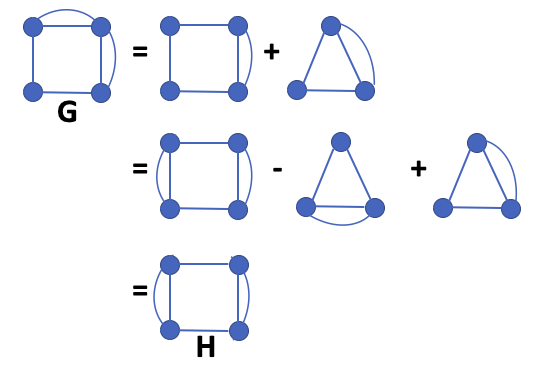
Figure 4: Certificate of Tutte Equivalence. Graph $G$ is Tutte Equivalent to Graph $H$.

The resulting certificate has the form:

$$G =G\setminus e+G/e~{}~{}~{}~{}~{}~{}~{}~{}\text{ (Applying {T1})}$$

$$=(G\setminus e+uv)-G\setminus e/uv+G/e~{}~{}~{}~{}~{}~{}~{}~{}\text{ (Applying {T2}})$$

$$=G\setminus e+uv~{}~{}~{}~{}~{}~{}~{}~{}\text{ (Algebraic Step (cancellation))}$$ (9)

where the graph $G\setminus e+uv\cong H$. If we replace each graph by its Tutte polynomial, each expression in the sequence is equal to the Tutte polynomial of $G$, and hence we have a certificate that shows that graphs $G$ and $H$ are Tutte equivalent.

Our work so far has focused on certificates of equivalence and factorisation. We expect that certificates could provide a graph-theoretic approach to studying other algebraic properties of graph polynomials.

In [83], Morgan introduced the concept of a schema or template for certificates of factorisation and equivalence. A schema specifies the structure of a certificate, including the relation to be applied at each step, but without filling in the actual graphs. So, instead of actual graphs (as in Figure 4), we just have symbols for them. In fact, as written — with symbols $G$, $G\setminus e$, etc. — (8) is really a schema for certificates, and the certificate in Figure 4 is one particular certificate that belongs to this schema.

In [87, 88], it was shown that every graph in a particular infinite family of strongly non-clique-separable graphs has a chromatic factorisation. Each certificate of factorisation in this family used the same sequence of certificate steps, so the entire infinite family of certificates could be described by a single schema.

If two graphs have the same multiset of blocks, then they are Tutte equivalent, since the Tutte polynomial is multiplicative over blocks. We can capture this multiplicativity in certificate steps that allow a graph to be replaced by a formal product of its blocks and vice versa.

[T3]:

$G\longrightarrow B_{1}B_{2}\cdots B_{k}$ where the $B_{i}$ are the blocks of $G$,

[T4]:

$B_{1}B_{2}\cdots B_{k}\longrightarrow G$ where $G$ is a graph with blocks $B_{i}$, $1\leq i\leq k$,

This enables us to write the following simple schema for certificates of Tutte equivalence for pairs of graphs with the same blocks.

$$G =\prod_{i=1}^{k}B_{i}~{}~{}~{}~{}~{}~{}~{}~{}\text{ (Applying {T3})}$$

$$=H~{}~{}~{}~{}~{}~{}~{}~{}\text{ (Applying {T4}).}$$ (10)

Effectively, this schema first ‘unglues’ blocks then ’glues’ them back together to produce graph $H$. This certificate schema works for all pairs of graphs that have the same blocks and may be regarded as a representation of the set of all such pairs.

Schemas 1 and 2 in [12] give two of the shortest certificates for pairs of chromatically equivalent graphs, $G$ and $H$. In both these schemas, graph $H$ can be obtained by removing an edge from graph $G$ and then adding a different edge.

Schema 2 relates pairs of chromatically equivalent graphs $G$ and $H$ with $G\setminus e\cong H\setminus f$ and $G/e\cong H/f$, where $e\in E(G)$ and $f\in E(H)$. Applying two deletion-contraction steps, we have:

$$G =G\setminus e-G/e$$

$$=(G\setminus e)+f$$ (11)

where $f\not\in E(G)$ and $G\setminus e+f\cong H$. The second step, (11), is obtained by rearranging the usual deletion-contraction relation.

Schema 1 is similar to Schema 2, but uses the addition-identification relation. Here $(G+e)\setminus f\cong H$. Applying two addition-identification steps, we have:

$$G =G+e+G/e$$

$$=(G+e)\setminus f$$ (12)

where $e\not\in E(G)$ and $f\in E(G)$.

More sophisticated certificates of equivalence are available. In [12], shortest certificates of chromatic equivalence are given for all pairs of chromatically equivalent graphs of order at most 7. These corresponded to 15 different schemas. It should be noted that a shortest certificate of equivalence may not be unique. In [84], infinitely many pairs of chromatically equivalent non-isomorphic graphs are constructed along with their certificates of equivalence.

The length of certificates has implications for the complexity of testing equivalence with respect to these polynomials (chromatic equivalence, Tutte equivalence, etc.). A short certificate of equivalence, once obtained, gives a means of verifying that two graphs have the same polynomial without computing the polynomial. For example, if the length of certificates of chromatic equivalence is polynomially bounded, then the problem of testing chromatic equivalence belongs to NP [12]. But at present we only have very loose, exponential upper bounds on certificate length. We discuss some implications of certificate length for the computational complexity of chromatic equivalence, factorisation and uniqueness in [12] and Tutte equivalence in [82].

Appropriate versions of certificates of equivalence and factorisation should be applicable to many other graph polynomials. We would like to see a rigorous theory of certificates of (at least) equivalence and factorisation for a broad class of graph polynomials with reduction relations. The commutativity of the operations of deleting/contracting different edges in a graph may be regarded as an instance of the Church-Rosser property from the theory of rewriting systems, as observed by Yetter [118] and Makowsky [70]; see also [7, result 9m, p. 72]. It seems to us that the theory of rewriting systems could shed more light on the kind of certificates we have considered here.

Acknowledgements

We thank Andrew Goodall, János Makowsky, Steven Noble and the referee for their comments. Through this Festschrift contribution, it is a pleasure to acknowledge János’s far-reaching contributions to the study of graph polynomials, through his mathematics and also through his generosity as a colleague, in sharing ideas, organising meetings and supporting the work of others.

References

- [1] J.L. Arocha and B. Llano, Mean value for the matching and dominating polynomial, Discussiones Mathematicae Graph Theory 20 (2000) 57–69.
- [2] J. Ashkin and E. Teller, Statistics of two-dimensional lattices with four components, Phys. Rev. 64 (1943) 178–184.
- [3] I. Averbouch, B. Godlin and J.A. Makowsky, A most general edge elimination polynomial, in: H. Broersma, T. Erlebach, T. Friedetzky and D. Paulusma (eds.), Graph-Theoretic Concepts In Computer Science: 34th Internat. Workshop (WG 2008) (Durham, UK, June/July 2008), Lecture Notes in Comput. Sci. 5344, Springer, Berlin, 2008, pp. 31–42.
- [4] I. Averbouch, B. Godlin and J.A. Makowsky, An extension of the bivariate chromatic polynomial, European J. Combin. 31 (1) (2010) 1–17.
- [5] L. Beaudin, J. Ellis-Monaghan, G. Pangborn and R. Shrock, A little statistical mechanics for the graph theorist, Discrete Math. 310 (2010) 2037–2053.
- [6] D. B. Benson, Life in the game of Go, Information Sciences 17 (1976) 17–29.
- [7] N. L. Biggs, Algebraic Graph Theory (2nd edn.), Cambridge University Press, 1993.
- [8] G. D. Birkhoff, A determinant formula for the number of ways of coloring a map, Ann. of Math. 14 (1912–1913) 42–46.
- [9] M. Bläser, H. Dell and J.A. Makowsky, Complexity of the Bollobás-Riordan polynomial. Exceptional points and uniform reductions, Theory Comput. Syst. 46 (4) (2010) 690–706.
- [10] A. Bohn, Chromatic roots as algebraic integers, 24th Internat. Conf. on Formal Power Series and Algebraic Combinatorics (FPSAC 2012) (Nagoya, Japan, 30 July – 3 Aug 2012), pp. 539–550.
- [11] L. Borzacchini and C. Pulito, On subgraph enumerating polynomials and Tutte polynomials, Boll. Un. Mat. Ital. B (6) 1 (1982) 589–597.
- [12] Z. Bukovac, G. Farr and K. Morgan, Short certificates for chromatic equivalence, Journal of Graph Algorithms and Applications 23 (2) (2019) 227–269.
- [13] P.J. Cameron, Cycle index, weight enumerator, and Tutte polynomial, Electron. J. Combin. 9 (2002) #N2 (10pp).
- [14] P.J. Cameron, Orbit counting and the Tutte polynomial, n: G. R. Grimmett and C. J. H. McDiarmid (eds.), Combinatorics, Complexity and Chance: A Tribute to Dominic Welsh, Oxford University Press, 2007, pp. 1–10.
- [15] P.J. Cameron, B. Jackson and J.D. Rudd, Orbit-counting polynomials for graphs and codes, Discrete Math. 308 (5–6) (2008) 920–930.
- [16] P.J. Cameron and K. Morgan, Algebraic properties of chromatic roots, Electronic J. Combinatorics 24 (2017) #P1.21.
- [17] S. Chmutov, Topological extensions of the Tutte polynomial, in: J. Ellis-Monaghan and I. Moffatt (eds.), Handbook on the Tutte Polynomial and Related Topics, Chapman and Hall/CRC Press, 2022, Chapter 27, pp. 497–513
- [18] B. Courcelle, J.A. Makowsky and U. Rotics, On the fixed parameter complexity of graph enumeration problems definable in monadic second-order logic, Discrete Appl. Math. 108 (1–2) (2001) 23–52.
- [19] P. de la Harpe and F. Jaeger, Chromatic invariants for finite graphs: theme and polynomial variations, Linear Algebra Appl. 226–228 (1995) 687–722.
- [20] D. Delbourgo and K. Morgan, Algebraic invariants arising from chromatic polynomials of theta graphs, Australasian Journal of Combinatorics 59 (2) (2014) 293–310.
- [21] A. de Mier Vinu’e, Graphs and Matroids Determined by their Tutte Polynomials, PhD thesis, Universitat Polit‘ecnica de Catalunya, 2003.
- [22] K. Dohmen, A. Pönitz and P. Tittmann, A new two-variable generalization of the chromatic polynomial, Discrete Mathematics and Theoretical Computer Science 6 (2003) 069–090.
- [23] J. Ellis-Monaghan, A. Goodall, J. A. Makowsky and I. Moffatt, Graph Polynomials: Towards a Comparative Theory (Dagstuhl Seminar 16241), in: Dagstuhl Reports (Schloss Dagstuhl - Leibniz-Zentrum für Informatik) 6 (6) (2016) 26–48. https://doi.org/10.4230/DagRep.6.6.26
- [24] J. Ellis-Monaghan, A. Goodall, I. Moffatt and K. Morgan, Comparative Theory for Graph Polynomials (Dagstuhl Seminar 19401), in: Dagstuhl Reports (Schloss Dagstuhl - Leibniz-Zentrum für Informatik) 9 (9) (2019) 135–155. https://doi.org/10.4230/DagRep.9.9.135
- [25] J. Ellis-Monaghan and I. Moffatt, Graphs on Surfaces: Dualities, Polynomials, and Knots, Springer, 2013.
- [26] J. Ellis-Monaghan and I. Moffatt (eds.), Handbook on the Tutte Polynomial and Related Topics, Chapman and Hall/CRC Press, 2022.
- [27] J. W. Essam, Graph theory and statistical physics, Discrete Math. 1 (1971) 83–112.
- [28] G. E. Farr, A correlation inequality involving stable set and chromatic polynomials, J. Combin. Theory (Ser. B) 58 (1993) 14–21.
- [29] G. E. Farr, A generalization of the Whitney rank generating function, Math. Proc. Camb. Phil. Soc. 113 (1993) 267–280.
- [30] G. E. Farr, On problems with short certificates, Acta Informatica 31 (1994) 479–502.
- [31] G. E. Farr, The Go polynomials of a graph, Theoretical Computer Science 306 (2003) 1–18.
- [32] G. E. Farr, Some results on generalised Whitney functions, Adv. in Appl. Math. 32 (2004) 239–262.
- [33] G. E. Farr, Tutte–Whitney polynomials: some history and generalizations, in: G. R. Grimmett and C. J. H. McDiarmid (eds.), Combinatorics, Complexity and Chance: A Tribute to Dominic Welsh, Oxford University Press, 2007, pp. 28–52.
- [34] G. E. Farr, On the Ashkin–Teller model and Tutte–Whitney functions, Combin. Probab. Comput. 16 (2007) 251–260.
- [35] G. E. Farr, Transforms and minors for binary functions, Ann. Combin. 17 (2013) 477–493.
- [36] G. E. Farr, The probabilistic method meets Go, Journal of the Korean Mathematical Society 54 (2017) 1121–1148.
- [37] G. E. Farr, Minors for alternating dimaps, Q. J. Math. 69 (2018) 285–320.
- [38] G. E. Farr, Binary functions, degeneracy, and alternating dimaps, Discrete Mathematics 342 (5) (2019) 1510–1519.
- [39] G. E. Farr, Using Go in teaching the theory of computation, SIGACT News 50 (1) (March 2019) 65–78.
- [40] G. E. Farr, The history of Tutte–Whitney polynomials, in: J. Ellis-Monaghan and I. Moffatt (eds.), Handbook on the Tutte Polynomial and Related Topics, Chapman and Hall/CRC Press, 2022, Chapter 34, pp. 623–668.
- [41] G. E. Farr, The forced colouring function of a graph, in preparation.
- [42] G. E. Farr and J. Schmidt, On the number of Go positions on lattice graphs, Information Processing Letters 105 (2008) 124–130.
- [43] S. Fiorini and R.J. Wilson, Edge-Colourings of Graphs, Research Notes in Mathematics 16, Pitman, 1977.
- [44] E. J. Farrell, An introduction to matching polynomials, J. Combin. Theory Ser. B 27 (1979) 75–86.
- [45] E. J. Farrell, On a class of polynomials associated with the cliques in a graph and its applications, Internat. J. Math. Math. Sci. 12 (1989) 77–84.
- [46] C. M. Fortuin and P. W. Kasteleyn, On the random cluster model. I. Introduction and relation to other models, Physica 57 (1972) 536–564.
- [47] F. Gavril, Algorithms on clique separable graphs, Discrete Math. 19 (1977) 159–165.
- [48] B. Godlin, E. Katz and J.A. Makowsky, Graph polynomials: from recursive definitions to subset expansion formulas, J. Logic Comput. 22 (2) (2012) 237–265.
- [49] C.D. Godsil and I. Gutman, On the theory of the matching polynomial, J. Graph Theory 5 (1981) 137–144..
- [50] A.J. Goodall, J. Nešetřil and P. Ossona de Mendez, Strongly polynomial sequences as interpretations, J. Appl. Logic 18 (2016) 129–149.
- [51] R. Greenlaw, H. J. Hoover and W. L. Ruzzo, Limits to Parallel Computation: P-Completeness Theory, Oxford University Press, 1995.
- [52] I. Gutman and F. Harary, Generalizations of the matching polynomial, Utilitas Mathematica 24 (1983) 97–106.
- [53] F. Harary and E. Palmer, Graphical Enumeration, Academic Press, New York, 1973.
- [54] O. J. Heilmann and E. H. Lieb, Monomers and dimers, Phys. Rev. Lett. 24 (25) (1970) 1412–1414.
- [55] T. Helgason, Aspects of the theory of hypermatroids, in: C. Berge and D. K. Ray-Chaudhuri (eds.), Hypergraph Seminar, Lecture Notes in Mathematics 411, Springer, Berlin, 1974, pp. 191–213.
- [56] S. Huggett, The Tutte polynomial and knot theory, in: J. Ellis-Monaghan and I. Moffatt (eds.), Handbook on the Tutte Polynomial and Related Topics, Chapman and Hall/CRC Press, 2022, Chapter 18, pp. 352–367.
- [57] T. Hunt, Milton Keynes Go Board, British Go Association, 30 April 2013. https://www.britgo.org/clubs/mk/mkboard.html
- [58] E. Ising, Beitrag zur Theorie des Ferromagnetismus, Z. Phys. 31 (1925) 253–258.
- [59] K. Iwamoto, Go for Beginners, Ishi Press, 1972, and Penguin Books, 1976.
- [60] T. Kotek, Definability of Combinatorial Functions, PhD thesis, Computer Science Department, Technion, 2012.
- [61] T.A. Kotek and J.A. Makowsky, The exact complexity of the Tutte polynomial, in: J. Ellis-Monaghan and I. Moffatt (eds.), Handbook on the Tutte Polynomial and Related Topics, Chapman and Hall/CRC Press, 2022, Chapter 9, pp. 175–193.
- [62] T.A. Kotek, J.A. Makowsky and E.V. Ravve, A computational framework for the study of partition functions and graph polynomials, in: R. Downey, J. Brendle, R. Goldblatt and B. Kim (eds.), Proc. 12th Asian Logic Conf. (Wellington, 15–20 December 2011), World Scientific, Hackensack, NJ, 2013, pp. 210–230.
- [63] T. Kotek, J.A. Makowsky and E.V. Ravve, On sequences of polynomials arising from graph invariants, European J. Combin. 67 (2018) 181–198.
- [64] T. Kotek, J.A. Makowsky and B. Zilber, On counting generalized colorings, in: M. Kaminski and S. Martini (eds.), Computer Science Logic: Proc. 22nd Internat. Workshop (CSL 2008), 17th Ann. Conf. of the EACSL (Bertinoro, 16–19 September 2008), Lecture Notes in Computer Science 5213, Springer, Berlin, 2008, pp. 339–353.
- [65] M. Lotz and J.A. Makowsky, On the algebraic complexity of some families of coloured Tutte polynomials, Adv. in Appl. Math. 32 (1–2) (2004) 327–349.
- [66] T. Krajewski, I. Moffatt and A. Tanasa, Hopf algebras and Tutte polynomials, Adv. in Appl. Math. 95 (2018) 271–330.
- [67] J.A. Makowsky, Algorithmic uses of the Feferman–Vaught Theorem, Annals of Pure and Applied Logic 126 (2004) 159–213.
- [68] J.A. Makowsky, Coloured Tutte polynomials and Kauffman brackets for graphs of bounded tree width, Discrete Appl. Math. 145 (2) (2005) 276–290.
- [69] J.A. Makowsky, From a zoo to a zoology: descriptive complexity for graph polynomials, in: A. Beckmann, U. Berger, B. Löwe, and J.V. Tucker (eds.), Logical Approaches to Computational Barriers, Second Conference on Computability in Europe, CiE 2006 (Swansea, UK, July 2006), Lecture Notes in Computer Science 3988, Springer, 2006, pp. 330–341.
- [70] J.A. Makowsky, From a zoo to a zoology: towards a general theory of graph polynomials, Theory of Computing Systems 43 (2008) 542–562.
- [71] J.A. Makowsky, The graph polynomials project in Haifa, https://janos.cs.technion.ac.il/RESEARCH/gp-homepage.html [accessed 23 February 2024].
- [72] J.A. Makowsky, How I got to like graph polynomials, arXiv preprint, 6 September 2023, http://arxiv.org/abs/2309.02933v1.
- [73] J.A. Makowsky, Meta-theorems for graph polynomials, to appear.
- [74] J.A. Makowsky and J.P. Mariño, Farrell polynomials on graphs of bounded tree width, Adv. in Appl. Math. 30 (1–2) (2003) 160–176.
- [75] J.A. Makowsky and K. Meer, On the complexity of combinatorial and metafinite generating functions of graph properties in the computational model of Blum, Shub and Smale, in: P.G. Clote and H. Schwichtenberg (eds.), Computer Science Logic: Proc. 14th Internat. Workshop (CSL 2000), Ann. Conf. of the EACSL (Fischbachau, 21–26 August 2000), Lecture Notes in Computer Science 1862, Springer-Verlag, Berlin, 2000, pp. 399–410.
- [76] J.A. Makowsky and E.V. Ravve, Semantic equivalence of graph polynomials definable in second order logic, in: Jouko Väänänen, Å. Hirvonen and R. de Queiroz (eds.), Logic, Language, Information, and Computation: Proc. 23rd Internat. Workshop (WoLLIC 2016) (Benemérita Universidad Autónoma de Puebla, Puebla, 16–19 August 2016), Lecture Notes in Comput. Sci. 9803, Springer-Verlag, Berlin, 2016, pp. 279–296.
- [77] J.A. Makowsky, E.V. Ravve and N.K. Blanchard, On the location of roots of graph polynomials, European J. Combin. 41 (2014) 1–19.
- [78] J.A. Makowsky, E.V. Ravve and T. Kotek, A logician’s view of graph polynomials, Annals of Pure and Applied Logic 170 (2019) 1030–1069.
- [79] P. Martin, Anneau de Tutte–Grothendieck associé aux dénombrements eulériens dans les graphes 4-réguliers planaires, Colloque sur la Théorie des Graphes (Brussels, 1973), Cahiers Centre Études Recherche Opér. 15 (1973) 343–349.
- [80] C. Merino, A. de Mier and M. Noy, Irreducibility of the Tutte polynomial of a connected matroid, Journal of Combinatorial Theory 83 (2001) 298–304.
- [81] R Mo, G Farr and K Morgan, Certificates for properties of stability polynomials of graphs, Electronic Journal of Combinatorics 21 (2014), #P1.66 (25pp).
- [82] R. Mo, K. Morgan and G. Farr, Certificates for Tutte equivalence, to be submitted.
- [83] K. Morgan, Algebraic aspects of the chromatic polynomial, PhD thesis, Monash University, 2010. https://doi.org/10.4225/03/587852a8b487b
- [84] K. Morgan, Pairs of chromatically equivalent graphs, Graphs and Combinatorics 27 (4) (2010) 547–556.
- [85] K. Morgan, Galois groups of chromatic polynomials, LMS J. Comput. Math. 15 (2012) 281–307.
- [86] K. Morgan and R. Chen, An infinite family of 2-connected graphs that have reliability factorisations, Discrete Applied Mathematics 218 (2017) 123–127.
- [87] K. Morgan and G. Farr, Certificates of factorisation for chromatic polynomials, Electron. J. Combin. 16 (2009) #R74 (29pp).
- [88] K. Morgan and G. Farr, Certificates of factorisation for a class of triangle-free graphs, Electron. J. Combin. 16 (2009) #R75 (14pp).
- [89] K. Morgan and G. Farr, Non-bipartite chromatic factors, Discrete Mathematics 312 (2012) 1166–1170.
- [90] M. Morse, George David Birkhoff and his mathematical work, Bull. Amer. Math. Soc. 52 (1946) 357–391.
- [91] S. D. Noble, The , V, and polynomials, in: J. Ellis-Monaghan and I. Moffatt (eds.), Handbook on the Tutte Polynomial and Related Topics, Chapman and Hall/CRC Press, 2022, Chapter 26, pp. 7733–496.
- [92] S. D. Noble and D. J. A. Welsh, A weighted graph polynomial from chromatic invariants of knots, Ann. Inst. Fourier (Grenoble) 49 (3) (1999) 1057–1087.
- [93] J. G. Oxley and G. P. Whittle, Tutte invariants for -polymatroids, in: N. Robertson and P. D. Seymour (eds.), Graph Structure Theory (Seattle, 1991), Contemp. Math. 147, Amer. Math. Soc., Providence, RI, 1993, pp. 9–19.
- [94] J. Oxley and G. Whittle, A characterization of Tutte invariants of 2-polymatroids, J. Combin. Theory Ser. B 59 (1993) 210–244.
- [95] G. Pólya, Kombinatorische Anzahlbestimmungen für Gruppen, Graphen und chemische Verbindungen, Acta Math. 68 (1937) 145–254.
- [96] R. B. Potts, Some generalized order-disorder transformations, Proc. Camb. Phil. Soc. 48 (1952) 106–109.
- [97] H. Redfield, The theory of group-reduced distributions, Amer. J. Math. 49 (1927) 433–455.
- [98] H. Segerman, Diamond Go, http://www.segerman.org/diamond/.
- [99] Sensei’s Library, Tromp-Taylor Rules, https://senseis.xmp.net/?TrompTaylorRules [accessed 19 February 2024].
- [100] R. P. Stanley, Acyclic orientations of graphs, Discrete Math. 5 (1973) 171–178.
- [101] E. Thorp and W.E. Walden, A partial analysis of Go, Computer J. 7 (3) (1964) 203–207.
- [102] E. Thorp and W.E. Walden, A computer assisted study of Go on boards, Information Sciences 4 (1) (1972) 1–33.
- [103] P. Tittmann, Graph Polynomials: The Eternal Book, 14 February 2024. https://www.researchgate.net/publication/377572474_Graph_Polynomials_The_Eternal_Book
- [104] M. Trinks, The covered components polynomial: a new representation of the edge elimination polynomial, Electron. J. Combin. 19 (2012) #P50 (31pp).
- [105] J. Tromp and W. Taylor, The game of Go, https://tromp.github.io/go.html [accessed 19 February 2024].
- [106] W. T. Tutte, A ring in graph theory, Proc. Camb. Phil. Soc. 43 (1947) 26–40.
- [107] W. T. Tutte, A contribution to the theory of chromatic polynomials, Canadian J. Math. 6 (1954) 80–91.
- [108] W. T. Tutte, On dichromatic polynomials, J. Combin. Theory 2 (1967) 301–320.
- [109] W. T. Tutte, Codichromatic graphs, J. Combin. Theory Ser. B 16 (1974) 168–174.
- [110] W. T. Tutte, Graph Theory as I Have Known It, Oxford, 1998.
- [111] W. T. Tutte, Graph-polynomials, Adv. in Appl. Math. 32 (2004) 5–9.
- [112] R. Van Slyke and H. Frank, Network reliability analysis. I., Networks 1 (1971/72), 279–290.
- [113] D. J. A. Welsh, Matroid Theory, London Math. Soc. Monograph No. 8, Academic Press, London, 1976.
- [114] D. J. A. Welsh, Complexity: Knots, Colourings and Counting, London Math. Soc. Lecture Note Series 186, Cambridge University Press, 1993.
- [115] H. Whitney, The Coloring of Graphs, PhD thesis, Harvard University, 1932.
- [116] H. Whitney, The coloring of graphs, Ann. of Math. (2) 33 (1932) 688–718.
- [117] H. Whitney, A set of topological invariants for graphs, Amer. J. Math. 55 (1933) 231–235.
- [118] D. N. Yetter, On graph invariants given by linear recurrence relations, J. Combin. Theory (Ser. B) 48 (1990) 6–18.
- [119] A. A. Zykov, On some properties of linear complexes (in Russian), Math. Sbornik 24 (1949) 163–188. English translation: Amer. Math. Soc. Transl. 79 (1952).
- [120] A. A. Zykov, Recursively calculable functions of graphs, in: Theory of Graphs and its Applications (Proc. Sympos. Smolenice, 1963), Publ. House Czechoslovak Acad. Sci., Prague, 1964, pp. 99–105.