Hecke operators on rational functions II

Abstract.

We study the action of the Hecke operators $U_{n}$ on the space $\mathcal{R}$ of rational functions of one variable, over $\mathbb{C}$. The main goal is to give a complete classification of the eigenfunctions of $U_{n}$, answering many questions that were set out in [4]. We accomplish this by introducing certain number-theoretic directed graphs, called Zolotarev Graphs, which extend the well-known permutations due to Zolotarev.

We develop the theory of the Zolotarev graphs, and discover certain strong relations between these graphs and the kernel of $U_{n}$ acting on a subspace of $\mathcal{R}$. We decompose the eigenfunctions of $U_{n}$ into certain natural finite-dimensional vector spaces of rational functions, which we call the eigenspaces. In this context, we prove that the dimension of each eigenspace is equal to the number of nodes of its corresponding Zolotarev graph, belonging to a cycle. We prove that the number of leaves of this Zolotarev graph equals the dimension of the kernel of $U_{n}$. We then give a novel number-theoretic formula for the number of cycles of fixed length, in each Zolotarev graph. We also study the simultaneous eigenfunctions for all of the $U_{n}$, and give explicit bases for all of them. Finally, we prove that the classical Artin Conjecture on primitive roots is equivalent to the conjecture that infinitely many of these eigenspaces have dimension $1$.

1. Introduction

A very useful linear operator in Number theory is the series dissection operator:

(1) $$U_{n}\left(\sum_{k=0}^{\infty}a(k)x^{k}\right):=\sum_{k=0}^{\infty}a(nk)x^{k},$$

where $n$ is any fixed positive integer. The operator $U_{n}$ was thoroughly studied by Hecke in the important case that the series in (1) represents a modular form, and is therefore called a Hecke operator (see [1] for Erich Hecke´s original paper). In other contexts such operators are also called dissection operators, because they pick out every $n$’th coefficient of the series.

Given a positive integer $n$, here we study the action of $U_{n}$ on the vector space of rational functions over $\mathbb{C}$ that are analytic at the origin:

(2) $$\mathcal{R}:=\left\{\frac{p(x)}{q(x)}\mid p,q\in\mathbb{C}[x]\text{ and }\frac{p(x)}{q(x)}=\sum_{k=0}^{\infty}a(k)x^{k},\text{ near the origin}\right\}.$$

The operator $U_{n}$ acts on the vector space $\mathcal{R}$, sending a rational function to another rational function (see [4]). It follows easily from its definition that $U_{n}$ is a linear operator.

Our first main goal is to give an explicit description of all the rational functions in $\mathcal{R}$ that are eigenfunctions of $U_{n}$:

(3) $$U_{n}f(x)=\lambda f(x),$$

for all $x$ near the origin. For each $n\in\mathbb{Z}_{>0}$, there are always rational eigenfunctions of $U_{n}$, for example the trivial eigenfunction $f(x):=\frac{1}{1-x}=\sum_{k\geq 0}x^{n}$, which satisfies (3). In [4], we studied and classified the eigenvalues of the Hecke operators $U_{n}$, on the space of rational functions with real coefficients, but [4] did not classify the eigenfunctions. Here we extend this study by completely classifying all of the eigenfunctions of $U_{n}$, as well as working more generally over $\mathbb{C}$.

Our second main goal is to introduce and study the related number-theoretic graphs, which we call Zolotarev graphs (Section 2), which we use to classify the eigenfunctions of $U_{n}$, for all positive integers $n$.

Our final objective is to restate the Artin Conjecture on primitive roots in terms of one-dimensional eigenspaces.

Theorem 1.

Fix a positive integer $n>1$, and let $f\in\mathcal{R}$ be an eigenfunction of $U_{n}$ with $n>1$ and eigenvalue $\lambda\neq 0$. Then all of the poles of $f$ are roots of unity.

(Proof) $\square$

By Theorem 1, there is a least positive integer $L$ such that the poles of $f$ are all $L$’th roots of unity. We call this unique $L$ the level of $f$, and we will sometimes use the notation $\rm{level}(f)=L$.

Lemma 1.

Suppose $f\in\mathcal{R}$ is an eigenfunction of $U_{n}$, with $n>1$, such that $f$ has level $L$, and eigenvalue $\lambda\neq 0$. Then $\gcd(n,L)=1$.

(Proof) $\square$

Theorem 2.

Fix a positive integer $n>1$, and let $f\in\mathcal{R}$ be an eigenfunction of $U_{n}$, with eigenvalue $\lambda\not=0$. Then all the poles of $f$ have the same multiplicity, which we denote by $\kappa$.

(Proof) $\square$

Moreover, under the assumption of Theorem 2, we call the unique nonnegative integer $\kappa$ the weight of $f$, and write $\rm{weight}(f)=\kappa$. We first observe an interesting relation between $n$ and the level $L$ of an eigenfunction.

Now it makes sense to work with the order of $n$ modulo $L$, which we denote throughout by

$$c:={\rm ord}_{L}(n).$$

Theorem 3.

Fix a positive integer $n>1$, and let $f\in\mathcal{R}$ be an eigenfunction of $U_{n}$. If we have $U_{n}f(x)=\lambda f(x)$, for a nonzero eigenvalue $\lambda$, then

$$\lambda=\omega\,n^{\kappa-1},$$

where

$$\omega:=e^{\frac{2\pi im}{c}},$$

for some integer $m$. Here $\rm{weight}(f)=\kappa$, and ${\rm level}(f)=L$.

(Proof) $\square$

Corollary 1.

For each integer $n>1$, the eigenfunctions $f(x)$ of $U_{n}$ with eigenvalue $\lambda\neq 0$, level $L$ and weight $\kappa$ may be written as

$$f(x)=\sum_{k=0}^{\infty}k^{\kappa-1}a(k)x^{k}$$

where $a$ is a periodic function on $\mathbb{Z}_{\geq 0}$, with smallest period $L$. (Proof) $\square$

Corollary 2.

The spectrum of the operator $U_{n}$, acting on $\mathcal{R}$, is:

(4) $${\rm Spec}(U_{n})=\{e^{\frac{2\pi im}{c}}n^{\kappa-1}\mid m\in\mathbb{Z},\text{ and }\kappa,L\text{ are positive integers},(n,L)=1\},$$

where $c:={\rm ord}_{L}(n)$. (Proof) $\square$

Corollary 3.

If $N$ lies in the image of Euler’s totient function $\phi$, then $\lambda=e^{\frac{2\pi i}{N}}$ is an eigenvalue of $U_{n}$. (Proof) $\square$

The converse of Corollary 3 is false (see Remark (d)).

The latter Corollary 1 strongly suggests that we consider the following natural subspace of $\mathcal{R}$:

(5) $$\mathcal{R}(L,\kappa):=\left\{f\in\mathcal{R}\mid f(x)=\sum_{k\geq 0}k^{\kappa-1}a(k)x^{k},\text{ where }a(k+L)=a(k)\right\},$$

which also contains functions that are not eigenfunctions of any $U_{n}$. We note that if $L_{1}\mid L_{2}$, then $\mathcal{R}(L_{1},\kappa)\subseteq\mathcal{R}(L_{2},\kappa).$ Throughout, we’ll use the following useful notation.

Definition 1.

The indicator function of an arithmetic progression $\{a+nL\mid n\in\mathbb{Z}\}$ is defined by:

(6) $$1_{a\text{ mod }L}(x):=\begin{cases}0&\text{ if }x\not\equiv a\ \left(\mathrm{mod}\ L\right)\\ 1&\text{ if }x\equiv a\ \left(\mathrm{mod}\ L\right).\end{cases}$$

Lemma 2.

$\mathcal{R}(L,\kappa)$ is a vector space with $\dim\mathcal{R}(L,\kappa)=L.$ (Proof) $\square$

We fix two positive integers $\kappa$ and $L$. For each given root of unity $\omega\in\mathbb{C}$, we consider the eigenspace corresponding to $\omega$:

(7) $$E_{n}(\omega,L,\kappa):=\left\{f\in\mathcal{R}\mid U_{n}(f)=n^{\kappa-1}\omega f,\text{ where }\text{level}(f)\mid L,\text{and weight}(f)=\kappa\right\}.$$

We observe that if $L_{1}\mid L_{2}$, then $E_{n}(\omega,L_{1},\kappa)\subseteq E_{n}(\omega,L_{2},\kappa)$, because

$$E_{n}(\omega,L,\kappa)=\left\{f\in\mathcal{R}(L,\kappa)\mid U_{n}(f)=n^{\kappa-1}\omega f\right\}.$$

Each vector space $E_{n}(\omega,L,\kappa)$ is a convenient packet of eigenfunctions of $U_{n}$. It’ll turn out that $E_{n}(\omega,L,\kappa)$ forms a very interesting finite dimensional vector space, whose elements have number-theoretic content. To describe the rational eigenfunctions of $U_{n}$, we’ll develop some special permutations first.

1.1. Zolotarev permutations

There are some natural permutations that we study here, which naturally arise in the study of the eigenfunctions of Hecke operators. Throughout this section, we let $n,L\in\mathbb{Z}_{>0}$, $\left(n,L\right)=1$, and $c:={\rm ord}_{L}(n)$. Consider the map that sends each element $m\in\mathbb{Z}/L\mathbb{Z}$ to $mn\pmod{L}$. We will write $\overline{mn}$ for the unique integer in the interval $[0,L-1]$ that is congruent to $mn\pmod{L}$. Because $(n,L)=1$, this map is a permutation of $\mathbb{Z}/L\mathbb{Z}$, which we may write as:

(8) $$\tau(n,L):=\begin{pmatrix}0&1&\cdots&k&\cdots&L-1\\ &&&&&\\ \overline{0}&\overline{n}&\cdots&\overline{kn}&\cdots&\overline{(L-1)n}\end{pmatrix},$$

which we’ll call a Zolotarev permutation, because these permutations were used by Zolotarev to prove the reciprocity laws of Gauss and of Jacobi.

The permutation $\tau(n,L)$ breaks up into a product of disjoint cycles (called the disjoint cycle decomposition) where for each $1\leq j\leq c$, we define

(9) $$b_{j}:=\text{ the number of disjoint cycles of length }j,\text{ in }\tau(n,L).$$

Of course, we allow $b_{j}=0$ to hold as well. We note that there always exists the following cycle in the permutation $\tau(n,L)$: $(1\rightarrow\overline{n}\rightarrow\overline{n}^{2}\rightarrow\cdots\overline{n}^{c-1})$. Zolotarev permutations have also been studied in [2], for example, in the context of cyclotomic cosets.

Example 1.

Let $L=30$, and $n=7$. It’s easy to check that ${\rm ord}_{30}(7)=4$. Here (8) has the disjoint cycle decomposition:

$$\tau(7,30)=(1\ 7\ 19\ 13)(2\ 14\ 8\ 26)(3\ 21\ 27\ 9)(4\ 28\ 16\ 22)(6\ 12\ 24\ 18)(11\ 17\ 29\ 23)(0)(5)(10)(15)(20)(25).$$

Therefore $b_{1}=6$, $b_{2}=b_{3}=0$, and $b_{4}=6$. $\square$

It is natural to ask: does there exist some nice formula for $b_{j}$?

Lemma 3.

We fix positive integers $n,L$. Then the number of cycles of length $j$ in $\tau(n,L)$ is given by

(10) $$b_{j}=\frac{1}{j}\sum_{d\mid j}\mu\left(\frac{j}{d}\right)\gcd(n^{d}-1,L).$$

(Proof) $\square$

We observe that the proof of Lemma 3 does not require $n$ to be coprime to $L$. This suggests a more general theory than Zolotarev permutations, which we call Zolotarev graphs, and which form an integral part of our study of eigenfunctions of $U_{n}$, beginning with Section 2.

Example 2.

We’ve already seen that $b_{1}=\gcd(n,L-1)$, by Lemma 3. If $L:=p$, a prime, then all cycles in $\tau(n,L)$ must have a length that divides $\phi(p)=p-1$. It follows that when we calculate $b_{j}$, we must have $j\mid p-1$. By Lemma 3, we have:

(11) $$b_{j}=\frac{1}{j}\sum_{d\mid j}\mu\left(\frac{j}{d}\right)\gcd(n^{d}-1,p),$$

for each $j\mid p-1$. To see a special case, we let $L=17,n=2$. Then $j|16\implies j\in\{1,2,4,8,16\}$. Using (11), we may compute the nonzero $b_{j}$:  $b_{1}=\gcd(n-1,17)=1,\ b_{2}=\tfrac{1}{2}\sum_{d\mid 2}\mu\left(\frac{2}{d}\right)\gcd(2^{d}-1,17)=0,\ b_{4}=0,b_{8}=2$, and $b_{16}=0$. $\square$

Lemma 4.

Given positive coprime integers $L,n$, let $c:={\rm ord}_{L}(n)$. Then the Zolotarev permutations enjoy the following properties:

1. if $\overline{c}$ is the size of a cycle, then $\overline{c}\mid c$.

2. Let $A$ and $B$ be cycles in $\tau(n,L)$. Then, $A$ and $B$ are distinct $\iff$ $A\cap B=\varnothing$.

3. $\sum_{j=1}^{c}jb_{j}=L$.

(Proof) $\square$

1.2. Remarks

1. We note that the proof of Lemma 3 uses the elementary fact that $L\mid k(n^{j}-1)\iff\frac{L}{\gcd(n^{j}-1,L)}\mid k.$ But the latter statement is also equivalent to $\frac{L}{(L,k)}\mid n^{j}-1$, which gives us another way to calculate $b_{j}$, as follows.

   (12) $$b_{j}=\frac{1}{j}\left|\left\{1\leq m\leq L\mid j={\rm ord}_{\frac{L}{(L,m)}}(n)\right\}\right|.$$

2. Equation (12) also gives the following identity:

   $$\sum_{d\mid j}\mu\left(\frac{j}{d}\right)\gcd(n^{d}-1,L)=\left|\left\{1\leq m\leq L\mid j={\rm ord}_{\frac{L}{(L,m)}}(n)\right\}\right|.$$

3. Suppose we fix an eigenfunction $f\in E_{n}(\omega,L,\kappa)$, with an eigenvalue $\lambda=n^{\kappa-1}\omega$, where $\omega$ is a root of unity. Then using the notation of Theorem 3 we know that:

   $$\frac{\lambda}{n^{\kappa-1}}=\omega=e^{\frac{2\pi im/\gcd(m,c)}{c/\gcd(m,c)}}:=e^{\frac{2\pi im/\gcd(m,c)}{h}},$$

   where $h:=\frac{c}{\gcd(m,c)}=\frac{{\rm ord}_{L}(n)}{\gcd(m,c)}={\rm ord}_{L}(n^{m})$.

4. The converse to Corollary 3 does not hold. Indeed, consider $U_{2}:\mathcal{R}(29,1)\rightarrow\mathcal{R}(29,1)$. By means of an easy computation, we verify that $2$ is a primitive root modulo 29, thus ${\rm ord}_{29}(2^{2})={\rm ord}_{29}(4)=14.$ Therefore, by Corollary 2, $e^{\frac{2\pi i}{14}}\in\text{Spec}(U_{2})$. On the other hand, [13] shows that the equation $\phi(x)=14$ does not admit a solution.

2. Zolotarev graphs

To completely characterize the eigenspaces given by $U_{n}$ acting on $\mathcal{R}(L,\kappa)$, including its kernel, we must extend the Zolotarev permutations to any two integers $n$, $L$, not necessarily coprime. The fact that we do not require $n$ and $L$ to be coprime in the proof of Lemma 3 already foreshadows a generalization of the Zolotarev permutations.

We now introduce the Zolotarev graphs. In the followings sections, we will use this strong tool to paint a more complete picture of the eigenspaces of $U_{n}$, and of its kernel.

Definition 2.

Let $Z(n,L)$ be the directed graph whose nodes are given by the integers in $\mathbb{Z}/L\mathbb{Z}$, and such that there exists a directed edge from vertex $a$ to vertex $b$ precisely when $na\equiv b\ \left(\mathrm{mod}\ L\right)$. We’ll often use the notation $a\longmapsto b$ and call such a directed graph a Zolotarev graph.

So the Zolotarev permutations, defined by (8), are now replaced by Zolotarev graphs above. Given a Zolotarev graph $Z(n,L)$, we define the following terms, for any $m\in\mathbb{Z}/L\mathbb{Z}$:

1. $m$ is called a leaf integer if there does not exist an integer $k$ such that $nk\equiv m\ \left(\mathrm{mod}\ L\right)$, i.e., the indegree of $m$ is 0.

2. $m$ is called a root integer if there exists an integer $k$ such that $n^{k}m\equiv m\ \left(\mathrm{mod}\ L\right)$.

3. $m$ is called a branch integer if it is neither a leaf, nor a root.

For simplicity, each integer in $m\in\mathbb{Z}/L\mathbb{Z}$ will simply be called a leaf, a root, or a branch. From these definitions, it follows that the sum of the number of leaves, roots and branches in $Z(n,L)$ is precisely equal to $L$.

Definition 3.

A directed path of length $N$ is a sequence of vertices $m_{1},m_{2},\cdots,m_{N}\in Z(n,L)$, such that there is a directed edge between $m_{i}$ and $m_{i+1}$, for all $i=1,2,\dots,N-1$.

We may also consider the undirected graph $G(n,L)$ that is defined by using the same data of $Z(n,L)$, but simply ignoring the directions on each edge. We consider a maximal set of vertices in $G(n,L)$ such that for each $2$ of its vertices $a,b$, we have an undirected path between $a$ and $b$. The subgraph of $G(n,L)$, induced by these vertices, defines a connected component of $G(n,L)$.

Definition 4.

We define a connected component of $Z(n,L)$ by taking a connected component of $G(n,L)$, and including the original direction on each of its edges.

Example 3.

In Figure 1, we see the Zolotarev graphs $Z(10,20)$, which has just $1$ connected component, $1$ root, $1$ branch, and $18$ leaves. We also see the Zolotarev graph $Z(14,20)$, which has $3$ connected components, $5$ roots, $5$ branches, and $10$ leaves. We note that the indegree of a node that is not a leaf in $Z(14,20)$ is equal to $(14,20)=2$, and the indegree of a node that is not a leaf in $Z(10,20)$ is equal to $(10,20)=10$.

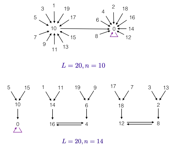
Figure 1. Above: the Zolotarev graph $Z(10,20)$. Below: the Zolotarev graph $Z(14,20)$.

See appendix B for all of the Zolotarev Graphs with $L=20.$

Throughout, we will also use the following important function of $L$ and $n$.

Definition 5.

For any two positive integers $L,n$, we let

(13) $$L_{n}:=\text{ the largest divisor of }L\text{ that is coprime with }n.$$

Example 4.

Let $L=40$, and $n=4$. Here $L_{n}=5$. We note that there is an alternative algorithm to compute $L_{n}$. Namely, we may define $x_{1}:=\frac{L}{\gcd(L,n)}$, and inductively define $x_{j}:=\frac{x_{j-1}}{\gcd(x_{j-1},n)}$. Then it’s an easy exercise to show that after a finite number of steps this sequence converges to $L_{n}$. In this example, we have $x_{1}=10$, $x_{2}=5$, and $L_{n}=5$. $\square$

2.1. Structure of the Zolotarev graphs

Definition 6.

Given a Zolotarev Graph $Z(n,L)$ and a root $m$, a cycle of length $j$, containing $m$ (if it exists), is the set

$$A=\{m\cdot n^{k}\mid k\in\mathbb{Z}\},\text{ with }|A|=j.$$

We note that it follows easily from the definitions above that each connected component of $Z(n,L)$ contains exactly one cycle.

Observation 1.

Let $n,L$ be positive integers. Then the number of cycles of length $j$ in $Z(n,L)$ is given by

(14) $$b_{j}=\frac{1}{j}\sum_{d\mid j}\mu\left(\frac{j}{d}\right)\gcd(n^{d}-1,L).$$

We remark that the proof of this observation follows directly from the proof of Lemma 3, since it does not rely on any assumption about the greatest common divisor of $n$ and $L$.

Observation 2.

There are

$$\sum_{j=1}^{L}\frac{1}{j}\sum_{d\mid j}\mu\left(\frac{j}{d}\right)\gcd(n^{d}-1,L).$$

connected components in $Z(n,L)$.

This follows directly from equation (14). $\square$

Example 5.

Let’s compute $b_{j}$, the number of cycles of length $j$, in $Z(2,20)$. By Lemma 1, we compute the following $b_{j}$ values: $b_{1}=\gcd(2-1,20)=1$, $b_{2}=\frac{1}{2}\sum_{d\mid 2}\mu\left(\frac{2}{d}\right)\gcd(2^{d}-1,20)=0$,

$$b_{4}=\frac{1}{4}\sum_{d\mid 4}\mu\left(\frac{4}{d}\right)\gcd(2^{d}-1,20)=\frac{1}{4}\left(-\gcd(2^{2}-1,20)+\gcd(2^{4}-1,20)\right)=1.$$

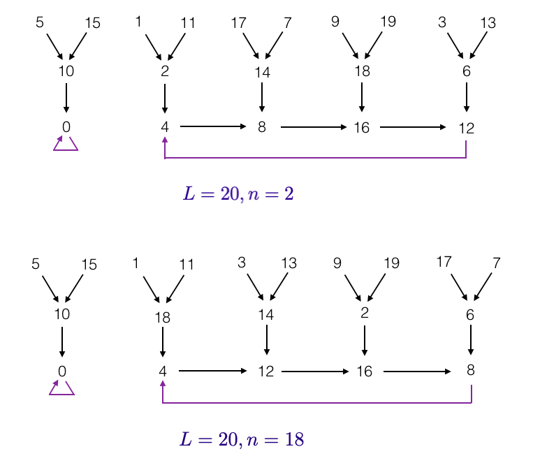
Figure 3. The two Zolotarev graphs $Z(2,20)$ and $Z(18,20)$ are isomorphic. Each of these graphs has $10$ leaves, $5$ branches, $5$ roots, and $2$ connected components.

We also have $b_{j}=0$ for all other values of $j$, and the latter data confirms our data from Figure 3. $\square$

Lemma 5.

Suppose that $k\in Z(n,L)$ is not a leaf, and $g:=\gcd(n,L)$. Then, the $g$ solutions to $n\cdot c\equiv k\ \left(\mathrm{mod}\ L\right)$ are all congruent to a fixed $c$ mod $\frac{L}{g}$.

(Proof) $\square$

We observe that all nodes that are not leaves have the same indegree $(n,L)$.

Theorem 4.

If $(L,n)>1$ and $Z(n,L)$ is a Zolotarev graph, the following hold:

1. $m$ is a leaf $\iff$ $(n,L)\nmid m$

2. $m$ is a root $\iff$ $\frac{L}{L_{n}}\mid m$

3. $m$ is a branch $\iff$ $(n,L)\mid m$ and $\frac{L}{L_{n}}\nmid m$

(Proof) $\square$

Corollary 4.

Any Zolotarev graph $Z(n,L)$ has precisely:

1. $L_{n}$ roots.

2. $L-\frac{L}{(n,L)}=L\frac{(n,L)-1}{(n,L)}$ leaves.

3. $\frac{L}{(n,L)}-L_{n}$ branches.

(Proof) $\square$

We’ll show in Section 6 below that the dimension of the kernel of $U_{n}$ acting on $\mathcal{R}(L,\kappa)$ is equal to the number of leaves of $Z(n,L).$

Lemma 6.

If $m\in Z(n,L)$, then exists a unique integer $k$, with $0\leq k<\frac{L}{L_{n}}$ such that $m+kL_{n}$ is a root. (Proof) $\square$

Theorem 5.

The number of roots of a Zolotarev graph $Z(n,L)$ is equal to $\sum_{j=1}^{L}{jb_{j}}$, and may be expressed as follows:

(15) $$|roots|=\sum_{j=1}^{L}\sum_{d\mid j}\mu\left(\frac{j}{d}\right)\gcd(n^{d}-1,L).$$

(Proof) $\square$

Therefore, by Corollary 4, we obtain an explicit formula for $L_{n}$:

(16) $$L_{n}=\sum_{j=1}^{L}\sum_{d\mid j}\mu\left(\frac{j}{d}\right)\gcd(n^{d}-1,L).$$

$\square$

Definition 7.

We define the distance between any two nodes $a,b$ of $Z(n,L)$, to be the smallest integer $k$ that satisfies $n^{k}a\equiv b\mod L$, if such a $k$ exists and we write $d(a,b)=k$. In case the latter congruence does not have a solution, we say that $d(a,b)=\infty$.

In particular, we note that $d(a,a)=0$, for all $a\in Z(n,L)$.

Definition 8.

Given any root $r$ of $Z(n,L)$, we consider the directed tree above $r$, which we call ${\rm Tree}(r)$, whose vertices are the integers $m\in\mathbb{Z}/L\mathbb{Z}$, such that there exists a directed path from $m$ to $r$ which does not contain any other roots. We note that $r\in{\rm Tree}(r)$.

Theorem 6.

$k\in{\rm Tree}(0)\iff L_{n}\mid k$. Also, $d(L_{n},0)\geq d(k\cdot L_{n},0)$, with equality when $(k,n)=1.$

(Proof) $\square$

Theorem 7.

Suppose $i\in Z(n,L)$ is a root contained in a cycle of size $j$ and let $a$ and $b$ be any two nodes in the same connected component as $i$. Then

$$a\equiv b\ \left(\mathrm{mod}\ L_{n}\right)\iff d(a,i)\equiv d(b,i)\ \left(\mathrm{mod}\ j\right).$$

(Proof) $\square$

Definition 9.

The height $H(m)$ of a node $m\in Z(n,L)$ is the smallest distance between $m$ and any root of $Z(n,L)$. We say that a Zolotarev graph $Z(n,L)$ has homogeneous height $h$ if all the leaves have the same height $h$. We say $Z(n,L)$ has height $h$, if $h$ is equal to the maximum height of any leaf of the graph.

Lemma 7.

If $Z(n,L)$ has height $h$, then $h=H(1)$. (Proof) $\square$

We can therefore denote the height of $Z(n,L)$ by $H(1)$.

Theorem 8.

$Z(n,L)$ has homogeneous height $h$ $\iff$ $L_{n}=\frac{L}{(n,L)^{h}}$.

(Proof) $\square$

This formula reminds the first way to calculate $L_{n}$ described in Example 4. We will note that it is not an coincidence and also the structure of the height of the leaves is strongly related with the recursive calculation of $L_{n}$ like in 4, as we will see in Corollary 6

2.2. Isomorphism classes

For each fixed positive integer $L$, an isomorphism class of Zolotarev graphs mod $L$ consists of all integers $m$ mod $L$, with $(m,L)>1$, such that $Z(m,L)$ is isomorphic to some $Z(m_{0},L)$.

Let $Z(n,L)$ and $Z(m,K)$ be two Zolotarev graphs. We define $G\subset Z(n,L)$ to be isomorphic to $H\subset Z(m,K)$ if there exists a bijection $\psi:G\rightarrow H$ such that $\psi$ preserves adjacency between any two nodes of $G$. That is:

(17) $$a\longmapsto b\iff\psi(a)\longmapsto\psi(b).$$

In this case, we’ll use the notation $G\simeq H.$

Theorem 9.

Let $v\mid L$, and consider the subgraph $G\subset Z(n,L)$ whose nodes are multiples of $v$. Then:

$$G\simeq Z\left(n,\frac{L}{v}\right)$$

(Proof) $\square$

Corollary 5.

$${\rm Tree}(0)\simeq Z\left(n,\frac{L}{L_{n}}\right)$$

(Proof) $\square$

Corollary 6.

Let $G$ be the subgraph of $Z(n,L)$ whose nodes are not leaves. Then:

$$G\simeq Z\left(n,\frac{L}{(n,L)}\right)$$

(Proof) $\square$

The next corollary follows directly from the latter.

Corollary 7.

The subgraph of $Z(n,L)$ consisting of all of its roots is isomorphic to $Z(n,L_{n})$.

(Proof) (Proof 2) $\square$

3. The eigenspaces

Let $r\in Z(n,L)$ be a root in a cycle of size $j$, and let $\omega$ be a primitive $m$’th root of unity, where $m\mid j$. We define

$$F_{\omega,L,\kappa,n,r}(x)=\sum_{k=0}^{\infty}k^{\kappa-1}a_{\omega,L,n,r}(k)x^{k},$$

where, for all $i\in Z(n,L)$,

$$a_{\omega,L,n,r}(i):=\begin{cases}\omega^{-d(i,r)},&\text{ if $i$ is path-connected to $r$}\\ 0,&\text{ if $i$ is not path-connected to $r$}\end{cases}$$

We note that $a_{\omega,L,n,r}(r)=1$. We first enumerate all the cycles whose length is a multiple of $m$:

(18) $$B_{m}:=\{\text{ cycle }A\subseteq Z(n,L)\ \mid\ |A|\equiv 0\mod m\}.$$

To enumerate the eigenfunctions, we may pick the unique smallest element from each of the cycles in $B_{m}$, as follows.

Theorem 10 (A basis for $E_{n}(\omega,L,\kappa)$).

Let $\omega$ be a primitive $m$’th root of unity. Then the collection of functions

(19) $$\bigcup_{A\in B_{m}}\{F_{\omega,L,\kappa,n,r}\mid\ \ r=\min(A)\}$$

is a basis for $E_{n}(\omega,L,\kappa)$. (Proof) $\square$

Example 6.

Let

$$f(x):=\frac{1}{1-\zeta x}+\frac{1}{1-\zeta^{-1}x},$$

where $\zeta:=e^{\frac{2\pi i}{10}}$. Using the series expansion of the geometric series,

$$f(x)=\sum_{n=0}^{\infty}\left(\zeta^{n}+\zeta^{-n}\right)x^{n}=2\sum_{n=0}^{\infty}\cos\left(\frac{2\pi n}{10}\right)x^{n}.$$

Applying the operator $U_{9}$, we have:

(20) $$U_{9}f(x) :=U_{9}\left(\sum_{n=0}^{\infty}\left(\zeta^{n}+\zeta^{-n}\right)x^{n}\right)=\sum_{n=0}^{\infty}\left(\zeta^{-n}+\zeta^{(-1)^{2}n}\right)x^{n}=f(x).$$

Hence $f\in E_{9}(1,10\cdot m,1)$, for all $m\in\mathbb{Z}_{>0}.$ Choosing $m=3$, we easily see that $\left\{F_{1,30,1,9,r}\right\}$ is a basis for $E_{9}(1,30,1)$. $\square$

Corollary 8.

$E_{n}(\omega,L,\kappa)=E_{n}(\omega,L_{n},\kappa)$ (Proof) $\square$

Theorem 11 (The dimension of $E_{n}(\omega,L,\kappa)$).

Let $n$ and $L$ be positive integers, $c:={\rm ord}_{L_{n}}(n)$, $m$ a positive divisor of $c$ and $\omega$ any primitive $m$’th root of unity. Then,

(21) $$\dim E_{n}(\omega,L,\kappa)=\sum_{j=1}^{c}b_{jm},$$

where $b_{i}$ is the number of cycles of length $j$ in $Z(n,L)$, and may be computed using (14).

(Proof) (Proof 2) $\square$

Example 7.

Here we compute the dimension of $E_{n}(\omega,L,\kappa)$ for $n=5,L=6$, $\omega=-1$, and any weight $\kappa$. Note that 5 is a primitive root modulo 6, so that $c:={\rm ord}_{6}(5)=2$. Here

$$\tau(5,6)=(0)\ (1\ 5)\ (2\ 4)\ (3),$$

so we have $b_{1}=2$ and $b_{2}=2$. Using $m=2$ (because $\omega=-1$), Theorem 11 gives us:

$$\dim E_{5}(-1,6,\kappa)=\sum_{j=1}^{1}b_{2j}=2.$$

On the other hand, proceeding from first principles, suppose that $f(x):=\sum_{k=0}^{\infty}a(k)x^{k}\in E_{5}(-1,6,\kappa)$. Then

$$\begin{cases}a(k)=a(k+6)\\ a(5k)=-a(k)\end{cases}$$

In this case, we have $a(0)=-a(0)=0$, $a(3)=-a(3)=0$ and the following system:

$$\begin{cases}a(1)=-a(5)\\ a(2)=-a(4)\end{cases},$$

leaving us with two free parameters among these coefficients. Consequently, $\dim E_{5}(-1,6,\kappa)=2$ again, giving us an independent confirmation of Theorem 11. $\square$

Example 8.

In this example, we compute the dimension of $E_{3}(e^{\frac{2\pi ia}{6}},7,1)$. Note that 3 is a primitive root modulo 7 (i.e. $c=6$). We begin by computing $\tau(3,7):$

$$(0)\ (1\ 3\ 2\ 6\ 4\ 5)$$

We therefore have $b_{1}=1$ and $b_{6}=1$. If $f:=\sum_{k=0}^{\infty}a(k)x^{k}\in E_{3}(e^{\frac{2\pi ia}{6}},7,1)$, then

$$\begin{cases}a(k)=a(k+L)\\ a(3k)=\omega a(k)\end{cases}$$

In that case, we have $a(0)=\omega a(0)=0$ and

$$a(1)=\omega a(5)=\omega^{2}a(4)=\omega^{3}a(6)=\omega^{4}a(2)=\omega^{5}a(3)=\omega^{6}a(1)$$

As all coefficients $a(k)$ are completely determined by $a(1)$ (i.e., there are no ”free variables”), we have

$$\dim E_{3}(e^{\frac{2\pi ia}{6}},7,1)=\begin{cases}1,&\text{if }a\neq 0\\ 2,&\text{if }a=0\end{cases}$$

$\square$

Example 9.

In this example, we compute the dimension of $E_{3}(i,7,1)$. Again, we have have $b_{1}=1$ and $b_{6}=1$. If $f:=\sum_{k=0}^{\infty}a(k)x^{k}\in E_{3}(i,7,1)$, then

$$\begin{cases}a(k)=a(k+L)\\ a(3k)=ia(k)\end{cases}$$

In that case, we have $a(0)=ia(0)=0$ and

$$a(1)=ia(5)=-a(4)=-ia(6)=a(2)=ia(3)=-ia(1)=0$$

Then $f\in E_{3}(i,7,1)\iff f=0$, therefore

$$\dim E_{3}(i,7,1)=0$$

$\square$

Next, we define the vector space spanned by the functions that are eigenfunctions of $U_{n}$:

Definition 10.

Let $n,L$ and $\kappa$ be positive integers. Then,

$$S_{n}(L,\kappa):=\left<f\mid U_{n}(f)=n^{\kappa-1}\omega f,\text{for some }\omega\in\mathbb{C}\setminus\{0\},\text{level}(f)\mid L\text{ and weight}(f)=\kappa\right>,$$

It follows from this definition that:

$$S_{n}(L,\kappa)=\bigoplus_{\omega\in\mathbb{C}\setminus\{0\}}E_{n}(\omega,L,\kappa),$$

Theorem 12.

We have:

(22) $$\dim S_{n}(L,\kappa)=L_{n},$$

where $L_{n}$ was defined in (5). (Proof) (Proof 2) $\square$

Corollary 9.

$$S_{n}(L,\kappa)=S_{n}(L_{n},\kappa)=\mathcal{R}(L_{n},\kappa)$$

(Proof) $\square$

Corollary 10.

Let $g(n,L):=\dim S_{n}(L,\kappa)$. Then $g$ is a periodic function of $n$. Moreover, $g$ is a completely multiplicative function of $L$. (Proof) $\square$

4. Simultaneous eigenfunctions

We define the vector space spanned by the simultaneous eigenfunction, namely those rational functions $f\in\mathcal{R}$ that enjoy $U_{n}(f)=\lambda f$, for all $n$. Here we allow $\lambda\in\mathbb{C}$, including the case $\lambda=0$. We study the vector space generated by all of the simultaneous eigenfunctions, namely:

$$V(L,\kappa)=\left<f\mid\text{for all }n,\exists\lambda\in\mathbb{C}\text{, such that }U_{n}(f)=\lambda f\text{ and level}(f)\mid L\right>.$$

It follows from the definitions above that

$$V(L,\kappa)=\left<\bigcap_{n\geq 0}\left(\bigcup_{\lambda\in\mathbb{C}}E_{n}(\lambda,L,\kappa)\right)\right>$$

We note that there exist functions $f\in V(L,\kappa)$ which are not in $S_{n}(L,\kappa)$, because $\lambda=0$ is allowed in $V(L,\kappa)$, but not in $S_{n}(L,\kappa)$.

Given an eigenfunction $f$ of $U_{n}$, it is natural to ask for which other integers $m$ is it true that $f$ is an eigenfunction of $U_{m}$. To this end, we introduce the following set.

Definition 11.

$$\mathcal{C}(f):=\left\{n\in\mathbb{Z}_{\geq 1}\mid U_{n}(f)=\lambda f,\lambda\in\mathbb{C}\right\}$$

Definition 12.

$\omega_{f}:\mathcal{C}(f)\rightarrow\mathbb{C}$ that satisfies $U_{n}(f)=n^{\kappa-1}\omega_{f}(n)f$.

Now, we can enunciate the following

Lemma 8.

We fix a positive integer $n$, and let $f$ be an eigenfunction of $U_{n}$, with level $L$ and weight $\kappa$. Suppose that $n,m\in\mathcal{C}(f)$. Then, the following hold:

1. $a(k\cdot m)=\omega_{f}(m)\cdot a(k)$, for all $k\geq 0$

2. $n\cdot m\in\mathcal{C}(f)$

3. $m+L\in\mathcal{C}(f)$

4. There exists a Dirichlet character modulo L $\chi$ such that $\omega_{f}=\chi|_{\mathcal{C}(f)}$.

(Proof) $\square$

We also define the finite collection of $\phi(L)$ functions:

(23) $$\mathfrak{B}_{L,\kappa}:=\left\{f(x):=\sum_{k=0}^{\infty}\chi(k)k^{\kappa}x^{k}\mid\chi\text{ is a Dirichlet character mod }L\right\}.$$

Corollary 11.

Let $\overline{L}=$level($f$). If $f\in V(L,\kappa)$ then $\omega_{f}=\chi$, a Dirichlet character modulo $\overline{L}$.

(Proof) $\square$

Lemma 9.

Suppose $L=p\cdot c$, and $M$ is any integer with $(M,L)=1$. The following are equivalent:

1. $p\mid c$.

2. For all $k\in\mathbb{Z}_{\geq 0}$, we have $\left(M+k\cdot c,L\right)=1$.

(Proof) $\square$

Lemma 10.

Suppose we have the factorization $L=\prod_{i=1}^{n}q_{i}$, where $q_{i}:=p_{i}^{\alpha_{i}}$, and the $p_{i}$’s are distinct primes. We define:

(24) $$A_{L}:=\left\{\prod_{j\in S}q_{j}\mid S\subset\{1,\dots n\}\right\}.$$

Then, the following hold:

1. $a\in A_{L}\iff a\mid L\text{ and }(a,\frac{L}{a})=1$

2. $A_{L}=\{c\;\mid\;L\equiv 0\pmod{c}\text{ and }\forall a>1\text{ such that }c\equiv 0\pmod{a}\Rightarrow a\cdot c\nmid L\}$

3. $A_{L}=(1+q_{i})\cdot A_{\frac{L}{q_{i}}}$

4. $\left|A_{L}\right|=2^{n}$

5. $A_{L}=\left\{L_{n}\mid\forall n\in\mathbb{N}\right\}$

(Proof) $\square$

The following theorem uses the notation in (23) and (24).

Theorem 13.

$\dim V(L,\kappa)$ is a multiplicative function of $L$. Moreover,

(25) $$\bigcup_{M\in A_{L}}\mathfrak{B}_{M,\kappa}\text{ is a basis for }V(L,\kappa)$$

and we have the following:

1. $$\dim V(L,\kappa)=\prod_{i=1}^{n}\left(\phi(p_{i}^{\alpha_{i}})+1\right).$$

2. $$\dim V(L,\kappa)=\sum_{M\in A_{L}}\phi(M).$$

3. In particular, $\dim V(L,\kappa)=L\iff L$ is square free.

(Proof) $\square$

5. The Artin conjecture

In this brief section we give an equivalence between the Artin conjecture and certain Eigenspaces that appeared in Theorem 11.

Conjecture 1 (Artin, 1927).

Suppose $n$ is an integer that is not a perfect square, and $n\neq-1$. Then $n$ is a primitive root mod $p$ for infinitely many primes $p$.

If the conclusion above is true, we say that the Artin conjecture is true for $n$. We may rephrase the Artin conjecture in terms of $1$-dimensional eigenspaces.

Theorem 14 (An equivalence for the Artin conjecture).

The following are equivalent:

1. Fix any positive integer $\kappa$, and $\omega:=e^{\frac{2\pi i}{p-1}}$. Then there are infinitely many primes $p$ such that

   $$\dim(E_{n}(\omega,p,\kappa))=1.$$

2. (26) $$\frac{1}{p-1}\sum_{d\mid p-1}\mu\left(\frac{p-1}{d}\right)\gcd(n^{d}-1,p)=1,$$

   for infinitely many primes $p$.

3. The Artin conjecture is true for $n$.

Proof.

We know that $n$ is a primitive root mod $p\iff{\rm ord}_{p}(n)=p-1$. Using our definition of $b_{j}$ as the number of cycles of length $j$ in the permutation $\tau(n,L)$, we have $b_{p-1}=1$ while $b_{j}=0$ for all $1<j\not=p-1$. By Theorem 11, $\dim(E_{n}(\omega,p,\kappa))=\sum_{j=1}^{\frac{c}{m}}b_{jm}=1$, proving the equivalence of (a) and (c). The equivalence of (b) and (a) follows from equation (14), which is an explicit formula for all $b_{j}$. ∎

6. The kernel

Given any positive integer $n$, we classify all rational functions $f\in\mathcal{R}(L,\kappa)$ that belong to the kernel of $U_{n}:\mathcal{R}(L,\kappa)\rightarrow\mathcal{R}(L,\kappa)$. That is, we define:

$$\ker(U_{n}):=\{f\in\mathcal{R}(L,\kappa)\mid U_{n}f(x)=0,\text{ for all }x\text{ near }0\}.$$

We note that if we were to consider $U_{n}:\mathcal{R}\rightarrow\mathcal{R}$, then the structure theorems that we proved, concerning eigenfunctions and eigenvalues of $U_{n}$, no longer hold. In particular, the following example shows that there are functions in the kernel of $U_{n}:\mathcal{R}\rightarrow\mathcal{R}$ that do not belong to $\mathcal{R}(L,\kappa)$, for any $L$ and $\kappa$.

Example 10.

The following function does not lie in $\mathcal{R}(L,\kappa)$, so this example only serves to show what can happen when a function is in the kernel of $U_{n}$, but lies in $\mathcal{R}\setminus\mathcal{R}(L,\kappa)$.

Let $f\in\mathcal{R}$ be the rational function defined by:

$$f(x):=\sum_{k=1}^{\infty}\left(1_{2\,{\rm mod}9}(k)\cdot k+1_{7\,{\rm mod}9}(k)\right)x^{k},$$

where we use the notation of (6). We note that $a_{0}=a_{3}=a_{6}=0$, and it is easily verified that $U_{6}(f)=0$. We emphasize that for functions in the kernel, the notion of “weight” does not make sense, as we see in this example. $\square$

The latter example shows that it makes sense to restrict the action of $U_{n}$ to $\mathcal{R}(L,\kappa)$, where the notions of level and weight of its eigenfunctions are well defined.

Lemma 11.

Let $U_{n}:\mathcal{R}(L,\kappa)\rightarrow\mathcal{R}(L,\kappa)$ and let $f\in\mathcal{R}(L,\kappa)$. Then

$$f\in\ker(U_{n})\iff a(k)=0,\ \text{for all branches and roots }k\in Z(n,L).$$

$\square$ (Proof)

Example 11.

Let $f\in\mathcal{R}(4,1)$. In other words, the Taylor series coefficients $a(k)$ of $f$ have period $L=4$: $a(0)=0,\ a(1)=3,\ a(2)=0,\ a(3)=17$. With $n=2$, we apply $U_{n}$, and it’s easy to see that $U_{2}(f)(x)=0$. Figure 2 illustrates this Zolotarev graph $Z(2,4)$.

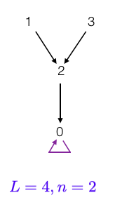
Figure 2. The Zolotarev graph $Z(2,4)$ has $2$ leaves, $1$ branch, and $1$ root. $1$ and $3$ are leaves in $Z(2,4)$, which means that the Taylor series coefficients $a(1)$ and $a(3)$ represent free variables. On the other hand, a sufficient and necessary condition for $f\in\ker(U_{2})$ is that $a(0)=a(2)=0$ (the roots and branches in $Z(2,4)$). Therefore, it is clear that $dim(\ker(U_{2}))=2$.

$\square$

Corollary 12.

Let $U_{n}:\mathcal{R}(L,\kappa)\rightarrow\mathcal{R}(L,\kappa).$ Then,

$$dim(ker(U_{n}))=L-\frac{L}{(n,L)}.$$

$\square$ (Proof)

The following result gives equivalences for diagonalizability.

Theorem 15.

The following conditions are equivalent:

1. $U_{n}:\mathcal{R}(L,\kappa)\rightarrow\mathcal{R}(L,\kappa)$ is diagonalizable.

2. $\frac{L}{(L,n)}=L_{n}$

3. $Z(n,L)$ has no branches.

4. $n$ is a root in $Z(n,L)$

5. $H(1)=1$

(Proof) $\square$

7. Proofs of section 1 Introduction

7.1. Proof of Theorem 1 and Lemma 1

Proof.

(of Theorem 1) By [12], Chapter 4, we may write the Taylor series coefficients of any function $f\in\mathcal{R}$ as

$$a(k)=\sum_{j=1}^{d}P_{j}(k)r_{j}^{k},$$

where degree $(P_{j}(k))=m_{j}-1$, $m_{j}$ is the multiplicity of each distinct pole $\frac{1}{r_{j}}$ of $f$ and $d$ is the number of poles of $f$. Therefore the Taylor series coefficients of $U_{n}(f)$ are

$$a(kn)=\sum_{j=1}^{d}P_{j}(kn)r_{j}^{kn}=\sum_{j=1}^{d}P_{j}(kn)(r_{j}^{n})^{k},$$

which shows that the poles of $U_{n}(f)$ are precisely $\left\{\frac{1}{r_{1}^{n}},\frac{1}{r_{2}^{n}},\dots,\frac{1}{r_{d}^{n}}\right\}$. On the other hand, our assumption that $U_{n}(f)=\lambda f$ implies that the rational functions $f$ and $U_{n}(f)$ have the same set of poles, namely $\left\{\frac{1}{r_{1}},\dots,\frac{1}{r_{d}}\right\}$. We now have:

(27) $$\left\{\frac{1}{r_{1}},\frac{1}{r_{2}},\cdots,\frac{1}{r_{d}}\right\}=\left\{\frac{1}{r_{1}^{n}},\frac{1}{r_{2}^{n}},\cdots,\frac{1}{r_{d}^{n}}\right\},$$

implying that the latter two sets must be permutations of each other. Considering the orbit of the pole $\frac{1}{r_{i}}$ under $U_{n}$, we know that the subset of poles of $f$ defined by $\left\{\frac{1}{r_{i}},\frac{1}{r_{i}^{n}},\frac{1}{r_{i}^{n^{2}}},\dots\right\}$ must be a finite set, so that for some integers $j,k$, we have $\frac{1}{r_{i}}^{n^{j}}=\frac{1}{r_{i}}^{n^{k}}$. Therefore $\frac{1}{r_{i}}^{n^{j}-n^{k}}=1$, so that $\frac{1}{r_{i}}$ is a root of unity and then also $r_{i}$ is a root of unity. ∎

Proof.

(of Lemma 1) The Taylor series coefficients of any function $f\in\mathcal{R}$ are given by [12]

$$a(k)=\sum_{j=1}^{d}P_{j}(k)r_{j}^{k},$$

where degree$(P_{j}(k))=m_{j}-1$, $m_{j}$ is the multiplicity of each distinct pole $\frac{1}{r_{j}}$ of $f$ and $d$ is the number of poles of $f$. If $f$ is an eigenfunction of $U_{n}$, with level $L$, then we know by Theorem 1 that all of its poles $\frac{1}{r_{j}}$, (and thus $r_{j}$) are $L$’th roots of unity. Indeed, there is a smallest integer $L$ with this property. Therefore:

$$a(k)=\sum_{j=1}^{d}P_{i}(k)e^{\frac{2\pi il_{j}k}{L}},$$

for some integers $l_{j}$.

Now we suppose to the contrary that $\gcd(n,L)=M>1$, so we have $n=n_{0}\cdot M,L=L_{0}\cdot M$, for some integers $n_{0}<n,L_{0}<L$. The action of $U_{n}$ on $f$ gives us the relation:

(28) $$a(k)\lambda=a(kn)=\sum_{j=1}^{d}P_{i}(nk)e^{\frac{2\pi il_{j}kn}{L}}=\sum_{j=1}^{d}P_{i}(k)e^{\frac{2\pi il_{j}kn_{0}}{L_{0}}},$$

implying that the poles of $f$ are all $L_{0}$´roots of unity, with $L_{0}<L$, a contradiction. ∎

7.2. Proof of Theorem 2, Theorem 3 and Corollary 1

.

Here, we’ll prove Theorem 2, Theorem 3 and Corollary 1 simultaneously.

Proof.

We may write the Taylor series coefficients of any function $f\in\mathcal{R}$ as

$$b(k)=\sum_{j=1}^{d}P_{j}(k)r_{j}^{k},$$

where degree$\left(P_{j}(k)\right)=m_{j}-1$ and $m_{j}$ is the multiplicity of each distinct pole $\frac{1}{r_{j}}$ of $f$. By assumption, we have

$$U_{n}(f)=\sum_{k=0}^{\infty}b(nk)x^{k}=\lambda\sum_{k=0}^{\infty}b(k)x^{k}.$$

Then, for all $k\in\mathbb{Z}_{\geq 0}$,

(29) $$b(nk)=\lambda b(k)$$

Let $L=\rm{level}(f)$. By Theorem 1, for all $i=1,2,\dots,d$, we have $r_{i}^{L}=1$. Also by Lemma 1, $(n,L)=1$, hence we can define $c:={\rm ord}_{L}(n)$. Now, iterating $U_{n}$ $c$ times to $f$, we have

$$b(kn^{c})=\sum_{j=1}^{d}P_{j}(kn^{c})r_{j}^{kn^{c}}=\lambda^{c}\sum_{j=1}^{d}P_{j}(k)(r_{j})^{k}.$$

On the other hand, $n^{c}\equiv 1\mod L$. Therefore, we have

$$\sum_{j=1}^{d}P_{j}(kn^{c})\left(r_{j}^{n^{c}}\right)^{k}=\sum_{j=1}^{d}P_{j}(kn^{c})r_{j}^{k}=\lambda^{c}\sum_{j=1}^{d}P_{j}(k)(r_{j})^{k}.$$

By uniqueness of the finite Fourier series, for all $j=1,2,\dots,d$

(30) $$P_{j}(kn^{c})=\lambda^{c}P_{j}(k).$$

Now, because (30) holds for every integer $k$, we have that the coefficients of both polynomials are indeed equal. Let $P_{j}(k)=\sum_{i=0}^{m_{j}-1}a_{i,j}k^{i}.$ The latter observation can be expressed by the following system:

$$\begin{cases}a_{0,j}=\lambda^{c}a_{0,j}\\ a_{1,j}n^{c}=\lambda^{c}a_{1,j}\\ \vdots\\ a_{i,j}n^{ic}=\lambda^{c}a_{i,j}\\ \vdots\\ a_{m_{j}-1,j}n^{(m_{j}-1)c}=\lambda^{c}a_{m_{j}-1,j}\end{cases}$$

Note that $a_{m_{j}-1,j}\neq 0$, because degree$(P_{j}(k))=m_{j}-1$. Thus, $n^{(m_{j}-1)c}=\lambda^{c}$

But, because $n>1$, $\lambda^{c}\neq n^{ic}$, for all $i\neq m_{j}-1$, and, therefore, $a_{i,j}=0$. Indeed,

(31) $$b(k)=\sum_{j=1}^{d}P_{j}(k)r_{j}^{k}=\sum_{j=1}^{d}C_{j}k^{m_{j}-1}r_{j}^{k},$$

where $C_{j}=a_{m_{j}-1,j}$.

Finally, from the equality $n^{(m_{j}-1)c}=\lambda^{c}$, which holds for all $j=1,2,\dots,d$, and from the fact that $\lambda$ is a constant independent of $j$, we conclude that $\kappa:=m_{1}=m_{2}=\dots=m_{d}$, proving Theorem 2. Moreover, for some $c$’th root of unity $\omega$,

$$\lambda=\omega n^{\kappa-1},$$

which concludes the proof of Theorem 3.

Now, returning to the series expansion (31), we replace all the multiplicities $m_{j}$ by $\kappa$, getting

$$b(k)=\sum_{j=0}^{d}k^{\kappa-1}C_{j}r_{j}^{k}=k^{\kappa-1}\sum_{j=0}^{d}C_{j}r_{j}^{k}.$$

Let $a(k)=\frac{b(k)}{k^{\kappa-1}}$. It follows from Theorem 1 that $a(k+L)=a(k)$, because

(32) $$a(k+L)=\sum_{j=0}^{d}C_{j}r_{j}^{k+L}=\sum_{j=0}^{d}C_{j}r_{j}^{k}r_{j}^{L}=\sum_{j=0}^{d}C_{j}r_{j}^{k}=a(k).$$

Moreover, suppose there exists an integer $M<L$ such that $a(k+M)=a(k)$ for all $k$, i.e.

$$a(k+M)=\sum_{j=0}^{d}C_{j}r_{j}^{k+M}=\sum_{j=0}^{d}\left(C_{j}r_{j}^{M}\right)r_{j}^{k}=\sum_{j=0}^{d}C_{j}r_{j}^{k}=a(k)$$

Then, by the uniqueness of the finite Fourier series, all the coefficients must be equal. In particular, for $k=0$,

$$C_{j}r_{j}^{M}=C_{j}\Rightarrow r_{j}^{M}=1\,\forall j,$$

a contradiction, as this would imply that the level of $f$ is $M\not=L$, and therefore concluding the proof of Corollary 1. ∎

7.3. Proof of Corollary 2

Proof.

(of Corollary 2) We define:

(33) $$\mathfrak{A}_{n}:=\{\lambda(m,L,\kappa):=e^{\frac{2\pi im}{c}}n^{\kappa-1}\mid m\in\mathbb{Z},\ \kappa,L\text{ are positive integers},\text{ and }(n,L)=1\},$$

where $c:={\rm ord}_{L}(n)$. Then by Theorem 3 and Lemma 1, we know that $\rm{Spec}\left(U_{n}\right)\subseteq\mathfrak{A}_{n}$.

To prove that $\mathfrak{A}_{n}\subseteq\rm{Spec}\left(U_{n}\right)$, it remains to show that for each $m\in\mathbb{Z}$, and $\kappa,L$ positive integers with $(n,L)=1$, there exists a function $f$ that satisfies $U_{n}(f)=\lambda(m,L,\kappa)f$. Fix $\rm{level}(f)=L$ and $\rm{weight}(f)=\kappa$. Then, by Corollary 1, we have

$$f(x)=\sum_{k=0}^{\infty}k^{\kappa-1}a(k)x^{k}.$$

We fix $a(1)=1$ and $\omega:=e^{\frac{2\pi im}{c}}$. We define:

$$a(k):=\begin{cases}\omega^{v},&\text{ if there exists an integer }v\ \left(\mathrm{mod}\ c\right)\text{ such that }k\equiv n^{v}\ \left(\mathrm{mod}\ L\right),\\ 0,&\text{ otherwise.}\end{cases}$$

We first show that $a(k)$ is well defined. Suppose we have two integers $v_{1},v_{2}$ that satisfy the latter property. If $v_{1}\equiv v_{2}\ \left(\mathrm{mod}\ c\right)$, then $a(k)=\omega^{v_{1}}=\omega^{v_{2}}$, because $\omega$ is a $c$’th root of unity. Now we apply $U_{n}$ to $f$:

$$U_{n}(f(x))=\sum_{k=0}^{\infty}(nk)^{\kappa-1}a(nk)x^{k}.$$

If $k\equiv n^{v}\ \left(\mathrm{mod}\ L\right)$, then $nk\equiv n^{v+1}\ \left(\mathrm{mod}\ L\right)$, thus $a(nk)=\omega^{v+1}=\omega a(k)$. On the other hand, if such an integer $v$ does not exists for $k$, then it does not exist for $nk$. Therefore $a(nk)=0=\omega a(k)$. Therefore,

$$U_{n}(f(x))=\sum_{k=0}^{\infty}n^{\kappa-1}k^{\kappa-1}\omega a(k)x^{k}=\omega n^{\kappa-1}f(x)$$

Thus, for each triplet $(m,L,\kappa)$, there exists an eigenfunction $f$ of $U_{n}$, with eigenvalue $\lambda(m,L,\kappa)$. Therefore, we conclude that $\mathfrak{A}_{n}\subseteq\rm{Spec}\left(U_{n}\right)$. ∎

7.4. Proof of Corollary 3

Proof.

(of Corollary 3) Let $x\in\mathbb{Z}_{>0}$ be such that $\phi(x)=N$. By Dirichlet´s theorem on primes in arithmetic progressions, there exists a prime $p$ such that $p\equiv 1\pmod{N}$, i.e., there exists $j\in\mathbb{Z}_{>0}$ such that $N\cdot j=p-1=\phi(p).$ Let $g$ be a primitive root modulo $p$. We now have ${\rm ord}_{p}(g^{j})=N$. Therefore, by Corollary 2, $e^{\frac{2\pi i}{N}}\in\text{Spec}(U_{n})$. ∎

7.5. Proof of Lemma 2

Proof.

(of Lemma 2) We will prove that $\mathcal{R}(L,\kappa)$ is a finite subspace of the infinite dimensional vector space $\mathcal{R}$. It is clear that $\mathcal{R}(L,\kappa)\subset\mathcal{R}$. Note also that the null function $0(x)=0,\forall x\in\mathbb{C}$ lies in $\mathcal{R}(L,\kappa)$, for all $L$ and $\kappa$. Indeed, $0=\sum_{k=0}^{\infty}k^{\kappa-1}a(k)x^{k}$, where $a(k)=0$ for every $k$, thus $0\in\mathcal{R}(L,\kappa)$. Now, we prove that $\mathcal{R}(L,\kappa)$ is closed over sum and multiplication by scalar: For every $f,g\in\mathcal{R}(L,\kappa)$, we have

$$(f+g)(x)=\sum_{k=0}^{\infty}k^{\kappa-1}a(k)x^{k}+\sum_{k=0}^{\infty}k^{\kappa-1}b(k)x^{k}=\sum_{k=0}^{\infty}k^{\kappa-1}(a+b)(k)x^{k}.$$

Note that $(a+b)(k+L)=a(k+L)+b(k+L)=a(k)+b(k)=(a+b)(k)$, i.e., $f+g\in\mathcal{R}(L,\kappa)$. Also, for every $\alpha\in\mathbb{C}$, we have

$$\alpha\cdot f=\sum_{k=0}^{\infty}k^{\kappa-1}(\alpha\cdot a)(k)x^{k}.$$

Note that $(\alpha\cdot a)(k+L)=\alpha\cdot a(k+L)=(\alpha\cdot a)(k)$, thus $\alpha f\in\mathcal{R}(L,\kappa)$, proving that $\mathcal{R}(L,\kappa)$ is a subspace of $\mathcal{R}$.

It is easy to see that $\dim\mathcal{R}(L,\kappa)=L$. Indeed, as defined in (6), the indicator function $1_{a\text{ mod }L}(k)$ of the congruence class $\{n\in\mathbb{Z}\mid n\equiv a\mod L\}$ is the natural basis for the space of all periodic functions with period $L$. In particular, by Corollary 1, the Taylor series coefficients $a(k)$ have period $L$. Thus, we have that

$$\left\{\sum_{k=0}^{\infty}k^{\kappa-1}1_{a\text{ mod }L}(k)x^{k}=\sum_{k=0}^{\infty}(a+kL)^{\kappa-1}x^{(a+kL)}\mid 0\leq a<L\right\}$$

is a basis of $\mathcal{R}(L,\kappa)$, which proves that $\dim\mathcal{R}(L,\kappa)=L$. ∎

7.6. Proofs of Lemma 3 and Lemma 4

Proof.

(of Lemma 3) For clarity, we first prove the formula for the number of fixed points of $\tau(n,L)$, namely we must show that $b_{1}=\gcd(n-1,L)$, as predicted by formula (10). Suppose that some $k\mod L$ forms a cycle of length $1$, in the permutation $\tau(n,L)$. This means that $nk\equiv k\mod L$. The latter congruence is equivalent to $L\mid k(n-1)$, which in turn is equivalent to $\frac{L}{\gcd(L,n-1)}\mid k$. Now it’s easy to count how many integers $0\leq k<L$ are multiples of $\frac{L}{\gcd(L,n-1)}$: there are exactly $\gcd(L,n-1)$ of them, including $0$. This proves formula (10) for $j=1$.

Now we extend the argument above, to prove the required formula (10) for all $b_{j}$. Suppose we have a cycle of length less than or equal to $j$: $(k,\overline{nk},\dots,\overline{n^{j-1}k})$, which means that

$$n^{j}k\equiv k\mod L,$$

and it is elementary that the latter congruence is equivalent to

$$\frac{L}{\gcd(n^{j}-1,L)}\mid k.$$

The same divisibility criterion also holds for each of the elements in the same cycle. Therefore, counting the total number of cycles of length $\leq j$, we have:

$$\sum_{d\mid j}db_{d}=\gcd(n^{j}-1,L).$$

Applying Möbius inversion, we arrive at:

$$jb_{j} =\sum_{d\mid j}\mu\left(\frac{j}{d}\right)\gcd(n^{d}-1,L).$$

∎

Proof.

(of Lemma 4)

1. Suppose there exists $k\nmid c={\rm ord}_{L}(n)$ such that $k$ is the size of a cycle that $n$ creates in $\mathbb{Z}/L\mathbb{Z}$, $i.e.$, there exists an integer $m$ such that

   $$m\cdot n^{k}\equiv m\pmod{L}.$$

   Multiplying the two sides by $n^{c-k}$, we have

   $$m\cdot n^{c}\equiv m\cdot n^{c-k}\pmod{L}.$$

   Now, we use $n^{c}\equiv 1\pmod{L}$, getting

   $$m\equiv m\cdot n^{c-k}\pmod{L}.$$

   Then, by definition, $k$ is the smallest integer $a$ such that $m\equiv m\cdot n^{a}\pmod{L}$. Thus, $c-k>k$, i.e., $k<\frac{c}{2}$.

   Now we can take $c-k\equiv b\pmod{k}$, where $0<b<k$, since $k\nmid c$. But, therefore

   $$m\equiv m\cdot n^{b}\pmod{L},$$

   a contradiction.
   

2. It’s clear that if $A\cap B=\varnothing$, then $A\not=B$, since $A\not=\varnothing$.

   Now we prove the converse. Let $A=\left\{a\cdot n^{i}\in\mathbb{Z}/L\mathbb{Z}\mid i\in\mathbb{Z}\right\}$ and $B=\left\{b\cdot n^{i}\in\mathbb{Z}/L\mathbb{Z}\mid i\in\mathbb{Z}\right\}$. Suppose there exist $i$ and $j$ such that $a\cdot n^{i}\equiv b\cdot n^{j}\pmod{L}$, i.e., $A\cap B\not=\varnothing$. We will show that the sets A and B are, in fact, equal.

   For all $m\in\mathbb{Z}$, we have $a\cdot n^{i+m}\equiv b\cdot n^{j+m}\pmod{L}$. We therefore create the cycle $A=\left\{a\cdot n^{i+m}\in\mathbb{Z}/L\mathbb{Z}\mid m\in\mathbb{Z}\right\}=\left\{b\cdot n^{j+m}\in\mathbb{Z}/L\mathbb{Z}\mid m\in\mathbb{Z}\right\}=B$.
   

3. The latter proof not only shows that all different cycles are disjoint, but also proves that if $b_{j}$ is the number of different cycles of size $j$, then $\sum_{j=1}^{c}jb_{j}=L$, concluding the proof of the Lemma.

∎

8. Proofs of section 2, Zolotarev Graphs

8.1. Proof of Lemma 5

Proof.

(of Lemma 5) Let $c$ be one of the $(n,L)$ solutions to $n\cdot c\equiv k\mod L$. Writing any other integer as $c+m$, we have that $n\cdot(c+m)=n\cdot c+n\cdot m\equiv k+n\cdot m\mod L$. But,

$$k+n\cdot m\equiv k\ \left(\mathrm{mod}\ L\right)\iff n\cdot m\equiv 0\ \left(\mathrm{mod}\ L\right)\iff\exists b\in\mathbb{Z}\text{ such that }n\cdot m=b\cdot L.$$

Let $n=d\cdot(n,L)$, with $(d,L)=1.$ Then,

$$m=b\cdot\frac{L}{d(n,L)}=\frac{b}{d}\cdot\frac{L}{(n,L)}.$$

But, because $(d,L)=1$, we have

$$\frac{b}{d}\cdot\frac{L}{(n,L)}\in\mathbb{Z}\implies\frac{b}{d}\in\mathbb{Z}.$$

Thus, $m$ is another solution to $n\cdot c\equiv k\pmod{L}$ if, and only if, $m=c+j\frac{L}{(n,L)}$. Therefore, all $(n,L)$ solutions are congruent modulo $\frac{L}{(n,L)}.$ ∎

8.2. Proofs of Theorem 4, Corollary 4 and Lemma 6

Proof.

(of Theorem 4)

1. Let $m\in Z(n,L)$ and suppose $(n,L)\mid m$. Then, there exists an integer $k$ such that
   $m\equiv n\cdot k\ \left(\mathrm{mod}\ L\right)$. Thus, by definition $m$ is not a leaf. The converse is analogous.

2. Suppose $\frac{L}{L_{n}}\nmid m$. Note that $\frac{L}{L_{n}}$ is exactly the product of the powers of primes that divide $L$ and appear in the factorization of $n$ (with eventually different exponents). Thus, there exists an integer $k$´ such that $\frac{L}{L_{n}}\mid m\cdot n^{k^{\prime}}$. Then, by definition, $m$ is not a root.

   Conversely, suppose $m=k\cdot\frac{L}{L_{n}}$, for some integer $k$. Indeed, there exists an integer $j$ such that

   (34) $$n\cdot m=n\cdot k\cdot\frac{L}{L_{n}}\equiv j\cdot\frac{L}{L_{n}}\ \left(\mathrm{mod}\ L\right).$$

   Dividing by $\frac{L}{L_{n}}$,

   (35) $$n\cdot k\equiv j\ \left(\mathrm{mod}\ L_{n}\right).$$

   Now, because $(n,L_{n})=1$, there exists a positive exponent $l$ such that

   $$n^{l}\cdot k\equiv k\ \left(\mathrm{mod}\ L_{n}\right)\implies n^{l}\cdot m\equiv m\ \left(\mathrm{mod}\ L\right),$$

   i.e., $m$ is a root in $Z(n,L)$, concluding the proof of (b).

3. follows trivially from the latter two items and the definition of branch.

∎

Proof.

(of Corollary 4)

1. Note that $|\{m\in\left(\mathbb{Z}/L\mathbb{Z}\right)\mid m=k\cdot\frac{L}{L_{n}}\}|=|\{k\mid 0\leq k<L_{n}\}|=L_{n}$. Therefore, by Theorem 4, we have $L_{n}$ roots.

2. Note that $|\{m\in\left(\mathbb{Z}/L\mathbb{Z}\right)\mid m=k\cdot(n,L)\}|=|\{k\mid 0\leq k<\frac{L}{(n,L)}\}|=\frac{L}{(n,L)}$. Then, by Theorem 4, we have $\frac{L}{(n,L)}$ nodes which are not leaves, impliying that $|\text{roots}|=L-\frac{L}{(n,L)}$, and $|\text{branches}|=\frac{L}{(n,L)}-L_{n}$.

3. Let $F:=|\text{leaves}|$. By Lemma 5, the indegree of all nodes which are not leaves is $(n,L)$. Thus, there are exactly $(n,L)\cdot(L-F)$ edges in $Z(n,L)$. On the other hand, there are $L$ nodes, an therefore $L$ edges in total. Therefore, we have

   $$(n,L)\cdot(L-F)=L\iff F=L\cdot\frac{(n,L)-1}{(n,L)}$$

∎

Proof.

(of Lemma 6) By Theorem 4, a node $r$ in $Z(n,L)$ is a root if, and only if, $\frac{L}{L_{n}}\mid r$. Then,

$$\frac{L}{L_{n}}\mid k\cdot L_{n}\iff k\equiv 0\ \left(\mathrm{mod}\ \frac{L}{L_{n}}\right),$$

because $\left(\frac{L}{L_{n}},L_{n}\right)=1$. Note that for each root $r$, we can construct a set of size $\frac{L}{L_{n}}$ given by $\{r+k\cdot L_{n}\mid 0\leq k<\frac{L}{L_{n}}\}$. Moreover, the sets are disjoint, because, by construction, each set contains only one root. Thus, we partitioned $Z(n,L)$ in $L_{n}$ sets. ∎

8.3. Proofs of Theorem 5, Theorem 6 and Theorem 7

Proof.

(of Theorem 5) Note that $m$ is a root if, and only if, $m$ is in a cycle in $Z(n,L)$. Hence, there are exactly $j\cdot b_{j}$ roots, where $b_{j}$ is number of cycles in $Z(n,L)$ of size $j$. It is clear that for any $j>L$, we have $b_{j}=0$. Therefore, by Observation 1, the number of roots is given by:

$$|\text{roots}|=\sum_{j=1}^{L}j\cdot b_{j}=\sum_{j=1}^{L}\sum_{d\mid j}\mu\left(\frac{j}{d}\right)\text{gcd}(n^{d}-1,L).$$

∎

Proof.

(of Theorem 6) It is easy to see that there exists an integer $k$ such that $n^{k}m\equiv 0\mod L$ if, and only if, $L_{n}\mid m$. Also, $n^{d(L_{n},0)}\cdot k\cdot L_{n}\equiv k\cdot 0\equiv 0\mod L$, which implies $d(L_{n},0)\geq d(kL_{n},0)$ for any integer $k$.

∎

Proof.

(of Theorem 7) Let $a$ and $b$ be two nodes, $i$ a root in the same connected component as $a$ and $b$ and suppose $a\equiv b\ \left(\mathrm{mod}\ L_{n}\right)$. Let $b=a+kL_{n}$. By Theorem 6, for every node $kL_{n}\in\rm{Tree}(0)$, there exists an integer $\beta$ such that $n^{\beta}\cdot kL_{n}\equiv 0\ \left(\mathrm{mod}\ L\right)$. We have

$$n^{d(b,i)}\cdot b=n^{d(a+kL_{n},i)}\cdot(a+kL_{n})\equiv i\ \left(\mathrm{mod}\ L\right).$$

Thus, there exists an integer $\alpha$ such that $d(b,i)+\alpha j>\beta$. Therefore, we obtain the following:

$$n^{d(a+kL_{n},i)+\alpha j}\cdot(a+kL_{n})=n^{d(a+kL_{n},i)+\alpha j}\cdot a+n^{d(a+kL_{n},i)+\alpha j}\cdot kL_{n}\equiv n^{d(a+kL_{n},i)+\alpha j}\cdot a\equiv i\ \left(\mathrm{mod}\ L\right)$$

Then, for any integer $k$, the following holds:

$$d(a+kL_{n},i)+\alpha j\equiv d(a+kL_{n},i)\equiv d(a,i)\ \left(\mathrm{mod}\ j\right)$$

Conversely, let $i$ be a root in a cycle of size $j$ and $a$ and $b$ two nodes in the same connected component as $i$ such that $d(a,i)\equiv d(b,i)\ \left(\mathrm{mod}\ j\right)$. Let $\gamma:=b-a$ and $\alpha$ an integer such that $d(b,i)=d(a,i)+\alpha\cdot j$. Then, we have the following:

$$i\equiv n^{d(b,i)}\cdot b=n^{d(b,i)}\cdot a+n^{d(b,i)}\cdot\gamma=n^{d(a,i)+\alpha j}\cdot a+n^{d(b,i)}\cdot\gamma\equiv i+n^{d(b,i)}\cdot\gamma\ \left(\mathrm{mod}\ L\right).$$

Therefore, we conclude that $n^{d(b,i)}\cdot\gamma\equiv 0\ \left(\mathrm{mod}\ L\right)$ and, by Theorem 6, $\gamma$ is a multiple of $L_{n}$, hence $a\equiv b\ \left(\mathrm{mod}\ L_{n}\right)$. ∎

8.4. Proof of Lemma 7

Proof.

(of Lemma 7) Let $i$ be the root such that $n^{H(1)}\equiv i\ \left(\mathrm{mod}\ L\right)$ and $k\in Z(n,L)$ be any node. We have

$$n^{H(1)}\cdot 1 \equiv i\ \left(\mathrm{mod}\ L\right)$$

$$n^{H(1)}\cdot k \equiv i\cdot k\ \left(\mathrm{mod}\ L\right)$$

$$\implies H(k)\leq H(1),$$

because $k\cdot i$ is a root in $Z(n,L)$. ∎

8.5. Proof of Theorem 8

Proof.

(of Theorem 8) Let $g:=$gcd$(n,L)$ and suppose $Z(n,L)$ has homogeneous height $h$, i.e., all its leaves have the same height $h$. By Lemma 5, if $r$ is a root in $Z(n,L)$, its indegree is $g$, from which $g-1$ edges connect $r$ to leaves and branches. Thus, there are $L_{n}\cdot(g-1)$ nodes $m$ with $H(m)=1$. Note that if $m$ is a branch, then its indegree is $g$. Therefore, we conclude, inductively, that, for every $i\leq h$, we have $|\{m\mid H(m)=i\}|=L_{n}\cdot(g-1)\cdot g^{i-1}$.

As there are $L$ nodes in total, we have the following:

$$L=L_{n}+\sum_{m=1}^{h}L_{n}(g-1)g^{m-1}=L_{n}\left(1+(g-1)\sum_{m=0}^{h-1}g^{m}\right)$$

$$=L_{n}\left(1+(g-1)\cdot\frac{g^{h}-1}{g-1}\right)=L_{n}\cdot g^{h}$$

$$\iff L_{n}=\frac{L}{g^{h}}.$$

Conversely, suppose $L_{n}=\frac{L}{g^{h}}$. Let $L=\prod_{i=1}^{s}p_{i}^{\alpha_{i}}$, $n=\prod_{i=1}^{t}q_{i}^{\beta_{i}}$ and $\{r_{i}\mid 1\leq i\leq max\{s,t\}\}$ be the set of primes shared by $L$ and $n$. Then, $\alpha_{i}=c\cdot\beta_{i}$, for some integer $c$.

Claim: If $m$ is a leaf in $Z(n,L)$, then $H(m)=c$.

Indeed, by Theorem 4, if $m$ is a leaf, then $g\nmid m$, i.e., gcd$(g,m)=\prod r_{i}^{\gamma_{i}}$. Moreover, there exists an integer $i^{\prime}$ such that $\gamma_{i^{\prime}}<\beta_{i^{\prime}}$. But, by Theorem 4 $n^{k}m$ is a root if, and only if, $\frac{L}{L_{n}}=g^{h}\mid n^{k}m$, i.e., for all $i$, $\gamma_{i}+k\cdot\beta_{i}\geq h\cdot\beta_{i}$. But, because $\gamma_{i^{\prime}}<\beta_{i^{\prime}}$, we have $\gamma_{i^{\prime}}+k\cdot\beta_{i^{\prime}}\geq h\cdot\beta_{i^{\prime}}\iff k\geq h$, which implies $H(m)=h$, concluding the proof. ∎

8.6. Proof of Theorem 9, Corollary 5, Corollary 6 and Corollary 7

Proof.

(of Theorem 9) The idea of the proof is the well-known identity:

(36) $$a\equiv b\ \left(\mathrm{mod}\ c\right)\iff\frac{a}{d}\equiv\frac{b}{d}\ \left(\mathrm{mod}\ \frac{c}{d}\right),$$

where $d$ is any common divisor of $a,b,c$. Consider the function $\psi:G\rightarrow Z(n,\frac{L}{v})$, defined by:

$$\psi(x)=\frac{x}{v}.$$

Note that

$$\psi(x)\equiv\psi(y)\ \left(\mathrm{mod}\ \frac{L}{v}\right)\iff\frac{x}{v}\equiv\frac{y}{v}\ \left(\mathrm{mod}\ \frac{L}{v}\right)\iff x\equiv y\ \left(\mathrm{mod}\ L\right),$$

by (36). Hence, $\psi$ is injective. Also, because the two graphs have $\frac{L}{v}$ nodes, we conclude that $\psi$ is a bijection. Moreover, $\psi$ has the isomorphism property (17): If $a\longmapsto b\equiv na\mod L$, then by (36),

$$\psi(b)=\frac{b}{v}\equiv\frac{na}{v}=n\psi(a)\ \left(\mathrm{mod}\ \frac{L}{v}\right)\iff\psi(a)\longmapsto\psi(b),$$

concluding the proof. ∎

Proof.

(of Corollary 5) By Theorem 6, $x\in{\rm Tree}(0)\iff L_{n}\mid x$. Thus, by Theorem 9 the proof is done. ∎

Proof.

(of Corollary 6) By Theorem 4, all the non-leaves are multiples of $(n,L)$. Thus, it is a particular case of Theorem 9. ∎

Proof.

(of Corollary 7) Apply Theorem 9 with $v=\frac{L}{L_{n}}.$ ∎

9. Proofs of section 3: The eigenspaces

9.1. Proofs of Theorem 10, Corollary 8 and Theorem 11

Proof.

(of Theorem 10) First, we will show that $F_{\omega,L,\kappa,n,r}\in E_{n}(\omega,L,\kappa).$

Indeed, if $i\neq r$ is connected to $r$, then $d(ni,r)=d(i,r)-1$. Thus,

(37) $$a_{\omega,L,n,r}(ni)=\omega^{-d(ni,r)}=\omega^{-d(i,r)+1}=\omega a_{\omega,L,n,r}(i).$$

If $i=r$, because the cycle has size $jm$ and $\omega$ is a $m$’th root of unity, we have

(38) $$a_{\omega,L,n,r}(nr)=\omega^{-d(ni,r)}=\omega^{-bm+1}=\omega=\omega a_{\omega,L,n,r}(r).$$

If $i$ is not connected to $r$, then neither is $ni$, and therefore $a_{\omega,L,n,r}(ni)=\omega a_{\omega,L,n,r}(i)=0$.

If $r$ and $k$ share a cycle, $F_{\omega,L,\kappa,n,r}$ and $F_{\omega,L,\kappa,n,k}$ are linearly dependent, because $F_{\omega,L,\kappa,n,r}=\omega^{d(r,k)}F_{\omega,L,\kappa,n,k}$. But taking just one root $r_{i}$ from each disjoint cycle $A_{i}\in B_{m},1\leq i\leq|B_{m}|$ , we find that they are linearly independent, because

$$a_{\omega,L,n,r_{j}}(r_{i})=\begin{cases}1,&\text{ if $i=j$}\\ 0,&\text{ if $i\neq j$}\end{cases}$$

Then we can take in particular $\{F_{\omega,L,\kappa,n,r}\mid\ \ r=\min(A)\}$, implying that they are linearly independent

Now we show that they span the space. Let $f(x)=\sum_{k=0}^{\infty}k^{\kappa-1}a(k)x^{k}\in E_{n}(\omega,L,\kappa)$ and consider the Zolotarev graph $Z(n,L)$. By Corollary 1, we have $a(k)=a(k+L)$, for all $k\in\mathbb{Z}_{\geq 0}$ and $a(nk)=\omega a(k).$ If $k$ is a root in a cycle of size $j$, then $a(n^{j}k)=a(k)=\omega^{j}a(k)$ and, therefore, we have $a(k)=0$ or $\omega^{j}=1$. Indeed, if $\omega^{j}\neq 1$, then $a(k)=0$ and if $\omega^{j}=1$, we have $a(b)=a(k)\cdot a_{\omega,L,n,k}(b)$, for every node $b$ in the same connected component as $k$. Therefore,

$$f(x)=\sum_{\begin{subarray}{c}{r=min(A)}\\ {A\in B_{m}}\end{subarray}}a(r)\cdot F_{\omega,L,\kappa,n,r}(x),$$

concluding the proof.

∎

Proof.

(of Corollary 8) Let $f\in E_{n}(\omega,L,\kappa)$. We will show that $f\in E_{n}(\omega,L_{n},\kappa)$. Note that, by the definition of $E_{n}(\omega,L,\kappa)$, we have that $level(f)\mid L$. However, by Lemma 1, gcd$(level(f),n)=1$. Therefore, $level(f)\mid L_{n}$ and we conclude that $E_{n}(\omega,L,\kappa)\subset E_{n}(\omega,L_{n},\kappa)$.

On the other hand, note that $L_{n}\mid L\implies E_{n}(\omega,L_{n},\kappa)\subset E_{n}(\omega,L,\kappa)$, concluding the proof. ∎

Proof.

(of Theorem 11) It follows from Theorem 10 that $\dim E_{n}(\omega,L,\kappa)=|B_{m}|$, where $B_{m}$ is defined in (18). Indeed, $|B_{m}|$ is the sum of the number of cycles of size $j$ in $Z(n,L)$, where $m\mid j$. Therefore, we have the following:

$$|B_{m}|=\dim E_{n}(\omega,L,\kappa)=\sum_{m\mid j}^{L}b_{j}=\sum_{j=1}^{c}b_{mj}$$

∎

9.2. Proof of Theorem 12, Corollary 9 and Corollary 10

Proof.

(of Theorem 12) Let $A$ be a cycle of size $j$ in $Z(n,L)$, $r\in A$ and a $j$’th root of unity $\omega$. Accordingly, let $F_{\omega,L,\kappa,n,r}$ be a basic function of the non trivial eigenspace $E_{n}(\omega,L,\kappa)$. Note that the subspace spanned by $F_{\omega,L,\kappa,n,r}$ has dimension 1. Indeed, as there are $j$ $j$’th roots of unity, we have, for each cycle of size $j$, $j$ dimensions (one for each distinct root of unity). Thus, $\dim S_{n}(L,\kappa)$ is equal the number of roots in $Z(n,L)$. Indeed, by Corollary 4, we conclude that there are exactly $L_{n}$ roots and, therefore, $\dim S_{n}(L,\kappa)=L_{n}$, concluding the proof.

∎

Proof.

(of Corollary 9) By Corollary 8, we have that $E_{n}(\omega,L,\kappa)\subset\mathcal{R}(L_{n},\kappa)$, for every $\omega$. Thus, by definition, we conclude that $S_{n}(L,\kappa)\subset\mathcal{R}(L_{n},\kappa)$. Now, because of Theorem 12 and Lemma 2, $\dim S_{n}(L,\kappa)=\dim\mathcal{R}(L_{n},\kappa)$. Therefore, the two spaces are equal.

∎

Proof.

(of Corollary 10) By Theorem 12, $\dim S_{n}(L,\kappa)=L_{n}$. Therefore, it is sufficient to show that $g(n,L):=L_{n}$ is periodic in $n$ and completely multiplicative in $L$.

First, we show that $g$ is periodic in $n$. Note that

$$\gcd(n,L)=\gcd(n+L,L)\implies g(n,L)=g(n+L,L),$$

by the algorithm described in example (4).

Now, we show that $g$ is completely multiplicative in $L$. Let $A$, $B$ and $n$ be integers. Consider the trivial decomposition $A=\frac{A}{A_{n}}\cdot A_{n}$ and $B=\frac{B}{B_{n}}\cdot B_{n}.$ We have

$$A\cdot B=\frac{A\cdot B}{A_{n}\cdot B_{n}}\cdot A_{n}\cdot B_{n}.$$

Now, note that $(A_{n}\cdot B_{n})\mid A\cdot B$ and it is indeed the largest divisor of $A\cdot B$ which is coprime to $n$, because if $p$ is a prime such that $p\mid\frac{A\cdot B}{A_{n}\cdot B_{n}}$, then $p\mid\frac{A}{A_{n}}$ or $p\mid\frac{B}{B_{n}}$. In any case, $p\mid n$, and we are done. ∎

10. Proofs of section 4 Simultaneous eigenfunctions

10.1. Proofs of Lemma 8, and Corollary 11

Proof.

(of Lemma 8)

1. By Corollary 1:

   $$U_{n}\left(f(x)\right)=\sum_{k=0}^{\infty}(nk)^{\kappa-1}a(nk)x^{k}=n^{\kappa-1}\omega_{f}(n)\cdot f=\sum_{k=0}^{\infty}(nk)^{\kappa-1}\omega_{f}(n)a(k)x^{k}\Longleftrightarrow a(nk)=\omega_{f}(n)a(k),$$

   for all $k\geq 0$.

2. Let $f\in\mathcal{R}$. Then,

   $$U_{i}\circ U_{j}(f)=U_{i}(\sum_{k=0}^{\infty}a(j\cdot n)x^{k})=\sum_{k=0}^{\infty}a(i\cdot j\cdot k)x^{k}=U_{i\cdot j}.$$

   Thus, $U_{i}\circ U_{j}=U_{i\cdot j}$. Therefore, $U_{n}\circ U_{m}(f)=U_{n}(\omega_{f}(m)f)=\omega_{f}(n)\omega_{f}(m)f=U_{mn}(f)$, implying $mn\in\mathcal{C}(f)$ and $\omega_{f}(m\cdot n)=\omega_{f}(m)\cdot\omega_{f}(n)$.

3. Let $f\in E_{m}(\omega_{f}(m),L,\kappa)$. By Lemma 1, $a(k+L)=a(k)$ for all $k\geq 0$. Applying the operator $U_{m+L}$, we have:

   $$U_{m+L}\left(f(x)\right) =\sum_{k=0}^{\infty}((m+L)k)^{\kappa-1}a((m+L)k)x^{k}$$

   $$=\left(m+L\right)^{\kappa-1}\sum_{k=0}^{\infty}(k)^{\kappa-1}a(mk)x^{k}$$

   $$=\left(m+L\right)^{\kappa-1}\omega_{f}(m)\sum_{k=0}^{\infty}(k)^{\kappa-1}a(k)x^{k},$$

   which implies $m+L\in\mathcal{C}(f)$ and $\omega_{f}(m+L)=\omega_{f}(m)$.

4. By the latter two proofs, we easily conclude that $\omega_{f}$ is a completely multiplicative and periodic function, with period $L$. Moreover, by Lemma 1, if $\left(d,L\right)>1$ and $d\in\mathcal{C}(f)$, implying $\omega_{f}(d)=0$. Therefore, there exists a Dirichlet character modulo L $\chi$ such that $\omega_{f}=\chi|_{\mathcal{C}(f)}$ concluding the proof of the Lemma.

∎

Proof.

(of Corollary 11) If Level$(f)=\overline{L}$, then, by Lemma 8, there exists a Dirichlet character modulo $\overline{L}$ such that $\chi(n)=\omega_{f}(n)$, for all $n\in\mathcal{C}(f)$. In particular, for $\mathcal{C}(f)=\mathbb{Z}$, the result follows. ∎

Proof.

(of Lemma 9) Suppose $p\mid c$ and that there exists $k\in\mathbb{Z}$ with $\left(M+k\cdot c,L\right)>1$. Then, there exists a prime $q$ such that $q\mid L$ and $q\mid M+k\cdot c$. As $L=p\cdot c$, we have $q\mid p$ or $q\mid c$. But $q\mid p\mid c$, then $q\mid c$. Therefore:

$$\begin{cases}q\mid c\\ q\mid M+k\cdot c\end{cases}\Rightarrow q\mid M,$$

contradicting $(M,L)=1$.

Conversely, assume that for all $k\in\mathbb{Z}$, $(M+kc,L)=1$. Suppose that $p\nmid c$. Then, there exists is a prime $q$ such that $q\mid p$ and $q\nmid c$. But $p\mid L\implies q\mid L$, and $(M,L)=1\implies q\nmid M$.

Now, if $(M+kc,L)=1$, then $q\nmid M+kc$. Let $\overline{M}$ and $\overline{q}$ be such that $M\equiv\overline{M}\ \left(\mathrm{mod}\ q\right)$ and $c\equiv\overline{c}\ \left(\mathrm{mod}\ q\right)$. However, $\left(\mathbb{Z}/q\mathbb{Z}\right)^{*}$ is a field, so there exists $(\overline{c})^{-1}$, the inverse of $\overline{c}$. Let $k^{*}=(\overline{c})^{-1}\cdot(-\overline{M})$. We have $\overline{M}+\left((\overline{c})^{-1}\cdot(-\overline{M})\right)\overline{c}\equiv 0\pmod{q}$, which means $k^{*}$ is such that $q\mid M+k^{*}c$, contradicting $(M+kc,L)=1$ for all $k$.

∎

10.2. Proofs of Lemma 10 and Theorem 13

Proof.

(of Lemma 10)

1. Suppose $a\in A_{L}$. Then, we must have $a=\prod_{j\in S}q_{j}$ and, therefore,$\frac{L}{a}=\prod_{j\in S^{c}}q_{j}$. Thus, $a\mid L$ and $\left(a,\frac{L}{a}\right)=1$.

   Conversely, suppose $a\mid L$ and $\left(a,\frac{L}{a}\right)=1.$ Then,

   $$a=\prod_{j=1}^{n}p_{j}^{\beta_{j}}\Rightarrow\frac{L}{a}=\prod_{j=1}^{n}p_{j}^{\alpha_{j}-\beta_{j}}.$$

   Thus,

   $$1=\left(a,\frac{L}{a}\right)=\prod_{j=1}^{n}p_{j}^{min\{\alpha_{j}-\beta_{j},\beta_{j}\}}\iff\forall j\text{, }\beta_{j}=0\text{ or }\beta_{j}=\alpha_{j}.$$

   In any case, we have $a\in A_{L}$, concluding the proof of (a).

2. Let $C=\{c\;\mid\;L\equiv 0\pmod{c}\text{ and }\forall a>1\text{ such that }c\equiv 0\pmod{a}\Rightarrow a\cdot c\nmid L\}$. First, we show that $A_{L}\subset C$. Let $k\in A_{L}$. Then, $k=\prod_{j\in S}q_{j}$. Note that $p_{i}\mid k$ if, and only if $i\in S$, which implies $p_{i}\cdot k\nmid L$. Conversely, we show that $C\subset A_{L}$. Let $c\in C$ and $c=\prod_{j\in S}p_{j}^{\beta_{j}}$. If there exists an integer $j$ such that $\beta_{j}<\alpha_{j}$, where $\alpha_{j}$ is such that $q_{j}=p_{j}^{\alpha_{j}}$, we can choose $a=p_{j}$, implying $c\cdot a\mid L$, a contradiction, concluding the proof of (b).

3. Let $\mathcal{J}_{n}=\{1,\dots,n\}$. Note that $\mathcal{P}(\mathcal{J}_{n})$ can be partitioned in the following manner:

   $$\mathcal{P}(\mathcal{J}_{n})=\left\{S\mid S\subset\{1,\dots n\}\setminus\{i\}\right\}\cup\left\{S\cup\{i\}\mid S\subset\{1,\dots n\}\right\}$$

   Let $\mathcal{A}=\left\{S\mid S\subset\{1,\dots n\}\setminus\{i\}\right\}$ and $\mathcal{B}=\left\{S\cup\{i\}\mid S\subset\{1,\dots n\}\right\}$.

   If $S\in\mathcal{A}$, then $a=\prod_{j\in S}q_{j}\in A_{\frac{L}{q_{i}}}$. On the other hand, if $S\in\mathcal{B}$, then $b=\prod_{j\in S}q_{j}\in q_{i}\cdot A_{\frac{L}{q_{i}}}$, concluding the proof of (c).

4. Note that $|A_{L}|=|\mathcal{P}(\mathcal{J}_{n})|$, and we are done.

5. Let $\mathcal{L}=\{L_{n}\mid\forall n\in\mathbb{N}\}$. First, we show that $A_{L}\subset\mathcal{L}$. Let $a\in A_{L}$. By item (a), we have that $a$ and $\frac{L}{a}$ are coprime. Indeed, $a$ is the largest divisor of $L$ coprime with $\frac{L}{a}$. Thus, $a=L_{\frac{L}{a}}\Rightarrow A_{L}\subset\mathcal{L}$. Now, we show that $\mathcal{L}\subset A_{L}$. Suppose $l\in\mathcal{L}$. Then there exists an integer $m$ such that $l=L_{m}$. Now, because $l\mid L$, we can write $l=\prod_{j=1}^{n}p_{j}^{\beta_{j}}$, where $0\leq\beta_{j}\leq\alpha_{j}$. Indeed, it is clear that if $(p_{i},m)>1$, then $\beta_{i}=0$, and if $(p_{i},m)=1$, then $\beta_{i}=\alpha_{i}$. Indeed, if not, then $p_{i}$ is not the greatest divisor of $L$ coprime with $m$. Thus we conclude $l=\prod_{j\in S}q_{j}\in A_{L}$, and we are done.

∎

Proof.

(of Theorem 13)

Step 1.   We first show that $\bigcup_{M\in A_{L}}\mathfrak{B}_{M,\kappa}$ spans $V(L,\kappa)$. By Corollary 11 we have for $f\in V(L,\kappa)$, $a(n\cdot k)=\chi(n)a(k)$, in particular $a(n)=\chi(n)a(1)$. Letting $c=a(1)$, we have $a(n)=c\cdot\chi(n)$, which proves that $\bigcup_{M\mid L}\mathfrak{B}_{M,\kappa}$ spans all the space.

Next, if we have $L=p\cdot c$, where $p\mid c$, and $p$ is a prime. Now, because of the orthogonality of the Dirichlet characters, we have

$$\left<\chi\text{ mod c}\right>=\left<1_{a\text{ mod c }},0<a\leq c\text{ and }(a,c)=1\right>.$$

And since $p\mid c$, then $(a,L)=1\iff(a,c)=1$. Then by Lemma 9 we have that for all $0<a\leq c$ coprime with $c$, $(a+k\cdot c,L)=1$, and also:

$$1_{a\text{ mod c }}=\sum_{k=0}^{p-1}1_{a+k\cdot c\text{ mod L}},$$

which proves that

$$\left<1_{a\text{ mod }c},0<a\leq c\text{ and }(a,c)=1\right>\subset\left<1_{a\text{ mod }L},0<a\leq L\text{ and }(a,L)=1\right>.$$

In other words,

$$\left<\mathfrak{B}_{c,\kappa}\right>\subset\left<\mathfrak{B}_{L,\kappa}\right>$$

Now, by Lemma 10 (b) we have

$$\left<\bigcup_{M\mid L}\mathfrak{B}_{M,\kappa}\right>=\left<\bigcup_{M\in A_{L}}\mathfrak{B}_{M,\kappa}\right>=V\left(L,\kappa\right)$$

Step 2. Now, we will proceed by induction in the number of prime divisors of $L$ to show that this set is also linear independent. For the base case, let $L=p^{v},$ where $p$ is a prime. We know, by the start of the proof, that $\mathfrak{B}_{p^{v},\kappa}\cup\mathfrak{B}_{1,\kappa}$ generates $V(p^{v},\kappa)$, and we now show that it is in fact a basis for $V(p^{v},\kappa).$

Consider the collection of functions $\left\{f_{i}\mid i=1,\dots,\phi(p^{v})\right\}=\mathfrak{B}_{p^{v},\kappa}$ defined by:

$$f_{i}(x)=\sum_{k\geq 0}\chi_{i}(k)k^{\kappa}x^{k},$$

where $\chi_{0}(k)=1$, for all integers $k$. The other $\chi_{i}$’s are characters modulo $p^{v}$. Suppose we have any vanishing linear combination of the $f_{i}$’s:

$$0=\sum_{i=0}^{\phi(p^{v})}\alpha_{i}f_{i}(x)=\sum_{i=0}^{\phi(p^{v})}\sum_{k\geq 0}\alpha_{i}\chi_{i}(k)k^{\kappa}x^{k}=\sum_{k\geq 0}\left(\sum_{i=0}^{\phi(p^{v})}\alpha_{i}\chi_{i}(k)\right)k^{\kappa}x^{k}\iff\sum_{i=0}^{\phi(p^{v})}\alpha_{i}\chi_{i}(k)=0,$$

for every $k\geq 0$. In particular, if $k=p^{v}$, then

$$\sum_{i=0}^{\phi(p^{v})}\alpha_{i}\chi_{i}(p^{v})=\alpha_{0}\chi_{0}(p^{v})=\alpha_{0}=0.$$

Therefore, for all $k\geq 0$,

$$\sum_{i=0}^{\phi(p^{v})}\alpha_{i}\chi_{i}(k)=\sum_{i=1}^{\phi(p^{v})}\alpha_{i}\chi_{i}(k)=0\iff\alpha_{i}=0\text{ for all }i=1,\dots,\phi(p^{v}),$$

using the orthogonality of the Dirichlet characters. Thus, we have

$$\dim V(p^{v},\kappa)=\phi(p^{v})+1.$$

Step 3. Now, for the induction step, we will show that

$$\bigcup_{M\in A_{L}}\mathfrak{B}_{M,\kappa}\text{ is a basis for }V(L,\kappa).$$

Assume it holds for $c=p_{1}^{v_{1}}p_{2}^{v_{2}}\cdots p_{N}^{v_{N}}$, the prime factorization of $c$, and for $L=c\cdot p^{v}$, where $p\neq p_{i},$ for all $i\leq N$. Let $\chi_{m}(k;i)$ denote the $i$’th character modulo $m$. Then the set that span is a basis for $V(L,\kappa)$ if, and only if, all $f_{i,M}$ are linearly independent, where

$$f_{i,M}(x)=\sum_{k\geq 0}\chi_{M}(k;i)k^{\kappa}x^{k}.$$

Suppose we have any vanishing linear combination of the $f_{i,M}$´s:

$$0 =\sum_{M\in A_{L}}\sum_{i=1}^{\phi(M)}\beta_{i,M}\cdot f_{i,M}(x)$$

$$=\sum_{M\in A_{L}}\sum_{i=1}^{\phi(M)}\beta_{i,M}\cdot\sum_{k\geq 0}\chi_{M}(k;i)k^{\kappa}x^{k}$$

$$=\sum_{k\geq 0}\left(\sum_{M\in A_{L}}\sum_{i=1}^{\phi(M)}\beta_{i,M}\cdot\chi_{M}(k;i)\right)k^{\kappa}x^{k}$$

$$\iff\sum_{M\in A_{L}}\sum_{i=1}^{\phi(M)}\beta_{i,M}\cdot\chi_{M}(k;i)=0\text{ for all }M\in A_{L},i=1,\dots,\phi(M)\text{ and }\beta_{i,M}\in\mathbb{C}.$$

By Lemma 10, we know that $A_{L}=(p^{v}+1)A_{c}$, and we note that $A_{c}\cap p^{v}A_{c}=\varnothing.$ Therefore, if $f_{i,M}(x)=\sum_{k\geq 0}a(k)k^{\kappa}x^{k}$, we have

$$a(k)= \sum_{M\in A_{L}}\sum_{i=1}^{\phi(M)}\beta_{i,M}\cdot\chi_{M}(k;i)$$

$$= \sum_{M\in A_{c}}\sum_{i=1}^{\phi(M)}\beta_{i,M}\cdot\chi_{M}(k;i)+\sum_{M\in p^{v}A_{c}}\sum_{i=1}^{\phi(M)}\beta_{i,M}\cdot\chi_{M}(k;i)$$

$$= \sum_{M\in A_{c}}\sum_{i=1}^{\phi(M)}\beta_{i,M}\cdot\chi_{M}(k;i)+\sum_{M\in A_{c}}\sum_{i=1}^{\phi(M\cdot p^{v})}\beta_{i,M\cdot p^{v}}\cdot\chi_{M\cdot p^{v}}(k;i)$$

Now, if $k=n\cdot p^{v}$, $n\in\{1,2,\dots,c$}, then it is clear that

$$a(k)=\sum_{M\in A_{c}}\sum_{i=1}^{\phi(M)}\beta_{i,M}\cdot\chi_{M}(k;i).$$

But because $(c,p)=1$, then $k=n\cdot p^{v}\mod c$ is a permutation of the set $\{1,2,\dots,c\}$, and by hypothesis, for all $k\in\mathbb{Z}/c\mathbb{Z}$,

$$a(k)=\sum_{M\in A_{c}}\sum_{i=1}^{\phi(M)}\beta_{i,M}\cdot\chi_{M}(k;i)=0\iff\beta_{i,M}=0\text{ for all }M\in A_{c}\text{ and }i=1,\dots,\phi(M)$$

We know that for any $k\in\mathbb{Z}/c\mathbb{Z}$, we have:

$$a(k)=\sum_{M\in A_{c}}\sum_{i=1}^{\phi(M\cdot p^{v})}\beta_{i,M\cdot p^{v}}\cdot\chi_{M\cdot p^{v}}(k;i).$$

If $h=M\cdot p^{v}$, then for all $j\in\{1,\dots,\phi(p^{v})\}$ and $l\in\{1,\dots,\phi(M)\}$, there is an unique correspondent $i\in\{1,\dots,\phi(h)\}$ such that $\chi_{p^{v}}(k;j)\cdot\chi_{M}(k;l)=\chi_{h}(k;i)$, using the isomorphism of a finite abelian group and its character group. Then:

$$a(k)= \sum_{M\in A_{c}}\sum_{i=1}^{\phi(M\cdot p^{v})}\beta_{i,M\cdot p^{v}}\cdot\chi_{M\cdot p^{v}}(k;i)$$

(39) $$= \sum_{M\in A_{c}}\sum_{i=1}^{\phi(M\cdot p^{v})}\beta_{i,M\cdot p^{v}}\cdot\chi_{M}(k;l_{i})\cdot\chi_{p^{v}}(k;j_{i}).$$

Now, reorganizing (39) and letting $\gamma_{l_{i},j_{i},M}:=\beta_{i,M\cdot p^{v}}$, using the same uniqueness relation between $l_{i},j_{i}$ and $i$, we have:

$$\sum_{M\in A_{c}}\sum_{l=1}^{\phi(M)}\chi_{M}(k;l)\sum_{j=1}^{\phi(p^{v})}\gamma_{l,j,M}\cdot\chi_{p^{v}}(k;j).$$

Using the orthogonality of Dirichlet characters, we observe that

$$\left<\chi\text{ mod }p^{v}\right>=\left<1_{a\text{ mod }p^{v}}\text{, }0<a\leq p^{v}\text{ and }(a,p^{v})=1\right>,$$

and hence we have $\sum_{j=1}^{\phi(p^{v})}\gamma_{l,j,M}\cdot\chi_{p^{v}}(k;j)=\sum_{j=1}^{\phi(p^{v})}\alpha_{l,j,M}\cdot 1_{l_{j}\text{(mod $p^{v}$)}}(k)$, where $(l_{j},p^{v})=1$. Then:

$$\sum_{M\in A_{c}}\sum_{l=1}^{\phi(M)}\chi_{M}(k;l)\sum_{j=1}^{\phi(p^{v})}\gamma_{l,j,M}\cdot\chi_{p^{v}}(k;j)$$

$$= \sum_{M\in A_{c}}\sum_{l=1}^{\phi(M)}\chi_{M}(k;l)\sum_{j=1}^{\phi(p^{v})}\alpha_{l,j,M}\cdot 1_{l_{j}\text{(mod $p^{v}$)}}(k)$$

Now, let $k=l_{t}+i\cdot p^{v}$, $i=0,\dots,c-1$, with $t=1,\dots,\phi(p^{v})$. Then:

$$a(k)=\sum_{M\in A_{c}}\sum_{l=1}^{\phi(M)}\chi_{M}(k;l)\cdot\alpha_{l,t,M}$$

Note that $i\cdot p^{v}$ is a permutation in $\mathbb{Z}/c\mathbb{Z}$ and, therefore, $l_{t}+i\cdot p^{v}$ is also a permutation. Thus, for all $t=1,\dots\phi(p^{v})$ and $k\in\mathbb{Z}/c\mathbb{Z}$:

$$a(k)=\sum_{M\in A_{c}}\sum_{l=1}^{\phi(M)}\alpha_{l,t,M}\cdot\chi_{M}(k;l)=0\iff\alpha_{l,t,M}=0\text{ for all }M\in A_{c}\text{ and }l=1,\dots,\phi(M),$$

and we are done. ∎

11. Proofs of section 6: The Kernel

11.1. Proofs of Lemma 11, Corollary 12 and Theorem 15

Proof.

(of Lemma 11) Suppose $f\in\ker(U_{n})$, i.e., $a(nk)=0,$ for all $1\leq k\leq L.$ This is precisely equivalent to $a(b)=0$ for every node $b$ which is not a leaf, because, by definition, if $b$ is a leaf, then there exists an integer $k$ such that $nk\equiv b\pmod{L}$.

Conversely, we will show that if $a(k)=0$ for every non-leaf $k$, then $f\in\ker(U_{n})$. Let

$$f(x)=\sum_{k=0}^{\infty}k^{\kappa-1}a(k)x^{k}.$$

We have

$$U_{n}(f(x))=\sum_{k=0}^{\infty}(nk)^{\kappa-1}a(nk)x^{k}.$$

By definition, $nk$ is not a leaf in $Z(n,L)$, thus $a(nk)=0$ for all $k$ and therefore $f\in\ker(U_{n}).$

∎

Proof.

(of Corollary 12) By Corollary 4, there are $\frac{L}{(n,L)}$ leaves in $Z(n,L)$, and we are done. ∎

Proof.

(of Theorem 15)

1. ($a\iff b$) $U_{n}$ is diagonalizable $\iff$ $\dim S_{n}+\dim\ker U_{n}=\dim\mathcal{R}(L,\kappa)$. We have by Lemma 2, Theorem 12 and Corollary 12 that

   $$L_{n}+L-\frac{L}{(n,L)}=L\implies L_{n}=\frac{L}{(n,L)}.$$

2. ($b\iff c$) Follows imediatly from Theorem 4.

3. ($c\implies d$) It is clear that $1$ is a leaf, and $1\longmapsto n$, meaning that $n$ is a root.

4. ($d\implies e$) It is clear that $1\longmapsto n$, then $H(1)=1$.

5. ($e\implies c$) By Lemma 7, the height of the Zolotarev graph is $h=H(1)=1$ and, therefore, the leaves are directly connected to the roots.

∎

12. Further Remarks

Remark 1.

Suppose we fix a denominator $B(x)$ of a potential eigenfunction $f$ of $U_{n}$, with a fixed eigenvalue $\lambda$. What is the collection of all numerator polynomials $A(x)$ such that $\frac{A(x)}{B(x)}$ is an eigenfunction of $U_{n}$?

In general there is not a unique eigenfunction $\frac{A(x)}{B(x)}$, associated with the data above. An example of this phenomena is given by $f_{6,4}$ and $f_{6,5}$ in Appendix $9$ of [4]) (see also Corollary 3.12 of [4]).

Question 1.

What is the Kernel of $U_{n}:\mathcal{R}\rightarrow\mathcal{R}$?

Appendix A Alternative proofs

A.1. Alternative proofs of Corollary 7, Theorem 11 and Corollary 8

Proof.

(of Corollary 7) First, we show that for any integer $d$, $(n^{d}-1,L)=(n^{d}-1,L_{n})$. As $(n^{d}-1,n^{d})=1$, $(n^{d}-1,L)$ does not have any common factor with $n^{d}$. The same argument shows that $(n^{d}-1,\frac{L}{L_{n}})=1$. Thus,

$$(n^{d}-1,L)=(n^{d}-1,L_{n}\frac{L}{L_{n}})=(n^{d}-1,L_{n})$$

The second step is to show that two subgraphs $G$ and $H$ of $Z(n,L)$ consisting only of roots are isomorphic if, and only if, all the $b_{j}$´s associated to that cycle are identical.

Indeed, if there exists a function that preserves adjacency between nodes, then it trivially preserves cycle sizes. The converse is also clear.

Now, note that the $b_{j}$ associated with $Z(n,L)$ are given by

$$b_{j}=\frac{1}{j}\sum_{d\mid j}\mu\left(\frac{j}{d}\right)\gcd(n^{d}-1,L)=\frac{1}{j}\sum_{d\mid j}\mu\left(\frac{j}{d}\right)\gcd(n^{d}-1,L_{n})$$

Indeed this is exactly the formula for $b_{j}$ associated to $Z(n,L_{n})$. ∎

Proof.

(of Theorem 11) Let $(n,L)=1$. By Theorem 3 and Lemma 1, if $f\in E_{n}(\omega,L,\kappa)$, then $U_{n}(f)=n^{\kappa-1}\omega f$, where $\omega$ is a root of unity. Indeed, there exists a unique integer $m$ such that $\omega$ is a primitive $m$’th root of unity.

Now, let $A$ be a cycle of size $j$ in $\tau(n,L)$. If $k\in A$, then $a(k)=a(kn^{j})=\omega a(kn^{j-1})=\omega^{j}a(k)$, which implies $\omega^{j}=1$ or $a(k)=0$. But, if $m\mid j$, then $\omega^{j}=1$, because $\omega$ is a primitive $m$´th root of unity. Hence, we have that $a(k)$ is a free variable. Indeed, once $a(k)$ is fixed, $a(kn^{i})=\omega^{i}a(k)$, for all $b\in A$, with $b=k\cdot n^{i}$, for some integer $i$. Now, if $m\nmid j$, then $\omega^{j}\not=1$ and, therefore, $a(k)=0$, implying $a(kn^{i})=0$, for all $i$.

Thus, we conclude that $\dim E_{n}(\omega,L,\kappa)=\sum_{m\mid j}^{c}b_{j}$, where $c:={\rm ord}_{L}(n)$. Now, let $L$ be any integer, not necessarily coprime to $n$. Therefore, by Corollary 8, $E_{n}(\omega,L,\kappa)=E_{n}(\omega,L_{n},\kappa)$, concluding the proof.

∎

A.2. Alternative proof of Theorem 12

Proof.

(of Theorem 12)

Note that

(40) $$\dim S_{n}(L,\kappa)=\sum_{\omega\in\mathbb{C}\setminus\{0\}}\dim E_{n}(\omega,L,\kappa)$$

Now, let $\left(n,L\right)=1$. Then, by Theorem 3 and Lemma 1, $\omega$ is a $c$’th root of unity, where $c={\rm ord}_{L}(n)$.

Moreover, $\dim E_{n}(\omega,L,\kappa)$ only depends on $n$, $L$ and $M$, where $\omega$ is a primitive $M$’th root of unity (and, therefore, $M\mid c$. Note that the fact that there exist $\phi(M)$ primitive $M$’th roots of unity implies that we can rewrite (40) as

$$\dim S_{n}(L,\kappa)=\sum_{M\mid c}\phi(M)\dim E_{n}(e^{\frac{2\pi i}{M}},L,\kappa)$$

Now, applying Theorem 11, we have

$$\dim S_{n}(L,\kappa)=\sum_{M\mid c}\phi(M)\sum_{M\mid j}^{c}b_{j}=\sum_{M\mid c}\sum_{M\mid j}^{c}\phi(M)b_{j}.$$

Now, by Lemma 4, if $j\nmid c$, then $b_{j}=0$. I.e.,

$$\sum_{M\mid c}\sum_{M\mid j}^{c}\phi(M)b_{j}=\sum_{M\mid c}\sum_{M\mid j\mid c}\phi(M)b_{j}.$$

Alternatively, if $c=\prod_{i=1}^{k}p_{i}^{\alpha_{i}}$, then $m=\prod_{i=1}^{k}p_{i}^{\beta_{i}}$ and $j=\prod_{i=1}^{k}p_{i}^{\gamma_{i}}$, where $\beta_{i}\leq\gamma_{i}\leq\alpha_{i}$. Now, it is easy to see that we can rewrite the sum as

$$\sum_{M\mid c}\sum_{M\mid j\mid c}\phi(M)b_{j}=\sum_{j\mid c}\sum_{M\mid j}\phi(M)b_{j}=\sum_{j\mid c}b_{j}\sum_{M\mid j}\phi(M)=\sum_{j\mid c}jb_{j}.$$

Now, because $j\nmid c\Rightarrow b_{j}=0$, we have

$$\sum_{j\mid c}jb_{j}=\sum_{j\mid c}jb_{j}+\sum_{\begin{subarray}{c}{j\nmid c}\\ {1\leq j<c}\end{subarray}}jb_{j}=\sum_{j=1}^{c}jb_{j}.$$

By Lemma 4, it follows that

$$\sum_{j=1}^{c}jb_{j}=L,$$

showing that if $(n,L)=1$, then $\dim S_{n}(L,\kappa)=L$.

Now, let $n$ and $L$ be any positive integers. By Corollary 8, $E_{n}(\omega,L,\kappa)=E_{n}(\omega,L_{n},\kappa)$ and, therefore, $S_{n}(L,\kappa)=S_{n}(L_{n},\kappa)$, concluding the proof. ∎

Appendix B Examples with L=20

Here we show all of the Zolotarev graphs with $L=20$, and $2\leq n\leq 18$ with $\gcd(n,20)>1$. Here we have $9$ isomorphism classes, as we see in the graphs below.

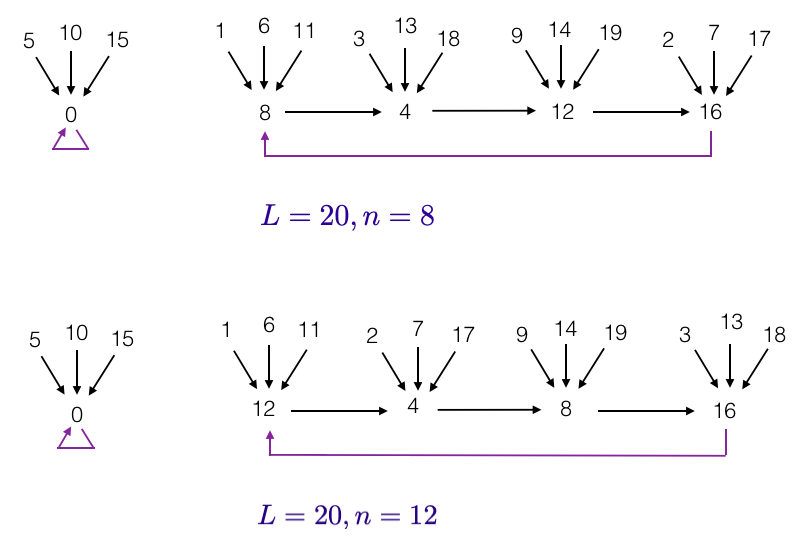
Figure 4. The two Zoloterev graphs $Z(8,20)$ and $Z(12,20)$ are isomorphic. Each of them has $15$ leaves, no branches, $5$ roots, and $2$ connected components.

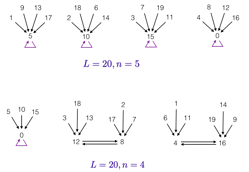
Figure 5. Bottom: $Z(4,20)$ has $15$ leaves, $5$ roots, $0$ branches, and $3$ connected components. Top: $Z(5,20)$ has $16$ leaves, $4$ roots, $0$ branches, and $4$ connected components.

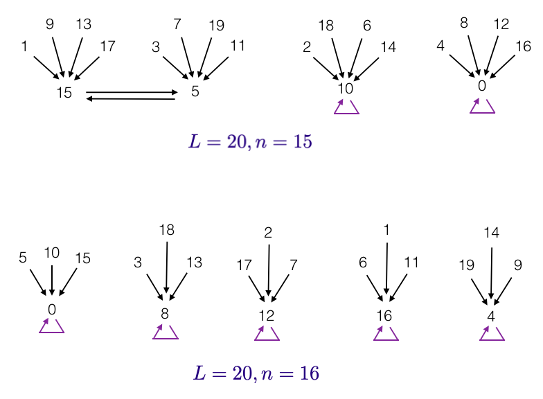
Figure 6. Here $Z(15,20)$ has $3$ connected components, and $4$ roots. $Z(16,20)$ has $5$ connected components, and $5$ roots.

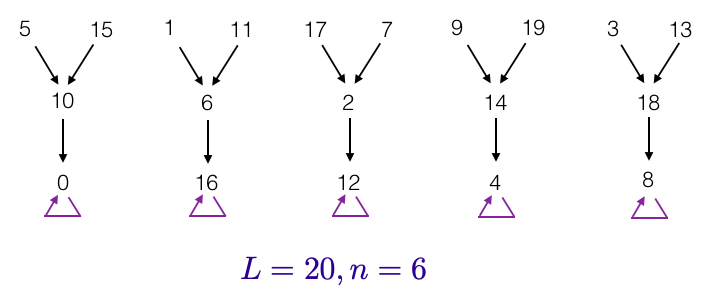
Figure 7. $Z(6,20)$ has $10$ leaves, $5$ branches, $5$ roots, and $5$ connected components.

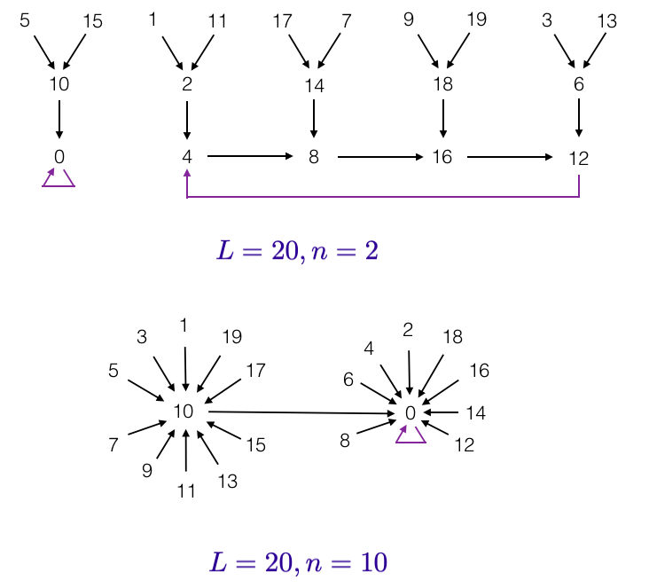
Figure 8. Top: the Zolotarev graph $Z(2,20)$ has $10$ leaves, $5$ roots, and $5$ branch integers. It has $2$ connected components.
Bottom: $Z(10,20)$ has $18$ leaves, $2$ roots, $0$ branches, and just $1$ connected component.

References

- [1] Erich Hecke, Über Modulfunktionen und die Dirichletschen Reihen mit Eulerscher Produktentwicklung. I., Mathematsche Annalen. 1937 doi:10.1007/BF01594160
- [2] C. D. Bennett and E. Mosteig, On the collection of integers that index the fixed points of maps on the space of rational functions, in: Tapas in Experimental Mathematics, Contemporary Mathematics, 457 (American Mathematical Society, Providence, RI, 2008), 53–67.
- [3] George Boros, John Little, Victor Moll, Ed Mosteig, and Richard Stanley, A map on the space of rational functions, Rocky Mountain Journal of Mathematics, Volume 35, Number 6, (2005), 1861–1880.
- [4] Juan B. Gil and Sinai Robins, Hecke operators on rational functions I, Forum Mathematicum, vol. 17, no. 4, 2005, 519–554. https://doi.org/10.1515/form.2005.17.4.519
- [5] Victor H. Moll, Sinai Robins, and Kirk Soodhalter, The action of Hecke operators on hypergeometric series, Journal of the Australian Mathematical Society, Volume 89, Issue 1 , August 2010 , 51–74.
- [6] Elias M. Stein and Rami Shakarchi, Real Analysis, Princeton Lectures in Analysis, (2005).
- [7] Joseph Silverman, The arithmetic of dynamical systems, Springer, Graduate Texts in Mathematics (GTM, volume 241), (2007), 1–515.
- [8] Robert Benedetto, Patrick Ingram, Rafe Jones, Michelle Manes, Joseph H. Silverman, and Thomas J. Tucker, Current trends and open problems in arithmetic dynamics, Bulletin of the AMS, Vol. 56, Number 4, October 2019, 611–685.
- [9] Giancarlo Travaglini, Number theory, Fourier analysis and geometric discrepancy, London Mathematical Society Student Texts, 81. Cambridge University Press, Cambridge (2014), 1–240.
- [10] A. W. Ingleton, Circulant Matrices, J. London Mathematical Society, s1-31: 445-460 https://doi.org/10.1112/jlms/s1-31.4.445
- [11] Wolfram Research, Inc., Wolfram—Alpha Notebook Edition, Champaign, IL (2021).
- [12] Richard Stanley, Enumerative Combinatorics, Volume 1, Cambridge Studies in Advanced Mathematics, Cambridge University Press, (1997).
- [13] Rodney Coleman, On the image of Euler’s totient function. 2009. ffhal-00423598f