Probabilistic Programming with Programmable
Variational Inference

Abstract.

Compared to the wide array of advanced Monte Carlo methods supported by modern probabilistic programming languages (PPLs), PPL support for variational inference (VI) is less developed: users are typically limited to a predefined selection of variational objectives and gradient estimators, which are implemented monolithically (and without formal correctness arguments) in PPL backends. In this paper, we propose a more modular approach to supporting variational inference in PPLs, based on compositional program transformation. In our approach, variational objectives are expressed as programs, that may employ first-class constructs for computing densities of and expected values under user-defined models and variational families. We then transform these programs systematically into unbiased gradient estimators for optimizing the objectives they define. Our design enables modular reasoning about many interacting concerns, including automatic differentiation, density accumulation, tracing, and the application of unbiased gradient estimation strategies. Additionally, relative to existing support for VI in PPLs, our design increases expressiveness along three axes: (1) it supports an open-ended set of user-defined variational objectives, rather than a fixed menu of options; (2) it supports a combinatorial space of gradient estimation strategies, many not automated by today’s PPLs; and (3) it supports a broader class of models and variational families, because it supports constructs for approximate marginalization and normalization (previously introduced only for Monte Carlo inference). We implement our approach in an extension to the Gen probabilistic programming system (genjax.vi, implemented in JAX), and evaluate our automation on several deep generative modeling tasks, showing minimal performance overhead vs. hand-coded implementations and performance competitive with well-established open-source PPLs.

1. Introduction

Variational inference (VI) is a popular approach to two fundamental probabilistic modeling tasks:

• Fitting probabilistic models to data. Given a family of joint probability distributions $\mathcal{P}=\{P_{\theta}(x,y)\mid\theta\in\mathbb{R}^{n}\}$ defined over latent variables $x$ and observed variables $y$, find the one that best explains an observed dataset $\mathbf{y}$. For example, writing $p_{\theta}$ for the probability density function of $P_{\theta}$, we may be interested in finding $\theta\in\mathbb{R}^{n}$ that maximizes the marginal likelihood

  (1) $$p_{\theta}(\mathbf{y})=\int_{X}p_{\theta}(x,\mathbf{y})dx.$$

• Approximating intractable posterior distributions. For a particular probabilistic model $P_{\theta}(x,y)$, find the best approximation to the (usually intractable) posterior distribution $P_{\theta}(x\mid\mathbf{y})$, from a class $\mathcal{Q}=\{Q_{\phi}(x)\mid\phi\in\mathbb{R}^{m}\}$ of tractable approximations (the variational family). For example, again using lower-case letters for probability density functions, we may be interested in finding $\phi$ that minimizes the reverse KL divergence

  (2) $$D_{KL}(Q_{\phi}(x)\,||\,P_{\theta}(x\mid\mathbf{y}))=-\mathbb{E}_{x\sim Q_{\phi}}\!\left[\log\frac{p_{\theta}(x\mid\mathbf{y})}{q_{\phi}(x)}\right].$$

Practitioners often aim to solve both these tasks at once, simultaneously fitting a probabilistic model and approximating its posterior distribution. To do so, one defines a variational objective $\mathcal{F}:\mathcal{P}\times\mathcal{Q}\to\mathbb{R}$, mapping particular distributions $P_{\theta}$ and $Q_{\phi}$ to a scalar loss (or reward). For example, one common choice is the evidence lower bound, or ELBO:

(3) $$\mathbf{ELBO}(P,Q):=\mathbb{E}_{x\sim Q}[\log p(x,\mathbf{y})-\log q(x)]=\log p(\mathbf{y})-D_{KL}(Q(x)||P(x\mid\mathbf{y}))$$

As the decomposition on the right-hand side suggests, maximizing the ELBO simultaneously maximizes the (log) marginal likelihood of the data $\mathbf{y}$ and minimizes the KL divergence of the posterior approximation $Q$ to the posterior. Besides the ELBO, researchers have also proposed many alternative objectives (Dempster et al., 1977; Hinton et al., 1995; Agakov and Barber, 2004; Bornschein and Bengio, 2015; Burda et al., 2016; Ranganath et al., 2016; Rainforth et al., 2018; Sobolev and Vetrov, 2019; Malkin et al., 2022), which formalize the two goals of fitting models and approximating posteriors differently (e.g., by using divergences other than the KL). Once a variational objective has been defined, practitioners aim to find parameters $(\theta,\phi)$ that maximize (or minimize) $\mathcal{F}(P_{\theta},Q_{\phi})$. There are many possible approaches to performing this optimization. The most popular methods rely on gradients $\nabla_{(\theta,\phi)}\mathcal{F}(P_{\theta},Q_{\phi})$ of the objective—or more often, unbiased stochastic estimates of these gradients. Designing and implementing algorithms for estimating these gradients, with sufficiently low variance and computational expense, is the key roadblock on the path from defining a variational inference problem to solving it.

Indeed, although variational inference algorithms have found widespread adoption in Bayesian statistics (Fox and Roberts, 2012; Kucukelbir et al., 2017; Blei et al., 2016; Hoffman et al., 2013; Blei and Jordan, 2006) and in probabilistic deep learning (Kingma and Welling, 2022; Pu et al., 2016; Kingma et al., 2021; Vahdat and Kautz, 2020; Malkin et al., 2022), implementing variational inference algorithms by hand remains a tedious and error-prone endeavor. The key mathematical ingredients specifying a variational inference problem—$\mathcal{P}$, $\mathcal{Q}$, and $\mathcal{F}$—are typically not represented directly in code; rather, the practitioner must:

1. use algebra, probability theory, and calculus to derive a gradient estimator: a way to rewrite the gradient $\nabla_{(\theta,\phi)}\mathcal{F}(P_{\theta},Q_{\phi})$ as an expectation $\mathbb{E}_{y\sim M_{(\theta,\phi)}}[f_{(\theta,\phi)}(y)]$, for some family of distributions $M$ and some family of functions $f$; and then

2. write code to sample $y\sim M_{(\theta,\phi)}$ and evaluate $f_{(\theta,\phi)}(y)$—an unbiased estimate of $\nabla_{(\theta,\phi)}\mathcal{F}(P_{\theta},Q_{\phi})$.

It is often non-trivial to ensure that $M$ and $f$ are faithfully implemented, and that the math used to derive them in the first place is error-free. Small changes to $\mathcal{F}$, $\mathcal{P}$, or $\mathcal{Q}$, or to the gradient estimation strategy employed in step (1), can require large, non-local changes to $M$ and $f$, and in implementing these changes, it is easy to introduce hard-to-detect bugs. When optimization fails, it is often unclear whether the problem is with the math, the code, or just the hyperparameters.

Automation via Probabilistic Programming.

Reflecting the importance of variational inference, many probabilistic programming languages (PPLs) (especially “deep” PPLs, such as Pyro (Bingham et al., 2019), Edward (Tran et al., 2017, 2018), and ProbTorch (Stites et al., 2021)), feature varying degrees of automation for VI workflows. In these languages, users can express both models $\mathcal{P}$ and variational families $\mathcal{Q}$ as probabilistic programs; the system then automates the estimation of gradients for a pre-defined set of supported variational objectives $\mathcal{F}$. This design significantly lowers the cost of implementing and iterating on variational inference algorithms, but several pain points remain:

• Incomplete coverage. Existing PPLs offer limited or no support for many variational objectives, including forward KL objectives (Naesseth et al., 2020); hierarchical, nested, or recursive variational objectives (Ranganath et al., 2016; Zimmermann et al., 2021; Lew et al., 2022); symmetric divergences (Domke, 2021); trajectory-balance objectives (Malkin et al., 2022); SMC-based objectives (Maddison et al., 2017; Gu et al., 2015; Li et al., 2023a; Naesseth et al., 2018); and others. Today’s PPLs also do not automate many powerful gradient estimation strategies, for example those based on measure-valued differentiation (Mohamed et al., 2020).

• Duplicative engineering effort. For PPL maintainers, supporting new gradient estimation strategies or language features requires separately introducing the same logic into the implementations of multiple variational objectives. Because this engineering effort is non-trivial, many capabilities are not uniformly supported. For example, as of this writing, Pyro’s ReweightedWakeSleep objective (Le et al., 2019) does not support minibatching, even though other objectives do. As another example, variance reduction strategies such as data-dependent baselines and enumeration of discrete latents are implemented for the ELBO in Pyro, but not, e.g., for the importance-weighted ELBO.

• Difficulty of reasoning. The monolithic implementations of each variational objective’s gradient estimation logic intertwine various concerns, including log density accumulation, automatic differentiation, gradient propagation through stochastic choices, and variance reduction logic. This can make it difficult to reason about correctness. Indeed, while the community has made tremendous progress in understanding the compositional correctness arguments of an increasingly broad class of Monte Carlo inference methods for probabilistic programs (Ścibior et al., 2017, 2018; Lew et al., 2023a; Lundén et al., 2021; Borgström et al., 2016), pioneering work on correctness for variational inference (Lee et al., 2019, 2023; Li et al., 2023b) has generally focused on specific properties (e.g., smoothness and absolute continuity) in somewhat restricted languages, and not to end-to-end correctness of gradient estimation for variational inference.

This Work.

In this paper, we present a highly modular, programmable approach to supporting variational inference in PPLs. In our approach, all three ingredients of the variational inference problem—$\mathcal{P}$, $\mathcal{Q}$, and $\mathcal{F}$—are encoded as programs in expressive probabilistic languages, which support compositional annotation for specifying the desired mix of gradient estimation strategies. We then use a sequence of modular program transformations—each of which we independently prove correct—to construct unbiased gradient estimators for the user’s variational objective.

Contributions.

This paper contributes:

• Languages for models, variational families, and variational objectives: We present an expressive language for models and variational families (§3.2), similar to Gen, ProbTorch, or Pyro, along with an expressive differentiable language for variational objective functions (§3.3).

• Flexible, modular automation: We automate a broad class of unbiased gradient estimators for variational objectives (§5). New primitive gradient estimation strategies can be added modularly with just a few lines of code, without deeply understanding system internals (Appx. F).

• Formalization: We formalize our approach as a sequence of composable program transformations (§4-5) of simply-typed $\lambda$-calculi for probabilistic programs (§3), and prove the unbiasedness of gradient estimation (under mild technical conditions) by logical relations (§6). Ours is the first formal account of variational inference for PPLs that accounts for the interactions between tracing, density computation, gradient estimation strategies, and automatic differentiation.

• System: We contribute genjax.vi, a performant, GPU-accelerated implementation of our approach in JAX (Frostig et al., 2018), which also extends our formal modeling language with constructs for marginalization and normalization (§7) (Lew et al., 2023a). We also contribute concise, pedagogical Haskell and Julia versions. Our implementations are the first to feature reverse-mode variants of the ADEV algorithm for modularly differentiating higher-order probabilistic programs (Lew et al., 2023b).

• Empirical evaluation: We evaluate genjax.vi on several benchmark tasks, including the challenging Attend-Infer-Repeat model (Eslami et al., 2016). We find that genjax.vi makes it possible to encode new gradient estimators that converge faster and to better solutions than Pyro’s estimators. We also show, for the first time, that a version of ADEV can be scalably and performantly implemented, to deliver competitive performance on realistic probabilistic deep learning workloads.

Programmability is sometimes seen as being at odds with automation. We emphasize that this paper expands the automation provided by the system, relative to existing VI support in PPLs, by automating a combinatorial space of gradient estimators for arbitrary objectives specified as programs (rather than the handful of objectives and estimators supported by existing PPLs).

2. Overview

Fig. 1 illustrates the workflow of a typical user of our system for modular variational inference:

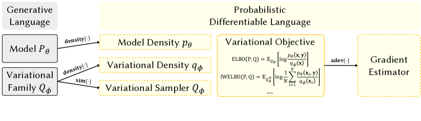
Figure 1. We compose multiple program transformations to automate the construction of unbiased gradient estimators for variational inference. The user begins by writing programs in the generative language (gray) to encode a model and variational family. These programs are compiled into procedures for density evaluation and simulation in the differentiable language (yellow). These automated procedures can be used to concisely define a variational objective. We can then apply the ADEV differentiation algorithm to automatically construct a gradient estimator, which unbiasedly estimates gradients of the variational objective. Solid outlines indicate user-written programs, whereas dashed outlines indicate automatically constructed programs.

An illustration of our pipeline.

• Model and variational programs. The user begins by writing two probabilistic programs in our generative language: a model program and a variational program. The generative language is a trace-based PPL that resembles Pyro (Bingham et al., 2019), ProbTorch (Stites et al., 2021), and Gen (Cusumano-Towner et al., 2019). The model program encodes a family of joint probability distributions $P_{\theta}({x},{y})$, and the variational program encodes a family of distributions $Q_{\phi}({x})$, possible approximations to the posterior $P_{\theta}({x}\mid\mathbf{y})$ for data $\mathbf{y}$.

• Objective function. The user now seeks to find values of $(\theta,\phi)$ that simultaneously (1) fit $P_{\theta}$ to the data $\mathbf{y}$, and (2) make $Q_{\phi}$ close to the posterior $P_{\theta}({x}\mid\mathbf{y})$. To make these informal desiderata precise, the user defines an objective function, using our differentiable language. This language features constructs for taking expectations with respect to, and evaluating densities of, generative language programs, making it easy to concisely express objectives like the ELBO (Eqn. 3).

• Gradient estimator. The final step is to optimize the objective function via stochastic gradient ascent. We construct unbiased gradient estimators for the user’s objective function with an extended version of the ADEV algorithm (Lew et al., 2023b). Users can rapidly explore a combinatorial space of estimation strategies with compositional annotations on their generative programs, to navigate tradeoffs between the variance and the computational cost of the automated gradient estimator.

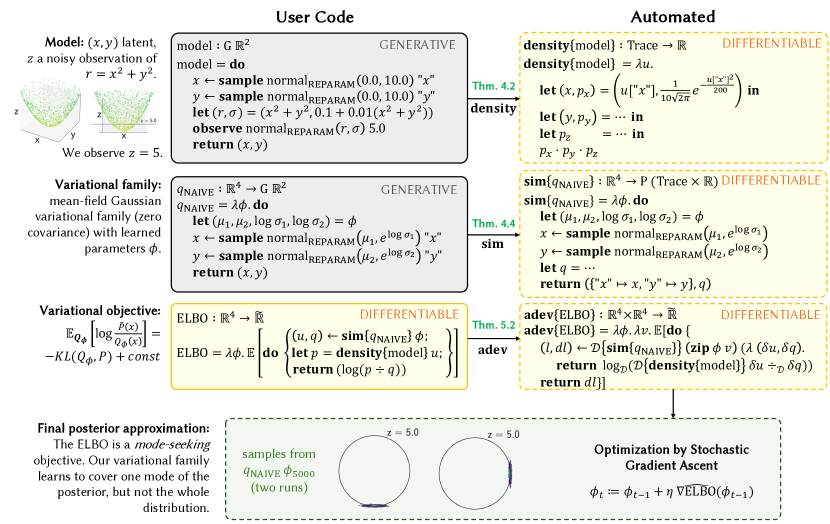
Figure 2. An illustration of our modular approach to automating variational inference, on a toy example. (Top) Users write generative code to define a model and a variational family. Automated program transformations, formalized and proven correct in §4, compile differentiable code for evaluating densities and simulating traces. (Middle) Users write a program in the differentiable language to define a variational objective, in this case the evidence lower bound (ELBO). This code may invoke compiled simulators and density evaluators for generative programs. The adev transformation automates an unbiased gradient estimator for the objective. (Bottom) The gradients are used for optimization, training the variational family to approximate the posterior.

Example.

To make this concrete, consider the toy problem illustrated in Fig.  2, which we seek to solve by training a variational approximation to the posterior. We go through the following steps:

• Define a model. Our model encodes a generative process for points $(x,y,z)$ around a 3D cone. We use sample to sample latents $x$ and $y$ with string-valued names, and observe to condition on the observation that $z=5.0$. Our goal is to infer $(x,y)$ consistent with this observation.

• Define a variational family. In the second panel of Fig. 2, we construct a variational family, a parametric family of possible approximations to the posterior distribution. Our variational inference task will be to learn parameters that maximize the quality of the approximation. Our $\texttt{q}_{\texttt{NAIVE}}$ is a mean-field variational approximation, i.e., it generates $x$ and $y$ independently. Note that primitive distributions (here, normal) are annotated with gradient estimation strategies (here, REPARAM) for propagating derivative information through the corresponding primitive.

• Define a variational objective. We now use the differentiable language to define the objective function we wish to optimize. Three constructs are especially useful: (1) density, which computes or estimates densities of probabilistic programs; (2) sim, which generates a pair $(x,w)$ of a sample and its density from a probabilistic program; and (3) $\mathbb{E}$, which takes the expected value of a stochastic procedure. We use them together to implement the ELBO objective from Eqn. 3.

• Perform stochastic optimization. Our objective is compiled into an unbiased estimator of its gradient with respect to the input parameters $\phi$. We can then apply stochastic optimization algorithms, such as stochastic gradient ascent and ADAM. The bottom of Fig. 2 illustrates samples from $\texttt{q}_{\texttt{NAIVE}}$ after training. Because the ELBO minimizes the reverse (or mode-seeking) KL divergence, our variational approximation learns to hug one edge of the circle-shaped posterior.

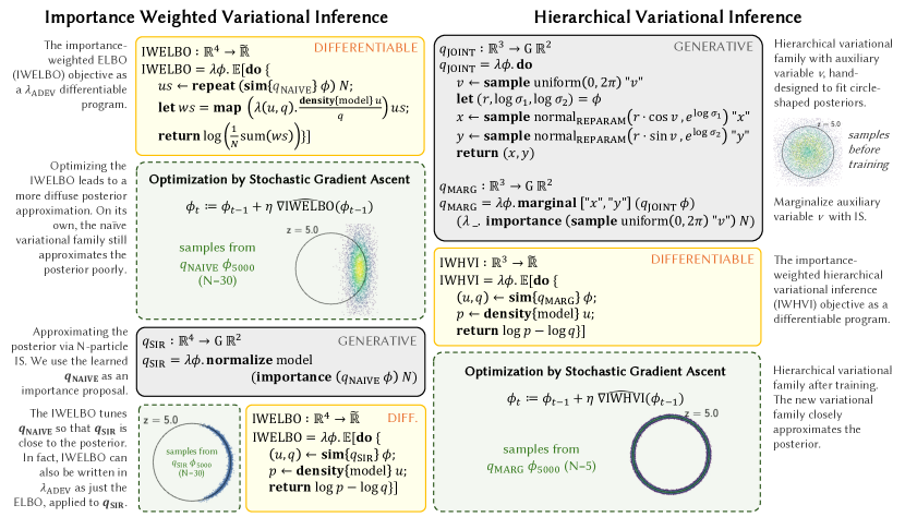
Figure 3. With programmable VI, users can define their own variational objectives, and use new modeling language features to program more expressive models and variational families. Here, we apply importance-weighted VI (Burda et al., 2016) and hierarchical VI (Ranganath et al., 2016; Sobolev and Vetrov, 2019) to the toy problem from Fig. 2.

Better Inference with Programmable Objectives.

To better fit the whole posterior, we will need either a new objective function or a more expressive variational family. Our system’s programmability allows users to quickly iterate within a broad space of VI algorithms. In Fig. 3, we illustrate two possible strategies for improving the posterior approximation:

• Importance-weighted variational inference. On the left side of Fig. 3, we define the IWELBO variational objective (Burda et al., 2016), as the expected value of the process that generates $N$ particles from the variational family $\texttt{q}_{\texttt{NAIVE}}$, and computes a log mean importance weight. This objective does not directly encourage $\texttt{q}_{\texttt{NAIVE}}$ to approximate the posterior well; rather, it encourages $\texttt{q}_{\texttt{NAIVE}}$ to be a good proposal distribution for $N$-particle importance sampling, targeting the posterior. To illustrate this, we define a new probabilistic program $\texttt{q}_{\texttt{SIR}}$, which uses normalize to construct a sampling importance resampling (SIR) approximation to the posterior: it generates $N$ samples from $\texttt{q}_{\texttt{NAIVE}}$, computes importance weights for each sample, and randomly selects a sample to return according to the weights. Drawing samples from $\texttt{q}_{\texttt{SIR}}$, with $N=30$ and $\phi$ set to the parameters that optimized the IWELBO objective, yields a close approximation to a larger portion of the posterior. (In fact, the IWELBO objective can be equivalently expressed in our framework as the ordinary ELBO, but applied directly to $\texttt{q}_{\texttt{SIR}}$ rather than to $\texttt{q}_{\texttt{NAIVE}}$.)

• Hierarchical variational families. On the right side of Fig. 3, we define a better variational family: $\texttt{q}_{\texttt{MARG}}$. First, we define a hand-designed posterior approximation $\texttt{q}_{\texttt{JOINT}}$, which extends $\texttt{q}_{\texttt{NAIVE}}$ with an auxiliary variable $v$, to allow it to better fit circle-shaped posteriors. We cannot directly use $\texttt{q}_{\texttt{JOINT}}$ with the ELBO objective, however, because it is defined over the space of triples $(v,x,y)$, not the space of pairs $(x,y)$ as in our model. The marginal construct shrinks the sample space back down to just $(x,y)$, approximating the marginal density $\texttt{q}_{\texttt{MARG}}(x,y)$ using importance sampling. The resulting algorithm is an instance of importance weighted HVI (IWHVI) (Sobolev and Vetrov, 2019).

3. Syntax and Semantics

Shared Core

$$\text{Ground types }\sigma\,::=\, 1\mid\mathbb{B}\mid\mathbb{I}\mid\mathbb{R}_{>0}\mid\mathbb{R}_{\geq 0}\mid\mathbb{R}\mid\mathbb{R}^{*}\mid\text{Str}\mid\sigma_{1}\times\sigma_{2}\quad\quad\quad\quad\text{Types }\tau\,::=\,\sigma\mid D~{}\sigma\mid\tau_{1}\to\tau_{2}\mid\tau_{1}\times\tau_{2}$$

$$\text{Terms }t\,::=\, ()\mid r\mid c\mid x\mid\lambda x.t\mid t_{1}\,t_{2}\mid(t_{1},t_{2})\mid\pi_{1}~{}t\mid\pi_{2}~{}t\mid\mathbf{T}\mid\mathbf{F}\mid\textbf{if }t\textbf{ then }t_{1}\textbf{ else }t_{2}$$

$$\text{Primitives }c\,::=\, +\mid+^{*}\mid<~{}\mid\textbf{normal}_{\text{REPARAM}}\mid\textbf{normal}_{\text{REINFORCE}}\mid\textbf{flip}_{\text{REINFORCE}}\mid\textbf{flip}_{\text{ENUM}}\mid\textbf{flip}_{\text{MVD}}\mid\dots$$

$t:\mathbb{R}^{*}$ $t:\mathbb{R}$ $+:\mathbb{R}\times\mathbb{R}\to\mathbb{R}$ $+^{*}:\mathbb{R}^{*}\times\mathbb{R}^{*}\to\mathbb{R}^{*}$ $<~{}:\mathbb{R}^{*}\times\mathbb{R}^{*}\to\mathbb{B}$ $\textbf{normal}_{\text{REPARAM}}:\mathbb{R}\times\mathbb{R}_{>0}\to D\,\mathbb{R}$ $\textbf{normal}_{\text{REINFORCE}}:\mathbb{R}\times\mathbb{R}_{>0}\to D\,\mathbb{R}^{*}$ $\textbf{flip}_{\text{MVD}}:\mathbb{I}\to D\,\mathbb{B}$

$\llbracket 1\rrbracket=\{()\}$  $\llbracket\mathbb{I}\rrbracket=[0,1]$  $\llbracket\mathbb{R}\rrbracket=\llbracket\mathbb{R}^{*}\rrbracket=\mathbb{R}$  $\llbracket D~{}\sigma\rrbracket=\text{Prob}_{\ll\mathcal{B}_{\sigma}}~{}\llbracket\sigma\rrbracket$  $\llbracket\mathbf{normal}_{\text{REPARAM}}\rrbracket=\llbracket\textbf{normal}_{\text{REINFORCE}}\rrbracket=\lambda(\mu,\sigma).\mathcal{N}(\mu,\sigma)$

Generative Probabilistic Programming ($\lambda_{\text{Gen}}$)

$$\text{Types }\tau\,::=\, G\,\tau\text{ (generative programs)}$$

$$\text{Terms }t\,::=\, \textbf{return}\,t\mid\textbf{sample}\,t_{1}\,t_{2}\mid$$

$$\textbf{observe}\,t_{1}\,t_{2}\mid\textbf{do}\{m\}$$

$$m\,::=\, t\mid x\leftarrow t;m$$

$t:\tau$ $\textbf{return}\,t:G\,\tau$ $t_{1}:{D}~{}\sigma$ $t_{2}:\text{Str}$ $\textbf{sample}\,t_{1}\,t_{2}:G\,\sigma$ $t_{1}:{D}~{}\sigma$ $t_{2}:\sigma$ $\textbf{observe}\,t_{1}\,t_{2}:G\,1$ $t:G\,\tau$ $\textbf{do}\{t\}:G\,\tau$
$t:G\,\tau_{1}$  $x:\tau_{1}\vdash\textbf{do}\,\{m\}:G\,\tau_{2}$ $\textbf{do}\{x\leftarrow t;m\}:G\,\tau_{2}$

$\llbracket G~{}\tau\rrbracket=\text{Meas}_{\ll\mathcal{B}_{\mathbb{T}}}^{DS}~{}\mathbb{T}\times(\mathbb{T}\Rightarrow\llbracket\tau\rrbracket)$

$$\llbracket\textbf{return}~{}t\rrbracket_{1}(\gamma,U) =\delta_{\{\}}(U)$$

$$\llbracket\textbf{return}~{}t\rrbracket_{2}(\gamma,u) =\llbracket t\rrbracket(\gamma)$$

$$\llbracket\textbf{sample}~{}t_{1}~{}t_{2}\rrbracket_{1}(\gamma,U) =\int\llbracket t_{1}\rrbracket(\gamma,dv)\delta_{\{\llbracket t_{2}\rrbracket(\gamma)\mapsto v\}}(U)$$

$$\llbracket\textbf{sample}~{}t_{1}~{}t_{2}\rrbracket_{2}(\gamma,u) =u[\llbracket t_{2}\rrbracket(\gamma)]$$

$$\llbracket\textbf{observe}~{}t_{1}~{}t_{2}\rrbracket_{1}(\gamma,U) =\frac{d(\llbracket t_{1}\rrbracket(\gamma))}{d\mathcal{B}_{\sigma}}(\llbracket t_{2}\rrbracket(\gamma))\delta_{\{\}}(U)$$

$$\llbracket\textbf{observe}~{}t_{1}~{}t_{2}\rrbracket_{2}(\gamma,u) =()$$

$$\llbracket\textbf{do}\{x\leftarrow t;m\}\rrbracket_{1}(\gamma,U) =\int\llbracket t\rrbracket_{1}(\gamma,du_{1})$$

$$\quad\int\llbracket\textbf{do}\{m\}\rrbracket_{1}(\gamma^{\prime},du_{2})$$

$$\quad\quad\delta_{u_{1}\mathbin{+\mkern-5.0mu+}u_{2}}(U)\cdot\textit{disj}(u_{1},u_{2})$$

$$\text{where }\gamma^{\prime} =\gamma[x\mapsto\llbracket t\rrbracket_{2}(\gamma,u_{1})]$$

$$\llbracket\textbf{do}\{x\leftarrow t;m\}\rrbracket_{2}(\gamma,u) =\llbracket\textbf{do}\{m\}\rrbracket_{2}(\gamma^{\prime},u^{\prime})$$

$$\text{where }\gamma^{\prime} =\gamma[x\mapsto\llbracket t\rrbracket_{2}(\gamma,u)]$$

$$\text{and }u^{\prime} =\pi_{2}(\textit{split}_{\llbracket t\rrbracket_{1}(\gamma)}(u))$$

Differentiable Probabilistic Programming ($\lambda_{\text{ADEV}}$)

$$\text{Types }\tau\,::=\, P~{}\tau\mid\widetilde{\mathbb{R}}\mid\text{Trace}$$

$$\text{Terms }t\,::=\, \mathbb{E}~{}t\mid\textbf{return}~{}t\mid\textbf{sample}~{}t\mid\textbf{do}\{m\}\mid$$

$$\mathbf{score}~{}t\mid\{\}\mid\{t_{1}\mapsto t_{2}\}\mid t_{1}\mathbin{+\mkern-5.0mu+}t_{2}\mid t_{1}[t_{2}]$$

$$m\,::=\, t\mid x\leftarrow t;m$$

$t:\tau$ $\textbf{return}\,t:P\,\tau$ $t:{D}~{}\sigma$ $\textbf{sample}\,t:P\,\sigma$
$t:\mathbb{R}_{\geq 0}$ $\mathbf{score}~{}t:P\,1$ $t:P\,\tau$ $\textbf{do}\{t\}:P\,\tau$ $t:P\,\mathbb{R}$ $\mathbb{E}~{}t:\widetilde{\mathbb{R}}$ $t:P\,\tau_{1}$  $x:\tau_{1}\vdash\textbf{do}\,\{m\}:P\,\tau_{2}$ $\textbf{do}\{x\leftarrow t;m\}:P\,\tau_{2}$

$\llbracket P~{}\tau\rrbracket=\text{Meas}~{}\llbracket\tau\rrbracket\;\mid\;\llbracket\widetilde{\mathbb{R}}\rrbracket=\text{Meas}~{}\mathbb{R}\;\mid\;\llbracket\text{Trace}\rrbracket=\mathbb{T}$

$$\llbracket\textbf{return}~{}t\rrbracket(\gamma,U) =\delta_{\llbracket t\rrbracket(\gamma)}(U)$$

$$\llbracket\textbf{sample}~{}t\rrbracket(\gamma,U) =\llbracket t\rrbracket(\gamma,U)$$

$$\llbracket\textbf{score}~{}t\rrbracket(\gamma,U) =\llbracket t\rrbracket(\gamma)\cdot\delta_{()}(U)$$

$$\llbracket\textbf{do}\{x\leftarrow t;m\}\rrbracket(\gamma,U) =\int\llbracket t\rrbracket(\gamma,du_{1})$$

$$\quad\quad\;\llbracket\textbf{do}\{m\}\rrbracket(\gamma[x\mapsto u_{1}],U)$$

$$\llbracket\mathbb{E}~{}t\rrbracket(\gamma,U) =\llbracket t\rrbracket(\gamma,U)$$

$$\llbracket\{\}\rrbracket(\gamma) =\{\}$$

$$\llbracket\{t_{1}\mapsto t_{2}\}\rrbracket(\gamma) =\{\llbracket t_{1}\rrbracket(\gamma)\mapsto\llbracket t_{2}\rrbracket(\gamma)\}$$

$$\llbracket t_{1}\mathbin{+\mkern-5.0mu+}t_{2}\rrbracket(\gamma) =\begin{cases}u_{1}\mathbin{+\mkern-5.0mu+}u_{2}&\text{ if }\textit{disj}(u_{1},u_{2})\\ \{\}&\text{ otherwise}\end{cases}$$

$$\text{where }u_{i} =\llbracket t_{i}\rrbracket(\gamma)$$

$$\llbracket t_{1}[t_{2}]\rrbracket(\gamma) =\begin{cases}u[v]&\text{ if }v\in u\\ \text{default}_{\sigma}&\text{ otherwise}\end{cases}$$

$$\text{where }(u,v) =(\llbracket t_{1}\rrbracket(\gamma),\llbracket t_{2}\rrbracket(\gamma))$$

Grammar and typing rules for our languages.

Figure 4. Grammars, selected typing rules, and selected denotations for our core languages $\lambda_{\text{Gen}}$ and $\lambda_{ADEV}$.

We now formalize the core of our approach. Although our formal model lacks several features of our full language (see §7 and Appx. A), it is still expressive, featuring higher-order functions, continuous and discrete sampling, stochastic control flow, and discontinuous branches. Ultimately, our formalization aims to give an account of how user programs representing models, variational families, and variational objectives are transformed into compiled programs representing unbiased gradient estimators. We begin in this section by introducing two calculi for generative and differentiable probabilistic programming (Fig. 4).

3.1. Shared Core

3.1.1. Syntax

The top of Fig. 4 presents the shared core, the $\lambda$-calculus on which both our languages build. It is largely standard, with functions, tuples, if statements, and ground types for Booleans, strings, and numbers, but two aspects merit further discussion:

• Smooth and non-smooth reals. First, following Lew et al. (2023b), we have two types for real numbers, $\mathbb{R}$ and $\mathbb{R}^{*}$. Intuitively, the type $\mathbb{R}$ is the type of “real numbers that must be used differentiably,” whereas the type $\mathbb{R}^{*}$ is the type of “real numbers that may be manipulated in any (measurable) way.” These constraints are enforced by the types of primitive functions: non-smooth primitives like $<~{}:\mathbb{R}^{*}\times\mathbb{R}^{*}\to\mathbb{B}$ only accept $\mathbb{R}^{*}$ inputs. Smooth primitives, by contrast, come in two varieties, smooth versions (e.g. $+:\mathbb{R}\times\mathbb{R}\to\mathbb{R}$) and non-smooth versions (e.g. $+^{*}:\mathbb{R}^{*}\times\mathbb{R}^{*}\to\mathbb{R}^{*}$). We allow implicit promotion of terms of type $\mathbb{R}^{*}$ into terms of type $\mathbb{R}$.

• Primitive distributions. The shared core includes a type $D~{}\sigma$ of primitive probability distributions over ground types $\sigma$. Again following Lew et al. (2023b), we expose multiple versions of each primitive, e.g. $\textbf{normal}_{\text{REPARAM}}$ and $\textbf{normal}_{\text{REINFORCE}}$. All versions denote the same distribution, and so our correctness results (which are phrased in terms of our denotational semantics) ensure that gradients will target the same objective no matter which version a program uses (Thm. 5.2). But different versions of the same primitive employ different estimation strategies for propagating derivatives, striking different trade-offs between variance and cost. Furthermore, because different estimation strategies may place different requirements on the user’s program, the typing rules for different versions of the same primitive may differ. For example, $\textbf{normal}_{\text{REINFORCE}}$ constructs a distribution of type $D~{}\mathbb{R}^{*}$, meaning that probabilistic programs that draw samples from it can freely manipulate those samples. By contrast, $\textbf{normal}_{\text{REPARAM}}$ constructs a distribution of type $D~{}\mathbb{R}$, so samples from $\textbf{normal}_{\text{REPARAM}}$ must be used smoothly.

3.1.2. Denotational Semantics.

We assign to each type $\tau$ a mathematical space $\llbracket\tau\rrbracket$, and interpret an open term $\Gamma\vdash t:\tau$ as a map from $\llbracket\Gamma\rrbracket\coloneqq\prod_{x\in\Gamma}\llbracket\Gamma(x)\rrbracket$, the space of environments for context $\Gamma$, to $\llbracket\tau\rrbracket$, the space of results to which $t$ can evaluate. Formally, we work in the category of quasi-Borel spaces (Heunen et al., 2017), but to ease exposition, we present our semantics in terms of standard measure theory when possible. So, for example, we write that $\llbracket\mathbb{R}\rrbracket$ is the measurable space $(\mathbb{R},\mathcal{B}(\mathbb{R}))$, that $\llbracket\sigma_{1}\times\sigma_{2}\rrbracket$ is the product of the measurable spaces $\llbracket\sigma_{1}\rrbracket$ and $\llbracket\sigma_{2}\rrbracket$, and so on, but with the implicit understanding that these can equivalently be viewed as quasi-Borel spaces. For semantics of higher-order types, we use quasi-Borel spaces explicitly (e.g., we set $\llbracket\tau_{1}\to\tau_{2}\rrbracket$ to $\llbracket\tau_{1}\rrbracket\Rightarrow\llbracket\tau_{2}\rrbracket$, the quasi-Borel space of quasi-Borel maps from $\llbracket\tau_{1}\rrbracket$ to $\llbracket\tau_{2}\rrbracket$).

To give a semantics to our primitive distributions, we need to first assign to each ground type $\sigma$ a base measure $\mathcal{B}_{\sigma}$ over $\llbracket\sigma\rrbracket$: for discrete types $\sigma\in\{1,\mathbb{B},\text{Str}\}$, we set $\mathcal{B}_{\sigma}(U)=|U|$, the counting measure, and for continuous types $\sigma\in\{\mathbb{R},\mathbb{R}^{*}\}$, we set $\mathcal{B}_{\sigma}(U)=\int_{\mathbb{R}}1_{U}(u)du$, the Lebesgue measure. Given two ground types $\sigma_{1}$ and $\sigma_{2}$, the base measure of the product, $\mathcal{B}_{\sigma_{1}\times\sigma_{2}}$, is $\mathcal{B}_{\sigma_{1}}\otimes\mathcal{B}_{\sigma_{2}}$, the product of the base measures for each type. With base measures in hand, we can define $\llbracket D~{}\sigma\rrbracket\coloneqq\text{Prob}_{\ll\mathcal{B}_{\sigma}}\llbracket\sigma\rrbracket$, the space of probability measures on $\llbracket\sigma\rrbracket$ that are absolutely continuous with respect to $\mathcal{B}_{\sigma}$. Absolute continuity ensures that these distributions have density functions.

3.2. Generative Probabilistic Programming with $\lambda_{\text{Gen}}$

Users write probabilistic models and variational families in $\lambda_{\text{Gen}}$, which extends the shared core with a monadic type $G~{}\tau$ of generative programs (Fig. 4, left). Examples of programs in $\lambda_{\text{Gen}}$ include the model and variational programs (model and $\texttt{q}_{\texttt{NAIVE}}$) in Fig. 2.

3.2.1. Syntax

Syntactically, programs of type $G~{}\tau$ interleave standard functional programming logic (from the shared core) with two new kinds of statements: sample and observe. The sample statement takes as input a probability distribution to sample (of type $D~{}\sigma$) and a unique name for the random variable being sampled (of type Str). The observe statement takes as input a probability distribution representing a likelihood (of type $D~{}\sigma$), and a value representing an observation (of type $\sigma$). A generative program can include many calls to sample and observe, ultimately inducing an unnormalized joint distribution over traces: finite dictionaries mapping the names of random variables to sampled values. Intuitively, ignoring the observe statements in a program, we can read off a sampling distribution over traces—the prior. The observe statements then reweight each possible execution’s trace by the likelihoods accumulated during that execution, yielding an unnormalized posterior over traces.

3.2.2. Denotational Semantics

Formally, we write $\mathbb{T}$ for the space of possible traces. It arises as a countable disjoint union, indexed by possible trace shapes (finite partial maps from string-valued names $k$ to corresponding ground types $\sigma_{k}$), of product spaces $\prod_{k}\llbracket\sigma_{k}\rrbracket$. We can also define a base measure $\mathcal{B}_{\mathbb{T}}$ over $\mathbb{T}$, by summing product measures for each possible trace shape:

$$\mathcal{B}_{\mathbb{T}}(U)\coloneqq\sum_{s\subseteq\text{Str}\times\Sigma}\left(\bigotimes_{(k,\sigma_{k})\in s}\mathcal{B}_{\sigma_{k}}\right)(\{\textit{values}(u)\mid u\in U\wedge\textit{shape}(u)=s\}).$$

Generative programs (of type $G~{}\tau$) induce measures $\mu$ on $\mathbb{T}$ that satisfy two properties: they are absolutely continuous with respect to $\mathcal{B}_{\mathbb{T}}$ (and therefore have a well-defined notion of trace density $\frac{d\mu}{d\mathcal{B}_{\mathbb{T}}}$), and they are discrete-structured: for $(\mu\otimes\mu)$-almost-all pairs of traces $(u_{1},u_{2})$, either $u_{1}=u_{2}$, or there exists a string $s$ present in both $u_{1}$ and $u_{2}$ such that $u_{1}[s]\neq u_{2}[s]$. In words, if two distinct traces are both in the support of a generative program, then in the two executions that those traces represent, there must have been some sample statement at which different choices were made for the same random variable. We write $\text{Meas}_{\ll\mathcal{B}_{\mathbb{T}}}^{DS}~{}\mathbb{T}$ for the space of measures on $\mathbb{T}$ satisfying these two properties. The semantics then assigns $\llbracket G~{}\tau\rrbracket\coloneqq\text{Meas}_{\ll\mathcal{B}_{\mathbb{T}}}^{DS}~{}\mathbb{T}\times(\mathbb{T}\Rightarrow\llbracket\tau\rrbracket)$: a generative program denotes both a (well-behaved) measure on traces, and a return-value function that given a trace, computes the program’s $\llbracket\tau\rrbracket$-valued result when its random choices are as in the trace.

The semantics for terms of type $G~{}\tau$ (Fig. 4, bottom left) give a formal account of how a generative program’s source code yields a particular measure on traces and return-value function. We write $\llbracket\cdot\rrbracket_{i}$ for $\pi_{i}\circ\llbracket\cdot\rrbracket$, so that $\llbracket\cdot\rrbracket_{1}$ computes the measure on traces and $\llbracket\cdot\rrbracket_{2}$ computes the return-value function. In Appx. E, we show that our term semantics really does map every program of type $G~{}\tau$ a well-behaved measure over traces, i.e., the absolute continuity and discrete-structure requirements are satisfied by our definitions. The semantics of each probabilistic programming construct can be understood in terms of its trace distribution and return value function:

• $\textbf{return}~{}t$: The simplest generative programs deterministically compute a return value $t$. These programs denote deterministic (Dirac delta) distributions on the empty trace $\{\}$, because they make no random choices. The return value function $\llbracket\textbf{return}~{}t\rrbracket_{2}(\gamma)$ then maps any trace $u$ to the program’s return value, $\llbracket t\rrbracket(\gamma)$.

• $\textbf{sample}~{}t_{1}~{}t_{2}$: Slightly more complicated, the $\textbf{sample}~{}t_{1}~{}t_{2}$ command denotes a measure over singleton traces $\{\textit{name}\mapsto\textit{value}\}$, namely the pushforward of the measure $\llbracket t_{1}\rrbracket(\gamma)$ by the function $\lambda v.\{\llbracket t_{2}\rrbracket(\gamma)\mapsto v\}$. The return value function for $\textbf{sample}~{}t_{1}~{}t_{2}$ statements accepts a trace $u$ and looks up the value associated with the name $\llbracket t_{2}\rrbracket(\gamma)$, if it exists. We define $u[\textit{name}]$ to return the value associated with name in $u$, if name is a key in $u$, and otherwise to return a default value of the appropriate type.

• $\textbf{observe}~{}t_{1}~{}t_{2}$: Like return, the statement $\textbf{observe}~{}t_{1}~{}t_{2}$ makes no random choices, and thus has an empty trace. But it denotes a scaled Dirac delta measure: the measure it assigns to the empty trace is equal to the density of the value $\llbracket t_{2}\rrbracket(\gamma)$ under the measure $\llbracket t_{1}\rrbracket(\gamma)$.

• $\textbf{do}\{x\leftarrow t;m\}$: Sequencing two generative programs concatenates their traces (which we write using the $\mathbin{+\mkern-5.0mu+}$ concatenation operator). The helper $\textit{disj}:\mathbb{T}\times\mathbb{T}\to\{0,1\}$ checks whether the names used by each of two traces are distinct, returning $1$ if so and $0$ otherwise. We use it in our definition of $\llbracket\textbf{do}\{x\leftarrow t;m\}\rrbracket$ to model that when a program uses the same name twice in a single execution, a runtime error is raised: the semantics assigns measure 0 to those executions, leaving measure $<1$ for the remaining, valid executions.

3.3. Differentiable Probabilistic Programming with $\lambda_{\text{ADEV}}$

3.3.1. Syntax

The right panel of Fig. 4 presents a separate extension of the shared core, $\lambda_{\text{ADEV}}$, a lower-level language for differentiable probabilistic programming (Lew et al., 2023b). Like $\lambda_{\text{Gen}}$, $\lambda_{\text{ADEV}}$ adds a monadic type for probabilistic computations, $P~{}\tau$, which supports the sampling of primitive distributions (with sample), deterministic computation (with return), scoring by multiplicative density factors (score), and sequencing (with do). But $\lambda_{\text{ADEV}}$ probabilistic programs do not denote distributions on traces, and the sample statements do not specify names for random variables. Rather, programs directly denote (quasi-Borel) measures on output types $\tau$.

Even so, we do include syntax for constructing and manipulating traces as data. This is because, in $\S\ref{sec:gen-transformations}$, we will develop program transformations that turn $\lambda_{\text{Gen}}$ programs into $\lambda_{\text{ADEV}}$ programs that (differentiably) simulate and evaluate densities of reified trace data structures.

The language also features an expected value operator $\mathbb{E}$, of type $P~{}\mathbb{R}\to\widetilde{\mathbb{R}}$. Terms of type $\widetilde{\mathbb{R}}$ intuitively represent “losses (i.e., objectives) that can be unbiasedly estimated.” The ultimate goal of a user in $\lambda_{\text{ADEV}}$ is to write an objective function of type $\mathbb{R}^{n}\to\widetilde{\mathbb{R}}$ (where $\mathbb{R}^{n}=\mathbb{R}\times\cdots\times\mathbb{R}$), and then use automatic differentiation of expected values (§5) to obtain a gradient estimator for the loss function it denotes. These loss functions can be constructed by taking expectations of probabilistic programs (using $\mathbb{E}$) or by composing existing losses using new primitives (e.g., $+_{\widetilde{\mathbb{R}}}$, $\times_{\widetilde{\mathbb{R}}}$, and $\text{exp}_{\widetilde{\mathbb{R}}}$). Example $\lambda_{\text{ADEV}}$ programs include the objectives defined in §2 (ELBO, IWELBO, and IWHVI), as well as the automatically compiled programs on the right-hand side of Fig. 2.

3.3.2. Denotational Semantics

Semantically, $P~{}\tau$ is the space of quasi-Borel measures on $\llbracket\tau\rrbracket$. The type $\widetilde{\mathbb{R}}$ has the same denotation as $P~{}\mathbb{R}$, but cannot be used monadically (i.e., it composes in a more restricted way than $P~{}\mathbb{R}$). This is because it is intended to represent an unbiased estimator of a particular real number. For example, suppose $p:P~{}\mathbb{R}$ denotes a probability measure over the reals with expected value $0$. Then $\mathbb{E}~{}p:\widetilde{\mathbb{R}}$ denotes the same probability measure, with expected value $0$. But $p$ can be used within larger probabilistic programs; for example, we can write $p_{*}=\textbf{do}\{x\leftarrow p;\textbf{return}\exp(p)\}$, which draws a sample from $p$ and exponentiates it. By Jensen’s inequality, the expected value of $\llbracket p_{*}\rrbracket$ will generally be greater than $e^{0}=1$. By contrast, the term $\mathbb{E}~{}p$ cannot be freely sampled within probabilistic programs, but can be composed with certain special arithmetic operators, so we can write (for example) $p^{*}=\exp_{\widetilde{\mathbb{R}}}(\mathbb{E}~{}p)$. The primitive $\exp_{\widetilde{\mathbb{R}}}$ uses special logic to construct an unbiased estimator of $e^{x}$ given an unbiased estimator of $x$, so the program $p^{*}$ denotes a probability distribution that does have expectation $e^{0}=1$.

4. Compiling Differentiable Simulators and Density Evaluators

Spec	Syntax  $\vdash t:\sigma\to G~{}\tau\implies\vdash\mathbf{density}\{t\}:\sigma\to\text{Trace}\to\mathbb{R}$ Semantics  $\llbracket\mathbf{density}\{t\}\rrbracket(\theta)=\frac{d\llbracket t\rrbracket_{1}(\theta)}{d\mathcal{B}_{\mathbb{T}}}$
Wrapper	$\mathbf{density}\{t\}\coloneqq\lambda\theta.\lambda u.\textbf{let}~{}(x,w,u^{\prime})=\xi\{t\}(\theta)(u)~{}\textbf{in}~{}\mathbf{if}~{}\textit{isempty}(u^{\prime})~{}\mathbf{then}~{}w~{}\mathbf{else}~{}0$
Helper $\xi$	Syntax  $\Gamma\vdash t:\tau\implies\xi\{\Gamma\}\vdash\xi\{t\}:\xi\{\tau\}$ Semantics  $\forall(\gamma,\gamma^{\prime})\in R^{\xi}_{\Gamma},(\llbracket t\rrbracket(\gamma),\llbracket\xi\{t\}\rrbracket(\gamma^{\prime}))\in R^{\xi}_{\tau}$
on types	$\xi\{\sigma\}$ $\coloneqq\sigma$ $R^{\xi}_{\sigma}$ $\coloneqq\{(x,x)\mid x\in\llbracket\sigma\rrbracket\}$ $\xi\{D~{}\sigma\}$ $\coloneqq\sigma\to\mathbb{R}$ $R^{\xi}_{D~{}\sigma}$ $\coloneqq\{(\mu,\rho)\mid\rho=\frac{d\mu}{d\mathcal{B}_{\sigma}}\}$ $\xi\{\tau_{1}\times\tau_{2}\}$ $\coloneqq\xi\{\tau_{1}\}\times\xi\{\tau_{2}\}$ $R^{\xi}_{\tau_{1}\times\tau_{2}}$ $\coloneqq\{((x,y),(x^{\prime},y^{\prime}))\mid(x,x^{\prime})\in R^{\xi}_{\tau_{1}}\wedge(y,y^{\prime})\in R^{\xi}_{\tau_{2}}\}$ $\xi\{\tau_{1}\to\tau_{2}\}$ $\coloneqq\xi\{\tau_{1}\}\to\xi\{\tau_{2}\}$ $R^{\xi}_{\tau_{1}\to\tau_{2}}$ $\coloneqq\{(f,g)\mid\forall(x,y)\in R^{\xi}_{\tau_{1}},(f(x),g(y))\in R^{\xi}_{\tau_{2}}\}$ $\xi\{G~{}\tau\}$ $\coloneqq\text{Trace}\to\xi\{\tau\}\times\mathbb{R}\times\text{Trace}$ $R^{\xi}_{G~{}\tau}$ $\coloneqq\{((\mu,f),g)\mid\exists h.\forall u\in\mathbb{T}.(f(u),h(u))\in R^{\xi}_{\tau}\;\wedge$ $\quad\quad\quad g=\lambda u.\textbf{let}~{}(u_{1},u_{2})=\textit{split}_{\mu}(u)~{}\textbf{in}(h(u),\frac{d\mu}{dB_{\mathbb{T}}}(u_{1}),u_{2})\}$
on terms	$\xi\{()\}$ $\coloneqq()$ $\xi\{x\}$ $\coloneqq x$ $\xi\{\lambda x.t\}$ $\coloneqq\lambda x.\xi\{t\}$ $\xi\{t_{1}~{}t_{2}\}$ $\coloneqq\xi\{t_{1}\}~{}\xi\{t_{2}\}$ $\xi\{(t_{1},t_{2})\}$ $\coloneqq(\xi\{t_{1}\},\xi\{t_{2}\})$ $\xi\{\pi_{i}~{}t\}$ $\coloneqq\pi_{i}~{}\xi\{t\}$ $\xi\{b\}(b\in\{\mathbf{T},\mathbf{F}\})$ $\coloneqq b$ $\xi\{\mathbf{if}~{}t~{}\mathbf{then}~{}t_{1}~{}\mathbf{else}~{}t_{2}\}$ $\coloneqq\mathbf{if}~{}\xi\{t\}~{}\mathbf{then}~{}\xi\{t_{1}\}~{}\mathbf{else}~{}\xi\{t_{2}\}$ $\xi\{\textbf{normal}_{\textit{strat}}\}$ $\coloneqq\lambda\mu.\lambda\sigma.\lambda x.\frac{1}{\sigma\sqrt{2\pi}}e^{-\frac{1}{2}\left(\frac{x-\mu}{\sigma}\right)^{2}}$ $\xi\{\textbf{flip}_{\textit{strat}}\}$ $\coloneqq\lambda p.\lambda b.\mathbf{if}~{}b~{}\mathbf{then}~{}p~{}\mathbf{else}~{}1-p$ $\xi\{\textbf{return}~{}t\}$ $\coloneqq\lambda u.(\xi\{t\},1,u)$ $\xi\{\textbf{observe}~{}t_{1}~{}t_{2}\}$ $\coloneqq\lambda u.((),\xi\{t_{1}\}(\xi\{t_{2}\}),u)$ $\xi\{\textbf{sample}~{}t_{1}~{}t_{2}\}$ $\coloneqq\lambda u.\textbf{let}~{}(v,w,u^{\prime})=\textit{pop}~{}u~{}\xi\{t_{2}\}$ $\quad\quad\;\;\,\textbf{in}~{}(v,w\cdot\xi\{t_{1}\}(v),u^{\prime})$ $\xi\{\textbf{do}~{}\{x\leftarrow t;m\}\}$ $\coloneqq\lambda u.\textbf{let}~{}(x,w,u^{\prime})=\xi\{t\}(u)~{}\textbf{in}$ $\quad\quad\;\;\,\textbf{let}~{}(y,v,u^{\prime\prime})=\xi\{\textbf{do}\{m\}\}(u^{\prime})~{}\textbf{in}$ $\quad\quad\;\;\,(y,w\cdot v,u^{\prime\prime})$

  Spec Syntax  $\vdash t:\sigma\to G~{}\tau\implies\vdash\mathbf{sim}\{t\}:\sigma\to P~{}(\text{Trace}\times\mathbb{R})$ Semantics  $\llbracket\mathbf{sim}\{t\}\rrbracket(\theta)=(\text{id}\otimes\frac{d\llbracket t\rrbracket_{1}(\theta)}{d\mathcal{B}_{\mathbb{T}}})_{*}\llbracket t\rrbracket_{1}(\theta)$ Wrapper $\mathbf{sim}\{t\}\coloneqq\lambda\theta.\textbf{do}\{(x,w,u)\leftarrow\chi\{t\}(\theta);\textbf{return}~{}(u,w)\}$ Helper $\chi$ Syntax  $\Gamma\vdash t:\tau\implies\chi\{\Gamma\}\vdash\chi\{t\}:\chi\{\tau\}$ Semantics   $\forall(\gamma,\gamma^{\prime})\in R^{\chi}_{\Gamma},(\llbracket t\rrbracket(\gamma),\llbracket\chi\{t\}\rrbracket(\gamma^{\prime}))\in R^{\chi}_{\tau}$  on types $\chi\{\sigma\}$ $\coloneqq\sigma$ $R^{\chi}_{\sigma}$ $\coloneqq\{(x,x)\mid x\in\llbracket\sigma\rrbracket\}$ $\chi\{D~{}\sigma\}$ $\coloneqq P~{}(\sigma\times\mathbb{R})\times(\sigma\to\mathbb{R})$ $R^{\chi}_{D~{}\sigma}$ $\coloneqq\{(\mu,(\nu,\rho))\mid\nu(U)=\int\mu(du)\delta_{\left(u,\frac{d\mu}{d\mathcal{B}_{\sigma}}(u)\right)}(U)\wedge\rho=\frac{d\mu}{d\mathcal{B}_{\sigma}}\}$ $\chi\{\tau_{1}\times\tau_{2}\}$ $\coloneqq\chi\{\tau_{1}\}\times\chi\{\tau_{2}\}$ $R^{\chi}_{\tau_{1}\times\tau_{2}}$ $\coloneqq\{((x,y),(x^{\prime},y^{\prime}))\mid(x,x^{\prime})\in R^{\chi}_{\tau_{1}}\wedge(y,y^{\prime})\in R^{\chi}_{\tau_{2}}\}$ $\chi\{\tau_{1}\to\tau_{2}\}$ $\coloneqq\chi\{\tau_{1}\}\to\chi\{\tau_{2}\}$ $R^{\chi}_{\tau_{1}\to\tau_{2}}$ $\coloneqq\{(f,g)\mid\forall(x,y)\in R^{\chi}_{\tau_{1}},(f(x),g(y))\in R^{\chi}_{\tau_{2}}\}$ $\chi\{G~{}\tau\}$ $\coloneqq P~{}(\chi\{\tau\}\times\mathbb{R}\times\text{Trace})$ $R^{\chi}_{G~{}\tau}$ $\coloneqq\{((\mu,f),\nu)\mid\exists g.\forall u.(f(u),g(u))\in R_{\tau}^{\xi}\wedge$       $\nu=\lambda U.\int\mu(du)1_{U}(g(u),\frac{d\mu}{d\mathcal{B}_{\mathbb{T}}}(u),u)\}$  on terms $\chi\{()\}$ $\coloneqq()$ $\chi\{x\}$ $\coloneqq x$ $\chi\{\lambda x.t\}$ $\coloneqq\lambda x.\chi\{t\}$ $\chi\{t_{1}~{}t_{2}\}$ $\coloneqq\chi\{t_{1}\}~{}\chi\{t_{2}\}$ $\chi\{(t_{1},t_{2})\}$ $\coloneqq(\chi\{t_{1}\},\chi\{t_{2}\})$ $\chi\{\pi_{i}~{}t\}$ $\coloneqq\pi_{i}~{}\chi\{t\}$ $\chi\{b\}(b\in\{\mathbf{T},\mathbf{F}\})$ $\coloneqq b$ $\chi\{\mathbf{if}~{}t~{}\mathbf{then}~{}t_{1}~{}\mathbf{else}~{}t_{2}\}$ $\coloneqq\mathbf{if}~{}\chi\{t\}~{}\mathbf{then}~{}\chi\{t_{1}\}~{}\mathbf{else}~{}\chi\{t_{2}\}$ $\chi\{\textbf{normal}_{\textit{strat}}\}$ $\coloneqq\lambda(\mu,\sigma).(\textbf{do}\{$ $\quad\quad x\leftarrow\textbf{sample}~{}\textbf{normal}_{\textit{strat}}(\mu,\sigma);$ $\quad\quad\textbf{let}~{}\rho=\frac{1}{\sigma\sqrt{2\pi}}e^{-\frac{1}{2}\left(\frac{x-\mu}{\sigma}\right)^{2}};$ $\quad\quad\textbf{return}(x,\rho)$ $\quad\},\lambda x.\frac{1}{\sigma\sqrt{2\pi}}e^{-\frac{1}{2}\left(\frac{x-\mu}{\sigma}\right)^{2}})$ $\chi\{\textbf{flip}_{\textit{strat}}\}$ $\coloneqq\lambda p.(\textbf{do}\{$ $\quad\quad b\leftarrow\textbf{sample}~{}\textbf{flip}_{\textit{strat}}(p);$ $\quad\quad\textbf{let}~{}\rho=\mathbf{if}~{}b~{}\mathbf{then}~{}p~{}\mathbf{else}~{}1-p;$ $\quad\quad\textbf{return}(b,\rho)$ $\quad\},\lambda b.\mathbf{if}~{}b~{}\mathbf{then}~{}p~{}\mathbf{else}~{}1-p)$ $\chi\{\textbf{return}~{}t\}$ $\coloneqq\textbf{return}(\chi\{t\},1,\{\})$ $\chi\{\textbf{observe}~{}t_{1}~{}t_{2}\}$ $\coloneqq\textbf{do}\{$ $\quad\quad\textbf{let}w=\pi_{2}(\chi\{t_{1}\})(\chi\{t_{2}\});$ $\quad\quad\textbf{score}~{}w;\textbf{return}~{}((),w,\{\})$ $\quad\}$ $\chi\{\textbf{sample}~{}t_{1}~{}t_{2}\}$ $\coloneqq\textbf{do}\{$ $\quad\quad(x,w)\leftarrow\pi_{1}(\chi\{t_{1}\});$ $\quad\quad\textbf{return}(x,w,\{\chi\{t_{2}\}\mapsto x\})$ $\quad\}$ $\chi\{\textbf{do}~{}\{x\leftarrow t;m\}\}$ $\coloneqq\textbf{do}\{$ $\quad\quad(x,w,u_{1})\leftarrow\chi\{t\};$ $\quad\quad(y,v,u_{2})\leftarrow\chi\{\textbf{do}\{m\}\};$ $\quad\quad\mathbf{if}\textit{disj}(u_{1},u_{2})~{}\mathbf{then}$ $\quad\quad\quad\textbf{return}~{}(y,w\cdot v,u_{1}\mathbin{+\mkern-5.0mu+}u_{2})$ $\quad\quad\mathbf{else}~{}\textbf{do}\{\textbf{score}~{}0;\textbf{return}~{}(y,0,\{\}))\}$ $\quad\}$ Definitions of our program transformations for density evaluation and traced simulation.

Figure 5. Traced simulation and density evaluation as program transformations from $\lambda_{\text{Gen}}$ to $\lambda_{\text{ADEV}}$.

We now show how to take $\lambda_{\text{Gen}}$ programs and automatically compile them into $\lambda_{\text{ADEV}}$ programs that simulate traces or compute density functions. We introduce two program transformations, sim and density, which take $\lambda_{\text{Gen}}$ terms to $\lambda_{\text{ADEV}}$ terms that implement the desired functionality. The intuition for these transformations is as follows:

• ($\textbf{sim}\{\cdot\}$) At a high level, to simulate traces, we just run the generative program and record the value of every sample we take into a growing trace data structure.

• ($\textbf{density}\{\cdot\}$) To compute the density of a trace, we execute the program, but fix the value of every primitive sample to equal the recorded value from the given trace, and multiply a running joint density by the density for the primitive. For observe, we multiply the running joint density by the density of the primitive evaluated at the value provided to the observe statement.

For example, simulating from the unnormalized model in Fig. 2 and then evaluating the density of the sampled trace — using sim and density as introduced in Fig. 5 — might produce:

$$\textbf{sim}\{\texttt{model}\}\rightsquigarrow(\{``x":0.75,``y":-2.2\},1.3\times 10^{-4}),\quad\textbf{density}\{\texttt{model}\}(\{``x":0.75,``y":-2.2\})=1.3\times 10^{-4}$$

Note that although they are not usually formalized as program transformations or rigorously proven correct, the techniques we describe here are well-known and widely used in the implementations of PPLs, e.g. in Gen, ProbTorch, and Pyro.

Differentiability Properties of Densities.

In the context of variational inference, density functions must satisfy certain differentiability properties—with respect to the parameters being learned, and possibly with respect to the location at which the density is being queried, depending on the gradient estimators one wishes to apply. Previous work has developed specialized static analyses to determine smoothness properties of different parts of programs, in order to reason about gradient estimation for variational inference (Lee et al., 2023). A benefit of our approach is that it greatly simplifies this reasoning: the overall differentiability requirements for gradient estimation are enforced by the type system of the target-language ($\lambda_{\text{ADEV}}$), as in (Lew et al., 2023b). We translate well-typed source-language programs into well-typed target-language density evaluators and trace simulators, which can be composed into well-typed variational objectives. This implies a non-trivial result: the restrictions that $\lambda_{\text{Gen}}$ enforces on models and variational families are sufficient to ensure the necessary differentiability properties for unbiased estimation of variational objective gradients. Furthermore, these guarantees can be modularly extended to new variational objectives, gradient estimation strategies, and modeling language features. We discuss this further at the end of §5.

4.1. Compiling Differentiable Density Evaluators

The density program transformation density is given in Fig. 5 (top). As input, it processes a $\lambda_{\text{Gen}}$ term $t$ of type $\sigma\to G~{}\tau$: a generative program that has some (ground type) parameter or input. The result of the transformation is a $\lambda_{\text{ADEV}}$ term of type $\sigma\to\text{Trace}\to\mathbb{R}$, which, given a parameter $\theta$ and a trace $u$, computes the density of $\llbracket t\rrbracket_{1}(\theta)$ at $u$.

The transformation is only defined for source programs of type $\sigma\to G~{}\tau$, but it is implemented using a helper transformation $\xi$ that is defined at all source-language types. The intended behavior of $\xi$ applied to a source-language term depends on the type of the term; we encode this type-dependent specification into a family of relations $R_{\tau}^{\xi}$ indexed by types $\tau$ (see Fig. 5). Each $R_{\tau}^{\xi}$ is a subset of $\llbracket\tau\rrbracket\times\llbracket\xi\{\tau\}\rrbracket$; if $(x,y)\in R_{\tau}^{\xi}$, it means that it is permissible for $\xi$ to translate a term denoting $x$ into a term denoting $y$. For example, $R_{D~{}\sigma}^{\xi}$ relates measures on $\llbracket\sigma\rrbracket$ to their density functions with respect to $\mathcal{B}_{\sigma}$, to encode that $\xi$ should transform primitive distribution terms into terms that compute primitive distribution densities. More interesting is the specification for $\xi$ on full probabilistic programs, of type $G~{}\tau$. Because the term under consideration may be only part of a larger program, $\xi$ must compute not just a density, but also a return value (for use later in the program) and a remainder of its input trace, containing choices not consumed while processing the current term. The relation $R^{\xi}_{G~{}\tau}$ encodes this intuition using the function $\textit{split}_{\mu}$, which splits a trace $u$ into two parts: the largest subtrace of $u$ in the support of $\mu$ and the remaining subtrace, or, if no such subtrace exists, all of $u$ and the empty trace (see Appx. E for a formal definition).

To prove that $\mathbf{density}$ works correctly, we first prove that $\xi$ satisfies its intended specifications:

Lemma 4.1.

Let $\Gamma\vdash t:\tau$ be an open term of $\lambda_{\text{Gen}}$. Then $\xi\{\Gamma\}\vdash\xi\{t\}:\xi\{\tau\}$ is a well-typed open term of $\lambda_{\text{ADEV}}$, and $\forall(\gamma,\gamma^{\prime})\in R^{\xi}_{\Gamma},(\llbracket\tau\rrbracket(\gamma),\llbracket\xi\{\tau\}\rrbracket(\gamma^{\prime}))\in R^{\xi}_{\tau}$.

The proof (in Appx. E) is by induction, but because the inductive hypothesis is different at each type $\tau$ (depending on our definition of $R_{\tau}^{\xi}$), it is an example of what is often called a logical relations proof. Once it is proven, we are ready to prove the main correctness theorem for densities:

Theorem 4.2.

Let $\vdash t:\sigma\to G~{}\tau$ be a closed $\lambda_{\text{Gen}}$ term for some ground type $\sigma$. Then $\vdash{\mathbf{density}}\{t\}:\sigma\to\text{Trace}\to\mathbb{R}$ is a well-typed $\lambda_{\text{ADEV}}$ term and for all $\theta\in\llbracket\sigma\rrbracket$, $\llbracket\mathbf{density}\{t\}\rrbracket(\theta)$ is a density function for $\pi_{1}(\llbracket t\rrbracket)(\theta)$ with respect to $\mathcal{B}_{\mathbb{T}}$.

Proof.

Fix $\theta\in\llbracket\sigma\rrbracket$ and let $(\mu,f)=\llbracket t\rrbracket(\theta)$. By Lemma 4.1, we have that $(\llbracket t\rrbracket(\theta),\llbracket\xi\{t\}\rrbracket(\theta))\in R^{\xi}_{G~{}\tau}$. Now consider a trace $u\in\mathbb{T}$. The $\mathbf{density}$ macro invokes $\xi\{t\}~{}\theta$ on $u$ to obtain a triple $(x,w,u^{\prime})$. By the definition of $R^{\xi}_{G~{}\tau}$, we have that $w=\frac{d\mu}{d\mathcal{B}_{\mathbb{T}}}(u_{1})$ and $u^{\prime}=u_{2}$, for $(u_{1},u_{2})=\textit{split}_{\mu}(u)$. Recall that if $u$ is in the support of $\mu$, or if no subtrace of $u$ is in the support of $\mu$, then $\textit{split}_{\mu}$ returns $(u,\{\})$, causing $\mathbf{density}$ to enter its $\mathbf{then}$ branch and return $w=\frac{d\mu}{d\mathcal{B}_{\mathbb{T}}}(u_{1})=\frac{d\mu}{d\mathcal{B}_{\mathbb{T}}}(u)$ as desired. If $u$ is not in the support of $\mu$ but has a subtrace that is, then $\textit{split}_{\mu}$ returns that subtrace, along with a non-empty $u_{2}$. In this case the $\mathbf{else}$ branch of $\mathbf{density}$ correctly returns $0$ (because $u$ is not in the support). ∎

4.2. Compiling Differentiable Trace Simulators

The simulation program transformation sim is given in Fig. 5 (bottom). Like density, it processes as input a $\lambda_{\text{Gen}}$ term $t$ of type $\sigma\to G~{}\tau$, but it generates a term of type $P~{}(\text{Trace}\times\mathbb{R})$, satisfying the specification that the pushforward by $\pi_{1}$ is the original program’s measure over traces, $\llbracket t\rrbracket_{1}(\theta)$, and that with probability 1, the second component is the density of $\llbracket t\rrbracket_{1}$ evaluated at the sampled trace. Like density, sim is implemented using a helper macro $\chi$ defined at all types. Fig. 5 presents the logical relations $R^{\chi}_{\tau}$ specifying the helper’s intended behavior on terms of type $\tau$. These relations are simpler than those for $\xi$; for example, on terms of type $G~{}\tau$, $\chi$ has almost the same specification as sim itself, except that it must also compute a return value.

One feature of $\chi$ that is worth noting is its translations of primitives. If a primitive used within a traced probabilistic program is annotated with a gradient estimation strategy, then the translated program uses the same annotated primitive, and then computes a density. This is only well-typed because the density functions of primitives that return $\mathbb{R}$ values (i.e., not $\mathbb{R}^{*}$ values) are smooth. This is not a requirement of ADEV in general, but we require it in order to automate differentiable traced simulation.

To prove correctness, we again begin by showing the helper is sound:

Lemma 4.3.

Let $\Gamma\vdash t:\tau$ be an open term of $\lambda_{\text{Gen}}$. Then $\chi\{\Gamma\}\vdash\chi\{t\}:\chi\{\tau\}$ is a well-typed open term of $\lambda_{\text{ADEV}}$, and $\forall(\gamma,\gamma^{\prime})\in R^{\chi}_{\Gamma},(\llbracket\tau\rrbracket(\gamma),\llbracket\chi\{\tau\}\rrbracket(\gamma^{\prime})\in R^{\chi}_{\tau}$.

The proof is again by logical relations, and can be found in Appx. E. We can then prove the correctness of sim itself:

Theorem 4.4.

Let $\vdash t:G~{}\tau$ be a closed $\lambda_{\text{Gen}}$ term. Then $\vdash{\mathbf{sim}}\{t\}:P~{}(\text{Trace}\times\mathbb{R})$ is a well-typed $\lambda_{\text{ADEV}}$ term and $\llbracket\mathbf{sim}\{t\}\rrbracket$ is the pushforward of $\pi_{1}(\llbracket t\rrbracket)$ by the function $\lambda u.\left(u,\frac{d\llbracket t\rrbracket_{1}}{d\mathcal{B}_{\mathbb{T}}}(u)\right)$.

Proof.

Fix $\theta\in\llbracket\sigma\rrbracket$ and let $(\mu,f)=\llbracket t\rrbracket(\theta)$. By Lemma 4.3, we have that $(\llbracket t\rrbracket(\theta),\llbracket\chi\{t\}\rrbracket(\theta))\in R^{\chi}_{G~{}\tau}$. The $\mathbf{sim}$ macro invokes $\chi\{t\}\theta$ to obtain a triple $(x,w,u)$, but only returns $(u,w)$. Observe that the requirements placed by $R^{\chi}_{G~{}\tau}$ on $w$ and $u$ are precisely the conditions we aim to prove here. ∎

5. Variational Inference via Differentiable Probabilistic Programming

Syntax    $\vdash t:\mathbb{R}^{n}\to\widetilde{\mathbb{R}}\implies\vdash\mathbf{adev}\{t\}:\mathbb{R}^{n}\to\mathbb{R}^{n}\to\widetilde{\mathbb{R}}$ $\vdash t:\mathbb{R}^{n}\to\widetilde{\mathbb{R}}\implies\vdash\mathbf{dom}\{t\}_{(\theta,i)}:\mathbb{R}\times\mathbb{R}^{*}\to\mathbb{R}$   Semantics    $(\forall\theta\in\mathbb{R}^{n},i\in\underline{n}.\llbracket\mathbf{dom}\{t\}_{(\theta,i)}\rrbracket\text{ locally dom'd})\implies$ $\mathbb{E}_{x\sim\llbracket\mathbf{adev}\{t\}\rrbracket(\mathbf{\theta},\mathbf{v})}[x]=\left(\nabla_{\theta}\int_{\mathbb{R}}x~{}\llbracket t\rrbracket(\mathbf{\theta},dx)\right)^{T}\mathbf{v}$

$\mathbf{adev}\{t\}\coloneqq\lambda\theta.\lambda\mathbf{v}.\mathbb{E}(\textbf{do}\{(y,y^{\prime})\leftarrow\mathcal{D}\{t\}~{}((\theta_{1},\mathbf{v}_{1}),\dots,(\theta_{n},\mathbf{v_{n}}));\textbf{return}~{}y^{\prime}\})$

$\mathbf{dom}\{t\}_{(\theta,i)}\coloneqq\lambda(\phi,x).\pi_{2}(\pi_{2}(\mathcal{D}\{t\}((\theta_{1},0),\dots,(\theta_{i-1},0),(\phi,1),(\theta_{i+1},0),\dots,(\theta_{n},0))~{}x$

Syntax  $\Gamma\vdash_{\text{ADEV}}t:\tau\implies\mathcal{D}\{\Gamma\}\vdash_{\text{ADEV}}\mathcal{D}\{t\}:\mathcal{D}\{\tau\}$  Semantics  $\forall(\gamma,\gamma^{\prime})\in R^{\mathcal{D}}_{\Gamma},(\llbracket t\rrbracket\circ\gamma,\llbracket\mathcal{D}\{t\}\rrbracket\circ\gamma^{\prime})\in R^{\mathcal{D}}_{\tau}$

Type Translation and Logical Relations $\mathcal{D}\{\mathbb{R}\}$ $\coloneqq\mathbb{R}\times\mathbb{R}$ $R^{\mathcal{D}}_{\mathbb{R}}$ $\coloneqq\{(f,g)\mid g=\lambda r.(f(r),f^{\prime}(r))\}$ $\mathcal{D}\{\sigma\}$ $\coloneqq\sigma\quad\quad\quad(\sigma\in\{\mathbb{R}^{*},\mathbb{B},\text{Str}\})$ $R^{\mathcal{D}}_{\sigma}$ $\coloneqq\{(f,f)\mid f\text{ constant}\}$ $\mathcal{D}\{\tau_{1}\times\tau_{2}\}$ $\coloneqq\mathcal{D}\{\tau_{1}\}\times\mathcal{D}\{\tau_{2}\}$ $R^{\mathcal{D}}_{\tau_{1}\times\tau_{2}}$ $\coloneqq\{(f,g)\mid\forall i\in\{1,2\}.(\pi_{i}\circ f,\pi_{i}\circ g)\in R^{\mathcal{D}}_{\tau_{i}}\}$ $\mathcal{D}\{\tau_{1}\to\tau_{2}\}$ $\coloneqq\mathcal{D}\{\tau_{1}\}\to\mathcal{D}\{\tau_{2}\}$ $R^{\mathcal{D}}_{\tau_{1}\to\tau_{2}}$ $\coloneqq\{(f,g)\mid\forall(x,y)\in R^{\mathcal{D}}_{\tau_{1}},(\lambda r.f(r)(x(r)),g(r)(y(r)))\in R^{\mathcal{D}}_{\tau_{2}}\}$ $\mathcal{D}\{\text{Trace}\}$ $\coloneqq\text{Trace}$ $R^{\mathcal{D}}_{\text{Trace}}$ $\coloneqq\{(f,g)\mid\forall k\in\llbracket\text{Str}\rrbracket.(\lambda r.f(r)[k],\lambda r.g(r)[k])\in R^{\mathcal{D}}_{\sigma}\}$ $\mathcal{D}\{D~{}\sigma\}$ $\coloneqq\mathcal{D}\{P~{}\sigma\}$ $R^{\mathcal{D}}_{D~{}\sigma}$ $\coloneqq R^{\mathcal{D}}_{P~{}\sigma}$ $\mathcal{D}\{\widetilde{\mathbb{R}}\}$ $\coloneqq P~{}(\mathbb{R}\times\mathbb{R})\times(\mathbb{R}^{*}\to\mathbb{R}\times\mathbb{R})$ $R^{\mathcal{D}}_{\widetilde{\mathbb{R}}}$ $\coloneqq\{(\mu,\nu)\mid\forall\theta.\int_{\mathbb{R}}h_{1}(\theta)(s)ds=\int_{\mathbb{R}}x\mu(\theta,dx)=\mathbb{E}_{x\sim{\pi_{1}}_{*}(\pi_{1}\circ\nu)(\theta)}[x]\wedge$     $\forall\theta.\int_{\mathbb{R}}h_{2}(\theta)(s)ds=\mathbb{E}_{x\sim{\pi_{2}}_{*}({\pi_{1}}_{*}\nu)(\theta)}[x]\wedge$     $(\lambda\theta.\lambda s.h_{1}(\theta)(s),\lambda\theta.\lambda s.(h_{1}(\theta)(s),h_{2}(\theta)(s))\in R_{\mathbb{R}^{*}\to\mathbb{R}}$ where $h_{i}\coloneqq\lambda\theta.\lambda s.\pi_{i}((\pi_{2}\circ\nu)(\theta)(s))$ $\mathcal{D}\{P~{}\tau\}$ $\coloneqq(\mathcal{D}\{\tau\}\to\mathcal{D}\{\widetilde{\mathbb{R}}\})\to\mathcal{D}\{\widetilde{\mathbb{R}}\}$ $R^{\mathcal{D}}_{P~{}\tau}$ $\coloneqq\{(\mu,\nu)\mid(\lambda r.\lambda k.\lambda U.\mathbb{E}_{x\sim\mu(r)}[k(x,U)],\nu)\in R^{\mathcal{D}}_{(\tau\to\widetilde{\mathbb{R}})\to\widetilde{\mathbb{R}}}\}$

Term Translation $\mathcal{D}\{()\}$ $\coloneqq()$ $\mathcal{D}\{\{\}\}$ $\coloneqq\{\}$ $\mathcal{D}\{c\}$ $\coloneqq c_{\mathcal{D}}$ $\mathcal{D}\{x\}$ $\coloneqq x$ $\mathcal{D}\{\lambda x.t\}$ $\coloneqq\lambda x.\mathcal{D}\{t\}$ $\mathcal{D}\{t_{1}~{}t_{2}\}$ $\coloneqq\mathcal{D}\{t_{1}\}~{}\mathcal{D}\{t_{2}\}$ $\mathcal{D}\{(t_{1},t_{2})\}$ $\coloneqq(\mathcal{D}\{t_{1}\},\mathcal{D}\{t_{2}\})$ $\mathcal{D}\{\pi_{i}~{}t\}$ $\coloneqq\pi_{i}~{}\mathcal{D}\{t\}$ $\mathcal{D}\{b\}~{}(b\in\{\mathbf{T},\mathbf{F}\})$ $\coloneqq b$ $\mathcal{D}\{\mathbf{if}~{}t~{}\mathbf{then}~{}t_{1}~{}\mathbf{else}~{}t_{2}\}$ $\coloneqq\mathbf{if}~{}\mathcal{D}\{t\}~{}\mathbf{then}~{}\mathcal{D}\{t_{1}\}~{}\mathbf{else}~{}\mathcal{D}\{t_{2}\}$ $\mathcal{D}\{\{t_{1}\mapsto t_{2}\}\}$ $\coloneqq\{\mathcal{D}\{t_{1}\}\mapsto\mathcal{D}\{t_{2}\}\}$ $\mathcal{D}\{t_{1}\mathbin{+\mkern-5.0mu+}t_{2}\}$ $\coloneqq\mathcal{D}\{t_{1}\}\mathbin{+\mkern-5.0mu+}\mathcal{D}\{t_{2}\}$ $\mathcal{D}\{t_{1}[t_{2}]\}$ $\coloneqq\mathcal{D}\{t_{1}\}[\mathcal{D}\{t_{2}\}]$ $\mathcal{D}\{\textbf{sample}~{}t\}$ $\coloneqq\mathcal{D}\{t\}$ $\mathcal{D}\{r\}$ $\coloneqq(r,0)$ $\mathcal{D}\{\textbf{score}~{}t\}$ $\coloneqq\lambda\kappa.(\textbf{do}\{y\leftarrow\pi_{1}(\kappa(()));$      $\textbf{return}(\mathcal{D}\{t\}\times_{\mathcal{D}}y)\},$       $\lambda s.(\pi_{2}(\kappa(()))~{}s)\times_{\mathcal{D}}\mathcal{D}\{t\})$ $\mathcal{D}\{\textbf{return}~{}t\}$ $\coloneqq\lambda\kappa.\kappa(\mathcal{D}\{t\})$ $\mathcal{D}\{\textbf{do}~{}\{x\leftarrow t;m\}\}$ $\coloneqq\lambda\kappa.\mathcal{D}\{t\}(\lambda x.\mathcal{D}\{\textbf{do}\{m\}\}(\kappa))$ $\mathcal{D}\{\mathbb{E}~{}t\}$ $\coloneqq\mathcal{D}\{t\}~{}(\lambda x.(\textbf{return}~{}x,\lambda s.x))$ $\mathcal{D}\{\mathbf{normal}_{\text{REPARAM}}\}$ $\coloneqq\lambda((\mu,\mu^{\prime}),(\sigma,\sigma^{\prime})).\lambda\kappa.(\textbf{do}\{$ $\quad\quad\epsilon\leftarrow\textbf{sample}~{}(\mathbf{normal}_{\text{REPARAM}}(0,1));$ $\quad\quad\pi_{1}(\kappa((\sigma\epsilon+\mu,\sigma^{\prime}\epsilon+\mu^{\prime})))$ $\quad\},\lambda s.\dots)$ $\mathcal{D}\{\mathbf{normal}_{\text{REINFORCE}}\}$ $\coloneqq\lambda((\mu,\mu^{\prime}),(\sigma,\sigma^{\prime})).\lambda\kappa.(\textbf{do}\{$ $\quad\quad x\leftarrow\textbf{sample}~{}(\mathbf{normal}_{\text{REINFORCE}}(\mu,\sigma));$ $\quad\quad(y,y^{\prime})\leftarrow\pi_{1}(\kappa((x,0)));$ $\quad\quad\textbf{let}~{}l^{\prime}=\sigma^{\prime}(\frac{1}{\sigma}+\frac{(y-\mu)^{2}}{\sigma^{3}})+\mu^{\prime}\frac{y-\mu}{\sigma^{2}};$ $\quad\quad\textbf{return}~{}(y,y^{\prime}+yl^{\prime})$ $\quad\},\lambda s.\dots)$ $\mathcal{D}\{\mathbf{flip}_{\text{ENUM}}\}$ $\coloneqq\lambda(p,p^{\prime}).\lambda\kappa.(\textbf{do}\{$ $\quad\quad(y_{T},y_{T}^{\prime})\leftarrow\pi_{1}(\kappa(\mathbf{T}));$ $\quad\quad(y_{F},y_{F}^{\prime})\leftarrow\pi_{1}(\kappa(\mathbf{F}));$ $\quad\quad\textbf{let}~{}y=py_{T}+(1-p)y_{F};$ $\quad\quad\textbf{let}~{}y_{1}^{\prime}=p^{\prime}y_{T}+py_{T}^{\prime};$ $\quad\quad\textbf{let}~{}y_{2}^{\prime}=(1-p)y_{F}^{\prime}-p^{\prime}y_{F};$ $\quad\quad\textbf{return}~{}(y,y_{1}^{\prime}+y_{2}^{\prime})$ $\quad\},\lambda s.\dots)$ $\mathcal{D}\{\mathbf{flip}_{\text{REINFORCE}}\}$ $\coloneqq\lambda(p,p^{\prime}).\lambda\kappa.(\textbf{do}\{$ $\quad\quad b\leftarrow\textbf{sample}~{}(\mathbf{flip}_{\text{REINFORCE}}(p));$ $\quad\quad(y,y^{\prime})\leftarrow\pi_{1}(\kappa(b));$ $\quad\quad\textbf{let}~{}l^{\prime}=\mathbf{if}~{}b~{}\mathbf{then}~{}\frac{p^{\prime}}{p}~{}\mathbf{else}~{}\frac{p^{\prime}}{p-1};$ $\quad\quad\textbf{return}(y,y^{\prime}+yl^{\prime})$ $\quad\},\lambda s.\dots)$

ADEV program transformation

Figure 6. Monte Carlo gradient estimation as a program transformation from $\lambda_{\text{ADEV}}$ to $\lambda_{\text{ADEV}}$.

As we saw in §2, the density and trace simulation programs automated in the previous section can be used to construct larger $\lambda_{\text{ADEV}}$ programs implementing variational objectives. Once we have a $\lambda_{\text{ADEV}}$ program representing our objective function, we need to differentiate it. Conventional AD systems do not correctly handle randomness in objective functions, or the expectation operator $\mathbb{E}$, and will produce biased gradient estimators when applied naively (Lew et al., 2023b). For example, standard AD has no way of propagating derivative information through a primitive like $\text{flip}:[0,1]\rightarrow P~{}\mathbb{B}$ (to do so, one would need to define the notion of derivative of a Boolean with respect to the probability that it was heads). The ADEV algorithm (Lew et al., 2023b) is designed to handle these features, and can be used to derive unbiased gradient estimators automatically.

Extending ADEV with Traces and Unnormalized Measures.

Fig. 6 gives the ADEV program transformation, extended to handle new datatypes (traces) and unnormalized measures (due to score). Fig. 6 shows two top-level transformations, $\mathbf{adev}$ and $\mathbf{dom}$. The $\mathbf{dom}$ transformation exists solely for analytical purposes, to produce a term that must satisfy a local domination condition in order for gradient estimates to be unbiased:

Definition 5.1 (locally dominated).

A function $f:\mathbb{R}\times\mathbb{R}\to\mathbb{R}$ is locally dominated if, for every $\theta\in\mathbb{R}$, there is a neighborhood $U(\theta)\subseteq\mathbb{R}$ of $\theta$ and an integrable function $m_{U(\theta)}:\mathbb{R}\to[0,\infty)$ such that $\forall\theta^{\prime}\in U(\theta),\forall x\in\mathbb{R},|f(\theta^{\prime},x)|\leq m_{U(\theta)}(x)$.

Under this mild assumption, ADEV produces correct unbiased gradient estimators:

Theorem 5.2.

Let $\vdash t:\mathbb{R}^{n}\to\widetilde{\mathbb{R}}$ be a closed $\lambda_{\text{ADEV}}$ term, satisfying the following preconditions:

1. $\int_{\mathbb{R}}x~{}\llbracket t\rrbracket(\theta,dx)$ is finite for every $\theta\in\mathbb{R}^{n}$.

2. $\llbracket\mathbf{dom}\{t\}_{(\theta,i)}\rrbracket$ is locally dominated for every $\theta\in\mathbb{R}^{n}$ and $i\in\underline{n}$.

Then $\vdash{\mathbf{adev}}\{t\}:\mathbb{R}^{n}\to\mathbb{R}^{n}\to\widetilde{\mathbb{R}}$ is a well-typed $\lambda_{\text{ADEV}}$ term, satisfying the following properties:

• $\llbracket\mathbf{adev}\{t\}\rrbracket(\theta,\mathbf{v})$ is a probability measure with finite expectation for all $\theta,\mathbf{v}\in\mathbb{R}^{n}$.

• $\llbracket t\rrbracket$ is differentiable and $\mathbb{E}_{x\sim\llbracket\mathbf{adev}\{t\}\rrbracket(\theta,\mathbf{v})}[x]=\left(\nabla_{\theta}\int_{\mathbb{R}}x~{}\llbracket t\rrbracket(\theta,dx)\right)^{T}\mathbf{v}$.

The proof, as in the previous section, is a logical relations proof, and Fig. 6 gives the logical relations. It extends the proof of (Lew et al., 2023b) with new cases, for $\mathbf{score}$, as well as for trace operations.

Static Checks and Unbiasedness.

Probabilistic programming languages like Pyro and Gen use specialized logic — also going beyond ordinary AD — to unbiasedly estimate derivatives of particular variational objectives like the ELBO, for user-defined models and variational families. But in these systems, biased gradient estimates can still arise if the user’s model or variational family violates assumptions made by the PPL backend. For example:

• The user’s program may sample $x$ from a normal distribution, then branch on whether $x<k$ for some constant threshold $k$, in order to decide on the distribution of another random variable $y$. Pyro’s default gradient estimation strategy assumes that the joint density of the model is differentiable with respect to the values of Gaussian random variables like $x$, but this assumption is violated by the user’s program, because the joint density $p(x,y)$ is of the form $p(x)\cdot([x>k]\cdot p_{1}(y\mid x)+[x\leq k]\cdot p_{2}(y\mid x))$, which may be discontinuous at $x=k$.

• Gen’s default gradient estimation strategy does not place differentiability assumptions on the user’s program, but does assume that the support of each primitive distribution does not depend on learned parameters. If the user’s program samples from a uniform distribution with learned endpoints $a$ and $b$, this assumption will be violated, and Gen’s gradient estimates will be biased.

In our design, by contrast, there is no default gradient estimation strategy. Rather, the user chooses a different gradient estimation strategy for each primitive, and the overall gradient estimator is automated compositionally. Crucially, different versions of primitives (employing different gradient estimation strategies) have static types that enforce the key assumptions necessary for their unbiasedness. For example:

• The $\texttt{normal}_{\text{REPARAM}}$ primitive has type $\mathbb{R}\times\mathbb{R}_{>0}\to D~{}\mathbb{R}$, so if $x$ is drawn from $\texttt{normal}_{\text{REPARAM}}$, then the type of the variable $x$ is $\mathbb{R}$. The type of $<$ is $\mathbb{R}^{*}\times\mathbb{R}^{*}\to\mathbb{B}$, and so the expression $x<k$ is ill-typed. Thus, the types enforce that the smoothness assumptions of the reparameterization estimator hold for the user’s program, if the user chooses to apply this estimator.

• In our system, the uniform distribution with custom endpoints is $\mathbf{uniform}:\mathbb{R}^{*}\times\mathbb{R}^{*}\to D~{}\mathbb{R}^{*}$, which behaves like a safe version of Gen’s uniform distribution—its output can be used non-smoothly, but its bounds must not depend directly on learned parameters. (The bounds may still depend on, e.g., Gaussian random choices with learned means.)

Our smoothness-typing discipline in $\lambda_{\text{Gen}}$ is similar to, but slightly different from, that in Lew et al. (2023b). As an example, their version of ADEV can support a primitive $\text{uniform}_{\text{MVD}}:\mathbb{R}\times\mathbb{R}\to P~{}\mathbb{R}$, but we cannot introduce such a primitive that returns $D~{}\mathbb{R}^{*}$ or $D~{}\mathbb{R}$. This is because the program transformation $\xi$ would need to translate such primitives into code for computing the uniform distribution’s density as a smooth function of its endpoints—which is not possible, since the density of the uniform distribution is discontinuous at the endpoints.

These static checks are necessary for proving unbiasedness, as without them, we could easily produce estimators that do not respect the restrictions of the estimation strategies they employ.

6. Correctness of Gradient Estimation for Variational Inference

We can put together the results of the previous two sections to prove a general correctness theorem for our approach to variational inference. Suppose the user has written the following three programs:

• A model program: a closed $\lambda_{\text{Gen}}$ program $P:\mathbb{R}^{n}\to G~{}\tau_{1}$.

• A variational program: a closed $\lambda_{\text{Gen}}$ program $Q:\mathbb{R}^{m}\to G~{}\tau_{2}$.

• An objective program: a closed $\lambda_{\text{ADEV}}$ program $L:\mathbb{R}^{n+m}\to\widetilde{\mathbb{R}}$, of the form

  $$L=\lambda(\theta,\phi).\mathbf{let}~{}(p,\mathbb{P},q,\mathbb{Q})=(\textbf{density}\{P\}~{}\theta,\mathbf{sim}\{P\}~{}\theta,\mathbf{density}\{Q\}~{}\phi,\mathbf{sim}\{Q\}~{}\phi)~{}\mathbf{in}~{}F,$$

  where $\theta$ and $\phi$ do not occur free in $F$. This program encodes the variational objective $\mathcal{F}(\mu_{P},\mu_{Q})=\int x\cdot\llbracket F\rrbracket(\gamma(\mu_{P},\mu_{Q}),dx)$, where $\gamma(\mu_{P},\mu_{Q})$ is an environment mapping $p$ and $q$ to densities of $\mu_{P}$ and $\mu_{Q}$ (with respect to $\mathcal{B}_{\mathbb{T}}$) and $\mathbb{P}$ and $\mathbb{Q}$ to simulators for $\mu_{P}$ and $\mu_{Q}$.

The user wants to find $\theta$ and $\phi$ that optimize $\mathcal{F}(\llbracket P\rrbracket_{1}(\theta),\llbracket Q\rrbracket_{1}(\phi))$. Our result is that our system estimates derivatives of this objective unbiasedly, under mild technical conditions:

Theorem 6.1.

Let $\mathcal{L}(\theta,\phi)=\mathcal{F}(\llbracket P\rrbracket_{1}(\theta),\llbracket Q\rrbracket_{1}(\phi))$. If for all $\theta\in\mathbb{R}^{n}$ and $\phi\in\mathbb{R}^{m}$, $\mathcal{L}(\theta,\phi)$ is finite and $\llbracket\textbf{dom}\{L\}_{((\theta,\phi),i)}\rrbracket$ is locally dominated for each $i\in\underline{n+m}$, then for all $\mathbf{v}\in\mathbb{R}^{n+m}$, $\llbracket\mathbf{adev}\{L\}\rrbracket((\theta,\phi),\mathbf{v})$ is a probability measure with finite expectation and $$\mathbb{E}_{x\sim\llbracket\mathbf{adev}\{L\}\rrbracket((\theta,\phi),\mathbf{v})}[x]=(\nabla_{(\theta,\phi)}\mathcal{L}(\theta,\phi))^{T}\mathbf{v}.$$ To understand the guarantee the theorem gives more concretely, consider the following objective program defining the ELBO (Eqn. 3):

$$\textbf{ELBO}\coloneqq\lambda(\theta,\phi).\mathbb{E}(\textbf{do}~{}\{(z,w_{q})\leftarrow(\textbf{sim}\{Q\}~{}\phi);\mathbf{let}~{}w_{p}=(\textbf{density}\{P\}~{}\theta)~{}z;\textbf{return}\log w_{p}-\log w_{q}\})$$

We can write it in the form required by the theorem as follows:

$$L=\lambda(\theta,\phi).\mathbf{let}~{} (p,\mathbb{P},q,\mathbb{Q})=(\textbf{density}\{P\}~{}\theta,\mathbf{sim}\{P\}~{}\theta,\mathbf{density}\{Q\}~{}\phi,\mathbf{sim}\{Q\}~{}\phi)~{}\mathbf{in}$$

$$\mathbb{E}(\textbf{do}\{(z,w_{q})\leftarrow\mathbb{Q};\mathbf{return}~{}(\log p(z)-\log w_{q})\})$$

The theorem then establishes that, under mild technical conditions, applying $\mathbf{adev}$ to $L$ yields an unbiased estimator of $\nabla_{(\theta,\phi)}\mathcal{F}(\llbracket P\rrbracket_{1}(\theta),\llbracket Q\rrbracket_{1}(\phi))$.

7. Full System

In the previous sections, we presented a formal model of the key features of our approach. Our full language and system (detailed in Appx. A) extends our formal model in three key ways:

• New language features for probabilistic models and variational families (Appx. A.1). Our full language includes constructs for marginalizing (marginal) and normalizing (normalize) $\lambda_{\text{Gen}}$ programs, making it possible to express a broader class of models and variational families than in current systems. Our versions of these constructs are designed following Lew et al. (2023a).

• Differentiable stochastic estimators of densities and density reciprocals (Appx. A.2). When exact densities of $\lambda_{\text{Gen}}$ programs cannot be efficiently computed, our full system can compile $\lambda_{\text{ADEV}}$ terms implementing differentiable unbiased estimators of the required density functions and their reciprocals. These estimators can even have learnable parameters controlling their variance, which can be optimized jointly as part of the overall variational objective.

• Reverse-mode automatic differentiation of expected values (Appx. A.4). Our full language’s AD algorithm computes vector-Jacobian products for expected values of probabilistic objectives, whereas our formal development shows only Jacobian-vector products. Algorithms for vector-Jacobian products, also known as reverse-mode AD algorithms, are much more efficient when optimizing scalar losses with large numbers of parameters, common in deep learning.

8. Evaluation

We evaluate our approach using genjax.vi, a prototype of our proposed architecture implemented as an extension to a JAX-hosted version of Gen (Cusumano-Towner et al., 2019). All experiments were run on a single device with an AMD Ryzen 7 7800X3D @ 5.050 GHz CPU and an Nvidia RTX 4090 GPU. We consider several case studies designed to answer the following questions:

• Overhead. How much overhead is incurred by using our automated gradient estimators, over hand-coded versions? We compare the same gradient estimator for a variational autoencoder (Kingma and Welling, 2022) constructed (a) via a hand-coded implementation and (b) via our automation.

• Overall performance. How well can we solve a challenging inference problem using our system compared to other PPLs that support variational inference? We consider the Attend-Infer-Repeat (AIR) model (Eslami et al., 2016) and compare the capabilities of our system to Pyro (Bingham et al., 2019).

• Expressivity and compositional correctness. For the objectives and estimator strategies expressible in our system, is it possible to combine all objectives and estimator strategies while maintaining correctness? We evaluate the expressiveness of our system vs. Pyro on the AIR model, and on a hierarchical variational inference problem (Agakov and Barber, 2004).

Overhead.

Table 1 presents a runtime comparison between genjax.vi and a hand-coded implementation of the gradient estimator in JAX (Appx. C). We measure the wall time required to compute a gradient estimate for different batch sizes $n$. We find that our automation introduces a small amount of runtime overhead (around 3-10%) compared to our hand coded implementation (Fig. 11).

Table 1. Timing (ms) our estimators versus hand coded estimators for the VAE.

Batch size	Ours	Hand coded
64	0.11 $\pm$ 0.02	0.09 $\pm$ 0.04
128	0.22 $\pm$ 0.2	0.16 $\pm$ 0.08
256	0.31 $\pm$ 0.18	0.29 $\pm$ 0.17
512	0.56 $\pm$ 0.35	0.54 $\pm$ 0.34
1024	1.58 $\pm$ 1.13	1.07 $\pm$ 0.70

Overall Performance.

We consider the Attend, Infer, Repeat (Eslami et al., 2016) (AIR) model (Fig. 7). We plot accuracy and loss curves over time in Fig. 8, for several estimators expressed in our system and in Pyro. We also compare timing results, shown in Table  8. Our implementation’s performance is competitive, and we support a broader class of estimators and objectives than Pyro. We find that some estimators we support (in particular those based on measure-valued derivatives) lead to faster convergence than the estimators automated by Pyro.

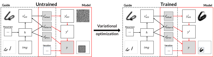
Figure 7. AIR is a generative model for multi-object images, trained with variational inference. The model randomly selects a number of patches to render onto a canvas, and a location, scale, and latent code for each. The variational family predicts these latent variables from an image. The model is trained on a dataset of images constructed by randomly translating and scaling MNIST digits onto a canvas.

AIR figure.

Table 2. Time (in seconds) to train the AIR model (Eslami et al., 2016) for one epoch (batch size 64) with different objectives and estimators. All discrete variables use the same estimation strategy. IWELBO runs have $n=2$ particles.

System	Compiler	REINFORCE	ENUM	MVD	IWELBO + REINFORCE	IWELBO + MVD
genjax.vi	JAX (XLA)	1.52 $\pm$ 0.05	6.22 $\pm$ 0.29	1.74 $\pm$ 0.04	2.28 $\pm$ 0.12	3.74 $\pm$ 0.05
pyro	Torch	12.28 $\pm$ 0.55	122.93 $\pm$ 1.74	X	22.17 $\pm$ 1.2	X

Expressivity and Compositional Correctness.

In Table 8, we enumerate several possible combinations of gradient estimation strategies and objectives for the AIR model. In Table 8, we consider the model shown in Fig. 2, and implement the model and naive variational guide in genjax.vi, Pyro and NumPyro, as well as the auxiliary variable variational guide in genjax.vi. We show statistics on final mean objective values for different variational objectives. While ELBO and IWELBO are standard, our system allows using more expressive approximations and tighter lower bound objectives compositionally (such as DIWHVI (Sobolev and Vetrov, 2019), which uses SIR to estimate densities of marginals, in the IWELBO objective) to achieve tighter variational bounds.

Figure 8. Combinatorial space of gradient estimators and objective functions for the AIR model, which our programmable approach helps to explore.

RE = REINFORCE estimator, EN = enumeration estimator, BL = REINFORCE with learned baselines, MV = measure-valued derivative estimator Grad. Estimation Strategies Objective Batch System RE. EN. BL. MV. Pyro Ours $\checkmark$ ELBO $\geq$ 1 $\checkmark$ $\checkmark$ 5-8 IWAE $\geq$ 1 $\checkmark$ $\checkmark$ 5-8 $\checkmark$ ELBO $\geq$ 1 $\checkmark$ $\checkmark$ 5-8 IWAE $\geq$ 1 $\times$ $\checkmark$ 5-8 $\checkmark$ ELBO $\geq$ 1 $\checkmark$ $\checkmark$ 5-8 IWAE $\geq$ 1 $\times$ $\checkmark$ 5-8 $\checkmark$ ELBO $\geq$ 1 $\times$ $\checkmark$ 5-8 IWAE $\geq$ 1 $\times$ $\checkmark$ 5-8 $\checkmark$ $\checkmark$ ELBO $\geq$ 1 $\checkmark$ $\checkmark$ 5-8 IWAE $\geq$ 1 $\times$ $\checkmark$ 5-8 $\checkmark$ $\checkmark$ ELBO $\geq$ 1 $\checkmark$ $\checkmark$ 5-8 IWAE $\geq$ 1 $\times$ $\checkmark$ 5-8 $\checkmark$ $\checkmark$ ELBO $\geq$ 1 $\times$ $\checkmark$ 5-8 IWAE $\geq$ 1 $\times$ $\checkmark$ 5-8 $\checkmark$ $\checkmark$ ELBO $\geq$ 1 $\times$ $\checkmark$ 5-8 IWAE $\geq$ 1 $\times$ $\checkmark$ 5-8 $\checkmark$ $\checkmark$ ELBO $\geq$ 1 $\times$ $\checkmark$ 5-8 IWAE $\geq$ 1 $\times$ $\checkmark$ 5-8 $\checkmark$ $\checkmark$ ELBO $\geq$ 1 $\times$ $\checkmark$ 5-8 IWAE $\geq$ 1 $\times$ $\checkmark$ 5-8 $\checkmark$ $\checkmark$ $\checkmark$ ELBO $\geq$ 1 $\times$ $\checkmark$ 5-8 IWAE $\geq$ 1 $\times$ $\checkmark$ 5-8 $\checkmark$ $\checkmark$ $\checkmark$ ELBO $\geq$ 1 $\times$ $\checkmark$ 5-8 IWAE $\geq$ 1 $\times$ $\checkmark$ 5-8 $\checkmark$ $\checkmark$ $\checkmark$ ELBO $\geq$ 1 $\times$ $\checkmark$ 5-8 IWAE $\geq$ 1 $\times$ $\checkmark$ 5-8 $\checkmark$ $\checkmark$ $\checkmark$ ELBO $\geq$ 1 $\times$ $\checkmark$ 5-8 IWAE $\geq$ 1 $\times$ $\checkmark$ 5-8         Not Exploited RWS 1 $\checkmark$ $\checkmark$ 6-8 $>$ 1 $\times$ $\checkmark$ 6-8 Figure 9. We evaluate a variety of custom estimators and objectives (ELBO, IWAE, RWS) using our system. Our on average best estimator (IWAE + MVD, not expressible in Pyro) converges an order of magnitude faster than Pyro’s recommended estimator.

Table 3. Mean objective value (in nats) on repeated runs for several variational objectives, including ones which utilize marginal. $n$ and $m$ denote particle sizes for SIR algorithms.

System	ELBO	IWELBO ($n=5$)	HVI	IWHVI ($m=5$)	DIWHVI ($n=5,m=5$)
genjax.vi	-8.08	-7.79	-9.75	-8.18	-7.33
numpyro	-8.08	-7.77	✓/ X	X	X
pyro	-8.08	-7.75	✓/ X	X	X

9. Related work

Variational Inference in PPLs.

Many PPLs support some form of variational inference (Bingham et al., 2019; Stites et al., 2021; Carpenter et al., 2017; Ge et al., 2018; Cusumano-Towner et al., 2019), and it is the primary focus of Pyro (Bingham et al., 2019) and ProbTorch (Stites et al., 2021). Both Pyro and ProbTorch have endeavored to make inference more programmable. For example, ProbTorch has introduced inference combinators that make it easy to express certain nested variational inference algorithms (Zimmermann et al., 2021; Stites et al., 2021). Pyro has perhaps the most mature support for variational inference, with many gradient estimators and objectives supported. Pyro also implements some variance reduction strategies not yet supported by our system, e.g. exploiting conditional independence using their plate operator. However, extending Pyro with new variational objectives or gradient estimation strategies requires a deep understanding of its internals. Furthermore, Pyro’s modeling language does not have our constructs for marginalization and normalization (although Pyro can marginalize discrete, finite-support auxiliary variables from models). Concurrently with this work, Wagner (2023) presented a PPL with correct-by-construction variational inference, where their notion of “correctness” is stronger in some ways and weaker in others than that of this work. In particular, Wagner (2023) works with smoothed approximations of the user’s probabilistic programs, and so the gradient estimates it computes are biased for the original objective. However, the degree of error in this smoothing is gradually annealed over the course of optimization, leading to convergence to a stationary point of the original objective.

Static Analyses for Differentiability Criteria.

Within the PL community, researchers have made some progress toward formalizing and developing static analyses for ensuring soundness properties of variational inference (Lee et al., 2019, 2023; Wang et al., 2021), as well as program transformations for automatically constructing variational families informed by the model’s structure (Li et al., 2023b). By contrast, we formalize the process by which user model, inference, and objective code is transformed into a gradient estimator, tracking the interactions between density computation, simulation, and automatic differentiation. One interesting direction would be to extend Lee et al. (2023)’s analysis to automatically annotate $\lambda_{\text{Gen}}$ programs with gradient estimators. Note that our current type-based analysis does not verify the local domination condition of Thm. 5.2, which Wagner (2023) does manage to check statically, by imposing restrictions on the PPL and considering only the ELBO objective.

Automated Gradient Estimation.

Due to its centrality to many applications in computer science and beyond, there has been intense interest in automating unbiased gradient estimation for objective functions expressed as expectations, yielding several frameworks for unbiasedly differentiating first-order stochastic computation graphs (Krieken et al., 2021; Schulman et al., 2015; Weber et al., 2019), imperative programs with discrete randomness (Arya et al., 2022), and higher-order probabilistic programs (Lew et al., 2023b). Some works have also investigated automated computation of biased gradient estimates via smoothing (Kreikemeyer and Andelfinger, 2023). However, these frameworks cannot be directly applied to variational inference problems, which require differentiating not just user code, but also traced simulators and log density evaluators of the probabilistic programs that users write. We address these challenges, by compiling density functions of user-defined probabilistic programs into a target language compatible with ADEV (Lew et al., 2023b). We also extend ADEV in several other ways: our version adds score to differentiate not just expected values but general integrals against (potentially unnormalized) measures; is implemented performantly on GPU; and has been extended with a reverse-mode.

Programmable Inference.

We build on a long line of work that aims to make inference more programmable in PPLs (Mansinghka et al., 2014, 2018; Narayanan et al., 2016; Cusumano-Towner et al., 2019; Lew et al., 2023a). In much the same way that this prior work has aimed to expose compositional structure in Monte Carlo algorithms and help users explore a broad class of algorithm settings, our work aims to do the same for variational inference, exposing compositional structure in gradient estimators and variational objectives.

Formal Reasoning about Inference and Program Transformations.

Our semantics builds on recent work in the denotational semantics and validation of Bayesian inference (Ścibior et al., 2017; Heunen et al., 2017; Ścibior et al., 2018), as well as semantic foundations for differentiable programming (Huot et al., 2020; Sherman et al., 2021). Our soundness proofs are based on logical relations (Ahmed, 2006; Huot et al., 2020). We also draw on a tradition of deriving probabilistic inference algorithms via program transformations (Narayanan et al., 2016).

10. Discussion

This work gives a formal account of the automation that PPLs provide for variational inference — a powerful and widely used suite of features that has not previously been completely understood in formal programming language terms. This work’s account provides a careful separation of the interactions between tracing, density computation, gradient estimation strategies, and automatic differentiation. Simultaneously, this work shows how to implement these features modularly and extensibly, addressing a number of pain points in existing implementations, and expanding the class of variational inference algorithms that users can easily express.

Limitations.

That said, the modular approach we have presented has several key limitations:

• Static checks may be unnecessarily restrictive. For example, although the rectified linear unit (ReLU) is not differentiable at 0, in many (but not all) contexts it is safe to use it as though it were differentiable, without compromising unbiasedness. The type system of $\lambda_{\text{ADEV}}$ is not sophisticated enough to distinguish when ReLU is safe or not, and so we must give it the restrictive type $\mathbb{R}^{*}\rightarrow\mathbb{R}^{*}$. Of course, at their own risk, users of the system are free to ignore these static checks.

• No parametric discontinuities. A key limitation of our language, shared by Pyro, ProbTorch, and Gen, is that parametric discontinuities (expressions that compute discontinuous functions of the input parameters) are not permitted. Variational inference is possible in these settings, and Lee et al. (2018) proposed a gradient estimator that can be automated for a restricted PPL with affine discontinuities. More recently, Bangaru et al. (2021) and Michel et al. (2024) have presented techniques for differentiating integral expressions with parametric discontinuities. It is not yet clear to what extent the design we present could be cleanly extended to exploit these techniques.

• User-specified variational objectives may be ill-defined. Our correctness theorem assumes as a precondition that the objective the user has specified is well-defined (i.e., if it is defined as an expected value, that it is finite for all input parameters). Previous work has identified the verification of this condition as an important challenge for safe variational inference (Lee et al., 2019), but our system includes no static checks to do so.

• Continuation-passing style (CPS) is unnatural in many host languages. $\textbf{adev}\{\cdot\}$ transforms a program to CPS in order to automate unbiased gradient estimation. This is easy in our Haskell implementation, but in Python and Julia, it introduces some amount of friction. For example, in Julia, certain host-language features (like mutation, and therefore most imperative loops) are incompatible with our CPS implementation. By contrast, Pyro and Gen place few restrictions on the host-language features that can be used to define models and variational families.

In addition, our implementation does not yet incorporate several important insights and capabilities from existing deep PPLs, including Pyro’s use of tensor contractions to marginalize discrete variables (Obermeyer et al., 2019a, b), or the use of fine-grained control flow information to reduce the variance of gradient estimates (Schulman et al., 2015).

Future Work.

We comment on several intriguing avenues for future work:

• The search for low variance estimators. Our approach automates the derivation of unbiased gradient estimators, but it says little about what estimators one should choose to achieve low variance on particular problems. Our approach should make it easier to address this challenge, by allowing rapid exploration of a large space of estimation strategies, some of which have not been previously automated. We hope that our work and implementations might be used to carry out a study of the behavior of different gradient estimators, on a broader variety of problems than those enabled by current automation.

• Interaction with ADEV. Our system is the first to use ADEV (Lew et al., 2023b) for scalable learning of large parameter spaces (§A.4). ADEV provides a fundamentally new perspective on automatic differentiation, and extends the technique to expected value loss functions. Our integration with ADEV has several implications: by virtue of the fact that the target language of our language’s transformations is ADEV’s source language, our system may be used with ADEV loss functions beyond the variational loss functions which we’ve discussed in this work. Extensions to ADEV which improve variance properties of gradient estimators symbiotically improve the performance of gradient estimators in our language. Indeed, we expect new investigations into low variance gradient estimators for discrete random choices (Arya et al., 2022) to open up novel variational guide families, hitherto unexplored due to poor variance or computational intractability of discrete enumeration.

Data-Availability Statement

An artifact providing a version of genjax.vi, and reproducing our experiments, is available (Becker et al., 2024).

Appendix A Full Language and System

We elaborate on our discussion in §7, and provide a sketch of the changes that would be necessary to adapt our formal model and proofs to the generative language extended with marginal and normalize, and the reverse mode implementation of ADEV.

A.1. New Language Features for Expressive Models and Variational Families

The full language for models and variational families modularly extends our formalized core with two new constructs: marginal, for marginalizing auxiliary variables from the model or variational family; and normalize, for building variational families that use Monte Carlo to approximate the normalized posteriors of other programs. We discuss each feature in turn.

Marginalization of auxiliary variables. A key requirement in variational inference is that the model and variational family be defined over the same set of random variables (Lee et al., 2019; Lew et al., 2019; Wang et al., 2021; Li et al., 2023b). But it is often desirable to introduce auxiliary variables to only the variational family, or only the model, in order to make the marginal distribution on the shared variables more interesting. Fig. 2 illustrates one example. Both the model and variational family are defined over $x$ and $y$, and intuitively, we want the variational family to learn a distribution that concentrates mass around the circumference of a circle of radius $\sqrt{5}$. But using Gaussian primitives alone we can never express such a distribution. Therefore, guide_joint introduces an auxiliary variable $v\sim U([0,2\pi])$, which informs the location of both $x$ and $y$. Because guide_joint is now defined over the three variables $(v,x,y)$, it is no longer directly usable as a variational family for the model. Using marginal, we can fix the problem, constructing a new program representing guide_joint’s marginal on $x$ and $y$.

The syntax for marginalizing is marginal names program algorithm. The argument names is a list of strings indicating which of the variables from program should be kept. Marginal distributions may have intractable density functions, and so our system automates differentiable stochastic estimates of their densities instead (§A.2). The argument algorithm specifies a strategy for calculating these estimates. It is given as a function, taking in values for the variables in names, and outputting an algorithm for inferring the posterior over auxiliary variables (see §A.2 for details).

Usage. With marginal, users can encode within a PPL many variational inference algorithms that cannot be easily expressed in existing systems. For example, hierarchical variational inference (HVI) (Ranganath et al., 2016; Agakov and Barber, 2004) can be implemented by introducing then marginalizing auxiliary variables in a variational family, using 1-particle importance sampling as the algorithm argument. Increasing the number of particles used to estimate the marginal density of the variational family yields importance-weighted HVI (Sobolev and Vetrov, 2019). Parameterizing the proposal used to marginalize the variational family as a neural network recovers auxiliary deep generative models (ADGM) (Maaløe et al., 2016). Nesting a marginal distribution as the proposal to marginalize a variational family is an instance of recursive auxiliary-variable inference (RAVI) (Lew et al., 2022). Extending the variational family with steps from a Markov chain Monte Carlo algorithm, then marginalizing those, implements Markov chain variational inference (MCVI) (Salimans et al., 2015). And many aspects of these algorithms could in principle be composed to develop new inference algorithms altogether.

Approximate normalization. Another way to make variational families more expressive is to add general-purpose inference logic to the variational family itself. To do this, users can apply our normalize construct, which builds a probabilistic program that represents the output distribution of a given inference algorithm applied to a given (unnormalized) probabilistic program. Its syntax is normalize program algorithm.

Usage. Fig. 3 illustrates a typical usage: after defining a simple variational family ($\texttt{q}_{\texttt{NAIVE}}$), we define an improved variational family ($\texttt{q}_{\texttt{SIR}}$) that performs $N$-particle importance sampling, targeting the model’s posterior, using $\texttt{q}_{\texttt{NAIVE}}$ as a proposal distribution. This normalized variational family can then be used in several ways. If we use $\texttt{q}_{\texttt{SIR}}$ as a variational family and optimize the usual ELBO objective (using our stochastically estimated densities for $\texttt{q}_{\texttt{SIR}}$, see §A.2), this is equivalent to optimizing the IWAE (or IWELBO) objective with $\texttt{q}_{\texttt{NAIVE}}$ as the variational family (Burda et al., 2016). Alternatively, we can optimize the objective $\phi\mapsto\mathbb{E}_{x\sim\llbracket\texttt{q}_{\texttt{SIR}}{\phi_{0}}\rrbracket}[-\log~{}\llbracket\textbf{density}\{\texttt{q}_{\texttt{NAIVE}}\}\rrbracket_{\phi}(x)]$, which tunes $\texttt{q}_{\texttt{NAIVE}}$ to minimize its KL divergence to the approximate inference algorithm $\texttt{q}_{\texttt{SIR}}$. This latter objective is the wake-phase $\phi$ objective in the reweighted wake sleep algorithm (Bornschein and Bengio, 2015; Le et al., 2019), and is illustrated as a $\lambda_{\text{ADEV}}$ program in §B.

A.2. Differentiable Stochastic Estimators of Densities and their Reciprocals

With the new features from §A.1, it is possible to define models and variational families whose exact densities cannot be efficiently computed. As such, in our full language, density and sim do not produce exact density evaluators, but rather density estimators that may be stochastic, depending on the input program. Importantly, these estimators are still implemented in the ADEV language, still come equipped with gradient estimation strategies, and are still guaranteed to satisfy the necessary differentiability requirements for gradients to be unbiased. We now discuss the implications of this stochastic estimation for users of our language; see § A.3 for an overview of how the stochastic estimates are computed.

For users. On the surface, very little changes when densities are made stochastic. The automated density procedures now have type $\text{Trace}\to P~{}\mathbb{R}$, instead of $\text{Trace}\to\mathbb{R}$, and the specifications for both density and sim change slightly: now, $\textbf{density}\{t\}$ produces only unbiased estimates of the density of $\llbracket t\rrbracket_{1}$, and $\textbf{sim}\{t\}$ produces pairs $(x,w)$ with the property that $\mathbb{E}[\frac{1}{w}\mid x]$ is the reciprocal density of $\llbracket t\rrbracket_{1}$ at $x$. But using density estimators instead of exact densities can change the meaning of user-specified variational objectives. Consider, for example, the ELBO, whose implementation is very slightly modified to account for the new type of density: ELBO≔λ(θ, ϕ). E(do {(x, w_q)←sim{Q}  ϕ; w_p←density{P}  θ x; returnlogw_p - logw_q}).

This program may no longer denote the usual ELBO objective, $\int\log\frac{\tilde{p}_{\theta}(x)}{q_{\phi}(x)}\ \ Q_{\phi}(x)dx.$ Instead, it denotes the objective (θ, ϕ) ↦∬logwpwq κ_p;θ(x, dw_p)κ_q;ϕ(dx, dw_q), where we write $\kappa_{p}$ for the unbiased density estimation kernel for $P_{\theta}$ (the new specification for $\mathbf{density}\{t_{p}\}$) and $\kappa_{q}$ for the ‘reciprocal density simulation’ measure for $Q_{\phi}$ (the new specification for $\mathbf{sim}\{t_{q}\}$). Fortunately, however, this is still a sensible variational objective. Because $\mathbb{E}[w_{p}\mid x]=\tilde{p}_{\theta}(x)$ and $\mathbb{E}[\frac{1}{w_{q}}\mid x]=\frac{1}{q_{\phi}(x)}$, we can apply Jensen’s inequality and obtain that $\mathbb{E}[\log w_{p}\mid x]\leq\log\tilde{p}_{\theta}(x)$ and $\mathbb{E}[\log\frac{1}{w_{q}}\mid x]\leq\log\frac{1}{q_{\phi}(x)}$. This in turn implies that our new objective is a lower bound on the original ELBO. In fact, it can be shown that the new bound decomposes as the original ELBO plus a non-negative term related to the average variation of the stochastic density estimates (Lew et al., 2022). Thus, optimizing this modified ELBO simultaneously maximizes the original ELBO and minimizes the variability of the density estimates.

A.3. Estimator implementation

To implement density estimation, we take inspiration from (Lew et al., 2023a). We first extend our language with a new type for inference algorithms; currently we have implemented only importance-sampling algorithms, constructed with the syntax $\textbf{importance}~{}\textit{proposal}~{}N$. The $\xi$ and $\chi$ transformations from §4 are then extended to transform importance-sampling algorithms into ADEV-compatible procedures for, given an unnormalized model of type $G~{}\tau$, (1) generating collections of importance-weighted particles from the proposal, and (2) given a sample $x$, generating collections of conditional importance samples (at least one of which is equal to $x$) (Cusumano-Towner and Mansinghka, 2017; Naesseth et al., 2019). The importance sampling is implemented in terms of the proposal’s sim method and the model’s density method, so any gradient estimation logic is incorporated into the generated ADEV procedures. The marginal and normalize constructs expect algorithms as inputs, which they use as follows to estimate their densities and density reciprocals:

• To implement density for marginal names prog alg, we first construct an unnormalized posterior over auxiliary variables to marginalize by transforming prog to observe all random variables in names. We then estimate its normalizing constant—the marginal density of the observed choices—by generating (unconditional) importance samples from alg and averaging the importance weights. For sim, we simulate a complete trace $t$ from prog and project out the variables from names to obtain a marginal sample. We then proceed as before to estimate the density, but use conditional importance samples, conditioned on the auxiliary variables sampled when generating $t$. This can be shown to have the desired unbiasedness property (Lew et al., 2023a).

• To implement density for normalize prog alg for a given trace $t$, we first call $\textbf{density}\{\textit{prog}\}$ on $t$ to get its unnormalized density. We then use conditional importance sampling (conditioned on $t$ using alg targeting prog, and compute the average weight. The ratio of the unnormalized density to the average weight is an unbiased estimate of the output density of sampling-importance-resampling (SIR) (Rubin, 1988) at $t$. To implement sim, we draw unconditional importance samples, and resample one from a categorical distribution based on the importance weights. We then call $\textbf{density}\{\textit{prog}\}$ on the chosen trace $t$ and return $(t,w)$, where $w$ is the ratio of the chosen trace’s unnormalized density to the average importance weight. The categorical sample needs a gradient estimator—we use $\textbf{categorical}_{\text{ENUM}}$.

A.4. Reverse-Mode Automatic Differentiation of Expected Values

The algorithm we present in §6 is a forward-mode AD algorithm, which works by propagating dual numbers. Unfortunately, forward-mode algorithms do not scale to typical deep learning applications, because they can compute only one dimension of the gradient per execution. Our implementations extend ADEV to support reverse-mode, which can compute gradients in one pass:

• Our genjax.vi implementation is built on top of JAX, which takes a unique approach to reverse-mode for deterministic programs (Radul et al., 2022) (YOLO). It involves first applying a forward-mode program transformation, then separating the transformed program into linear and non-linear components, and finally transposing the linear component via another program transformation. This is a powerful technique that avoids the need to write a specialized reverse-mode algorithm, but only applies to first-order deterministic programs, which at first glance rules out ADEV’s reliance on higher-order continuation-passing style and on random sampling. The first restriction can be lifted by partial evaluation: if we begin with a first-order user program in genjax.vi — after apply ADEV’s transformations — we can $\beta$-reduce away (via JAX’s partial evaluation) any higher-order subterms introduced by the CPS transformation, allowing us to take first-order programs to first-order programs. Following YOLO, we then apply the unzip transformation $\mathcal{U}$, and the transposition transformation $\mathcal{T}$ to the deterministic parts of the resulting first-order programs. The restriction on random sampling can be lifted by the observation that sampling can be safely included in the nonlinear fragment of YOLO’s language – meaning that it is safe to extend YOLO with ADEV sampling primitives, so long as they implement gradient strategies that do not introduce sampling statements which depend on the linear tangent perturbations. We exemplify the process of using YOLO’s transformations to derive a reverse mode gradient estimator in Fig. 10.

• In Julia and Haskell, we take a different approach. We begin with existing libraries for deterministic, reverse-mode AD, and attempt to transform the user’s program into a host-language program that, when standard reverse-mode AD is applied, will yield a correct gradient estimator. To achieve this, we still apply a continuation-passing transformation to the user’s program, and replace stochastic primitives with special CPS-style gradient estimators. But we must write the primitives so that, instead of stochastically returning manually constructed dual numbers, they stochastically return scalar losses whose reverse-mode derivatives are as desired. To achieve this, we use phony “functions” analogous to the “magic-box” operators in DICE (Foerster et al., 2018) or Storchastic (Krieken et al., 2021), which introduce phantom dependencies on scalars so that their derivatives will include extra terms. This sort of trick is widely used to implement gradient estimators without giving up on deterministic AD’s benefit; what is nice about combining the trick with ADEV is that (1) the hacky use of phony functions is limited to the implementations of primitives, which still have local specifications that can be separately reasoned about; and (2) we still benefit from the expressive power of ADEV’s continuations, which can express gradient estimators that require much more substantial changes to the original program than simply tracking a few extra gradient terms.

(a) Input Loss as a	(b) Apply Forward-mode	(c) Inline $\mathcal{D}\{\mathbf{\color[rgb]{0,0,0.7}{\mathbb{E}}}\},\mathcal{D}\{\mathbf{\color[rgb]{0,0,0.7}{normal_{\texttt{REPARAM}}}}\}$
Probabilistic Program	ADEV $\mathcal{D}\{-\}$	and $\beta$-reduce $\lambda$’s
$\mathcal{L}=\lambda(\otimes\underline{\theta};):\mathbb{R}^{2}.\,\mathbf{\color[rgb]{0,0,0.7}{\mathbb{E}}}(\textbf{do}~{}\{$ $\quad\textbf{let}\ (x;)\leftarrow\mathbf{\color[rgb]{0,0,0.7}{normal_{\texttt{REPARAM}}}}(\underline{\theta}_{1},1)$ $\quad\textbf{let}\ (y;)=\sin(x)$ $\quad\textbf{let}\ (z;)=y+\underline{\theta}_{2}$ $\quad\quad\textbf{return}~{}z\})$	$d\mathcal{L}=\lambda(\otimes\underline{\theta};\otimes\underline{\dot{\theta}}):\mathbb{R}^{2}\times\mathbb{R}^{2}.\,\mathcal{D}\{\mathbf{\color[rgb]{0,0,0.7}{\mathbb{E}}}\}$ $\big{(}\lambda dl.\textbf{do}~{}\{$ $\quad\mathcal{D}\{\mathbf{\color[rgb]{0,0,0.7}{normal_{\texttt{REPARAM}}}}\}\big{(}(\underline{\theta}_{1},1),(\underline{\dot{\theta}}_{1},0)\big{)}$ $\quad\big{(}\lambda(x;\dot{x}).$ $\quad\quad\textbf{let}\ (y;)=\sin(x)$ $\quad\quad\textbf{let}\ (dy;)=\cos(x)$ $\quad\quad\textbf{let}\ (;\dot{y})=dy*\dot{x}$ $\quad\quad\textbf{let}\ (z;)=y+\underline{\theta}_{2}$ $\quad\quad\textbf{let}\ (;\dot{z})=\dot{y}+\underline{\dot{\theta}}_{2}$ $\quad\quad\quad dl(z,\dot{z})\big{)}\}\big{)}$	$d\mathcal{L}=\lambda(\otimes\underline{\theta};\otimes\underline{\dot{\theta}}):\mathbb{R}^{2}\times\mathbb{R}^{2}.\,\textbf{do}~{}\{$ $\quad\textbf{let}\ (\epsilon;)\leftarrow\mathbf{\color[rgb]{0,0,0.7}{normal_{\texttt{REPARAM}}}}(0,1)$ $\quad\textbf{let}\ (x_{1};)=\epsilon*1$ $\quad\textbf{let}\ (;\dot{x_{1}})=\epsilon*0$ $\quad\textbf{let}\ (x;)=x_{1}+\underline{\theta}_{1}$ $\quad\textbf{let}\ (;\dot{x})=\dot{x_{1}}+\underline{\dot{\theta}}_{1}$ $\quad\textbf{let}\ (y;)=\sin(x)$ $\quad\textbf{let}\ (dy;)=\cos(x)$ $\quad\textbf{let}\ (;\dot{y})=dy*\dot{x}$ $\quad\textbf{let}\ (z;)=y+\underline{\theta}_{2}$ $\quad\textbf{let}\ (;\dot{z})=\dot{y}+\underline{\dot{\theta}}_{2}$ $\quad\quad\textbf{return}(z,\dot{z})\}$

(d) Apply Unzip macro	(e) Apply Transpose on linear part	(f) Simplify and initialise reverse-mode
$d\mathcal{L}.nonlin=\lambda(\otimes\underline{\theta};):\mathbb{R}^{2}.\,\textbf{do}~{}\{$ $\quad\textbf{let}\ (\epsilon;)\leftarrow\mathbf{\color[rgb]{0,0,0.7}{normal_{\texttt{REPARAM}}}}(0,1)$ $\quad\textbf{let}\ (x_{1};)=\epsilon*1$ $\quad\textbf{let}\ (x;)=x_{1}+\underline{\theta}_{1}$ $\quad\textbf{let}\ (y;)=\sin(x)$ $\quad\textbf{let}\ (dy;)=\cos(x)$ $\quad\textbf{let}\ (z;)=y+\underline{\theta}_{2}$ $\quad\textbf{let}\ (\underline{trace};)=\otimes(\epsilon,x_{1},x,y,dy,z)$ $\quad\quad\textbf{return}(z,trace)\big{)}$ $d\mathcal{L}.lin=\lambda(\otimes\underline{trace};\otimes\underline{\dot{\theta}}):\otimes\mathbb{R}\times\mathbb{R}^{2}.\,$ $\quad\textbf{let}\ (\epsilon,x_{1},x,y,dy,z;)=\underline{trace}$ $\quad\textbf{let}\ (;\dot{x_{1}})=\epsilon*0$ $\quad\textbf{let}\ (;\dot{x})=\dot{x_{1}}+\underline{\dot{\theta}}_{1}$ $\quad\textbf{let}\ (;\dot{y})=dy*\dot{x}$ $\quad\textbf{let}\ (;\dot{z})=\dot{y}+\underline{\dot{\theta}}_{2}$ $\quad\quad\textbf{return}\ \dot{z}$	$d\mathcal{L}.nonlin=\lambda(\otimes\underline{\theta};):\mathbb{R}^{2}.\,\textbf{do}~{}\{$ $\quad\textbf{let}\ (\epsilon;)\leftarrow\mathbf{\color[rgb]{0,0,0.7}{normal_{\texttt{REPARAM}}}}(0,1)$ $\quad\textbf{let}\ (x_{1};)=\epsilon*1$ $\quad\textbf{let}\ (x;)=x_{1}+\underline{\theta}_{1}$ $\quad\textbf{let}\ (y;)=\sin(x)$ $\quad\textbf{let}\ (dy;)=\cos(x)$ $\quad\textbf{let}\ (z;)=y+\underline{\theta}_{2}$ $\quad\textbf{let}\ (\underline{trace};)=\otimes(dy)$ $\quad\quad\textbf{return}(z,\underline{trace})\big{)}$ $d\mathcal{L}.lin=\lambda(\otimes\underline{trace};\dot{z}):\otimes\mathbb{R}\times\mathbb{R}.\,$ $\quad\textbf{let}\ (dy;)=\underline{trace}$ $\quad\textbf{let}\ (;\dot{y})=\dot{z}$ $\quad\textbf{let}\ (;\underline{\dot{\theta}}_{2})=\dot{z}$ $\quad\textbf{let}\ (;\dot{x})=dy*\dot{y}$ $\quad\textbf{let}\ (;\dot{x_{1}})=\dot{x}$ $\quad\textbf{let}\ (;\underline{\dot{\theta}}_{1})=\dot{x}$ $\quad\quad\textbf{return}\ \underline{\dot{\theta}}$	$d\mathcal{L}.nonlin=\lambda(\otimes\underline{\theta};):\mathbb{R}^{2}.\,\textbf{do}~{}\{$ $\quad\textbf{let}\ (\epsilon;)\leftarrow\mathbf{\color[rgb]{0,0,0.7}{normal_{\texttt{REPARAM}}}}(0,1)$ $\quad\textbf{let}\ (x;)=\epsilon+\underline{\theta}_{1}$ $\quad\textbf{let}\ (y;)=\sin(x)$ $\quad\textbf{let}\ (dy;)=\cos(x)$ $\quad\textbf{let}\ (z;)=y+\underline{\theta}_{2}$ $\quad\textbf{let}\ (\underline{trace};)=\otimes(dy)$ $\quad\quad\textbf{return}(z,\underline{trace})\big{)}$ $d\mathcal{L}.grad=\lambda(\otimes\underline{trace};):\otimes\mathbb{R}.\,$ $\quad\textbf{let}\ (dy;)=\underline{trace}$ $\quad\textbf{let}\ (;\underline{\dot{\theta}}_{2})=1$ $\quad\textbf{let}\ (;\underline{\dot{\theta}}_{1})=dy$ $\quad\quad\textbf{return}\ \underline{\dot{\theta}}$

Figure 10. Deriving a reverse mode gradient estimator for a program in $\lambda_{\text{ADEV}}$ via YOLO (Radul et al., 2022). We’ve dropped $\mathbf{\color[rgb]{0,0,0.7}{in}}$ for readability.

Appendix B Additional Variational Objectives in $\lambda_{\text{ADEV}}$

IWELBO, IWHVI, and DIWHVI are all objectives which are based on evidence lower bounds. Many variational algorithms also make use of objectives motivated by the forward KL divergence

$$\mathcal{F}_{\text{KL}(P,Q)}:=\mathbb{E}_{z\sim P}[\log\frac{\textbf{density}\{P\}(z)}{\textbf{density}\{Q\}(z)}]$$

where, for instance, $Q$ has learnable parameters and $P$ is taken to be a posterior. $P$ may be intractable — we may not have access to simulators or density evaluators for $P$. In this setting, several variational algorithms (Hinton et al., 1995; Bornschein and Bengio, 2015; Gu et al., 2015) consider a modified objective where inference is used to approximate $P$ — these algorithms utilize $Q$ as part of the Alg approximation:

$$\mathcal{F}_{\text{KL}(\text{Alg}(Q),Q)}:=\mathbb{E}_{z\sim\text{Alg}(Q)}[\log\frac{\textbf{density}\{\text{Alg}(Q)\}(z)}{\textbf{density}\{Q\}(z)}]$$

Of course, for a fixed Alg, the estimators constructed from the modified objective will be biased estimators of the original forward KL objective — where the bias is controlled by the accuracy of the approximation of $P$ induced by Alg. Importantly, our language includes the possibility of using these objectives in variational algorithms: for instance, the wake phase $Q$-update gradient estimator from (Bornschein and Bengio, 2015) can be derived in $\lambda_{\text{ADEV}}$ (plus our full system extensions for estimated densities) from the objective:

$\textbf{QWake}(N,P,Q,\phi^{\prime})\coloneqq\lambda\phi.\mathbb{E}(\textbf{do}~{}\{$ $\quad\quad(z,\_)\leftarrow\textbf{sim}\{\lambda\phi^{\prime}.\textbf{normalize}\ P\ (\textbf{importance}\ (Q\ \phi^{\prime})\ N)\}~{}\phi^{\prime};$ $\quad\quad q\leftarrow(\textbf{density}\{Q\}~{}\phi)~{}z;$ $\quad\quad\textbf{return}-log~{}q$ $\})$

and also, the wake-phase $P$-update:

$\textbf{PWake}(N,P,Q,\phi^{\prime})\coloneqq\lambda\theta.\mathbb{E}(\textbf{do}~{}\{$ $\quad\quad(z,w_{q})\leftarrow\textbf{sim}\{\lambda\theta.\textbf{normalize}\ (P\ \theta)\ (\textbf{importance}\ (Q\ \phi^{\prime})\ N)\}~{}\theta;$ $\quad\quad p\leftarrow(\textbf{density}\{P\}~{}\theta)~{}z;$ $\quad\quad\textbf{return}~{}(log~{}p)-(log~{}w_{q})$ $\})$

where, in this objective, $P$ is a term of type $\mathbb{R}^{M}\rightarrow D\ \tau$. Indeed, this allows one to implement learning architectures like reweighted wake-sleep (Bornschein and Bengio, 2015) in $\lambda_{\text{ADEV}}$.

Appendix C Evaluation: Hand Coded Program vs. Our Implementation

In §8 and Table 1, we provided evaluation time comparisons between gradient estimators for the ELBO of a variational autoencoder derived using our system and a manually coded implementation. Below, we illustrate the programs used to construct this comparison, and runtime curves as a function of batch size.

Hand coded gradient estimator ⬇ def vae_reparam_loss(key, params): (encoder, decoder) = params loc, diag_scale = encoder(image) v = mv_normal_sample(key, zeros(10), ones(10)) s = loc + v * diag_scale guide_n_logp = mv_normal_log_prob( s, loc, diag_scale ) model_n_logp = mv_normal_log_prob( s, zeros(10), ones(10) ) logits = decoder(s) model_b_logp = bernoulli_log_prob(logits, image) return (model_b_logp.sum() + model_n_logp - guide_n_logp) \parkey = PRNGKey(314159) jax.grad(loss_estimate, argnums=1)(key, params)

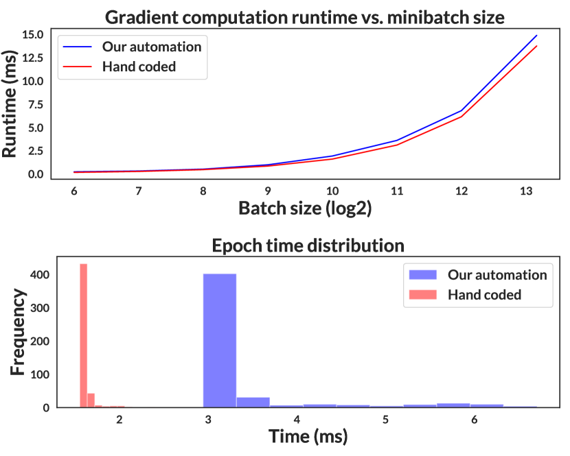
Model program ⬇ @genjax.gen def model(decoder): latent = genjax.vi.mv_normal_diag_reparam( zeros(10), ones(10) ) @ ”latent” logits = decoder(latent) genjax.vi.flip_reinforce(logits) @ ”image” Guide program ⬇ @genjax.gen def guide(encoder, chm): image = chm[”image”] loc, scale_diag = encoder(image) genjax.vi.mv_normal_diag_repram( loc, scale_diag ) @ ”latent”

Loss program (with automated estimator) ⬇ chm = genjax.choice_map({”image”: data}) \par@genjax.adev def elbo(decoder, encoder): (v, w_q) = guide.sim(encoder, chm) w_p = model.density(merge(v, chm), decoder) return log(w_p) - log(w_q) \parkey = PRNGKey(314159) elbo.grad_estimate(key, (decoder, encoder))

Figure 11. Comparing a hand coded VAE ELBO gradient estimator (top left) to our implementation. (Bottom) Our language and implementation supports a modular separation of gradient strategies, model and guide programs, and loss specification. (Top right) We investigate the runtime cost of our abstractions in a parallelization experiment (increasing batch size), and find a negligible impact on runtime performance.

Appendix D Evaluation: Additional Experiments

We performed additional experiments comparing genjax.vi to Pyro and NumPyro, on tutorial examples drawn from Pyro’s website. These examples include applying variational inference to a coin flip model, Bayesian linear regression, and semi-supervised and conditional variational autoencoders. In this section, we provide a discussion of the experiments and a selection of our results. For all experiments, we use the standard definition of ELBO in $\lambda_{\text{ADEV}}$: ELBO(P, Q) ≔λ(θ,ϕ). E(do {(x, w_q)←sim{Q}  ϕ; w_p←density{P} θ x; returnlogw_p - logw_q})

D.1. Fairness inference of a noisy coin

We consider a model over the latent fairness of a coin. We observe a sequence of coin flips of length $10$, and seek to infer the distribution over the fairness (the probability) of the coin flip, a Bernoulli random variable. The model and guide programs can be expressed in $\lambda_{\text{Gen}}$:

$\textbf{model}\coloneqq\lambda~{}flips.(\textbf{do}~{}\{$ $\quad\quad p\leftarrow\textbf{sample}~{}\textbf{beta}(10.0,10.0)~{}\text{"fairness"};$ $\quad\quad\textbf{mapM}~{}(\lambda x.~{}\textbf{observe}~{}\textbf{bernoulli}(p)~{}x)~{}flips$ $\})$ $\textbf{guide}\coloneqq\lambda\phi.(\textbf{do}~{}\{$ $\quad\quad\alpha=\pi_{1}~{}\phi;$ $\quad\quad\beta=\pi_{2}~{}\phi;$ $\quad\quad\_\leftarrow\textbf{sample}~{}\textbf{beta}_{\text{IMPLICIT}}(\alpha,\beta)$ ”fairness” $\})$

We train the guide using gradient estimators for the ELBO. We’ve summarized the results across the 3 systems in the table below, comparing the average time per epoch, the average of ELBO estimates on the last 100 training steps, and, taking the learned parameter values of the guide, the inferred posterior mean (given by $\mu=\frac{\alpha}{\alpha+\beta}$, where $\alpha$ and $\beta$ are the parameters to the beta sampler (above, $\pi_{1}~{}\phi$ and $\pi_{2}~{}\phi$)).

System	Average wall time per epoch	Average of ELBO estimates (last $100$ steps)	Inferred posterior mean
genjax.vi	0.97 (ms)	-7.06	$0.529\pm 0.09$
NumPyro	0.66 (ms)	-7.07	$0.531\pm 0.09$
Pyro	0.77 (ms)	-7.07	$0.532\pm 0.09$

D.2. Bayesian linear regression

We consider the linear regression model from Introduction to Pyro: the goal is to fit a regression model for the GDP of a country given a Boolean value (whether or not the country is in Africa) and a $\mathbb{R}$ value (the Terrain Ruggedness Index measurement of the country). The model and guide programs can be expressed in $\lambda_{\text{Gen}}$:

$\textbf{model}\coloneqq\lambda(gdps,cafrica,ruggedness).(\textbf{do}~{}\{$ $\quad\quad a\leftarrow\textbf{sample}~{}\textbf{normal}(0.0,10.0)~{}\text{"a"};$ $\quad\quad ba\leftarrow\textbf{sample}~{}\textbf{normal}(0.0,1.0)~{}\text{"bA"};$ $\quad\quad br\leftarrow\textbf{sample}~{}\textbf{normal}(0.0,1.0)~{}\text{"bR"};$ $\quad\quad bar\leftarrow\textbf{sample}~{}\textbf{normal}(0.0,1.0)~{}\text{"bAR"};$ $\quad\quad s\leftarrow\textbf{sample}~{}\textbf{uniform}(0.0,10.0)~{}\text{"sigma"};$ $\quad\quad m=(a+ba\times cafrica~{}+$ $\quad\quad\quad\quad\quad\quad br\times ruggedness~{}+$ $\quad\quad\quad\quad\quad\quad bar\times cafrica\times ruggedness);$ $\quad\quad\textbf{mapM}~{}(\lambda x.~{}\textbf{observe}~{}\textbf{normal}(m,s)~{}x)~{}gdps$ $\})$ $\textbf{guide}\coloneqq\lambda(\phi,cafrica,ruggedness).(\textbf{do}~{}\{$ $\quad\quad(al,as,wl0,ws0,wl0,ws1,wl1,ws2,wl2,sl)=\phi;$ $\quad\quad a\leftarrow\textbf{sample}~{}\textbf{normal}_{\text{REPARAM}}(al,as)~{}\text{"a"};$ $\quad\quad ba\leftarrow\textbf{sample}~{}\textbf{normal}_{\text{REPARAM}}(wl0,ws0)~{}\text{"bA"};$ $\quad\quad br\leftarrow\textbf{sample}~{}\textbf{normal}_{\text{REPARAM}}(wl1,ws1)~{}\text{"bR"};$ $\quad\quad bar\leftarrow\textbf{sample}~{}\textbf{normal}_{\text{REPARAM}}(wl2,ws2)~{}\text{"bAR"};$ $\quad\quad s\leftarrow\textbf{sample}~{}\textbf{normal}(sl,0.05)~{}\text{"sigma"};$ $\})$

We train the guide using $\textbf{ELBO}(\textbf{model},\textbf{guide})$. In Fig. 12, we show the wall clock epoch times and final ELBO values for comparison across training using genjax.vi, Pyro, and NumPyro.

System	Average wall time per epoch	Average of ELBO estimates (last $100$ steps)
genjax.vi	0.18 (ms)	-1.47
NumPyro	0.09 (ms)	-1.47
Pyro	3.73 (ms)	-1.46

Figure 12. Wall clock times and average ELBO over last 100 training steps for Bayesian linear regression.

The estimated mean and 90% credible interval (CI) for pushforward of the learned guide by the regression function (the function used to compute $m$) in genjax.vi and Pyro is shown in Fig. 13.

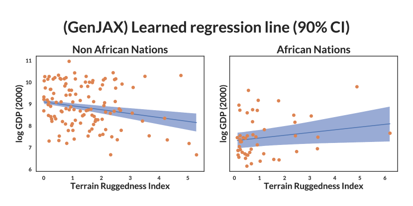
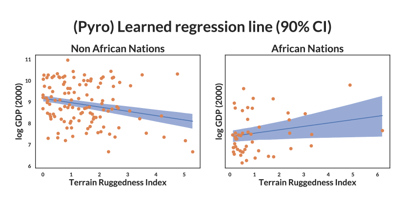
Figure 13. Final regression fits from variational inference. The variable cafrica denotes whether a country is in Africa. The variable ruggedness denotes the value of the country on the Terrain Ruggedness Index. Shaded blue is the 90% credible interval (CI) approximated by sampling (3200 samples).

D.3. Semi-supervised variational autoencoder

We consider the semi-supervised variational autoencoder (Kingma et al., 2014): a variational algorithm for settings where both unlabeled and labeled data are available. There are two models for this algorithm in $\lambda_{\text{Gen}}$, one for unsupervised training and one for supervised training:

$\textbf{unsup\_model}\coloneqq\lambda(img,\theta).(\textbf{do}\{$ $\quad\quad label\leftarrow\textbf{sample}~{}\textbf{categorical}(\textbf{map}~{}(\lambda v.\frac{v}{10})~{}(\textbf{ones}~{}10))~{}\text{"label"};$ $\quad\quad label_{\text{oh}}=\textbf{one\_hot}~{}label~{}10;$ $\quad\quad latent\leftarrow\textbf{sample}~{}\textbf{mv\_normal}((\textbf{zeros}~{}50),(\textbf{ones}~{}50))~{}\text{"latent"};$ $\quad\quad probs=\textbf{decoder}~{}\theta~{}latent~{}label_{\text{oh}};$ $\quad\quad\textbf{mapM}~{}(\lambda(p,px).~{}\textbf{observe}~{}(\textbf{bernoulli}(p)~{}px))~{}\mathbf{zip}(probs,img)$ $\})$

$\textbf{sup\_model}\coloneqq\lambda(label,img,\theta).(\textbf{do}\{$ $\quad\quad\textbf{observe}~{}\textbf{categorical}(\textbf{map}~{}(\lambda v.\frac{v}{10})~{}(\textbf{ones}~{}10))~{}label;$ $\quad\quad label_{\text{oh}}=\textbf{one\_hot}~{}label~{}10;$ $\quad\quad latent\leftarrow\textbf{sample}~{}\textbf{mv\_normal}((\textbf{zeros}~{}50),(\textbf{ones}~{}50))~{}\text{"latent"};$ $\quad\quad probs=\textbf{decoder}~{}\theta~{}latent~{}label_{\text{oh}};$ $\quad\quad\textbf{mapM}~{}(\lambda(p,px).~{}\textbf{observe}~{}(\textbf{bernoulli}(p)~{}px))~{}\mathbf{zip}(probs,img)$ $\})$

Figure 14. Models for semi-supervised learning. We make use of several helper functions: $\lambda v.\textbf{one\_hot}~{}v~{}N$ converts $\text{label}\in[0,N]\subset\mathbb{N}$ into a one-hot vector in $\mathbb{R}^{N}$. decoder represents a neural network: it accepts parameters $\theta$ and applies a network to the input latent and label_oh concatenated into a single vector.

Corresponding to each model, there is also a guide:

$\textbf{unsup\_guide}\coloneqq\lambda(img,\phi).(\textbf{do}\{$ $\quad\quad probs=\textbf{encoder}_{1}~{}(\pi_{1}~{}\phi)~{}img$ $\quad\quad label\leftarrow\textbf{sample}~{}\textbf{categorical}_{\text{ENUM}}(probs)~{}\text{"label"};$ $\quad\quad label_{\text{oh}}=\textbf{one\_hot}~{}label~{}10;$ $\quad\quad\phi_{\text{latent}}=\textbf{encoder}_{2}~{}(\pi_{2}~{}\phi)~{}label_{\text{oh}}~{}img;$ $\quad\quad latent\leftarrow\textbf{sample}~{}\textbf{mv\_normal}_{\text{REPARAM}}(\pi_{1}~{}\phi_{\text{latent}},\pi_{2}~{}\phi_{\text{latent}})~{}\text{"latent"};$ $\})$

$\textbf{sup\_guide}\coloneqq\lambda(label,img,\phi).(\textbf{do}\{$ $\quad\quad label_{\text{oh}}=\textbf{one\_hot}~{}label~{}10;$ $\quad\quad\phi_{\text{latent}}=\textbf{encoder}_{2}~{}(\pi_{2}~{}\phi)~{}label_{\text{oh}}~{}img;$ $\quad\quad latent\leftarrow\textbf{sample}~{}\textbf{mv\_normal}_{\text{REPARAM}}(\pi_{1}~{}\phi_{\text{latent}},\pi_{2}~{}\phi_{\text{latent}})~{}\text{"latent"};$ $\})$

Figure 15. Guides for semi-supervised learning.

The objective for supervised training is $\textbf{ELBO}(\textbf{sup\_model},\textbf{sup\_guide})$ and the objective for unsupervised training is $\textbf{ELBO}(\textbf{unsup\_model},\textbf{unsup\_guide})$. In the semi-supervised setting, the assumption is that a small amount of labeled data is available: the idea is that mixing unsupervised learning with supervised learning will allow the learning process to better use the labeled data.

In Fig. 16, we show the unsupervised loss (ELBO) curves for genjax.vi and Pyro. Both systems use the same hyperparameters, similar network architectures (genjax.vi uses SoftPlus activation instead of ReLU), and the same unsupervised / supervised training schedule (3000 supervised examples, with a round of supervised training every 16th batch). In Fig. 17, we show conditional generation from the learned SSVAE networks.

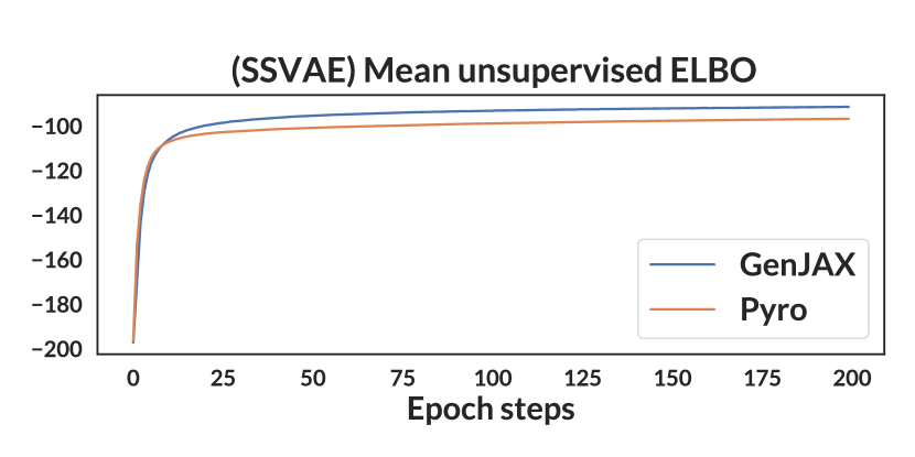
System	Average wall time per epoch	Average ELBO (last $100$ steps)
genjax.vi	0.41 (s)	-92.48
Pyro	3.98 (s)	-97.74

Figure 16. The mean (over batches) unsupervised loss (an ELBO objective) during training. genjax.vi and Pyro exhibit similar loss curves using the same gradient estimators for the ELBO.

genjax.vi

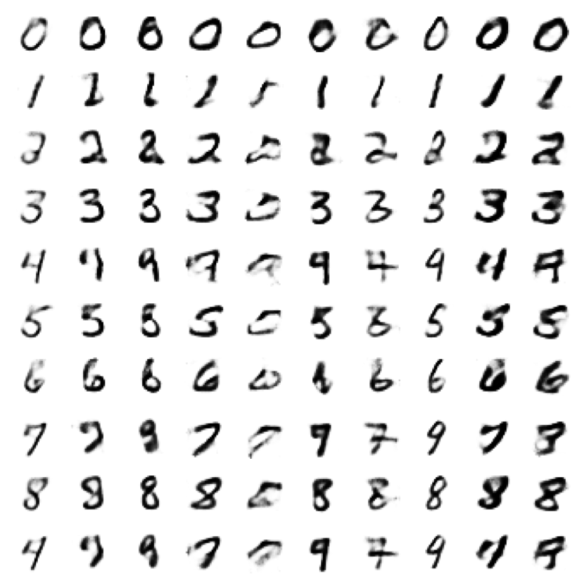
Pyro

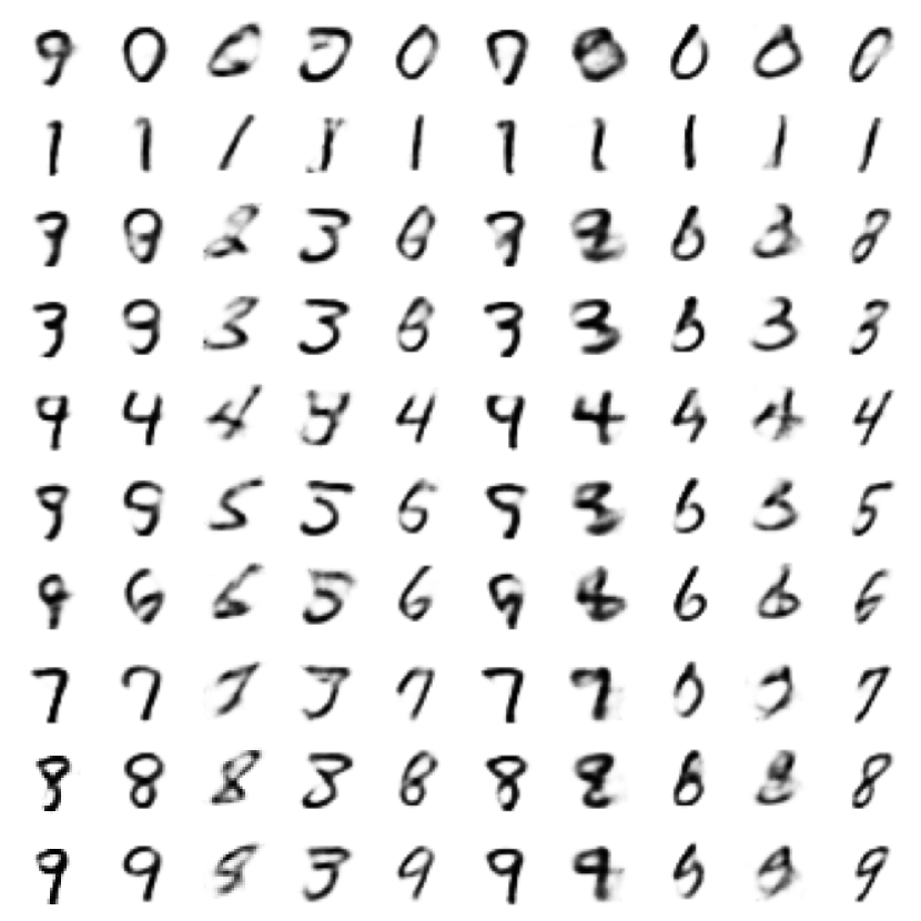
Figure 17. Conditional generation using trained SSVAE from (left) genjax.vi, and (right) Pyro. The resultant decoder models have similar visual fidelity. Samples were generated by fixing a random seed per column - each sampled image in a column has the same style (latent sample from multivariate Gaussian).

D.4. Conditional variational autoencoder

We consider the conditional variational autoencoder (Sohn et al., 2015). The learning task: given an observation of a quadrant of an MNIST image, fill in the other quadrants. The CVAE architecture consists of two components:

• A deterministic baseline network which looks at the observed quadrant and attempts to fill in the other quadrants. This network is trained using binary cross entropy loss applied pixel wise across the quadrants which are not conditioned on.

• A variational autoencoder, which is trained on the entire image. The architecture uses the trained baseline network as part of the model, to provide an initial guess for the rest of the image, which is then processed by the decoder networks.

genjax.vi

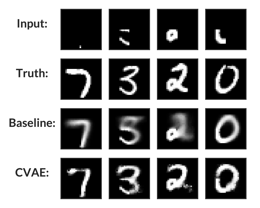
NumPyro

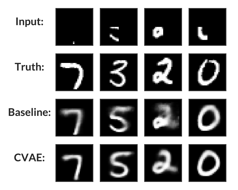
Figure 18. Conditional generation using the CVAE networks learned by genjax.vi and NumPyro. The input is the lower left quadrant of an MNIST digit image: the CVAE attempts to fill in the other quadrants. Both genjax.vi and NumPyro learn approximations with similar reconstruction accuracy.

System	Average wall time per epoch
genjax.vi	0.36 (s)
Pyro	5.73 (s)
NumPyro	1.36 (s)

Figure 19. Wall clock time comparisons for the conditional VAE.

Appendix E Proof Details

This section provides details on the proofs of several results stated in the main paper.

E.1. Definition of helper functions pop and split

Our semantics is defined in part using helper functions, pop and $\textit{split}_{\mu}$, that we define here.

Definition of pop. For each base type $\sigma$, we define $\textit{pop}_{\sigma}:\mathbb{T}\times\text{Str}\to\sigma\times\mathbb{R}\times\mathbb{T}$ to return, on input $(u,k)$, the tuple $(x,1,u^{\prime})$ when $u=u^{\prime}\mathbin{+\mkern-5.0mu+}\{k\mapsto x\}$ for some $x\in\llbracket\sigma\rrbracket$, and the tuple $(\text{default}_{\sigma},0,\{\})$ when $u$ does not map the key $k$ to a value of type $\sigma$. When clear from context, we omit the type $\sigma$.

Definition of split. Suppose $\mu$ is a discrete-structured measure on $\mathbb{T}$, absolutely continuous with respect to $\mathcal{B}_{\mathbb{T}}$. Define $\mathbb{T}_{\mu}\subseteq\mathbb{T}$ to be the support of $\mu$. For a given trace $u\in\mathbb{T}$, define $\text{subtraces}(u):=\{u^{\prime}\in\mathbb{T}\mid\exists u^{\prime\prime}\in\mathbb{T}.u^{\prime}\mathbin{+\mkern-5.0mu+}u^{\prime\prime}=u\}$ to be the set of $u$’s subtraces. Note that for all $u\in\mathbb{T}$, the intersection $\mathbb{T}_{\mu}\cap\text{subtraces}(u)$ is either empty, or a singleton set $\{u^{*}\}$. This is because, if there were two distinct traces $u_{1}^{*}$ and $u_{2}^{*}$ in the intersection, then by the discrete-structured condition, they would need to disagree on the value of some choice $k$ present in both $u_{1}^{*}$ and $u_{2}^{*}$. But this is not possible, since both traces are subtraces of $u$, and so agree with $u$ (and therefore with each other) for every choice $k$ that they share in common.

The function $\textit{split}_{\mu}(u)$ is defined to equal $(u,\{\})$ when $\mathbb{T}_{\mu}\cap\text{subtraces}(u)$ is empty, and $(u^{*},u-u^{*})$ when $\mathbb{T}_{\mu}\cap\text{subtraces}(u)$ is non-empty. (Here, $u-u^{*}$ is the subtrace of $u$ that has only keys $k$ which do not appear in $u^{*}$.)

E.2. Well-definedness of the semantics

Our semantics of $\lambda_{\text{Gen}}$ (Fig. 4) interprets programs of type $G~{}\tau$ as elements of $\text{Meas}_{\ll\mathcal{B}_{\mathbb{T}}}^{DS}~{}\mathbb{T}$, a subspace of particularly well-behaved measures on $\mathbb{T}$. We must therefore prove that our term semantics actually does assign to every term of type $G~{}\tau$ a well-behaved measure over traces.

Lemma E.1.

Let $\Gamma\vdash t:\tau$ be a $\lambda_{\text{Gen}}$ term, and let $\gamma\in\llbracket\Gamma\rrbracket$. Then $\llbracket t\rrbracket(\gamma)$, as defined inductively in Figure 4, lies in $\llbracket\tau\rrbracket$. In particular, if $\tau=G~{}\tau^{\prime}$ for some type $\tau^{\prime}$, then $\llbracket t\rrbracket_{1}(\gamma)$ is discrete-structured and absolutely continuous with respect to $\mathcal{B}_{\mathbb{T}}$.

Proof.

The proof is by induction on the derivation of $\Gamma\vdash t:\tau$. The only non-trivial cases are when $t$ builds a new probabilistic program of type $\tau=G~{}\tau^{\prime}$, and the only non-trivial conditions to prove are discrete structure and absolute continuity of trace distribution.

We consider these non-trivial cases in turn:

• $t=\mathbf{return}~{}t^{\prime}$: in this case, $\llbracket t\rrbracket_{1}(\gamma)$ is the Dirac measure on the empty trace, $\delta_{\{\}}$. This measure is clearly absolutely continuous with respect to $\mathcal{B}_{\mathbb{T}}$ (it has density $1$ at the point $\{\}$, and $0$ elsewhere), and is also clearly discrete-structured (vacuously, as there are no two distinct traces to which it assigns positive density).

• $t=\textbf{observe}~{}t_{1}~{}t_{2}$: in this case, $\llbracket t\rrbracket_{1}(\gamma)$ is a rescaled Dirac measure, $w\odot\delta_{\{\}}$. By the same argument as above, it is absolutely continuous with respect to $\mathcal{B}_{\mathbb{T}}$ (its density is $w$ at $\{\}$ and $0$ elsewhere), and discrete-structured (again, there are no two distinct traces to which it assigns positive density).

• $t=\textbf{sample}~{}t_{1}~{}t_{2}$: in this case, $\llbracket t\rrbracket_{1}(\gamma)$ is the pushforward of a measure $\mu=\llbracket t_{1}\rrbracket(\gamma)$ on $\tau^{\prime}$ by the map $\lambda x.\{\llbracket t_{2}\rrbracket(\gamma)\mapsto x\}$. Because $\mu$ is (by the inductive hypothesis) absolutely continuous with respect to the base measure on $\tau^{\prime}$, our new measure $\llbracket t\rrbracket_{1}(\gamma)$ is absolutely continuous with respect to $\mathcal{B}_{\mathbb{T}}$, with density $\frac{d\mu}{d\mathcal{B}_{\tau^{\prime}}}(x)$ for traces of the form $\{\llbracket t_{2}\rrbracket(\gamma)\mapsto x\}$, and density 0 for all other traces. It is also discrete-structured, because any two traces with positive density must have the form $\{\llbracket t_{2}\rrbracket(\gamma)\mapsto x\}$ for distinct values of $x$—so $\llbracket t_{2}\rrbracket(\gamma)$ is an address on which they are guaranteed to disagree.

• $t=\textbf{do}\{x\leftarrow t_{1};m\}$: by induction, $\llbracket t_{1}\rrbracket_{1}(\gamma)$ is absolutely continuous with respect to $\mathcal{B}_{\mathbb{T}}$, and so is $\llbracket\textbf{do}\{m\}\rrbracket_{1}(\gamma[x\mapsto v])$, for all $v\in\llbracket\tau_{1}\rrbracket$ (where $G~{}\tau_{1}$ is the type of $t_{1}$). Thus, the joint distribution is also absolutely continuous with respect to $\mathcal{B}_{\mathbb{T}}$, with density equal to the product of the component densities. For discrete structure, let $u$ and $u^{\prime}$ be distinct traces in the support of $\llbracket t\rrbracket_{1}(\gamma)$. Let $(u_{1},u_{2})=\text{split}_{\llbracket t_{1}\rrbracket_{1}(\gamma)}(u)$, and likewise let $(u_{1}^{\prime},u_{2}^{\prime})=\text{split}_{\llbracket t_{1}\rrbracket_{1}(\gamma)}(u^{\prime})$. If $u_{1}\neq u_{1}^{\prime}$, then since they are both in the support of $\llbracket t_{1}\rrbracket_{1}(\gamma)$, by induction they must share an address to which they assign different values, an address on which $u$ and $u^{\prime}$ would therefore also disagree. If $u_{1}=u_{1}^{\prime}$ and $u_{2}\neq u_{2}^{\prime}$, then since both $u_{2}$ and $u_{2}^{\prime}$ are in the support of $\llbracket\textbf{do}\{m\}\rrbracket(\gamma[x\mapsto\llbracket t_{1}\rrbracket_{2}(\gamma)(u_{1})])$ (which is discrete-structured by induction), there must be a shared address on which they disagree. This would again constitute a shared address on which $u$ and $u^{\prime}$ disagree.

∎

E.3. Proof details for Lemma 4.1

Proof.

Lemma 4.1 is an instance of the fundamental lemma of logical relations, for the particular logical relations $\mathcal{R}^{\xi}$.

We consider a term $\Gamma\vdash t:\tau^{*}$ and an arbitrary pair of environments $(\gamma,\gamma^{\prime})\in\mathcal{R}_{\Gamma}^{\xi}$. Note that when $t=x$, $t=(t_{1},t_{2})$, $t=\pi_{i}~{}t^{\prime}$, $t=\lambda x.t^{\prime}$, $t=t_{1}~{}t_{2}$, or $t=\mathbf{if}~{}t_{1}~{}\mathbf{then}~{}t_{1}~{}\mathbf{else}~{}t_{2}$, we can apply the standard logical relations arguments, because our semantics and logical relations for product types, function types, Booleans, and variables are completely standard, and the macro $\xi$ treats these constructs functorially (e.g. $\xi\{(t_{1},t_{2})\}=(\xi\{t_{1}\},\xi\{t_{2}\})$). We establish the remaining cases in turn.

• If $\tau^{*}$ is some base type $\sigma$ and $t=c$ (a constant of type $\sigma$), then $\xi\{t\}=t$ and it follows immediately that $(\llbracket t\rrbracket(\gamma),\llbracket\xi\{t\}\rrbracket(\gamma^{\prime}))\in\mathcal{R}_{\sigma}^{\xi}$ (which is just the equality relation).

• If $t=\mathbf{normal}_{\text{REPARAM}}$, $t=\mathbf{normal}_{\text{REINFORCE}}$, or $t=\mathbf{flip}_{\text{MVD}}$, then no matter what $\gamma$ and $\gamma^{\prime}$ are, $\llbracket t\rrbracket(\gamma)$ is a primitive probability kernel (e.g., the normal distribution or the Bernoulli distribution), and $\llbracket\xi\{t\}\rrbracket(\gamma^{\prime})$ is a primitive density function. We discharge this case by verifying that the primitive density functions are correctly implemented.

• The key cases of interest are the terms of type $\tau^{*}=G~{}\tau$. For each, we need to establish several key properties of $\xi\{t\}$, outlined in the definition of $\mathcal{R}_{G~{}\tau}^{\xi}$. In each of the cases below, let $(\mu,f)=\llbracket t\rrbracket(\gamma)$, let $u$ be a trace, and let $(u_{1},u_{2})=\textit{split}_{\mu}(u)$. Further, let $g=\llbracket\xi\{t\}\rrbracket(\gamma^{\prime})$. We write $g_{i}$ (for $i$ in $\{1,2,3\}$) as shorthand for $\pi_{i}\circ g$. Our job is to show that in each case below, $(f(u),g_{1}(u))\in R_{\tau}^{\xi}$, that $g_{2}(u)=\frac{d\mu}{d\mathcal{B}_{\mathbb{T}}}(u_{1})$, and that $g_{3}(u)=u_{2}$.

  • $t=\mathbf{return}~{}t^{\prime}$: From the semantics of $\lambda_{\text{Gen}}$, we have $\mu=\delta_{\{\}}$ and $f=\lambda\_.\llbracket t^{\prime}\rrbracket(\gamma)$. Then for any $u$, we have that $(u_{1},u_{2})=(\{\},u)$. We now establish each requirement:

    1. From the definition of $\xi\{\mathbf{return}~{}t^{\prime}\}$, we have $g_{1}(u)=\llbracket\xi\{t^{\prime}\}\rrbracket(\gamma^{\prime})$, so by the inductive hypothesis for $\Gamma\vdash t^{\prime}:\tau^{\prime}$, $(f(u),g_{1}(u))\in R_{\tau}^{\xi}$.

    2. Also from the definition of $\xi\{\mathbf{return}~{}t^{\prime}\}$, we have $g_{2}(u)=1$ for all $u$, which, as required, is equal to $\frac{d\mu}{d\mathcal{B}_{\mathbb{T}}}(u_{1})$ (since $u_{1}=\{\}$ and $\mu=\delta_{\{\}}$).

    3. Finally, we can read off the definition of $\xi\{\mathbf{return}~{}t^{\prime}\}$ that $g_{3}(u)=u$ for all $u$, which is equal to $u_{2}$, as required.

  • $t=\mathbf{observe}~{}t_{1}~{}t_{2}$: Write $\sigma$ for the type of $t_{2}$, and let $m=\llbracket t_{1}\rrbracket(\gamma)$ and $v=\llbracket t_{2}\rrbracket(\gamma)$. By induction, $\llbracket\xi\{t_{1}\}\}\rrbracket(\gamma^{\prime})=\frac{dm}{d\mathcal{B}_{\sigma}}$, and $\llbracket\xi\{t_{2}\}\rrbracket(\gamma^{\prime})=v$. From the semantics, we see that $\mu=\frac{dm}{d\mathcal{B}_{\sigma}}(v)\odot\delta_{\{\}}$, and that $f=\lambda\_.()$. As in the previous case, $(u_{1},u_{2})=(\{\},u)$.

    1. We have $g_{1}(u)=()$, and so $(f(u),g_{1}(u))=((),())\in R_{1}^{\xi}$.

    2. We have $g_{2}(u)=\llbracket\xi\{t_{1}\}\rrbracket(\gamma^{\prime})(\llbracket\xi\{t_{2}\}\rrbracket(\gamma^{\prime}))=\frac{dm}{d\mathcal{B}_{\sigma}}(v)$. But this is precisely the density of $\mu$ with respect to $\mathcal{B}_{\mathbb{T}}$ at the point $u_{1}=\{\}$, because $\mu=\frac{dm}{d\mathcal{B}_{\sigma}}(v)\odot\delta_{\{\}}$.

    3. Finally, we have $g_{3}(u)=u$, which is equal to $u_{2}$, as required.

  • $t=\mathbf{sample}~{}t_{1}~{}t_{2}$: In this case $\tau$ is some base type $\sigma$. Let $m=\llbracket t_{1}\rrbracket(\gamma)$ and $k=\llbracket t_{2}\rrbracket(\gamma)$, and note that by induction, $\llbracket\xi\{t_{1}\}\rrbracket(\gamma^{\prime})=\frac{dm}{d\mathcal{B}_{\sigma}}$ and $\llbracket\xi\{t_{2}\}\rrbracket(\gamma^{\prime})=k$. From the semantics, we have that $\mu$ is the pushforward of $m$ by $v\mapsto\{k\mapsto v\}$. We consider two cases. First, suppose the trace $u$ does not have key $k$. Then $f(u)$ is equal to a default value of type $\sigma$, and $(u_{1},u_{2})=(u,\{\})$. In this case, $\textit{pop}~{}u~{}k$ returns the default value of type $\sigma$, the weight $0$, and the remainder $\{\}$, and we reason as follows:

    1. $g_{1}(u)$ is the default value of type $\sigma$, which is equal to $f(u)$, so $(f(u),g_{1}(u))\in R_{\sigma}^{\xi}$.

    2. $g_{2}(u)$ is 0, which is the density under $\mu$ of $u_{1}=u$, because $u_{1}$ does not have key $k$, but $\mu$ assigns positive density only to traces that do have key $k$.

    3. $g_{3}(u)=\{\}=u_{2}$, as required.

    Alternatively, suppose the trace $u$ does have key $k$, assigned to value $v$. In this case, $f(u)=v$, and $(u_{1},u_{2})=(\{k\mapsto v\},u-\{k\mapsto v\})$, and the result of $\textit{pop}~{}u~{}k$ is $(v,1,u_{2})$. In this case:

    1. $g_{1}(u)=v=f(u)$, and so $(f(u),g_{1}(u))\in R_{\sigma}^{\xi}$.

    2. $g_{2}(u)=\llbracket\xi\{t_{1}\}\rrbracket(\gamma^{\prime})(v)=\frac{dm}{d\mathcal{B}_{\sigma}}(v)=\frac{d\mu}{d\mathcal{B}_{\mathbb{T}}}(\{k\mapsto v\})=\frac{d\mu}{d\mathcal{B}_{\mathbb{T}}}(u_{1})$, as required.

    3. $g_{3}(u)=u-\{k\mapsto v\}=u_{2}$, as required.

  • $t=\textbf{do}\{x\leftarrow t^{\prime};m\}$: Let $\tau^{\prime}$ be the type of the intermediate result, i.e., the type such that $t^{\prime}$ has type $G~{}\tau^{\prime}$. Let $(\mu^{\prime},f^{\prime})=\llbracket t^{\prime}\rrbracket(\gamma)$, let $k=\lambda x.\llbracket\textbf{do}\{m\}\rrbracket_{1}(\gamma)$, and let $f_{k}(v)=\llbracket\textbf{do}\{m\}\rrbracket_{2}(\gamma[x\mapsto v])$. Then $\mu(U)=\iint\textit{disj}(r_{1},r_{2})\cdot\delta_{r_{1}\mathbin{+\mkern-5.0mu+}r_{2}}(U)\mu^{\prime}(dr_{1})k(f^{\prime}(r_{1}),dr_{2})$.

    We now consider several possible scenarios.

    • First, suppose no subtrace of $u$ is in the support of $\mu^{\prime}$, so that $(u_{1},u_{2})=(u,\{\})$. Then by induction, $\llbracket\xi\{t^{\prime}\}\rrbracket(\gamma^{\prime})(u)$ returns $(v,0,\{\})$ for some value $v$ such that $(f^{\prime}(u),v)\in R_{\tau^{\prime}}^{\xi}$. Because $(f^{\prime}(u),v)\in R_{\tau^{\prime}}^{\xi}$, we have that $(\gamma[x\mapsto f^{\prime}(u)],\gamma^{\prime}[x\mapsto v])\in R_{\Gamma,x:\tau^{\prime}}^{\xi}$. We can then apply the inductive hypothesis for $\Gamma,x:\tau^{\prime}\vdash\textbf{do}\{m\}:G~{}\tau$, with these two environments, to obtain that $\llbracket\xi\{\textbf{do}\{m\}\}\rrbracket(\gamma^{\prime}[x\mapsto v])(\{\})=(y,w,\{\})$, for some weight $w$ and some value $y$ such that $(f_{k}(f^{\prime}(u))(\{\}),y)\in R_{\tau}^{\xi}$. We can then read off the definition of $\xi\{\textbf{do}\{x\leftarrow t^{\prime};m\}\}$ that $g_{1}(u)=y$, $g_{2}(u)=0\cdot w=0$, and $g_{3}(u)=\{\}$. Now consider each requirement:

      1. From the semantics of do, we have that $f(u)=f_{k}(f^{\prime}(u))(\{\})$. We also have from above that $g_{1}(u)=y$, which is related at $R_{\tau}^{\xi}$ to $f_{k}(f^{\prime}(u))(\{\})$, as required.

      2. We have $g_{2}(u)=0$, which is (as required) the density of $\mu$ at $u$ (since $u$ is not in $\mu$’s support).

      3. We have $g_{3}(u)=\{\}=u_{2}$, as required.

    • Second, suppose there is a subtrace in the support of $\mu^{\prime}$, but that, writing $(u^{\prime}_{1},u^{\prime}_{2})=\textit{split}_{\mu^{\prime}}(u)$, there is no subtrace of $u^{\prime}_{2}$ in the support of $k(f^{\prime}(u))$. Then $(u_{1},u_{2})=(u,\{\})$ once again. By induction, $\llbracket\xi\{t^{\prime}\}\rrbracket(\gamma^{\prime})(u)=(v,w,u^{\prime}_{2})$, for some $v$ such that $(f^{\prime}(u),v)\in R_{\tau^{\prime}}^{\xi}$ and some $w>0$. Now, since no subtrace of $u^{\prime}_{2}$ is in the support of $k(f^{\prime}(u))$, $\textit{split}_{k(f(u))}(u^{\prime}_{2})=(u^{\prime}_{2},\{\})$. Also, since $(f^{\prime}(u),v)\in R_{\tau^{\prime}}^{\xi}$, we can construct extended environments $(\gamma[x\mapsto f^{\prime}(u)],\gamma^{\prime}[x\mapsto v])\in R_{\Gamma,x:\tau^{\prime}}^{\xi}$. Then, by the inductive hypothesis for $\Gamma,x:\tau^{\prime}\vdash\textbf{do}\{m\}:G~{}\tau$, we have that $\llbracket\xi\{\textbf{do}\{m\}\}\rrbracket(\gamma^{\prime}[x\mapsto v])(u^{\prime}_{2})=(y,0,\{\})$ such that $(f_{k}(f^{\prime}(u))(u^{\prime}_{2}),y)\in R_{\tau}^{\xi}$. Then $g_{1}(u)=y$, $g_{2}(u)=w\cdot 0=0$, and $g_{3}(u)=\{\}$. We can again consider each requirement, using the same arguments as in the first case:

      1. From the semantics of do, we have that $f(u)=f_{k}(f^{\prime}(u))(u^{\prime}_{2})$. We also have from above that $g_{1}(u)=y$, which is related at $R_{\tau}^{\xi}$ to $f_{k}(f^{\prime}(u))(\{\})$, as required.

      2. We have $g_{2}(u)=0$, which is (as required) the density of $\mu$ at $u$ (since $u$ is not in $\mu$’s support).

      3. We have $g_{3}(u)=\{\}=u_{2}$, as required.

    • Finally, suppose that $u$ has a subtrace in the support of $\mu$ (in which case that subtrace must be the one computed by $\textit{split}_{\mu}$, namely $u_{1}$). For this to be the case, $u_{1}$ must decompose as $u^{\prime}_{1}\mathbin{+\mkern-5.0mu+}u^{\prime}_{2}$, where $(u^{\prime}_{1},u^{\prime}_{2})=\textit{split}_{\mu^{\prime}}(u_{1})$. Furthermore, we have that $\textit{split}_{\mu^{\prime}}(u)=(u^{\prime}_{1},u^{\prime}_{2}\mathbin{+\mkern-5.0mu+}u_{2})$. By induction on $\Gamma\vdash t^{\prime}:G~{}\tau^{\prime}$, we have that $\llbracket\xi\{t^{\prime}\}\rrbracket(\gamma^{\prime})(u)=(v,\frac{d\mu^{\prime}}{d\mathcal{B}_{\mathbb{T}}}(u^{\prime}_{1}),u^{\prime}_{2}\mathbin{+\mkern-5.0mu+}u_{2})$ for some $v$ satisfying $(f^{\prime}(u),v)\in R_{\tau^{\prime}}^{\xi}$. We can construct extended environments $(\gamma[x\mapsto f^{\prime}(u)],\gamma^{\prime}[x\mapsto v])\in R_{\Gamma,x:\tau^{\prime}}^{\xi}$, and apply the inductive hypothesis for $\Gamma,x:\tau^{\prime}\vdash\textbf{do}\{m\}:G~{}\tau$, to obtain that $\llbracket\xi\{\textbf{do}\{m\}\}\rrbracket(\gamma^{\prime}[x\mapsto v])(u^{\prime}_{2}\mathbin{+\mkern-5.0mu+}u_{2})=(y,\frac{dk(f^{\prime}(u))}{d\mathcal{B}_{\mathbb{T}}}(u^{\prime}_{2}),u_{2})$ for some $y$ such that $(f_{k}(f^{\prime}(u))(u^{\prime}_{2}\mathbin{+\mkern-5.0mu+}u_{2}),y)\in R_{\tau}^{\xi}$. Then $g_{1}(u)=y$, $g_{2}(u)=\frac{d\mu^{\prime}}{d\mathcal{B}_{\mathbb{T}}}(u^{\prime}_{1})\cdot\frac{dk(f^{\prime}(u))}{d\mathcal{B}_{\mathbb{T}}}(u^{\prime}_{2})$, and $g_{3}(u)=u_{2}$. We now verify the requirements:

      1. From the semantics of do, we have that $f(u)=f_{k}(f^{\prime}(u))(u^{\prime}_{2}\mathbin{+\mkern-5.0mu+}u_{2})$. We also have from above that $g_{1}(u)=y$, which is related at $R_{\tau}^{\xi}$ to $f_{k}(f^{\prime}(u))(u^{\prime}_{2}\mathbin{+\mkern-5.0mu+}u_{2})$, as required.

      2. We have $g_{2}(u)=\frac{d\mu^{\prime}}{d\mathcal{B}_{\mathbb{T}}}(u^{\prime}_{1})\cdot\frac{dk(f^{\prime}(u))}{d\mathcal{B}_{\mathbb{T}}}(u^{\prime}_{2})=\frac{d\mu}{d\mathcal{B}_{\mathbb{T}}}(u^{\prime}_{1}\mathbin{+\mkern-5.0mu+}u^{\prime}_{2})$, which is (as required) the density of $\mu$ at $u_{1}=u^{\prime}_{1}\mathbin{+\mkern-5.0mu+}u^{\prime}_{2}$.

      3. We have $g_{3}(u)=u_{2}$, as required.

∎

E.4. Proof details for Lemma 4.3

Proof.

Lemma 4.3 is an instance of the fundamental lemma of logical relations, for the particular logical relations $\mathcal{R}^{\chi}$.

We consider a term $\Gamma\vdash t:\tau^{*}$ and an arbitrary pair of environments $(\gamma,\gamma^{\prime})\in\mathcal{R}_{\Gamma}^{\chi}$. Note that when $t=x$, $t=(t_{1},t_{2})$, $t=\pi_{i}~{}t^{\prime}$, $t=\lambda x.t^{\prime}$, $t=t_{1}~{}t_{2}$, or $t=\mathbf{if}~{}t_{1}~{}\mathbf{then}~{}t_{1}~{}\mathbf{else}~{}t_{2}$, we can again apply the standard logical relations arguments, because our semantics and logical relations for product types, function types, Booleans, and variables are completely standard, and the macro $\chi$ treats these constructs functorially (e.g. $\chi\{(t_{1},t_{2})\}=(\chi\{t_{1}\},\chi\{t_{2}\})$). We establish the remaining cases in turn.

• If $\tau^{*}$ is some base type $\sigma$ and $t=c$ (a constant of type $\sigma$), then $\xi\{t\}=t$ and it follows immediately that $(\llbracket t\rrbracket(\gamma),\llbracket\chi\{t\}\rrbracket(\gamma^{\prime}))\in\mathcal{R}_{\sigma}^{\chi}$ (which is just the equality relation).

• If $t=\mathbf{normal}_{\text{REPARAM}}$, $t=\mathbf{normal}_{\text{REINFORCE}}$, or $t=\mathbf{flip}_{\text{MVD}}$, then no matter what $\gamma$ and $\gamma^{\prime}$ are, $\llbracket t\rrbracket(\gamma)$ is a primitive probability kernel (e.g., the normal distribution or the Bernoulli distribution), and $\llbracket\chi\{t\}\rrbracket(\gamma^{\prime})$ has two components: a primitive simulator for the distribution, simulating an outcome and evaluating its density, and a deterministic density function. We discharge this case by verifying that the primitive simulators generate from the correct primitive distributions and evaluate the corresponding primitive densities.

• The key cases of interest are the terms of type $\tau^{*}=G~{}\tau$. For each, we need to establish several key properties of $\chi\{t\}$, outlined in the definition of $\mathcal{R}_{G~{}\tau}^{\chi}$. In each of the cases below, let $(\mu,f)=\llbracket t\rrbracket(\gamma)$, let $\nu=\llbracket\chi\{t\}\rrbracket(\gamma^{\prime})$, and let $u$ be a trace in the support of $\mu$. In each case below, we first establish that $\nu$ is the pushforward of $\mu$ by a map $h$; writing $h_{i}$ for $\pi_{i}\circ h$, we then show that $(f(u),h_{1}(u))\in R_{\tau}^{\chi}$, $h_{2}(u)=\frac{d\mu}{d\mathcal{B}_{\mathbb{T}}}(u)$, and $h_{3}(u)=u$.

  • $t=\mathbf{return}~{}t^{\prime}$: We have $\mu=\delta_{\{\}}$ and $f=\lambda\_.\llbracket t^{\prime}\rrbracket(\gamma)$. Examining the rule for $\chi$ on this expression, we see that $\nu$ is a pushforward of $\mu$ by $h(u)=(\llbracket\chi\{t^{\prime}\}\rrbracket(\gamma^{\prime}),1,\{\})$. Note also that the only trace in the support of $\mu$ is $\{\}$, so $u$ must be $\{\}$. We establish the three required properties:

    1. We have $h_{1}(u)=\llbracket\chi\{t^{\prime}\}\rrbracket(\gamma^{\prime})$, which is related to $f(u)=\llbracket t^{\prime}\rrbracket(\gamma)$ by the inductive hypothesis for $\Gamma\vdash t:\tau$.

    2. We have $h_{2}(u)=1=\frac{d\mu}{d\mathcal{B}_{\mathbb{T}}}(u)$ (since $u=\{\}$), as required.

    3. We have $h_{3}(u)=\{\}=u$, as required.

  • $t=\mathbf{observe}~{}t_{1}~{}t_{2}$: Write $\sigma$ for the type of $t_{2}$, and let $m=\llbracket t_{1}\rrbracket(\gamma)$ and $v=\llbracket t_{2}\rrbracket(\gamma)$. By induction, $\pi_{2}(\llbracket\chi\{t_{1}\}\}\rrbracket(\gamma^{\prime}))$ is $\frac{dm}{d\mathcal{B}_{\sigma}}$, and $\llbracket\chi\{t_{2}\}\rrbracket(\gamma^{\prime})=v$. From the semantics, we see that $\mu=\frac{dm}{d\mathcal{B}_{\sigma}}(v)\odot\delta_{\{\}}$, and that $f=\lambda\_.()$. From the definition of $\chi$, we see that the generated code first computes the deterministic constant $w=\pi_{1}(\llbracket\chi\{t_{1}\}\rrbracket(\gamma^{\prime}))(\llbracket\chi\{t_{2}\}\rrbracket(\gamma^{\prime}))=\frac{dm}{d\mathcal{B}_{\sigma}}(v)$. Then we can see that the code implements the pushforward of $\mu=w\odot\delta_{\{\}}$ by $h(u)=((),w,\{\})$. Again, we know that $u$ must be $\{\}$, the only trace in the support of $\mu$. We then verify:

    1. We have $h_{1}(u)=()$, which is related to $f(u)=()$ in $R_{1}^{\chi}$.

    2. We have $h_{2}(u)=w=\frac{d\mu}{d\mathcal{B}_{\mathbb{T}}}(u)$ (since $u=\{\}$), as required.

    3. We have $h_{3}(u)=\{\}=u$, as required.

  • $t=\mathbf{sample}~{}t_{1}~{}t_{2}$: Let $m=\llbracket t_{1}\rrbracket(\gamma)$ and $k=\llbracket t_{2}\rrbracket(\gamma)=\llbracket\chi\{t_{2}\}\rrbracket(\gamma^{\prime})$ (where the last equality holds by the inductive hypothesis for $\Gamma\vdash t_{2}:\text{Str}$). We have that $\mu$ is the pushforward of $m$ by the map $\lambda x.\{k\mapsto x\}$, and that $f(u)=x$ when $u$ is of the form $\{k\mapsto x\}$. We also have, by the inductive hypothesis for $\Gamma\vdash t_{1}:D~{}\tau$, that $\pi_{1}(\llbracket\chi\{t_{1}\}\rrbracket(\gamma^{\prime}))$ is the pushforward of $m$ by $\lambda x.(x,\frac{dm}{d\mathcal{B}_{\tau}}(x))$. Then, from the definition of $\chi$, we have that $\llbracket\chi\{t\}\rrbracket(\gamma^{\prime})$ is the pushforward of $m$ by $\lambda x.(x,\frac{dm}{d\mathcal{B}_{\tau}}(x),\{k\mapsto x\})$, which is equivalently the pushforward of $\mu$ by $h=\lambda u.(f(u),\frac{dm}{d\mathcal{B}_{\tau}}(f(u)),u)$. Since $u$ is in the support of $\mu$, $u$ must have the form $\{k\mapsto x\}$ for some $x$. We verify:

    1. We have $h_{1}(u)=f(u)=x$, and $(f(u),x)=(x,x)\in R_{\tau}^{\chi}$, because $\tau$ is a base type so $R_{\tau}^{\chi}$ is the equality relation.

    2. We have $h_{2}(u)=\frac{dm}{d\mathcal{B}_{\tau}}(x)=\frac{d\mu}{d\mathcal{B}_{\mathbb{T}}}(\{k\mapsto x\})$, as required.

    3. We have $h_{3}(u)=u$, as required.

  • $t=\textbf{do}\{x\leftarrow t^{\prime};m\}$: Let $(\mu^{\prime},f^{\prime})=\llbracket t^{\prime}\rrbracket(\gamma)$, $k=\lambda v.\pi_{1}(\llbracket\textbf{do}\{m\}\rrbracket(\gamma[x\mapsto v]))$, and $f_{k}=\lambda v.\pi_{2}(\llbracket\textbf{do}\{m\}\rrbracket(\gamma[x\mapsto v]))$. By the inductive hypotheses for $\Gamma\vdash t^{\prime}:G~{}\tau^{\prime}$, we have that $\llbracket\chi\{t^{\prime}\}\rrbracket(\gamma^{\prime})$ is the pushforward of $\mu^{\prime}$ by a map $h^{\prime}(u^{\prime})$, such that $(f^{\prime}(u^{\prime}),h^{\prime}_{1}(u^{\prime}))\in R_{\tau^{\prime}}^{\chi}$, $h^{\prime}_{2}(u^{\prime})=\frac{d\mu^{\prime}}{d\mathcal{B}_{\mathbb{T}}}(u^{\prime})$, and $h^{\prime}_{3}(u^{\prime})=u^{\prime}$. Furthermore, we have that for any $u^{\prime}$ in the support of $\mu^{\prime}$, $\llbracket\chi\{\textbf{do}\{m\}\}\rrbracket(\gamma^{\prime}[x\mapsto h_{1}(u^{\prime})])$ is the pushforward of $k(f^{\prime}(u^{\prime}))$ by a function $h^{u^{\prime}}$, such that for all $u_{k}$ in the support of $k(f^{\prime}(u^{\prime}))$, $(f_{k}(f^{\prime}(u^{\prime}))(u_{k}),h^{u^{\prime}}_{1}(u_{k}))\in R_{\tau}^{\chi}$, $h^{u^{\prime}}_{2}(u_{k})=\frac{dk(f^{\prime}(u^{\prime}))}{d\mathcal{B}_{\mathbb{T}}}(u_{k})$, and $h_{3}^{u^{\prime}}(u_{k})=u_{k}$. Examining $\chi$’s definition for do, we see that $\nu$ is the pushforward of $\mu$ by $h(u)=(h_{1}^{u^{\prime}}(u_{k}),h_{2}^{u^{\prime}}(u_{k}),h_{3}^{u^{\prime}}(u_{k}))$, where $(u^{\prime},u_{k})=\textit{split}_{\mu^{\prime}}(u)$. We verify:

    1. We have $h_{1}(u)=h_{1}^{u^{\prime}}(u_{k})$, which we saw above is related by $R_{\tau}^{\chi}$ to $f(u)=f_{k}(f^{\prime}(u^{\prime}))(u_{k})$.

    2. We have $h_{2}(u)=h_{2}^{u^{\prime}}(u_{k})$, which, from above, is equal to $\frac{d\mu^{\prime}}{d\mathcal{B}_{\mathbb{T}}}(u^{\prime})\cdot\frac{dk(f^{\prime}(u^{\prime}))}{d\mathcal{B}_{\mathbb{T}}}(u_{k})$. This in turn is equal to $\frac{d\mu}{d\mathcal{B}_{\mathbb{T}}}(u)$, for $u$ in the support of $\mu$.

    3. We have $h_{3}(u)=h^{\prime}_{3}(u^{\prime})\mathbin{+\mkern-5.0mu+}h^{u^{\prime}}_{3}(u_{k})=u^{\prime}\mathbin{+\mkern-5.0mu+}u_{k}=u$, as required.

∎

Appendix F Adding New Primitives with Custom Gradient Estimators

In this appendix, we explain the process of extending our system with a new stochastic primitive, with its own custom gradient estimation strategy. In particular, we discuss the local proof obligations that the implementer incurs, to ensure that their new primitives do not compromise the unbiasedness results in our system.

As our illustrative example, we consider $\mathbf{poisson}_{\text{REINFORCE}}:\mathbb{R}_{>0}\to D~{}\mathbb{N}$, a version of the Poisson distribution that uses REINFORCE to estimate gradients. To add the new primitive, the user must write three pieces of code, each with its own proof obligation:

• The density function: we must define $\xi\{\mathbf{poisson}_{\text{REINFORCE}}\}$, an implementation (in $\lambda_{\text{ADEV}}$) of the density function for the new primitive. The proof of Lemma 4.1 must be extended with a new case, showing that for any argument $\textit{rate}\in\mathbb{R}_{>0}$, $\llbracket\mathbf{poisson}_{\text{REINFORCE}}\rrbracket(\textit{rate})$ has density $\llbracket\xi\{\mathbf{poisson}_{\text{REINFORCE}}\}\rrbracket(\textit{rate})$ with respect to the base measure $\mathcal{B}_{\mathbb{N}}$.

• The simulator: we must define $\chi\{\mathbf{poisson}_{\text{REINFORCE}}\}$, an implementation (in $\lambda_{\text{ADEV}}$) of the simulator for the new primitive. The proof of Lemma 4.3 must be extended with a new case, showing that for any argument $\textit{rate}\in\mathbb{R}_{>0}$, $\pi_{1}(\llbracket\chi\{\mathbf{poisson}_{\text{REINFORCE}}\}\rrbracket(\textit{rate}))$ is the pushforward of $\llbracket\mathbf{poisson}_{\text{REINFORCE}}\rrbracket(\textit{rate})$ by $\lambda n.(n,\rho(n))$, where $\rho$ is the density of $\llbracket\mathbf{poisson}_{\text{REINFORCE}}\rrbracket(\textit{rate})$ with respect to $\mathcal{B}_{\mathbb{N}}$. Note that the simulator may be implemented in terms of existing $\lambda_{\text{ADEV}}$ primitives, or may itself use $\mathbf{poisson}_{\text{REINFORCE}}$. (In our actual system, every $\lambda_{\text{ADEV}}$ primitive distribution must also provide a more basic piece of code that actually uses a PRNG to simulate from the distribution in question, but this is not part of our formal development.)

• The gradient estimator: finally, we must define $D\{\mathbf{poisson}_{\text{REINFORCE}}\}$, an implementation (in $\lambda_{\text{ADEV}}$) of a gradient estimator for the new primitive. The proof of Theorem 5.2 must then be extended with a new case. In particular, we must prove the following:

  Let $h:\mathbb{R}\to\mathbb{R}$ be differentiable, and let $f:\mathbb{R}\to\mathbb{N}\to\mathbb{R}$ be such that $f(-,n)$ is differentiable in its first argument for all $n$. Further let $\tilde{f}:(\mathbb{R}\times\mathbb{R})\times\mathbb{N}\to\text{Prob}(\mathbb{R}\times\mathbb{R})$, such that $\mathbb{E}_{(x,y)\sim\tilde{f}((h(\theta),h^{\prime}(\theta)),n)}[x]=f(h(\theta),n)$ and $\mathbb{E}_{(x,y)\sim\tilde{f}((h(\theta),h^{\prime}(\theta)),n)}[y]=\frac{d}{d\theta}f((h(\theta)),n)$. Then, writing $\mu(\theta)$ for $\pi_{1}(\llbracket D\{\mathbf{poisson}_{\text{REINFORCE}}\}\rrbracket((h(\theta),h^{\prime}(\theta)),\tilde{f}(h(\theta),h^{\prime}(\theta))))$, we must show that $\mathbb{E}_{(x,y)\sim\mu(\theta)}[x]=\mathbb{E}_{n\sim\textbf{poisson}(h(\theta))}[f(h(\theta),n)]$, and $\mathbb{E}_{(x,y)\sim\mu(\theta)}[y]=\frac{d}{d\theta}\mathbb{E}_{n\sim\textbf{poisson}(h(\theta))}[f(h(\theta),n)]$.