Identifying and Solving Conditional Image Leakage
in Image-to-Video Diffusion Model

Abstract

Diffusion models have obtained substantial progress in image-to-video (I2V) generation. However, such models are not fully understood. In this paper, we report a significant but previously overlooked issue in I2V diffusion models (I2V-DMs), namely, conditional image leakage. I2V-DMs tend to over-rely on the conditional image at large time steps, neglecting the crucial task of predicting the clean video from noisy inputs, which results in videos lacking dynamic and vivid motion. We further address this challenge from both inference and training aspects by presenting plug-and-play strategies accordingly. First, we introduce a training-free inference strategy that starts the generation process from an earlier time step to avoid the unreliable late-time steps of I2V-DMs, as well as an initial noise distribution with optimal analytic expressions (Analytic-Init) by minimizing the KL divergence between it and the actual marginal distribution to effectively bridge the training-inference gap. Second, to mitigate conditional image leakage during training, we design a time-dependent noise distribution for the conditional image, which favors high noise levels at large time steps to sufficiently interfere with the conditional image. We validate these strategies on various I2V-DMs using our collected open-domain image benchmark and the UCF101 dataset. Extensive results demonstrate that our methods outperform baselines by producing videos with more dynamic and natural motion without compromising image alignment and temporal consistency. The project page: https://cond-image-leak.github.io/.

1 Introduction

Image-to-video (I2V) generation aims to generate videos with dynamic and natural motion while maintaining the appearance of the given image. I2V generation allows users to guide video creation from the input image (and optional text), thus increasing controllability and flexibility in content creation. Like the remarkable progress in text-to-image (T2I) generation  [40, 38, 20, 8, 18, 5] and text-to-video (T2V) generation  [10, 42, 6, 11], diffusion models have also obtained promising results for I2V generation [9, 15, 54, 12, 58]. However, such models are not fully understood.

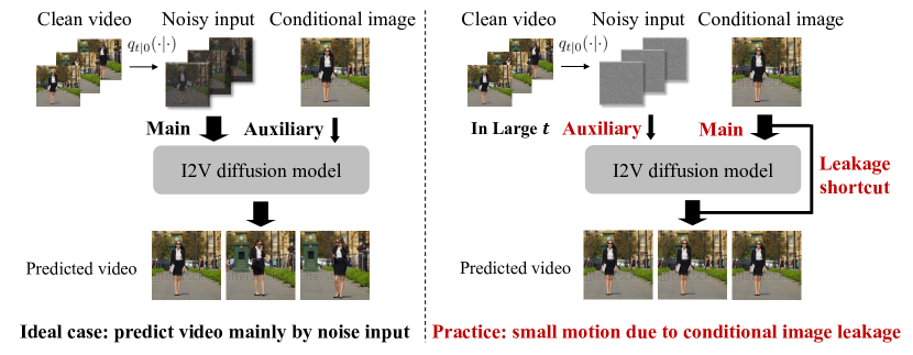
Figure 1: Schematic diagram of conditional image leakage. Ideally, I2V-DMs predict clean videos from noisy inputs, using the conditional image as auxiliary content guidance. However, at large time steps, the heavily corrupted input retains minimal video detail, causing the model tends to over-rely on the detailed conditional image and neglect the crucial task of synthesizing video from noisy inputs.

In this paper, we identify a significant but previously overlooked issue in the image-to-video diffusion models (I2V-DMs), namely, conditional image leakage (see Sec. 3.1). Ideally, the I2V-DMs should predict the added noise or clean video mainly from noisy inputs, with the conditional image serving as auxiliary guidance. However, as the diffusion process progresses—especially at large time steps, the heavily corrupted input retains minimal video detail, while the conditional image preserves extensive detail of the target video. This biases the model to over-rely on the conditional image while neglecting the essential task of synthesizing video from noisy inputs, leading to videos lacking dynamic and vivid motion. For instance, I2V-DMs that take a shortcut by directly replicating the conditional image may even achieve a lower loss. To validate this issue, we corrupt a ground truth (GT) clean video data using the forward transition kernel and compute one-step clean video predictions across all time steps. As illustrated in Fig. 2, predicted clean videos exhibit markedly reduced motion than GT at large time steps, with videos becoming almost entirely static at the final step.

Based on the analysis, we attempt to address the challenge in both inference and training. First, we present a simple yet effective training-free inference strategy, where we start the video generation process from an earlier time step instead of the final one, thus avoiding the unreliable late-time steps of the I2V-DMs (see Sec. 4.1). To further enhance performance, we derive an initial noise distribution with optimal analytic expressions (Analytic-Init) by minimizing the KL divergence between it and the actual marginal distribution to bridge the training-inference gap. Second, to mitigate the conditional image leakage during training, we introduce a time-dependent noise distribution (TimeNoise) that interferes with the conditional image, particularly at large time steps (Sec. 4.2). In principle, the distribution should favor high noise levels at large time steps to sufficiently disrupt the conditional image, then gradually decrease the noise levels as the time step diminishes. To achieve this, we utilize a logit-normal distribution with a center that monotonically increases over time and conduct a systematic analysis of its two hyperparameters. Notably, our strategies are designed to be plug-and-play, making them adaptable to various I2V-DMs based on both VP-SDE [12, 54] and VE-SDE [9] frameworks. Finally, the clean videos predicted by our method maintain motion dynamics comparable to the GT across all time steps, indicating the absence of conditional image leakage (see Fig. 6).

Empirically, we validate our methods on various I2V-DMs [9, 54, 12] using our collected open-domain images (ImageBench) and the UCF101 dataset. We conduct a user study on the ImageBench and report FVD [49] and IS [7] on UCF101. Extensive experimental results demonstrate that our strategies outperform baselines by producing videos with markedly more dynamic and natural motion, all while maintaining image alignment and temporal consistency.

2 Background

Diffusion Models.

Diffusion models gradually perturb data ${\bm{x}}_{0}\sim q({\bm{x}}_{0})$ through a forward diffusion process and reserve it to recover the data. The forward transitional kernel $q_{t|0}({\bm{x}}_{t}|{\bm{x}}_{0})$ is given by

$${\bm{x}}_{t}=\alpha_{t}{\bm{x}}_{0}+\sigma_{t}{\bm{\epsilon}},\quad{\bm{\epsilon}}\sim{\mathcal{N}}({\bm{0}},{\bm{I}}),\quad t\in[0,T],$$ (1)

where $\alpha_{t}$ and $\sigma_{t}$ are the noise schedule and chosen to ensure that ${\bm{x}}_{T}$ contains minimal information about ${\bm{x}}_{0}$. Two prevalent types of forward stochastic differential equation (SDEs) are commonly used [44, 28]. One is the variance-preserving SDE (VP-SDE) [40, 23], where $\alpha_{t}^{2}+\sigma_{t}^{2}=1$ with $\alpha_{t}\rightarrow 0$ as $t\rightarrow T$, ensuring $p_{T}({\bm{x}}_{T})=\mathcal{N}({\bm{0}},{\bm{I}})$. The other is the variance exploding SDE (VE-SDE), where $\alpha_{t}=1$ and $\sigma_{T}$ is set to a large constant, resulting in $p_{T}({\bm{x}}_{T})={\mathcal{N}}({\bm{0}},\sigma_{T}^{2}{\bm{I}})$. Such models can be parameterized using a noise-prediction model $\epsilon_{\theta}({\bm{x}}_{t},t)$ (${\bm{\epsilon}}$-prediction) [23] to optimize:

$$\mathbb{E}_{{\bm{x}}_{0}\sim q({\bm{x}}_{0}),{\bm{\epsilon}}\sim{\mathcal{N}}({\bm{0}},{\bm{I}}),t\sim\mathcal{U}(1,T)}\left[\|{\bm{\epsilon}}_{\theta}({\bm{x}}_{t},t)-{\bm{\epsilon}}\|_{2}^{2}\right],$$ (2)

where the noisy input ${\bm{x}}_{t}\sim q_{t|0}({\bm{x}}_{t}|{\bm{x}}_{0})$. Alternative parametrizations such as ${\bm{x}}_{0}$-prediction [28], ${\bm{v}}$-prediction [41], $F$-prediction [27] are also commonly used. The ${\bm{\epsilon}}$-prediction and ${\bm{x}}_{0}$-prediction loss aims to predict the added noise or clean video from noisy input ${\bm{x}}_{t}$. Starting from ${\bm{x}}_{T}\sim p_{T}({\bm{x}}_{T})$, various samplers [43, 32, 33, 27] can be employed to generate data.

Diffusion Models for Image-to-Video Generation.

Given any image ${\bm{y}}_{0}$ from the open domain, the goal of I2V is to generate a video $X_{0}=\{{\bm{x}}_{0}^{i}\}_{i=1}^{N}$ with dynamic and natural motion while maintaining the appearance of ${\bm{y}}_{0}$. This task can be formulated as designing a conditional distribution $p_{\theta}(X_{0}|{\bm{y}}_{0})$, which be achieved by a conditional diffusion model:

$$\mathbb{E}_{X_{0},{\bm{y}}_{0},{\bm{\epsilon}},t}\left[\|{\bm{\epsilon}}_{\theta}(X_{t},{\bm{y}}_{0},t)-{\bm{\epsilon}}\|_{2}^{2}\right],$$ (3)

where $X_{t}\sim q_{t|0}(X_{t}|X_{0})$. Typically, ${\bm{y}}_{0}$ is the first frame of $X_{0}$ and DynamiCrafter [54] adopts a randomly selected frame from $X_{0}$ as ${\bm{y}}_{0}$. The key issue is effectively integrating the conditional image ${\bm{y}}_{0}$ into the diffusion model. Most methods use CLIP image embeddings [39] to maintain the semantic content of ${\bm{y}}_{0}$. Notably, VideoCrafter1 [12] and Dynamicrafter [54] employ the last layer’s full patch visual tokens from the CLIP ViT, enriching the encoded information, and other approaches prefer the class token layer. Yet, solely depending on these embeddings, such as in VideoCrafter1 [12], compromises detail retention, impacting image alignment. To enhance detail representation, I2VGen-XL [58] combines the conditional image with the noisy initial frame, while VideoComposer [51] develops a STC-encoder for multiple conditions. Although superior to CLIP image embeddings, these strategies still fail to fully retain the conditional image content. To mitigate this, AnimateAnything [15], Dynamicrafter [54] and SVD [9] choose to directly concatenate noisy video $X_{t}$ with ${\bm{y}}_{0}$, which provides detailed information.

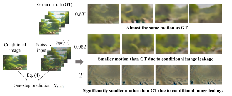
Figure 2: Identifying conditional image leakage in I2V-DMs. We corrupt a ground truth (GT) clean video and use it to compute $\hat{X}_{t\rightarrow 0}$ prediction across time steps. As time progresses, $\hat{X}_{t\rightarrow 0}$ exhibits markedly reduced motion than GT, with the videos becoming nearly static at the final step $T$, suggesting the existence of conditional image leakage in a large time step.

3 Conditional Image Leakage

In this section, we first identify a commonly overlooked issue in I2V-DMs: conditional image leakage, discussed in Sec. 3.1. We then discuss existing I2V-DMs with respect to this issue in Sec. 3.2.

3.1 Identifying Conditional Image Leakage in Image-to-video Diffusion Models

Although existing I2V-DMs discussed in Sec. 2 have obtained significant progress, such models are not fully understood. This section revisits and underscores a critical yet previously overlooked issue: conditional image leakage (CIL). As shown in Fig. 1, ideally, I2V-DMs should predict the added noise ($\epsilon$-prediction) or clean video (${\bm{x}}_{0}$-prediction) mainly from noisy input $X_{t}$, using the conditional image ${\bm{y}}_{0}$ as auxiliary content guidance. However, as the diffusion process progresses—particularly at large time steps, the heavily corrupted input $X_{t}$ contains minimal information about $X_{0}$, making it challenging to predict clean frames. Meanwhile, the conditional image retains considerable detail of $X_{0}$. This biases the model to over-rely on the conditional image while neglecting the essential task of synthesizing video from noisy inputs. For instance, a diffusion model that takes a shortcut by directly replicating ${\bm{y}}_{0}$ can even achieve a lower loss than one that accurately predicts the clean video from a heavily corrupted $X_{t}$. As a result, the synthesized videos lack dynamic and vivid motion. Notably, recent strategies that involve adjusting the noise schedule towards more noise [14, 26, 9, 31] may further exacerbate this issue (see details in Appendix C).

To validate this issue, we corrupt a ground truth (GT) clean video $X_{0}$ using the forward transition kernel in Eq. (1) and use it as the noisy input to compute the one-step prediction $\hat{X}_{t\rightarrow 0}$ at time $t$:

$$\hat{X}_{t\rightarrow 0}=\left(X_{t}-\sigma_{t}{\bm{\epsilon}}_{\theta}(X_{t},y,t)\right)/\alpha_{t}.$$ (4)

Ideally, $\hat{X}_{t\rightarrow 0}$ attempts to predict the GT $X_{0}$ from noisy input $X_{t}$ and exhibit comparable motion dynamics. However, as shown in Fig. 2, as time progresses—particularly at large time steps, $\hat{X}_{t\rightarrow 0}$ exhibits markedly reduced motion than GT, with the videos becoming nearly static at the final step $T$, suggesting the existence of the conditional image leakage. Consequently, it will generate an almost still video starting from $T$ by duplicating the conditional image (see Fig. 6).

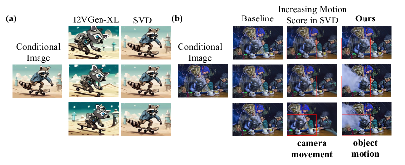
Figure 3: Understanding exiting work from conditional image leakage. (a) I2VGen-XL [58] mitigates the leakage at the expense of image alignment. (b) Increasing the SVD motion score induces unnatural camera movements with stationary objects. Our inference strategy, however, produces dynamic and natural motion in both people and the teapot.

3.2 Understanding Existing Work from Conditional Image Leakage

We now examine three popular I2V-DMs with respect to conditional image leakage: I2VGEN-XL [58], Dynamicrafter [54], and SVD [9]. Although these models do not explicitly address conditional image leakage, we believe their strategies may mitigate it to some extent.

Firstly, I2VGEN-XL [58] adds ${\bm{y}}_{0}$ with the first frame of noisy input, which reduces information about ${\bm{y}}_{0}$ largely and thus mitigates the leakage issue. However, Fig. 3(a) indicates that the generated videos do not accurately preserve ${\bm{y}}_{0}$. Dynamicrafter [54] and SVD [9] directly feed ${\bm{y}}_{0}$ into I2V-DMs, enhancing detail preservation but also facilitating leakage. Dynamicrafter selectively refines spatial layers while preserving the pre-trained temporal layers, which contain motion priors and thus maintain motion dynamics to a certain extent. However, it does not inherently solve the leakage issue. SVD [9] introduces an additional motion score to compel the model to generate videos with motion to align with motion score, thereby reducing reliance solely on ${\bm{y}}_{0}$ and mitigating conditional image leakage. However, we argue that it does not address the fundamental challenge facing I2V-DMs, where I2V-DMs should generate clean video primarily from noisy input. An example in Fig. 3(b) highlights this limitation. By increasing the motion score, the method produces videos with significant camera movement to meet the scalar motion score but leaves objects static. In contrast, the strategy we propose in Sec. 4.1 results in a video with vivid and naturalistic movement, where both the people and the teapot exhibit dynamic motion, offering a more effective solution to the fundamental challenges of I2V-DMs. Furthermore, if an inappropriate motion score is provided during inference, the resulting video may exhibit unnatural motion or poor temporal consistency to match the given score (see Fig. 12 in the Appendix). In summary, despite efforts by these works to somewhat mitigate conditional image leakage, the issue persists, underscoring the ongoing need for further exploration.

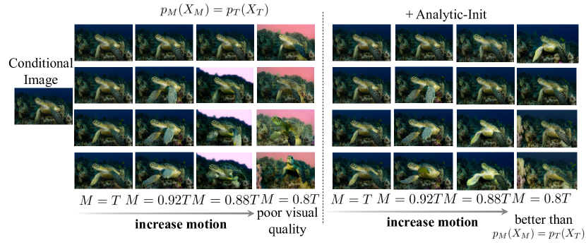
Figure 4: Benefits of tuning $M$ and Analytic-Init w.r.t. visual quality. An appropriate $M$ can enhance performance by increasing motion without compromising other performance. A too-small $M$ delivers poor visual quality due to the training-inference gap. Analytic-Init helps to mitigate it.

4 Solving Conditional Image Leakage in Image-to-video Diffusion Models

In this section, we tackle the issue of conditional image leakage from two perspectives: first, by outlining a training-free inference strategy to mitigate it, and second, by presenting a training strategy designed to rectify this phenomenon during the training phase.

4.1 Inference Strategy

As discussed in Sec. 3.1, conditional image leakage commonly occurs at large time steps. To address it, a straightforward solution is to start the generation process from an earlier time step $M\in[0,T]$, avoiding the unreliable later stages of I2V-DMs. Let $p_{M}(X_{M})$ denote the initial noise distribution at the start time $M$. Initially, we set $p_{M}(X_{M})=p_{T}(X_{T})$, i.e. ${\mathcal{N}}({\bm{0}},{\bm{I}})$ in VP-SDE [23] or ${\mathcal{N}}({\bm{0}},\sigma_{T}^{2}{\bm{I}})$ in VE-SDE [28]. As illustrated in the third column ($M=0.92T$) of Fig. 4, this straightforward strategy markedly improves motion dynamics without sacrificing other performance. However, a smaller $M$ value (e.g., $M=0.8T$) hurts the visual quality due to the training-inference discrepancy.

To bridge the training-inference gap, we propose to minimize the KL divergence between the initial noise distribution $p_{M}(X_{M})$ and the actual marginal distribution of the diffusion process at time $M$, denoted as $q_{M}(X_{M})$. Inspired by existing work [4, 3, 55], when $p_{M}(X_{M})$ is modeled as a normal distribution ${\mathcal{N}}(X_{M};{\bm{\mu}}_{p},\sigma_{p}^{2}{\bm{I}})$, we derive analytical expressions for the optimal mean ${\bm{\mu}}_{p}^{*}$ and variance $\sigma_{p}^{2\ast}$ as follows. We refer to it as the Analytic Noise Initialization (Analytic-Init).

Proposition 1.

Given a normal distribution $p_{M}(X_{M})={\mathcal{N}}(X_{M};{\bm{\mu}}_{p},\sigma_{p}^{2}{\bm{I}})$ and $q_{M}(X_{M})$ is the margin distribution of diffusion forward process at time $M$, with the forward trainsition kernel $q_{M|0}(X_{M}|X_{0})={\mathcal{N}}(X_{M};\alpha_{M}X_{0},\sigma_{M}^{2}{\bm{I}})$, the minimization problem $\underset{{\bm{\mu}}_{p},\sigma_{p}^{2}}{\min}D_{KL}(q_{M}(X_{M})||p_{M}(X_{M}))$ yields the following optimal solution:

$${\bm{\mu}}_{p}^{*}=\alpha_{M}\mathbb{E}_{q(X_{0})}[X_{0}],\quad\sigma_{p}^{2\ast}=\alpha_{M}^{2}\frac{\sum_{j=1}^{d}[Var(X_{0}^{(j)})]}{d}+\sigma_{M}^{2},$$ (5)

where $q(X_{0})$ denotes the data distribution , $d$ denotes the dimension of the data, and $X_{0}^{(j)}$ denotes the j-th component of $X_{0}$.

Appendix A provides detailed proof of Proposition 1. Empirically, we can estimate ${\bm{\mu}}_{p}^{*}$ and $\sigma_{p}^{2\ast}$ using the method of moments [4]. Compared with the naive approach where $p_{M}(X_{M})=p_{T}(X_{T})$, Analytic-Init can achieve superior visual quality by reducing the training-inference gaps, especially with a smaller $M$. The theoretical insights and Proposition 1 are validated by the results in Tab. 4, measured by the commonly used FVD and IS metrics.

Figure 5: Effects of tuning $\mu(t)$ and $\beta_{m}$ in TimeNoise. Adjusting these parameters allows for a flexible trade-off between dynamic motion and image alignment. Higher noise levels result in more pronounced motion but reduced image alignment.

Figure 6: Effectiveness of TimeNoise to address conditional image leakage. We replicate the experiments described in Sec. 3.1 to evaluate TimeNoise. Applying TimeNoise ensures that $\hat{X}_{t\rightarrow 0}$ maintains motion dynamics comparable to the GT across all time steps, indicating the absence of conditional image leakage. Consequently, we can generate videos with high motion starting from $T$.

4.2 Training Strategy

The previous section explores strategies to mitigate conditional image leakage during inference. This section presents methods to address this issue during the training phase. As noted in Sec. 3.1, the conditional image ${\bm{y}}_{0}$ remains informative of the target video, leading I2V-DMs to depend excessively on it. Therefore, an intuitive idea is to perturb ${\bm{y}}_{0}$ to relieve the reliance on it.

Our first attempt is to introduce noise similar in scale to that used in $X_{t}$. This aims to equalize the model’s challenge in predicting clean video from $X_{t}$ or ${\bm{y}}_{t}$, reducing its dependency on ${\bm{y}}_{0}$. However, this strategy also makes it difficult to harness ${\bm{y}}_{0}$, resulting in lower video quality. To overcome this, we propose a noise distribution on ${\bm{y}}_{0}$ that introduces substantial noise to prevent leakage while maintaining a cleaner ${\bm{y}}_{0}$ to aid content generation. As discussed earlier, as time progresses, $X_{t}$ becomes less informative about $X_{0}$, increasing the risk of leakage. This insight leads us to develop a time-dependent noise distribution $p_{t}(\beta_{s})$ (TimeNoise). The design principle is to favor high noise levels at large time steps to sufficiently disrupt ${\bm{y}}_{0}$, shifting towards lower noise levels as the time step decreases. To achieve this, we employ a logit-normal distribution [18, 1] defined as below:

$$p_{t}(\beta_{s};\mu(t),\beta_{m})=\frac{\beta_{m}}{\sqrt{2\pi}}\frac{1}{\beta_{s}(\beta_{m}-\beta_{s})}e^{-\frac{(\text{logit}(\frac{\beta_{s}}{\beta_{m}})-\mu(t))^{2}}{2}},$$ (6)

where $\text{logit}(\frac{\beta_{s}}{\beta_{m}})$ follows a normal distribution centered around $\mu(t)$ with a standard deviation of 1. Our noise distribution includes two hyperparameters: $\beta_{m}$, the maximum noise level, and $\mu(t)$, the center of the distribution. As illustrated in Fig. 8(a), we can adhere to the previously stated design principle of $p_{t}(\beta_{s})$ by adjusting $\mu(t)$ over time $t$. Finally, the noisy conditional image ${\bm{y}}_{s}$ at time $t$ is obtained by ${\bm{y}}_{s}={\bm{y}}_{0}+\beta_{s}{\bm{\epsilon}}$, where $\beta_{s}\sim p_{t}(\beta_{s}),{\bm{\epsilon}}\sim{\mathcal{N}}({\bm{0}},{\bm{I}})$. We also tried other adding noise choices but found them to be less effective (see Appendix D).

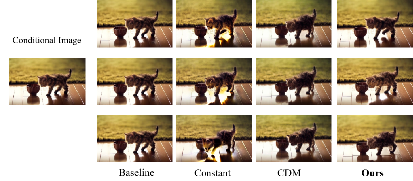
Figure 10: The qualitative comparison between our TimeNoise and baselines mentioned in Sec. 4.2. The constant results in poor image alignment, while the CDM [24] shows low motion. Ours achieves the best visual quality.

Next, we conduct a systematic analysis of two hyperparameters to investigate their impact on video generation. The first, $\mu(t)$, should ideally increase monotonically with time, where we set it ranging from $\mu(0)=-1$ to $\mu(T)=1$. We explore three typical functional forms for $\mu(t)$ (see Fig. 8(b)): (1) linear: $\mu(t)=2t-1$, (2) convex:$\mu(t)=2t^{a}-1$, where $a>1$ and (3) concave: $\mu(t)=2t^{a}-1$, where $a\in(0,1)$. As shown in Fig. 5(a), our TimeNoise strategy produces videos with more dynamic motion than the baseline. Functions that introduce higher noise levels, such as the concave function, enhance dynamic motion but reduce temporal consistency and image alignment. We also test the following baselines: (1) constant, where $\beta_{s}=\beta_{m}\frac{\mu(t)+1}{2}$ represents a single value rather than a distribution, and (2) a conditioning augmentation method from CDM [24]. Results indicate that the former method results in poor image alignment, while the latter shows low motion (see Fig. 10 in the Appendix). We then examine the maximum noise level, $\beta_{m}$. As shown in Fig. 5(b), a higher $\beta_{m}$ enhances dynamic motion but decreases temporal consistency and image alignment, while a lower $\beta_{m}$ leads to less motion. Considering that VideoCrafter1 and DynamiCrafter utilize full patch visual tokens from CLIP, not just the class token, we also apply noise to these tokens. Finally, we replicated the experiments outlined in Sec. 3.1, and the results depicted in Fig. 6 demonstrate that our TimeNoise ensures $\hat{X}_{t\rightarrow 0}$ maintains motion dynamics comparable to the ground truth across all time steps. This indicates an absence of conditional image leakage, underscoring the effectiveness of our approach.

Figure 7: Visualizing the effectiveness of our inference and training strategies. Ours significantly enhances video dynamism while maintaining image alignment and temporal consistency. VC. and DC. denote VideoCrafter1 [12] and DynamiCrafter [54] respectively.

5 Related Work

Diffusion Models for Image Generation.

Recently, diffusion models have recently achieved significant breakthroughs in image, video, and 3D generation [23, 16, 40, 37, 5, 59, 36, 52, 53, 60]. For image generation, the latent diffusion model [40] addresses computational costs by leveraging VQ-VAE [47] to transform pixel-space images into compact latent representations, subsequently training diffusion models within this latent space. Building upon the latent space concept, subsequent works such as SDXL [38], DALLE-3 [8], and SD3 [18] have further enhanced performance. Exploiting these advancements in text-to-image diffusion models, numerous methods have demonstrated promising results in text-driven controllable image generation and image editing [57, 21, 46]. In image editing, studies such as Prompt-to-Prompt [21] and Plug-and-Play [46] have explored attention-based control mechanisms over generated content, consistently delivering impressive results. For image translation, EGSDE [59] and DiffuseIT [29] propose to employ an additional energy function to guide the inference process of a pre-trained diffusion model.

Diffusion Models for T2V Generation.

Approaches to T2V generation can be classified into two main categories. The first category involves directly generating videos based on text [42, 10, 22, 12, 13, 48, 56, 50, 9, 17]. For instance, as a pioneering endeavor, Make-A-Video [42] utilizes a pre-trained text-to-image model along with a prior network for T2V diffusion models, obviating the necessity for paired video-text datasets. VideoLDM [10] maintains the parameters of a pre-trained T2I model while fine-tuning newly introduced temporal layers. More recently, transformers have emerged as a foundational architecture for video generation due to their scalability [20, 35, 34]. The second category typically entails a two-step generation process: first generating an image based on the textual input and subsequently creating a video conditioned on the text and the generated image [30, 19]. For instance, Emu-video [19] initializes a factorized text-to-video model using a pre-trained text-to-image model and then fine-tunes temporal modules in the I2V stage.

tablePerformance on the UCF101 dataset. Method-finetune denotes our fine-tuned version. Method-CIL denotes the full version using both inference and training strategies. Model FVD$\downarrow$ IS$\uparrow$ DymiCrafter [13] 363.8 16.39 + Analytic-Init (M=0.96T) 316.3 17.66 DymiCrafter-finetune 382.5 21.12 + Analytic-Init (M=0.96T) 342.9 22.71 + TimeNoise 334.9 21.42 DymiCrafter-CIL 332.1 22.84 VideoCrafter1 [12] 353.9 18.75 + Analytic-Init (M=0.96T) 341.6 19.86 VideoCrafter1-finetune 460.3 23.98 + Analytic-Init (M=0.96T) 450.1 24.50 + TimeNoise 452.2 24.62 VideoCrafter1-CIL 443.7 25.11 SVD [9] ($\sigma_{T}=700$) 388.3 36.32 + Analytic-Init ($\sigma_{M}=100$) 382.0 36.81 SVD-finetune 311.0 22.03 + Analytic-Init ($\sigma_{M}=100$) 277.1 22.18 + TimeNoise 272.2 23.01 SVD-CIL 272.4 25.18

Figure 8: (a)Visualization of designed noise distribution. Adjusting $\mu(t)$ over time $t$ can satisfy the design principle. For example, set large $\mu(t)$ for large $t$ (purple curve) and small $\mu(t)$ for small $t$ (blue curve). (b)Visualization of different $\mu(t)$.

6 Experiments

Datasets and Evaluation Metrics.

We validate our training strategy on the WebVid-2M dataset [2], resizing and center-cropping all videos to $320\times 512$ with 16 frames. For evaluation, we validate our methods on UCF101 and our collected ImageBench, comprising 100 images from various websites and T2I models like SDXL [38] and UniDiffuser [5], covering categories like nature, humans, and more for comprehensive evaluation. For ImageBench, we conduct user studies with 10 subjects to perform pairwise comparisons of our methods against baselines, evaluating motion, temporal consistency, image alignment, and overall performance. On UCF101, we report Fréchet Video Distance (FVD) and Inception Score (IS). Further details can be found in Appendix B.

Implementation Details.

For Analytic-Init, we use 5000 samples from the Webvid-2M dataset to estimate $p_{M}(X_{M})$ by default. We set $M=0.96T,0.96T$ and $\sigma_{M}=100$ for VideoCrafter1 [12], DynamiCrafter [54], and SVD [9] on UCF101. For ImageBench, we adjust $M$ to $0.92T,0.92T$ and $\sigma_{M}=100$. For the TimeNoise, we set $\beta_{m}=25,100$, and $100$ for VideoCrafter1, DynamiCrafter, and SVD, respectively. The function $\mu(t)=2t^{5}-1$ is applied across all baselines. These baselines are fine-tuned for 20,000 iterations, using either the official code or a replication of the official settings except for batch size. More detailed information can be found in the Appendix B.

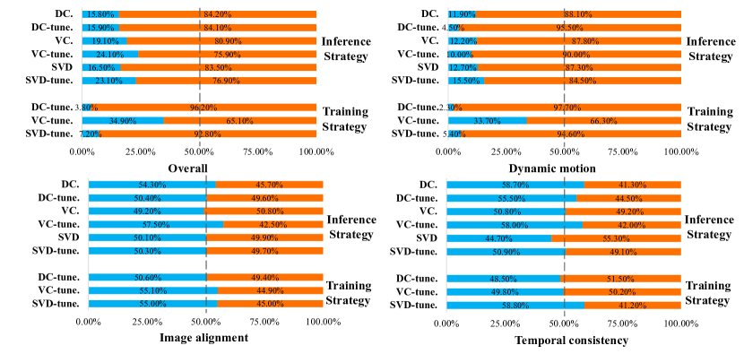
Figure 9: User preference for ours against baselines. DC. and VC. denote DynamiCrafter and VideoCrafter1 [12]. Method-finetune denotes our fine-tuned version. Ours significantly enhances video dynamics without compromising temporal consistency and image alignment (around 50$\%$). Overall, ours achieves superior results.

6.1 Results

The effectiveness of our inference and training strategy.

We validate our strategies on three I2V-DMs: VideoCrafter1 [12], DynamiCrafter [54], and SVD [48]. Demonstrated in Fig. 7, our strategies significantly enhance video dynamism and natural motion, all while maintaining image alignment and temporal consistency. The findings are corroborated by the user study in Fig. 9. Considering overall aspects, ours achieves superior results. Tab. 8 showcases the quantitative superiority of our inference and training strategies, which outperform all baselines significantly. For instance, on DynamiCrafter [54], we improve the FVD score by 47.5 and 47.6 using our inference and training strategy respectively, suggesting the effectiveness of our method.

Evaluating the combined inference and training strategies.

In this section, we aim to investigate the necessity of combining two strategies. As illustrated in Tab. 3, for DynamiCrafter [54] and SVD [9], our TimeNoise effectively mitigates conditional image leakage, rendering the additional inference strategy less impactful. Conversely, for VideoCrafter1 [12], which relies solely on CLIP image embedding for information, employing excessive TimeNoise disrupts image alignment. Hence, we utilize a moderate TimeNoise ($\beta_{m}=25$), where the inference strategy remains effective.

7 Conclusions and Discussions

In this paper, we identify a common issue in I2V-DMs: conditional image leakage. We address this challenge from two aspects. First, we introduce a training-free inference strategy that starts the generation process from an earlier time step to avoid the unreliable late-time steps of I2V-DMs. Second, we design a time-dependent noise distribution for the conditional image to mitigate conditional image leakage during training. We validate the effectiveness of these strategies across various I2V-DMs.

Limitations and broader impact.

One limitation of this paper is the need to balance time-dependent noise distribution to prevent conditional image leakage while maintaining image integrity. While we demonstrate the effectiveness of our training strategy on existing image-to-video diffusion models, we do not provide a definitive noise distribution choice for a scratch-trained model. We leave this in the future work. Furthermore, we must use the method responsibly to prevent any negative social impacts, such as the creation of misleading fake videos.

Appendix A Proof of Proposition 1

According to Lemma 2 of Analytic-DPM [4], the KL divergence between initial noise distribution $p_{M}(X_{M})$ and the actual marginal distribution $q_{M}(X_{M})$ can be expressed as:

$$D_{KL}(q_{M}(X_{M})||p_{M}(X_{M}))=D_{KL}({\mathcal{N}}(X_{M};{\bm{\mu}}_{q},\Sigma_{q})||p_{M}(X_{M}))$$

$$+H({\mathcal{N}}(X_{M};{\bm{\mu}}_{q},\Sigma_{q}))-H(q_{M}(X_{M})),$$ (7)

where ${\bm{\mu}}_{q},\Sigma_{q}$ denote expectation and covariance matrix of $q_{M}(X_{M})$, and $H(\cdot)$ denotes the entropy of a distribution. Since $q_{M}(X_{M})$ is independent of $p_{M}(X_{M})$, the last two terms can be considered as constants. Therefore, minimizing the Eq. (A) is equivalent to minimizing $D_{KL}(N(X_{M};{\bm{\mu}}_{q},\Sigma_{q})||p_{M}(X_{M}))$. For normal distributions, $D_{KL}(N(X_{M};{\bm{\mu}}_{q},\Sigma_{q})||p_{M}(X_{M}))$ could be expanded as:

$$\frac{1}{2}[({\bm{\mu}}_{q}-{\bm{\mu}}_{p})^{T}\Sigma_{p}^{-1}({\bm{\mu}}_{q}-{\bm{\mu}}_{p})-\log\det(\Sigma_{p}^{-1}\Sigma_{q})+tr(\Sigma_{p}^{-1}\Sigma_{q})-d],$$ (8)

$$=\frac{1}{2}[\frac{1}{\sigma_{p}^{2}}\lVert{\bm{\mu}}_{p}-{\bm{\mu}}_{q}\rVert^{2}+d\log(\sigma_{p}^{2})+\frac{1}{\sigma_{p}^{2}}tr(\Sigma_{q})-\log\det(\Sigma_{q})-d],$$ (9)

where $d$ denotes the dimension of the data. Minimizing Eq. (9) yields:

$${\bm{\mu}}_{p}^{*}={\bm{\mu}}_{q}=\mathbb{E}_{q_{M}(X_{M})}[X_{M}].$$ (10)

Taking the derivative of Eq. 9 with respect to $\sigma_{p}^{2}$, we can obtain

$$\sigma_{p}^{2\ast} =\frac{trCov_{q_{M}(X_{M})[X_{M}]+\lVert{\bm{\mu}}_{p}-{\bm{\mu}}_{q}\rVert^{2}}}{d},$$ (11)

$$=\frac{trCov_{q_{M}(X_{M})[X_{M}]}}{d},$$ (12)

$$=\frac{\sum_{j=1}^{d}(Var(X_{M}^{(j)}))}{d}.$$ (13)

Taking the $X_{M}$ defined in Eq. (1) into Eq. (10), the optimal ${\bm{\mu}}_{p}^{*}$ could be further represented as

$$\mu_{p}^{*} =\alpha_{M}\mathbb{E}_{q(X_{0})}[X_{0}]+\mathbb{E}_{q({\bm{\epsilon}})}[{\bm{\epsilon}}],$$ (14)

$$=\alpha_{M}\mathbb{E}_{q(X_{0})}[X_{0}].$$ (15)

Similarly, for the optimal variance $\sigma_{p}^{2\ast}$, we can derive

$$Var(X_{M}^{(j)})=Var(\alpha_{M}X_{0}^{(j)}+\sigma_{M}{\bm{\epsilon}}^{(j)})$$ (16)

Given that $X_{0}$ and ${\bm{\epsilon}}$ are independent of each other, the variance $Var(X_{M}^{(j)})$ can be decomposed further:

$$Var(X_{M}^{(j)}) =Var(\alpha_{M}X_{0}^{(j)})+Var(\sigma_{M}{\bm{\epsilon}}^{(j)}),$$ (17)

$$=\alpha_{M}^{2}Var(X_{0}^{(j)})+\sigma_{M}^{2}.$$ (18)

Finally, taking Eq. (18) into Eq. (13), the optimal $\sigma_{p}^{2\ast}$ can be represented as

$$\sigma_{p}^{2\ast}=\alpha_{M}^{2}\frac{\sum_{j=1}^{d}[Var(X_{0}^{(j)})]}{d}+\sigma_{M}^{2}.$$ (19)

Appendix B Implementation Details

Table 1: Code Links and Licenses.

Method	Link	License
VideoCrafter1 [12]	https://github.com/AILab-CVC/VideoCrafter	Apache License
DynamiCrafter [54]	https://github.com/Doubiiu/DynamiCrafter	Apache License
SVD	https://github.com/Stability-AI/generative-models	MIT License
UniDiffusers [5]	https://github.com/thu-ml/unidiffuser	AGPL-3.0 license
SDXL	https://github.com/Stability-AI/generative-models	Open RAIL++-M

B.1 Code Used and License

We validate our strategies on DynamiCrafter [54] ($320\times 512$ version), VideoCrafter1 [12] ($320\times 512$ version), and SVD [9]. All used codes in this paper and their licenses are listed in Tab. 1.

B.2 Training and Inference Details

We utilize the official training code of DynamiCrafter (refer to Tab. 1) to fine-tune both DynamiCrafter [54] and VideoCrafter1 [12], and reproduce the training code for SVD by ourselves. Throughout the training phase, we maintained consistent settings across all models, with the sole exception of incorporating our TimeNoise component for a fair comparison. Each model was fine-tuned using the WebVid-2M dataset [2], where videos were resized and center-cropped to dimensions of $320\times 512$ and segmented into sequences of 16 frames. In light of the discussions in Sec. 3.2 regarding the adverse effects of motion scores and the lack of a precise method by SVD [9] to compute these scores, we set a fixed motion score of $20$ during training. We fix the frame rate at $3$ fps and use dynamic frame rates for DynamiCrafter [54] and VideoCrafter1 [12]. Additional details can be found in Tab. B.2 and Tab. B.2. Our experiments were conducted using A800-80G GPUs, and the computational costs are detailed in Tab. 2. For inference, the official model codes were used for sampling (see Tab. 1). Specifically, we employed a DDIM sampler with 50 steps for DynamiCrafter [54] and VideoCrafter1 [12], and Heun’s 2nd order method with 25 steps for SVD [9].

tableTraining settings for DynamiCrafter [54] and VideoCrafter1 [12]. Config Value Optimizer AdamW Learning rate 1e-5 Weight decay 1e-2 Optimizer momentum $\beta_{1},\beta_{2}$=0.9, 0.999 Batch size 64 Training iterations 20,000

tableTraining settings for SVD [9]. Config Value Optimizer AdamW Learning rate 3e-5 Weight decay 1e-2 Optimizer momentum $\beta_{1},\beta_{2}$=0.9,0.999 Batch size 48 Training iterations 20,000

Table 2: Compute resources.

Model	Iterations	GPU-type	GPU-nums	Hours
DynamiCrafter [54]	20,000	A800	8	8
VideoCrafter1 [12]	20,000	A800	8	8
SVD [9]	20,000	A800	6	7

B.3 Evaluation

FVD and IS. Following prior studies [25, 10], we compute the Fréchet Video Distance (FVD) and Inception Score (IS) for 2,048 and 10,000 samples on the UCF101 dataset, respectively. Specifically, the FVD is calculated using the code available at https://github.com/SongweiGe/TATS/ with a pre-trained I3D action classification model, which can be accessed at https://www.dropbox.com/scl/fi/c5nfs6c422nlpj880jbmh/i3d_torchscript.pt?rlkey=x5xcjsrz0818i4qxyoglp5bb8&dl=1. The IS is derived using the code from https://github.com/pfnet-research/tgan2, employing a pre-trained C3D model [45]. For this process, we sample 16 frames at 3 fps, resize them to the default resolution of each model, and use the first frame as the conditional image to generate videos. The FVD and IS are then computed between the generated videos and the ground truth videos. For DynamiCrafter [54] and VideoCrafter1 [12], which utilize text as an additional condition, we employ categories as the textual input.

User study. We ask users to compare ours with the baselines and determine which ones exhibit more dynamic and natural motion, greater temporal consistency, better alignment with the conditional image, and overall preference.

Table 3: Evaluating the combined inference (Inference.) and training (Train.) strategies. Rat. denotes a user study that ranks methods. Refer to Sec. 6.1 for detailed analysis.

Inference.	Train.	VideoCrafter1 [12]			DynamiCrafter [54]			SVD [9]
		FVD$\downarrow$	IS$\uparrow$	Rat.$\downarrow$	FVD$\downarrow$	IS$\uparrow$	Rat.$\downarrow$	FVD$\downarrow$	IS$\uparrow$	Rat.$\downarrow$
✗	✗	460.3	23.98	4	382.5	21.12	4	311.0	22.03	4
✓	✗	450.1	24.50	1.9	342.9	22.71	2.9	277.1	22.18	2.9
✗	✓	452.2	24.62	2.7	334.9	21.42	1.4	272.2	23.01	1.6
✓	✓	443.7	25.11	1.4	332.1	22.84	1.7	272.4	25.18	1.5

Appendix C The Influence of Adjusting the Noise Schedule

In this section, we first examine commonly used strategies that involve adjusting the noise schedule to higher noise levels to bridge the training-inference gap [14, 26, 9, 31], which, unfortunately, may exacerbate conditional image leakage. Following the SVD [9], we increase noise by adjusting the $P_{mean}$ in the EDM framework [27]. Surprisingly, as shown in Fig. 11, we observe that larger $P_{mean}$ values correspond to reduced motion in the generated videos. We hypothesize that this is due to the increased noise added to $X_{t}$ by larger $P_{mean}$, making it more challenging to predict clean frames and thus more prone to conditional image leakage. Consequently, the synthesized videos tend to lack dynamic and vivid motion.

Appendix D Ablation Studies for Adding Noise Method

In this section, we show another choice to add noise to the conditional image. Specifically, the noisy conditional image ${\bm{y}}_{s}$ at time $t$ is obtained by

$${\bm{y}}_{s}=(1-\beta_{s}){\bm{y}}_{0}+\beta_{s}{\bm{\epsilon}},$$ (20)

where $\beta_{s}\sim p_{t}(\beta_{s}),{\bm{\epsilon}}\sim{\mathcal{N}}({\bm{0}},{\bm{I}})$, and $\beta_{m}=1$. As shown in Fig. 13, this choice leads to video discoloration in SVD [9].

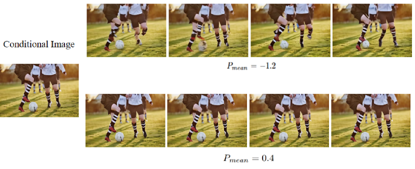
Figure 11: Adjusting the noise schedule towards more noise further exacerbate conditional image leakage.

Figure 12: An inappropriate motion score leads to poor temporal consistency.

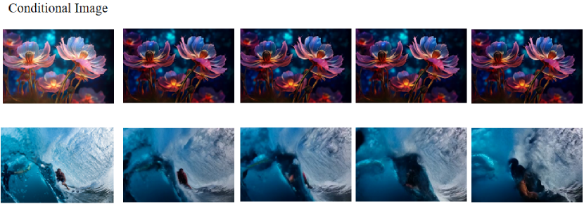
Figure 13: Other choice of adding noise on conditional image. Adding noise via Eq. 20 causes video discoloration in SVD [9].

Table 4: Effects of tuning $M$ and Analytic-Init.

Model	$M$	FVD$\downarrow$	IS$\uparrow$
DynamiCrafter [54]	T	363.8	16.39
	0.98T	345.1	16.57
	0.96T	343.1	17.54
	0.94T	325.2	19.12
	0.92T	365.8	20.49
	0.9T	442.2	22.81
DynamiCrafter + Analytic-Init	0.98T	324.3	16.44
	0.96T	316.3	17.66
	0.94T	319.6	19.13
	0.92T	347.2	20.58
	0.9T	378.6	22.40

Table 5: Quantitative results of the inference strategy across varying initial time $M$ on the UCF101 dataset.

Model	$M$	FVD$\downarrow$	IS$\uparrow$
DynamiCrafter [54]	T	363.8	16.39
+ Analytic-Init	0.96T	316.3	17.66
	0.92T	347.2	20.58
	0.88T	407.2	23.32
	0.84T	535.1	24.27
	0.8T	696.1	23.67
VideoCrafter1 [12]	T	353.9	18.75
+ Analytic-Init	0.96T	341.6	19.86
	0.92T	344.3	21.58
	0.88T	368.4	21.82
	0.84T	400.8	21.90
	0.8T	445.6	21.21
Model	$\sigma_{M}$	FVD$\downarrow$	IS$\uparrow$
SVD-finetune [9]	700	311.0	22.03
+ Analytic-Init	500	301.9	22.00
	300	290.2	21.94
	100	277.1	22.18
	70	272.5	22.27
	50	295.5	21.89

References

- [1] Jhon Atchison and Sheng M Shen. Logistic-normal distributions: Some properties and uses. Biometrika, 67(2):261–272, 1980.
- [2] Max Bain, Arsha Nagrani, Gül Varol, and Andrew Zisserman. Frozen in time: A joint video and image encoder for end-to-end retrieval. In Proceedings of the IEEE/CVF International Conference on Computer Vision, pages 1728–1738, 2021.
- [3] Fan Bao, Chongxuan Li, Jiacheng Sun, Jun Zhu, and Bo Zhang. Estimating the optimal covariance with imperfect mean in diffusion probabilistic models. arXiv preprint arXiv:2206.07309, 2022.
- [4] Fan Bao, Chongxuan Li, Jun Zhu, and Bo Zhang. Analytic-dpm: an analytic estimate of the optimal reverse variance in diffusion probabilistic models. arXiv preprint arXiv:2201.06503, 2022.
- [5] Fan Bao, Shen Nie, Kaiwen Xue, Chongxuan Li, Shi Pu, Yaole Wang, Gang Yue, Yue Cao, Hang Su, and Jun Zhu. One transformer fits all distributions in multi-modal diffusion at scale. arXiv preprint arXiv:2303.06555, 2023.
- [6] Fan Bao, Chendong Xiang, Gang Yue, Guande He, Hongzhou Zhu, Kaiwen Zheng, Min Zhao, Shilong Liu, Yaole Wang, and Jun Zhu. Vidu: a highly consistent, dynamic and skilled text-to-video generator with diffusion models. arXiv preprint arXiv:2405.04233, 2024.
- [7] Shane Barratt and Rishi Sharma. A note on the inception score. arXiv preprint arXiv:1801.01973, 2018.
- [8] James Betker, Gabriel Goh, Li Jing, Tim Brooks, Jianfeng Wang, Linjie Li, Long Ouyang, Juntang Zhuang, Joyce Lee, Yufei Guo, et al. Improving image generation with better captions. Computer Science. https://cdn. openai. com/papers/dall-e-3. pdf, 2(3):8, 2023.
- [9] Andreas Blattmann, Tim Dockhorn, Sumith Kulal, Daniel Mendelevitch, Maciej Kilian, Dominik Lorenz, Yam Levi, Zion English, Vikram Voleti, Adam Letts, et al. Stable video diffusion: Scaling latent video diffusion models to large datasets. arXiv preprint arXiv:2311.15127, 2023.
- [10] Andreas Blattmann, Robin Rombach, Huan Ling, Tim Dockhorn, Seung Wook Kim, Sanja Fidler, and Karsten Kreis. Align your latents: High-resolution video synthesis with latent diffusion models. In Proceedings of the IEEE/CVF Conference on Computer Vision and Pattern Recognition, pages 22563–22575, 2023.
- [11] Tim Brooks, Bill Peebles, Connor Holmes, Will DePue, Yufei Guo, Li Jing, David Schnurr, Joe Taylor, Troy Luhman, Eric Luhman, Clarence Ng, Ricky Wang, and Aditya Ramesh. Video generation models as world simulators. 2024.
- [12] Haoxin Chen, Menghan Xia, Yingqing He, Yong Zhang, Xiaodong Cun, Shaoshu Yang, Jinbo Xing, Yaofang Liu, Qifeng Chen, Xintao Wang, et al. Videocrafter1: Open diffusion models for high-quality video generation. arXiv preprint arXiv:2310.19512, 2023.
- [13] Haoxin Chen, Yong Zhang, Xiaodong Cun, Menghan Xia, Xintao Wang, Chao Weng, and Ying Shan. Videocrafter2: Overcoming data limitations for high-quality video diffusion models. arXiv preprint arXiv:2401.09047, 2024.
- [14] Ting Chen. On the importance of noise scheduling for diffusion models. arXiv preprint arXiv:2301.10972, 2023.
- [15] Zuozhuo Dai, Zhenghao Zhang, Yao Yao, Bingxue Qiu, Siyu Zhu, Long Qin, and Weizhi Wang. Animateanything: Fine-grained open domain image animation with motion guidance. arXiv e-prints, pages arXiv–2311, 2023.
- [16] Prafulla Dhariwal and Alexander Nichol. Diffusion models beat gans on image synthesis. Advances in neural information processing systems, 34:8780–8794, 2021.
- [17] Patrick Esser, Johnathan Chiu, Parmida Atighehchian, Jonathan Granskog, and Anastasis Germanidis. Structure and content-guided video synthesis with diffusion models. In Proceedings of the IEEE/CVF International Conference on Computer Vision, pages 7346–7356, 2023.
- [18] Patrick Esser, Sumith Kulal, Andreas Blattmann, Rahim Entezari, Jonas Müller, Harry Saini, Yam Levi, Dominik Lorenz, Axel Sauer, Frederic Boesel, et al. Scaling rectified flow transformers for high-resolution image synthesis. arXiv preprint arXiv:2403.03206, 2024.
- [19] Rohit Girdhar, Mannat Singh, Andrew Brown, Quentin Duval, Samaneh Azadi, Sai Saketh Rambhatla, Akbar Shah, Xi Yin, Devi Parikh, and Ishan Misra. Emu video: Factorizing text-to-video generation by explicit image conditioning. arXiv preprint arXiv:2311.10709, 2023.
- [20] Agrim Gupta, Lijun Yu, Kihyuk Sohn, Xiuye Gu, Meera Hahn, Li Fei-Fei, Irfan Essa, Lu Jiang, and José Lezama. Photorealistic video generation with diffusion models. arXiv preprint arXiv:2312.06662, 2023.
- [21] Amir Hertz, Ron Mokady, Jay Tenenbaum, Kfir Aberman, Yael Pritch, and Daniel Cohen-Or. Prompt-to-prompt image editing with cross attention control. arXiv preprint arXiv:2208.01626, 2022.
- [22] Jonathan Ho, William Chan, Chitwan Saharia, Jay Whang, Ruiqi Gao, Alexey Gritsenko, Diederik P Kingma, Ben Poole, Mohammad Norouzi, David J Fleet, et al. Imagen video: High definition video generation with diffusion models. arXiv preprint arXiv:2210.02303, 2022.
- [23] Jonathan Ho, Ajay Jain, and Pieter Abbeel. Denoising diffusion probabilistic models. Advances in neural information processing systems, 33:6840–6851, 2020.
- [24] Jonathan Ho, Chitwan Saharia, William Chan, David J Fleet, Mohammad Norouzi, and Tim Salimans. Cascaded diffusion models for high fidelity image generation. Journal of Machine Learning Research, 23(47):1–33, 2022.
- [25] Wenyi Hong, Ming Ding, Wendi Zheng, Xinghan Liu, and Jie Tang. Cogvideo: Large-scale pretraining for text-to-video generation via transformers. arXiv preprint arXiv:2205.15868, 2022.
- [26] Emiel Hoogeboom, Jonathan Heek, and Tim Salimans. simple diffusion: End-to-end diffusion for high resolution images. In International Conference on Machine Learning, pages 13213–13232. PMLR, 2023.
- [27] Tero Karras, Miika Aittala, Timo Aila, and Samuli Laine. Elucidating the design space of diffusion-based generative models. Advances in Neural Information Processing Systems, 35:26565–26577, 2022.
- [28] Diederik Kingma and Ruiqi Gao. Understanding diffusion objectives as the elbo with simple data augmentation. Advances in Neural Information Processing Systems, 36, 2024.
- [29] Gihyun Kwon and Jong Chul Ye. Diffusion-based image translation using disentangled style and content representation. arXiv preprint arXiv:2209.15264, 2022.
- [30] Xin Li, Wenqing Chu, Ye Wu, Weihang Yuan, Fanglong Liu, Qi Zhang, Fu Li, Haocheng Feng, Errui Ding, and Jingdong Wang. Videogen: A reference-guided latent diffusion approach for high definition text-to-video generation. arXiv preprint arXiv:2309.00398, 2023.
- [31] Shanchuan Lin, Bingchen Liu, Jiashi Li, and Xiao Yang. Common diffusion noise schedules and sample steps are flawed. In Proceedings of the IEEE/CVF Winter Conference on Applications of Computer Vision, pages 5404–5411, 2024.
- [32] Cheng Lu, Yuhao Zhou, Fan Bao, Jianfei Chen, Chongxuan Li, and Jun Zhu. Dpm-solver: A fast ode solver for diffusion probabilistic model sampling in around 10 steps. Advances in Neural Information Processing Systems, 35:5775–5787, 2022.
- [33] Cheng Lu, Yuhao Zhou, Fan Bao, Jianfei Chen, Chongxuan Li, and Jun Zhu. Dpm-solver++: Fast solver for guided sampling of diffusion probabilistic models. arXiv preprint arXiv:2211.01095, 2022.
- [34] Haoyu Lu, Guoxing Yang, Nanyi Fei, Yuqi Huo, Zhiwu Lu, Ping Luo, and Mingyu Ding. Vdt: General-purpose video diffusion transformers via mask modeling. In The Twelfth International Conference on Learning Representations, 2023.
- [35] Xin Ma, Yaohui Wang, Gengyun Jia, Xinyuan Chen, Ziwei Liu, Yuan-Fang Li, Cunjian Chen, and Yu Qiao. Latte: Latent diffusion transformer for video generation. arXiv preprint arXiv:2401.03048, 2024.
- [36] Chenlin Meng, Yutong He, Yang Song, Jiaming Song, Jiajun Wu, Jun-Yan Zhu, and Stefano Ermon. Sdedit: Guided image synthesis and editing with stochastic differential equations. arXiv preprint arXiv:2108.01073, 2021.
- [37] William Peebles and Saining Xie. Scalable diffusion models with transformers. In Proceedings of the IEEE/CVF International Conference on Computer Vision, pages 4195–4205, 2023.
- [38] Dustin Podell, Zion English, Kyle Lacey, Andreas Blattmann, Tim Dockhorn, Jonas Müller, Joe Penna, and Robin Rombach. Sdxl: Improving latent diffusion models for high-resolution image synthesis. arXiv preprint arXiv:2307.01952, 2023.
- [39] Alec Radford, Jong Wook Kim, Chris Hallacy, Aditya Ramesh, Gabriel Goh, Sandhini Agarwal, Girish Sastry, Amanda Askell, Pamela Mishkin, Jack Clark, et al. Learning transferable visual models from natural language supervision. In International conference on machine learning, pages 8748–8763. PMLR, 2021.
- [40] Robin Rombach, Andreas Blattmann, Dominik Lorenz, Patrick Esser, and Björn Ommer. High-resolution image synthesis with latent diffusion models. In Proceedings of the IEEE/CVF conference on computer vision and pattern recognition, pages 10684–10695, 2022.
- [41] Tim Salimans and Jonathan Ho. Progressive distillation for fast sampling of diffusion models. arXiv preprint arXiv:2202.00512, 2022.
- [42] Uriel Singer, Adam Polyak, Thomas Hayes, Xi Yin, Jie An, Songyang Zhang, Qiyuan Hu, Harry Yang, Oron Ashual, Oran Gafni, et al. Make-a-video: Text-to-video generation without text-video data. arXiv preprint arXiv:2209.14792, 2022.
- [43] Jiaming Song, Chenlin Meng, and Stefano Ermon. Denoising diffusion implicit models. arXiv preprint arXiv:2010.02502, 2020.
- [44] Yang Song, Jascha Sohl-Dickstein, Diederik P Kingma, Abhishek Kumar, Stefano Ermon, and Ben Poole. Score-based generative modeling through stochastic differential equations. arXiv preprint arXiv:2011.13456, 2020.
- [45] Du Tran, Lubomir Bourdev, Rob Fergus, Lorenzo Torresani, and Manohar Paluri. Learning spatiotemporal features with 3d convolutional networks. In Proceedings of the IEEE international conference on computer vision, pages 4489–4497, 2015.
- [46] Narek Tumanyan, Michal Geyer, Shai Bagon, and Tali Dekel. Plug-and-play diffusion features for text-driven image-to-image translation. In Proceedings of the IEEE/CVF Conference on Computer Vision and Pattern Recognition, pages 1921–1930, 2023.
- [47] Aaron Van Den Oord, Oriol Vinyals, et al. Neural discrete representation learning. Advances in neural information processing systems, 30, 2017.
- [48] Jiuniu Wang, Hangjie Yuan, Dayou Chen, Yingya Zhang, Xiang Wang, and Shiwei Zhang. Modelscope text-to-video technical report. arXiv preprint arXiv:2308.06571, 2023.
- [49] Ting-Chun Wang, Ming-Yu Liu, Jun-Yan Zhu, Guilin Liu, Andrew Tao, Jan Kautz, and Bryan Catanzaro. Video-to-video synthesis. arXiv preprint arXiv:1808.06601, 2018.
- [50] Wenjing Wang, Huan Yang, Zixi Tuo, Huiguo He, Junchen Zhu, Jianlong Fu, and Jiaying Liu. Videofactory: Swap attention in spatiotemporal diffusions for text-to-video generation. arXiv preprint arXiv:2305.10874, 2023.
- [51] Xiang Wang, Hangjie Yuan, Shiwei Zhang, Dayou Chen, Jiuniu Wang, Yingya Zhang, Yujun Shen, Deli Zhao, and Jingren Zhou. Videocomposer: Compositional video synthesis with motion controllability. Advances in Neural Information Processing Systems, 36, 2024.
- [52] Zhengyi Wang, Cheng Lu, Yikai Wang, Fan Bao, Chongxuan Li, Hang Su, and Jun Zhu. Prolificdreamer: High-fidelity and diverse text-to-3d generation with variational score distillation. Advances in Neural Information Processing Systems, 36, 2024.
- [53] Zhengyi Wang, Yikai Wang, Yifei Chen, Chendong Xiang, Shuo Chen, Dajiang Yu, Chongxuan Li, Hang Su, and Jun Zhu. Crm: Single image to 3d textured mesh with convolutional reconstruction model. arXiv preprint arXiv:2403.05034, 2024.
- [54] Jinbo Xing, Menghan Xia, Yong Zhang, Haoxin Chen, Xintao Wang, Tien-Tsin Wong, and Ying Shan. Dynamicrafter: Animating open-domain images with video diffusion priors. arXiv preprint arXiv:2310.12190, 2023.
- [55] Kaiwen Xue, Yuhao Zhou, Shen Nie, Xu Min, Xiaolu Zhang, Jun Zhou, and Chongxuan Li. Unifying bayesian flow networks and diffusion models through stochastic differential equations. arXiv preprint arXiv:2404.15766, 2024.
- [56] David Junhao Zhang, Jay Zhangjie Wu, Jia-Wei Liu, Rui Zhao, Lingmin Ran, Yuchao Gu, Difei Gao, and Mike Zheng Shou. Show-1: Marrying pixel and latent diffusion models for text-to-video generation. arXiv preprint arXiv:2309.15818, 2023.
- [57] Lvmin Zhang, Anyi Rao, and Maneesh Agrawala. Adding conditional control to text-to-image diffusion models. In Proceedings of the IEEE/CVF International Conference on Computer Vision, pages 3836–3847, 2023.
- [58] Shiwei Zhang, Jiayu Wang, Yingya Zhang, Kang Zhao, Hangjie Yuan, Zhiwu Qin, Xiang Wang, Deli Zhao, and Jingren Zhou. I2vgen-xl: High-quality image-to-video synthesis via cascaded diffusion models. arXiv preprint arXiv:2311.04145, 2023.
- [59] Min Zhao, Fan Bao, Chongxuan Li, and Jun Zhu. Egsde: Unpaired image-to-image translation via energy-guided stochastic differential equations. Advances in Neural Information Processing Systems, 35:3609–3623, 2022.
- [60] Ruowen Zhao, Zhengyi Wang, Yikai Wang, Zihan Zhou, and Jun Zhu. Flexidreamer: Single image-to-3d generation with flexicubes. arXiv preprint arXiv:2404.00987, 2024.