Active and inactive contributions to the wall pressure and wall-shear stress in turbulent boundary layers

Abstract

A phenomenological description is presented to explain the low-frequency/large-scale contributions to the wall-shear-stress (${\tau}_{w}$) and wall-pressure (${p}_{w}$) spectra of canonical turbulent boundary layers, which are well known to increase with Reynolds number. The explanation is based on the concept of active and inactive motions (Townsend, J. Fluid Mech., vol. 11, 1961) associated with the attached-eddy hypothesis. Unique data sets of simultaneously acquired ${\tau}_{w}$, ${p}_{w}$ and velocity fluctuation time series in the log region are considered, across friction-Reynolds-number ($Re_{\tau}$) range of $\mathcal{O}$($10^{3}$) $\lesssim$ $Re_{\tau}$ $\lesssim$ $\mathcal{O}$($10^{6}$). A recently proposed energy-decomposition methodology (Deshpande et al., J. Fluid Mech., vol. 914, 2021) is implemented to reveal the active and inactive contributions to the ${\tau}_{w}$- and $p_{w}$-spectra. Empirical evidence is provided in support of Bradshaw’s (J. Fluid Mech., vol. 30, 1967) hypothesis that the inactive motions are responsible for the non-local wall-ward transport of the large-scale inertia-dominated energy, which is produced in the log region by active motions. This explains the large-scale signatures in the ${\tau}_{w}$-spectrum that are noted, despite negligible large-scale turbulence production near the wall. For wall pressure, active and inactive motions contribute to the $p_{w}$-spectra at intermediate and large scales, respectively. Their contributions are found to increase with increasing $Re_{\tau}$ due to the broadening and energization of the wall-scaled (attached) eddy hierarchy.

1 Introduction and motivation

Wall-bounded flows are ubiquitous in various applications, such as over aircraft wings and around submarines, where they affect vessel performance through the imposition of wall-shear-stress (${\tau}_{w}$) and wall-pressure ($p_{w}$) fluctuations on the bounding surface. The former, ${\tau}_{w}$ are associated with the skin-friction drag which limits vehicle speed, while the latter, $p_{w}$ are responsible for flow-induced vibrations that affect structural stability and generate noise. Nevertheless, accurately modelling the fluctuations in ${\tau}_{w}$ and $p_{w}$ remains a challenge due to the limited understanding of dependence of their generating mechanisms on the Reynolds number.

Figure 1 shows a compilation of premultiplied frequency spectra of ${\tau}_{w}$ and $p_{w}$ for a wide range of Reynolds numbers. Here, the viscous-scaled time is defined as $T^{+}$ = ${{\overline{U}^{2}_{\tau}}}/({f}{\nu})$, where $f$ is the frequency of turbulence scales, $\nu$ is the kinematic viscosity and $\overline{U}_{\tau}$ is the mean friction velocity, with superscript ‘+’ indicating viscous scaling. All these spectra have been computed from previously published high-fidelity simulations (500 $\lesssim$ $Re_{\tau}$ $\lesssim$ 2000) and experimental data sets ($\mathcal{O}$($10^{4}$) $\lesssim$ $Re_{\tau}$ $\lesssim$ $\mathcal{O}$($10^{6}$)) of a turbulent boundary layer (TBL), where $Re_{\tau}$ = $\overline{U}_{\tau}{\delta}/{\nu}$ and $\delta$ is the TBL thickness. Although the experimental spectra have certain limitations at $T^{+}$ $\lesssim$ 100 owing to spatial and temporal resolution, they will not influence this discussion (see $\S$2).

A noteworthy observation from figures 1(a,b) is the increasing energy contribution to the ${\tau}_{w}$- ($T^{+}$ $\gtrsim$ $\mathcal{O}$($10^{3}$)) and $p_{w}$-spectra ($T^{+}$ $>$ $\mathcal{O}$($10^{2}$)) with increasing $Re_{\tau}$, which has also been noted in the past (Tsuji et al., 2007; Örlü & Schlatter, 2011; Mathis et al., 2013; Baars et al., 2024). While previous studies have linked the trends in $Re_{\tau}$ to the energization of large inertial motions, this study addresses two fundamental questions that have remained unanswered: (i) How does the large-scale energy, residing predominantly in the outer region (Lee & Moser, 2019), propagate towards the wall to influence ${\tau}_{w}$? (ii) Which motions contribute to the $Re_{\tau}$ growth of $p_{w}$ at intermediate scales ($\mathcal{O}$($10^{2}$) $\lesssim$ $T^{+}$ $\lesssim$ $\mathcal{O}$($10^{3}$)), a phenomenon not observed for ${\tau}_{w}$?

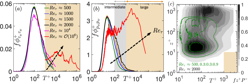
Figure 1: Premultiplied energy spectra of (a) ${\tau}_{w}$, (b) $p_{w}$ and (c) spectrogram of the bulk turbulence production (${z^{+}}{P^{+}}$) as a function of $T^{+}$. Data for 500 $\lesssim$ $Re_{\tau}$ $\lesssim$ 2000 is from Eitel-Amor et al. (2014), at $Re_{\tau}$ $\sim$ $\mathcal{O}$($10^{4}$) is from Marusic et al. (2021), and that at $Re_{\tau}$ $\sim$ $\mathcal{O}$($10^{6}$) is from the SLTEST data acquired by (a) Marusic & Heuer (2007) and (b) Klewicki et al. (2008). Grey and yellow coloured backgrounds in (a-c) indicate the intermediate ($\mathcal{O}$($10^{2}$) $\lesssim$ $T^{+}$ $\lesssim$ $\mathcal{O}$($10^{3}$) and large scale ranges ($T^{+}$ $\gtrsim$ $\mathcal{O}$($10^{3}$)), respectively.

The origin of the large-scale inertia-dominated energy in the outer region has now been well established in the literature (Lee & Moser, 2019), based on the turbulent kinetic energy (TKE) production term, $P^{+}$ = -2${{\overline{uw}}^{+}}({{\partial}{{\overline{U}}^{+}}}/{{\partial}{z^{+}}})$. Here, $u$, $v$ and $w$ represent instantaneous velocity fluctuations along the streamwise ($x$), spanwise ($y$) and wall-normal ($z$) directions respectively, while capital letters and overbar indicate time-averaging. Figure 1(c) shows the premultiplied spectra of the bulk turbulence production (${z^{+}}{P^{+}}$($z^{+}$; $T^{+}$)) from the same simulation data sets as in figures 1(a,b), confirming the absence of energy production at $T^{+}$ $>$ 1000 in the near-wall region ($z^{+}$ $<$ 10). While several past studies have quantified and predicted the large-scale signatures superimposed on ${\tau}_{w}$ (Metzger & Klewicki, 2001; Mathis et al., 2013; Vinuesa et al., 2015), fundamental understanding of the large-scale energy-transfer mechanisms, particularly the energy transport from the outer region towards the wall, is still lacking.

With regards to the differences between ${\tau}_{w}$ and $p_{w}$ in $\mathcal{O}$($10^{2}$) $\lesssim$ $T^{+}$ $\lesssim$ $\mathcal{O}$($10^{3}$), although TKE is produced in this scale range near the wall, the constant energy contours in figure 1(c) exhibit a convincing collapse for different $Re_{\tau}$. Hence, the $Re_{\tau}$-increase of $f{{\phi}^{+}_{{{p}_{w}}{{p}_{w}}}}$ in this intermediate-scale range is also owing to the energization of turbulence motions farther away from the wall, which, however, do not seem to influence $f{{\phi}^{+}_{{{\tau}_{w}}{{\tau}_{w}}}}$. This difference likely stems from the fact that $p_{w}$ is dependent on the velocity field across the entire boundary layer (via the pressure Poisson equation), which also includes motions physically detached from the wall. In contrast, ${\tau}_{w}$ is dictated by the near-wall velocity gradient, which is influenced solely by motions physically attached to the wall. Hence, obviously the $Re_{\tau}$ trend of $f{{\phi}^{+}_{{{p}_{w}}{{p}_{w}}}}$ is governed by a broader range of eddy types than those responsible for the behaviour of $f{{\phi}^{+}_{{{\tau}_{w}}{{\tau}_{w}}}}$. Any advancements in our fundamental understanding of these governing motions would be valuable for designing drag and noise reduction strategies at high $Re_{\tau}$.

1.1 The role of active and inactive components

The present study explores the ability of the attached-eddy framework (Townsend, 1976) to provide a phenomenological explanation for the questions raised above. This is motivated by the fact that the same framework has been previously successful in predicting the ${\tau}_{w}$- and $p_{w}$-spectra, associated with the inertial scales, across a broad $Re_{\tau}$-range (Marusic et al., 2021; Ahn et al., 2010). Per Townsend’s hypothesis, the outer region ($z$ $\gtrsim$ $z_{\rm min}$) of a high-$Re_{\tau}$ wall-bounded flow can be statistically represented by a hierarchy ($\mathcal{O}$($z_{\rm min}$) $\lesssim$ $\mathcal{H}$ $\lesssim$ $\mathcal{O}$($\delta$)) of geometrically self-similar, inviscid, wall-scaled eddies dominated by inertia, where $\mathcal{H}$ is the eddy height. These eddies have been classically referred to as attached eddies in the literature, in reference to their scaling with $z$ and $\overline{U}_{\tau}$, and not necessarily implying their physical extension to the wall. Townsend (1976) proposed that these wall-scaled eddies have a population density varying inversely to their height $\mathcal{H}$, leading to their cumulative velocity contributions at $z$ $\gtrsim$ $z_{\rm min}$ to follow (at asymptotically high $Re_{\tau}$):

$${{\overline{u^{2}}}^{+}} ={B_{1}}-{A_{1}}\;\ln({z}/{\delta}),$$ (1)

$${{\overline{v^{2}}}^{+}} ={B_{2}}-{A_{2}}\;\ln({z}/{\delta}),$$

$${{\overline{w^{2}}}^{+}} ={B_{3}}\;\text{and}$$

$${{\overline{uw}}^{+}} ={B_{4}},$$

where $B_{1-4}$ and $A_{1-2}$ are constants. The increased availability of high-$Re_{\tau}$ data over the past two decades have provided considerable empirical support to these expressions (see Deshpande et al., 2021 and references therein), which are however limited to the log-region of the TBL. The disagreement beyond the log region is owing to the statistical significance of the non-wall-scaled eddy-type motions coexisting in boundary layers, particularly in its wake region (Marusic & Perry, 1995). While the expressions for ${\overline{u^{2}}}^{+}$ and ${\overline{v^{2}}}^{+}$ in (1) suggest their dependence on $Re_{\tau}$, ${\overline{w^{2}}}^{+}$ and ${\overline{uw}}^{+}$ are postulated to be $Re_{\tau}$-independent. Townsend (1976) explained this by proposing that the flow at any point of observation ($z$ $\gtrsim$ $z_{\rm min}$) comprises of two components of wall-scaled eddies (figure 2) $-$ an ‘active’ component of wall-scaled eddy that is responsible for local turbulent transfer and accounts for the instantaneous Reynolds shear stresses ($uw$) at $z$, and an ‘inactive’ component that does not contribute to $uw$ at $z$. Here, the inactive component predominantly comes from wall-scaled eddies much taller than $z$, which contribute to $uw$ (i.e., behave as active motions) at wall-normal locations larger than $z$. Hence, while the active component is solely responsible for the local TKE production, Townsend (1976) described inactive motions as non-local ‘swirling motions’ whose “effect on that part of the layer between the point of observation and the wall is one of slow random variation of ‘mean velocity’ which cause corresponding variation of wall stress.” These statements were supported by Bradshaw (1967) and de Giovanetti et al. (2016), who hypothesized that the inactive parts of the wall-scaled eddies are responsible for transporting large-scale energy produced in the outer layer (by active parts), to the wall. As per Bradshaw (1967), this process was necessary to maintain the near-wall energy balance and is sketched in figures 2(c-e).

Although the non-local wall-normal transport of large-scale energy has been previously observed through spectral analysis of the TKE budget equations (Cho et al., 2018; Lee & Moser, 2019), its connection with the inactive part of the wall-scaled eddies has never been definitively established, primarily due to the lack of a reliable flow-decomposition methodology. Along the same lines, while the association of $p_{w}$-signatures with intense $uw$ events is well known (Gibeau & Ghaemi, 2021; Baars et al., 2024), their correlation with $uw$-contributing (active) and non-contributing (inactive) components has never been explicitly established. Recently, Deshpande et al. (2021) proposed a spectral linear stochastic estimation (SLSE)-based methodology that enables data-driven decomposition of the log-region motions into their corresponding active and inactive components. This provides an opportunity to confirm the association of active/inactive components with ${\tau}_{w}$ and $p_{w}$, and thereby explain their $Re_{\tau}$-variation based on the $Re_{\tau}$-growth of the wall-scaled eddy hierarchy (figure 2).

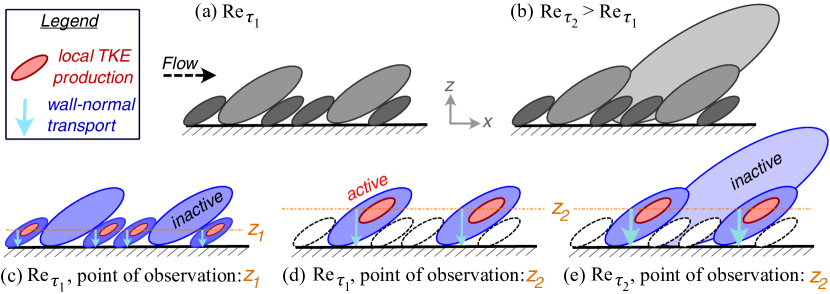
Figure 2: Conceptual sketches of wall-scaled eddies in a TBL at relatively (a) low ($Re_{{\tau}_{1}}$) and (b) high ($Re_{{\tau}_{2}}$) Reynolds numbers. (c-e) depict the roles of the active and inactive parts of wall-scaled eddies in the energy-transfer mechanisms per hypothesis of Bradshaw (1967) and de Giovanetti et al. (2016). Blue and red sections respectively correspond to the inactive and active parts of the wall-scaled eddies (grey-scaled), which are defined based on the point of observation, $z$: (c) $z_{1}$ or (d,e) $z_{2}$. In (d,e), white eddies with dashed contours are centred lower than $z$, and hence are not involved in either local TKE production at $z$ (red region), or non-local energy transport from $z$ to the wall (cyan arrows). Greater thickness of arrows in (e) indicates larger transport magnitude at higher $Re_{\tau}$.

The concept of active and inactive motions is associated with the spatial distribution of velocity signatures generated by the inviscid wall-scaled (attached) eddies (Deshpande et al., 2021), which are only restricted by the impermeability condition at the wall ($w$ $=$ 0 $\neq$ $u$, $v$ at $z$ $=$ 0). This boundary condition leads to spatially localized $w$-signatures, and consequently $uw$-signatures, at $z$ from any wall-scaled eddy of $\mathcal{H}$ $\sim$ $\mathcal{O}$($z$), while the $u$- and $v$-signatures extend across 0 $\lesssim$ $z$ $<$ $\mathcal{H}$ (i.e., non-local). Considering a flow field comprising purely wall-scaled eddies (figure 2), active contributions at $z$ are hence solely associated with eddies of height, $\mathcal{H}$ $\sim$ $\mathcal{O}$($z$), which contribute to $u$, $v$, $w$ and hence $uw$, at $z$. The inactive contributions are associated with relatively tall wall-scaled eddies: $\mathcal{O}$($z$) $\ll$ $\mathcal{H}$ $\lesssim$ $\mathcal{O}$($\delta$). These contribute to $u$($z$) and $v$($z$), but not $w$($z$) and $uw$($z$). This can be expressed as (Panton, 2007; Deshpande & Marusic, 2021):

$${u}(z) ={u_{a}}(z)+{u_{ia}}(z),$$ (2)

$${v}(z) ={v_{a}}(z)+{v_{ia}}(z)\;\text{and}$$

$${w}(z) ={w_{a}}(z),$$

where subscripts $a$ and $ia$ respectively denote active and inactive components. The variances can be decomposed following (Panton, 2007; Deshpande & Marusic, 2021):

$${{\overline{u^{2}}}^{+}} ={{\overline{u^{2}_{ia}}}^{+}}+{{\overline{u^{2}_{a}}}^{+}}+2\overline{{u_{ia}}{u_{a}}},$$ (3)

$${{\overline{v^{2}}}^{+}} ={{\overline{v^{2}_{ia}}}^{+}}+{{\overline{v^{2}_{a}}}^{+}}+2\overline{{v_{ia}}{v_{a}}},$$

$${{\overline{w^{2}}}^{+}} ={{\overline{w^{2}_{a}}}^{+}}\textrm{and}$$

$${{\overline{uw}}^{+}} ={{\overline{{u_{a}}{w}}}^{+}}+{{\overline{{u_{ia}}{w}}}^{+}}.$$

While $\overline{{u_{ia}}{u_{a}}}$, $\overline{{v_{ia}}{v_{a}}}$ and $\overline{{u_{ia}}{w}}$ = 0 for a traditionally conceptualized wall-scaled eddy field (i.e., considering only linear superposition of velocity fluctuations associated with various hierarchies of wall-scaled eddies), that is not true for an actual/real wall-bounded flow (Deshpande et al., 2021; Deshpande & Marusic, 2021). A real TBL also comprises very-large-scale inertial motions/superstructures which are inherently inactive per definition of Townsend (1976) and interact non-linearly with/modulate the eddies local to $z$ (Metzger & Klewicki, 2001; Mathis et al., 2013; Baars et al., 2016). The exact relationship between these non-linear interactions and the large scales, however, is a topic of ongoing debate (Andreolli et al., 2023). This, combined with the fact that the magnitude of these non-linear interactions are smaller than individual $\overline{u^{2}_{ia}}$ and $\overline{u^{2}_{a}}$ components (3; Deshpande & Marusic, 2021), makes their investigation beyond the scope of this study. The present study aims to deploy the decomposition methodology facilitating (2) on instantaneous flow fields of published data sets to analyze the active and inactive contributions to ${\tau}_{w}$ and $p_{w}$. The work builds over the past successes of the decomposition methodology (Deshpande et al., 2021; Deshpande & Marusic, 2021) that has yielded empirical support for several characteristics of active and inactive components hypothesized previously. This includes the $z$-scaling behaviour of ${{\overline{uw}}^{+}}$ $\approx$ ${\overline{{u_{a}}{w}}}^{+}$ and ${{\overline{u^{2}_{a}}}^{+}}$, and the inverse logarithmic variation of ${{\overline{u^{2}_{ia}}}^{+}}$ associated with the $k^{-1}$-scaling, to list a few.

2 Data sets and methodology

The present study considers two previously published multi-point data sets across a large $Re_{\tau}$ range: $\mathcal{O}$($10^{3}$) $\lesssim$ $Re_{\tau}$ $\lesssim$ $\mathcal{O}$($10^{6}$), for the SLSE analysis. The low-$Re_{\tau}$ data set is from the high-resolution large-eddy simulation (LES) of a zero-pressure-gradient (ZPG) TBL by Eitel-Amor et al. (2014), which was computed over a numerical domain large enough for the TBL to evolve up to $Re_{\tau}$ $\approx$ 2000. Here, we analyze the synchronously sampled time-series of the desired wall properties (${\tau}^{+}_{w}$, ${p}^{+}_{w}$), as well as the overlying flow field ($u^{+}$, $w^{+}$), at designated streamwise locations of the numerical domain corresponding to $Re_{\tau}$ $\approx$ 500, 1000, 1500 and 2000. The time series were sampled across the entire domain cross-section ($y-z$), with a resolution of ${\Delta}t^{+}$ $\lesssim$ 0.5 and for a total eddy-turnover time (${t_{\rm samp}}{U_{\infty}}/{\delta}$) $\approx$ 243, where $U_{\infty}$ is the freestream speed. Combined with the option to ensemble-average across the span, these time-series are sufficient to obtain a sufficiently converged frequency spectra for capturing the inertial phenomena (demonstrated in Eitel-Amor et al., 2014).

The high-$Re_{\tau}$ ($\sim$ $\mathcal{O}$($10^{6}$)) data set is from the neutrally-buoyant surface layer at the SLTEST facility in Utah (Marusic & Heuer, 2007). The data comprises synchronously acquired time-series of ($u^{+}$, $w^{+}$) from five sonic anemometers positioned on a vertical tower, within the log region (0.0025 $<$ $z/{\delta}$ $<$ 0.0293), and wall-shear stress-signals (${\tau}^{+}_{w}$) measured using a custom-designed sensor placed vertically below the sonics. This data was acquired at a time resolution of ${\Delta}t^{+}$ $\lesssim$ 78.4 and for a total of 175 eddy-turnover times, across a viscous-scaled measuring volume of 1400 (of sonics).

While the sampling intervals for both LES and SLTEST data sets are not sufficient for fully converging/resolving the very-large-scale phenomena (quantitatively), they have been analyzed previously by Deshpande et al. (2024) and found to be sufficient to attain an accurate qualitative understanding. This was demonstrated by repeating the same statistical analysis (as presented ahead in §2.1) on the simultaneous ($u^{+}$,$w^{+}$) and ${\tau}^{+}_{w}$ measurements conducted in the large Melbourne wind tunnel (Deshpande & Marusic, 2021), time series for which were sampled for a much longer time interval and at greater frequency. The results and trends derived from the wind-tunnel data were qualitatively consistent with those obtained from the LES and SLTEST data sets, which will serve as the basis for the present study. Both these data sets provide rare access to velocity-fluctuation time series across the log-region synchronously with ${\tau}_{w}$, for TBLs spanning a broad $Re_{\tau}$ range ($10^{3}$–$10^{6}$). This offers a unique opportunity to directly test the hypothesis of Bradshaw (1967) and de Giovanetti et al. (2016), regarding TKE production and transport mechanisms from log region to the wall, and understand how they affect ${\tau}_{w}$ and $p_{w}$. Our present conclusions will only depend on the qualitative energy variation across $z$, and not focus on its quantification/scaling (requiring convergence). We note that although the SLTEST flows are transitionally rough TBLs, the roughness effects are insignificant beyond the roughness sublayer (Klewicki et al., 2008; Marusic & Heuer, 2007). Hence, the roughness will not influence inertial eddies, which are our primary focus.

2.1 Data-driven flow-decomposition methodology

The multi-point nature of both LES and SLTEST data sets permit theoretical estimation of $u_{a}$ and $u_{ia}$ by following the SLSE-based methodology proposed previously in Deshpande et al. (2021) and Deshpande & Marusic (2021). Throughout this paper, we limit our SLSE analysis to the log region where the concept of active and inactive motions, as well as expressions in (1), have received considerable empirical support (Deshpande et al., 2021). Per the SLSE methodology (Baars et al., 2016), the instantaneous component $u_{ia}$($z$) in the log region can be obtained by:

$${\widetilde{u_{ia}}}(z^{+};{T^{+}})={{H_{L}}(z^{+};{T^{+}})}{\widetilde{u_{\tau}}}({T^{+}}).$$ (4)

Here, ${\widetilde{u_{\tau}}}$($T^{+}$) = $\sqrt{{\widetilde{{\tau}_{w}}}/{\rho}}$ = $\mathcal{F}$($u_{\tau}$($t^{+}$)) is essentially the Fourier transform of the friction velocity fluctuations, $u_{\tau}$($t^{+}$) in time $t$, where $\rho$ is density. ${\widetilde{u_{\tau}}}$ acts as the scale-specific unconditional input required to obtain the scale-specific conditional output, ${\widetilde{u_{ia}}}(z^{+};{T^{+}})$. Further, $H_{L}$ is the complex-valued linear transfer kernel reconstructed by cross-correlating the synchronously acquired $\widetilde{u}$($z^{+}$) and $\widetilde{u_{\tau}}$ following:

$${H_{L}}(z^{+};{T^{+}})=\frac{\{\widetilde{u}(z^{+};{T^{+}}){{\widetilde{u_{\tau}}}^{\ast}}({T^{+}})\}}{\{{{\widetilde{u_{\tau}}}({T^{+}})}{{\widetilde{u_{\tau}}}^{\ast}}({T^{+}})\}},$$ (5)

where the curly brackets ($\{\}$) and asterisk ($\ast$) denote ensemble averaging and complex conjugate, respectively. Here, the definition of $H_{L}$ in (5) is underpinned by the description presented in $\S$1 that the inactive components at $z^{+}$ influence $u_{\tau}$, making $\widetilde{u_{ia}}$ essentially a subset of the total momentum $\widetilde{u}$ that is coherent with $\widetilde{u_{\tau}}$. Figures 3(a,b) depict $|H_{L}|$(${z^{+}}$, $T^{+}$) computed from the LES and SLTEST data sets at $z^{+}$ within the log region, alongside the premultiplied spectra of $u_{\tau}$ (${f}{{\phi}^{+}_{{u_{\tau}}{u_{\tau}}}}$), where $||$ represents the modulus. Before plotting, $|H_{L}|$ has been smoothed based on a 25% bandwidth moving filter (BMF; Baars et al., 2016). This is done to remove noise emerging from the mathematical operations in (5), which are conducted on a per-scale basis. The trends observed in $|H_{L}|$, as depicted in figure 3, align with similar statistics computed using long time-series signals from the Melbourne wind-tunnel data set (Deshpande & Marusic, 2021; Deshpande et al., 2024), reaffirming their physical nature rather than being artefacts of insufficient convergence.

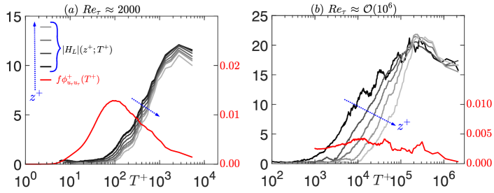
Figure 3: Absolute values of the linear transfer kernel ($|H_{L}|$($z^{+}$;$T^{+}$); equation 5) computed for the (a) LES and (b) SLTEST data and plotted in different shades of grey. Here, $|H_{L}|$ is plotted for $z^{+}$ limited to the log region and its ordinate is considered on the primary vertical axis (left; in black). While, the solid red line represents the premultiplied spectra of the friction velocity ($f{{\phi}^{+}_{{u_{\tau}}{u_{\tau}}}}$) and its ordinate is considered on the secondary vertical axis (right; in red).

Significantly, for both the LES and SLTEST data, $|H_{L}|$ extends to sufficiently large $T^{+}$ values where the corresponding $f{{\phi}^{+}_{{u_{\tau}}{u_{\tau}}}}$ is negligible beyond the considered range. This ensures proper estimation of the very-large-scale ${\widetilde{u_{ia}}}$ signal. Similarly, the time resolution and frequency response of the wall-shear-stress sensor at high $Re_{\tau}$, despite limiting the measurement of wall-shear-stress spectrum to $T^{+}$ $\gtrsim$ 1000 (figures 1a, 3b), is sufficient to resolve ${\widetilde{u_{ia}}}$ considering $|H_{L}|$ $\sim$ 0 at $T^{+}$ $\lesssim$ 1000. Once ${\widetilde{u_{ia}}}$ is obtained, its time-domain equivalent can be calculated simply by taking the inverse Fourier transform (Deshpande & Marusic, 2021): ${{{u}_{ia}}(z^{+};{t^{+}})}$ = ${\mathcal{F}^{-1}}({{\widetilde{{u}_{ia}}}(z^{+};{T^{+}})})$. Considering the discussion on the past hypotheses in $\S$1.1, the novel analysis here is not to establish the correlation of $u_{ia}$ with ${\tau}_{w}$ (which is imposed by definition in equation 4), but to investigate the variation of simultaneously acquired $u_{ia}$-signals across various $z$-locations in the log region. Estimation of $u_{ia}$ also permits calculation of the $u_{a}$-time series by simple subtraction, ${{{u}_{a}}(z^{+};{t^{+}})}$ = ${{{u}}(z^{+};{t^{+}})}$ – ${{{u}_{ia}}(z^{+};{t^{+}})}$. This enables computation of the Reynolds shear stresses associated with the active motions: ${u_{a}}w$($z^{+}$; $t^{+}$), which should correspond with the net Reynolds shear stresses ($uw$($z^{+}$; $t^{+}$)) per Townsend’s (1961) hypothesis. These hypotheses will be tested in this study using simultaneously acquired time series signals across the log region.

3 Results and discussions

3.1 Active and inactive contributions to the wall-shear stress

This section focuses on responding to research question (i) raised in $\S$1, regarding the role played by inactive motions in transporting large-scale energy from the outer region to the wall (to explain ${\tau}_{w}$-signatures at large $T^{+}$). Figures 4(a,f) plot a small subset of the full $u^{+}$-time series sampled in the log region, synchronously with that of ${\tau}^{+}_{w}$, from the LES and SLTEST data sets respectively. This data is used to obtain the corresponding active (figures 4c,h) and inactive components (figures 4e,j) of $u^{+}$ by following the procedure described in $\S$2.1. Also plotted in figures 4(b,g) are the $w^{+}$-signals corresponding to the same instants as those considered for the $u^{+}$-signals.

As expected based on (4), $u_{ia}$-signals correspond predominantly to low-frequency features (i.e., large $T^{+}$) that are highly correlated with ${\tau}_{w}$, while $u_{a}$-signals are representative of the relatively high-frequency phenomena that are uncorrelated with ${\tau}_{w}$. Notably, the $w$-signals exhibit same characteristics as those of $u_{a}$ across the log region. This is consistent with Townsend’s description of $u_{a}$ and $w$ being associated with wall-scaled eddies local to $z$ (i.e., $\mathcal{H}$ $\sim$ $z$), while $u_{ia}$ corresponds to relatively taller and larger wall-scaled eddies ($\mathcal{O}$($z$) $\ll$ $\mathcal{H}$ $\lesssim$ $\mathcal{O}$($\delta$)) with contributions extending to the wall (see figure 2 and equation 2). Townsend’s (1976) hypothesis is mainly centred on the fact that the active components are solely responsible for the shear stresses and TKE production across log region $-$ this is clearly evident from figures 4(d,i) comparing ${u_{a}}w$ (in red) with $uw$ (in thicker black lines). The good overlap of the two signals, across $10^{3}$ $\lesssim$ $Re_{\tau}$ $\lesssim$ $10^{6}$, is a testament to the capability of the SLSE-based methodology of extracting the active components. While the success of this data-decomposition methodology has also been demonstrated previously using the Melbourne wind-tunnel data set at $Re_{\tau}$ $\sim$ $10^{4}$ (based on statistically independent time-series signals across $z$; Deshpande & Marusic, 2021), this work showcases it for simultaneously acquired signals across the log region for the first time.

Interestingly, there are certain portions of the time series in figures 4(d,i) where ${u_{a}}w$ does not exactly replicate $uw$ (indicated by green background). These portions are representative of the non-linear interactions between active motions and the inactive superstructures (i.e., ${u_{ia}}w$). They become non-negligible (in an instantaneous sense) only at time instants corresponding to high-amplitude signatures in $u_{ia}$, which are also highlighted by green background shading in figures 4(e,j). Notably, these $u_{ia}$-signals exhibit a discernible increase in fluctuation magnitudes as $z/{\delta}$ decreases within the log region, which can be compared based on the dashed grey lines in figures 4(e,j) representing zero magnitude (for signals at each $z$ location). This suggests a wall-ward transport of streamwise momentum by the inactive components (indicated by the dashed black arrows) that is locally produced at each $z$ by the active component (conceptualized in figures 2c-e). Since the correlation between $u_{ia}$ and ${\tau}_{w}$ has already been quantified by $|H_{L}|$ via (5), we know that this transport occurs all the way down to the wall. The novel result here is the time-synchronized increment in $u_{ia}$ magnitude with reducing $z$, which is an outcome of the flow decomposition. It presents a direct evidence of the non-local transfer of momentum/energy in the wall-normal direction across a broad $Re_{\tau}$-range, which was previously noted only via spectral distributions at low $Re_{\tau}$ (Cho et al., 2018; Lee & Moser, 2019).

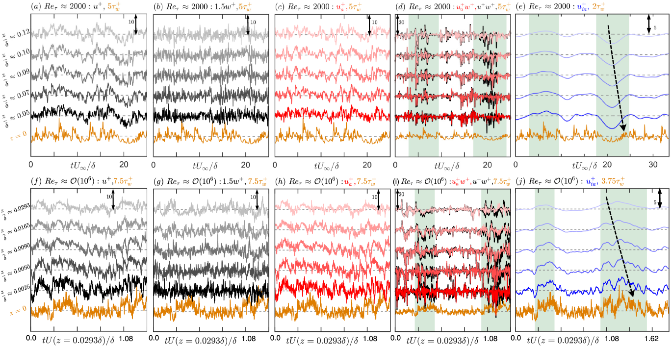
Figure 4: Instantaneous (a,f) streamwise and (b,g) amplified wall-normal velocity fluctuations (in black) at various $z^{+}$ decomposed into their corresponding (c,h) active ($u^{+}_{a}$; in red) and (e,j) inactive ($u^{+}_{ia}$; in blue) components via the SLSE-based methodology discussed in $\S$2. Note the different vertical offsets for various time series as well as different ordinate ranges. (d,i) compares the time series of the full momentum flux (${u^{+}}{w^{+}}$; in black) and that associated with the active motions (${u^{+}_{a}}{w^{+}}$; in red). Dark to light shading indicates increase in $z/{\delta}$ across all plots. The synchronously acquired time series of the wall-shear-stress fluctuations (${\tau}^{+}_{w}$; in golden) have been plotted for: (a-e) $Re_{\tau}$ $\approx$ 2000 (LES) and (f-j) $Re_{\tau}$ $\approx$ $\mathcal{O}$($10^{6}$) (SLTEST) data sets and has been intentionally amplified for clarity. Background green shading in (d,e,i,j) highlights portions of time series associated with relatively high magnitudes of $u^{+}_{ia}$, which increase with decreasing $z/{\delta}$ indicating downward momentum transfer.

The significance of this empirical evidence is highlighted by quoting text directly from de Giovanetti et al. (2016), who hypothesized that: “the energy-containing motions, which essentially reside in the logarithmic and outer regions, transport the streamwise momentum to the near-wall region through their inactive part, while generating Reynolds shear stress with their wall-detached wall-normal velocity component in the region much further from the wall”. Here, de Giovanetti et al. (2016) use ‘wall-detached’ to essentially refer to the active component responsible for the $w$-fluctuations, given that it does not physically extend down to the wall. Hence, figures 4(d,e,i,j) cumulatively provide strong empirical evidence in support of the hypothesis proposed by Bradshaw (1967) and de Giovanetti et al. (2016).

The present analysis also demonstrates the unique capability to segregate instantaneous flow components associated with two key energy-transfer mechanisms in high $Re_{\tau}$ wall flows $-$ TKE production and its wall-normal transport. This is a promising development for design of real-time control strategies targeting either of these mechanisms. However, more work would be required with respect to identifying 3-D flow features/motions responsible for these mechanisms, before such strategies can be actualized. As is evident from figures 4(b,g), the wall-normal transport cannot be explained purely based on the $w$-time series sampled across limited (and large) wall-normal offsets. But it could be possible by analyzing velocity fluctuations/gradients acquired with good wall-normal resolution, which is however beyond the scope of the present study.

Although not depicted here explicitly, we note for completeness that the active contributions computed for both LES and SLTEST data exhibit characteristics similar to those expected based on Townsend’s (1976) hypothesis, with $\overline{u^{2}_{a}}$ $\approx$ constant in the log region (Deshpande et al., 2021; Deshpande & Marusic, 2021). The data considered in this study does not permit a meaningful direct comparison of $\overline{u^{2}_{ia}}$ with $\overline{{\tau}^{2}_{w}}$ for increasing $Re_{\tau}$, owing to mismatched $z^{+}$ and $z/{\delta}$ for the two data sets, alongside the under-resolved measurement of $\tau_{w}$ (both spatially and temporally). Interested readers may refer to discussions and analyses presented in Deshpande et al. (2021), wherein it is suggested that the $\overline{u^{2}_{ia}}$ at a fixed $z/{\delta}$ would be expected to increase with $Re_{\tau}$ due to the broadening of the wall-scaled eddy hierarchy (see figures 2b,e). This insight potentially explains the Reynolds-number dependency of large-scale signatures in the ${\tau}_{w}$-spectra, as noted in figure 1(a) and discussed in the literature (Örlü & Schlatter, 2011; Mathis et al., 2013).

3.2 Active and inactive contributions to the wall-pressure

This section focuses on addressing the research question (ii) raised in $\S$1, regarding the inertial motions responsible for the $Re_{\tau}$-growth of the $p_{w}$-spectra. For this, we compute the linear coherence spectrum (Gibeau & Ghaemi, 2021; Baars et al., 2024) between the fluctuating wall-pressure and velocity fluctuations following:

$${{\gamma}^{2}_{{u_{i}}{p_{w}}}}(z^{+};{T^{+}})=\frac{|\{\widetilde{u_{i}}(z^{+};{T^{+}}){{\widetilde{p_{w}}}^{\ast}}({T^{+}})\}|^{2}}{{\{{{\widetilde{u_{i}}}({z^{+};T^{+}})}{{\widetilde{u_{i}}^{\ast}}(z^{+};{T^{+}})\}}}{\{{{\widetilde{p_{w}}}(T^{+})}{{\widetilde{p_{w}}^{\ast}}({T^{+}})\}}}},$$ (6)

where $u_{i}$ can be either $u$, $w$, $u_{ia}$ or $u_{a}$, (||) represents absolute values, while all other notations are the same as in (5). Note that ${\gamma^{2}_{{u_{i}}{p_{w}}}}$ can be interpreted as the spectral equivalent of a physical two-point correlation between $p_{w}$ and $u_{i}$, which varies between 0 $\leq$ ${\gamma^{2}_{{u_{i}}{p_{w}}}}$ $\leq$ 1 by definition. Furthermore, ${\gamma^{2}_{{u}{p_{w}}}}$ and ${\gamma^{2}_{{w}{p_{w}}}}$ have been analyzed previously for a canonical TBL at $Re_{\tau}$ $\approx$ 2000 by Gibeau & Ghaemi (2021), to establish the scale-based coupling between the inertial motions and the large-scale pressure (LSP; 0.8 $<$ $T{U_{\infty}}/{\delta}$ $<$ 7), as well as the very-large-scale pressure (VLSP; $T{U_{\infty}}/{\delta}$ $>$ 7) regions of the $p_{w}$-spectrum. To validate our analysis, we recompute ${\gamma^{2}_{{u}{p_{w}}}}$ and ${\gamma^{2}_{{w}{p_{w}}}}$ (figures 5a,b) from the LES data set at $Re_{\tau}$ $\approx$ 2000 and compare it with the outer-scaled $p_{w}$-spectrum (figure 5c). The coherence spectra depicts characteristics consistent with those reported by Gibeau & Ghaemi (2021): the VLSP region is associated with relatively strong coherence between $u$ and $p_{w}$, but not between $w$ and $p_{w}$. While in case of LSP, reasonable coherence can be noted between both $u$-$p_{w}$ and $w$-$p_{w}$. If the same spectrograms were plotted as a function of streamwise wavelengths based on Taylor’s hypothesis (i.e., ${\lambda}^{+}_{x}$ $=$ 2${\pi}{T^{+}}{{\overline{U}}^{+}}$($z^{+}$)), the energetic ridges of ${\gamma^{2}_{{u}{p_{w}}}}$ and ${\gamma^{2}_{{w}{p_{w}}}}$ would respectively exhibit distance-from-the-wall scalings: ${{\lambda}_{x}}/z$ = 14 and ${{\lambda}_{x}}/z$ = 8.5 (not shown here), consistent with Baars et al. (2024). This confirms the association of the $p_{w}$-spectrum with the wall-scaled eddy hierarchy coexisting in the inertial/large-scale range.

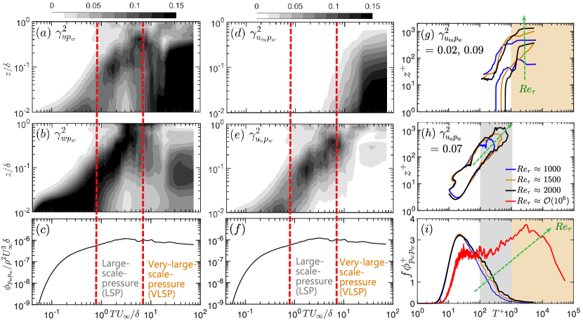
Figure 5: Linear coherence spectrum (${\gamma}^{2}_{{u_{i}}{p_{w}}}$; equation 6) computed between $u_{i}$($z^{+}$) and $p_{w}$ as a function of outer- or inner-scaled $T$: (a) ${\gamma}^{2}_{{u}{p_{w}}}$, (b) ${\gamma}^{2}_{{w}{p_{w}}}$, (d,g) ${\gamma}^{2}_{{u_{ia}}{p_{w}}}$ and (e,h) ${\gamma}^{2}_{{u_{a}}{p_{w}}}$. (a,b,d,e) depict ${\gamma}^{2}_{{u_{i}}{p_{w}}}$ computed from $Re_{\tau}$ $\approx$ 2000 LES data and compared against the (c,f) outer-scaled $p_{w}$-spectrum plotted versus outer-scaled $T$. (g,h) respectively depict ${\gamma}^{2}_{{u_{ia}}{p_{w}}}$ and ${\gamma}^{2}_{{u_{a}}{p_{w}}}$ contours for data across various $Re_{\tau}$, which are compared against (i) $f{{\phi}^{+}_{{p_{w}}{p_{w}}}}$ plotted versus $T^{+}$.

Connecting the differences between ${{\gamma}^{2}_{{u}{p_{w}}}}$ and ${{\gamma}^{2}_{{w}{p_{w}}}}$ with the characteristics of active and inactive components discussed in $\S$1.1, it can be hypothesized that the $p_{w}$-spectrum in the LSP and VLSP ranges, is respectively, correlated to the active and inactive motions. The availability of decomposed $u_{a}$ and $u_{ia}$ components, for the same data as in figures 5(a,b), permits us to directly test this hypothesis by analyzing ${{\gamma}^{2}_{{u_{ia}}{p_{w}}}}$ and ${{\gamma}^{2}_{{u_{a}}{p_{w}}}}$ depicted in figures 5(d,e), respectively. It is evident that the coherence between $u_{ia}$-$p_{w}$ is limited to the VLSP range, while that between $u_{a}$-$p_{w}$ is predominantly in the LSP range, similar to ${{\gamma}^{2}_{{w}{p_{w}}}}$. All the observations are consistent with our hypothesis above, with the similarity between ${{\gamma}^{2}_{{w}{p_{w}}}}$ and ${{\gamma}^{2}_{{u_{a}}{p_{w}}}}$ expected considering $w$-signatures are predominantly active contributions (see equation 2). The present results offer phenomenological explanations for the conclusions drawn by Gibeau & Ghaemi (2021), who associated $p_{w}$-fluctuations in the LSP range with Reynolds shear stress-carrying ejection and sweep events in the log region, i.e., the active components of the wall-scaled eddies. Conversely, $p_{w}$-fluctuations in the VLSP range were linked to large $\delta$-scaled motions and superstructures, which correspond with the inactive/non-local components discussed by Deshpande et al. (2021).

Since the wall-scaled eddy hierarchy grows by coexisting in a physically taller log region with increasing $Re_{\tau}$ (figures 2b,e; Deshpande et al., 2021), the association of the LSP and VLSP ranges, with $u_{a}$ and $u_{ia}$, can be used to explain the $Re_{\tau}$-variation of the $p_{w}$-spectrum. To this end, figures 5(g,h) respectively plot the constant energy contours of ${{\gamma}^{2}_{{u_{ia}}{p_{w}}}}$ and ${{\gamma}^{2}_{{u_{a}}{p_{w}}}}$ versus $T^{+}$ for 1000 $\lesssim$ $Re_{\tau}$ $\lesssim$ 2000, each of which exhibit their unique $Re_{\tau}$-trends. Notably, the contours of ${{\gamma}^{2}_{{u_{a}}{p_{w}}}}$ can be seen to grow and widen across a larger $T^{+}$ range with $Re_{\tau}$ (indicated by green arrows), which explains the $Re_{\tau}$-growth of the $p_{w}$-spectrum in the intermediate-scale range: $\mathcal{O}$($10^{2}$) $\lesssim$ $T^{+}$ $\lesssim$ $\mathcal{O}$($10^{3}$). It suggests that a physically taller log region comprises a broader hierarchy of $z$-scaled active components, which subsequently increases contributions to the $p_{w}$-spectrum. This is analogous to the broadening of the $\overline{uw}$-plateau ($\sim$ –1) in the log region with increasing $Re_{\tau}$ (Marusic & Perry, 1995). In contrast, the active motions do not contribute to the ${\tau}_{w}$-spectrum since they do not physically extend down to the wall, and consequently do not influence the near-wall velocity gradient (de Giovanetti et al., 2016). The contours of ${{\gamma}^{2}_{{u_{ia}}{p_{w}}}}$ can be seen extending across a larger $z$-range with $Re_{\tau}$, which is predominantly associated with the energization and increasing wall-normal extent of the large wall-scaled eddies and superstructures in viscous units (Mathis et al., 2013; Lee & Moser, 2019). At very high $Re_{\tau}$ $\sim$ $\mathcal{O}$($10^{6}$), these energetic superstructures along with a broad hierarchy of wall-scaled eddies (figure 2e) would contribute to the significantly enhanced VLSP signatures of the $p_{w}$-spectrum through their inactive component (figure 5i). The present analysis, hence, encourages detailed multi-point measurements and high-fidelity simulations in the future, that can quantify the pressure-velocity coupling at high-$Re_{\tau}$ ($\gtrsim$ $10^{4}$), with particular focus on structures in the log region.

4 Concluding remarks

This study explains the $Re_{\tau}$-dependent, large-scale contributions to the ${\tau}_{w}$- and $p_{w}$-spectra by invoking the attached- (wall-scaled) eddy framework (Townsend, 1976), based on active and inactive motions. Unique multi-point data sets are analyzed using an energy decomposition methodology to reveal the contributions from TKE-producing (active) and non-producing (inactive) components, at any wall-normal position in the log-region, to the ${\tau}_{w}$- and $p_{w}$-spectra. Inactive components of wall-scaled eddies are found to be responsible for the non-local wall-normal transport of the large-scale inertia-dominated energy, from its origin in the log region (i.e, produced by active components), to the wall. The result provides strong empirical evidence for the hypothesis proposed by Bradshaw (1967) and de Giovanetti et al. (2016). This explains the appearance of large-scale signatures in the ${\tau}_{w}$-spectra, even though no large-scale TKE production occurs in the near-wall region. In terms of their contribution to wall pressure, active and inactive components are respectively correlated with the intermediate and large-scale portions of the $p_{w}$-spectrum. Both components exhibit growth with increasing $Re_{\tau}$, which is attributed to the broadening of the wall-scaled eddy hierarchy.

While this study demonstrates the new found capability to extract the active and inactive components, while also shedding light on their role in the large-scale energy transfer mechanisms, it does not delve into the non-linear interactions between these motions. These interactions, which have been previously discussed in the literature to a certain extent (Cho et al., 2018; Lee & Moser, 2019), can likely explain the transfer of TKE produced by active components to the inactive component of the wall-scaled eddies, before it is transported downward to the wall (see figure 2). Nevertheless, the new phenomenological explanations provided in this study have the potential to inspire future real-time control strategies aimed at achieving energy-efficient drag and flow-noise reduction.

This work also suggests an increased dynamical significance of ‘sweeps’, i.e., the fourth quadrant (Q4) of the Reynolds shear stresses ($u$ $>$ 0, $w$ $<$ 0), which likely govern the wall-ward transport of streamwise momentum in high-$Re_{\tau}$ TBLs. While the growing statistical dominance of log region sweeps with $Re_{\tau}$ has been quantified via high-$Re_{\tau}$ experiments (Deshpande et al., 2021), more detailed work is required to demonstrate their role in the energy-transfer mechanisms of the TBL outer region.

Declaration of Interests

The authors report no conflict of interest.

References

- Ahn et al. (2010) Ahn, B.-K., Graham, W. R. & Rizzi, S. A. 2010 A structure-based model for turbulent-boundary-layer wall pressures. J. Fluid Mech. 650, 443–478.
- Andreolli et al. (2023) Andreolli, A., Gatti, D., Vinuesa, R., Örlü, R. & Schlatter, P. 2023 Separating large-scale superposition and modulation in turbulent channels. J. Fluid Mech. 958, A37.
- Baars et al. (2024) Baars, W. J., Dacome, G. & Lee, M. 2024 Reynolds-number scaling of wall-pressure–velocity correlations in wall-bounded turbulence. J. Fluid Mech. 981, A15.
- Baars et al. (2016) Baars, W. J., Hutchins, N. & Marusic, I. 2016 Spectral stochastic estimation of high-Reynolds-number wall-bounded turbulence for a refined inner-outer interaction model. Phys. Rev. Fluids 1 (5), 054406.
- Bradshaw (1967) Bradshaw, P. 1967 ‘Inactive’ motion and pressure fluctuations in turbulent boundary layers. J. Fluid Mech. 30 (2), 241–258.
- Cho et al. (2018) Cho, M., Hwang, Y. & Choi, H. 2018 Scale interactions and spectral energy transfer in turbulent channel flow. J. Fluid Mech. 854, 474–504.
- Deshpande & Marusic (2021) Deshpande, R. & Marusic, I. 2021 Characterising momentum flux events in high Reynolds number turbulent boundary layers. Fluids 6 (4), 168.
- Deshpande et al. (2021) Deshpande, R., Monty, J. P. & Marusic, I. 2021 Active and inactive components of the streamwise velocity in wall-bounded turbulence. J. Fluid Mech. 914, A5.
- Deshpande et al. (2024) Deshpande, R., Vinuesa, R. & Marusic, I. 2024 Characteristics of active and inactive motions in high-Reynolds-number turbulent boundary layers. Accepted in Proc. 13th Turbulence and Shear Flow Phenomenon (TSFP-13), Montréal, Canada arXiv:2404.18506 [physics.flu-dyn].
- Eitel-Amor et al. (2014) Eitel-Amor, G., Örlü, R. & Schlatter, P. 2014 Simulation and validation of a spatially evolving turbulent boundary layer up to Reθ= 8300. Int. J. Heat Fluid Flow 47, 57–69.
- Gibeau & Ghaemi (2021) Gibeau, B. & Ghaemi, S. 2021 Low-and mid-frequency wall-pressure sources in a turbulent boundary layer. J. Fluid Mech. 918, A18.
- de Giovanetti et al. (2016) de Giovanetti, M., Hwang, Y. & Choi, H. 2016 Skin-friction generation by attached eddies in turbulent channel flow. J. Fluid Mech. 808, 511–538.
- Klewicki et al. (2008) Klewicki, J. C., Priyadarshana, P. J. A. & Metzger, M. M. 2008 Statistical structure of the fluctuating wall pressure and its in-plane gradients at high Reynolds number. J. Fluid Mech. 609, 195–220.
- Lee & Moser (2019) Lee, M. & Moser, R. D. 2019 Spectral analysis of the budget equation in turbulent channel flows at high Reynolds number. J. Fluid Mech. 860, 886–938.
- Marusic et al. (2021) Marusic, I., Chandran, D., Rouhi, A., Fu, M. K., Wine, D. & others 2021 An energy-efficient pathway to turbulent drag reduction. Nat. Commun. 12 (1), 1–8.
- Marusic & Heuer (2007) Marusic, I. & Heuer, W. D. C. 2007 Reynolds number invariance of the structure inclination angle in wall turbulence. Phys. Rev. Lett. 99 (11), 114504.
- Marusic & Perry (1995) Marusic, I. & Perry, A. E. 1995 A wall-wake model for the turbulence structure of boundary layers. Part 2. Further experimental support. J. Fluid Mech. 298, 389–407.
- Mathis et al. (2013) Mathis, R., Marusic, I., Chernyshenko, S. I. & Hutchins, N. 2013 Estimating wall-shear-stress fluctuations given an outer region input. J. Fluid Mech. 715, 163–180.
- Metzger & Klewicki (2001) Metzger, M. M. & Klewicki, J. C. 2001 A comparative study of near-wall turbulence in high and low Reynolds number boundary layers. Phys. Fluids 13 (3), 692–701.
- Örlü & Schlatter (2011) Örlü, R. & Schlatter, P. 2011 On the fluctuating wall-shear stress in zero pressure-gradient turbulent boundary layer flows. Phys. Fluids 23 (2), 021704.
- Panton (2007) Panton, R. L. 2007 Composite asymptotic expansions and scaling wall turbulence. Philosophical Transactions of the Royal Society A: Mathematical, Physical and Engineering Sciences 365 (1852), 733–754.
- Townsend (1976) Townsend, A.A. 1976 The structure of turbulent shear flow, 2nd edn. CUP.
- Townsend (1961) Townsend, A. A. 1961 Equilibrium layers and wall turbulence. J. Fluid Mech. 11 (1), 97–120.
- Tsuji et al. (2007) Tsuji, Y., Fransson, J., Alfredsson, P. & Johansson, A. 2007 Pressure statistics and their scaling in high-Reynolds-number turbulent boundary layers. J. Fluid Mech. 585, 1–40.
- Vinuesa et al. (2015) Vinuesa, R., Hites, M. H., Wark, C. E. & Nagib, H. M. 2015 Documentation of the role of large-scale structures in the bursting process in turbulent boundary layers. Phys. Fluids 27 (10).