Construction and Accuracy of Electronic Continuum Models of Incommensurate Bilayer 2D Materials
Abstract.
Single-particle continuum models such as the popular Bistritzer-MacDonald model have become powerful tools for predicting electronic phenomena of incommensurate 2D materials and the development of many-body models aimed to model unconventional superconductivity and correlated insulators. In this work, we introduce a procedure to construct continuum models of arbitrary accuracy relative to tight-binding models for moiré incommensurate bilayers. This is done by recognizing the continuum model as arising from Taylor expansions of a high accuracy momentum space approximation of the tight-binding model. We apply our procedure in full detail to two models of twisted bilayer graphene and demonstrate both admit the Bistritzer-MacDonald model as the leading order continuum model, while higher order expansions reveal qualitative spectral differences.
1. Introduction
Research in incommensurate 2D multi-layered materials has grown rapidly since the discovery of unconventional superconductivity in twisted bilayer graphene (TBG) [9], which arise from many-body electron correlations. TBG along with other incommensurate layered materials with large moiré patterns have been investigated experimentally for many-body correlation effects [14, 24]. To understand these models, there is a strong push to construct many-body models [5, 19, 13]. The procedure involves finding a moiré-scale single-particle basis, and using this basis to construct a many-body basis and corresponding Hamiltonian. As such, a careful understanding of the single-particle basis is fundamental. Continuum models such as the popular Bistritzer-MacDonald (BM) model [6] have been a method of choice for TBG, and there have been efforts to construct similar models for other materials including layered transition metal dichalcogonides and incommensurate trilayer systems [10, 18]. These models allow one to have a band structure, where the system can be described by eigenvalues (or energies) as functions of momenta,
for momenta in a small moiré Brillouin zone, an eigenvalue index, moiré periodic eigenfunctions, and bands indexed by . In this work we will consider a moiré periodic continuum operator of the form
| (1.1) |
where is a linear self-adjoint matrix-valued function with eigenvalues tending to infinity in . We define to be matrix-valued and is a bounded operator on . This class of continuum models includes models such as the BM model. In the case of the BM model for TBG, is linear and the eigenvalues of grow linearly with . This representation allows one to observe effective band gaps and flat bands. TBG exhibits two overlapping almost flat bands in single-particle models near the Fermi energy [6], conditions implying the importance of many-body correlations. TBG’s almost flat bands become exactly flat in an approximation of the BM model known as the chiral model [20, 23, 2, 3, 4]. The spectral accuracy required in typical moiré applications scales inversely proportional to moiré length scale, making high accuracy critical. Significant progress has been made in quantifying the accuracy of the BM model of TBG. In [22], accuracy of the BM model relative to a simplified tight-binding model of TBG is quantified via analysis of spectrally localized wavepackets, and in [7, 8] the BM model is derived as an approximation of a DFT-informed incommensurate linear Schrödinger model by making use of a semiclassical expansion, and accuracy is quantified for the density of states.
The purpose of this work is to introduce a procedure to construct and quantify the accuracy of continuum models arising as approximations of tight-binding models. We quantify accuracy via accuracy of the density of states, but the procedure is extendable to other observables such as conductivity, local density of states, and momentum local density of states. As ab initio Wannierized tight-binding models are considered accurate for incommensurate 2D materials due to their Van der Waals interlayer interactions [11], this work provides a route for the construction of arbitrary order accuracy ab initio continuum models. For clarity of presentation, we focus on one orbital per atom TBG models, and illustrate our approach for two specific TBG models: a Wannierized physics model [11], and a simplified TBG model in [22]. We derive a family of continuum models indexed by orders of accuracy. The technique is to exploit an in-between highly accurate approximate model, the truncated momentum space model [17]. If we consider (1.1), we can change bases using Bloch theory to obtain the infinite matrix
| (1.2) |
where represents the moiré dual lattice and hopping functions
The momentum space model exhibits the same structure, but with modified hopping functions. We then realize via this Fourier representation continuum models as approximations of momentum space models via careful handling of matrix truncations and hopping function Taylor expansions with respect to about the Dirac points. The truncated momentum space models are known to exhibit exponential convergence in band structure and on observables. We find three critical truncation parameters determine accuracy of the continuum model corresponding to intralayer Taylor expansion order, interlayer expansion order, and hopping truncation. We prove and numerically verify the convergence rates. We anticipate this procedure to have applications in deriving continuum model for materials that have a well-converged momentum space model including more complex materials such as TMDCs, mechanically relaxed moiré systems [16], and multi-layers with two incommensurate periodicities. We do a case study of two models of TBG to illustrate the importance of accuracy control. We show that while both models of TBG have a leading order continuum model approximation of the BM model, the band structure for the two models in momentum space have significant differences near the flat band, which can be corrected by using a higher order continuum model. The profile when mechanical relaxation effects are included deviate from the BM model even more radically [16, 15].
The rest of this paper is organized as follows. In Section 2, we introduce the momentum space formulation and review previous momentum space results we need. In Section 3, we derive continuum models as approximations of tight-binding models. In Section 4, we analyze the convergence of the band structure. In Section 5, we verify the convergence results for the simplified TBG and the ab initio Wannierized TBG, and derive high accuracy continuum models for each. The proofs are in the Appendices for clarity of presentation.
2. Tight-Binding Model
In this work we consider two tight-binding models of twisted bilayer graphene (TBG): the relatively simple model considered in [22], and the more elaborate model proposed in [12] based on ab initio density functional theory calculations. In this section we describe a general tight-binding model of TBG and explain how to obtain the simplified model as a special case of this model.
2.1. Monolayer graphene model
We start by describing a general tight-binding model for an unrotated graphene monolayer. Since graphene is a sheet of carbon atoms arranged in a honeycomb lattice, we introduce Bravais lattice vectors as
where is the lattice constant. The graphene Bravais lattice and its unit cell are defined by
The associated reciprocal lattice and reciprocal lattice unit cell are given by
The Dirac points are
We further define orbital displacement vectors (with ):
so that the two atoms in the -th lattice are located at and . Then the real space Hamiltonian can be defined via the infinite matrix
where . For , acts as
| (2.3) |
2.2. Twisted bilayer tight-binding model
Twisted bilayer graphene (TBG) consists of two graphene monolayers with a relative twist. We let
be the rotation matrix and be the twist angle, the lattice vectors of each layer are defined by
We then have
We require the following definition and assumption.
Definition 2.1.
Two Bravais lattices and are incommensurate if
Assumption 1.
We assume from this point on that the lattices and are incommensurate, and that the dual lattices and are also incommensurate.
Note that incommensurability of the dual lattices is not equivalent to incommensurability of the real space lattice; see, e.g., [21].
The Dirac points and orbital displacements are similarly rotated
Let and be the set of indices of orbital displacements for sheet and respectively. Let , then the full degree of freedom space is . We write the wave functions in TBG by , the incommensurate tight-binding model acts as
Here the intralayer part is similarly given by
with , and the interlayer part is given by
with . Using the (slightly non-standard) Fourier transform convention
we will employ the following assumption for interlayer hopping functions:
Assumption 2.
The interlayer hopping functions for satisfy for some
For intralayer, we use the following assumption:
Assumption 3.
The intralayer hopping functions for satisfy for some
We next describe the simplified model as a case of the above structure. The intralayer and interlayer hopping functions arise in practice from overlap integrals of exponentially-decaying Wannier orbitals. A physically reasonable choice of such functions is therefore
| (2.4) | ||||
| (2.5) |
for constants . Here, models the non-zero interlayer displacement. These functions clearly satisfy Assumptions 2 and 3; the Fourier transform of the interlayer hopping function is [1]
| (2.6) |
More accurate forms for the functions (2.4)-(2.6) can be obtained from DFT calculations; this is the approach of [12], which we refer to as the Wannierized model. We provide computations using this model below.
2.3. Momentum Space
We now transform the real space Hamiltonian to the momentum space setting. We denote wave functions in the Bloch domain by , and define unitary Bloch transforms in each layer by
| (2.7) |
for , . Note that with this convention, Bloch transforms are quasi-periodic with respect to in the sense that
| (2.8) |
so the functions in can be defined over . Let , the momentum space Hamiltonian is defined via
| (2.9) |
Up to a phase change in the definition of the Bloch transform, the calculation from previous work [17] gives
| (2.10) |
where , and is the translation operator on :
The momentum Hamiltonian has an ergodic structure which can be used to unfold onto infinite incommensurate lattices and then truncate to a finite problem. Let be the space of analytic periodic functions in , and with . We define a map that takes functions defined over momenta to a discrete dense sampling of the function
Let and
the unfolded representation takes the form
| (2.11) |
Likewise, can be denoted in a sheet-wise decomposition
| (2.12) |
with intralayer entries
and interlayer entries
Here is the phase matrix, and is the Hadamard product operator so that for matrices and ,
We refer to this representation of the Hamiltonian as the reciprocal lattice space representation.
We further express electronic observables via (2.12). The density of states (DoS) is approximated by the Gaussian smearing for the thermodynamic limit trace
| (2.13) |
where is the Gaussian centered at , and is the restricted space with . The DoS can be re-expressed using an ergodic theorem from [17], which we state for reference:
2.4. Reciprocal Space Truncation
We next review the algorithm that truncates the momentum space formulation (2.12) as a finite sparse matrix to make the problem computationally tractable and numerically efficient [17, 16]. When we are only interested in a specific range of energies, such as a small subset of the monolayer spectra, we can select a finite basis set based on the energy and momenta relationship arising from the monolayer band structure. Specifically, we define for an energy region and , the corresponding momenta regions in
where is the set of eigenvalues of , and the corresponding set of basis elements
where is a ball in of radius centered at , and set addition is defined as . The set will generally be infinite. We are interested in the case where decomposes into finite subsets such that the distance between subsets grows at a rate proportional to the inverse twist angle. This occurs in the case of narrow energy regions centered at the Dirac energy in graphene. In this case, for sufficiently small , the degree of freedom space decomposes into finite subsets, each corresponding to momenta near either the or Dirac points. In order to pick out the region containing the starting momentum , we define the map as the operation that maps a subset of to its isolated degrees of freedom containing the site for any , where is the collection of subsets of .
Assuming we are only interested in the energy region around Dirac points , i.e., , . We expand it by , with is a little larger than twice the interlayer coupling strength,
| (2.15) |
The basis space corresponding to is
| (2.16) |
Note that for , the momenta regions are bounded by the balls and with
| (2.17) |
Additionally, there exists such that for , becomes homotopically non-trivial [17]. Therefore, we should take to ensure a meaningful numerical scheme. It is also important to mention that if is near (), then is only corresponding to () valley, if , then is empty. We then define the inclusion map
| (2.18) |
and denote the inclusion of into by . The corresponding finite matrix is .
We further exploit the exponential decay of the interlayer hopping functions to simplify the Hamiltonian matrix. Let be a truncation parameter for hopping distance. We define the truncated hopping index set for valley by
The size of the index set, , is . Interestingly, numerical computations suggest that is close to , but we are not aware of any proof of this. Additionally, note that for valley is the negative of for valley, since . The restricted interlayer part is then given by
where is the index map
Finally, we construct the truncated matrix by
| (2.19) |
The DoS of at can be well approximated by the DoS of , when there is a large moiré pattern, which occurs at small twist angle .
Definition 2.2.
The moiré reciprocal lattice and moiré Brillouin zone are
with lattice matrix
The moiré Dirac points are
We also define the maps and as transformations between moiré reciprocal lattices and monolayer reciprocal lattices
| (2.20) |
Using periodicity of with respect to moiré reciprocal lattices up to unitary transformation, the starting momenta in (2.14) can be restricted into the much smaller space [16]. We restate the result for reference:
Theorem 2.2.
Assume Assumption 1 and assume TBG has hopping functions satisfying Assumptions 2 and 3. We define DoS for the truncated Hamiltonian at valley by
| (2.21) |
Consider , , and . Let be the hopping truncation distance depending on . Then there are constants , , and corresponding to hopping truncation error, momentum truncation error, and Gaussian decay rates respectively such that
| (2.22) |
Note that the trace in (2.21) converges trivially since is a finite-dimensional matrix. Estimate (2.22) shows that the error on the right-hand side is small when and are large and is small, as long as does not too fast. Specifically, as long as
| (2.23) |
then the error in (2.22) will as and . It is important to note that increasing beyond a certain value will result in an infinite-dimensional “truncated” matrix, which cannot be diagonalized exactly. However, in practice, the error in (2.22) becomes very small for small well before this point.
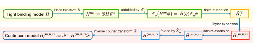
3. Derivation of continuum models from truncated reciprocal space models
In this section, we will propose an approximation scheme to obtain the higher order continuum models. As seen in Figure 3.1, we have obtained the truncated Hamiltonian by the Bloch transform, an unfolding procedure, and the reciprocal space truncation in Section 2. The next step is to perform the Taylor expansion at the Dirac points of the incommensurate Brillouin zone to obtain a polynomial approximation Hamiltonian . Subsequently, we will use a similar inverse process to derive the continuum model, including an infinite extension to define the Hamiltonian on , a folding process back to the momentum space, and the inverse Fourier transform to obtain the PDE form.
3.1. Taylor Expansion
We begin with a momenta polynomial approximation of (2.19). We note that the DoS (2.21) is an integral over the moiré Brillouin zone . We hence could only consider the behavior of the Hamiltonian in moiré reciprocal space. We rewrite (2.19) by the moiré reciprocal lattices and do the Taylor expansion around valley to obtain the polynomial approximation model.
Before expanding the Hamiltonian, we introduce the 2-dimensional multi-index notations for , and ,
Let and be the intralayer and interlayer expansion orders, respectively. For , we do the Taylor expansion for with respect to around ,
where we denote the -order Taylor polynomial approximation of by
For , , let
we do the Taylor expansion for with respect to around ,
where we denote the -order Taylor polynomial approximation of by
Hence, the polynomial approximation Hamiltonian is given by
| (3.24) |
where
and
We note that for and , we have . Since the Taylor expansion error scales as , the expansion accuracy will also be determined by the reciprocal space truncation. The following lemma gives the precise error analysis of the polynomial approximation.
Lemma 3.1.
Proof.
Proof is in Appendix A. ∎
3.2. Continuum Model
We now derive the continuum model from (3.24). It is not immediately obvious how to do this, as is defined on , while the continuum model is defined on . However, we find that the density of states of these models can be related as long as we focus on low energies, i.e., energies close to the monolayer Dirac energy. To make this precise, we have to extend the Hamiltonian to all of in such a way that it remains unchanged for small momenta (i.e., momenta close to the monolayer Dirac point), but becomes invertible for large momenta. We will then apply the inverse Fourier transform to obtain the continuum model.
Let , with smooth and 1 on , and compactly supported on with . We modify the expansion polynomials by
| (3.26) |
and denote the corresponding Hamiltonian parts by and . Then the infinite matrix is
The reason for modifying the expansion polynomials as in (3.26) is to ensure that is invertible for large , which will be important in the proofs below.
We notice that could be rewritten by the moiré reciprocal lattice, i.e., for ,
| (3.27) |
and for ,
| (3.28) |
where and for . We then define a map analogous to but sampled by moiré reciprocal lattices
and let
The following lemma gives the folding form of the approximation model.
Lemma 3.2.
We construct the operator decomposed sheet-wise as
| (3.29) |
to be the Hamiltonian such that for ,
The operator is composed of translation operators and multiplication operators given by
| (3.30) | |||
| (3.31) |
where for and .
Proof.
See Appendix B. ∎
Finally, let and . By the inverse Fourier transform, we obtain the continuum model for the valley
| (3.32) | ||||
We refer to this as the continuum model. We mention that the dependence is omitted in the continuum model Hamiltonian. This is because is mainly used to improve numerical efficiency, and is always chosen to ensure the momentum truncation converges. Therefore, does not fundamentally affect the accuracy of the continuum model.
In the following example, we can see that the BM model is a leading order continuum model. Therefore, we also refer to the continuum model as the BM model.
Example 3.1.
We consider the simplified TBG model in [22]. This simplified model has three nearest hoppings for the intralayer, and with a radial decay function for the interlayer such as (2.5). Specifically, the reciprocal space Hamiltonian for this model is
| (3.33) | ||||
We first derive the continuum model for the valley. We can easily obtain that
and
where . Here we use as the interlayer coupling since the three nearest hopping terms have equal strength. Then we have
where the matrices are
with , and the vectors are
The three vectors could also be explicitly given by
where is the distance between the Dirac points of the layers. We can see that for the valley has the same form as the BM model given in [6].
Observe that , we can immediately obtain the continuum model for the valley
where
3.3. Convergence of the Density of States
We finally discuss the convergence of the density of states of the continuum model. Similar with (2.21), that is approximated by
| (3.34) |
We can see that the error of comes from three parts: truncation error, polynomial approximation error, and smooth extension error. The first one has been given by Theorem 2.2, the second one can be estimated by Lemma 3.1, and the last one can be analyzed using the “ring decomposition technique” proposed by [16].
Theorem 3.1.
Assume Assumption 1 and assume TBG has hopping functions satisfying Assumption 2 and 3. Consider , , and . Let be the hopping truncation distance depending on . Let be the intralayer and interlayer expansion orders respectively. Then for , there are constants , , and corresponding to hopping truncation error, momenta truncation error, and Gaussian decay rates respectively, such that
| (3.35) | |||
where is a constant dependent of , and is a constant dependent of
| (3.36) |
Proof.
Proof is in Appendix C. ∎
We note that the constant for the polynomial approximation error scales as . Although we consider , since we only focus on a very small energy region around Dirac points, is still a small constant. We note as long as the hopping functions do not have asymptotic behavior with such as the inclusion of mechanical relaxation effects, which is the case for the simplified and wannier tight-binding models we consider, then [16].
4. Numerical Simulations
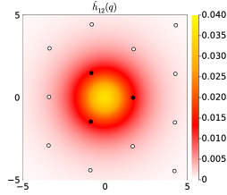
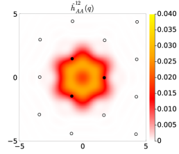
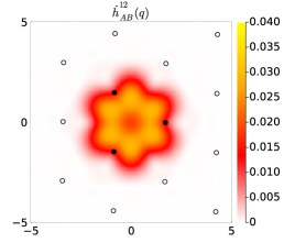
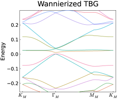
In this section, we shall give the high accuracy continuum models for the simplified TBG and the Wannierized TBG. We will demonstrate the conclusions by convergence results and band structures at the valley for the magic angle (). The results are similar for the valley. For the simplified TBG, we consider the model given by (3.33) and use the tight-binding parameters given in [6] and [22]. For the Wannierized TBG, we consider the monolayer tight-binding hopping parameters up to the fourth nearest neighbor, with values obtained from a previous first-principles study of graphene [12], and interlayer hopping coupling is also derived from the first-principles calculations [12]. As seen in Figure 4.2, the interlayer hopping couplings of these two TBG models have different decay and symmetry. Therefore, we can anticipate that their BM models will exhibit different accuracy on the band structure near the flat band, and their high-order corrections are also different.
In particular, we will use a more succinct method to truncate the reciprocal space for TBG. Let be the new momentum truncation parameter, then the basis set could be described by a fixed truncation radius
and the corresponding inclusion is . The reason for this is that the conical bands of graphene lead to a linear relationship between momentum cutoffs and energy range. We denote the high-symmetry lines of the moiré Brillouin zone at a single moiré valley by (, and define the relative error for momentum truncation along by
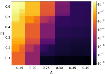
where and are the -th eigenvalues of and , respectively. In Figure 4.3, we show the relative error as a bi-variate function of and for the Wannierized TBG. We can observe that grows linearly with when converging, which validates the rational choice of . We also note that the error does not decrease continuously with , this is because the cardinality of increases piecewisely with .
In the following, all the simulations will use as the momentum truncation basis set. Since we are only concerned with the parameters selection for the continuum model, we will omit the subscript of momentum truncation (chosen to ensure the momentum truncation error converges) to simplify the notation.
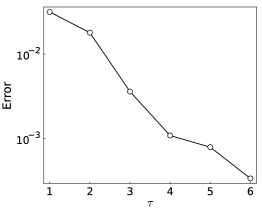
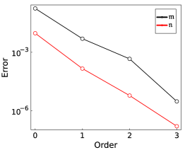
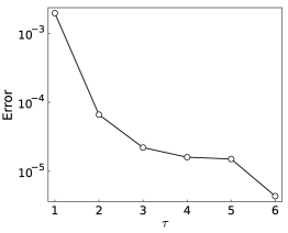
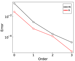
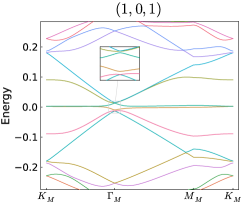
To select the “optimal” parameters for high accuracy models, we need to know the contribution of each parameter to convergence. Therefore, we first use the momentum space model as a reference and compare it with to evaluate the hopping truncation error. Next, we fix the hopping truncation parameter , and compare with () to evaluate the intralayer (interlayer) expansion error. Here, indicates that there is no polynomial approximation for the corresponding part. Figure 4.4 shows the relative errors for 6 electron eigenvalues closest to the Fermi energy along for three models. We observe that the errors decrease exponentially with , , , which is consistent with the convergence analysis. Although the model becomes more accurate with larger parameters, the model complexity is also higher. From the pictures, we can see that there are some “optimal” parameters to balance the trade-off. For example, we can take for the simplified TBG and for the Wannierized TBG, to achieve the desired accuracy without introducing too much complexity.
 |
 |
 |
 |
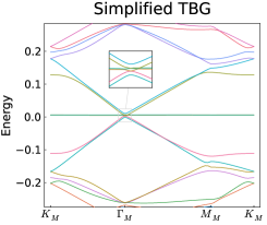
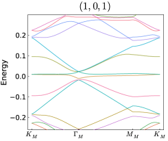
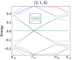
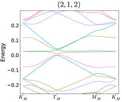
We further show the electronic band structures along for the momentum space model , the BM model , and the high accuracy model (with parameters chosen as above) respectively in Figure 4.5. For the simplified TBG, the momentum space model gives an extremely flat band very close to 0 energy. The BM model gives a slightly less flat band with a quite different band structure than the momentum space model. This indicates that the BM model of the simplified TBG can not accurately capture the characteristics at the magic angle. By increasing both the intralayer and interlayer expansion orders by one and the hopping truncation parameter by two, the band structure is almost identical to the exact result. Therefore, the parameter choices for the high accuracy continuum model are reasonable. For the Wannierized TBG, the band structure of the BM model is more identical to the exact result except for a slight shift towards 0. This explains why we can use smaller corrections to obtain the accurate mode for the Wannierized TBG compared to the simplified TBG.
 |
 |
 |
 |
 |
 |
Appendix A Proof of Lemma 3.1
Since the Taylor series of the hoppings are
and
By Assumption 2, 3 and the Cauchy–Schwarz inequality, we have
and
We can therefore obtain that the Taylor series converge absolutely for
Similarly, by the Taylor’s theorem, we have the following estimates for the remainders,
and
Let , for belonging to the above subset, we can obtain
where the constant is independent of .
Note that when and , we have . Then we view the matrix as blocks with respect to reciprocal lattices, we can have
Let be the sum of the absolute values of the non-diagonal entries in the -th row,
By the Gershgorin circle theorem , we can obtain
Appendix B Proof of Lemma 3.2
Appendix C Proof of Theorem 3.1
We denote the approximate DoS of by , and then divide the error into three parts:
Since the truncation part has been given by Theorem 2.2, we only need to quantify polynomial approximation error and extension error . For simplicity, we define the following notations to distinguish the intralayer part and interlayer par for a sheet-wise decomposed matrix ,
For the polynomial approximation error, we have
where and denote the -th eigenvalues of and respectively, and sorted in ascending order. Let be the dimensional subspace of . For any , , we have
where . Hence
By the min-max theorem, we obtain that for any ,
We hence have
In addition, we note that some error is also controlled by the Gaussian tail. Let be the -th eigenvalue of , we similarly have
where is definded in (2.15). Moreover, we separate the eigenvalues by energy windows. Consider an increasing collection of energy , satisfying . Then for , we have . Therefore, for such that , there is a constant such that
| (3.37) |
And by the conical structure of the monolayer band structure, we have
| (3.38) |
Then by (3.37) and (3.38), we obtain
We also note that
The analysis is similar for . Then by Lemma 3.1, we obtain
We now estimate . Since and have same hopping truncation and expansion orders, we could view and as fixed parameters. For simplicity of notations, we denote for matrices
so in particular,
Let be a contour around the spectrum such that . If the spectrum has gaps larger than , then would not be a simple curve in the complex plane but a union of one per ungapped interval of spectrum. We observe that
We use the ring decomposition technique from [16] to find the bound of . We define a new energy range
and a new enlarge strength
Consider an increasing collection of radii such that and . For , we write , and use (2.16), (2.18) to define the following decomposition:
We choose and such that if , then the decomposition gives a “nearest neighbor” decomposition. Since the sites are coupled in such a way that or , this can be easily achieved by choosing such that the index distance between the sites of two neighboring rings is proportional to
So we have the number of entries of each ring
| (3.39) |
We observe that the Hamiltonian is
We let be the matrix restricted to the rings through for , and be the corresponding inclusion. We also use the resolvent notations:
Then by (3.39),
| (3.40) | ||||
It suffices to show that for ,
| (3.41) |
| (3.42) |
In the following, we will omit the notation , and consider two cases for .
Case 1, : We divide into two regions,
| (3.43) |
where
We have
We observe that for , there is a such that
so the second term is bounded up by
| (3.44) |
Hence, it suffices to prove for arbitrary , there is a ,
| (3.45) |
Note that we can directly obtain (3.41) by taking for (C) and (3.45), and using . To obtain (3.45), we use the Schur complement for the ring decomposition
The last inequality is found by noting only couples ring on the left to ring on the right. We then rewrite using the top right entry in an iterative fashion as follows:
| (3.46) |
Recalling the definition of and ,
| (3.47) |
Then by (C) and (C), we obtain
for some .
Case 2, : We observe that
| (3.48) |
| (3.49) |
We first prove that the first term of (3.48) is bounded up by
Likewise, we divide into and as , but with
For the term, we have the same bound as for (C). Hence, it suffices to show that for ,
We observe
We next rewrite using the bottom left entry in an iterative fashion as follows:
By the same argument above
We next show that
We observe
Here the spectrum of can be approximated to increase linearly with . The reason for this is that for , the spectrum of is a conical structure, and only contains 1 order and negligible higher order modifications. We also have is bounded, since for large , is close to , and only contains 0 order and negligible higher order modifications. We then obtain
and
Using the same argument above, for , (3.49) is similarly bounded up by
References
- [1] Harry Bateman. Tables of integral transforms Volume 2. McGraw-Hill Book Company, 1954.
- [2] Simon Becker, Mark Embree, Jens Wittsten, and Maciej Zworski. Spectral characterization of magic angles in twisted bilayer graphene. Physical Review B, 103, 4 2021.
- [3] Simon Becker, Mark Embree, Jens Wittsten, and Maciej Zworski. Mathematics of magic angles in a model of twisted bilayer graphene. Probability and Mathematical Physics, 3:69–103, 2022.
- [4] Simon Becker, Tristan Humbert, and Maciej Zworski. Integrability in the chiral model of magic angles. arXiv:2208.01620, 2022.
- [5] B. Andrei Bernevig, Biao Lian, Aditya Cowsik, Fang Xie, Nicolas Regnault, and Zhi-Da Song. Twisted bilayer graphene. V. Exact analytic many-body excitations in Coulomb Hamiltonians: Charge gap, Goldstone modes, and absence of Cooper pairing. Phys. Rev. B, 103:205415, 2021.
- [6] Rafi Bistritzer and Allan H. MacDonald. Moiré bands in twisted double-layer graphene. Proceedings of the National Academy of Sciences of the United States of America, 108:12233–12237, 2011.
- [7] Éric Cancès, Louis Garrigue, and David Gontier. Simple derivation of moiré-scale continuous models for twisted bilayer graphene. Phys. Rev. B, 107:155403, 2023.
- [8] Éric Cancès and Long Meng. Semiclassical analysis of two-scale electronic Hamiltonians for twisted bilayer graphene. arXiv:2311.14011, 2023.
- [9] Yuan Cao, Valla Fatemi, Shiang Fang, Kenji Watanabe, Takashi Taniguchi, Efthimios Kaxiras, and Pablo Jarillo-Herrero. Unconventional superconductivity in magic-angle graphene superlattices. Nature, 556:43–50, 2018.
- [10] Trithep Devakul, Valentin Crépel, Yang Zhang, and Liang Fu. Magic in twisted transition metal dichalcogenide bilayers. Nature Communications, 12(1):6730, 2021.
- [11] Shiang Fang, Stephen Carr, Miguel A. Cazalilla, and Efthimios Kaxiras. Electronic structure theory of strained two-dimensional materials with hexagonal symmetry. Phys. Rev. B, 98:075106, 2018.
- [12] Shiang Fang and Efthimios Kaxiras. Electronic structure theory of weakly interacting bilayers. Phys. Rev. B, 93:235153, 2016.
- [13] Fabian M. Faulstich, Kevin D. Stubbs, Qinyi Zhu, Tomohiro Soejima, Rohit Dilip, Huanchen Zhai, Raehyun Kim, Michael P. Zaletel, Garnet Kin-Lic Chan, and Lin Lin. Interacting models for twisted bilayer graphene: A quantum chemistry approach. Phys. Rev. B, 107:235123, Jun 2023.
- [14] Zeyu Hao, A. M. Zimmerman, Patrick Ledwith, Eslam Khalaf, Danial Haie Najafabadi, Kenji Watanabe, Takashi Taniguchi, Ashvin Vishwanath, and Philip Kim. Electric field–tunable superconductivity in alternating-twist magic-angle trilayer graphene. Science, 371(6534):1133–1138, 2021.
- [15] Mikito Koshino and Nguyen N.T. Nam. Effective continuum model for relaxed twisted bilayer graphene and moiré electron-phonon interaction. Phys. Rev. B, 101, 5 2020.
- [16] Daniel Massatt, Stephen Carr, and Mitchell Luskin. Electronic observables for relaxed bilayer two-dimensional heterostructures in momentum space. Multiscale Modeling & Simulation, 21(4):1344–1378, 2023.
- [17] Daniel Massatt, Stephen Carr, Mitchell Luskin, and Christoph Ortner. Incommensurate heterostructures in momentum space. Multiscale Modeling & Simulation, 16:429–451, 2018.
- [18] Naoto Nakatsuji, Takuto Kawakami, and Mikito Koshino. Multiscale lattice relaxation in general twisted trilayer graphenes. Phys. Rev. X, 13:041007, 2023.
- [19] Mariya Romanova and Vojtěch Vlček. Stochastic many-body calculations of moiré states in twisted bilayer graphene at high pressures. npj Computational Materials, 8(1):11, 2022.
- [20] Grigory Tarnopolsky, Alex Jura Kruchkov, and Ashvin Vishwanath. Origin of magic angles in twisted bilayer graphene. Physical Review Letters, 122, 2019.
- [21] Ting Wang, Huajie Chen, Aihui Zhou, Yuzhi Zhou, and Daniel Massatt. Convergence of the planewave approximations for quantum incommensurate systems. arXiv:2204.00994, 2024.
- [22] Alexander B. Watson, Tianyu Kong, Allan H. MacDonald, and Mitchell Luskin. Bistritzer–MacDonald dynamics in twisted bilayer graphene. Journal of Mathematical Physics, 64(3):031502, 03 2023.
- [23] Alexander B. Watson and Mitchell Luskin. Existence of the first magic angle for the chiral model of bilayer graphene. Journal of Mathematical Physics, 091502, 2021.
- [24] Xi Zhang, Kan-Ting Tsai, Ziyan Zhu, Wei Ren, Yujie Luo, Stephen Carr, Mitchell Luskin, Efthimios Kaxiras, and Ke Wang. Correlated insulating states and transport signature of superconductivity in twisted trilayer graphene superlattices. Phys. Rev. Lett., 127:166802, 2021.