Generalized Type II Fusion of Cluster States

Noam Rimock, Khen Cohen and Yaron Oz School of Physics and Astronomy, Tel Aviv University, Ramat Aviv 69978, Israel
Abstract

Measurement based quantum computation is a quantum computing paradigm, that employs single-qubit measurements performed on an entangled resource state in the form of a cluster state. A basic ingredient in the construction of the resource state is the type II fusion procedure, which connects two cluster states. We generalize the type II fusion procedure by generalizing the fusion matrix, and classify the resulting final states, which also include cluster states up to single-qubit rotations. We prove that the probability for the success of the generalized type II fusion is bounded by fifty percent, and classify all the possibilities to saturate the bound. We analyze the enhancement of the fusion success probability above the fifty percent bound, by the reduction of the entanglement entropy of the fusion link. We prove that the only states, that can be obtained with hundred percent probability of succces, are product states.

I Introduction

Refer to caption
Figure 1: Generalized type II Fusion of cluster states: The higher the probability for the success of the fusion process, the lower the entanglement entropy of the two qubits connecting the clusters.

Measurement based quantum computation (MBQC) is a quantum computing paradigm harnessing entanglement and single-qubit measurements to perform general quantum computational tasks MBQCfirstArticle ; MBQC2009 . MBQC is an alternative framework to the quantum circuit computation model, which is realized naturally in photonic platforms. At its core, MBQC employs single-qubit measurements performed on an entangled resource state MBQConClusterStatesFirstArticle ; MBQC2021 , often a cluster state ClusterStatesNielsen ; ClusterStatesOriginalPaper where neighboring qubits, each in a superposition state, are entangled by a CZ gate (for an experimental realization see e.g. RealizatonOfMBQC0 ; RealizatonOfMBQC1 ; RealizatonOfMBQC2 ; RealizatonOfMBQC3 ). MBQC on cluster states is a universal quantum computation model that is isomorphic to the quantum circuit computation one.

The construction of cluster states is the first step for applying MBQC, and a fundamental ingredient for this task is the fusion gate, which is used to connect resource states. Fusion gates were introduced in KLMprotocolNature ; UsingAncillae0 and in NielsenProtocolFirstArticle ; YoranReznikProtocalFirstArticle . Two types of fusion protocols, I and II, were proposed in BrowneRudolph . Type II fusion is based on qubit measurements, hence it is a probablistic procedure. Given two cluster states that one wishes to fuse, the type II fusion is basically a measurement of two qubits, one from each cluster. There are two outcomes depending on the measurement result: (i) the size of the resulting cluster state is the sum of the sizes of the two cluster states minus the two measured qubit, (ii) the two cluster states remain separated, each losing one qubit. The probability for the success of type II fusion, i.e. result (i), is bounded by fifty percent.

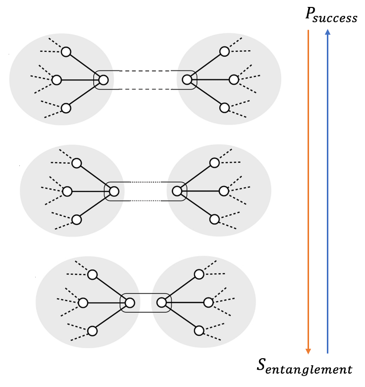
Type II fusion is fundamental for the construction of a two-dimensional cluster state denoted by $L$-shape BrowneRudolph , from one-dimensional ones. This is necessary in order to have a quantum advantage, since MBQC performed on one-dimensional clusters is as effective as a classical probablistic computational model. The construction of an $L$-shape cluster state costs on average no more than $52$ bell pairs BrowneRudolph . This number can be reduced if one increases the probability of fusion success, which is feasible if we reduce the entanglement entropy of the fusion link, see Fig. 1. Type II fusion based on Bell state measurement (BSM) FusionBasedQC ; ThreePhoton has been proven to have a maximal value of fifty percent probability of success, when using only linear elements. i.e. that can be realized via linear optics elements MaxEfficiency ; BellMeasurements . This success probability can be improved by adding ancilla resources UsingAncillae0 ; UsingAncillae1 ; UsingAncillae2 ; UsingAncillae3 ; UsingAncillae4 . The proof of MaxEfficiency required one of the four standard Bell states to be the final state of the fusion, which in particular means having a fusion link with a maximal value of entanglement entropy.

In this work we generalize the standard type II fusion procedure, by generalizing the fusion matrix, and classify the resulting final states as cluster states, stabilizer states, cluster states up to one-qubit rotations and Weighted graph states. In particular, we generalize the proof of MaxEfficiency , by relaxing the final state condition, and allow having a general maximally entangled final state. We prove that the success probability of the generalized type II fusion is bounded by fifty percent, and provide a precise mathematical description of all the ways to saturate the bound. We analyze the cases of non maximally entangled fusion links, and perform a numerical optimization analysis of fusion gates, allowing lower entanglement entropy and obtaining higher probability of fusion success.

The paper is organized as follows: In section II we briefly review cluster states and type II fusion. In Section III we generalize type II fusion, and classify the final states that arise from this fusion. In section IV we consider the possibility of reducing the entanglement entropy of the fusion link. We define the fusion problem as a mathematical optimization problem, and correlate the fusion success probabilities and the values of the entanglement entropies. We show that allowing a reduction in the entanglement entropy of the fusion link, allows for an increase in the fusion success probability. In Section V we conduct an analytical analysis and prove the fifty percent probability success bound for a maximal entanglement entropy as well deriving several other results. In Section VI we outline our numerical optimization method, followed by a demonstration of the fusion probability success versus the link entanglement entropy. Section VII is devoted to a discussion and an outlook. Detailed proofs of the theorems are given in the various appendices.

II Cluster States and Type II Fusion

In this section we will briefly review the definitions of stabilizer states, graph states and cluster states and the process of type II fusion. Detailed reviews of optical quantum computing can be found in ReviewOfOpticalQuantumComputing0 ; ReviewOfOpticalQuantumComputing1 ; 5lectures .

II.1 Stabilizer States

A state $\ket{\phi}$ of $n$ qubits is called a stabilizer state, if there exists a subgroup $S$ of the Pauli group with $n$ generators ($|S|=2^{n}$) such that for any operator $A\in S$, $A\ket{\phi}=\ket{\phi}$. If $g_{1},g_{2},...g_{n}$ are the generators of $S$ then an equivalent requirement is $g_{i}\ket{\phi}=\ket{\phi}$ for every $1\leq i\leq n$, and $g_{i}$ are called stabilizers. The set of stabilizer states is the set of all the states that can be obtained by acting on $\ket{0}^{\otimes n}$ with elements of the Clifford algebra GeneralizedGraphStatesAndStabilizerStates .

For instance, the two-qubit state ($a$ and $b$ denote the qubits):

$$\displaystyle\frac{1}{\sqrt{2}}(\ket{0}_{a}\ket{+}_{b}+\ket{1}_{a}\ket{-}_{b})\ ,$$ (1)

is a stabilizer state, with the generators:

$$\displaystyle g_{1}=X_{a}Z_{b},\leavevmode\nobreak\ \leavevmode\nobreak\ g_{2}=X_{b}Z_{a}\ ,$$ (2)

where $X,Z$ are the Pauli matrices.

II.2 Weighted Graph States

Refer to caption
Figure 2: Graph states: (a) A graph state is generated by assigning to each node a single qubit in the state $\ket{+}$, and applying a $CZ$ gate to two neighboring (connected by an edge) vertices $i,j$. This construction can be described recursively as follows. Choose a vertex $a$ in the graph, set the qubits without $a$ and its edges in the graph state $\ket{\phi}_{V\setminus\{a\}}$, and apply $CZ$ gates to $a$ and its neighbors. The resulting graph state is as in Eq. (6). We denote by $K_{a}$ the stabilizer of qubit $a$, and the graph wave function is an eigenstate of this stabilizer with eigenvalue $1$. (b) Examples of one-dimensional graph states of $n=2,3,4$ qubits. The corresponding wave functions are evaluated recursively using Eq. (6).

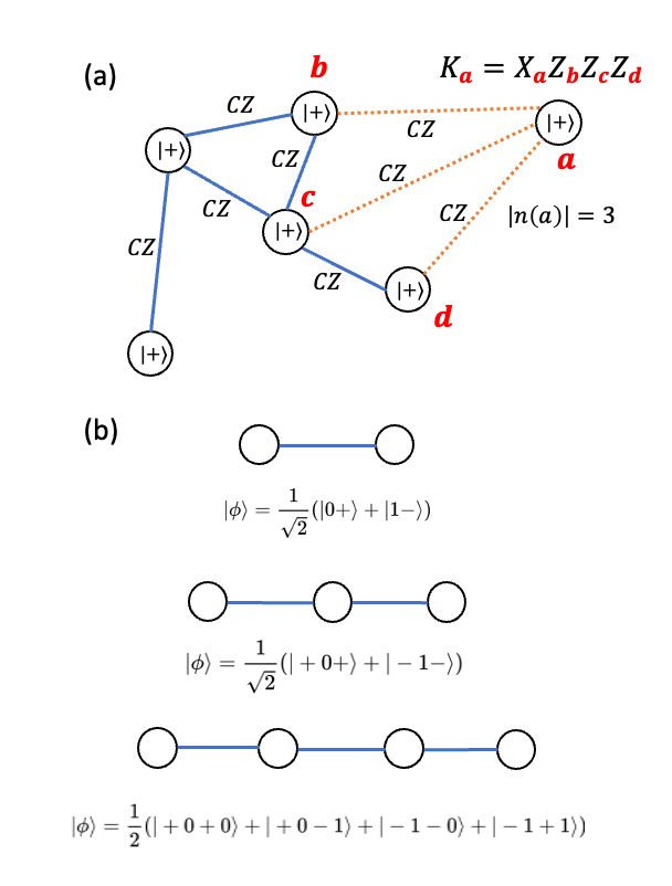
Given a graph GraphTheoryBook with a set of vertices $V$ and a set of edges $E$, one associates to it a graph state as follows. We assign to each vertex a qubit in the superposition state $\ket{+}=\frac{1}{\sqrt{2}}(\ket{0}+\ket{1})$, and apply a $CZ$ gate to every two qubits $i,j$ that are connected by an edge:

$$\displaystyle\ket{\phi}=\prod_{(i,j)\in E}CZ^{i,j}\prod_{k}\ket{+}_{k}\ .$$ (3)

Since the $CZ$ gates commute with each other, the order of the application them is irrelevant. The resulting state is called a graph state. For instance, the graph state of two qubits connected by an edge reads:

$$\displaystyle CZ\ket{+}\ket{+}=\frac{1}{\sqrt{2}}(\ket{0}\ket{+}+\ket{1}\ket{-})\ ,$$ (4)

and is the stabilizer state (1).

Graph states have an equivalent definition as a stabilizer states of the subgroup $S$ of the Pauli group generated by $K_{a}$:

$\displaystyle K_{a}\ket{\phi}$ $\displaystyle=$ $\displaystyle\ket{\phi},$
$\displaystyle K_{a}$ $\displaystyle=$ $\displaystyle X_{a}\otimes\prod_{b\in n(a)}Z_{b}\ ,$ (5)

where $X_{a}$ and $Z_{b}$ are Pauli operators acting on the qubits labelled by $a$ and $b$, respectively, and $n(a)$ denotes the vertices connected to $a$. The mutually commuting generators $K_{a}(K_{a}^{2}=I_{d}$) are the stabilizers of the state $\ket{\phi}$.

The construction of graph states can be defined recursively as follows. Choose a vertex $a$ in the graph, denote the graph state wave function without this vertex and without the edges that are connected to it as $\ket{\phi}_{V\setminus\{a\}}$. Then, add the vertex $a$ to the graph and apply $CZ$ gates to $a$ and its neighbors $n(a)$. The resulting graph state wave function reads:

$$\displaystyle\ket{\phi}=\frac{1}{\sqrt{2}}(\ket{0}_{a}\ket{\phi}_{V\setminus\{a\}}+\ket{1}_{a}\prod_{b\in n(a)}Z_{b}\ket{\phi}_{V\setminus\{a\}})\ .$$ (6)

In order to complete the recursive construction, we take in the first step the single-qubit the wave function to be $\ket{+}$. For simplicity, in the following we will omit the $\frac{1}{\sqrt{2}}$ factor and absorb it in $\ket{\phi}_{V\setminus\{a\}}$. For completeness, we include the proof of the equivalence of (5) and (6) in appendix B.

One can generalize the definition of the graph states as follows. Consider a graph with $V$ vertices and $E$ edges. Assign a qubit in the state $\ket{+}$ to each vertex and apply to each pair of qubits connected by an edge a two-qubit gate, which is not the global phase gate and not necessarily $CZ$. The set of two-qubits gates must be commuting so that the order of their application becomes irrelevant. Also, all the gates must differ from the global phase gate, otherwise they will trivially commute with all the other gates and generate a product state of two subgraphs. The resulting state is called a weighted graph state hein2004multiparty ; dur2005entanglement .

By applying Pauli $Z$ rotations on the qubits, one can recast the two-qubit gates acting on qubits $a$ and $b$ in the form GeneralizedGraphStatesAndStabilizerStates :

$$\displaystyle U_{ab}=e^{i\chi_{ab}\ket{1_{a},1_{b}}\bra{1_{a},1_{b}}}=\ket{0_{a},0_{b}}\bra{0_{a},0_{b}}+\ket{0_{a},1_{b}}\bra{0_{a},1_{b}}$$
$$\displaystyle+\ket{1_{a},0_{b}}\bra{1_{a},0_{b}}+e^{i\chi_{ab}}\ket{1_{a},1_{b}}\bra{1_{a},1_{b}}\ .$$ (7)

As will be shown later, the requirement for maximal entanglement between two connected qubits implies that $\chi_{ab}=\pi$ GeneralizedGraphStatesAndStabilizerStates .

II.3 Cluster States

A cluster state of size $N$ is an entangled state of $N$ qubits that can be represented as a graph with $N$ vertices, where each vertex denotes a qubit, and an edge connecting two vertices corresponds to an entangling $CZ$ gate that acts on the corresponding qubits. A cluster state can be specified by the stablizers:

$\displaystyle K_{a}\ket{\phi}$ $\displaystyle=$ $\displaystyle(-1)^{k_{a}}\ket{\phi},\leavevmode\nobreak\ \leavevmode\nobreak\ \leavevmode\nobreak\ k_{a}\in\{0,1\},$
$\displaystyle K_{a}$ $\displaystyle=$ $\displaystyle X_{a}\otimes\prod_{b\in n(a)}Z_{b}\ .$ (8)

Graph states are particular examples of cluster states, where difference between (8) and (5) are $\{k_{a}\}$, which are zero for a graph state. $Z_{a}$ commutes $K_{b}$ when aβ‰ bπ‘Žπ‘a\neq b and anticommutes with $K_{a}$. Thus, one can construct any cluster state from a corresponding graph state by acting with $Z_{a}$ on each vertex $a$ where $k_{a}=1$. As with graph states, the cluster state wave function can be constructed recursively. Choose a vertex $a$ in the graph, and denote the wave function without this vertex and without the edges that are connected to it as $\ket{\phi}_{V\setminus\{a\}}$. Next, we add the vertex $a$ to the graph and if $k_{a}=0$ we act with $CZ$ gates on the qubit $a$ and its neighbors $n(a)$, which results in the recursive relation (6). If $k_{a}=1$ we act on $a$ with the $Z_{a}$ gate.

II.4 Type II Fusion

We will work within the linear optics framework, where a qubit is realized by a photon with a fixed frequency, and the quantum state is encoded in the photon’s polarization, where $|0\rangle$ and $|1\rangle$ correspond to horizontal and vertical polarizations, respectively PhotonicQubits . The photon creation operators a†=(aH†,aV†)superscriptπ‘Žβ€ subscriptsuperscriptπ‘Žβ€ π»subscriptsuperscriptπ‘Žβ€ π‘‰a^{\dagger}=(a^{\dagger}_{H},a^{\dagger}_{V}) are defined, such that aH†subscriptsuperscriptπ‘Žβ€ π»a^{\dagger}_{H} or aV†subscriptsuperscriptπ‘Žβ€ π‘‰a^{\dagger}_{V} acting on the vacuum state $|0\rangle$, create a photon with a horizontal or vertical polarization, respectively. A wave function $|\Psi\rangle={\cal O}|0\rangle$ will be denoted by the operator ${\cal O}$ made of the photon creation operators. For instance, a two-qubit Bell state reads in this notation:

|B​e​l​l⟩:12​(aH†​bH†+aV†​bV†).:ket𝐡𝑒𝑙𝑙12subscriptsuperscriptπ‘Žβ€ π»subscriptsuperscript𝑏†𝐻subscriptsuperscriptπ‘Žβ€ π‘‰subscriptsuperscript𝑏†𝑉|Bell\rangle:\frac{1}{\sqrt{2}}\left(a^{{\dagger}}_{H}b^{{\dagger}}_{H}+a^{{\dagger}}_{V}b^{{\dagger}}_{V}\right)\ . (9)

The entangling gates are realized by linear optics elements and measurements, and are therefor probabilistic. One constructs a larger cluster state from smaller ones, by employing probabilistic fusion gates. In the following, we will focus on type II fusion gates.

Refer to caption
Figure 3: Type II fusion optical setup, where $a$ and $b$ are the incoming photon modes that pass a diagonal polarization beam splitter and exit as $c$ and $d$ modes which are measured by the detectors $D_{2}$ and $D_{1}$.

Consider two cluster states, whose wave functions are denoted by the operators $\hat{C_{1}}$ and $\hat{C_{2}}$, and we mark one photon in each one of them, $a$ and $b$ respectively:

C1^=12​(f1​aH†+f2​aV†),C2^=12​(f3​bH†+f4​bV†).formulae-sequence^subscript𝐢112subscript𝑓1subscriptsuperscriptπ‘Žβ€ π»subscript𝑓2subscriptsuperscriptπ‘Žβ€ π‘‰^subscript𝐢212subscript𝑓3subscriptsuperscript𝑏†𝐻subscript𝑓4subscriptsuperscript𝑏†𝑉\displaystyle\hat{C_{1}}=\frac{1}{\sqrt{2}}(f_{1}a^{\dagger}_{H}+f_{2}a^{\dagger}_{V}),\hskip 14.22636pt\hat{C_{2}}=\frac{1}{\sqrt{2}}(f_{3}b^{\dagger}_{H}+f_{4}b^{\dagger}_{V})\ . (10)

a†superscriptπ‘Žβ€ a^{\dagger} and $b^{\dagger}$ are the creation operators of the marked photons and $f_{i},i=1,2,3,4$ denote the other parts of the two cluster states. The product state of these two cluster states reads:

C1^​C2^=12​(f1​aH†+f2​aV†)​(f3​bH†+f4​bV†)^subscript𝐢1^subscript𝐢212subscript𝑓1subscriptsuperscriptπ‘Žβ€ π»subscript𝑓2subscriptsuperscriptπ‘Žβ€ π‘‰subscript𝑓3subscriptsuperscript𝑏†𝐻subscript𝑓4subscriptsuperscript𝑏†𝑉\displaystyle\hat{C_{1}}\hat{C_{2}}=\frac{1}{2}\left(f_{1}a^{\dagger}_{H}+f_{2}a^{\dagger}_{V}\right)\left(f_{3}b^{\dagger}_{H}+f_{4}b^{\dagger}_{V}\right)
=12​(f1​f3​aH†​bH†+f2​f3​aV†​bH†+f1​f4​aH†​bV†+f2​f4​aV†​bV†).absent12subscript𝑓1subscript𝑓3subscriptsuperscriptπ‘Žβ€ π»subscriptsuperscript𝑏†𝐻subscript𝑓2subscript𝑓3subscriptsuperscriptπ‘Žβ€ π‘‰subscriptsuperscript𝑏†𝐻subscript𝑓1subscript𝑓4subscriptsuperscriptπ‘Žβ€ π»subscriptsuperscript𝑏†𝑉subscript𝑓2subscript𝑓4subscriptsuperscriptπ‘Žβ€ π‘‰subscriptsuperscript𝑏†𝑉\displaystyle=\frac{1}{2}(f_{1}f_{3}a^{\dagger}_{H}b^{\dagger}_{H}+f_{2}f_{3}a^{\dagger}_{V}b^{\dagger}_{H}+f_{1}f_{4}a^{\dagger}_{H}b^{\dagger}_{V}+f_{2}f_{4}a^{\dagger}_{V}b^{\dagger}_{V})\ . (11)

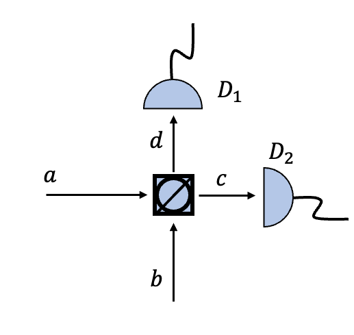
In the optical Type II fusion setup we pass two photons through a diagonal polarization beam splitter (PBS2), as in Figure 3, and the output modes read:

$\displaystyle c_{H}$ $\displaystyle=$ $\displaystyle\frac{1}{2}(a_{H}+a_{V}+b_{H}-b_{V}),$
$\displaystyle c_{V}$ $\displaystyle=$ $\displaystyle\frac{1}{2}(a_{H}+a_{V}-b_{H}+b_{V}),$
$\displaystyle d_{H}$ $\displaystyle=$ $\displaystyle\frac{1}{2}(a_{H}-a_{V}+b_{H}+b_{V}),$
$\displaystyle d_{V}$ $\displaystyle=$ $\displaystyle\frac{1}{2}(-a_{H}+a_{V}+b_{H}+b_{V})\ .$ (12)

Substituting (12) in (11) gives the state of the two clusters in terms of $c,d$ (up to normalization):

$$\displaystyle(f_{1}+f_{2})(f_{3}-f_{4})({c_{H}^{{\dagger}}}^{2}-{c_{V}^{{\dagger}}}^{2})$$
$$\displaystyle+(f_{1}-f_{2})(f_{3}+f_{4})({d_{H}^{{\dagger}}}^{2}-{d_{V}^{{\dagger}}}^{2})$$
$$\displaystyle+2(f_{1}f_{3}+f_{2}f_{4})c_{H}^{{\dagger}}d_{H}^{{\dagger}}+2(f_{1}f_{4}+f_{2}f_{3})c_{H}^{{\dagger}}d_{V}^{{\dagger}}$$
$$\displaystyle+2(f_{1}f_{4}+f_{2}f_{3})c_{V}^{{\dagger}}d_{H}^{{\dagger}}+2(f_{1}f_{3}+f_{2}f_{4})c_{V}^{{\dagger}}d_{V}^{{\dagger}}\ .$$ (13)

Measuring the output photons, there is a probability $\frac{1}{2}$ to measure two photons at the same output port, $c$ or $d$, and having the same polarization $H$ or $V$. In such a case, the resulting wave functions are:

$\displaystyle\frac{1}{2}(f_{1}+f_{2})(f_{3}-f_{4})\leavevmode\nobreak\ or\leavevmode\nobreak\ \frac{1}{2}(f_{1}-f_{2})(f_{3}+f_{4})\ ,$ (14)

which are separable states. There is also a $\frac{1}{2}$ probability to measure one output photon in each port, one in $c$ and one in $d$, where they can be in an H or V state. The resulting wave functions read:

$\displaystyle\frac{1}{\sqrt{2}}(f_{1}f_{3}+f_{2}f_{4})\leavevmode\nobreak\ or\leavevmode\nobreak\ \frac{1}{\sqrt{2}}(f_{1}f_{4}+f_{2}f_{3})\ ,$ (15)

which are the required Bell type entanglement between the two clusters. Thus, this procedure yields a maximal entanglement with a $\frac{1}{2}$ probability of success 111For further reading see 5lectures ; BrowneRudolph ; stanisic2015universal . We use the same notations as in 5lectures ..

Refer to caption
Figure 4: Type II Fusion: (a) Two one-dimensional clusters. An $X$ measurement is performed on a qubit that belongs to one of the clusters, erases it and connects its two neighbors $a$ and $e$ to one logical qubit $L$. (b) Type II fusion is performed on qubit $a$ in $L$ and qubit $b$ from the second cluster. (c) The result of the fusion: qubits $a,b$ are deleted, and qubit $e$ is connected to the previous neighbors $n(L)$ of the logical qubit $L$, and to the previous neighbors $n(b)$ of the qubit $b$.

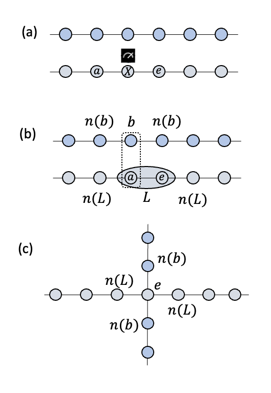
The Type II fusion plotted in Figure 4 is used for the construction of an $L$-shape cluster state in order to build a two-dimensional cluster from one-dimensional ones. Step (a): one begins with two one-dimensional clusters, and performs an $X$ measurement on one of the qubits of one of the two clusters. This erases the qubit from the cluster, and combines its two neighbors $a$ and $e$. Step (b): one combines $a,e$ qubits to one logical qubit $L$:

$$\displaystyle\ket{0}_{L}=\ket{0}_{a}\ket{0}_{e}\hskip 14.22636pt\ket{1}_{L}=\ket{1}_{a}\ket{1}_{e}\ ,$$ (16)

and denotes by $b$ a qubit from the second cluster. Using the recursive relation in (6), the total wave function takes the form:

$\displaystyle\ket{\phi}=\left(\ket{0}_{L}\ket{\phi_{L}}_{V\setminus\{L\}}+\ket{1}_{L}\prod_{c\in n(L)}Z_{c}\ket{\phi_{L}}_{V\setminus\{L\}}\right)$
$\displaystyle\left(\ket{0}_{b}\ket{\phi_{b}}_{V\setminus\{b\}}+\ket{1}_{b}\prod_{d\in n(b)}Z_{d}\ket{\phi_{b}}_{V\setminus\{b\}}\right)\ ,$ (17)

where $n(L),n(b)$ denote the neighbors of quits $L$ and $b$, and we use for simplicity of notation the same $V$ to denote the set of all the qubits in the clusters corresponding to $L$ and $b$. Note, that we assumed that $k_{a}=k_{b}=0$, but this can be modified by acting with $Z_{a}$ and $Z_{b}$.

A successful type II fusion on the qubits $a$ and $b$ is defined as: operating with:

$${\rm Type}\leavevmode\nobreak\ {\rm II}:\leavevmode\nobreak\ \bra{0}_{a}\bra{0}_{b}+\bra{1}_{a}\bra{1}_{b}\leavevmode\nobreak\ or\leavevmode\nobreak\ \bra{0}_{a}\bra{1}_{b}+\bra{1}_{a}\bra{0}_{b}\ .$$ (18)

Operating with $\bra{0}_{a}\bra{0}_{b}+\bra{1}_{a}\bra{1}_{b}$ yields the state:

$$\displaystyle\ket{0}_{e}\ket{\phi_{L}}_{V\setminus\{L\}}\ket{\phi_{b}}_{V\setminus\{b\}}+$$
$$\displaystyle+\ket{1}_{e}\prod_{c\in n(L)}Z_{c}\ket{\phi_{L}}_{V\setminus\{L\}}\prod_{d\in n(b)}Z_{d}\ket{\phi_{b}}_{V\setminus\{b\}}\ ,$$ (19)

which is the cluster state (c), as in the recursive definition (6). In the new cluster, $e$ is connected both to the previous neighbouring qubits of the logical qubit $L$, as well as to the neighbouring qubits of $b$, and have $k_{e}=0$ while it remains unchanged for all the other qubits.

Operating with $\bra{0}_{a}\bra{1}_{b}+\bra{1}_{a}\bra{0}_{b}$ yields the state:

$$\displaystyle\ket{0}_{e}\ket{\phi}_{V\setminus\{L\}}\prod_{d\in n(b)}Z_{d}\ket{\phi}_{V\setminus\{b\}}+$$
$$\displaystyle+\ket{1}_{e}\prod_{c\in n(L)}Z_{c}\ket{\phi}_{V\setminus\{L\}}\ket{\phi}_{V\setminus\{b\}}\ ,$$ (20)

which is a cluster state, having the same structure as in Figure 4 (c), but with different eigenvalues of the stabilizers in (8) compared to (19): for all the qubits $d\in n(b)$, $(-1)^{k_{d}}$ change their sign, because this state is obtained from (19) by operating with $Z_{d}$ on all $d\in n(b)$. Thus, if one connects two graph states and aims at a resulting graph state, an action with $Z_{d}$ on all $d\in n(b)$:

$$\ket{\phi^{\prime}}_{V\setminus\{b\}}=\prod_{d\in n(b)}Z_{d}\ket{\phi}_{V\setminus\{b\}}\ ,$$ (21)

is needed. Substituting this in (20) using $Z^{2}=I$ gives a state of the form of (19).

III Generalized Type II Fusion and the Final States

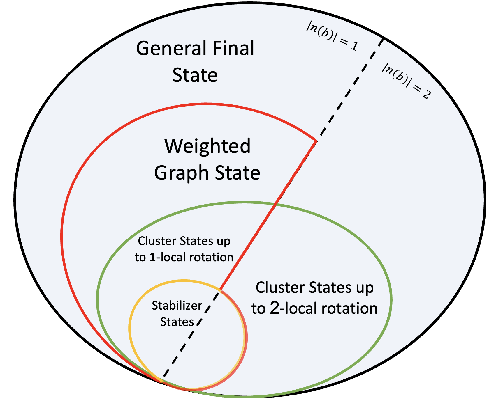
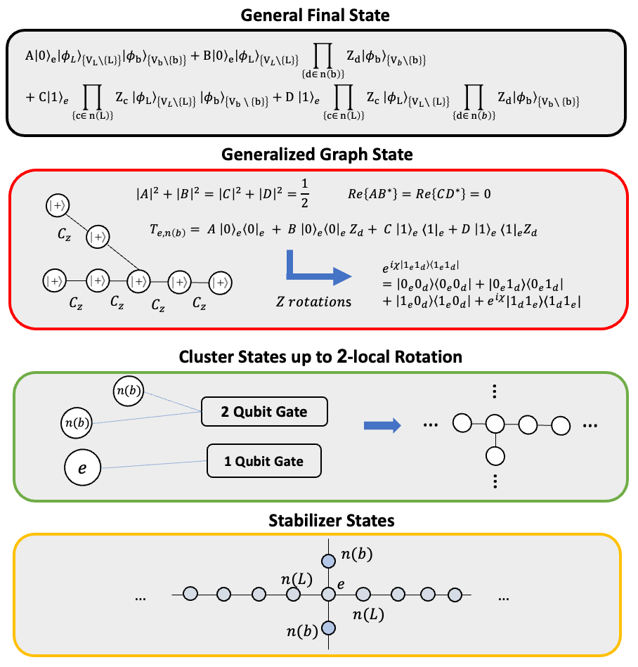
In the following we introduce a generalization of type II fusion, and prove three theorems on the conditions needed to obtain a stabilizer state, a Weighted graph state or a cluster state up to two-qubit rotations. The results of the theorems are summarized in Figure 5, and by the explicit formulas in Figure 13 in section D in the appendix.

Consider Figure 5. There is the set of all the possible final states of the two fused clusters, which are not necessarily cluster states. Within this general set we define three classes of final states. The first class consists of stabilizer states, which we consider in theorem 1, where we can operate with a phase shift gate on qubit $e$ to generate a cluster state. The set of stabilizer states is marked by yellow in Figure 5.

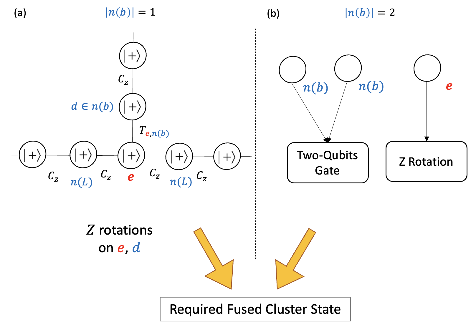
The second class consists of Weighted graph states having the same structure as the required fused cluster states. There are two cases, which we consider in theorem 2: (i) $|n(b)|=2$, which means that the qubit $b$ that we fuse is from the middle of its cluster. Then, every Weighted graph state with the same structure is also a stabilizer state. (ii) $|n(b)|=1$, which means that the qubit $b$ that we fuse is from the edge of its cluster. Then, the final states are also cluster states up to two-qubit rotations. Note, however, that such a cluster state can be generated also by applying one $CZ$ gate. The set of Weighted graph states is marked by red in Figure 5.

The third class consists of cluster states up to two-qubit rotations, when $|n(b)|=2$, and one-qubit rotations, when $|n(b)|=1$. This is a set of states that can take the form of the cluster state by operating with two-qubits gates on $n(b)$ and a single qubit gate on $e$ in the case $|n(b)|=2$, and single qubit gates on $n(b)$ and a single qubit gate on $e$ when $|n(b)|=1$. The case $|n(b)|=1$ is very useful. The case $|n(b)|=2$ is less useful, as it requires the application of a 2-qubit gate, which however is still less than the three $CZ$ gates, that need to be applied in order to construct the required fused cluster state from the original one-dimensional clusters without fusion. In theorem 3 we identify these states and prove that if $|n(b)|=1$, then they are Weighted graph states. In theorem 4 we prove that when $|n(b)|=1$, it includes all the Weighted graph states with maximal entanglement entropy. This set of states that are cluster states up to two-qubit rotations or one-qubit rotations is marked by green in Figure 5.

Figure 5 shows the hierarchy of the sets of final states after fusion. The outer set is divided by a line to two subsets for the cases $|n(b)|=1$ and $|n(b)|=2$, corresponding to the cases where the qubit $b$ is or is not at the end of its one-dimensional cluster before the fusion, respectively. When $|n(b)|=1$, the yellow set of stabilizer states is a subset of the green set, that includes cluster states up to one-qubit rotations, which is a subset of the red set of Weighted graph states. When $|n(b)|=2$, the yellow set of stabilizers states is identified with the red set of Weighted graph states, and is as subset of the green set of cluster states up to a two-qubit rotation.

III.1 Generalized Type II Fusion

Refer to caption
Figure 5: All the possible final states after performing a generalized type II fusion. The black outer set is the set of all the final states. The yellow set is the set of all the final states that are stabilizer states. The red set is the set of all the final states that are Weighted graph states. The green set is the set of all the final states that are cluster states up to two-qubit rotations when $|n(b)|=2$, and one-qubit rotations when $|n(b)|=1$.

Consider two incoming photons and linear optics devices. The transformation of the creation operators is unitary $U$ CreatingU0 ; CreatingU1 ; CreatingU2 :

[aH†aV†bH†bV†]=[U11U12U13U14U21U22U23U24U31U32U33U34U41U42U43U44]​[cH†cV†dH†dV†].matrixsubscriptsuperscriptπ‘Žβ€ π»subscriptsuperscriptπ‘Žβ€ π‘‰subscriptsuperscript𝑏†𝐻subscriptsuperscript𝑏†𝑉matrixsubscriptπ‘ˆ11subscriptπ‘ˆ12subscriptπ‘ˆ13subscriptπ‘ˆ14subscriptπ‘ˆ21subscriptπ‘ˆ22subscriptπ‘ˆ23subscriptπ‘ˆ24subscriptπ‘ˆ31subscriptπ‘ˆ32subscriptπ‘ˆ33subscriptπ‘ˆ34subscriptπ‘ˆ41subscriptπ‘ˆ42subscriptπ‘ˆ43subscriptπ‘ˆ44matrixsubscriptsuperscript𝑐†𝐻subscriptsuperscript𝑐†𝑉subscriptsuperscript𝑑†𝐻subscriptsuperscript𝑑†𝑉\begin{bmatrix}a^{\dagger}_{H}\\ a^{\dagger}_{V}\\ b^{\dagger}_{H}\\ b^{\dagger}_{V}\end{bmatrix}=\begin{bmatrix}U_{11}&U_{12}&U_{13}&U_{14}\\ U_{21}&U_{22}&U_{23}&U_{24}\\ U_{31}&U_{32}&U_{33}&U_{34}\\ U_{41}&U_{42}&U_{43}&U_{44}\end{bmatrix}\begin{bmatrix}c^{\dagger}_{H}\\ c^{\dagger}_{V}\\ d^{\dagger}_{H}\\ d^{\dagger}_{V}\end{bmatrix}\ . (22)

For instance, the PBS2 discussed in the previous section corresponds to

$$\displaystyle U=\frac{1}{2}\begin{bmatrix}1&1&1&-1\\ 1&1&-1&1\\ 1&-1&1&1\\ -1&1&1&1\end{bmatrix}\ .$$ (23)

As in the previous section, we express (11) terms of $c^{\dagger}$ and $d^{\dagger}$ creation operators using the matrix elements of $U$ and measure $(c,d)$. We get the final cluster state written in terms of of $f_{1},f_{2},f_{3},f_{4}$ as:

$$\displaystyle Af_{1}f_{3}+Bf_{1}f_{4}+Cf_{2}f_{3}+Df_{2}f_{4}\ ,$$ (24)

for some $A,B,C,D$ coefficients. In the language of cluster state construction, we assume that the logical qubit $L$ is composed of physical qubits $a$ and $e$ and is part of a one-dimensional cluster, while qubit $b$ belongs to a second cluster, then we operate on the state (17) with the fusion operator (up to normalization):

$$\displaystyle A\bra{0}_{a}\bra{0}_{b}+B\bra{0}_{a}\bra{1}_{b}+C\bra{1}_{a}\bra{0}_{b}+D\bra{1}_{a}\bra{1}_{b}\ .$$ (25)

This yields a state:

$$\displaystyle A\ket{0}_{e}\ket{\phi}_{V\setminus\{L\}}\ket{\phi}_{V\setminus\{b\}}$$
$$\displaystyle+B\ket{0}_{e}\ket{\phi}_{V\setminus\{L\}}\prod_{d\in n(b)}Z_{d}\ket{\phi}_{V\setminus\{b\}}$$
$$\displaystyle+C\ket{1}_{e}\prod_{c\in n(L)}Z_{c}\ket{\phi}_{V\setminus\{L\}}\ket{\phi}_{V\setminus\{b\}}$$
$$\displaystyle+D\ket{1}_{e}\prod_{c\in n(L)}Z_{c}\ket{\phi}_{V\setminus\{L\}}\prod_{d\in n(b)}Z_{d}\ket{\phi}_{V\setminus\{b\}}\ ,$$ (26)

as depicted in the black box in Figure 13.

Given the state (26), one can ask if it is a stabilizer state, and whether one can define its stabilizers as in (8). In theorem 1 we will consider these questions, provide a description these states and how they can be recast in the cluster state form, by applying a phase-shift gate to the qubit $e$. This already allows for more final states than the four Bell states in the proof of MaxEfficiency . One can also ask, whether the final states can be Weighted graph states, and whether they can be transformed to cluster states by rotations. In Theorem 2, we will provide a complete analysis of the final states that are Weighted graph states. We will show that the difference between them and the cluster states is one edge. In theorem 3, we will describe the states that can be recast as cluster states by two-qubit rotations. We will prove in theorem 4, that when $|n(b)|=1$ these states are Weighted graph states with maximal entanglement entropy.

III.2 Final Stabilizer States

In this subsection we will characterize final states (26) that are stabilizer states, as defined in subsection II.1. We will retain the structure of the stabilizers as in (8), and allow the stabilizers to be composed of single qubit operators that are not necessarily Pauli matrices. The results are summarized in Figure 6.

Theorem 1 (Stabilizer state).

The state (26) is a stabilizer state iff $A=D=0$ and $|B|=|C|$, or $B=C=0$ and $|A|=|D|$. In these two cases, the cluster state is obtained by applying a single qubit rotation gate on the qubit $e$.

Proof.

For $a^{\prime}$ that is different from $e$ and not in $n(L)\cup n(b)$, the stabilizers remain the same as those of the wanted cluster as in equation (8). This holds also for $a^{\prime}\in n(L)$, because then the $A$ and $C$ terms in (26) are multiplied by $(-1)^{k_{a^{\prime}}}$, and this also applies to the $B$ and $D$ terms.

For $a^{\prime}=e$ we would like to replace $X_{e}$ from equation (8) with a new operator, and for $a^{\prime}\in n(b)$ we would like to replace the $Z_{e}$ operator in the product in equation (8) with a new operator.

Lemma 1.

If $a^{\prime}=e$ then the conditions for having a proper stabilizer $K_{e}$ are $|A|=|D|$, $|B|=|C|$ and $AC=BD$, which means that there exists a real number $\Phi$ such that $D=e^{i\Phi}A$ and $C=e^{i\Phi}B$. In such a case, the stabilizer reads:

$$\displaystyle K_{e}=T_{e}\prod_{c\in n(L)\cup n(b)}Z_{c}\ ,$$ (27)

where we defined the operator that replaces $X_{e}$ in (8):

$$\displaystyle T_{e}=\begin{bmatrix}0&e^{i\Phi}\\ e^{-i\Phi}&0\end{bmatrix}\ ,$$ (28)

which commutes with all the other stabilizers as required.

Refer to caption
Figure 6: Stabilizer states - For all the qubits that differ from $e$ and are not in $n(b)$, the appropriate stabilizers exist and are the same as the stabilizers (8) of the required fused cluster state. For $e$ and $n(b)$ such stabilizers do not necessarily exist. The left part of the figure displays the conditions on the coefficients $A,B,C,D$ of the final state (26), such that there exists a stabilizer for $e$, and the appropriate stabilizers, where the operator $T_{e}$ is given in (28). The right part of this figure displays the conditions on the coefficients $A,B,C,D$, such that there exist stabilizers for the qubits in $n(b)$, with the appropriate stabilizers being the same as the stabilizers (8) of the required fused cluster state. The combination of these two conditions yields the conditions on $A,B,C,D$, in order for the final state to be a stabilizer state (as displayed at the top of the figure). One can transform this state to the required fused cluster state by applying a $Z$ rotation on $e$ (as displayed at the bottom).

The conditions of Lemma 1 and the appropriate stabilizer (27) are displayed in the left side of Figure (6).

Proof.

See proof A.1 in proof appendix. ∎

Lemma 2.

If $a^{\prime}\in n(b)$ then in order to have a proper stabilizer $K^{\prime}_{a^{\prime}}$ we must have $A=D=0$ or $B=C=0$, and the stabilizer is the stabilizer as in (8), which commuts with all the other stabilizers, including (27).

The conditions of Lemma 2 are displayed in the right side of Figure (6).

Proof.

See proof A.2 in proof appendix. ∎

To conclude, in order to have the stabilizers for $e$ and $n(b)$, we must have $A=D=0$ or $B=C=0$, and $|A|=|D|$ or $|B|=|C|$, which ends the proof.

In both cases, we have a state state of the form (19) or (20), where $\ket{0}_{e}$, $\ket{1}_{e}$ are multiplied by phases $\delta_{0}$ and $\delta_{1}$, which we can correct by operating on $e$ with single qubit gates of the form:

$$\displaystyle\begin{bmatrix}e^{-i\delta_{0}}&0\\ 0&e^{-i\delta_{1}}\end{bmatrix}\ .$$ (29)

After this correction, the final state is the standard cluster state.

∎

Remark 1.

If one requires the stabilizers to be elements of the Pauli group, then $\Phi\in\{0,\pm\frac{\pi}{2},\pi\}$ in (28). In this case the coefficients $A,B,C,D$ (26) satisfy $D\in\{\pm A,\pm iA\}$ and $B=C=0$, or $C\in\{\pm B,\pm iB\}$ and $A=D=0$. When $D=\pm A$ and $B=C=0$ or $C=\pm B$ and $A=D=0$ we will get that the projection operator (25) is on a Bell state and the final state (26) is the required fused cluster state. For example, when $A=D$ and $B=C=0$ the final state is as in (19), and when $B=C$ and $A=D=0$ the final state is as in (20).

Remark 2.

If one wishes to identify all the final states (26) that are stabilizer states with the regular definition (i.e. the stabilizers belongs to the Pauli group), without requiring the stabilizers to have the same structure as in (8), then this is not a complete proof.

III.3 Final Weighted Graph States

Refer to caption
Figure 7: Weighted graph states - by theorem 2, when $|n(b)|=1$ then the final state (26) is a Weighted graph state having the same structure as the required fused cluster state, iff the coefficients $A,B,C,D$ satisfy (30). In this case, the final state (26) can be described by starting with all the qubits in a $\ket{+}$ state, and applying $CZ$ gates for every two qubits that are connected by an edge, as in the construction of the regular graph state (3), except for the gate between $e$ and the single qubit in $n(b)$, which by $Z$ rotations on these qubits can be transform to the form (33). When $|n(b)|=2$, then the final state (26) is a Weighted graph state having the same structure as the required fused cluster state, iff it is a stabilizer state as in subsection II.1.

Although the result of the generalized type II fusion is almost always not a stabilizer state, one can still ask whether the state (26) is a Weighted graph state as defined in subsection II.2. The following theorem answers this question and is summarized in Figure 7.

Theorem 2 (Weighted graph states).

If the constants $A,B,C,D$ in (26) satisfy:

$$\displaystyle|A|^{2}+|B|^{2}=|C|^{2}+|D|^{2}=\frac{1}{2}$$
$$\displaystyle\Re{AB^{*}}=\Re{CD^{*}}=0\ ,$$ (30)

and $n(b)$ contain only one qubit, then it is a Weighted graph state of the form (3), but with a different two-qubit gate than $CZ^{e,n(b)}$, acting on $e$ and the $a$ qubit from $n(b)$. It is:

$$\displaystyle T_{e,n(b)}=A\ket{0}_{e}\bra{0}_{e}+B\ket{0}_{e}\bra{0}_{e}Z_{d}$$
$$\displaystyle+C\ket{1}_{e}\bra{1}_{e}+D\ket{1}_{e}\bra{1}_{e}Z_{d}\ .$$ (31)

So the wave function (26) takes the form:

$$\displaystyle\ket{\phi}=T_{e,n(b)}\prod_{(i,j)\in E\setminus\{(e,n(b))\}}CZ^{i,j}\prod_{k}\ket{+}_{k}\ .$$ (32)
Remark 3.

By $Z$ rotations on the qubits $e,d$ (which can be performed, since these rotations commute with all the two-qubit gates that construct the Weighted graph state in equation (32)), we can transform (31) to the form (7):

$$\displaystyle T_{e,n(b)}=e^{i\chi\ket{1_{e},1_{d}}\bra{1_{e},1_{d}}}=\ket{0_{e},0_{d}}\bra{0_{e},0_{e}}+\ket{0_{e},1_{d}}\bra{0_{e},1_{e}}$$
$$\displaystyle+\ket{1_{e},0_{d}}\bra{1_{e},0_{e}}+e^{i\chi}\ket{1_{e},1_{d}}\bra{1_{e},1_{e}}\ .$$ (33)
Remark 4.

When $A,B,C,D$ do not satisfy these conditions, one can operate with a two-qubit gate on $d,e$, but only after operating with all the $CZ$ gates on all the nearest neighbour qubits. These operations do not commute, and the wave function is no longer a Weighted graph state.

Remark 5.

If $|n(b)|=2$, then it is a Weighted graph state (with the same structure as the cluster state that arises via the regular type II fusion), if the state is a stabilizer state - satisfying the conditions of theorem 1.

Remark 6.

The conditions of (30) are equivalent to the existence of real numbers $\theta_{1}$, $\phi_{1}$, $\theta_{2}$, $\phi_{2}$ such that:

$$\displaystyle(A,B)=\frac{e^{i\theta_{1}}}{\sqrt{2}}(\cos{\phi_{1}},i\sin{\phi_{1}}),$$
$$\displaystyle(C,D)=\frac{e^{i\theta_{2}}}{\sqrt{2}}(i\sin{\phi_{2}},\cos{\phi_{2}})\ .$$ (34)

In this form, the angle $\chi$ (33) is:

$$\displaystyle\chi=2(\phi_{1}-\phi_{2})+\pi\ .$$ (35)
Proof.

See proof A.3 in proof appendix. ∎

We will refer to these states as Weighted graph states. Note, that when $|n(b)|=1$, they are also cluster states up to two-qubit rotations, since we can apply two-qubit gates as in (33), that transform $\chi$ to $\pi$ yielding the cluster state (because $T_{e,n(b)}$ becomes $CZ$). This does reduce two-qubit gate resources, since instead of applying this two-qubit gate, we can instead of the fusion apply $CZ$ gate at the beginning between a qubit from one of the original one-dimensional clusters, and another qubit from the edge of the other one-dimensional cluster, and obtain the required fused cluster state (still with $|n(b)|=1$).

III.4 Schmidt Decomposition

Theorem 2 does not guarantee that the final state (26) is the required fused cluster state. It will be useful to recast the final state via a Schmidt decomposition of the normalized state:

$$\displaystyle Af_{1}f_{3}+Bf_{1}f_{4}+Cf_{2}f_{3}+Df_{2}f_{4}=\alpha g_{1}g_{3}+\beta g_{2}g_{4}\ .$$ (36)

Here, $\{g_{1},g_{2}\}$ and $\{g_{3},g_{4}\}$ are orthonormal bases of s​p​a​n​{f1,f2}π‘ π‘π‘Žπ‘›subscript𝑓1subscript𝑓2span\{f_{1},f_{2}\} and s​p​a​n​{f3,f4}π‘ π‘π‘Žπ‘›subscript𝑓3subscript𝑓4span\{f_{3},f_{4}\}, respectively. $\alpha,\beta$ are non-negative real numbers that satisfy $|\alpha|^{2}+|\beta|^{2}=1$. The wave function (26) takes the Schmidt decomposition form:

$$\displaystyle\alpha\ket{0^{\prime}}_{e}\ket{\phi^{\prime}_{L}}_{V_{L}\setminus\{L\}}\ket{\phi^{\prime}_{b}}_{V_{b}\setminus\{b\}}+\beta\ket{1^{\prime}}_{e}\ket{\phi^{\prime\prime}_{L}}_{V_{L}\setminus\{L\}}\ket{\phi^{\prime\prime}_{b}}_{V_{b}\setminus\{b\}}\ ,$$ (37)

where, the two bases are:

$$\displaystyle\{\ket{0^{\prime}}_{e}\ket{\phi^{\prime}_{L}}_{V_{L}\setminus\{L\}},\ket{1^{\prime}}_{e}\ket{\phi^{\prime\prime}_{L}}_{V_{L}\setminus\{L\}}\},$$
$$\displaystyle\{\ket{\phi^{\prime}_{b}}_{V_{b}\setminus\{b\}},\ket{\phi^{\prime\prime}_{b}}_{V_{b}\setminus\{b\}}\}\ .$$ (38)

These two bases can be reached by performing unitary transformations on

$$\{\ket{0}_{e}\ket{\phi_{L}}_{V\setminus\{L\}},\ket{1}_{e}\prod_{c\in n(L)}Z_{c}\ket{\phi_{L}}_{V\setminus\{L\}}\}\ ,$$ (39)

and on

$$\{\ket{\phi_{b}}_{V\setminus\{b\}},\prod_{d\in n(b)}Z_{d}\ket{\phi_{b}}_{V\setminus\{b\}}\}\ .$$ (40)

These transformations can be performed by

$$\displaystyle s_{c}\ket{0}_{e}\bra{0}_{e}\prod_{c\in n(L)}I_{c}+t_{c}\ket{1}_{e}\bra{1}_{e}\prod_{c\in n(L)}Z_{c}$$
$$\displaystyle s_{d}\prod_{d\in n(b)}I_{d}+t_{d}\prod_{d\in n(b)}Z_{d}\ ,$$ (41)

where $s_{c},t_{c},s_{d},t_{d}$ are some coefficients. Note, that (41) are hard transformations in general, that may require two and three-qubit operations. When we fuse the two one-dimensional clusters, (41) will consist of three-qubit and two-qubit gate, unless the qubits $L$ or $b$ are at the edge of their original one-dimensional clusters, in which case the three and two-qubit gates are reduced to two and one-qubit gates, respectively. These do not reduce resources, since we could have obtained the same result by applying at most three $CZ$ gates on the original one-dimensional clusters: we disconnect two adjacent qubits in one cluster by applying $CZ$ (since $(CZ)^{2}$ is the identity), and connect both to a third qubit from the second cluster by another two $CZ$ operations (one can even use only two $CZ$ gates, if there are three one-dimensional clusters). In special cases, that will be discussed in the next subsection, we will be able to arrive at the Schmidt decomposition (37) by a simpler set of operations.

III.5 Cluster States Up To Two-Qubit Rotations

Refer to caption
Figure 8: Cluster State Up To Two-Qubit Rotations: as proven in theorem 3, the set of final states (26) that satisfy conditions (42) depends on $|n(b)|$. a) When $|n(b)|=1$ their are Weighted graph states with $\chi$ (35) equal to zero. Hence, the required fused Cluster state can be achieved from those states by $Z$ rotations on $e$ and the qubit $d$ in $n(b)$. b) When $|n(b)|=2$ we can apply a two-qubit rotation on $n(b)$ and $Z$ rotation on $e$ that will transfer those states to the required fused Cluster state.

After performing the transformation (41) on the final state (26), we arrived at a Schmidt decomposition form (37). In the following theorem we will answer the question, when is the state (37) a cluster state, summarized in figure 8. That is, when does it satisfy the conditions:

$\displaystyle\ket{\phi^{\prime\prime}_{L}}_{V_{L}\setminus\{L\}}$ $\displaystyle=$ $\displaystyle\prod_{c\in n(L)}Z_{c}\ket{\phi^{\prime}_{L}}_{V_{L}\setminus\{L\}},$
$\displaystyle\ket{\phi^{\prime\prime}_{b}}_{V_{b}\setminus\{b\}}$ $\displaystyle=$ $\displaystyle\prod_{d\in n(b)}Z_{d}\ket{\phi^{\prime}_{b}}_{V_{b}\setminus\{b\}}\ ,$
$\displaystyle\alpha$ $\displaystyle=$ $\displaystyle\beta\ .$ (42)

We will also derive transformations that require less resources than (41), which when acting on (26), result in a cluster state.

Theorem 3 (Cluster States Up To Two-Qubit Rotations).

(i) Conditions (42) are satisfied iff there are real numbers $\theta_{1}$, $\theta_{2}$ and $\phi$ such that:

$$\displaystyle A,D=\frac{e^{i\theta_{1,2}}}{\sqrt{2}}\cos{\phi}\hskip 14.22636ptB,C=\frac{ie^{i\theta_{1,2}}}{\sqrt{2}}\sin{\phi}\ .$$ (43)

(ii) If conditions (42) are satisfied then the final state (26) is a cluster state up to a two-qubit rotation on $n(b)$ and a Z rotation on $e$.

We will refer to such states as, cluster states up to a two-qubit rotation.

Remark 7.

If $|n(b)|=1$ then the final state (26) is a cluster state up to Z rotations on $n(b)$ and $e$.

Proof.

See proof A.4 in proof appendix. ∎

When $|n(b)|=1$, then the states that satisfy theorem (3) are cluster states up to two one-qubit rotations, in comparison to the Weighted graph states, that are cluster states up to a two-qubit rotation. Also, when $|n(b)|=1$, the states that satisfy theorem (3) are Weighted graph states, since they satisfy the conditions of theorem 2, with $\phi_{1}=\phi_{2}$ in the parameterization (34) (which is equivalent to $\chi$ (35) being zero). Furthermore, in theorem 4 in the next section, we will prove that these state consist of the set of Weighted graph states with maximal entanglement entropy.

When $|n(b)|=2$, the requirement to use a two-qubit gate in theorem (3), also requires less resources since the alternative is to operate with three $CZ$ gates instead of the fusion process, as explained at the end of subsection III.4.

IV The Entanglement of Fusion

In this section we define the entanglement entropy of type II fusion. We pose a question about the relationship between the value of the entanglement entropy of the fusion, and its success probability. We prove certain theorems: Given a unitary transformation $U$, what are all the possible final states and their entanglement entropies, and for each state, what is the probability to obtain it.

Refer to caption
Figure 9: Reduction of the entanglement entropy and an increase of fusion success probability: given an entanglement entropy and a matrix U, we calculate the probability of the fusion to result in a final state with at least this entanglement. Given a value of the entanglement entropy, we define the success probability as the maximal probability over all the unitary matrices $U$, to have this entanglement entropy or higher. For the maximal entropy $S=1$, we prove analytically in theorems 5 and 6 that $P=\frac{1}{2}$, which means that for a general matrix $U$ the probability to have a maximally entangled state is less or equal to $\frac{1}{2}$, and that the matrix $U$ saturates this bound iff $|U_{1i}|^{2}+|U_{2i}|^{2}=\frac{1}{2},i=1,2,3,4$. For probability $P=1$, we prove analytically in theorem 8 that $S=0$, which means that there is no entanglement entropy greater than zero that can be obtained in the generalized type II fusion process with probability one.

In order to define the entanglement entropy of the generalized type II fusion resulting in the final state (26), we partition the set of $N$ qubits to two subsets $A$ and $B$, which we naturally choose as the two one-dimensional clusters (minus the measured qubits $a,b$). This induces a partition of the Hilbert space ${\cal H}_{AB}={\cal H}_{A}\times{\cal H}_{B}$. The entanglement entropy is the Von-Neumann entropy of the reduced density matrix of $A$ obtained by tracing out $B$, $\rho_{A}=Tr_{B}\rho_{AB}$:

$$S=-Tr\left(\rho_{A}\log\rho_{A}\right)\ .$$ (44)

In the fusion process we obtained new links between $e$ and the qubits from $n(L)$ and $n(b)$, where the links between $e$ and $n(L)$ replaced the links between $L$ and $n(L)$ in the original one-dimensional cluster, and retain the same structure, i.e comparing (6) and (26) one sees that in (26) $\ket{0}_{e}$ multiplies $\ket{\phi_{L}}_{V_{L}\setminus\{L\}}$ and $\ket{1}_{e}$ multiplies $\prod_{c\in n(L)}Z_{c}\ket{\phi_{L}}_{V_{L}\setminus\{L\}}$ as in the recursion relation (6). One can also see this by the fact that the stabilizers of $n(L)$ retain their form as shown in the proof of Theorem 1). The link between $e$ and the two qubits $n(b)$ is symmetric under the exchange of the latter two, which supports the above partition of all the qubits, e.g. $A$ and $B$ are the initial one-dimensional clusters except the measured $a$ and $b$ qubits.

We choose an orthonormal basis of $H_{A}$ that includes the states $\ket{0}_{e}\ket{\phi_{L}}_{V_{L}\setminus\{L\}}$ and $\ket{1}_{e}\prod_{c\in n(L)}Z_{c}\ket{\phi_{L}}_{V_{L}\setminus\{L\}}$, and an orthonormal basis of $H_{B}$ that includes $\ket{\phi_{b}}_{V_{b}\setminus\{b\}}$ and $\prod_{d\in n(b)}Z_{d}\ket{\phi_{b}}_{V_{b}\setminus\{b\}}$. In these bases, the decomposition of the Hilbert space and the corresponding entanglement entropy (44) are analogous to having in (24), $f_{1},f_{2}$ as kH†,kV†subscriptsuperscriptπ‘˜β€ π»subscriptsuperscriptπ‘˜β€ π‘‰k^{\dagger}_{H},k^{\dagger}_{V} and similarly $f_{3},f_{4}$ as $p^{\dagger}_{H},p^{\dagger}_{V}$, where before the fusion we effectively consider two Bell pairs. The fusion process erases one qubit from each pair, and we end up with a two-qubit state whose entanglement entropy (von Nuemann entropy EntanglementEntropyReview ) reads:

$$\displaystyle S=-|\alpha|^{2}\ln{|\alpha|^{2}}-|\beta|^{2}\ln{|\beta|^{2}}\ ,$$ (45)

where $\alpha,\beta$ are the coefficients from (36).

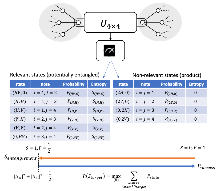
To summarize, when measuring the qubits $(c,d)$, there are several possible final states that can be obtained with certain probabilities, and associated entanglement entropies (45), defined by the Von Neumann entropy of the reduced density matrix after tracing out $f_{3}$,$f_{4}$ from (24). Since there are several possible final states, there are various ways to define the entanglement entropy of the type II fusion process, such as the mean entanglement entropy. We will consider the following question: Given an entanglement entropy $S$, what is the highest probability to obtain a state, whose entanglement entropy is at least $S$. We will refer to such $S$, as the target entropy of the fusion.

Given a target entropy $S_{target}$, we define the probability to reach this target entropy, as the sum of the probabilities over all final states, whose entanglement entropy is at least $S_{target}$. Our goal will be to maximize the probability to reach $S_{target}$ in the fusion process, thus we will calculate:

P​(St​a​r​g​e​t)=max{U}β€‹βˆ‘s​t​a​t​e,Ss​t​a​t​eβ‰₯St​a​r​g​e​tps​t​a​t​e,𝑃subscriptπ‘†π‘‘π‘Žπ‘Ÿπ‘”π‘’π‘‘subscriptπ‘ˆsubscriptπ‘ π‘‘π‘Žπ‘‘π‘’subscriptπ‘†π‘ π‘‘π‘Žπ‘‘π‘’subscriptπ‘†π‘‘π‘Žπ‘Ÿπ‘”π‘’π‘‘subscriptπ‘π‘ π‘‘π‘Žπ‘‘π‘’P(S_{target})=\max_{\{U\}}\sum_{state,\ S_{state}\geq S_{target}}p_{state}\ , (46)

where the maximum is over all the possible fusion matrices $U$ (22).

Figure 9 displays (46): we are given two cluster states that we fuse. In each cluster we choose one qubit, and measure the two qubits. After the measurement, there are ten possible final states, and as we will show, four of them are product states having zero entanglement entropy (non-relevant states), while the other six states are potentially entangled states (relevant states). For each final state we calculate the probability to obtain it and its entanglement entropy, and evaluate the probability of the target entropy $P(S_{target})$. By optimization over $U$ we find 46. By decreasing of the target entanglement entropy, we increase the probability and vice versa, as shown by the orange and blue arrows.

In the following two sections we will prove analytically that $P(1)=\frac{1}{2}$, and this is satisfied for $U$ iff $|U_{1i}|^{2}+|U_{2i}|^{2}=1$ for every $i$. Also, $P(0)=1$ meaning that if $S_{target}>0$ then $P(S_{target})<1$, as featured also in Figure 9. Then, in section VI we plot numerically the graph of $P(S)$, as derived by numerical optimization. In table 2 in section E in the appendix, we summarize the calculations and results of this section and the next one that do not appear in Figure 9.

IV.1 Notations

For simplicity, we will denote in the following the measurement channels $c_{H},c_{V},d_{H},d_{V}$ by the indices $1,2,3,4$, respectively. Referring to the $i,j$ state will mean referring to the state outcome, after measuring a single photon in each of the $i,j$ states (if $i=j$ then we measure two photons in $i$ state). For instance, the state $(1,2)$ is the state that we obtain after measuring one photon in $c_{H}$ and one photon in $c_{V}$. We define the variables:

$$\displaystyle m_{i}=|U_{1i}|^{2}+|U_{2i}|^{2}\hskip 28.45274ptn_{i}=\frac{1}{2}-m_{i}$$
$$\displaystyle t_{i}=U_{1i}U_{2i}^{*}\hskip 28.45274ptk_{i}=|U_{1i}|^{2}-|U_{2i}|^{2}\ .$$ (47)

Note, that since U is unitary, one has the following relations (see proof A.5 in proofs appendix for the full derivation):

$$\displaystyle m_{1}+m_{2}+m_{3}+m_{4}=2$$
$$\displaystyle n_{1}+n_{2}+n_{3}+n_{4}=0$$
$$\displaystyle t_{1}+t_{2}+t_{3}+t_{4}=0$$
$$\displaystyle k_{1}+k_{2}+k_{3}+k_{4}=0\ .$$ (48)

IV.2 The Wave Function

After measuring (11) is the basis of $(c,d)$, we get a new wave function of the joined of two clusters (26).

Lemma 3.

The wave function (26) after measurement (11) is as follows:
(i) The wave function of the state $(i,i)$ reads:

$$\displaystyle\ket{\phi}_{ii}=\frac{1}{N_{ii}}(U_{1i}U_{3i}f_{1}f_{3}+U_{1i}U_{4i}f_{1}f_{4}$$
$$\displaystyle+U_{2i}U_{3i}f_{2}f_{3}+U_{2i}U_{4i}f_{2}f_{4})$$
$$\displaystyle=\frac{1}{N_{ii}}(U_{1i}f_{1}+U_{2i}f_{2})(U_{3i}f_{3}+U_{4i}f_{4})\ ,$$ (49)

where $N_{ii}$ is the normalization factor.
(ii) The wave function of the state (i,j) with iβ‰ j𝑖𝑗i\neq j reads:

$$\ket{\phi}_{ij}=\frac{1}{N_{ij}}(a_{ij}f_{1}f_{3}+b_{ij}f_{1}f_{4}+c_{ij}f_{2}f_{3}+d_{ij}f_{2}f_{4})\ ,$$ (50)

where the coefficients are:

$$\displaystyle a_{ij}=U_{1i}U_{3j}+U_{1j}U_{3i}\hskip 14.22636ptb_{ij}=U_{1i}U_{4j}+U_{1j}U_{4i}$$
$$\displaystyle c_{ij}=U_{2i}U_{3j}+U_{2j}U_{3i}\hskip 14.22636ptd_{ij}=U_{2i}U_{4j}+U_{2j}U_{4i}$$
$$\displaystyle N_{ij}=\sqrt{|a_{ij}|^{2}+|b_{ij}|^{2}+|c_{ij}|^{2}+|d_{ij}|^{2}}=\sqrt{4p_{ij}}\ ,$$ (51)

and $p_{ij}$ is the probability to get the state $(i,j)$ which will be discussed in the next subsection.

Proof.

This is proven in proofs appendix, proof A.6. ∎

From equation (49) one concludes that $(i,i)$ is a product state. We will refer to these product states as irrelevant states, and will refer to the iβ‰ j𝑖𝑗i\neq j states as relevant states, since they are potentially entangled.

Remark 8.

For a relevant state, if two of the four elements $U_{1i},U_{2i},U_{1j},U_{2j}$ are zero, then its is a product state, except for the cases $U_{1i}=U_{2j}=0$ or $U_{1j}=U_{2i}=0$.

IV.3 The States Probabilities

Lemma 4.

The probabilities to reach any of the states are as follows:
(i) The probability to obtain the relevant state $(i,j)$ (iβ‰ j𝑖𝑗i\neq j) is:

$$\displaystyle p_{ij}=\frac{1}{4}(m_{i}(1-m_{j})+m_{j}(1-m_{i}))$$
$$\displaystyle-\frac{1}{2}|U_{1i}U_{1j}^{*}+U_{2i}U_{2j}^{*}|^{2}$$
$$\displaystyle=\frac{1}{8}-\frac{1}{2}n_{i}n_{j}-\frac{1}{2}|U_{1i}U_{1j}^{*}+U_{2i}U_{2j}^{*}|^{2}\leq\frac{1}{4}\ .$$ (52)

(ii) The probability to obtain the non-relevant state $(i,i)$ is:

$$\displaystyle p_{ii}=\frac{1}{2}m_{i}(1-m_{i})=\frac{1}{8}-\frac{1}{2}n_{i}^{2}\ .$$ (53)
Proof.

This is proven in proofs appendix, proof A.7. ∎

Summing over $i$ in equation (53), we get that the probability of obtaining one of the non-relevant states is:

$$\displaystyle p_{non-relevant}=\frac{1}{2}(1-n_{1}^{2}-n_{2}^{2}-n_{3}^{2}-n_{4}^{2})\leq\frac{1}{2}\ .$$ (54)

IV.4 Reduced Density Matrix and Entanglement Entropy

The reduced density matrix (obtained from tracing out $f_{3}$,$f_{4}$ from $\rho_{ij}=\ket{\phi}_{ij}\bra{\phi}_{ij}$) is:

$$\rho_{ij}=\frac{1}{N_{ij}^{2}}\left(\begin{bmatrix}|a_{ij}|^{2}+|b_{ij}|^{2}&a_{ij}^{*}c_{ij}+b_{ij}^{*}d_{ij}\\ a_{ij}c_{ij}^{*}+b_{ij}d_{ij}^{*}&|c_{ij}|^{2}+|d_{ij}|^{2}\end{bmatrix}\right)\ .$$ (55)

Denote by $\lambda_{ij}$, $1-\lambda_{ij}$ the eigenvalues of $\rho_{ij}$, then the Von Neumann entropy reads:

$$\displaystyle S_{ij}=-\lambda_{ij}\log_{2}\lambda_{ij}-(1-\lambda_{ij})\log_{2}{(1-\lambda_{ij})}\ .$$ (56)

The entropy increases monotonically for $\lambda\in[0,\frac{1}{2}]$ and the maximally entanglement entropy state is at $\lambda=\frac{1}{2}$. It will be useful to work with the determinant that shares the same monotonicity property:

$$\displaystyle det(\rho_{ij})=\lambda_{ij}(1-\lambda_{ij})\ .$$ (57)
Lemma 5.

The determinant satisfies:

$$\displaystyle det(\rho_{ij})=\frac{|a_{ij}d_{ij}-b_{ij}c_{ij}|^{2}}{N_{ij}^{4}}$$
$$\displaystyle=\left|\frac{(U_{1i}U_{2j}-U_{1j}U_{2i})(U_{3j}U_{4i}-U_{3i}U_{4j})}{4p_{ij}}\right|^{2}\ .$$ (58)
Proof.

See details of the computation in A.8 in the proofs appendix. ∎

We will mostly work with the determinant since it is easy to calculate. The entanglement entropy (56) can be calculated using:

$$\displaystyle\lambda_{ij}=\frac{1+\sqrt{1-4\det(\rho_{ij})}}{2}$$
$$\displaystyle 1-\lambda_{ij}=\frac{1-\sqrt{1-4\det(\rho_{ij})}}{2}\ .$$ (59)
Remark 9.

One can deduce from (58) that the relevant state $(i,j)$ is a product state iff $U_{1i}U_{2j}=U_{2i}U_{1j}$ or $U_{3j}U_{4i}=U_{3i}U_{4j}$.

In relation to the sets of final states that we discussed in section III as summarized in table 1, the determinant shows that any final state that is a stabilizer state (satisfying the conditions of Theorem 1), or a cluster state up to one-qubit or two-qubit gate operations (satisfying the conditions of Theorem 3), is a maximal entanglement entropy state. A final state that is a Weighted graph state (satisfying the conditions of Theorem 2) is not necessarily a maximal entanglement entropy state. If $|n(b)|=2$ then by theorem 2 it is a stabilizer state, thus a maximally entangled state. However, if $|n(b)|=1$, then we can represent $a,b,c,d$ in the parametrization (34) (for which $N=1$), and by plugging it in (58) we get the determinant:

$$\displaystyle det(\rho)=\frac{\cos^{2}(\phi_{1}-\phi_{2})}{4}=\frac{1-\cos{\chi}}{8}\ ,$$ (60)

where we substitute $\chi$ (33) from (35). The appropriate eigenvalues (59) are $\frac{1\pm\absolutevalue{\cos{\frac{\chi}{2}}}}{2}$, from which one can compute the entropy (56). This is not necessarily a maximally entangled state, as will be shown in the following theorem.

Theorem 4 (Maximally entangled Weighted graph states).

If $|n(b)|=1$, then a Weighted graph state is maximally entangled iff it is a cluster state up to one-qubit gates.

Final State Det / Entropy
General Final State (26) $0\leq S\leq 1\hskip 35.56593pt$ $0\leq det\rho\leq\frac{1}{4}$
Required Final Cluster State $S=1$ (max S)
Stabilizer State (III.2) $S=1$ (max S)
Weighted Graph State (III.3) $\det\rho=\frac{1-\cos\chi}{8}$ (60) (max S iff $\chi=\pi$)
Cluster Up to Two-Qubit Rotations (III.5) $S=1$ (max S)
Table 1: The determinant (57)/entropy (56) of the states, described in section III.
Proof.

The state is maximally entangled iff the determinant in (60) equals $\frac{1}{4}$, which is equivalent to $\phi_{1}=\phi_{2}$, and by Theorem 3 is equivalent to the state being a cluster state up to one-qubit gates.

∎

Remark 10.

The form of the cluster states up to one and two-qubit gates (43) is obtained by substituting $\theta_{b}=\theta_{a}+\frac{\pi}{2}$ and $\theta_{a}=\theta_{1},\theta_{d}=\theta_{2}$ in the general form of two-qubit maximally entangled states:

$$\displaystyle A=\frac{1}{\sqrt{2}}e^{i\theta_{a}}\cos{\phi}\hskip 14.22636ptB=\frac{1}{\sqrt{2}}e^{i\theta_{b}}\sin{\phi}$$
$$\displaystyle C=\frac{1}{\sqrt{2}}e^{i(\theta_{a}+\theta_{d}-\theta_{b})}\sin{\phi}\hskip 14.22636ptD=-\frac{1}{\sqrt{2}}e^{i\theta_{d}}\cos{\phi}\ .$$ (61)

The form (61) is shown in proof A.9.

V An Analytical Probability Bound

Our goal in theorems 5 and 6 is to show that the highest probability to obtain a maximally entanglement entropy state is $\frac{1}{2}$, and to identify all the unitary matrices $U$ that yield this probability. Our proof will be more general than the proof in MaxEfficiency , since we will allow any final maximally entangled state and not only one of the four bell states (up to global phase) as in MaxEfficiency . This is important because we showed in Theorems 1 and 3 that there are final states other than the four Bell states from which one can construct the required cluster state. Unlike the proof in MaxEfficiency we will not allow vacuum modes, i.e. no transformation from the qubits $a,b$ to a general n-qubit set $c_{1},c_{2},...,c_{n}$ with $n>2$, which are all being measured. In theorem 8 we will prove that one cannot obtain a nonzero entanglement entropy with probability one. Thus, we will characterize the two edges of the graph of $P(S)$, as illustrated in Figure 9.

Theorem 5 (The probability to obtain a maximally entanglement state bounded by $\frac{1}{2}$).

For every matrix $U$, when measuring $c$ and $d$, the probability to obtain a maximally entanglement entropy state is bounded from above by $\frac{1}{2}$.

Proof.

This theorem is proved using the following Lemmas.

Lemma 6.

The conditions for a relevant $(i,j)$ state to be a maximally entanglement entropy state are:

$$\displaystyle n_{i}t_{j}+n_{j}t_{i}=0\ ,$$ (62)

and

$$\displaystyle n_{i}k_{j}+n_{j}k_{i}=0\ .$$ (63)
Proof.

The reduced density matrix $\rho_{ij}$ (55) of a maximally entanglement entropy relevant state $(i,j)$ is $\frac{1}{2}Id_{2\times 2}$. Thus, the off diagonal elements of $\rho_{ij}$ and difference between the two diagonal elements are 00. We impose these two conditions, with a multiplication by $N_{ij}^{2}$. The first condition reads:

$$\displaystyle 0=a_{ij}c_{ij}^{*}+b_{ij}d_{ij}^{*}=2t_{i}n_{j}+2t_{j}n_{i}\ ,$$ (64)

(see details of computation in proof A.10 in proof appendix) and the second condition reads:

$\displaystyle 0=|a_{ij}|^{2}+|b_{ij}|^{2}-|c_{ij}|^{2}-|d_{ij}|^{2}$
$\displaystyle=4n_{i}|U_{1j}|^{2}+4n_{j}|U_{1i}|^{2}+4n_{i}n_{j}-n_{i}-n_{j}$
$\displaystyle=2n_{i}k_{j}+2n_{j}k_{i}\ ,$ (65)

(see details of computation in proof A.11 in proof appendix). ∎

Lemma 7.

If $(i,j)$ is a relevant maximally entanglement entropy state, then the probability to obtain it is bounded from above by $\frac{1}{8}$. If the bound is saturated then $n_{i}=n_{j}=0$.

Proof.

See proof A.12 in proof appendix. ∎

Lemma 8.

When all the relevant states are maximally entanglement entropy states then $n_{1}=n_{2}=n_{3}=n_{4}=0$, and the probability to obtain a maximally entanglement entropy state is $\frac{1}{2}$.

Proof.

When all the relevant states are maximally entanglement entropy states, then from (62) one gets that either all $n$’s or all $t$’s are zero (for details see proof A.13 in proof appendix). If all the $t$’s vanish, then for every $i$, one of $U_{1i}$,$U_{2i}$ is zero. Thus, we can choose two indices $(i,j)$ for which either $U_{1i}=U_{2i}=0$ or $U_{2i}=U_{2j}=0$, and the state $(i,j)$ is a product state (see Remark 8), hence a contradiction. Therefore, all the $n$’s are zero. In this case, the probability for non-relevant states (54) is $\frac{1}{2}$, which is also the probability for all the relevant states. When $n_{i}=n_{j}=0$ then by Lemma 6 the two conditions (62),(63) for $(i,j)$ state to be a maximally entanglement entropy state are fulfilled, hence, in this case all the relevant states are maximally entanglement entropy states and we have $\frac{1}{2}$ probability to get a maximally entanglement entropy state. ∎

Lemma 9.

There cannot be exactly five relevant states that are maximally entanglement entropy states, except when all the $n$’s are zero.

Proof.

See proof A.14 in proof appendix. ∎

Now, we can complete the proof: If we have four maximally entanglement entropy states or less, then the probability to get a maximally entanglement entropy state is bounded from above by $4\times\frac{1}{8}=\frac{1}{2}$ by Lemma 7. Else, by Lemma 9 we have six maximally entanglement entropy states, and by Lemma 8 the probability is $\frac{1}{2}$.

∎

Theorem 6 (Saturating the $P=\frac{1}{2}$ bound).

The set of matrices $U$ which lead to a saturation of the $\frac{1}{2}$ bound, is the set of all the matrices for which all the $n$’s (47) are zero, that is the matrices $U$ that satisfy:

$$|U_{1i}|^{2}+|U_{2i}|^{2}=\frac{1}{2},\leavevmode\nobreak\ \leavevmode\nobreak\ \leavevmode\nobreak\ i=1,2,3,4\ .$$ (66)
Proof.

If all the six states are maximally entanglement entropy state, then we have already shown that all the n’s are zero. We also showed, that the number of maximally entanglement entropy states cannot be five by Lemma 9, thus we are left with the case that there are four maximally entanglement entropy states or less. If a relevant state is maximally entanglement entropy state then by Lemma 7 the probability to obtain this state is bounded from above by $\frac{1}{8}$, so, if we have four states or less, then the only option to get to a total probability $P=\frac{1}{2}$ is if to have exactly four maximally entanglement entropy states, with probability $\frac{1}{8}$ for each one. By Lemma 7, we have $n_{i}=n_{j}=0$ for every $(i,j)$ of the four states.

Lemma 10.

If there are four different subsets of the set $\{1,2,3,4\}$, each one consisting of two elements, then one can choose two of the subsets such that their union is the set $\{1,2,3,4\}$ Β .

Proof.

see proof A.15 in proofs appendix. ∎

By Lemma 10 one can choose two of the four states, $(i,j)$ and $(k,l)$ such that $\{i,j,k,l\}=\{1,2,3,4\}$. Hence, $n_{i}=n_{j}=n_{k}=n_{l}=0$, thus all the $n$’s are zero and we are done.

∎

Theorem 7 (Minimal number of single-qubit gates).

The minimal number of single-qubit linear optical devices, that are needed to construct the matrix $U$ that saturates the $P=\frac{1}{2}$ bound is two.

Proof.

If one use only one single-qubit gate, then in the matrix $U$ there will be two rows, that are the same as in the identity matrix, thus it will not obey the condition (66). One can use two gates to construct a matrix, $U$ that will obey (66). For instance, a $45$ degrees rotation for $a_{H},b_{H}$ and a $45$ rotation for $a_{V},b_{V}$:

$$\displaystyle U=\begin{bmatrix}\frac{1}{\sqrt{2}}&0&\frac{1}{\sqrt{2}}&0\\ 0&1&0&0\\ -\frac{1}{\sqrt{2}}&0&\frac{1}{\sqrt{2}}&0\\ 0&0&0&1\end{bmatrix}\begin{bmatrix}1&0&0&0\\ 0&\frac{1}{\sqrt{2}}&0&\frac{1}{\sqrt{2}}\\ 0&0&1&0\\ 0&-\frac{1}{\sqrt{2}}&0&\frac{1}{\sqrt{2}}\end{bmatrix}$$
$$\displaystyle=\frac{1}{\sqrt{2}}\begin{bmatrix}1&0&1&0\\ 0&1&0&1\\ -1&0&1&0\\ 0&-1&0&1\end{bmatrix}\ ,$$ (67)

and this matrix indeed obeys (66).

∎

If the fusion of (67) succeeds, then the fusion operator is $\bra{0}_{a}\bra{1}_{a}\pm\bra{0}_{a}\bra{1}_{a}$ and one arrives at the same situation as in (20). This is a projection to one of the Bell states that yields the required cluster state.

It is important to note that two optical devices is less than the three, that are being used in the construction of the regular type II fusion as in (23).

Theorem 8 (Probability $P(S)=1$ iff $S=0$).

The success probability is one iff the target entropy is zero, i.e. the final state (26) is a product state.

Proof.

Assume that there is $P(S)=1$ probability of success to obtain a final state with nonzero entropy $S$ or higher. Then, the probability for all the non-relevant states (54) must be zero, and from equations (48) and (54) one concludes that two of the $n$’s are $\frac{1}{2}$ and the other two are $-\frac{1}{2}$. When $n_{i}=-\frac{1}{2}$ then $m_{i}=0$ so $U_{1i}=U_{2i}=0$, hence from remark 8 every $(i,j)$ state (50) is a product state, for every $j$. Thus, one has five relevant states, that are product states, and the sixth state has $n_{i}=n_{j}=0.5$, hence, its probability is zero (by equation 52). Therefore, one gets a $P=1$ probability to obtain product state and $S=0$. ∎

VI Numerical Simulations

In order to quantitatively evaluate (46), and to validate our analytical analysis we construct a simulator using the PyTorch package, Python and optimize general $4\times 4$ unitary matrices $U$ (22), which we parameterize by Euler angles SUN ; AnotherSUN . To improve the convergence rate, we initialized the optimization parameters after taking the best result among randomly-sampled matrices, which we sample using the Haar probability measure (for details see appendix C). In subsection VI.1 we will present and discuss the results of the optimization of the expectation value of the entanglement entropy, and in subsection VI.2, the optimization of the minimal entanglement entropy.

VI.1 Optimization of the Mean Entanglement Entropy

Define the expectation value of the entanglement entropy of the final states as

⟨S⟩=βˆ‘(i,j)​s​t​a​t​epi​j​Si​j,delimited-βŸ¨βŸ©π‘†subscriptπ‘–π‘—π‘ π‘‘π‘Žπ‘‘π‘’subscript𝑝𝑖𝑗subscript𝑆𝑖𝑗\langle S\rangle=\sum_{(i,j)state}p_{ij}S_{ij}\ , (68)

where the summation is over all the final states $(i,j)$ (50), $p_{ij}$ (52) is the probability to obtain the state $(i,j)$, and $S_{ij}$ is its entanglement entropy (56). Since all the non-relevant (49) states are product states having zero entropy, one can replace the summation by a sum (68) over the relevant states. Define the total probability $p_{total}\equiv p_{relevant}=1-p_{non-relevant}$ to be the sum of the probabilities of all the relevant states, which is (by (54)):

$$\displaystyle p_{total}=\frac{1}{2}(1+n_{1}^{2}+n_{2}^{2}+n_{3}^{2}+n_{4}^{2})\ .$$ (69)

The goal is, given a target total probability $p$, to maximize the expectation value of the entropy

$$\displaystyle\langle S\rangle_{max}(p)\equiv\max_{\{U|p_{total}(U)=p\}}\langle S\rangle\ .$$ (70)

We randomly sample matrices, locate them in the $S-P$ plane, and calculate the mean and the standard deviation of the expectation value of the entanglement entropy for each probability sum. These are the gray shaded area, and the green line, respectively, in Figure 10). Using the optimization scheme, we sweep over all the probabilities between $0.5$ and $1.0$, (in steps of 0.01), and for each point we optimize the target probability and maximal expectation value of the entropy. We will refer in the following to the expectation value of the entropy and the expectation entropy. We average the results over 20 runs, while we initialize the optimization to be one of the highest expectation entropy among those found in the random steps. Each run is optimized to find a specific target probability and a maximal expectation entropy. The cost function for the optimization reads:

$$\displaystyle\mathcal{L}_{expectaion}\equiv\alpha\left||p\left(U\right)-p_{target}|\right|^{2}-\langle S\rangle_{max}\left(U\right)\ .$$ (71)

In practice, we add baseline to the cost function in order to avoid negative values (for numerical stability in the gradient descent). $\alpha$ is a hyperparameter which we tuned, and pracitcally set it to 1. We use Adam Optimizer for $1,000$ epochs, with a learning rate of $0.001$. The results are shown in Figure 10 in the red line.

Refer to caption
Figure 10: Plot of the expectation value of the entanglement entropy (expectation entropy) versus the total success probability. The gray area is created by randomly sampling matrices. The green line represents the average expectation entropy for each total probability (plus or minus the standard deviation in the dashed line). The red line shows the maximal (red) expectation value of entropy versus the probability, after using an optimization scheme.

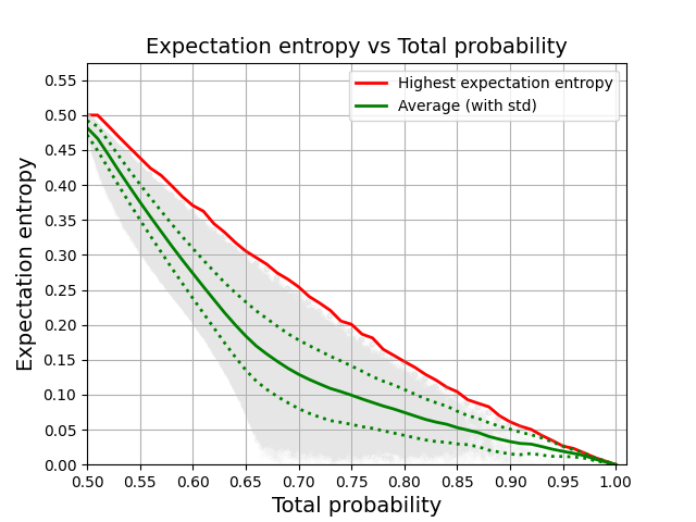
Note, that the relation between the expectation entropy and the total probability is monotonically decreasing (as can be seen in the graph), namely, during the optimization process, increasing the expectation entropy leads to a decrease in the total probability. Therefore, there is a small bias of the optimization results towards lower probability. The graph exhibits an intriguing close to linear structure :

$$\displaystyle S=1-P\ ,$$ (72)

for which we lack an analytical derivation. The plot reveals a critical probability, around $\frac{2}{3}$, where for any probability below it there is at least one relevant state that is not separable, since the average entropy is always greater than zero in this range.

The range of values of the expectation entropy is the interval $[0,1]$. When the total probability is $0.5$, then all the relevant states are maximally entanglement entropy states, as we proved in Theorem 6, and the expectation entropy is equal to $0.5\cdot 1=0.5$. When the total probability is $1$, then as shown in theorem 8, all the relevant states are product states, with entropy zero, and the expectation entropy is therefor equal to zero. Note, also that the variance of the expectation entropy is relatively small near the $0.5$ and $1$, and increases in between. This implies that choosing a random fusion unitary operation is not the right strategy, when attempting to have a high probability for the fusion success, while reducing the entanglement entropy of the fusion link.

VI.2 Optimization of the Minimal Entanglement Entropy

Our aim is to maximize the probability to reach $S_{target}$ in the fusion process (46), by optimizing the matrix $U$. The cost function for the optimization is:

$$\displaystyle\mathcal{L}\equiv-P(S_{target})\ ,$$ (73)

and the results are shown in Figure 11. The number of states $n_{i}$, whose entropy is not lower than the given minimal entropy $n_{i}$, is shown in Figure 12.

Refer to caption
Figure 11: The probability for the success of the fusion process versus the minimal entropy, according to definition 46. The gray area is constructed by randomly sampling matrices. The red line shows the maximal probability for each minimal entropy, as is obtained by the optimization. The horizontal axis is in units of $\log_{2}{e}$
Refer to caption
Figure 12: Number of states ($n_{i}$) for each of the points in Figure 11 (the gray points match, as well as the red points). The vertical axis represents the number of states among the six states, and the horizontal axis represents the minimal entropy. The horizontal axis is in units of $\log_{2}{e}$. It is clear from this graph that the optimal matrices employ all the six states.

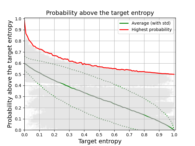
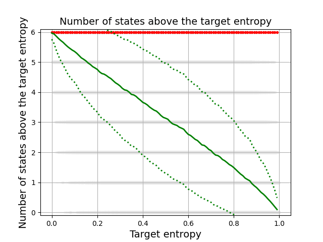
Figure 11 shows, as expected, a monotonically decreasing graph. The graph is convex, the decrease is faster in the left regime, and slows down with the increase of the minimal entropy. In the right regime, the graph is nearly flat. Thus, the numerical data suggests that the left regime is relevant for decreasing the target entropy and getting a higher probability of success. On the other hand, in the right regime, it is useful to increase the target entropy to one, since it lowers only slightly the probability of success. The number of states that are being used in the optimal matrix is fixed at six, which means that all the relevant states contribute for the optimal solutions fro any target entropy. Therefore, the y-axis corresponding to the red line $p(S)$ in Figure 11 is $p_{relevant}=\frac{1}{2}(1+n_{1}^{2}+n_{2}^{2}+n_{3}^{2}+n_{4}^{2})$. This, however, does not mean that there are no optimal solutions with less than six states, e.g. one can have solutions with four states, with the other two relevant states having a zero success probability. Inspecting the mean $p(S)$ (before optimization) and the distribution in Figure 11, reveals a large distance between the mean and the maximal values, which emphasizes the significance of finding the optimal $U$’s, rather than having a random one. One also sees in Figure 12, that the average number of states $n_{i}$, that are being used, is decreasing, as expected.

Acknowledgements We would like to thank I. Kaplan for participation in the early stages of this project, M. Erew for a valuable discussion and Ori Shem-Ur for comments on the manuscript. This work is supported in part by the Israeli Science Foundation Excellence Center, the US-Israel Binational Science Foundation, and the Israel Ministry of Science.

VII Discussion and Outlook

We generalized the type II fusion procedure, and analyzed it both analytically and numerically. We classified all the possible final states of the generalized type II fusion, including the probability for the success of the fusion, and its correlation with the entanglement entropy of the fusion link. In addition to having as final states the cluster states, where the entanglement entropy of the fusion link is maximal, we considered Weighted graph states that furnish fusion links, whose entanglement entropy is not maximal, while having a higher success probability for the fusion.

This raises a natural question, whether such Weighted graph states can be utilized as resource states for quantum computation, or for other tasks gross2007measurement . It is also worth analysing the role that such states may play, when adding ancilla qubits to the fusion process. We found, that allowing maximally entangled states, which are not Bell states, as final states, does not increase the probability of the fusion success above the fifty percent bound, if no ancilla qubits are used. It would be important to find, whether this changes with the addition of ancilla qubits.

Analytically, we proved in a rather general setup, the fifty percent bound on the fusion probability success, and classified the fusion matrices and the set of final states, which is larger than the set that has been previously considered. We proved, that only fusion links with zero entanglement entropy can be constructed with a hundred percent probability of success. We have not obtained, however, an analytical formula for the fusion probability success $p(S)$ for a general entanglement entropy $S$ of the fusion link, and we analyzed it numerically. It would be interesting to further explore this analytically.

Another route to take is to generalize the analysis to the cases, where one allows a unitary operation that involves more registers as in MaxEfficiency . Since MBQC can be defined on resource states made of qudits, it is natural to generalize our work to such cases. Finally, it would be interesting to have experimental realizations of the various resource states that we studied.

References

  • (1) R.Β Raussendorf and H.Β Briegel. Computational model underlying the one-way quantum computer. Arxiv, 2002. https://arxiv.org/abs/quant-ph/0108067.
  • (2) H.Β J. Briegel, D.Β E. Browne, W.Β DΓΌr, R.Β Raussendorf, and M.Β VanΒ den Nest. Measurement-based quantum computation. Arxiv, 2009. https://arxiv.org/abs/0910.1116.
  • (3) R.Β Raussendorf, D.Β E. Browne, and H.Β J. Briegel. Measurement-based quantum computation with cluster states. Arxiv, 2003. https://arxiv.org/abs/quant-ph/0301052.
  • (4) SwapnilΒ Nitin Shah. Realizations of measurement based quantum computing. Arxiv, 2021. https://arxiv.org/abs/2112.11601.
  • (5) M.Β A. Nielsen. Cluster-state quantum computation. ArXiv, 2005. https://doi.org/10.1016/S0034-4877(06)80014-5.
  • (6) H.Β J. Briegel and R.Β Raussendorf. Persistent entanglement in arrays of interacting particle s. Arxiv, 2000. https://arxiv.org/abs/quant-ph/0004051.
  • (7) P.Β Walther, K.Β J. Resch, T.Β Rudolph, E.Β Schenck, H.Β Weinfurter, V.Β Vedral, M.Β Aspelmeyer, and A.Β Zeilinger. Experimental one-way quantum computing. Arxiv, 2005. https://arxiv.org/abs/quant-ph/0503126.
  • (8) Kai Chen, Che-Ming Li, Qiang Zhang, Yu-Ao Chen, Alexander Goebel, Shuai Chen, Alois Mair, and Jian-Wei Pan. Experimental realization of one-way quantum computing with two-photon four-qubit cluster states. Arxiv, 2007. https://arxiv.org/abs/0705.0174.
  • (9) Giuseppe Vallone, Enrico Pomarico, FrancescoΒ De Martini, and Paolo Mataloni. Active one-way quantum computation with 2-photon 4-qubit cluster states. Arxiv, 2007. https://arxiv.org/abs/0712.1889.
  • (10) M.Β S. Tame, B.Β A. Bell, C.Β DiΒ Franco, W.Β J. Wadsworth, and J.Β G. Rarity. Experimental realization of a one-way quantum computer algorithm solving simon’s problem. Arxiv, 2014. https://arxiv.org/abs/1410.3859.
  • (11) E.Β Knill, R.Β Laflamme, and G.Β Milburn. A scheme for efficient quantum computation with linear optics. Nature, 2001. https://www.nature.com/articles/35051009.
  • (12) E.Β Knill, R.Β Laflamme, and G.Β Milburn. Efficient linear optics quantum computation. Arxiv, 2000. https://arxiv.org/abs/quant-ph/0006088.
  • (13) M.Β A. Nielsen. Optical quantum computation using cluster states. Arxiv, 2004. https://arxiv.org/abs/quant-ph/0402005.
  • (14) N.Β Yoran and B.Β Reznik. Deterministic linear optics quantum computation utilizing linked photon circuits. Arxiv, 2003. https://arxiv.org/pdf/quant-ph/0303008.pdf.
  • (15) D.Β E. Browne and T.Β Rudolph. Resource-efficient linear optical quantum computation. ArXiv, 2004. https://doi.org/10.1103/PhysRevLett.95.010501.
  • (16) S.Β Bartolucci, P.Β Birchall, H.Β BombΓ­n, H.Β Cable, C.Β Dawson, M.Β Gimeno-Segovia, E.Β Johnston, K.Β Kieling, N.Β Nickerson, M.Β Pant, F.Β Pastawski, T.Β Rudolph, and C.Β Sparrow. Fusion-based quantum computation. 2021. https://arxiv.org/pdf/2101.09310.pdf.
  • (17) M.Β Gimeno-Segovia, P.Β Shadbolt, D.Β E. Browne, and T.Β Rudolph. From three-photon ghz states to ballistic universal quantum computation. 2015. https://arxiv.org/pdf/1410.3720.pdf.
  • (18) J.Β Calsamiglia and N.Β LΓΌtkenhaus. Maximum efficiency of a linear-optical bell-state analyzer. 2001.
  • (19) N.Β LΓΌtkenhaus, J.Β Calsamiglia, and K-A. Suominen. On bell measurements for teleportation. 1999. https://arxiv.org/pdf/quant-ph/9809063.pdf.
  • (20) W.Β P. Grice. Arbitrarily complete bell-state measurement using only linear optical elements. Physical Review A, 2011. https://journals.aps.org/pra/abstract/10.1103/PhysRevA.84.042331.
  • (21) F.Β Ewert and P.Β V. Loock. 3/4-efficient bell measurement with passive linear optics and unentangled ancillae. Arxiv, 2014. https://arxiv.org/abs/1403.4841.
  • (22) T.Β Kilmer and S.Β Guha. Boosting linear-optical bell measurement success probability with pre-detection squeezing and imperfect photon-number-resolving detectors. Arvix, 2018. https://arxiv.org/abs/1809.09264.
  • (23) M.Β J. Bayerbach, S.Β E. D’Aurelio, P.Β V. Loock, and S.Β Barz. Bell-state measurement exceeding 50optics. Arxiv, 2022. https://arxiv.org/abs/2208.02271.
  • (24) P.Β Kok, W.Β J. Munro, K.Β Nemoto, T.Β C. Ralph, J.Β P. Dowling, and G.Β J. Milburn. Linear optical quantum computing. Arxiv, 2006. https://arxiv.org/abs/quant-ph/0512071.
  • (25) T.Β C. Ralph and G.Β J. Pryde. Optical quantum computation. Arxiv, 2011. https://arxiv.org/abs/1103.6071.
  • (26) Pieter Kok. Five lectures on optical quantum computing. arXiv: Quantum Physics, 787:187–219, 2007.
  • (27) M.Β Hein, W.Β Dur, J.Β Eisert, R.Β Raussendorf, M.Β V.Β D. Nest, and H.Β J. Briegel. Entanglement in graph states and its applications. Arxiv, 2006. https://arxiv.org/abs/quant-ph/0602096.
  • (28) DouglasΒ Brent West etΒ al. Introduction to graph theory. Prentice hall Upper Saddle River, 2001.
  • (29) Marc Hein, Jens Eisert, and HansΒ J Briegel. Multiparty entanglement in graph states. Physical Review A, 69(6):062311, 2004.
  • (30) WΒ DΓΌr, LΒ Hartmann, MΒ Hein, MΒ Lewenstein, and H-J Briegel. Entanglement in spin chains and lattices with long-range ising-type interactions. Physical review letters, 94(9):097203, 2005.
  • (31) C.Β Adami and N.Β J. Cerf. Quantum computation with linear optics. Arxiv, 1998. https://arxiv.org/abs/quant-ph/9806048.
  • (32) H.Β J. Bernstein and P.Β Bertani. Experimental realization of any discrete unitary operator. Arxiv, 1994. https://journals.aps.org/prl/abstract/10.1103/PhysRevLett.73.58.
  • (33) H.Β deΒ Guise, B.Β C. Sanders, S.Β D. Bartlett, and W.Β Zhang. Geometric phase in su(n) interferometry. Arxiv, 2001. https://arxiv.org/abs/quant-ph/0104106.
  • (34) I.Β Dhand and S.Β K. Goyal. Realization of arbitrary discrete unitary transformations using spatial and internal modes of light. Arxiv, 2015. https://arxiv.org/abs/1508.06259.
  • (35) Karol Zyczkowski and Ingemar Bengtsson. An introduction to quantum entanglement: a geometric approach. Arxiv, 2006. https://arxiv.org/abs/quant-ph/0606228.
  • (36) T.Β Tilma and E.Β C. Sudarshan. Generalized euler angle parameterization for su(n). ArXiv, 2002. https://arxiv.org/abs/math-ph/0205016.
  • (37) T.Β Tilma, M.Β Byrd, and E.Β C.Β G. Sudarshan. A parametrization of bipartite systems based on su(4) euler angles. ArXiv, 2002. https://iopscience.iop.org/article/10.1088/0305-4470/35/48/315.
  • (38) Daivd Gross, Jens Eisert, Norbert Schuch, and David Perez-Garcia. Measurement-based quantum computation beyond the one-way model. Physical Review A, 76(5):052315, 2007.
  • (39) Stasja Stanisic. Universal quantum computation by linear optics, 2015.
  • (40) E.Β Meckes. The Random Matrix Theory of the Classical Compact Groups. Cambridge University Press, 2019.

Appendix A Detailed Proofs

A.1 Proof of Lemma 1

If $a^{\prime}=e$, then acting on (26) with $\prod_{c\in n(L)\cup n(b)}Z_{c}$ yields the state:

$$\displaystyle A\ket{0}_{e}\prod_{c\in n(L)}Z_{c}\ket{\phi_{L}}_{V_{L}\setminus\{L\}}\prod_{d\in n(b)}Z_{d}\ket{\phi_{b}}_{V_{b}\setminus\{b\}}$$
$$\displaystyle+B\ket{0}_{e}\prod_{c\in n(L)}Z_{c}\ket{\phi_{L}}_{V_{L}\setminus\{L\}}\ket{\phi_{b}}_{V_{b}\setminus\{b\}}$$
$$\displaystyle+C\ket{1}_{e}\ket{\phi_{L}}_{V_{L}\setminus\{L\}}\prod_{d\in n(b)}Z_{d}\ket{\phi_{b}}_{V_{b}\setminus\{b\}}$$
$$\displaystyle+D\ket{1}_{e}\ket{\phi_{L}}_{V_{L}\setminus\{L\}}\ket{\phi_{b}}_{V_{b}\setminus\{b\}}\ .$$ (74)

In order to be able to have an hermitian (since it commutes with all the $Z_{c}$ operators and their multiplication should be hermitian) operator, that acts on s​p​a​n​{|0⟩e,|1⟩e}π‘ π‘π‘Žπ‘›subscriptket0𝑒subscriptket1𝑒span\{\ket{0}_{e},\ket{1}_{e}\}, such that the state (74) becomes (26), we have to exchange the $A$ and $D$ terms as well as the $B$ and $C$ terms. Thus, we need to have $AC=BD$, and if this holds then the corresponding operator takes the form $T_{a}=\begin{bmatrix}0&t\\ \frac{1}{t}&0\end{bmatrix}$ when $D=tA$ and $C=tB$, where $t=e^{i\Phi}$ to ensure herimiticity. Hence, we get (28), and therefore the stabilizer (27). Since $t=e^{i\Phi}$ we require $|A|=|D|$, $|B|=|C|$ and $AC=BD$. Note, that in this case, the resulting stabilizer (27) commutes with all the other stabilizers $K_{a^{\prime}}$ when $a^{\prime}$ in neither $e$ nor in $n(b)$. If $a^{\prime}$ in not in $n(L)$ then this is trivial, and if it is, then $Z_{a^{\prime}}$ from $K^{\prime}_{e}$ and $X_{a^{\prime}}$ from $K_{a^{\prime}}$ are anti-commuting, but so do $T_{a}$ from $K^{\prime}_{e}$ and $Z_{e}$ from $K_{a^{\prime}}$.

A.2 Proof of Lemma 2

When $a^{\prime}\in n(b)$, then acting on (26) with the operator $X_{a^{\prime}}\prod_{b^{\prime}\in n(a^{\prime})\setminus\{e\}}Z_{b^{\prime}}$ yields the state:

$$\displaystyle(-1)^{k^{\prime}_{a^{\prime}}}(A\ket{0}_{e}\ket{\phi_{L}}_{V_{L}\setminus\{L\}}\ket{\phi_{b}}_{V_{b}\setminus\{b\}}$$
$$\displaystyle-B\ket{0}_{e}\ket{\phi_{L}}_{V_{L}\setminus\{L\}}\prod_{d\in n(b)}Z_{d}\ket{\phi_{b}}_{V_{b}\setminus\{b\}}$$
$$\displaystyle+C\ket{1}_{e}\prod_{c\in n(L)}Z_{c}\ket{\phi_{L}}_{V_{L}\setminus\{L\}}\ket{\phi_{b}}_{V_{b}\setminus\{b\}}$$
$$\displaystyle-D\ket{1}_{e}\prod_{c\in n(L)}Z_{c}\ket{\phi_{L}}_{V_{L}\setminus\{L\}}\prod_{d\in n(b)}Z_{d}\ket{\phi_{b}}_{V_{b}\setminus\{b\}})\ .$$ (75)

In order to be able to act on s​p​a​n​|0⟩e,|1⟩eπ‘ π‘π‘Žπ‘›subscriptket0𝑒subscriptket1𝑒span{\ket{0}_{e},\ket{1}_{e}} with an operator, such that the state (75) transforms to (26), we need that one of $(A,B)$ to be zero and also one of $(C,D)$. If $A=C=0$ or $B=D=0$, then the state is a product state, so these options are irrelevant, but if $A=D=0$ or $B=C=0$, then acting with $Z_{e}$ yields the required. This yields the regular cluster stabilizer (8) for $a^{\prime}$, which commutes with all the other regular stabilizers, and also with the new stabilizer of $e$ in (27), as follows from the same argument as in proof A.1 in proof appendix.

A.3 Proof of Theorem 2

We begin with the case where $|n(b)|=1$, and let $d$ be the qubit in $n(b)$. Let us put all the qubits in the $\ket{+}$ state, and then act on every connected qubit with $CZ$, except for $d,e$. Thus, we get two clusters - one containing $e$, and the other one containing $d$. The total wave function is:

$$\displaystyle(\ket{0}_{e}\ket{\phi_{L}}_{V_{L}\setminus\{L\}}+\ket{1}_{e}\prod_{c\in n(L)}Z_{c}\ket{\phi_{L}}_{V_{L}\setminus\{L\}})\ket{\phi_{b}}_{V_{b}\setminus\{b\}}\ .$$ (76)

We act with a two-qubit gate on $(d,e)$, and get the state (26). We require this gate to commute with all the $CZ$ gates, this it has to be diagonal in the standard basis $\ket{0},\ket{1}$. This leaves only one option - the operator $T_{e,n(b)}$, defined in (31). In order for this operator to be unitary (up to normalization) we have to require $|A\pm B|=|C\pm D|\in\mathbb{R}$. From this we get:

$$\displaystyle 1=|A|^{2}+|B|^{2}+|C|^{2}+|D|^{2}=$$
$$\displaystyle\frac{1}{2}(|A+B|^{2}+|A-B|^{2}+|C+D|^{2}+|C-D|^{2})$$
$$\displaystyle\Longrightarrow\frac{1}{\sqrt{2}}=|A\pm B|^{2}=|C\pm D|^{2}$$
$$\displaystyle=|A|^{2}+|B|^{2}\pm 2\Re{AB^{*}}=|C|^{2}+|D|^{2}\pm 2\Re{CD^{*}}\ ,$$ (77)

and the conditions in (30) follow.

These conditions can also be written as the parameterization in (34). In this parameterization, the gate $T_{e,n(b)}$ reads:

$$\displaystyle T_{e,n(b)}=e^{i(\theta_{1}+\phi_{1})}\ket{0_{e},0_{d}}\bra{0_{e},0_{e}}+e^{i(\theta_{1}-\phi_{1})}\ket{0_{e},1_{d}}\bra{0_{e},1_{e}}$$
$$\displaystyle+e^{i(\theta_{2}+\phi_{2})}\ket{1_{e},0_{d}}\bra{1_{e},0_{e}}+e^{i(\theta_{2}-\phi_{2}+\pi)}\ket{1_{e},1_{d}}\bra{1_{e},1_{e}}\ .$$ (78)

Denote $\chi_{1,2}=\theta_{1}\pm\phi_{1},\chi_{3}=\theta_{2}+\phi_{2},\chi_{4}=\theta_{2}-\phi_{2}+\pi$. Then, assuming we apply $Z$-rotations and a global phase rotation, we can first perform a global rotation that takes $\chi_{1}$ to zero and all the other $\chi_{i}$ to $\chi_{i}^{\prime}=\chi_{i}-\chi_{1}$. Then, by $Z$-rotations and global phase rotations we act witha phase shift gate on the qubit $e$ with a shift $\chi_{1}-\chi_{3}$, which takes $\chi_{3}^{\prime}$ to $\chi_{3}^{\prime\prime}=\chi_{3}^{\prime}+\chi_{1}-\chi_{3}=0$ and $\chi_{4}^{\prime}$ to $\chi_{4}^{\prime\prime}=\chi_{4}^{\prime}+\chi_{1}-\chi_{3}=\chi_{4}-\chi_{3}$. By the same method we can perfrom a phase shift gate on qubit $d$ with shift $\chi_{1}-\chi_{2}$, which takes $\chi_{2}^{\prime}$ to $\chi_{2}^{\prime\prime}=\chi_{2}^{\prime}+\chi_{1}-\chi_{2}=0$, and we are left with $\chi_{4}^{\prime\prime}=\chi_{4}^{\prime}+\chi_{1}-\chi_{2}=\chi_{1}+\chi_{4}-\chi_{2}-\chi_{3}$. This is the required $\chi$, and by substituting the values of $\chi_{i}$ and peforming modulo $2\pi$, we get (35) as required.

If these conditions are not satisfied, we can still perform a unitary transformation on the qubits $(d,e)$, that takes the state in (76) to the state (26), and in fact there are many such transformations. But, none of those will commute with the $CZ$ gates, so we must use this gate only after all the $CZ$ gates. Consider next the case $|n(b)|=2$ (or greater than 2), and denote by $d_{1},d_{2}$ the qubits in $n(b)$. Assume we again prepared the state in (76) and we wish to get the state (26) by applying 2-qubits gates on the couples $(e,d_{1})$ and $(e,d_{2})$.

In this case, one of $A,B$ has to be zero, because if not, then we must apply on the couple $e,d_{1}$ 2-qubits gate that contains the terms $\ket{0}_{e}\bra{0}_{e}$, $\ket{0}_{e}\bra{0}_{e}Z_{d_{1}}$, which will give us part of the total wave function which is $(A\ket{0}_{e}\ket{\phi_{L}}_{V_{L}\setminus\{L\}}\ket{\phi_{d_{1}}}+B\ket{0}_{e}\ket{\phi_{L}}_{V_{L}\setminus\{L\}}Z_{d_{1}}\ket{\phi_{d_{1}}})\ket{\phi_{d_{2}}}$. Then we need to aplly some 2-qubits gate on $e,d_{2}$ that will contain the terms $\ket{0}_{e}\ket{\phi_{L}}_{V_{L}\setminus\{L\}}\ket{\phi_{d_{1}}}\ket{\phi_{d_{2}}}$ and $\ket{0}_{e}\ket{\phi_{L}}_{V_{L}\setminus\{L\}}Z_{d_{1}}\ket{\phi_{d_{1}}}Z_{d_{2}}\ket{\phi_{d_{2}}}$, but this will also generate the terms $\ket{0}_{e}\ket{\phi_{L}}_{V_{L}\setminus\{L\}}Z_{d_{1}}\ket{\phi_{d_{1}}}\ket{\phi_{d_{2}}}$ and $\ket{0}_{e}\ket{\phi_{L}}_{V_{L}\setminus\{L\}}\ket{\phi_{d_{1}}}Z_{d_{2}}\ket{\phi_{d_{2}}}$ which makes our mission impossible. Following the same argument, one of $C,D$ must be zero. In that case, we can apply the gate in (31) on $e,d_{1}$ and then on $e,d_{2}$ to get the wanted state in (26). If $A=C=0$ or $B=D=0$ then the state is a product state. If $A=D=0$ or $B=C=0$, then from the conditions in (30) it follows that $|A|=|D|$ or $|B|=|C|$, respectively. We, thus, get exactly the conditions of theorem 1 for a stabilizer state.

A.4 Proof of Theorem 3

Back to the more convenient way of the $f$’s, we have $f_{2}=Zf_{1}$ and require $g_{2}=Zg_{1}$, and similarly for $3,4$. We can write the transformation of $f_{1},f_{2}$ as:

$$\displaystyle\begin{bmatrix}g_{1}\\ g_{2}\end{bmatrix}=\begin{bmatrix}T_{11}&T_{12}\\ T_{21}&T_{22}\end{bmatrix}\begin{bmatrix}f_{1}\\ f_{2}\end{bmatrix}\ .$$ (79)

Note, that $(\prod_{c\in n(L)}Z_{c})^{2}=I$ and the same for $d$, so we have the condition:

$$\displaystyle T_{21}f_{1}+T_{22}f_{2}=g_{2}=Zg_{1}=Z(T_{11}f_{1}+T_{12}f_{2})$$
$$\displaystyle=T_{11}f_{2}+T_{12}f_{1}\Longrightarrow T_{11}=T_{22},\hskip 2.84544ptT_{12}=T_{21}\ .$$ (80)

Since $T$ is unitary, we get:

$$\displaystyle|T_{11}|^{2}+|T_{12}|^{2}=1,$$
$$\displaystyle 0=T_{11}T_{21}^{*}+T_{12}T_{22}^{*}=T_{11}T_{12}^{*}+T_{11}^{*}T_{12}$$
$$\displaystyle\Longrightarrow Re(T_{11}T_{12}^{*})=0\ .$$ (81)

Writing $T_{11}$ in a polar representation as c​o​s​(Ο•1)​ei​θ1π‘π‘œπ‘ subscriptitalic-Ο•1superscript𝑒𝑖subscriptπœƒ1cos(\phi_{1})e^{i\theta_{1}}, the matrix $T$ reads:

$$\displaystyle T=e^{i\theta_{1}}\begin{bmatrix}\cos{\phi_{1}}&i\sin{\phi_{1}}\\ i\sin{\phi_{1}}&\cos{\phi_{1}}\end{bmatrix}=e^{i(\theta_{1}I+\phi_{1}\sigma_{x})}\ .$$ (82)

Similarly, we represent the transformation of $f_{3},f_{4}$ using $\theta_{2},\phi_{2}$. Thus, the state (36) is:

$$\displaystyle\alpha g_{1}g_{3}+\beta g_{2}g_{4}=\begin{bmatrix}f_{1}&f_{2}\end{bmatrix}e^{i(\theta_{1}I+\phi_{1}\sigma_{x})}\frac{1}{\sqrt{2}}e^{i(\theta_{2}I+\phi_{2}\sigma_{x})}\begin{bmatrix}f_{3}\\ f_{4}\end{bmatrix}$$
$$\displaystyle=\frac{1}{\sqrt{2}}\begin{bmatrix}f_{1}&f_{2}\end{bmatrix}e^{i((\theta_{1}+\theta_{2})I+(\phi_{1}+\phi_{2})\sigma_{x})}\begin{bmatrix}f_{3}\\ f_{4}\end{bmatrix}\ .$$ (83)

Denoting $\phi=\phi_{1}+\phi_{2}$ and $\theta=\theta_{1}+\theta_{2}$ we get

$$\displaystyle\frac{e^{i\theta}}{\sqrt{2}}(\cos{\phi}f_{1}f_{3}+i\sin{\phi}f_{1}f_{4}+i\sin{\phi}f_{2}f_{3}+\cos{\phi}f_{2}f_{4})\ .$$ (84)

Finally, we can absorb a phase between $\alpha$ and $\beta$ in $g_{3},g_{4}$. Another way to see this is, that we can make 1 qubit phase shift gate on $e$. This means, that we can multiply $C$ and $D$ by some phase, which gives us the more general state:

$$\displaystyle\frac{e^{i\theta_{1}}}{\sqrt{2}}(\cos{\phi}f_{1}f_{3}+i\sin{\phi}f_{1}f_{4})+\frac{e^{i\theta_{2}}}{\sqrt{2}}(i\sin{\phi}f_{2}f_{3}+\cos{\phi}f_{2}f_{4})\ .$$ (85)

This state has the same structure as a Weighted graph state, with $\phi_{1}=\phi_{2}=\phi$ and $\chi=0$. That means that we can get this state by placing all the qubits in a $\ket{+}$ state, operating on every couple of qubits that are connected in the original clusters with $CZ$ gates, and operating on $\{e\}\cup n(b)$ with a gate of the form:

$$\displaystyle T_{e,n(b)}=A\ket{0}_{e}\bra{0}_{e}+B\ket{0}_{e}\bra{0}_{e}\prod_{d\in n(b)}Z_{d}$$
$$\displaystyle+C\ket{1}_{e}\bra{1}_{e}+D\ket{1}_{e}\bra{1}_{e}\prod_{d\in n(b)}Z_{d}\ .$$ (86)

We apply $Z$-rotation on $e$, and a two-qubit gate on $d_{1},d_{2}\in n(b)$, which is analogous to the $Z$-rotation on $d\in n(b)$ when $|n(b)|=1$ for the Weighted graph state (with the replacement $\ket{0}_{d}\rightarrow\ket{0}_{d_{1}}\ket{0}_{d_{2}}$ and $\ket{1}_{d}\rightarrow\ket{1}_{d_{1}}\ket{1}_{d_{2}}$). This implies a gate of the form (33) (again with the replacement $\ket{0}_{d}\rightarrow\ket{0}_{d_{1}}\ket{0}_{d_{2}}$ and $\ket{1}_{d}\rightarrow\ket{1}_{d_{1}}\ket{1}_{d_{2}}$) with $\chi=0$. This means that what we get is the application of $CZ$ on $b$ and $d_{1}$, and on $b$ and $d_{2}$, which is the required cluster state. Thus, we can get the required cluster state after a two-local rotation (two-qubit gate on $n(b)$ and single-qubit gate on $e$). When $|n(b)|=1$, this becomes a one-qubit rotation.

A.5 Proof of Equation (48)

Since $U$ (22) is unitary we have:

$$\displaystyle m_{1}+m_{2}+m_{3}+m_{4}=\sum_{i=1}^{i=4}(|U_{1i}|^{2}+|U_{2i}|^{2})$$
$$\displaystyle=\sum_{i=1}^{i=4}|U_{1i}|^{2}+\sum_{i=1}^{i=4}|U_{2i}|^{2}=1+1=2\ ,$$ (87)

and therefore

$$\displaystyle\sum_{i=1}^{i=4}n_{i}=\sum_{i=1}^{i=4}(\frac{1}{2}-m_{i})=2-\sum_{i=1}^{i=4}m_{i}=0\ .$$ (88)

Since $U$ is unitary we also have:

$$\displaystyle\sum_{i=1}^{i=4}t_{i}=\sum_{i=1}^{i=4}U_{1i}U_{2i}^{*}=0\ ,$$ (89)

and

$$\displaystyle\sum_{i=1}^{i=4}k_{i}=\sum_{i=1}^{i=4}(|U_{1i}|^{2}-|U_{2i}|^{2})$$
$$\displaystyle=\sum_{i=1}^{i=4}|U_{1i}|^{2}-\sum_{i=1}^{i=4}|U_{2i}|^{2}=1-1=0\ .$$ (90)

A.6 Proof of Lemma 3

Denote:

$$\displaystyle x_{1}=c_{H},x_{2}=c_{V},x_{3}=d_{H},x_{4}=d_{V}\ .$$ (91)

Before the measurement, the wave function after operating with $U$ reads:

|Ο•βŸ©=C1^​C2^=12​(f1​aH†+f2​aV†)​(f3​bH†+f4​bV†)​|v​a​c⟩ketitalic-Ο•^subscript𝐢1^subscript𝐢212subscript𝑓1subscriptsuperscriptπ‘Žβ€ π»subscript𝑓2subscriptsuperscriptπ‘Žβ€ π‘‰subscript𝑓3subscriptsuperscript𝑏†𝐻subscript𝑓4subscriptsuperscript𝑏†𝑉ketπ‘£π‘Žπ‘\displaystyle\ket{\phi}=\hat{C_{1}}\hat{C_{2}}=\frac{1}{2}\left(f_{1}a^{\dagger}_{H}+f_{2}a^{\dagger}_{V}\right)\left(f_{3}b^{\dagger}_{H}+f_{4}b^{\dagger}_{V}\right)\ket{vac}
$$\displaystyle\rightarrow\frac{1}{2}[\sum_{1\leq i<j\leq 4}(a_{ij}f_{1}f_{3}+b_{ij}f_{1}f_{4}+c_{ij}f_{2}f_{3}+d_{ij}f_{2}f_{4})x^{\dagger}_{i}x^{\dagger}_{j}$$
$$\displaystyle+\sum_{1\leq i\leq 4}(a_{ii}f_{1}f_{3}+b_{ii}f_{1}f_{4}+c_{ii}f_{2}f_{3}+d_{ii}f_{2}f_{4})(x^{\dagger}_{i})^{2}]\ket{vac}$$
$$\displaystyle=\frac{1}{2}\sum_{1\leq i<j\leq 4}(a_{ij}f_{1}f_{3}+b_{ij}f_{1}f_{4}+c_{ij}f_{2}f_{3}+d_{ij}f_{2}f_{4})\ket{1_{i}1_{j}}$$
$$\displaystyle+\frac{\sqrt{2}}{2}\sum_{1\leq i\leq 4}(a_{ii}f_{1}f_{3}+b_{ii}f_{1}f_{4}+c_{ii}f_{2}f_{3}+d_{ii}f_{2}f_{4})\ket{2_{i}}\ ,$$ (92)

where

iβ‰ j:ai​j=U1​i​U3​j+U1​j​U3​ibi​j=U1​i​U4​j+U1​j​U4​i:𝑖𝑗formulae-sequencesubscriptπ‘Žπ‘–π‘—subscriptπ‘ˆ1𝑖subscriptπ‘ˆ3𝑗subscriptπ‘ˆ1𝑗subscriptπ‘ˆ3𝑖subscript𝑏𝑖𝑗subscriptπ‘ˆ1𝑖subscriptπ‘ˆ4𝑗subscriptπ‘ˆ1𝑗subscriptπ‘ˆ4𝑖\displaystyle i\neq j:a_{ij}=U_{1i}U_{3j}+U_{1j}U_{3i}\hskip 14.22636ptb_{ij}=U_{1i}U_{4j}+U_{1j}U_{4i}
$$\displaystyle c_{ij}=U_{2i}U_{3j}+U_{2j}U_{3i}\hskip 14.22636ptd_{ij}=U_{2i}U_{4j}+U_{2j}U_{4i}$$
$$\displaystyle a_{ii}=U_{1i}U_{3i}\hskip 14.22636ptb_{ii}=U_{1i}U_{4i}\hskip 14.22636ptc_{ii}=U_{2i}U_{3i}\hskip 14.22636ptd_{ii}=U_{2i}U_{4i}\ .$$ (93)

After measuring one photon in $i$, and one photon in $j$ (when $i=j$ we measure two photons in the $i$ state), the wave function reads:

$$\displaystyle\frac{1}{N_{ij}}(a_{ij}f_{1}f_{3}+b_{ij}f_{1}f_{4}+c_{ij}f_{2}f_{3}+d_{ij}f_{2}f_{4})\ket{vac}\ ,$$ (94)

where $N_{ij}^{2}=|a_{ij}|^{2}+|b_{ij}|^{2}+|c_{ij}|^{2}+|d_{ij}|^{2}$ is a normalization factor.

A.7 Proof of Lemma 4

For a non-relevant state:

$$\displaystyle p_{ii}=\frac{1}{2}(|a_{ii}|^{2}+|b_{ii}|^{2}+|c_{ii}|^{2}+|d_{ii}|^{2})$$
$$\displaystyle=\frac{1}{2}(|U_{1i}|^{2}+|U_{2i}|^{2})(|U_{3i}|^{2}+|U_{4i}|^{2})\ .=\frac{1}{2}m_{i}(1-m_{i})$$ (95)

By substituting $m_{i}=0.5-n_{i}$ and $m_{j}=0.5-n_{j}$, we get $p_{ii}=\frac{1}{8}-\frac{1}{2}n_{i}^{2}$. For a relevant state iβ‰ j𝑖𝑗i\neq j:

$$\displaystyle 4p_{ij}=N_{ij}^{2}=|a_{ij}|^{2}+|b_{ij}|^{2}+|c_{ij}|^{2}+|d_{ij}|^{2}=$$
$$\displaystyle|U_{1i}U_{3j}+U_{1j}U_{3i}|^{2}+|U_{1i}U_{4j}+U_{1j}U_{4i}|^{2}+$$
$$\displaystyle|U_{2i}U_{3j}+U_{2j}U_{3i}|^{2}+|U_{2i}U_{4j}+U_{2j}U_{4i}|^{2}=$$
$$\displaystyle=|U_{1i}|^{2}|U_{3j}|^{2}+|U_{1j}|^{2}|U_{3i}|^{2}+U_{1i}U_{3j}U_{1j}^{*}U_{3i}^{*}+h.c.$$
$$\displaystyle+|U_{1i}|^{2}|U_{4j}|^{2}+|U_{1j}|^{2}|U_{4i}|^{2}+U_{1i}U_{4j}U_{1j}^{*}U_{4i}^{*}+h.c.$$
$$\displaystyle+|U_{2i}|^{2}|U_{3j}|^{2}+|U_{2j}|^{2}|U_{3i}|^{2}+U_{2i}U_{3j}U_{2j}^{*}U_{3i}^{*}+h.c.$$
$$\displaystyle+|U_{2i}|^{2}|U_{4j}|^{2}+|U_{2j}|^{2}|U_{4i}|^{2}+U_{2i}U_{4j}U_{2j}^{*}U_{4i}^{*}+h.c.$$
$$\displaystyle=(|U_{1i}|^{2}+|U_{2i}|^{2})(|U_{3j}|^{2}+|U_{4j}|^{2})$$
$$\displaystyle+(|U_{1j}|^{2}+|U_{2j}|^{2})(|U_{3i}|^{2}+|U_{4i}|^{2})$$
$$\displaystyle+(U_{1i}U_{1j}^{*}+U_{2i}U_{2j}^{*})(U_{3j}U_{3i}^{*}+U_{4j}U_{4i}^{*})+h.c.$$
$$\displaystyle=m_{i}(1-m_{j})+m_{j}(1-m_{i})$$
$$\displaystyle+(U_{1i}U_{1j}^{*}+U_{2i}U_{2j}^{*})(-U_{1j}U_{1i}^{*}-U_{2j}U_{2i}^{*})+h.c.$$
$$\displaystyle=m_{i}(1-m_{j})+m_{j}(1-m_{i})$$
$$\displaystyle-(U_{1i}U_{1j}^{*}+U_{2i}U_{2j}^{*})(U_{1i}U_{1j}^{*}+U_{2i}U_{2j}^{*})^{*}+h.c.$$
$$\displaystyle=m_{i}(1-m_{j})+m_{j}(1-m_{i})-2|U_{1i}U_{1j}^{*}+U_{2i}U_{2j}^{*}|^{2}\ .$$ (96)

Thus, indeed $p_{ij}=\frac{1}{4}(m_{i}(1-m_{j})+m_{j}(1-m_{i}))-\frac{1}{2}|U_{1i}U_{1j}^{*}+U_{2i}U_{2j}^{*}|^{2}$. By substituting $m_{i}=0.5-n_{i}$ and $m_{j}=0.5-n_{j}$ we get:

$$\displaystyle p_{ij}=\frac{1}{8}-\frac{1}{2}n_{i}n_{j}-\frac{1}{2}|U_{1i}U_{1j}^{*}+U_{2i}U_{2j}^{*}|^{2}$$
$$\displaystyle\leq\frac{1}{8}-\frac{1}{2}\frac{1}{2}(-\frac{1}{2})-0=\frac{1}{4}\ .$$ (97)

A.8 Proof of Lemma 5

Assuming iβ‰ j𝑖𝑗i\neq j and using equation (55):

$$\displaystyle N_{ij}^{4}det(\rho_{ij})=(|a_{ij}|^{2}+|b_{ij}|^{2})(|c_{ij}|^{2}+|d_{ij}|^{2})$$
$$\displaystyle-(a_{ij}^{*}c_{ij}+b_{ij}^{*}d_{ij})(a_{ij}^{*}c_{ij}+b_{ij}^{*}d_{ij})^{*}=|a_{ij}|^{2}|c_{ij}|^{2}+|a_{ij}|^{2}|d_{ij}|^{2}$$
$$\displaystyle+|b_{ij}|^{2}|c_{ij}|^{2}+|b_{ij}|^{2}|d_{ij}|^{2}-|a_{ij}|^{2}|c_{ij}|^{2}-|b_{ij}|^{2}|d_{ij}|^{2}$$
$$\displaystyle-a_{ij}^{*}c_{ij}b_{ij}d_{ij}^{*}-h.c.=|a_{ij}d_{ij}|^{2}+|b_{ij}c_{ij}|^{2}-(a_{ij}d_{ij})^{*}(b_{ij}c_{ij})$$
$$\displaystyle-h.c.=|a_{ij}d_{ij}-b_{ij}c_{ij}|^{2}\ .$$ (98)

Dividing by $N_{ij}^{4}$ we get $det(\rho_{ij})=\frac{|a_{ij}d_{ij}-b_{ij}c_{ij}|^{2}}{N_{ij}^{4}}$, which is we aimed to prove.

We can now write $a,b,c,d$ in terms of the components of $U$ using (51):

$$\displaystyle a_{ij}d_{ij}-b_{ij}c_{ij}=(U_{1i}U_{3j}+U_{1j}U_{3i})(U_{2i}U_{4j}+U_{2j}U_{4i})$$
$$\displaystyle-(U_{1i}U_{4j}+U_{1j}U_{4i})(U_{2i}U_{3j}+U_{2j}U_{3i})$$
$$\displaystyle=(U_{1i}U_{2j}-U_{2i}U_{1j})(U_{3j}U_{4i}-U_{3i}U_{4j})\ .$$ (99)

Using this, and the fact that $N_{ij}=\sqrt{4p_{ij}}$, we get that $det(\rho_{ij})=\left|\frac{(U_{1i}U_{2j}-U_{2i}U_{1j})(U_{3j}U_{4i}-U_{3i}U_{4j})}{4p_{ij}}\right|^{2}$, as required.

A.9 Proof of the general form of a maximally entangled two-qubit state

From equation (55) of the density matrix, we must have $|A|^{2}+|B|^{2}=|C|^{2}+|D|^{2}=\frac{1}{2}$, $AC^{*}+BD^{*}=0$. Using the first condition we represent $A,B,C,D$ as:

$$\displaystyle A=\frac{1}{\sqrt{2}}e^{i\theta_{a}}\cos{\phi_{1}}\hskip 14.22636ptB=\frac{1}{\sqrt{2}}e^{i\theta_{b}}\sin{\phi_{1}}$$
$$\displaystyle C=\frac{1}{\sqrt{2}}e^{i\theta_{c}}\sin{\phi_{2}}\hskip 14.22636ptD=-\frac{1}{\sqrt{2}}e^{i\theta_{d}}\cos{\phi_{2}}\ .$$ (100)

The second condition implies:

$$\displaystyle\frac{1}{2}(e^{i(\theta_{a}-\theta_{c})}\cos{\phi_{1}}\sin{\phi_{2}}+e^{i(\theta_{b}-\theta_{d})}\sin{\phi_{1}}\cos{\phi_{2}})=0$$
$$\displaystyle\longrightarrow e^{i(\theta_{a}-\theta_{c})}\cos{\phi_{1}}\sin{\phi_{2}}=-e^{i(\theta_{b}-\theta_{d})}\sin{\phi_{1}}\cos{\phi_{2}}\ .$$ (101)

Taking absolute value of both sides gives $|\cos{\phi_{1}}\sin{\phi_{2}}|=|\cos{\phi_{1}}\sin{\phi_{2}}|$. If $\cos{\phi_{1}}=0$, then it follows that $\sin{\phi_{1}}=\pm 1$ so $\cos{\phi_{1}}=0$. Then $A=D=0,|B|=|C|=\frac{1}{\sqrt{2}}$, and we can choose $\phi_{1}=\phi_{2}=\frac{\pi}{2}$ and the appropriate values of $\theta_{a},\theta_{b},\theta_{d}$, such that we get the state in (61). We can apply the same argument when $\cos{\phi_{2}}=0$, and we can assume that cos⁑(Ο•1),cos⁑(Ο•2)β‰ 0subscriptitalic-Ο•1subscriptitalic-Ο•20\cos{\phi_{1}},\cos{\phi_{2}}\neq 0. Dividing by them gives $|\tan{\phi_{1}}|=|\tan{\phi_{2}}|$. By absorbing $-1$ into the phases $\theta_{c},\theta_{d}$ if needed, we can assume that the vectors $(\cos{\phi_{1}},\sin{\phi_{1}}),(\cos{\phi_{2}},\sin{\phi_{2}})$ lie at the same quarter of the plane, from which it follows that $\phi_{1}=\phi_{2}$. We denote $\phi=\phi_{1}=\phi_{2}$. If $\sin{\phi}=0$, then we get $B=C=0$ and $|A|=|D|=\frac{1}{\sqrt{2}}$, which can be dealt similarly. Else, our condition turns into:

$$\displaystyle e^{i(\theta_{a}-\theta_{c})}=-e^{i(\theta_{b}-\theta_{d})}\Longleftrightarrow e^{i\theta_{c}}=-e^{\theta_{a}+\theta_{d}-\theta_{b}}\ .$$ (102)

Plugging it in (100), together with $\phi_{1}=\phi_{2}=\phi$ gives us the general form in (61).

A.10 Proof of condition 1 of Lemma 6

For iβ‰ j𝑖𝑗i\neq j by using (47), (51) and the unitary of $U$ (22):

$$\displaystyle a_{ij}c_{ij}^{*}+b_{ij}d_{ij}^{*}=(U_{1i}U_{3j}+U_{1j}U_{3i})(U_{2i}U_{3j}+U_{2j}U_{3i})^{*}$$
$$\displaystyle+(U_{1i}U_{4j}+U_{1j}U_{4i})(U_{2i}U_{4j}+U_{2j}U_{4i})^{*}$$
$$\displaystyle=U_{1i}U_{2i}^{*}|U_{3j}|^{2}+U_{1j}U_{2j}^{*}|U_{3i}|^{2}+U_{1i}U_{2j}^{*}U_{3j}U_{3i}^{*}$$
$$\displaystyle+U_{1j}U_{2i}^{*}U_{3i}U_{3j}^{*}+U_{1i}U_{2i}^{*}|U_{4j}|^{2}+U_{1j}U_{2j}^{*}|U_{4i}|^{2}$$
$$\displaystyle+U_{1i}U_{2j}^{*}U_{4j}U_{4i}^{*}+U_{1j}U_{2i}^{*}U_{4i}U_{4j}^{*}$$
$$\displaystyle=U_{1i}U_{2i}^{*}(|U_{3j}|^{2}+|U_{4j}|^{2})+U_{1j}U_{2j}^{*}(|U_{3i}|^{2}+|U_{4i}|^{2})$$
$$\displaystyle+U_{1i}U_{2j}^{*}(U_{3i}^{*}U_{3j}+U_{4i}^{*}U_{4j})+U_{1j}U_{2i}^{*}(U_{3i}U_{3j}^{*}+U_{4i}U_{4j}^{*})$$
$$\displaystyle=U_{1i}U_{2i}^{*}(1-|U_{1j}|^{2}-|U_{2j}|^{2})+U_{1j}U_{2j}^{*}(1-|U_{1i}|^{2}-|U_{2i}|^{2})$$
$$\displaystyle-U_{1i}U_{2j}^{*}(U_{1i}^{*}U_{1j}+U_{2i}^{*}U_{2j})-U_{1j}U_{2i}^{*}(U_{1i}U_{1j}^{*}+U_{2i}U_{2j}^{*})$$
$$\displaystyle=U_{1i}U_{2i}^{*}(1-2|U_{1j}|^{2}-2|U_{2j}|^{2})+U_{1j}U_{2j}^{*}(1-2|U_{1i}|^{2}-2|U_{2i}|^{2})$$
$$\displaystyle=2n_{i}t_{j}+2n_{j}t_{i}\ .$$ (103)

A.11 Proof of condition 2 of Lemma 6

For iβ‰ j𝑖𝑗i\neq j by using (47), (51) and the unitary of $U$ (22):

$$\displaystyle|a_{ij}|^{2}+|b_{ij}|^{2}-|c_{ij}|^{2}-|d_{ij}|^{2}$$
$$\displaystyle=|U_{1i}U_{3j}+U_{1j}U_{3i}|^{2}+|U_{1i}U_{4j}+U_{1j}U_{4i}|^{2}$$
$$\displaystyle-|U_{2i}U_{3j}+U_{2j}U_{3i}|^{2}-|U_{2i}U_{4j}+U_{2j}U_{4i}|^{2}$$
$$\displaystyle=|U_{1i}|^{2}|U_{3j}|^{2}+|U_{1j}|^{2}|U_{3i}|^{2}+U_{1i}U_{3j}U_{1j}^{*}U_{3i}^{*}+h.c.$$
$$\displaystyle+|U_{1i}|^{2}|U_{4j}|^{2}+|U_{1j}|^{2}|U_{4i}|^{2}+U_{1i}U_{4j}U_{1j}^{*}U_{4i}^{*}+h.c.$$
$$\displaystyle-|U_{2i}|^{2}|U_{3j}|^{2}-|U_{2j}|^{2}|U_{3i}|^{2}-U_{2i}U_{3j}U_{2j}^{*}U_{3i}^{*}-h.c.$$
$$\displaystyle-|U_{2i}|^{2}|U_{4j}|^{2}-|U_{2j}|^{2}|U_{4i}|^{2}-U_{2i}U_{4j}U_{2j}^{*}U_{4i}^{*}-h.c.$$
$$\displaystyle=(|U_{1i}|^{2}-|U_{2i}|^{2})(|U_{3j}|^{2}+|U_{4j}|^{2})$$
$$\displaystyle+(|U_{1j}|^{2}-|U_{2j}|^{2})(|U_{3i}|^{2}+|U_{4i}|^{2})$$
$$\displaystyle+(U_{1i}U_{1j}^{*}-U_{2i}U_{2j}^{*})(U_{3i}^{*}U_{3j}+U_{4i}^{*}U_{4j})+h.c.$$
$$\displaystyle=k_{i}(1-m_{j})+k_{j}(1-m_{i})$$
$$\displaystyle-(U_{1i}U_{1j}^{*}-U_{2i}U_{2j}^{*})(U_{1i}^{*}U_{1j}+U_{2i}^{*}U_{2j})-h.c.$$
$$\displaystyle=k_{i}(1-m_{j})+k_{j}(1-m_{i})$$
$$\displaystyle-2Re(|U_{1i}|^{2}|U_{1j}|^{2}-|U_{2i}|^{2}|U_{2j}|^{2}+U_{1i}U_{1j}^{*}U_{2i}^{*}U_{2j}-h.c.)$$
$$\displaystyle=k_{i}(1-m_{j})+k_{j}(1-m_{i})-2(|U_{1i}|^{2}|U_{1j}|^{2}-|U_{2i}|^{2}|U_{2j}|^{2})$$
$$\displaystyle=k_{i}(1-m_{j})+k_{j}(1-m_{i})-((|U_{1i}|^{2}+|U_{2i}|^{2})(|U_{1j}|^{2}-|U_{2j}|^{2})$$
$$\displaystyle+(|U_{1j}|^{2}+|U_{2j}|^{2})(|U_{1i}|^{2}-|U_{2i}|^{2}))=k_{i}(1-m_{j})+k_{j}(1-m_{i})$$
$$\displaystyle-(m_{i}k_{j}+m_{j}k_{i})=k_{i}(1-2m_{j})+k_{j}(1-2m_{i})$$
$$\displaystyle=2n_{i}k_{j}+2n_{j}k_{i}\ .$$ (104)

We can also write it as:

$$\displaystyle=2n_{i}(2|U_{1j}|^{2}-(|U_{1j}|^{2}+|U_{2j}|^{2}))$$
$$\displaystyle+2n_{j}(2|U_{1i}|^{2}-(|U_{1i}|^{2}+|U_{2i}|^{2}))$$
$$\displaystyle=2n_{i}(2|U_{1j}|^{2}-(\frac{1}{2}-n_{j}))+2n_{j}(2|U_{1i}|^{2}-(\frac{1}{2}-n_{i}))$$
$$\displaystyle=4n_{i}|U_{1j}|^{2}+4n_{j}|U_{1i}|^{2}+4n_{i}n_{j}-n_{i}-n_{j}\ .$$ (105)

A.12 Proof of Lemma 7

We will prove, that given a relevant state $(i,j)$ which is a maximally entanglement entropy state, then the probability to obtain this state (52) is less than or equal to $\frac{1}{8}$, and if equality holds then necessarily $n_{i}=n_{j}=0$. First, when $n_{i}=0$ or $n_{j}=0$, then by (52) $p_{ij}=\frac{1}{8}-\frac{1}{2}|U_{1i}U_{1j}^{*}+U_{2i}U_{2j}^{*}|^{2}\leq\frac{1}{8}$. Also, when $n_{i}=n_{j}$ then $p_{ij}=\frac{1}{8}-\frac{1}{2}n_{i}^{2}-\frac{1}{2}|U_{1i}U_{1j}^{*}+U_{2i}U_{2j}^{*}|^{2}\leq\frac{1}{8}$. Thus, we shall assume in the following that $n_{i},n_{j},0$ differ from each other.

Using both conditions (62,63) proven in Lemma 6 we get that:

$$\displaystyle n_{i}^{2}m_{j}^{2}=n_{i}^{2}(4|t_{j}|^{2}+k_{j}^{2})=4|n_{i}t_{j}|^{2}+|n_{i}k_{j}|^{2}$$
$$\displaystyle=4|n_{j}t_{i}|^{2}+|n_{j}k_{i}|^{2}=n_{j}^{2}(4|t_{i}|^{2}+k_{i}^{2})=n_{j}^{2}m_{i}^{2}\ .$$ (106)

We can write this as:

$$\displaystyle 0=n_{i}^{2}m_{j}^{2}-n_{j}^{2}m_{i}^{2}=\frac{(n_{i}-n_{j})(n_{i}+n_{j}-4n_{i}n_{j})}{4}\ .$$ (107)

Because niβ‰ njsubscript𝑛𝑖subscript𝑛𝑗n_{i}\neq n_{j} we conclude that $n_{i}+n_{j}=4n_{i}n_{j}$. Thus,

$$\displaystyle 0=2n_{i}k_{j}+2n_{j}k_{i}=4n_{i}|U_{1j}|^{2}+4n_{j}|U_{1i}|^{2}$$
$$\displaystyle+4n_{i}n_{j}-n_{i}-n_{j}=4(n_{i}|U_{1j}|^{2}+n_{j}|U_{1i}|^{2})\ .$$ (108)

Hence, $n_{i}|U_{1j}|^{2}=-n_{j}|U_{1i}|^{2}$. Because $n_{i}$ and $n_{j}$ are different from zero, if $U_{1i}=0$ then also $U_{1j}=0$ and vice versa, but then by Remark 8 the state is a product state. Thus, also $U_{1i}$ and $U_{1j}$ are different from zero, and we can write the equation as $\frac{|U_{1i}|^{2}}{|U_{1j}|^{2}}=-\frac{n_{i}}{n_{j}}$. Similarly we get that:

$$\displaystyle\frac{|U_{1i}|^{2}}{|U_{1j}|^{2}}=\frac{|U_{2i}|^{2}}{|U_{2j}|^{2}}=-\frac{n_{i}}{n_{j}}=1-4n_{i}=4m_{i}-1\ .$$ (109)

Thus, $4m_{i}-1>0$. We denote:

$$\displaystyle U_{1i}=\sqrt{m_{i}}\cos{\theta}e^{i\phi_{1i}}\hskip 28.45274pt$$
$$\displaystyle U_{2i}=\sqrt{m_{i}}\sin{\theta}e^{i\phi_{2i}}$$
$$\displaystyle U_{1j}=\sqrt{\frac{m_{i}}{4m_{i}-1}}\cos{\theta}e^{i\phi_{1j}}\hskip 28.45274pt$$
$$\displaystyle U_{2j}=\sqrt{\frac{m_{i}}{4m_{i}-1}}\sin{\theta}e^{i\phi_{2j}}$$ (110)

Plugging it gives:

$$\displaystyle 4m_{i}-1=-\frac{n_{i}}{n_{j}}=\frac{t_{i}}{t_{j}}=(4m_{i}-1)e^{i(\phi_{1i}-\phi_{2i}-\phi_{1j}+\phi_{2j})}\ ,$$ (111)

thus, $\phi_{1i}-\phi_{2i}-\phi_{1j}+\phi_{2j}=0$ up to modulo $2\pi$.

Using the fact that $U$ is unitary, we have:

$$\displaystyle U_{3i}U_{3j}^{*}+U_{4i}U_{4j}^{*}=-U_{1i}U_{1j}^{*}-U_{2i}U_{2j}^{*}$$
$$\displaystyle=-\frac{m_{i}}{\sqrt{4m_{i}-1}}(\cos^{2}\theta e^{i(\phi_{1i}-\phi_{1j})}+\sin^{2}\theta e^{i(\phi_{2i}-\phi_{2j})})$$
$$\displaystyle=-\frac{m_{i}}{\sqrt{4m_{i}-1}}e^{i(\phi_{1i}-\phi_{1j})}\ .$$ (112)

Using this and the Cauchy–Schwarz inequality we have:

$$\displaystyle\frac{m_{i}^{2}}{4m_{i}-1}=|U_{3i}U_{3j}^{*}+U_{4i}U_{4j}^{*}|^{2}$$
$$\displaystyle\leq(|U_{3i}|^{2}+|U_{4i}|^{2})(|U_{3j}|^{2}+|U_{4j}|^{2})=(1-m_{i})(1-m_{j})$$
$$\displaystyle=\frac{-3m_{i}^{2}+4m_{i}-1}{4m_{i}-1}\ .$$ (113)

$4m_{i}-1>0$ so we have: $0\geq m_{i}^{2}-(-3m_{i}^{2}+4m_{i}-1)=(2m_{i}-1)^{2}$ Β . We get $m_{i}=\frac{1}{2}$ and $n_{i}=0$, so again $p_{ij}\leq\frac{1}{8}$.

In the case of equality, we have $n_{i}=n_{j}$ or $n_{i}=0$. If $n_{i}=n_{j}$ then $p_{ij}=\frac{1}{8}-\frac{1}{2}n_{i}^{2}-\frac{1}{2}|U_{1i}U_{1j}^{*}+U_{2i}U_{2j}^{*}|^{2}\leq\frac{1}{8}$, and for equality we must have $n_{i}=0$. If $n_{i}=0$, let us assume that njβ‰ 0subscript𝑛𝑗0n_{j}\neq 0. Then, from $n_{i}t_{j}+n_{j}t_{i}=0$ (62) and $n_{i}k_{j}+n_{j}k_{i}=0$ (63) we get that $t_{i}=k_{i}=0$. Now, $m_{i}^{2}=4|t_{i}|^{2}+k_{i}^{2}=0$ so $m_{i}=0$, in contradiction with $n_{i}=0$.

A.13 Completing the proof of Lemma 8

Summing over jβ‰ i𝑗𝑖j\neq i in equation (62), and using the fact that the sum of the $n$’s and the $t$’s is zero (48), we get that: $t_{i}(0-n_{i})+n_{i}(0-t_{i})=0$ and therefore $n_{i}=0$ or $t_{i}=0$ for every $1\leq i\leq 4$. There are three cases: (1) Three of the $n$’s are zero, which implies that all the $n$’s are zero because their sum is zero. (2) Three of the $t$’s are zero, which implies that all the $t$’s are zero because their sum is zero. (3) Two of the $n$’s are zero and two of the $t$’s are zero. Assume that $n_{1}=n_{2}=t_{3}=t_{4}=0$, then $t_{2}n_{3}=-t_{3}n_{2}=0$ and therefore $n_{3}=0$ or $t_{2}=0$. In both cases we get that three of the $n$’s are zero or three of the $t$’s are zero, thus we are back to case (1) or case (2).

A.14 Proof of Lemma 9

When five of the relevant states are maximally entanglement entropy states, we have the $n_{i}t_{j}+t_{i}n_{j}=0$ conditions (62), which at least five of the six $(i,j)$ satisfy. If the sixth satisfies as well, then by proof A.13 we have one of two options: (1) all the $n$’s are zero, thus by Lemma 8 all the states are maximally entanglement entropy states, contradiction; (2) all the t’s are zero, so for every $1\leq i\leq 4$ one of $U_{1i},U_{2i}$ is zero. For every relevant state $(i,j)$ for which $U_{1i}=U_{1j}=0$ or $U_{2i}=U_{2j}=0$, the state is a product state by Remark 8, and we can find two different relevant states like that.

If for three of the indices $U_{1i}$ is zero, then we can choose any two of them (three options), and the same holds if for three indices $U_{2i}$ is zero. If for two indices $U_{1i}=0$ and for the other two $U_{2i}=0$, then we still have two couples. This is a contradiction for five of the relevant states being maximally entanglement entropy states. In both cases we get a contradiction to the assumption. Hence, $t_{i}n_{j}=-t_{j}n_{i}$ for all iβ‰ j𝑖𝑗i\neq j except for one, n3​t4β‰ t3​n4subscript𝑛3subscript𝑑4subscript𝑑3subscript𝑛4n_{3}t_{4}\neq t_{3}n_{4}. So, by Lemma 6, the state $(3,4)$ is not a maximally entangled state and every relevant state different from $(3,4)$ state must be maximally entanglement entropy state. We cannot have three of the $n$’s being zero, or three of the $t$’s being zero, because then also the fourth $n$ or $t$ is zero, and we arrive at the same contradiction as before.

For $i=1$ or $i=2$ we can still take the equation $n_{i}t_{j}+n_{j}t_{i}=0$ (62), and sum on all jβ‰ i𝑗𝑖j\neq i as in proof A.13, and get that $n_{i}=0$ or $t_{i}=0$ for $i=1,2$. We again have three cases: (1) If $t_{1}=t_{2}=0$, then t3,t4β‰ 0subscript𝑑3subscript𝑑40t_{3},t_{4}\neq 0 because we cannot have three $t$’s that are zero, and from $n_{1}t_{3}=-n_{3}t_{1}=0$ and $n_{1}t_{4}=-n_{4}t_{1}=0$ we get $n_{1}=n_{2}=0$. (2) If $n_{1}=n_{2}=0$, then by the same argument of (1) (by exchanging the $t$’s and the $n$’s in the proof, we get that $t_{1}=t_{2}=0$. (3) If $n_{1}=0$ and $t_{2}=0$, then $n_{2}t_{1}=-n_{1}t_{2}=0$ and therefore $n_{2}=0$ or $t_{1}=0$. We end up with case (1) or (2). The same holdsfor $n_{2}=0$ and $t_{1}=0$.

In all the cases we get that $n_{1}=n_{2}=t_{1}=t_{2}=0$ and n3,n4,t3,t4β‰ 0subscript𝑛3subscript𝑛4subscript𝑑3subscript𝑑40n_{3},n_{4},t_{3},t_{4}\neq 0. Now, we can use the $n_{i}k_{j}+n_{j}k_{i}=0$ conditions (63). From $n_{3}k_{1}=-n_{1}k_{3}=0$ we get that $k_{1}=0$, and as in the proof A.12, $m_{1}^{2}=4|t_{1}|^{2}+k_{1}^{2}=0$ so $m_{1}=0$, a contradiction with $n_{1}=0$. Thus, we cannot have exactly five maximally entanglement entropy states.

A.15 Proof of Lemma 10

We aim to show, that if we choose four couples of two different indices from the set $\{1,2,3,4\}$, then we can choose two couples $(i,j)$ and $(k,l)$, such that $\{i,j,k,l\}=\{1,2,3,4\}$. In other words, the indices $i,j,k,l$ are all different from each other. Assume that there exists a counter example. Say, one of our couples is $(1,2)$. This means, that every other couple has $1$ or $2$. If all the other couples have the same number between $1$ and $2$, say $1$, then we can only add $(1,3)$ and $(1,4)$ and we have only three couples at most. Thus, we must have a couple with $1$, say $(1,3)$, and also a couple with $2$. In order for the couple with $2$ to share one index with $(1,3)$, this couple must be $(2,3)$. Now, we have the couples $(1,2),(1,3),(2,3)$, and we also have a couple that can have at most one index from $(1,2,3)$, say $1$. But, then this couple does not share any index with $(2,3)$, hence a contradiction.

Appendix B Proof of the equivalence between the stabilizer definition and the recursive definition of the graph state

In order to show the equivalence of (5) and (6), we substitute the wave function (6) in (5), where we assume that $\ket{\phi_{a}}_{V_{a}\setminus\{a\}}$ satisfies (5). When $a^{\prime}=a$ we have:

$$\displaystyle K_{a}\ket{\phi}=X_{a}\otimes\prod_{b\in n(a)}Z_{b}\ (\ket{0}_{a}\ket{\phi_{a}}_{V_{a}\setminus\{a\}}$$
$$\displaystyle+\ket{1}_{a}\prod_{b\in n(a)}Z_{b}\ket{\phi_{a}}_{V_{a}\setminus\{a\}})=\ket{1}_{a}\prod_{b\in n(a)}Z_{b}\ket{\phi_{a}}_{V_{a}\setminus\{a\}}$$
$$\displaystyle+\ket{0}_{a}\ket{\phi_{a}}_{V_{a}\setminus\{a\}}=\ket{\phi}\ .$$ (114)

When $a^{\prime}\in n(a)$ then, using $X_{a^{\prime}}Z_{a^{\prime}}=-Z_{a^{\prime}}X_{a^{\prime}}$:

$$\displaystyle K_{a^{\prime}}\ket{\phi}=Z_{a}X_{a^{\prime}}\otimes\prod_{b^{\prime}\in n(a^{\prime})\setminus\{a\}}Z_{b^{\prime}}(\ket{0}_{a}\ket{\phi_{a}}_{V_{a}\setminus\{a\}}$$
$$\displaystyle+\ket{1}_{a}Z_{a^{\prime}}\prod_{b\in n(a)\setminus\{a^{\prime}\}}Z_{b}\ket{\phi_{a}}_{V_{a}\setminus\{a\}})=\ket{0}_{a}\ket{\phi_{a}}_{V_{a}\setminus\{a\}}$$
$$\displaystyle+(-\ket{1}_{a})(-Z_{a^{\prime}}\prod_{b\in n(a)\setminus\{a^{\prime}\}}Z_{b}X_{a^{\prime}}\prod_{b^{\prime}\in n(a^{\prime})\setminus\{a\}}Z_{b^{\prime}}\ket{\phi_{a}}_{V_{a}\setminus\{a\}})$$
$$\displaystyle=\ket{0}_{a}\ket{\phi_{a}}_{V_{a}\setminus\{a\}}+\ket{1}_{a}\prod_{b\in n(a)}Z_{b}\ket{\phi_{a}}_{V_{a}\setminus\{a\}}=\ket{\phi}\ .$$ (115)

When $a^{\prime}$ is not $a$ and not in $n(a)$, then $K_{a^{\prime}}\ket{\phi}=\ket{\phi}$, simply because $\ket{\phi_{a}}_{V_{a}\setminus\{a\}}$ satisfies (5).

Appendix C Haar Measure

We sample the fusion matrices from the Haar measure distribution on on $SU\left(4\right)$. The Haar measure $\mu$ is defined on a locally compact topological group $G$, such that for any set $S$ in the Borel set of $G$ and for every $a\in G$, $\mu(aS)=\mu(S)$. We realize the distribution by the Gauss–Gram–Schmidt construction (see HaarMeasureBook chapter 1.2 for more details). In this construction, we first construct a $4\times 4$ complex matrix $M$, by drawing $32$ random real numbers from standard normal distribution (normal distribution with $\mu=0$ and $\sigma=1$), and using them as the real and imaginary parts of the entries of the matrix. We perform a $QR$-decomposition of $M$:

$$\displaystyle M=QR\ ,$$ (116)

where $Q$ is a unitary matrix, and $R$ is an upper triangular matrix with real nonzero numbers on the diagonal. This decomposition is not unique, and in order to make it unique we require that all the numbers on the diagonal of $R$ are positive. We obtain this unique decomposition by applying a Gram-Schmidt algorithm to the columns of $M$, and in this case the matrix $Q$ is distributed according to the Haar measure. The Gram-Schmidt algorithm is not numerically stable, thus most of the algorithms that we use give a $QR$-decomposition, where $Q$ will not obey Haar measure distribution.

This can be fixed by changing the matrices $Q,R$: for every index $i$ such that $R_{ii}<0$, we change the signs of the $i$’th row of $R$ and the $i$’th column of $Q$, and we get the required $QR$-decomposition with $R_{ii}>0$ for every $i$. Since we are only interested in $Q$, we define the matrix:

$$\displaystyle E_{ij}=sign(R_{ii})\delta_{ij}\ ,$$ (117)

which is a diagonal matrix with $1$’s when the diagonal element of $R$ is positive, and $-1$’s when the diagonal element of $R$ is negative. Then, the matrix:

$$\displaystyle U=QE\ ,$$ (118)

is the required ”Q” in the unique QR-decomposition and follows the Haar measure distribution.

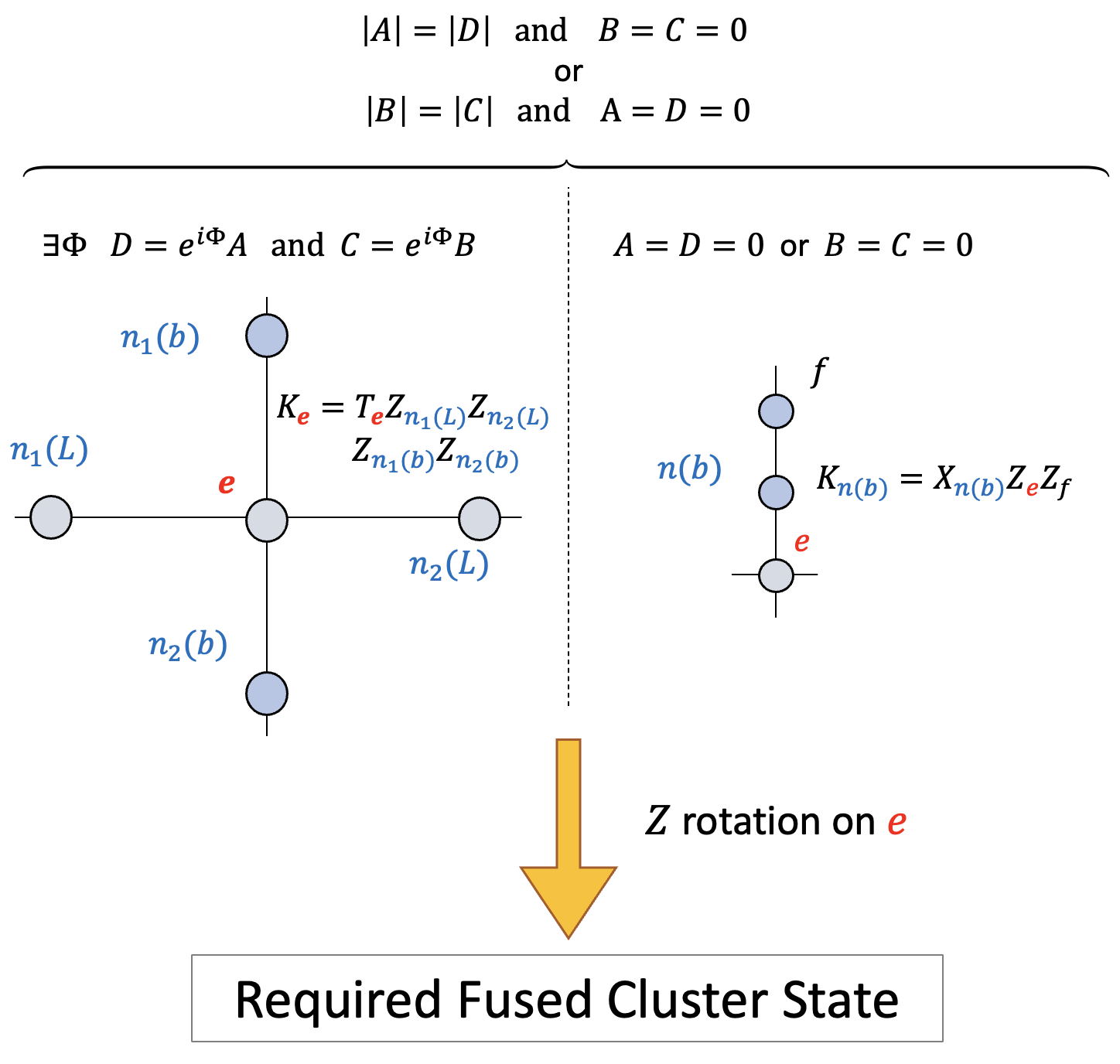
Appendix D Summary of Section III

Refer to caption
Figure 13: Summary of the results of section III. The black rectangle shows the general form of the final state. The red rectangle shows the results about Weighted graph states. The green rectangle illustrates the states that are cluster states up to 2-local rotation and the appropriate rotations. The yellow rectangle shows the stabilizer states.

We summarize in Figure 13 the resulting final states, that were discussed in section III. The general final state is written in the black rectangle (as in equation (26)), where its parameters $A,B,C,D$ depend on the elements of the matrix $U$, which represents the transformation of the creation operators of the qubits $a,b$ as in equation (22), and the result of the measurement of qubits $c,d$. The precise dependence is determined in equation (51). The wave function $\ket{\phi_{L}}_{V_{L}\setminus\{L\}}$ describes the total wave function of the one-dimensional cluster of the Logical qubit, without this qubit. The total wave function of this cluster is as in equation (6), and the wave function $\ket{\phi_{b}}_{V_{b}\setminus\{b\}}$ is defined similarly.

The yellow rectangle describes the final states, that are stabilizer states. In Theorem 1 we proved that the appropriate stabilizers (the generators of the group $S$ as in the definition of the stabilizer states) consist of the regular stabilizers $K_{a}^{\prime}$ as in equation (8) for aβ€²β‰ esuperscriptπ‘Žβ€²π‘’a^{\prime}\neq e, where for $e$ one has a new stabilizer as in (27). We identified these final states in theorem 1, as the states for which $A=D=0$ and $|B|=|C|$ or $B=C=0$ and $|A|=|D|$, and proved that these states become cluster states after operating with a single-qubit gate on $e$.

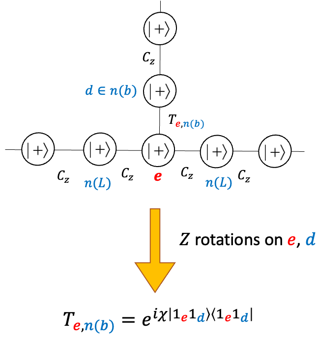
In Theorem 2 we obtained the conditions on $A,B,C,D$, such that if $|n(b)|=1$ the final state is Weighted graph state (if $|n(b)|=2$ then by the theorem this states are simply the stabilizer states). In the red rectangle there is the general form of the Weighted graph state. In this Weighted graph state, the qubits are put in the $\ket{+}$ state, and the edges are realized by $CZ$ gates between the proper qubits, as in the regular cluster state, except for the edge between $e$ and the qubit in $b$, for which the gate is (31), which also appears in the red rectangle.

The green rectangle shows the states, that are cluster states up to two-local rotations: two-qubit gate applied to the two qubits in $n(b)$, and a single-qubit gate on $e$. After the application of these gates, the resulting state is the required cluster state. In theorem 3 we proved that if $|n(b)|=1$, then these states (that are cluster states up to one-qubit rotations - one on $e$ and one on the single qubit of $n(b)$), are Weighted graph states. Furthermore, we proved in theorem 4, that these states are exactly the Weighted graph states with maximal entanglement entropy (still in the case $|n(b)|=1$).

Appendix E Summary of the results from sections IV and V that are not our main theorems

Table 2 summarizes results from sections IV and V, that were used to prove the main theorems in these sections, deduce the boundary values of $P(S)$ (46), and perform the numerical simulations in section VI.

$m_{i}=\left|U_{1i}\right|^{2}+\left|U_{2i}\right|^{2}\quad m_{1}+m_{2}+m_{3}+m_{4}=2$
$n_{i}=\frac{1}{2}-m_{i}\quad n_{1}+n_{2}+n_{3}+n_{4}=0$
$t_{i}=U_{1i}U_{2i}^{*}\quad t_{1}+t_{2}+t_{3}+t_{4}=0$
ki=|U1​i|2βˆ’|U2​i|2k1+k2+k3+k4=0formulae-sequencesubscriptπ‘˜π‘–superscriptsubscriptπ‘ˆ1𝑖2superscriptsubscriptπ‘ˆ2𝑖2subscriptπ‘˜1subscriptπ‘˜2subscriptπ‘˜3subscriptπ‘˜40k_{i}=\left|U_{1i}\right|^{2}-\left|U_{2i}\right|^{2}\quad k_{1}+k_{2}+k_{3}+k_{4}=0
The constants mi,ni,ti,kisubscriptπ‘šπ‘–subscript𝑛𝑖subscript𝑑𝑖subscriptπ‘˜π‘–m_{i},n_{i},t_{i},k_{i} that we defined (47) and their relations (48).
$|\phi\rangle_{ij}=\frac{1}{N_{ij}}\left(a_{ij}f_{1}f_{3}+b_{ij}f_{1}f_{4}+c_{ij}f_{2}f_{3}+d_{ij}f_{2}f_{4}\right)$ The wave function $\ket{\phi}_{ij}$ (50) of the relevant state $(i,j)$ (so iβ‰ j𝑖𝑗i\neq j).
$a_{ij}=U_{1i}U_{3j}+U_{1j}U_{3i}\quad b_{ij}=U_{1i}U_{4j}+U_{1j}U_{4i}$
$c_{ij}=U_{2i}U_{3j}+U_{2j}U_{3i}\quad d_{ij}=U_{2i}U_{4j}+U_{2j}U_{4i}$
Ni​j=|ai​j|2+|bi​j|2+|ci​j|2+|di​j|2=4​pi​jsubscript𝑁𝑖𝑗superscriptsubscriptπ‘Žπ‘–π‘—2superscriptsubscript𝑏𝑖𝑗2superscriptsubscript𝑐𝑖𝑗2superscriptsubscript𝑑𝑖𝑗24subscript𝑝𝑖𝑗N_{ij}=\sqrt{\left|a_{ij}\right|^{2}+\left|b_{ij}\right|^{2}+\left|c_{ij}\right|^{2}+\left|d_{ij}\right|^{2}}=\sqrt{4p_{ij}}
The coefficients ai​jsubscriptπ‘Žπ‘–π‘—a_{ij},bi​jsubscript𝑏𝑖𝑗b_{ij},ci​jsubscript𝑐𝑖𝑗c_{ij},di​jsubscript𝑑𝑖𝑗d_{ij} (51) and the normalization factor Ni​jsubscript𝑁𝑖𝑗N_{ij} (51) of the wave function (50) of the relevant state (i,j)𝑖𝑗(i,j).
$p_{ii}=\frac{1}{2}m_{i}\left(1-m_{i}\right)=\frac{1}{8}-\frac{1}{2}n_{i}^{2}$
pnon-relevantΒ =12​(1βˆ’n12βˆ’n22βˆ’n32βˆ’n42)≀12subscript𝑝non-relevantΒ 121superscriptsubscript𝑛12superscriptsubscript𝑛22superscriptsubscript𝑛32superscriptsubscript𝑛4212p_{\text{non-relevant }}=\frac{1}{2}\left(1-n_{1}^{2}-n_{2}^{2}-n_{3}^{2}-n_{4}^{2}\right)\leq\frac{1}{2}
The probability pi​isubscript𝑝𝑖𝑖p_{ii} to get to the non-relevant state (i,i)𝑖𝑖(i,i) (53) and the total probability for all the non-relevant states pn​o​nβˆ’r​e​l​e​v​a​n​tsubscriptπ‘π‘›π‘œπ‘›π‘Ÿπ‘’π‘™π‘’π‘£π‘Žπ‘›π‘‘p_{non-relevant} (54).
$p_{ij}=\frac{1}{8}-\frac{1}{2}n_{i}n_{j}-\frac{1}{2}\left|U_{1i}U_{1j}^{*}+U_{2i}U_{2j}^{*}\right|^{2}\leq\frac{1}{4}$ The probability $p_{ij}$ to get to the relevant state $(i,j)$ (52).
$\rho_{ij}=\frac{1}{N_{ij}^{2}}\begin{bmatrix}|a_{ij}|^{2}+|b_{ij}|^{2}&a_{ij}^{*}c_{ij}+b_{ij}^{*}d_{ij}\\ a_{ij}c_{ij}^{*}+b_{ij}d_{ij}^{*}&|c_{ij}|^{2}+|d_{ij}|^{2}\end{bmatrix}$ The reduced density matrix $\rho_{ij}$ (55).
$\operatorname{det}\left(\rho_{ij}\right)=\frac{\left|a_{ij}d_{ij}-b_{ij}c_{ij}\right|^{2}}{N_{ij}^{4}}=\left|\frac{\left(U_{1i}U_{2j}-U_{1j}U_{2i}\right)\left(U_{3j}U_{4i}-U_{3i}U_{4j}\right)}{4p_{ij}}\right|^{2}$ The determinant $\det(\rho_{ij})$ (57) of the reduced density matrix (55), which is monotonic in the entanglement entropy $S_{ij}$ (56).
$\lambda_{ij},1-\lambda_{ij}=\frac{1\pm\sqrt{1-4\operatorname{det}\left(\rho_{ij}\right)}}{2}$
Si​j=βˆ’Ξ»i​j​log2⁑λi​jβˆ’(1βˆ’Ξ»i​j)​log2⁑(1βˆ’Ξ»i​j)subscript𝑆𝑖𝑗subscriptπœ†π‘–π‘—subscript2subscriptπœ†π‘–π‘—1subscriptπœ†π‘–π‘—subscript21subscriptπœ†π‘–π‘—S_{ij}=-\lambda_{ij}\log_{2}\lambda_{ij}-\left(1-\lambda_{ij}\right)\log_{2}\left(1-\lambda_{ij}\right)
The computing of the eigenvalues Ξ»i​jsubscriptπœ†π‘–π‘—\lambda_{ij},1βˆ’Ξ»i​j1subscriptπœ†π‘–π‘—1-\lambda_{ij} (59) of the reduced density matrix (55) and the entanglement entropy Si​jsubscript𝑆𝑖𝑗S_{ij} (56) out of det⁑(ρi​j)subscriptπœŒπ‘–π‘—\det(\rho_{ij}) (57).
$S_{ij}=1\Leftrightarrow$ $0=a_{ij}c_{ij}^{*}+b_{ij}d_{ij}^{*}=2t_{i}n_{j}+2t_{j}n_{i}$ ,
0=|ai​j|2+|bi​j|2βˆ’|ci​j|2βˆ’|di​j|2=2​ni​kj+2​nj​ki0superscriptsubscriptπ‘Žπ‘–π‘—2superscriptsubscript𝑏𝑖𝑗2superscriptsubscript𝑐𝑖𝑗2superscriptsubscript𝑑𝑖𝑗22subscript𝑛𝑖subscriptπ‘˜π‘—2subscript𝑛𝑗subscriptπ‘˜π‘–0=\left|a_{ij}\right|^{2}+\left|b_{ij}\right|^{2}-\left|c_{ij}\right|^{2}-\left|d_{ij}\right|^{2}=2n_{i}k_{j}+2n_{j}k_{i}
The conditions for the relevant state (i,j)𝑖𝑗(i,j) to be maximally entangled (64),(65).
If $S_{ij}=1$ then $p_{ij}\leq\frac{1}{8}$ and $p_{ij}=\frac{1}{8}\Rightarrow n_{i}=n_{j}=0$ The upper bound on $p_{ij}$ for maximally entangled relevant state as proven in Lemma 7.
Table 2: Summary of the results from sections IV and V, that are needed to prove the main theorems.