Flat Posterior Does Matter
For Bayesian Transfer Learning

Abstract

The large-scale pre-trained neural network has achieved notable success in enhancing performance for downstream tasks. Another promising approach for generalization is Bayesian Neural Network (BNN), which integrates Bayesian methods into neural network architectures, offering advantages such as Bayesian Model averaging (BMA) and uncertainty quantification. Despite these benefits, transfer learning for BNNs has not been widely investigated and shows limited improvement. We hypothesize that this issue arises from the inability to find flat minima, which is crucial for generalization performance. To address this, we evaluate the sharpness of BNNs in various settings, revealing their insufficiency in seeking flat minima and the influence of flatness on BMA performance. Therefore, we propose Sharpness-aware Bayesian Model Averaging (SA-BMA), a Bayesian-fitting flat posterior seeking optimizer integrated with Bayesian transfer learning. SA-BMA calculates the divergence between posteriors in the parameter space, aligning with the nature of BNNs, and serves as a generalized version of existing sharpness-aware optimizers. We validate that SA-BMA improves generalization performance in few-shot classification and distribution shift scenarios by ensuring flatness.

1 Introduction

Generalization to unseen datasets is one of the primary goals of machine learning. One of the promising approaches is to utilize large-scale pre-trained models and transfer learning [1, 2]. Large-scale pre-trained models are adaptable to a new downstream task or dataset under the limited labeled dataset. There have been diverse works for transfer learning to enhance the ability of pre-trained models [3, 4, 5].

Another promising approach for better generalization is to utilize the Bayesian Neural Network (BNN) [6, 7, 8]. BNN integrates Bayesian statistical methods with neural network (NN) architectures by introducing uncertainty on the weights of the neural networks. BNN has two major advantages over the deterministic neural networks (DNN); Bayesian Model Averaging (BMA) [9, 10, 11, 12] and uncertainty quantification [13, 14]. These BNN properties are crucial for improved generalization performance under the limited training dataset [15]. Specifically, when the number of labeled datasets is limited, the error of the dataset (e.g., noisy label, noisy feature dataset) is more critical for overfitting, and uncertainty-aware is important.

Despite the promising potentials of BNN, transfer learning on BNN has been explored limitedly. Most transfer learning works have been studied only for DNN [4, 16]. These transfer learning methods enhance the generalization performance of DNN, but they are not directly compatible with BNN, stemming from the difference in nature between DNN and BNN. The previous transfer learning works in DNN focus on identifying the single parameter weights with high generalization performance, while BNN requires finding distribution of the weight parameters [17, 18]. Therefore, Bayesian transfer learning can be interpreted as a generalized version of transfer learning on DNN. Several works studied Bayesian transfer learning but showed limited improvement and inferior performance compared to fine-tuned DNN models. We hypothesize that this failure might be originated from the inability to capture the flat posterior.

Flatness is known to be one of the key factors that significantly impact generalization performance [19, 20, 21]. BNNs are also known as having flatness-aware property [22]. Some studies give attention to it to accelerate convergence through natural gradient [23] and generalize model better through flatness-aware optimization [24, 25] in Bayesian perspective. However, we cast doubt that BNNs cannot reflect the flatness without flat-seeking optimizer. To investigate this, we evaluate the sharpness of BNNs with various settings. We verify that the current BNN methods are insufficient to seek the flat posterior without a flatness-aware optimizer; therefore, they fail to achieve improved generalization performance compared to the DNN. Second, we show that flatness influences the performance of BMA, a distinctive inference method with posterior samples in approximated BNN. Through these steps, we conjecture that the flat posterior is one of the key factors of BNN.

Therefore, we propose a Bayesian-fitting flat posterior seeking optimizer, Sharpness-aware Bayesian Model Averaging (SA-BMA), in Bayesian transfer learning. We first compute the adversarial posterior that belongs to the vicinity of the current posterior through divergence, which maximizes the BNN loss function. After that, we update the posterior by employing the gradient of the adversarial posterior with respect to the BNN loss. SA-BMA captures the essence of BNNs by assessing the discrepancy between posteriors within the parameter space during the computation of the adversarial posterior, distinguishing itself from flat optimization methods based on DNNs. Along with the optimizer, we adopt Bayesian transfer learning scheme to approximate the flat posterior. We selectively optimize specific components of the model, such as the classifier and normalization layers, to ensure compatibility between SA-BMA and large-scale pre-trained models. This approach enables SA-BMA to improve the generalization capabilities of BNN with minimal additional computational overhead. Furthermore, we show that the proposed SA-BMA is an extended version of previous flatness-aware optimizers, Sharpness-aware Minimization (SAM), Fisher SAM (FSAM), and natural gradient (NG) with specific conditions. We validate the superiority of SA-BMA in few-shot classification tasks and distributional shift settings. Also, we verify the flat posterior of SA-BMA with loss landscape visualization and Hessian eigenvalue comparison.

Our major contributions are summarized as follows:

• We point out that the limited improvement of Bayesian transfer learning stems from the sharpness of the posterior and show that pre-existed BNN frameworks cannot guarantee the flatness. Also, we observe the influence of flatness on the performance of BMA and prove that the sharpness of sampled models affects the sharpness of the averaged model.

• Based on the importance of flat posterior, we suggest a Bayesian-fitting flat posterior seeking optimizer, SA-BMA. SA-BMA is a parameter space loss geometric optimizer that fine-tunes pre-trained models and able to approximate other loss geometric optimizers, such as SAM, FSAM, and NG.

• We validate that SA-BAM seeks flat-posterior; therefore, SA-BMA achieves improved performance on few-shot learning and distribution shift settings.

2 Preliminary

2.1 Bayesian Neural Networks

BNNs aim to estimate the posterior distribution $p(w|\mathcal{D})$ of model parameters $w\subseteq\mathbb{R}^{p}$ with observed data points $\mathcal{D}=\{(x,y)\}$ with inputs $x$ and outputs $y$. The posterior distribution $p(w|\mathcal{D})$ is calculated by Bayes’ Rule:

$$p(w|\mathcal{D})=\frac{p(\mathcal{D}|w)p(w|x)}{\int_{w}p(\mathcal{D}|w)p(w|x)dw}$$ (1)

where $p(\mathcal{D}|w)$ and $p(w|x)$ denote the likelihood of data $\mathcal{D}$ and the prior distribution over $w$, respectively. Due to the high dimensionality of neural networks, it is intractable to compute the marginal likelihood (evidence) of Equation (1).

Numerous studies have focused on approximating the posterior $p(w|\mathcal{D})$ with variational parameter $\theta\subseteq\mathbb{R}^{q}$ as $p_{\theta}(w|\mathcal{D})$, including Markov Chain Monte Carlo (MCMC) [26, 27], Variational Inference (VI) [28, 29, 30], and other variants employing DNN [31, 32, 33, 34, 35].

Based on the approximated posterior, BNNs make predictions of the model on unobserved data $(x^{*},y^{*})$ through Bayesian Model Averaging (BMA):

$$p(y^{*}|x^{*},\mathcal{D}) =\int_{w}p(y^{*}|x^{*},w)p_{\theta}(w|\mathcal{D})dw$$ (2)

$$\approx\frac{1}{M}\sum_{i=1}^{M}p(y^{*}|x^{*},w_{i}),\ \ w_{i}\sim p_{\theta}(w|\mathcal{D})$$ (3)

where $M$ denotes the number of sampled models. Unfortunately, the integral in Equation (2) is intractable. Monte Carlo (MC) integration (Equation (3)) is a representative method to approximate posterior predictive. BNNs marginalize diverse solutions over the posterior of model parameters through BMA.

2.2 Flatness and Optimizers

Many studies have connected the correlation between the flatness of loss surface and generalization [36, 19, 20, 21]. The eigenvalues of the model Hessian is a widely adopted method for measuring the flatness, as smaller eigenvalues indicate flatter regions in the loss landscape. However, due to the large size of neural network, it is impractical to examine all eigenvalues. Therefore, maximal eigenvalue $\lambda_{1}$ or ratio of eigenvalue $\lambda_{1}/\lambda_{5}$ is often used to compare model flatness, where $\lambda_{i}$ denotes $i$-th maximal eigenvalue [20, 37, 38].

On the top of the connection between flatness and generalization, the local entropy [39, 40] is one way to find flat minima. Typically, Entropy-SGD [41] and Entropy-SGLD [42] suggested finding flat modes by approximating the local entropy with a nested chain. On the other hand, recently, SAM [37] proposed to capture the sharpness as the difference between the empirical loss and the worst-case loss within the neighborhood $\gamma$ in the first step. Formally, within $\gamma$-ball neighborhood, the loss function of SAM $l_{SAM}^{\gamma}$ is defined as:

$$l^{\gamma}_{\text{SAM}}(w)=\min_{w}\max_{\|\Delta w_{\text{SAM}}\|_{p}\leq\gamma}l(w+\Delta w)$$ (4)

where $l(\cdot)$ is the original loss function and practically set $p=2$. A closed-form solution of Equation (4) can be calculated by approximating $l(w+\Delta w)$ through first-order Taylor approximation. In L2 norm, the solution becomes:

$$\Delta w_{\text{SAM}}=\gamma\frac{\nabla_{w}l(w)}{\|\nabla_{w}l(w)\|_{2}}$$

In the second step, SAM updates the model parameter $w$ by using the gradient of perturbated set $w+\Delta w_{\text{SAM}}$:

$$\nabla_{w}l_{\text{SAM}}^{\gamma}(w)\approx\nabla_{w}l(w+\Delta w_{\text{SAM}})$$

On the one hand, FSAM [43] suggested natural non-Euclidean parameter space with Fisher information induced distance metric $F_{y}(w):\mathbb{R}^{p}\rightarrow\mathbb{R}^{p}$ to calculate perturbation ball:

$$l^{\gamma}_{\text{FSAM}}(w)=\min_{w}\max_{\|F_{y}(w)^{-1}\Delta w\|_{p}\leq\gamma^{2}}l(w+\Delta w)$$

where Fisher Information Matrix (FIM) $F_{y}(w)=Diag\big{(}\mathbb{E}_{x,y}[\nabla_{w}\log p(y|x,w)\nabla_{w}\log p(y|x,w)^{T}]\big{)}$ and $Diag$ denotes extracting diagonal term in matrix. In other words, by preconditioning FIM $F_{y}(w)$ over predictive distribution, FSAM attempts to find curvature-aware perturbation. The perturbation from inner maximization step is solved with gradient:

$$\Delta w_{\text{FSAM}}=\gamma\frac{F_{y}(w)^{-1}\nabla_{w}l(w)}{\|F_{y}(w)^{-1/2}\nabla_{w}l(w)\|_{2}}$$

Note that the $F_{y}(w)$ is defined in predictive distribution $p(y|x,w)$ under deterministic model parameter $w$. In addition to the studies for distance metric in the neighborhood of SAM, there are trials to make SAM more efficient [44, 45, 46, 47]. Particularly, SAM-ON [48] only takes an adversarial step in normalization layers.

3 Flatness Does Matter For Bayesian Model Averaging?

It is well-known that a model in flat minima shows better generalization performance [19, 20, 21]. Based on the correlation between the flatness and generalization, we question whether the BNNs can reflect the flatness. To answer this question, we evaluate the sharpness of BNN with diverse settings and show that it can fail to capture the loss geometry well. We also show the performance of BMA can become stagnant or degraded without considering the flatness. Additionally, we theoretically prove the sharpness bound of BMA and justify that it is necessary to take flatness into account.

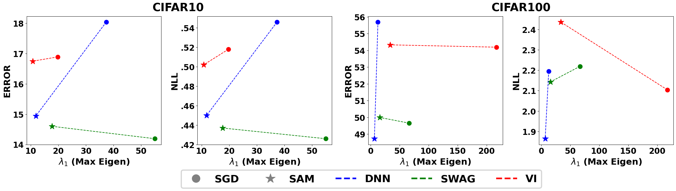
Figure 1: Variations in performance and flatness based on different optimizers. We measured the Error and NLL, lower is better, for the CIFAR10 and CIFAR100. For flatness, we utilize the maximal eigenvalue $\lambda_{1}$, where lower values indicate flatter model. We adopt SWAG and VI as BNN frameworks. Firstly, it suggests that BNNs may not consistently capture the loss geometry effectively. Secondly, the disparity in generalization performance between SGD and the flat-seeking optimizer SAM in BNNs is not significant. In other words, switching from SGD to SAM in BNNs results in only a slight improvement in generalization.

3.1 BNN and Flatness

To begin with, we measure the flatness and generalization performance of BNN with diverse learning rate schedulers. Furthermore, we compare the performance and flatness according to whether SAM is applied or not. For flatness, we set $\lambda_{1}$ and $\lambda_{1}/\lambda_{5}$ as criterion [37, 24]. In case of BMA, we average the maximal eigenvalue $\lambda_{1}$ and the ratio $\lambda_{1}/\lambda_{5}$ of each model’s Hessian, respectively. We also measure the Accuracy ($100-\text{Error}$), Expected Calibration Error (ECE) [49], and Negative Log Likelihood (NLL) to compare the generalization ability. We mainly set ResNet18 (RN18) [50] without Batch Normalization (BN) [51] as a backbone model. For BNN framework, we adopt VI and SWAG. To reduce the effect on measuring the flatness, we remove the BN and also do not adjust data augmentation. We present more detailed results of the analysis between flatness and performance across various settings in Appendix A.1, demonstrating consistent outcomes.

Figure 1 illustrates the performance and flatness variations in both DNN and BNNs based on different optimizers. Firstly, it is evident from Figure 1 that BNNs do not consistently capture the loss geometry well. BNNs trained with SGD often exhibit higher $lambda_{1}$ compared to DNN trained with SGD, and they show significantly higher $lambda_{1}$ when compared to DNN trained with SAM. Secondly, the transition from SGD to SAM in BNN results in only marginal enhancement in generalization. This contrasts with the significant improvement observed in both flatness and generalization performance in DNN. Our findings suggest that the inherent disparities between BNN and DNN mean that simply employing SAM, which is tailored for DNN, often fails to leverage generalization improvements effectively in BNN. Our experiments indicate that BNNs do not inherently guarantee flatness, and the naive adaptation of SAM for DNN may not be sufficient to enhance their generalizability.

3.2 BMA and Flatness

BNNs possess the benefit of BMA, which anticipates performance enhancement through model ensemble based on the approximated posterior distribution. However, following the fact that BNNs do not guarantee flatness, we cast another question: "Does the flatness also affect BMA?"

First, we consolidate that the correlation between flatness and generalization performance also exists in BMA. Figure 2(a) shows the affirmative correlation between performance and flatness throughout $30$ sampled model parameters from posterior trained on CIFAR10 with RN18 w/o BN. Models trained with constant learning rate consist of Figure 2(a), and we provide additional plots in Figure 7 (Appendix A.2), demonstrating consistent results.

(a) Correlation between flatness and generalization

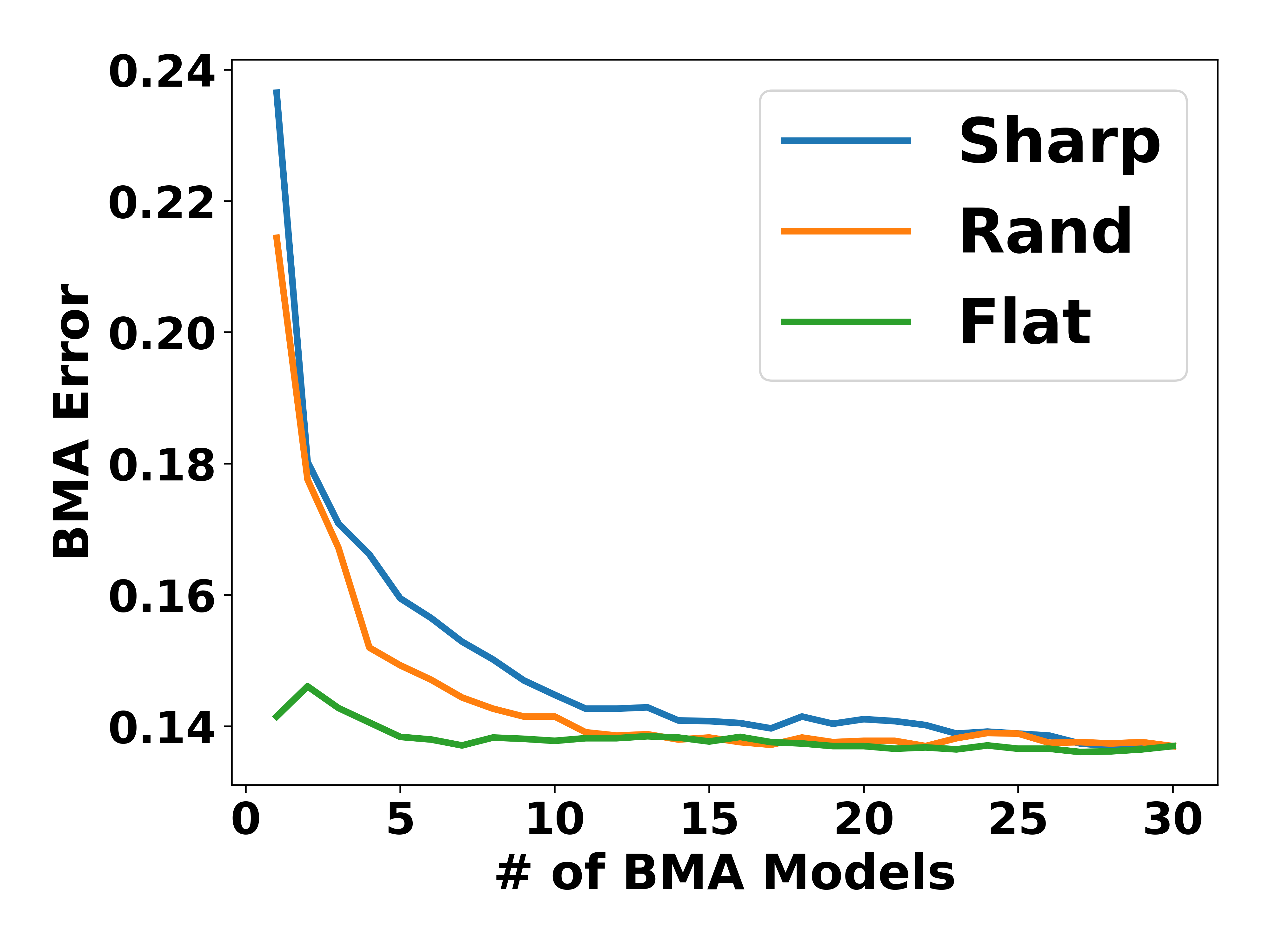
(b) Error variation under flatness-ordered BMA

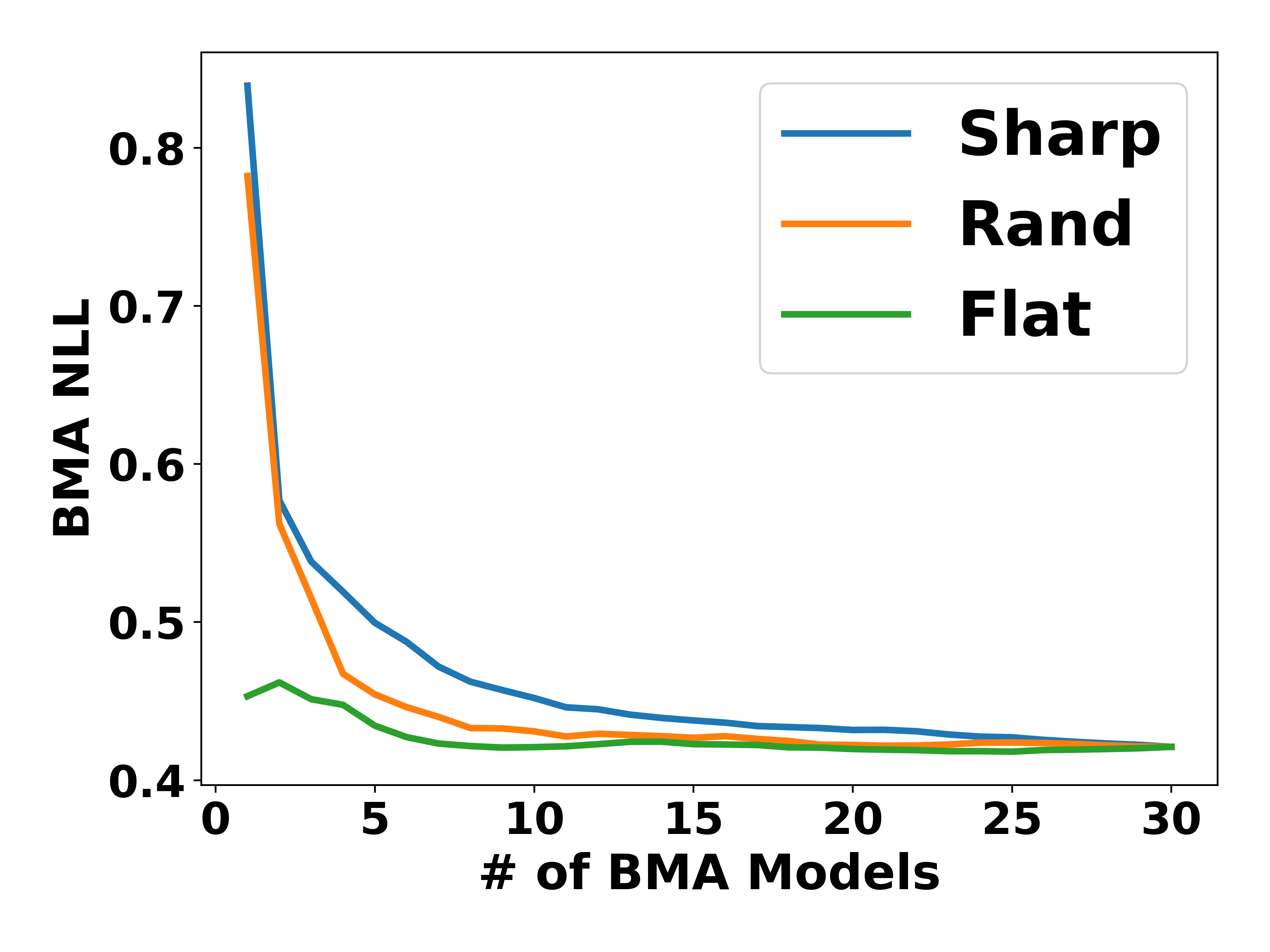
(c) NLL variation under flatness-ordered BMA

Figure 2: (a) shows the distinct correlation between flatness, maximal eigenvalue of model Hessian ($\lambda_{1}$), and normalized generalization metrics, classification error, ECE, and NLL. $\rho$ depicts the Pearson correlation coefficient. We conjecture that the flatness is crucial for the generalization performance of BNN. (b)-(c) represent the variation of generalization performance under flatness-ordered BMA. "Flat" denotes starting model averaging from the flattest model, and "Sharp" means the opposite of "Flat". "Rand" denotes starting BMA from a random sample of prepared 30 models. This result shows degradation or stagnant can appear without considering the flatness in BMA.

Second, we observe how performance changes when the sampling model parameter in BMA is performed based on flatness. Figure 2(b)-2(c) shows the influence of flatness on BMA performance. We first sample $30$ models trained on CIFAR10 with RN18 w/o BN. Then, we start to do BMA through three criteria. "Flat" denotes starting model averaging from the flattest model, and "Sharp" means the opposite of "Flat". "Rand" denotes starting BMA from a random sample of prepared $30$ models. From Figure 2(b)-2(c), we conclude that degradation or stagnation can appear without considering the flatness during BMA. Figure 8 and 9 (Appendix A.3) support the conclusion, as well. With a closer look at the "Flat" label, where progressively sharper models are contained, we observe that performances do not improve as the number of averaged models increases. These points prove the necessity of flatness in BMA.

Through various experiments in Section 3.1 and 3.2, we show that existing BNN often fails to capture the loss geometry and the flatness influences on BMA performance. In this part, we also suggest a theoretical bound of flatness on BMA through the eigenvalue of model Hessian. Note that the eigenvalue of model Hessian is a typical measurement to compare the flatness of neural networks. In case sampling $M$ models to BMA, let Hessian of each model sample as $A_{i},i=1,...,M$. We assume the $A_{i}$ as the $p\times p$ Hermitian matrices and the Hessian of a sampled model. $\lambda_{\max}(A_{i})$ and $\lambda_{\min}(A_{i})$ denote the maximal and minimal eigenvalue of $A_{i}$, respectively. $A$ is a simple arithmetic average of $M$ matrices $A_{i},i=1,...,M$, and is also a Hermitian following the property of Hermitian. $A$ is the Hessian of the averaged model. Through Weyl’s inequality [52], the bound of the eigenvalue of $A$ is defined as:

Theorem 1.

With $M$ Hermitian matrices $A_{i},i=1,...,M$, the maximal eigenvalue of averaged matrix $A=1/M\sum_{i=1}^{M}A_{i}$ is bounded as follow:

$$\max\left(\Bigg{\{}\frac{1}{M}\bigg{(}\lambda_{\max}(A_{i})+\sum_{\begin{subarray}{c}j=1\\ j\neq i\end{subarray}}^{M}\lambda_{\min}(A_{j})\bigg{)}\Bigg{\}}_{i=1}^{M}\right)\leq\lambda_{\max}(A)\leq\frac{\sum_{i=1}^{M}\lambda_{\max}(A_{i})}{M}$$ (5)

Theorem 1 implies that the flatness of averaged model reflects the flatness of model samples. If a sampled model had a large eigenvalue of Hessian, the lower bound of Hessian eigenvalue can be larger. Namely, the ensembled model can be located in a sharp region if it settles in sharp minima, leading the model to degraded generalization performance. On the contrary, the model averaged with flat minima models can get a tighter upper bound of Hessian eigenvalue, leading to better generalization. This theoretical sharpness bound of BMA can support the necessity of considering flatness on BMA, along with experimental backup.

4 Bayesian Model Averaging With Flat Posterior

For more effective BMA, we propose a Bayesian flat-seeking optimizer (Section 4.1) and Bayesian transfer learning that can be combined with diverse BNN frameworks (Section 4.2).

4.1 Bayesian Flat-seeking Optimizer

Simply applying SAM into BNN cannot be adequate considering the nature of BNN, which estimates a distribution rather than a point of the model parameters (Section 3.1). To deal with the nature of BNN, we suggest a new objective function:

$$l_{\text{SA-BMA}}^{\gamma}(\theta)=\min_{\theta}\max_{d|\theta+\Delta\theta,\theta|\leq\gamma^{2}}l(\theta+\Delta\theta)$$ (6)

$$\textrm{s.t.}\ \ d|\theta+\Delta\theta,\theta|=D_{KL}\big{[}p_{\theta+\Delta\theta}(w|\mathcal{D})\ ||\ p_{\theta}(w|\mathcal{D})\big{]}$$ (7)

where $\theta$ and $\Delta\theta$ denote the variational parameters and perturbation on them, respectively. For better understanding, we can assume the model parameters to follow the Gaussian distribution $\mathcal{N}(\mu,\Sigma)$; therefore, $\theta$ becomes the mean $\mu$ and covariance $\Sigma$.

Through the relationship between KL divergence and FIM, the objective function (Equation (6)) is rewritten as:

$$l^{\gamma}_{\text{SA-BMA}}(\theta)=\min_{\theta}\max_{\Delta\theta^{T}F_{\theta}(\theta)\Delta\theta\leq\gamma^{2}}l(\theta+\Delta\theta)$$ (8)

where $F_{\theta}({\theta})=\mathbb{E}_{w,\mathcal{D}}[\nabla_{\theta}\log p_{\theta}(w|\mathcal{D})\nabla_{\theta}\log p_{\theta}(w|\mathcal{D})^{T}]$. Note the FIM is defined over parameters, directly.

After the first Taylor Expansion on $l(\theta+\Delta\theta)$ in Equation (8), we express the maximize problem as a Lagrangian dual problem:

$$L(\Delta\theta,\lambda)=l(\theta)+\nabla l_{\theta}(\theta)^{T}\Delta\theta-\lambda(\Delta\theta^{T}F_{\theta}(\theta)\Delta\theta-\gamma^{2})$$ (9)

From Equation (9), we get the optimal value $\Delta\theta_{\text{SA-BMA}}$ as:

$$\Delta\theta_{\text{SA-BMA}}=\gamma\frac{F_{\theta}(\theta)^{-1}\nabla_{\theta}l(\theta)}{\sqrt{\nabla_{\theta}l(\theta)^{T}F_{\theta}(\theta)^{-1}\nabla_{\theta}l(\theta)}}$$ (10)

We update $\theta$ by gradients from points perturbated with $\Delta\theta_{\text{SA-BMA}}$:

$$\nabla_{\theta}l^{\gamma}_{\text{SA-BMA}}(\theta)\approx\nabla_{\theta}l(\theta+\Delta\theta_{\text{SA-BMA}})$$ (11)

Detailed formula derivation of the opitmal perburation for SA-BMA is provided in Appendix C.2.

Notably, SA-BMA is a generalized version of SAM, FSAM, and NG under deterministic parameters, as shown in Theorem 2. In detail, using the diagonal FIM makes it equivalent to FSAM, and using the identity FIM makes it equivalent to SAM. Additionally, using a specific learning rate makes it equivalent to NG. Proof of Theorem 2 are provided in Appendix C.3.

Theorem 2.

Suppose the model parameter $w$ is deterministic and the loss function $l(\cdot)$ is twice continuously differentiable. Let $p\times p$ invertible $\gamma^{\prime}=\gamma/\sqrt{\nabla_{\theta}l(\theta)^{T}F_{\theta}(\theta)^{-1}\nabla_{\theta}l(\theta)}$, then

1. $\Delta\theta_{\text{SA-BMA}}$ degenerates to $\Delta\theta_{\text{FSAM}}$ by using the diagonal terms of FIM.

2. $\Delta\theta_{\text{SA-BMA}}$ degenerates to $\Delta\theta_{\text{SAM}}$ by using identity matrix as FIM.

3. Update rule of SA-BMA $\theta-\eta_{\text{SA-BMA}}\nabla_{\theta}l(\theta+\Delta\theta)$ degenerates to update rule of NG
   $\theta-\eta_{\text{NG}}F_{y}(\theta)^{-1}\nabla_{\theta}l(\theta)$ with learning rate $\eta_{\text{SA-BMA}}=\eta_{\text{NG}}{(I+\gamma^{\prime})}^{-1}F_{\theta}(\theta)^{-1}$

4.2 Bayesian Transfer Learning

Along with the proposed Bayesian sharpness-aware optimizer, we suggest Bayesian framework-agnostic transfer learning as well. The proposed Bayesian transfer learning scheme consists of three steps and Algorithm 1 (Appendix B.2) depicts how it operates.

First, we load a pre-trained model on the source task and change the loaded DNN into BNN on the source or downstream task. Various BNN frameworks such as VI, SWAG, and others can be employed to transform a DNN into a BNN. This study mainly employs SWAG and MOPED for VI.

After that, we train the subnetwork of the converted BNN model with the proposed optimizer. Unfortunately, calculating the gradient of the log posterior for the entire model parameters is intractable. Thus, we adopt a subnetwork BNN strategy, which has been actively studied to alleviate the computational load for BNN [53, 54, 55, 56, 57, 58], and they often accomplish better performance than full-training. Formally, we select partial trainable parameters $w_{s}\subseteq\mathbb{R}^{p_{1}}$ and freeze remain parameters $w_{f}\subseteq\mathbb{R}^{p_{2}}$, where $w_{s}\cup w_{f}=w$ and $p_{1}+p_{2}=p$. This study chiefly composes the trainable parameters with the normalization and last layers. We set the simple Gaussian distribution $\mathcal{N}(0,\alpha I)$ for the last layer, where $\alpha$ is a hyperparameter to scale the variance of last layer. Through this scheme, we can expect scalable and stable training using pre-trained models.

5 Experiments

5.1 Few-shot image classification

We mainly measure the performance of the proposed SA-BMA in few-shot image classification task. First, we train our model in CIFAR10 and CIFAR100 [59] with ten images per class, each. We compare our model SA-BMA to the sharpness-aware baseline SAM, FSAM, SWAG, F-SWAG [60], E-MCMC [24], and bSAM [25] and the Bayesian transfer learning baseline MOPED [61] and Pre-Train Your Loss (PTL) [15]. We consider accuracy (ACC), expected calibration error (ECE), and negative log likelihood (NLL) as metrics for generalization. We report the performance of predictive distributions, which we approximate using Bayesian Model Averaging (BMA) over 30 models sampled from a posterior distribution. In this experiment, we adopt RN18 [50] and ViT-B/16 [62] pre-trained on ImageNet (IN) 1K [63] as backbone. Detailed configuration for each baseline is provided in Appendix B and code is provided in https://anonymous.4open.science/r/SA-BMA-A890.

Table 1: Downstream task performance with RN18 and ViT-B/16 pre-trained on IN 1K. SA-BMA (SWAG) and SA-BMA (VI) denote using SWAG and VI to convert pre-trained model into BNN, respectively. Bold and underline denote best and second best performance each. SA-BMA shows superior performance both on the CIFAR10 and CIFAR100 10-shot, with the sole exception being the ECE on the CIFAR100 10-shot in RN18.

Backbone RN18 ViT-B/16 Dataset CIFAR10 10-shot CIFAR100 10-shot CIFAR10 10-shot CIFAR100 10-shot Method Optim ACC $\uparrow$ ECE $\downarrow$ NLL $\downarrow$ ACC $\uparrow$ ECE $\downarrow$ NLL $\downarrow$ ACC $\uparrow$ ECE $\downarrow$ NLL $\downarrow$ ACC $\uparrow$ ECE $\downarrow$ NLL $\downarrow$ DNN SGD $55.52_{\pm 0.32}$ $0.062_{\pm 0.006}$ $1.302_{\pm 0.020}$ $44.29_{\pm 0.83}$ $\textbf{0.025}_{\pm 0.005}$ $2.133_{\pm 0.043}$ $84.37_{\pm 1.47}$ $0.056_{\pm 0.061}$ $0.503_{\pm 0.038}$ $68.78_{\pm 0.21}$ $0.143_{\pm 0.007}$ $1.193_{\pm 0.019}$ SAM $56.54_{\pm 2.57}$ $0.129_{\pm 0.013}$ $1.354_{\pm 0.089}$ $44.51_{\pm 0.07}$ $0.065_{\pm 0.007}$ $2.089_{\pm 0.013}$ $84.35_{\pm 0.81}$ $0.035_{\pm 0.012}$ $0.486_{\pm 0.023}$ $68.93_{\pm 0.37}$ $0.153_{\pm 0.005}$ $1.200_{\pm 0.021}$ FSAM $54.04_{\pm 4.11}$ $0.139_{\pm 0.010}$ $1.432_{\pm 0.068}$ $44.07_{\pm 1.21}$ $0.056_{\pm 0.005}$ $2.159_{\pm 0.064}$ $84.51_{\pm 0.50}$ $0.073_{\pm 0.085}$ $0.517_{\pm 0.061}$ $68.74_{\pm 0.39}$ $0.110_{\pm 0.007}$ $1.166_{\pm 0.024}$ SWAG SGD $56.31_{\pm 0.60}$ $0.094_{\pm 0.013}$ $1.315_{\pm 0.056}$ $44.14_{\pm 1.28}$ $0.034_{\pm 0.010}$ $2.161_{\pm 0.058}$ $83.51_{\pm 2.22}$ $0.022_{\pm 0.015}$ $0.510_{\pm 0.072}$ $68.72_{\pm 0.45}$ $0.065_{\pm 0.005}$ $1.136_{\pm 0.014}$ F-SWAG SAM $57.65_{\pm 1.20}$ $0.075_{\pm 0.003}$ $1.249_{\pm 0.038}$ $46.09_{\pm 0.44}$ $0.062_{\pm 0.006}$ $2.089_{\pm 0.002}$ $83.87_{\pm 1.28}$ $\underline{0.013}_{\pm 0.005}$ $0.492_{\pm 0.040}$ $68.84_{\pm 0.77}$ $0.076_{\pm 0.012}$ $1.137_{\pm 0.020}$ VI bSAM $56.56_{\pm 1.18}$ $0.083_{\pm 0.006}$ $1.280_{\pm 0.027}$ $43.93_{\pm 0.48}$ $0.060_{\pm 0.003}$ $2.167_{\pm 0.026}$ $82.85_{\pm 2.10}$ $0.113_{\pm 0.008}$ $0.583_{\pm 0.062}$ $68.42_{\pm 0.40}$ $0.148_{\pm 0.019}$ $1.219_{\pm 0.031}$ MOPED SGD $57.29_{\pm 1.20}$ $0.093_{\pm 0.006}$ $1.297_{\pm 0.045}$ $44.30_{\pm 0.42}$ $0.047_{\pm 0.006}$ $2.127_{\pm 0.005}$ - - - - - - E-MCMC SGLD $56.69_{\pm 2.14}$ $0.142_{\pm 0.004}$ $1.266_{\pm 0.054}$ $41.57_{\pm 0.04}$ $\underline{0.046}_{\pm 0.012}$ $2.370_{\pm 0.175}$ $83.91_{\pm 1.16}$ $0.333_{\pm 0.010}$ $0.877_{\pm 0.044}$ $63.40_{\pm 0.01}$ $0.280_{\pm 0.008}$ $1.655_{\pm 0.024}$ PTL SGLD $57.26_{\pm 1.44}$ $0.116_{\pm 0.003}$ $1.345_{\pm 0.004}$ $43.00_{\pm 1.05}$ $0.120_{\pm 0.006}$ $2.383_{\pm 0.062}$ $85.76_{\pm 1.37}$ $0.080_{\pm 0.014}$ $0.482_{\pm 0.027}$ $65.52_{\pm 2.45}$ $\underline{0.056}_{\pm 0.006}$ $1.260_{\pm 0.095}$ SA-BMA (SWAG) $\underline{61.79}_{\pm 4.34}$ $\underline{0.026}_{\pm 0.004}$ $\underline{1.214}_{\pm 0.119}$ $\underline{47.45}_{\pm 0.60}$ $0.055_{\pm 0.018}$ $\underline{2.044}_{\pm 0.022}$ $\underline{86.81}_{\pm 0.78}$ $\textbf{0.010}_{\pm 0.003}$ $\underline{0.399}_{\pm 0.034}$ $\underline{70.10}_{\pm 0.18}$ $\textbf{0.045}_{\pm 0.015}$ $\underline{1.063}_{\pm 0.023}$ SA-BMA (VI) $\textbf{64.98}_{\pm 1.37}$ $\textbf{0.016}_{\pm 0.007}$ $\textbf{0.997}_{\pm 0.046}$ $\textbf{49.09}_{\pm 1.38}$ $0.071_{\pm 0.004}$ $\textbf{1.893}_{\pm 0.036}$ $\textbf{87.56}_{\pm 1.10}$ $0.044_{\pm 0.012}$ $\textbf{0.397}_{\pm 0.026}$ $\textbf{71.37}_{\pm 0.36}$ $0.060_{\pm 0.007}$ $\textbf{1.023}_{\pm 0.012}$

Table 2: Downstream task accuracy with RN50 and ViT-B/16 pre-trained on IN 1K. SA-BMA (SWAG) denotes using SWAG to convert pre-trained model into BNN. Bold and underline denote best and second best performance each. SA-BMA demonstrates superior performance across all 16-shot datasets, including EuroSAT [64], Flowers102 [65], Pets [66], and UCF101 [67].

Backbone RN50 ViT-B/16 Method Optim EuroSAT Flowers102 Pets UCF101 Avg EuroSAT Flowers102 Pets UCF101 Avg DNN SGD $86.75_{\pm 1.47}$ $93.16_{\pm 0.27}$ $89.95_{\pm 0.51}$ $66.34_{\pm 0.59}$ $84.05_{\pm 0.33}$ $81.25_{\pm 1.03}$ $91.24_{\pm 0.83}$ $88.68_{\pm 0.92}$ $68.64_{\pm 0.51}$ $82.45_{\pm 0.56}$ DNN SAM $87.85_{\pm 0.49}$ $94.80_{\pm 0.17}$ $90.23_{\pm 0.78}$ $70.40_{\pm 0.76}$ $85.82_{\pm 0.25}$ $82.53_{\pm 0.65}$ $\underline{93.08}_{\pm 0.87}$ $\underline{90.66}_{\pm 0.74}$ $\underline{70.66}_{\pm 1.03}$ $\underline{84.23}_{\pm 0.60}$ SWAG SGD $88.97_{\pm 1.56}$ $93.27_{\pm 0.15}$ $89.95_{\pm 0.46}$ $66.41_{\pm 0.30}$ $84.65_{\pm 0.37}$ $81.62_{\pm 0.66}$ $91.21_{\pm 0.91}$ $88.67_{\pm 0.42}$ $67.65_{\pm 0.45}$ $82.29_{\pm 0.31}$ F-SWAG SAM $90.03_{\pm 1.08}$ $\underline{94.84}_{\pm 0.26}$ $\underline{90.12}_{\pm 0.57}$ $\underline{70.00}_{\pm 0.87}$ $\underline{86.25}_{\pm 0.19}$ $\underline{82.72}_{\pm 0.49}$ $92.93_{\pm 0.93}$ $90.60_{\pm 0.55}$ $68.67_{\pm 0.39}$ $83.73_{\pm 0.35}$ MOPED SGD $85.21_{\pm 3.14}$ $92.15_{\pm 0.73}$ $89.25_{\pm 0.61}$ $65.85_{\pm 0.99}$ $83.11_{\pm 0.86}$ - - - - - PTL SGLD $\underline{90.01}_{\pm 0.39}$ $92.55_{\pm 0.53}$ $89.43_{\pm 0.41}$ $65.00_{\pm 1.24}$ $84.25_{\pm 0.30}$ $83.76_{\pm 0.61}$ $88.43_{\pm 1.27}$ $88.54_{\pm 0.53}$ $60.38_{\pm 1.84}$ $80.28_{\pm 0.03}$ SABMA (SWAG) SABMA $\bm{90.16}_{\pm 1.04}$ $\bm{95.85}_{\pm 1.26}$ $\bm{90.23}_{\pm 0.58}$ $\bm{71.57}_{\pm 0.27}$ $\bm{86.95}_{\pm 0.65}$ $\bm{84.60}_{\pm 0.25}$ $\bm{94.15}_{\pm 0.80}$ $\bm{91.30}_{\pm 0.25}$ $\bm{72.63}_{\pm 1.12}$ $\bm{85.67}_{\pm 0.14}$

Table 3: Downstream task accuracy of CLIP with visual encoder, RN50 and ViT-B/16. SA-BMA (SWAG) denote employing SWAG to convert the last layer of visual encoder. IN-V2, IN-R, IN-A, and IN-S mean ImageNet-V2 [68], ImageNet-R [69], ImageNet-A [70], and ImageNet-Sketch [71], respectively. Bold and underline denote best and second best performance each. SA-BMA shows superior performance in average over five datasets.

Backbone Method Optim IN IN-V2 IN-R IN-A IN-S Avg RN50 ZS - $59.83_{\pm 0.00}$ $52.89_{\pm 0.00}$ $60.73_{\pm 0.00}$ $\underline{23.25}_{\pm 0.00}$ $35.45_{\pm 0.00}$ $46.43_{\pm 0.00}$ DNN SGD $61.70_{\pm 0.01}$ $54.31_{\pm 0.01}$ $60.87_{\pm 0.01}$ $22.74_{\pm 0.01}$ $\underline{35.68}_{\pm 0.00}$ $47.06_{\pm 0.01}$ DNN SAM $61.73_{\pm 0.01}$ $\underline{54.35}_{\pm 0.01}$ $60.86_{\pm 0.01}$ $22.76_{\pm 0.01}$ $35.67_{\pm 0.00}$ $47.07_{\pm 0.01}$ SWAG SGD $\underline{61.77}_{\pm 0.22}$ $54.10_{\pm 0.19}$ $\textbf{61.25}_{\pm 0.21}$ $\textbf{23.25}_{\pm 0.08}$ $35.55_{\pm 0.27}$ $\underline{47.18}_{\pm 0.19}$ SA-BMA (SWAG) $\textbf{63.33}_{\pm 0.92}$ $\textbf{55.06}_{\pm 0.79}$ $\underline{61.14}_{\pm 0.37}$ $22.78_{\pm 0.68}$ $\textbf{35.82}_{\pm 0.11}$ $\textbf{47.63}_{\pm 0.17}$ ViT-B/16 ZS - $68.33_{\pm 0.00}$ $61.91_{\pm 0.00}$ $77.71_{\pm 0.00}$ $49.93_{\pm 0.00}$ $48.22_{\pm 0.00}$ $61.22_{\pm 0.00}$ DNN SGD $69.97_{\pm 0.00}$ $62.97_{\pm 0.01}$ $78.05_{\pm 0.00}$ $50.31_{\pm 0.02}$ $48.76_{\pm 0.00}$ $62.01_{\pm 0.00}$ DNN SAM $70.01_{\pm 0.01}$ $63.03_{\pm 0.02}$ $78.03_{\pm 0.01}$ $50.37_{\pm 0.00}$ $48.75_{\pm 0.00}$ $62.04_{\pm 0.00}$ SWAG SGD $\underline{70.11}_{\pm 0.02}$ $\underline{63.44}_{\pm 0.06}$ $\textbf{78.33}_{\pm 0.03}$ $\textbf{50.55}_{\pm 0.02}$ $\underline{48.95}_{\pm 0.01}$ $\underline{62.28}_{\pm 0.02}$ SA-BMA (SWAG) $\textbf{72.41}_{\pm 0.33}$ $\textbf{64.85}_{\pm 0.11}$ $\underline{78.14}_{\pm 0.31}$ $\underline{50.52}_{\pm 0.25}$ $\textbf{49.25}_{\pm 0.03}$ $\textbf{63.03}_{\pm 0.04}$

As illustrated in both Table 1, SA-BMA consistently outperforms existing baselines in terms of both accuracy and uncertainty quantification, with the sole exception being the ECE metric for RN18 on CIFAR100 10-shot. Compared to baselines, SA-BMA exhibits superior performance in both accuracy and reliable uncertainty estimates. We also conduct extra experiments on four fine-grained image classification benchmarks. We observe that SA-BMA achieves the best accuracy (Table 2) and NLL (Table 11 in Appendix D) across all datasets, as well. We demonstrate that SA-BMA synergizes the advantages of sharpness-aware optimization and Bayesian transfer learning in a few-shot learning context.

In addition, we employ ResNet50 (RN50) and ViT-B/16, which are pre-trained as visual encoder in CLIP [72], widely-adopted vision-language model (VLM). We only train the last layer of CLIP visual encoder with IN 1K 16-shot dataset and evaluate the trained model with IN and its variants, following the protocol in [72, 73, 74]. As shown in Table 3, SA-BMA outperforms baselines in the in-distribution evaluation and also shows better or comparable robustness in the out-of-distribution datasets both in RN50 and ViT-B/16, which leads to superior performance in average.

Figure 3: Accuracy under distributional shift. We evaluate the accuracy of RN18 and ViT-B/16 across all severities of CIFAR10C and CIFAR100C. SA-BMA consistently outperforms all baselines across all severities.

Table 4: Hessian analysis on RN18 trained with CIFAR10 10shot. SA-BMA shows the lowest score on both maximal eigenvalue $\lambda_{1}$ and eigenvalue ratio $\lambda_{1}/\lambda_{5}$, proving it leads the model to flatter minima.

Methods Optim $\lambda_{1}\downarrow$ $\lambda_{1}/\lambda_{5}\downarrow$ DNN SGD $559.62$ $2.59$ SAM $381.74$ $2.23$ FSAM $561.15$ $2.24$ SWAG SGD $602.34$ $2.13$ F-SWAG SAM $362.33$ $2.44$ VI bSAM $532.74$ $2.09$ MOPED SGD $686.90$ $2.41$ E-MCMC SGLD $540.83$ $1.98$ PTL SGLD $559.16$ $2.23$ SA-BMA SA-BMA 275.21 1.69

5.2 Robustness on Distribution Shift

In Figure 3, we show the accuracy on a corrupted dataset, CIFAR10C and CIFAR100C [75], to verify the robustness and generalization performance of SA-BMA. We find that our proposed SA-BMA outperforms other methods across both CIFAR10C and CIFAR100C datasets on backbone models RN18 and ViT-B/16. SA-BMA consistently makes robust predictions across corruption levels from mild level 1 to severe level 5. Our conclusion is that SA-BMA provides robust predictions under distribution shift across all severities compared to the baselines, as well as under in-distribution image classification. Detailed result is provided in Appendix E.

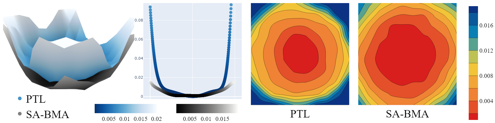
Figure 4: Comparison of the loss surfaces of SA-BMA (grey) and PTL (light blue) models. The loss surface comparison offers an intuitive view of SA-BMA achieving a lower, flatter loss surface than PTL, underlining the importance of flatness in model design.

5.3 Flatness Analysis

To substantiate the flatness in the loss surface of the SA-BMA model, we compare the sampled models from the posterior approximated with SA-BMA and PTL. The backbone model is RN18, and the trained dataset is CIFAR10 10-shot. As shown in Figure 4, we compare the sampled weight of SA-BMA and PTL in diverse views. All sceneries show SA-BMA converging to a flatter loss basin with lower loss. Additional results with more samples and the protocol to visualize the loss basin are provided in Appendix F.

We analyze beyond simply demonstrating the flatness of SA-BMA through illustrations by quantitatively comparing the sharpness of models. Table 4 presents the results of analyzing the eigenvalue of model Hessian for both DNN and BNN series baseline models, as well as SA-BMA. $\lambda_{1}$ and $\lambda_{5}$ represent the largest eigenvalue and the fifth largest eigenvalue, respectively. We used the maximal eigenvalue $\lambda_{1}$ and ratio $\lambda_{1}/\lambda_{5}$ as a metric [37, 76, 24]. SA-BMA has the lowest value compared to all other baselines, which can be interpreted as our model being the flattest. It further corroborates our visual findings, underscoring the superior flatness and, by extension, the enhanced generalization potential of the SA-BMA.

6 Related Works

6.1 Flatness and BNN

Recent works have suggested flat-seeking optimizers combined with BNN. First, SWAG [35] implicitly approximated posterior toward flatter optima based on SWA [77]. However, SWAG can fail to find flat minima, leading to limited improvement in generalization, as shown in Section 3.1. bSAM [25] showed that SAM can be interpreted as a relaxation of the Bayes and quantified uncertainty with SAM. Yet, bSAM only focused on uncertainty quantification by simply modifying Adam-based SAM [78], not newly considering the parametric geometry for perturbation. Moreover, scaling the variance with the number of data points hampers the direct implementation of bSAM in few-shot settings. Flat seeking BNN [60] proposed sharpness-aware likelihood and proved the effectiveness both experimentally and theoretically. They just employ the DNN-grounded SAM into BNN without considering the difference between nature of DNN and BNN. On the other hand, E-MCMC [24] proposed an efficient MCMC algorithm capable of effectively sampling the posterior within a flat basin by removing the nested chain of Entropy-SGD and Entropy-SGLD. Still, E-MCMC necessitates a guidance model, which doubles the parameters and heavily hinders its employment over large-scale models. SA-BMA is the first to reflect the parameter space in the perturbation step of SAM for stochastic models, considering the nature of BNNs.

6.2 Bayesian Transfer Learning

There are several works on performing transfer learning on BNN with prior. PTL [15] constructs BNN by learning closed-form posterior approximation of the pre-trained model on the source task and uses it as a prior for the downstream task after scaling. The work requires additional training on the source task, which makes it restrictive when it is impossible to access to the source task dataset. MOPED [61] employs pre-trained BNN as a prior for VI based on the empirical Bayes method. Using pre-trained DNN, MOPED enhances accessibility to BNN, however, it is only applicable to Mean-field VI (MFVI). Non-parametric transfer learning (NPTL) [79] suggested adopting non-parametric learning to make posterior flexible in terms of distribution shift. Our proposed scheme for Bayesian transfer learning can approximate the distribution of parameters within either the downstream dataset or the source dataset, which allows us to leverage more sophisticated and large-scale pre-trained models. Moreover, it is the first study considering flatness in Bayesian transfer learning.

7 Conclusion

This study shows that BNN can fail to capture the loss geometry well alone, and flatness affects the performance of BMA. As a result, we observe that the limited performance of BNN can be derived from the sharp posterior. To alleviate the problem, we propose a new optimization method for the flat posterior with the consideration of loss curvature. We validate that SA-BMA intrigues that BNN has a flat posterior as well as a generalization performance on diverse transfer learning and distribution shift. As training normalization and last layer only to avoid computational inability, SA-BMA is an efficient transfer learning method for BNN with significantly less training time. We believe it is a fascinating way to calculate the exact FIM for full-parameter feasible and optimize the whole model into flat mode.

Appendix A Additional Results For Flatness Dose Matter For Bayesian Model Averaging

A.1 Flatness Comparison

To prove that BNN cannot guarantee flatness, we run a variety experiments for flatness comparison. Since it’s uncommon, we do not run DNN or VI with SWAG learning rate scheduler for additional flatness comparisons. First, Table 5 summarizes the comparison results covering different models with a wide range of combinations with learning methods, optimizers, and schedulers. We conducte on RN18 w/o BN and data augmentation. We use MOPED as the VI framework.

Table 5: Flatness Comparison on DNN and BNN with sharpness-aware optimization methods. We observe that BNN does not find the flatness-aware local minima, and the compatibility of BNN and the previous sharpness-aware optimization (SAM) is limited. All experiments were repeated three times with RN18 w/o BN.

DataSet CIFAR10 CIFAR100 Methods Optim Schedule ACC $\uparrow$ ECE $\downarrow$ NLL $\downarrow$ $\lambda_{1}$ $\downarrow$ $\lambda_{1}/\lambda_{5}$ $\downarrow$ ACC $\uparrow$ ECE $\downarrow$ NLL $\downarrow$ $\lambda_{1}$ $\downarrow$ $\lambda_{1}/\lambda_{5}$ $\downarrow$ DNN SGD Constant $81.96_{\pm 0.55}$ $0.033_{\pm 0.004}$ $0.546_{\pm 0.015}$ $37.34_{\pm 3.59}$ $1.727_{\pm 0.229}$ $44.31_{\pm 1.02}$ $0.047_{\pm 0.004}$ $2.194_{\pm 0.032}$ $12.65_{\pm 0.87}$ $1.681_{\pm 0.172}$ Cos Decay $84.51_{\pm 0.53}$ $0.027_{\pm 0.015}$ $0.474_{\pm 0.030}$ $19.98_{\pm 2.64}$ $1.593_{\pm 0.097}$ $47.01_{\pm 0.52}$ $0.074_{\pm 0.004}$ $2.077_{\pm 0.027}$ $102.21_{\pm 12.42}$ $1.737_{\pm 0.097}$ SWAG lr $82.72_{\pm 3.08}$ $0.029_{\pm 0.023}$ $0.520_{\pm 0.097}$ $18.09_{\pm 6.97}$ $1.577_{\pm 0.068}$ $33.13_{\pm 1.12}$ $0.065_{\pm 0.010}$ $2.485_{\pm 0.362}$ $26.85_{\pm 2.04}$ $1.903_{\pm 0.107}$ SAM Constant $85.06_{\pm 0.68}$ $0.019_{\pm 0.006}$ $0.450_{\pm 0.019}$ $11.81_{\pm 0.50}$ $1.306_{\pm 0.020}$ $51.28_{\pm 0.32}$ $0.043_{\pm 0.018}$ $1.864_{\pm 0.014}$ $6.55_{\pm 0.16}$ $1.454_{\pm 0.061}$ Cos Decay $87.29_{\pm 0.12}$ $0.019_{\pm 0.003}$ $0.390_{\pm 0.004}$ $11.71_{\pm 0.24}$ $1.425_{\pm 0.006}$ $54.85_{\pm 0.62}$ $0.031_{\pm 0.006}$ $1.731_{\pm 0.007}$ $6.67_{\pm 0.61}$ $1.436_{\pm 0.026}$ SWAG lr $85.34_{\pm 2.76}$ $0.034_{\pm 0.015}$ $0.465_{\pm 0.057}$ $5.57_{\pm 0.58}$ $1.485_{\pm 0.053}$ $48.65_{\pm 1.44}$ $0.053_{\pm 0.012}$ $1.970_{\pm 0.065}$ $7.84_{\pm 0.04}$ $1.453_{\pm 0.013}$ SWAG SGD Constant $85.81_{\pm 0.42}$ $0.027_{\pm 0.007}$ $0.426_{\pm 0.005}$ $55.01_{\pm 4.74}$ $1.676_{\pm 0.004}$ $50.35_{\pm 0.40}$ $0.069_{\pm 0.031}$ $2.219_{\pm 0.067}$ $66.59_{\pm 20.34}$ $1.501_{\pm 0.048}$ Cos Decay $87.34_{\pm 0.48}$ $0.029_{\pm 0.006}$ $0.384_{\pm 0.013}$ $29.87_{\pm 2.55}$ $1.627_{\pm 0.024}$ $52.31_{\pm 0.81}$ $0.101_{\pm 0.065}$ $2.132_{\pm 0.166}$ $24.58_{\pm 15.13}$ $1.529_{\pm 0.062}$ SWAG lr $86.07_{\pm 0.12}$ $0.113_{\pm 0.115}$ $0.435_{\pm 0.002}$ $50.88_{\pm 3.00}$ $1.665_{\pm 0.022}$ $51.52_{\pm 0.40}$ $0.124_{\pm 0.008}$ $2.237_{\pm 0.175}$ $44.21_{\pm 5.79}$ $1.654_{\pm 0.010}$ SAM Constant $85.40_{\pm 0.28}$ $0.015_{\pm 0.003}$ $0.437_{\pm 0.010}$ $17.67_{\pm 0.60}$ $1.451_{\pm 0.016}$ $50.01_{\pm 0.93}$ $0.102_{\pm 0.044}$ $2.143_{\pm 0.143}$ $15.86_{\pm 6.91}$ $1.354_{\pm 0.042}$ Cos Decay $87.01_{\pm 0.09}$ $0.014_{\pm 0.002}$ $0.391_{\pm 0.005}$ $9.90_{\pm 0.60}$ $1.426_{\pm 0.026}$ $52.53_{\pm 0.31}$ $0.070_{\pm 0.002}$ $1.973_{\pm 0.019}$ $13.92_{\pm 0.38}$ $1.412_{\pm 0.005}$ SWAG lr $86.39_{\pm 0.36}$ $0.022_{\pm 0.005}$ $0.417_{\pm 0.008}$ $11.17_{\pm 0.85}$ $1.443_{\pm 0.020}$ $52.35_{\pm 0.16}$ $0.098_{\pm 0.008}$ $2.021_{\pm 0.015}$ $12.92_{\pm 1.27}$ $1.406_{\pm 0.020}$ VI SGD Constant $83.11_{\pm 0.40}$ $0.016_{\pm 0.002}$ $0.518_{\pm 0.011}$ $19.72_{\pm 0.88}$ $1.49_{\pm 0.049}$ $45.81_{\pm 0.42}$ $0.018_{\pm 0.002}$ $2.104_{\pm 0.017}$ $217.05_{\pm 16.11}$ $1.67_{\pm 0.083}$ Cos Decay $84.51_{\pm 0.30}$ $0.037_{\pm 0.003}$ $0.465_{\pm 0.005}$ $20.86_{\pm 0.58}$ $1.53_{\pm 0.015}$ $48.30_{\pm 0.41}$ $0.121_{\pm 0.007}$ $2.519_{\pm 0.029}$ $34.71_{\pm 2.06}$ $1.80_{\pm 0.095}$ SAM Constant $83.25_{\pm 0.34}$ $0.016_{\pm 0.003}$ $0.502_{\pm 0.007}$ $10.74_{\pm 0.74}$ $1.46_{\pm 0.072}$ $45.67_{\pm 0.60}$ $0.119_{\pm 0.003}$ $2.436_{\pm 0.065}$ $33.54_{\pm 0.33}$ $1.70_{\pm 0.120}$ Cos Decay $84.34_{\pm 0.35}$ $0.024_{\pm 0.001}$ $0.494_{\pm 0.003}$ $24.63_{\pm 0.83}$ $1.42_{\pm 0.040}$ $48.51_{\pm 0.71}$ $0.121_{\pm 0.004}$ $2.516_{\pm 0.061}$ $33.49_{\pm 1.99}$ $1.76_{\pm 0.021}$

Second, we compare the flatness with ResNet18 pre-trained on ImageNet 1K, provided in torchvision. Note that the ResNet18 contains Batch Normalization, and data augmentation is also applied in this setting. Table 6 consistently shows the SWAG cannot guarantee the flatness with Batch Normalization and data augmentation, either. One compelling point is naive SAM can make the model generalize better by adding normalization layers. In line with [80] and [48], it shows the power of normalization layers and its effect on SAM.

Table 6: Flatness Comparison on DNN and BNN with sharpness-aware optimization methods. We observe that BNN does not find the flatness-aware local minima even with BN and data augmentation. All experiments were repeated three times with ResNet18 pre-trained on ImageNet 1K.

DataSet CIFAR10 CIFAR100 Methods Optim Schedule ACC $\uparrow$ ECE $\downarrow$ NLL $\downarrow$ $\lambda_{1}$ $\downarrow$ $\lambda_{1}/\lambda_{5}$ $\downarrow$ ACC $\uparrow$ ECE $\downarrow$ NLL $\downarrow$ $\lambda_{1}$ $\downarrow$ $\lambda_{1}/\lambda_{5}$ $\downarrow$ DNN SGD Constant $95.60_{\pm 0.21}$ $0.005_{\pm 0.001}$ $0.127_{\pm 0.002}$ $587.06_{\pm 17.13}$ $2.22_{\pm 0.065}$ $80.61_{\pm 0.17}$ $0.059_{\pm 0.005}$ $0.674_{\pm 0.003}$ $1261.65_{\pm 44.00}$ $1.97_{\pm 0.005}$ Cos Decay $96.46_{\pm 0.08}$ $0.010_{\pm 0.001}$ $0.110_{\pm 0.001}$ $436.79_{\pm 22.52}$ $2.07_{\pm 0.276}$ $82.00_{\pm 0.40}$ $0.058_{\pm 0.001}$ $0.656_{\pm 0.007}$ $1195.30_{\pm 33.53}$ $2.35_{\pm 0.086}$ SAM Constant $96.55_{\pm 0.11}$ $0.005_{\pm 0.002}$ $0.102_{\pm 0.001}$ $115.97_{\pm 6.09}$ $1.92_{\pm 0.074}$ $82.06_{\pm 0.40}$ $0.040_{\pm 0.004}$ $0.617_{\pm 0.005}$ $306.44_{\pm 43.19}$ $2.19_{\pm 0.190}$ Cos Decay $96.92_{\pm 0.14}$ $0.031_{\pm 0.002}$ $0.112_{\pm 0.002}$ $728.99_{\pm 5.07}$ $2.06_{\pm 0.053}$ $83.76_{\pm 0.13}$ $0.060_{\pm 0.001}$ $0.589_{\pm 0.003}$ $382.66_{\pm 10.00}$ $2.07_{\pm 0.052}$ SWAG SGD Constant $96.46_{\pm 0.06}$ $0.084_{\pm 0.026}$ $0.178_{\pm 0.031}$ $2263.44_{\pm 1025.76}$ $2.86_{\pm 0.886}$ $82.99_{\pm 0.20}$ $0.118_{\pm 0.016}$ $0.677_{\pm 0.022}$ $2227.27_{\pm 539.94}$ $3.00_{\pm 0.510}$ Cos Decay $96.54_{\pm 0.09}$ $0.021_{\pm 0.001}$ $0.116_{\pm 0.002}$ $1147.92_{\pm 165.90}$ $2.74_{\pm 0.357}$ $82.48_{\pm 0.22}$ $0.083_{\pm 0.001}$ $0.667_{\pm 0.006}$ $2457.46_{\pm 224.32}$ $2.93_{\pm 0.086}$ SWAG lr $96.35_{\pm 0.10}$ $0.090_{\pm 0.011}$ $0.192_{\pm 0.015}$ $7823.13_{\pm 2183.11}$ $3.03_{\pm 0.362}$ $82.34_{\pm 0.19}$ $0.052_{\pm 0.002}$ $0.638_{\pm 0.003}$ $1529.73_{\pm 58.99}$ $3.02_{\pm 0.102}$ SAM Constant $96.94_{\pm 0.04}$ $0.014_{\pm 0.001}$ $0.096_{\pm 0.002}$ $564.11_{\pm 242.04}$ $2.72_{\pm 0.203}$ $83.55_{\pm 0.25}$ $0.099_{\pm 0.005}$ $0.629_{\pm 0.010}$ $1158.40_{\pm 187.01}$ $2.91_{\pm 0.193}$ Cos Decay $97.10_{\pm 0.02}$ $0.012_{\pm 0.001}$ $0.090_{\pm 0.001}$ $206.03_{\pm 21.85}$ $1.98_{\pm 0.022}$ $83.73_{\pm 0.22}$ $0.065_{\pm 0.003}$ $0.852_{\pm 0.006}$ $687.73_{\pm 93.92}$ $2.31_{\pm 0.132}$ SWAG lr $97.03_{\pm 0.03}$ $0.006_{\pm 0.001}$ $0.090_{\pm 0.000}$ $123.84_{\pm 6.00}$ $2.04_{\pm 0.067}$ $83.63_{\pm 0.16}$ $0.061_{\pm 0.002}$ $0.581_{\pm 0.005}$ $501.41_{\pm 36.32}$ $2.15_{\pm 0.072}$

Third, we train the pre-trained ResNet18 with CIFAR10 10-shot and CIFAR100 10-shot. In other words, we only use 10 data per class in this setting. Table 7 shows identical results with other flatness comparisons. First, SWAG cannot guarantee flatness without SAM. In the meantime, SAM helps SWAG to find flatter optima, but it is hard to ensure better generalization without exceptions.

Table 7: Flatness Comparison on DNN and BNN with sharpness-aware optimization method. We observe that BNN does not find the flatness-aware local minima, and the compatibility of BNN and the previous sharpness-aware optimization (SAM) is limited. All experiments were repeated three times with ResNet18 pre-trained ImageNet 1K in few-shot setting.

DataSet CIFAR10 10-shot CIFAR100 10-shot Methods Optim Schedule ACC $\uparrow$ ECE $\downarrow$ NLL $\downarrow$ $\lambda_{1}$ $\downarrow$ $\lambda_{1}/\lambda_{5}$ $\downarrow$ ACC $\uparrow$ ECE $\downarrow$ NLL $\downarrow$ $\lambda_{1}$ $\downarrow$ $\lambda_{1}/\lambda_{5}$ $\downarrow$ DNN SGD Constant $81.96_{\pm 0.55}$ $0.033_{\pm 0.004}$ $0.546_{\pm 0.015}$ $37.34_{\pm 3.59}$ $1.73_{\pm 0.229}$ $44.31_{\pm 1.02}$ $0.047_{\pm 0.004}$ $2.194_{\pm 0.032}$ $12.65_{\pm 0.87}$ $1.68_{\pm 0.172}$ Cos Decay $84.51_{\pm 0.53}$ $0.027_{\pm 0.015}$ $0.474_{\pm 0.030}$ $19.98_{\pm 2.64}$ $1.59_{\pm 0.097}$ $47.01_{\pm 0.52}$ $0.074_{\pm 0.004}$ $2.077_{\pm 0.027}$ $102.21_{\pm 12.42}$ $1.74_{\pm 0.097}$ SAM Constant $57.91_{\pm 1.84}$ $0.030_{\pm 0.017}$ $1.227_{\pm 0.038}$ $199.79_{\pm 47.69}$ $2.25_{\pm 0.426}$ $45.54_{\pm 0.64}$ $0.094_{\pm 0.011}$ $2.118_{\pm 0.021}$ $359.59_{\pm 38.51}$ $1.86_{\pm 0.049}$ Cos Decay $56.54_{\pm 2.57}$ $0.015_{\pm 0.005}$ $1.255_{\pm 0.070}$ $148.59_{\pm 17.70}$ $2.12_{\pm 0.190}$ $45.51_{\pm 1.26}$ $0.106_{\pm 0.009}$ $2.131_{\pm 0.051}$ $426.73_{\pm 51.64}$ $2.08_{\pm 0.293}$ SWAG SGD Constant $55.74_{\pm 1.57}$ $0.018_{\pm 0.002}$ $1.289_{\pm 0.047}$ $530.71_{\pm 48.39}$ $1.53_{\pm 0.314}$ $44.22_{\pm 1.27}$ $0.120_{\pm 0.003}$ $2.221_{\pm 0.069}$ $976.07_{\pm 178.03}$ $2.42_{\pm 0.276}$ Cos Decay $56.47_{\pm 0.77}$ $0.042_{\pm 0.013}$ $1.274_{\pm 0.036}$ $566.26_{\pm 96.65}$ $2.18_{\pm 0.329}$ $44.18_{\pm 1.26}$ $0.102_{\pm 0.009}$ $2.225_{\pm 0.051}$ $588.19_{\pm 70.21}$ $2.46_{\pm 0.293}$ SWAG lr $56.13_{\pm 1.37}$ $0.041_{\pm 0.007}$ $1.272_{\pm 0.059}$ $562.87_{\pm 116.08}$ $2.16_{\pm 0.373}$ $43.91_{\pm 1.00}$ $0.106_{\pm 0.004}$ $2.214_{\pm 0.058}$ $756.86_{\pm 68.28}$ $2.10_{\pm 0.160}$ SAM Constant $57.96_{\pm 2.04}$ $0.031_{\pm 0.003}$ $1.229_{\pm 0.047}$ $229.31_{\pm 36.64}$ $2.31_{\pm 0.134}$ $46.48_{\pm 0.67}$ $0.115_{\pm 0.005}$ $2.106_{\pm 0.021}$ $536.30_{\pm 13.45}$ $2.10_{\pm 0.108}$ Cos Decay $57.61_{\pm 1.27}$ $0.047_{\pm 0.004}$ $1.231_{\pm 0.036}$ $351.87_{\pm 49.76}$ $2.35_{\pm 0.508}$ $46.10_{\pm 0.44}$ $0.118_{\pm 0.001}$ $2.150_{\pm 0.013}$ $490.13_{\pm 57.45}$ $2.01_{\pm 0.163}$ SWAG lr $56.62_{\pm 1.96}$ $0.014_{\pm 0.002}$ $1.269_{\pm 0.049}$ $175.89_{\pm 20.77}$ $2.11_{\pm 0.212}$ $45.02_{\pm 0.31}$ $0.082_{\pm 0.004}$ $2.160_{\pm 0.035}$ $220.03_{\pm 6.49}$ $1.93_{\pm 0.055}$

Fourth, we measure the flatness of last-layer SWAG (L-SWAG) and VI (L-VI) at Table 8. We use the trained DNN models as an initial weight for L-SWAG. For example, a DNN model trained with constant lr scheduling and SGD optimizer is the base model for L-SWAG, which trains with the same lr schedule and optimizer. For L-VI, we only set stochastic parameters for last layer. We affirm that employing SAM only on the last layer barely influences the flatness and generalization, or has restrictive impact.

Table 8: Flatness Comparison on DNN and L-SWAG applied to the DNN. We confirm that using pre-existed flatness-aware optimization on the last layer of BNN cannot be enough to pull the model to a flat basin. All experiments were repeated three times with ResNet18 w/o BN.

DataSet CIFAR10 CIFAR100 Methods Optim Schedule ACC $\uparrow$ ECE $\downarrow$ NLL $\downarrow$ $\lambda_{1}$ $\downarrow$ $\lambda_{1}/\lambda_{5}$ $\downarrow$ ACC $\uparrow$ ECE $\downarrow$ NLL $\downarrow$ $\lambda_{1}$ $\downarrow$ $\lambda_{1}/\lambda_{5}$ $\downarrow$ DNN SGD Constant $81.96_{\pm 0.55}$ $0.033_{\pm 0.004}$ $0.546_{\pm 0.015}$ $37.34_{\pm 3.59}$ $1.73_{\pm 0.229}$ $44.31_{\pm 1.02}$ $0.047_{\pm 0.004}$ $2.194_{\pm 0.032}$ $12.65_{\pm 0.87}$ $1.68_{\pm 0.172}$ Cos Decay $84.51_{\pm 0.53}$ $0.027_{\pm 0.015}$ $0.474_{\pm 0.030}$ $19.98_{\pm 2.64}$ $1.59_{\pm 0.097}$ $47.01_{\pm 0.52}$ $0.074_{\pm 0.004}$ $2.077_{\pm 0.027}$ $102.21_{\pm 12.42}$ $1.74_{\pm 0.097}$ SWAG lr $82.72_{\pm 3.08}$ $0.029_{\pm 0.023}$ $0.520_{\pm 0.097}$ $18.09_{\pm 6.97}$ $1.57_{\pm 0.068}$ $33.13_{\pm 1.12}$ $0.065_{\pm 0.010}$ $2.485_{\pm 0.362}$ $26.85_{\pm 2.04}$ $1.90_{\pm 0.107}$ SAM Constant $85.06_{\pm 0.68}$ $0.019_{\pm 0.006}$ $0.450_{\pm 0.019}$ $11.81_{\pm 0.50}$ $1.31_{\pm 0.020}$ $51.28_{\pm 0.32}$ $0.043_{\pm 0.018}$ $1.864_{\pm 0.014}$ $6.55_{\pm 0.16}$ $1.45_{\pm 0.061}$ Cos Decay $87.29_{\pm 0.12}$ $0.019_{\pm 0.003}$ $0.390_{\pm 0.004}$ $11.71_{\pm 0.24}$ $1.43_{\pm 0.006}$ $54.85_{\pm 0.62}$ $0.031_{\pm 0.006}$ $1.731_{\pm 0.007}$ $6.67_{\pm 0.61}$ $1.44_{\pm 0.026}$ SWAG lr $85.34_{\pm 2.76}$ $0.034_{\pm 0.015}$ $0.465_{\pm 0.057}$ $5.57_{\pm 0.58}$ $1.49_{\pm 0.053}$ $48.65_{\pm 1.44}$ $0.053_{\pm 0.012}$ $1.970_{\pm 0.065}$ $7.84_{\pm 0.04}$ $1.45_{\pm 0.013}$ L-SWAG SGD Constant $82.20_{\pm 0.40}$ $0.036_{\pm 0.007}$ $0.544_{\pm 0.007}$ $49.49_{\pm 4.71}$ $1.68_{\pm 0.080}$ $49.65_{\pm 0.65}$ $0.053_{\pm 0.003}$ $1.980_{\pm 0.012}$ $18.65_{\pm 1.14}$ $1.71_{\pm 0.134}$ Cos Decay $84.94_{\pm 0.70}$ $0.034_{\pm 0.01}$ $0.475_{\pm 0.012}$ $26.26_{\pm 2.81}$ $1.62_{\pm 0.055}$ $49.56_{\pm 0.58}$ $0.015_{\pm 0.003}$ $1.938_{\pm 0.014}$ $131.32_{\pm 13.82}$ $1.65_{\pm 0.046}$ SWAG lr $83.26_{\pm 3.10}$ $0.043_{\pm 0.027}$ $0.544_{\pm 0.052}$ $49.49_{\pm 8.86}$ $1.68_{\pm 0.134}$ $49.65_{\pm 0.65}$ $0.053_{\pm 0.002}$ $1.980_{\pm 0.036}$ $18.65_{\pm 3.26}$ $1.71_{\pm 0.021}$ SAM Constant $82.19_{\pm 0.38}$ $0.037_{\pm 0.007}$ $0.544_{\pm 0.007}$ $49.50_{\pm 4.74}$ $1.69_{\pm 0.085}$ $49.44_{\pm 0.59}$ $0.055_{\pm 0.004}$ $1.991_{\pm 0.012}$ $18.76_{\pm 1.36}$ $1.72_{\pm 0.146}$ Cos Decay $84.95_{\pm 0.69}$ $0.035_{\pm 0.016}$ $0.4762_{\pm 0.010}$ $26.47_{\pm 2.96}$ $1.63_{\pm 0.058}$ $49.39_{\pm 0.50}$ $0.025_{\pm 0.001}$ $1.963_{\pm 0.015}$ $140.33_{\pm 15.64}$ $1.66_{\pm 0.042}$ SWAG lr $83.27_{\pm 3.09}$ $0.043_{\pm 0.027}$ $0.539_{\pm 0.051}$ $23.28_{\pm 9.31}$ $1.63_{\pm 0.134}$ $39.35_{\pm 0.61}$ $0.157_{\pm 0.210}$ $2.374_{\pm 0.036}$ $38.85_{\pm 3.19}$ $1.76_{\pm 0.154}$ L-VI SGD Constant $83.46_{\pm 0.34}$ $0.027_{\pm 0.002}$ $0.529_{\pm 0.000}$ $29.65_{\pm 3.44}$ $1.64_{\pm 0.087}$ $49.26_{\pm 0.69}$ $0.046_{\pm 0.006}$ $2.068_{\pm 0.018}$ $63.17_{\pm 7.96}$ $1.61_{\pm 0.165}$ Cos Decay $85.11_{\pm 0.35}$ $0.083_{\pm 0.003}$ $0.605_{\pm 0.007}$ $55.92_{\pm 3.02}$ $1.56_{\pm 0.076}$ $50.70_{\pm 2.29}$ $0.130_{\pm 0.083}$ $2.424_{\pm 0.337}$ $47.53_{\pm 38.46}$ $1.61_{\pm 0.24}$ SAM Constant $84.49_{\pm 1.19}$ $0.025_{\pm 0.007}$ $0.484_{\pm 0.034}$ $11.78_{\pm 0.21}$ $1.46_{\pm 0.038}$ $51.13_{\pm 0.13}$ $0.058_{\pm 0.008}$ $2.135_{\pm 0.141}$ $22.80_{\pm 3.51}$ $1.50_{\pm 0.067}$ Cos Decay $85.94_{\pm 0.25}$ $0.021_{\pm 0.002}$ $0.439_{\pm 0.002}$ $14.91_{\pm 0.38}$ $1.34_{\pm 0.044}$ $54.04_{\pm 0.68}$ $0.087_{\pm 0.005}$ $2.063_{\pm 0.009}$ $26.35_{\pm 1.86}$ $1.42_{\pm 0.055}$

Figure 5: Comparison of Error, NLL, and ECE with various schedulers on CIFAR10 in relation to the maximum eigenvalue $\lambda_{1}$.

Figure 6: Comparison of Error, NLL, and ECE with various schedulers on CIFAR100 in relation to the maximum eigenvalue $\lambda_{1}$.

In Figure 1, only the Error and NLL in relation to the maximum eigenvalue $\lambda_{1}$ are presented for training with the Constant scheduler. Figures 5 and 6 show the Error, NLL, and additionally ECE with various schedulers and datasets. These figures depict the experimental results on CIFAR10 and CIFAR100, respectively. Similar to what was observed in Figure 1, BNN does not guarantee model flatness, and using SAM instead of SGD in BNN provides a limited improvement in generalization performance despite leveraging flatness.

A.2 Correlation Between Flatness and Generalization

Together with flatness comparisons in A.1, we check the correlation between flatness and generalization performance of sampled models throughout all considered learning rate schedulers. We present the scatter plot of the model, sampled from Resnet18 w/o BN trained on CIFAR10 and CIFAR100 in the first and second rows of Figure 7. Each column of Figure 7 denotes Constant scheduler, Cosine Decay scheduler, and SWAG lr scheduler, respectively. All the models are trained with SWAG and SGD momentum, and we set maximal eigenvalue $\lambda_{1}$ as a flatness measure. Correlation with flatness and each generalization performance metric is suggested in the legend, as well. Regardless of the scheduler and dataset, all generalization performances, error, ECE, and NLL strongly correlate with flatness.

(a) Constant scheduler

(b) Cosine Decay scheduler

(c) SWAG lr scheduler

(d) Constant scheduler

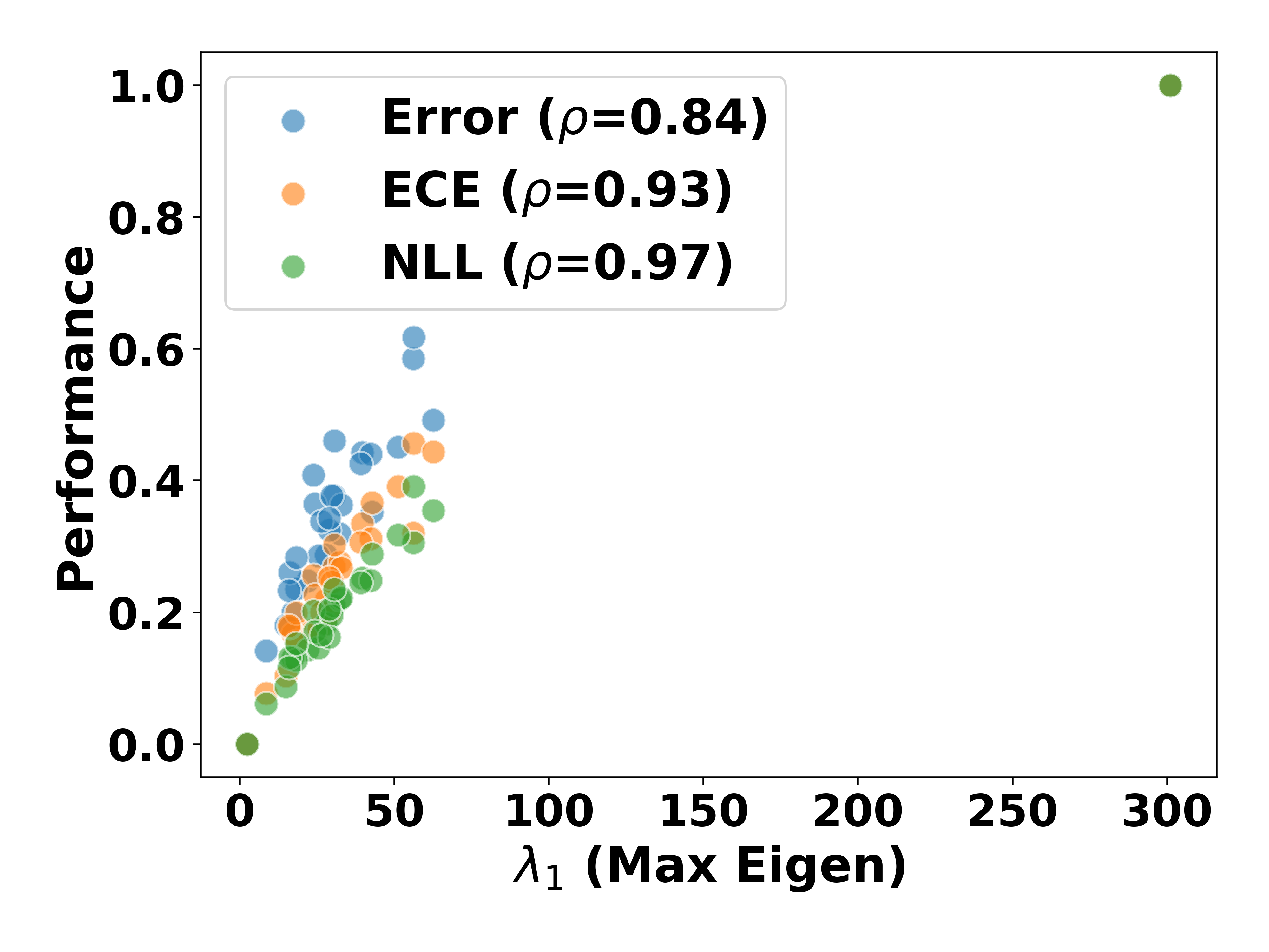
(e) Cosine Decay scheduler

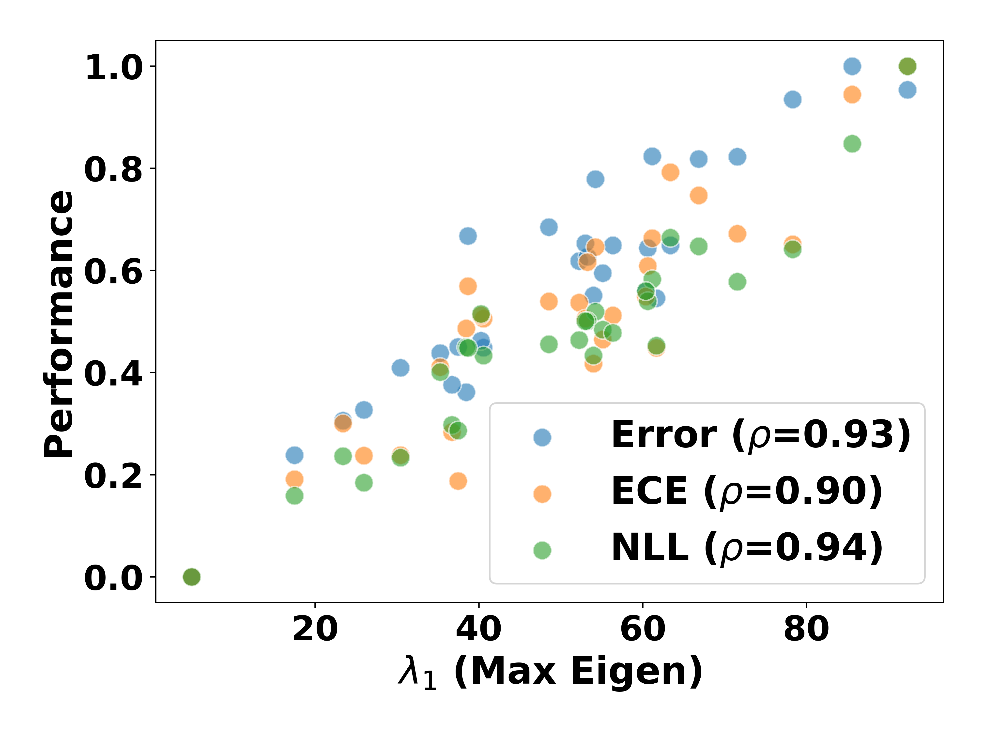
(f) SWAG lr scheduler

Figure 7: Correlation between maximal eigenvalue and performances of 30 sampled models from SWAG throughout all considered schedulers. It shows classification error, ECE, and NLL are distinctly correlated with flatness. We conjecture that the flatness is crucial for the generalization performance of BNN

A.3 Progressive BMA Based On Flatness

We also inspect the influence of flatness on BMA performance throughout all considered schedulers. We prepared 30 sampled models, trained on CIFAR10 and CIFAR100 with ResNet18 w/o BN. "Flat" denotes starting BMA from sampling the flattest model. "Sharp" denotes starting BMA by sampling the sharpest model. "Rand" denotes starting BMA from a random sample of prepared 30 models. Figure 8 and 9 shows the results in CIFAR10 and CIFAR100, respectively. Each row means Constant, Cosine Decay, and SWAG lr scheduler, and each column denotes the classification error, ECE, and NLL.

Generally, we observe that there is no significant improvement or limited improvement in performance when gradually applying BMA from flat models. Following from the observation, we conclude flatness should be taken into account for efficient BMA. This observation is particularly pronounced in classification error ((a), (d), (g) of Figure 8 and 9). However, the trend is inconsistent in ECE. It is an interesting topic for future research.

(a) Error

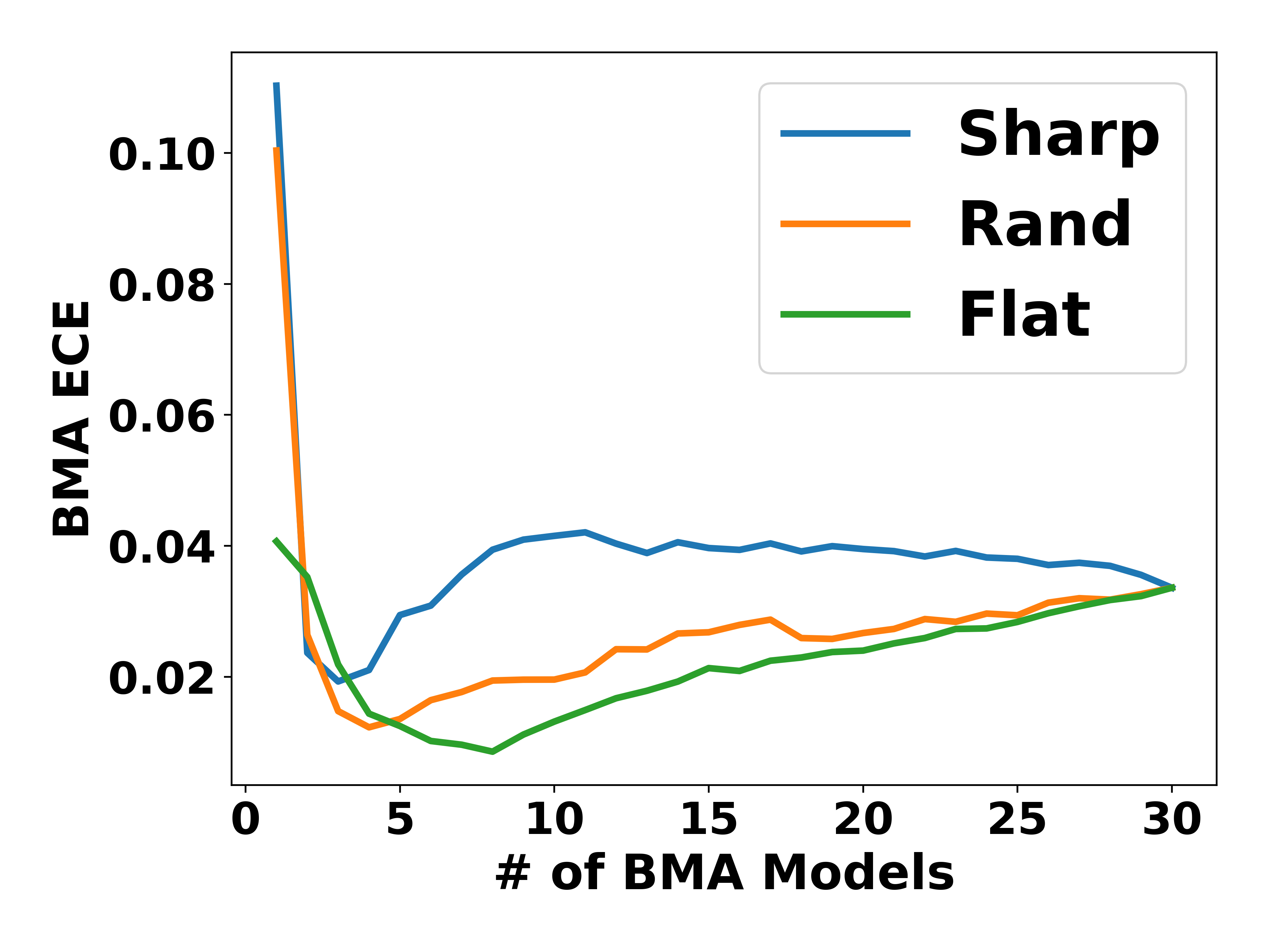
(b) ECE

(c) NLL

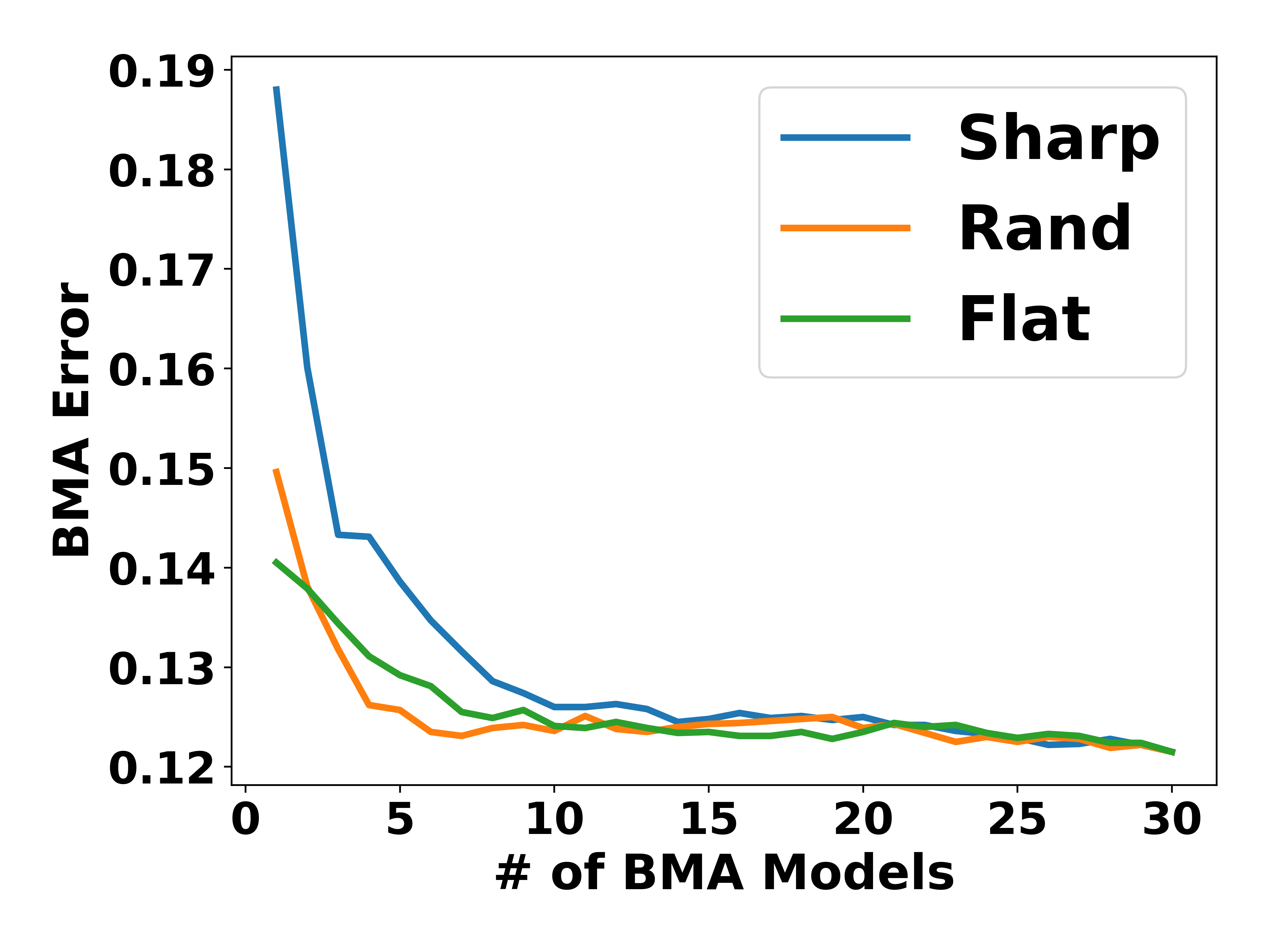
(d) Error

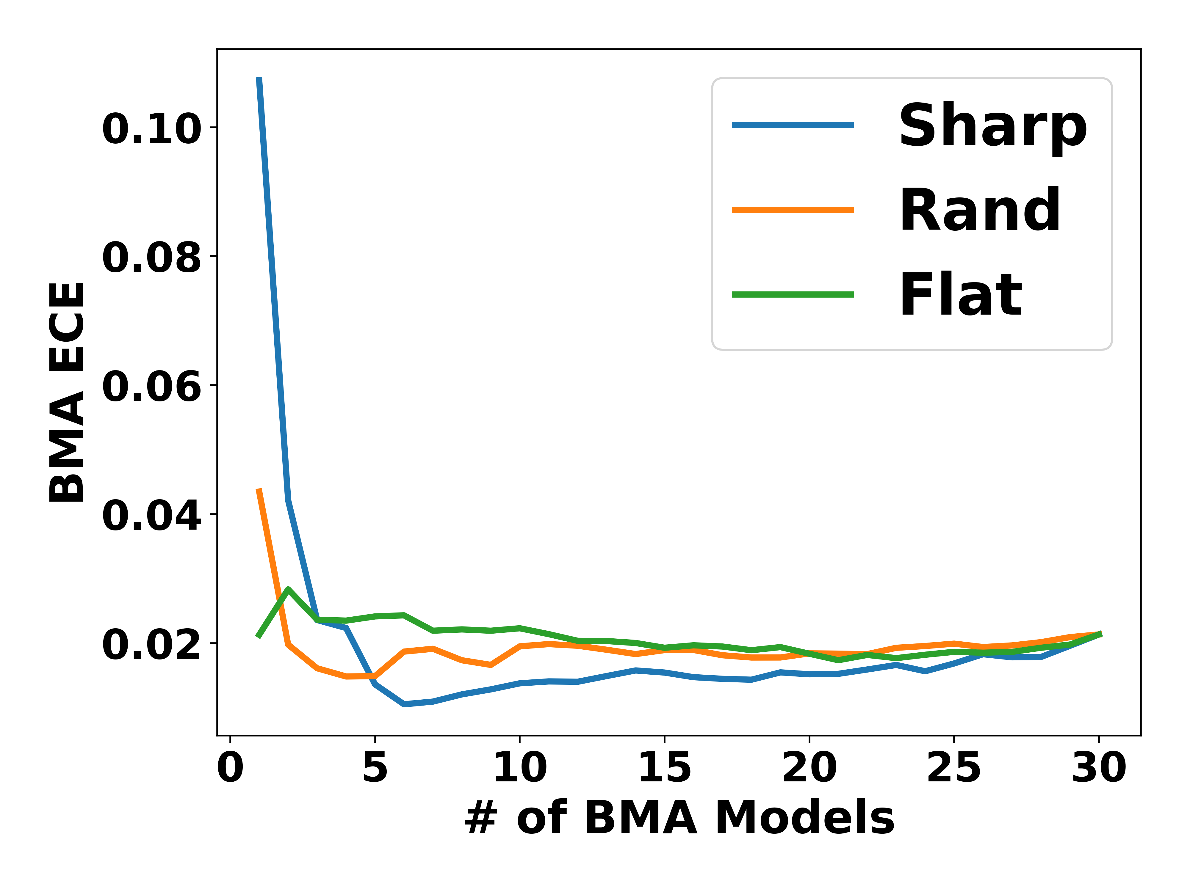
(e) ECE

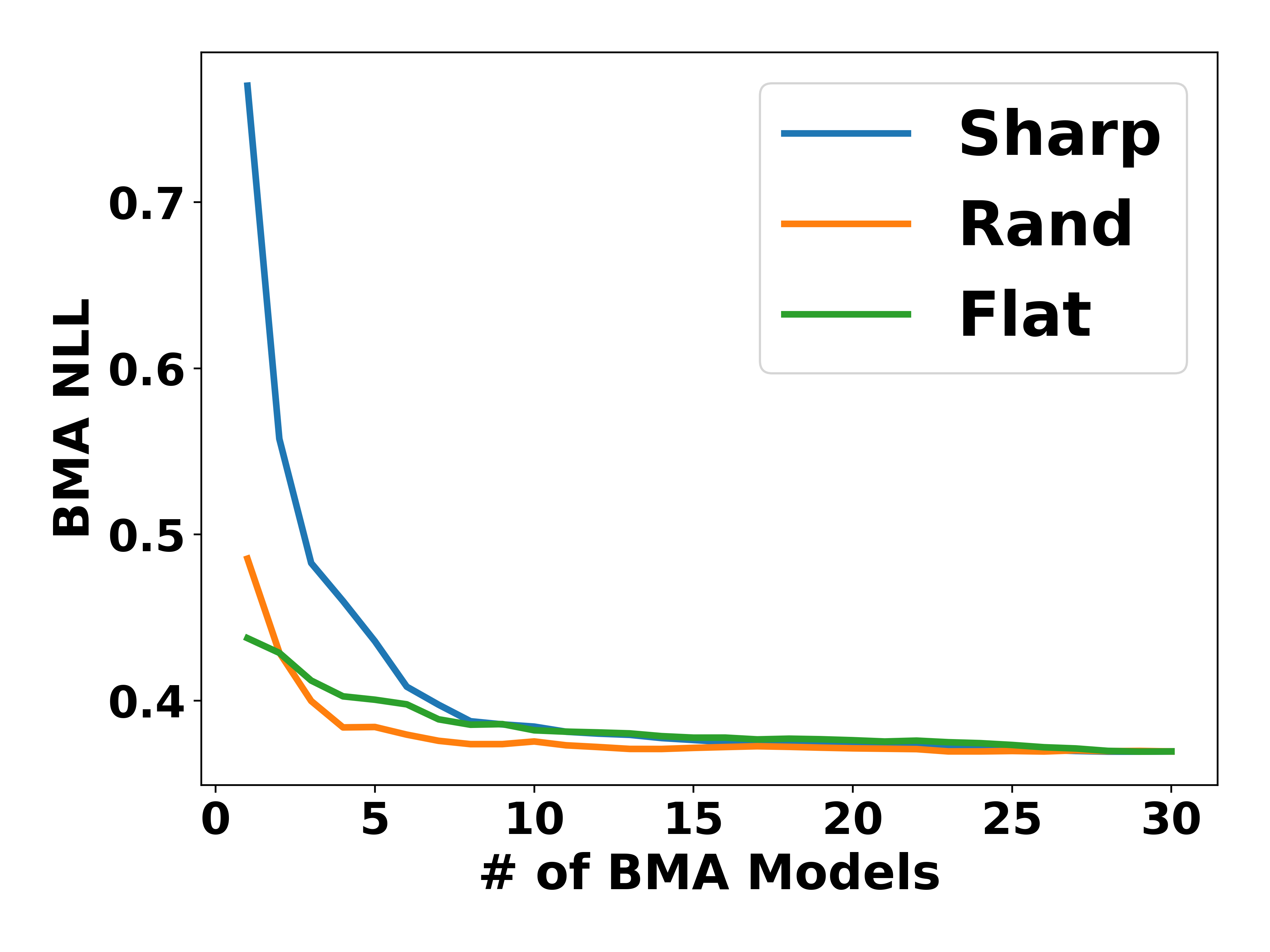
(f) NLL

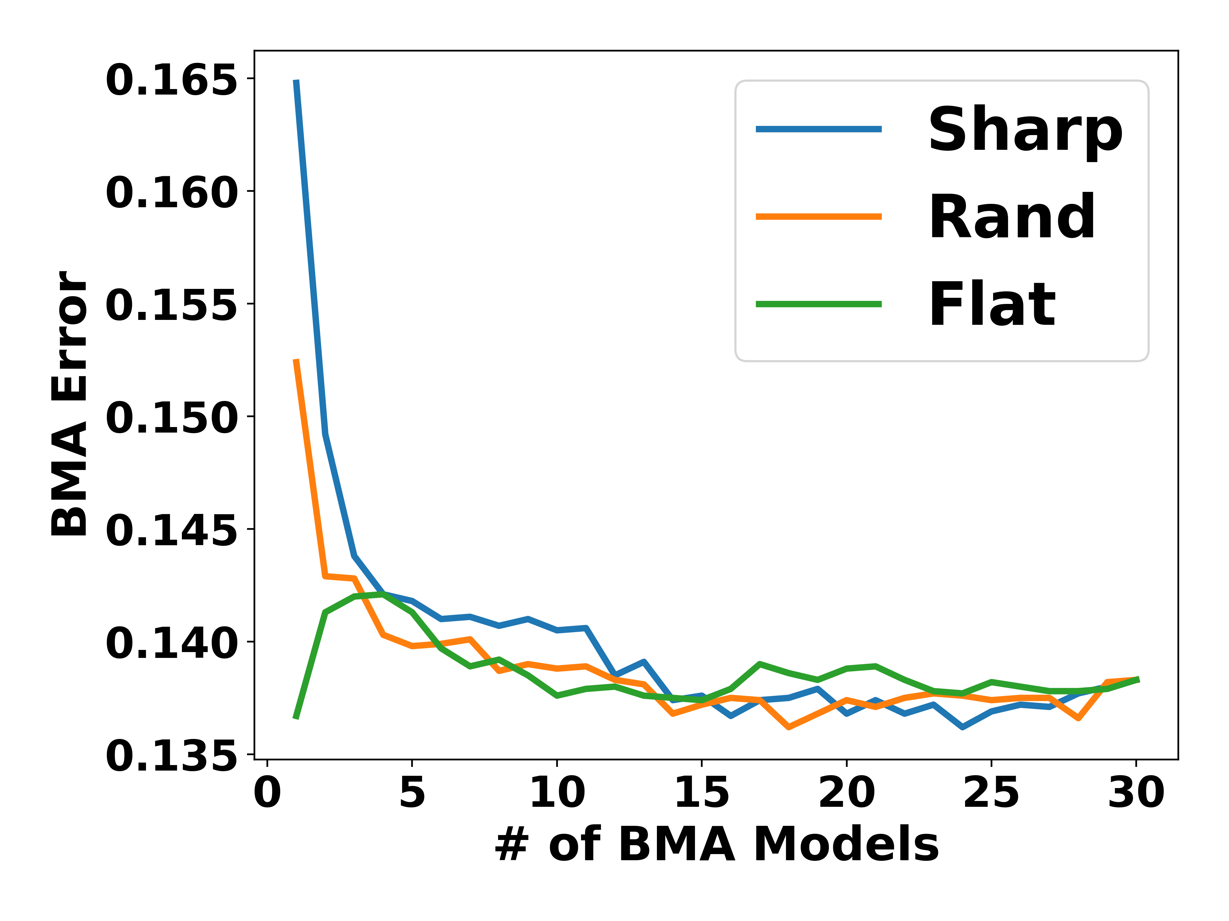
(g) Error

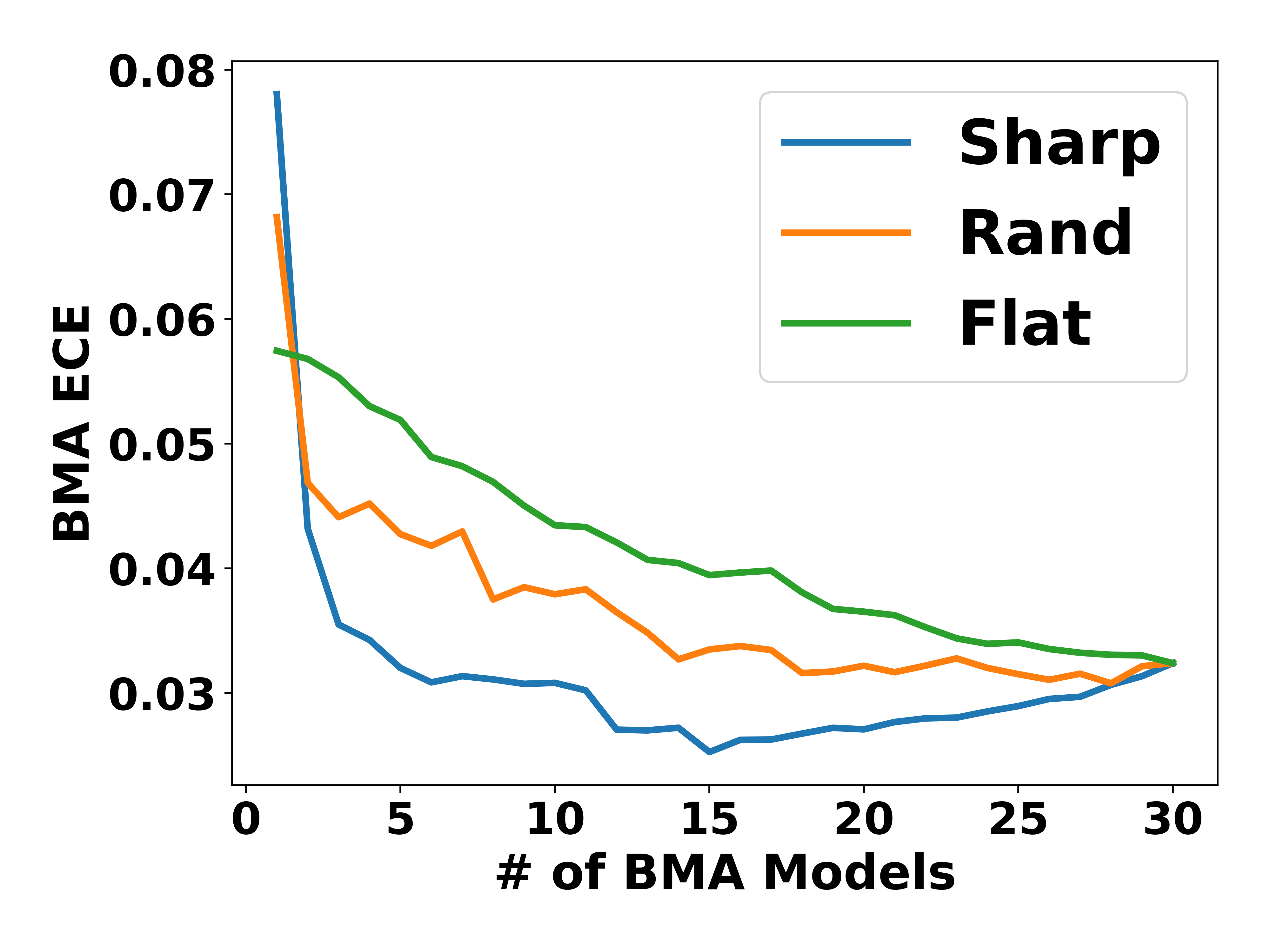
(h) ECE

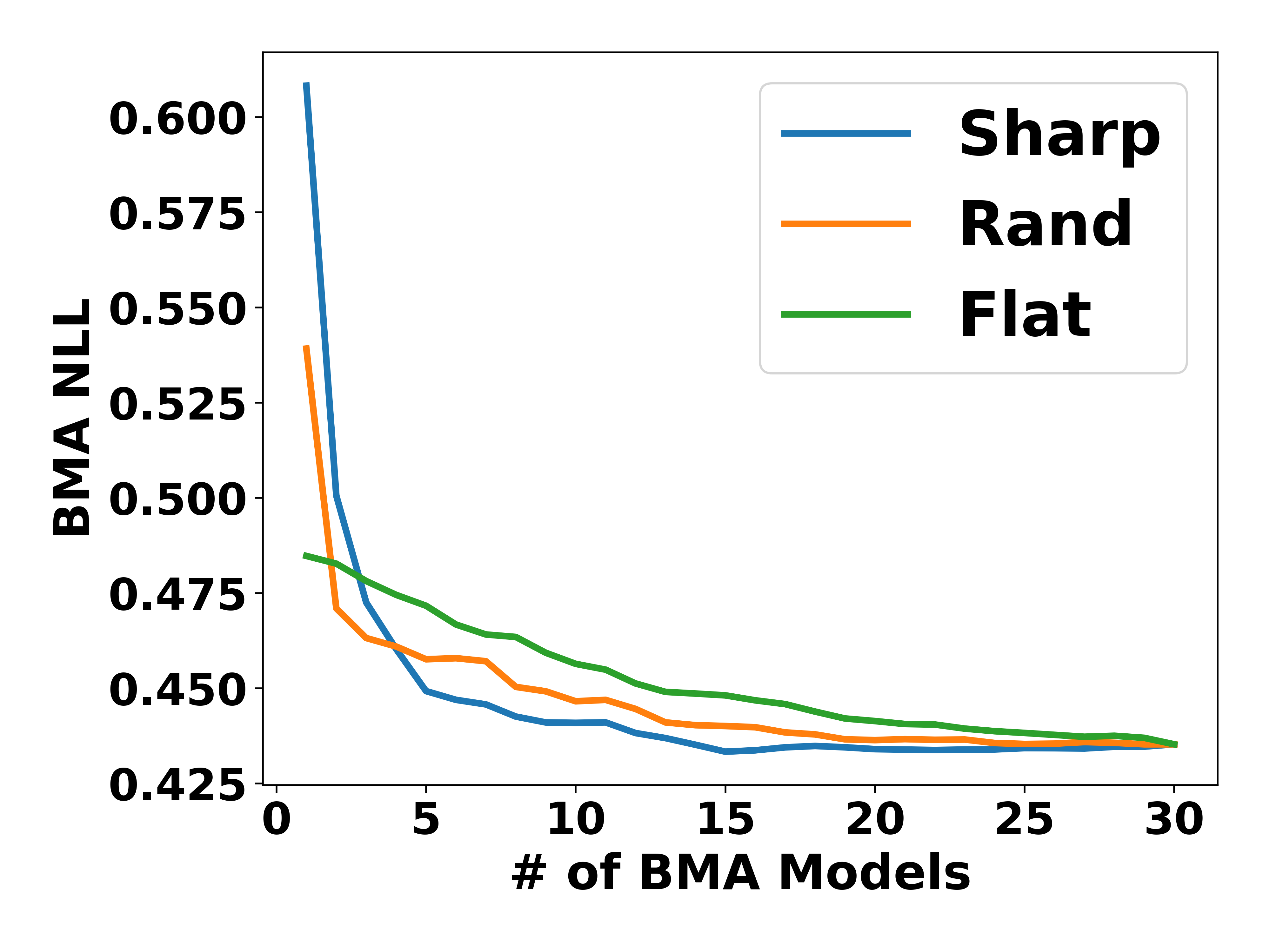
(i) NLL

Figure 8: Performance variation based on sampling considering flatness among BMA on CIFAR10. Each row means the Constant, Cos Decay, and SWAG lr scheduler. Each column denotes classification error, ECE, and NLL. "Flat" denotes starting BMA from sampling the flattest model, and "Sharp" means the opposite of "Flat". "Rand" denotes starting BMA from a random sample of prepared 30 models. It reveals that the flatness should be taken into account for efficient BMA.

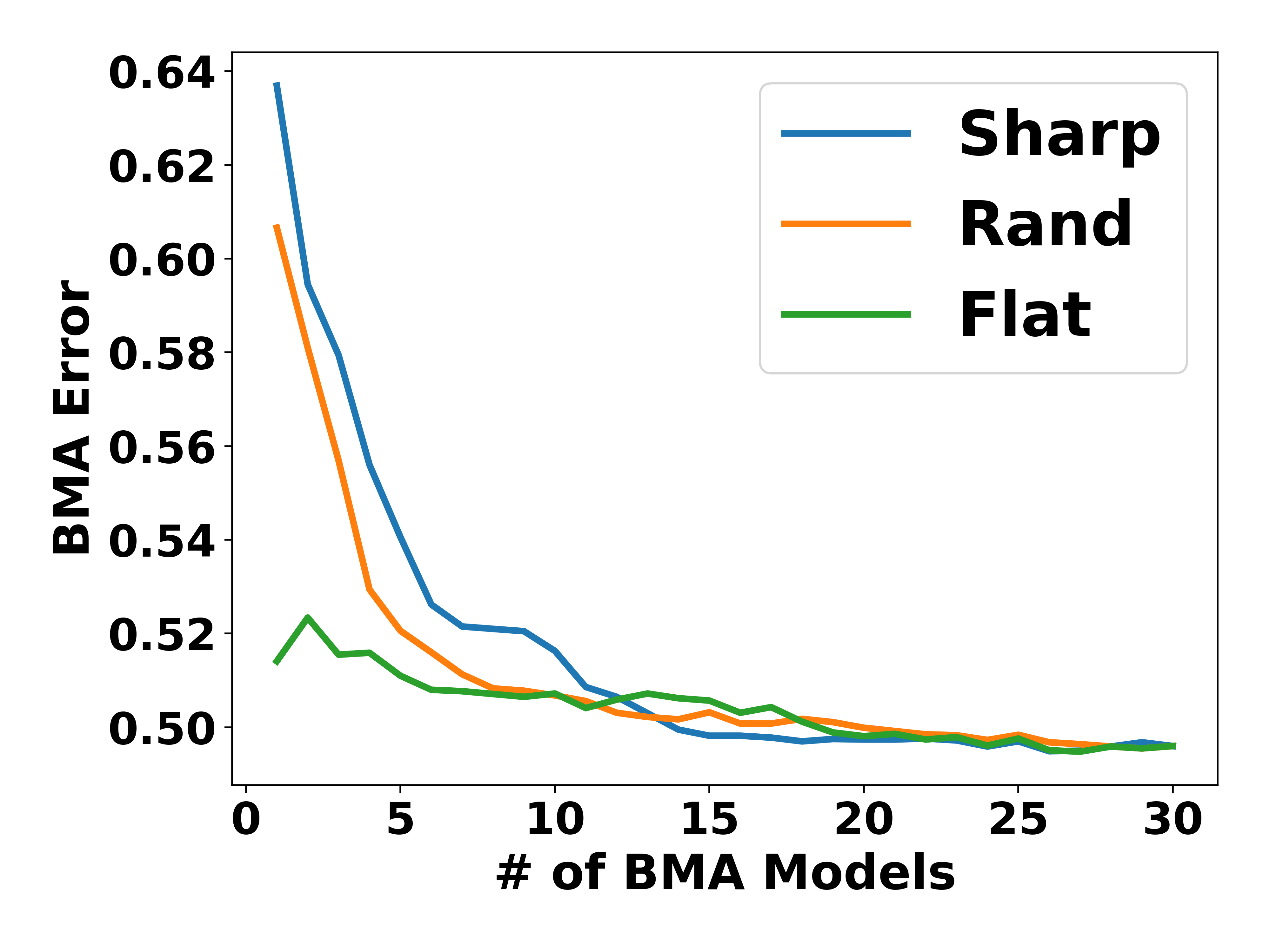
(a) Error

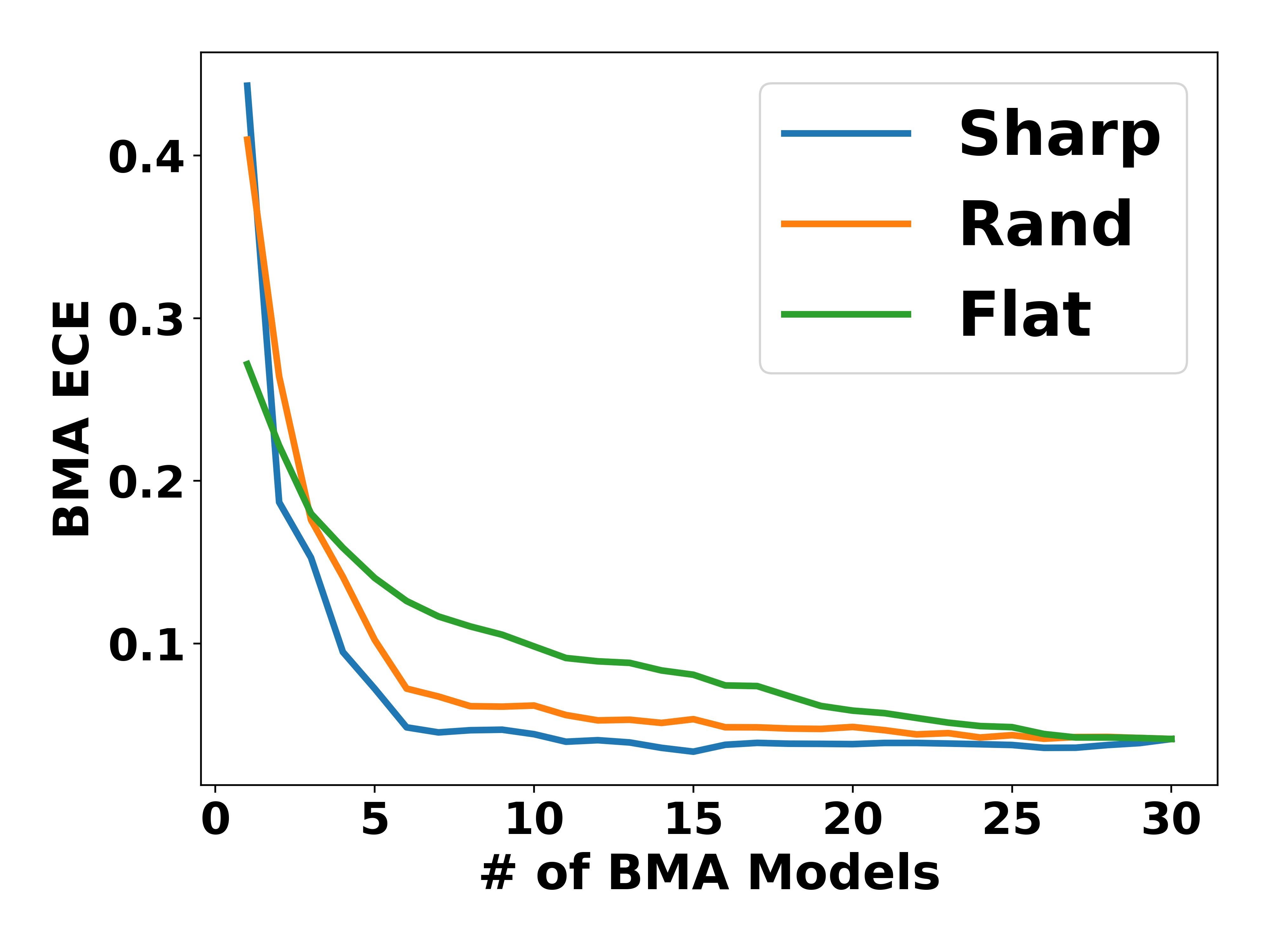
(b) ECE

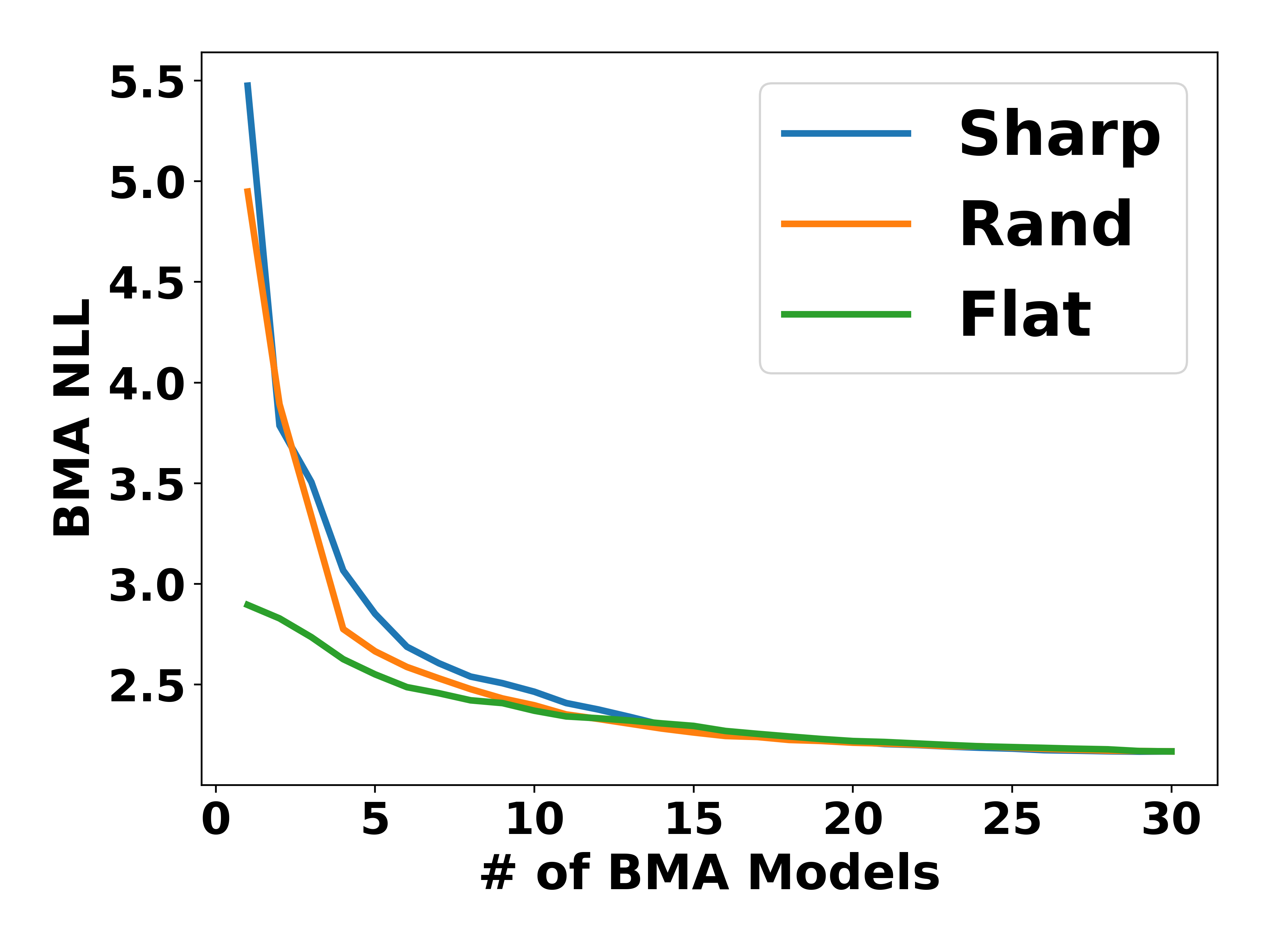
(c) NLL

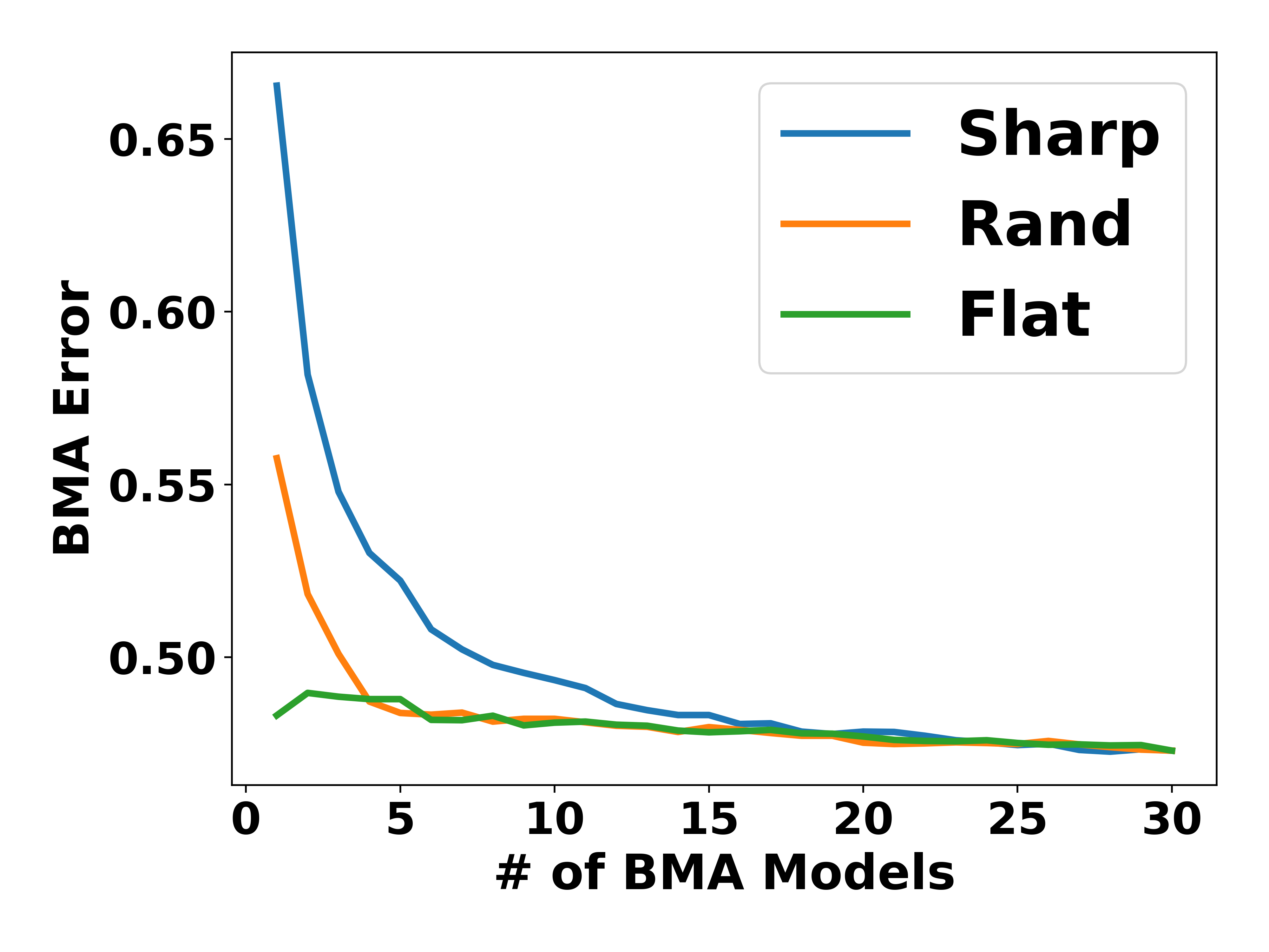
(d) Error

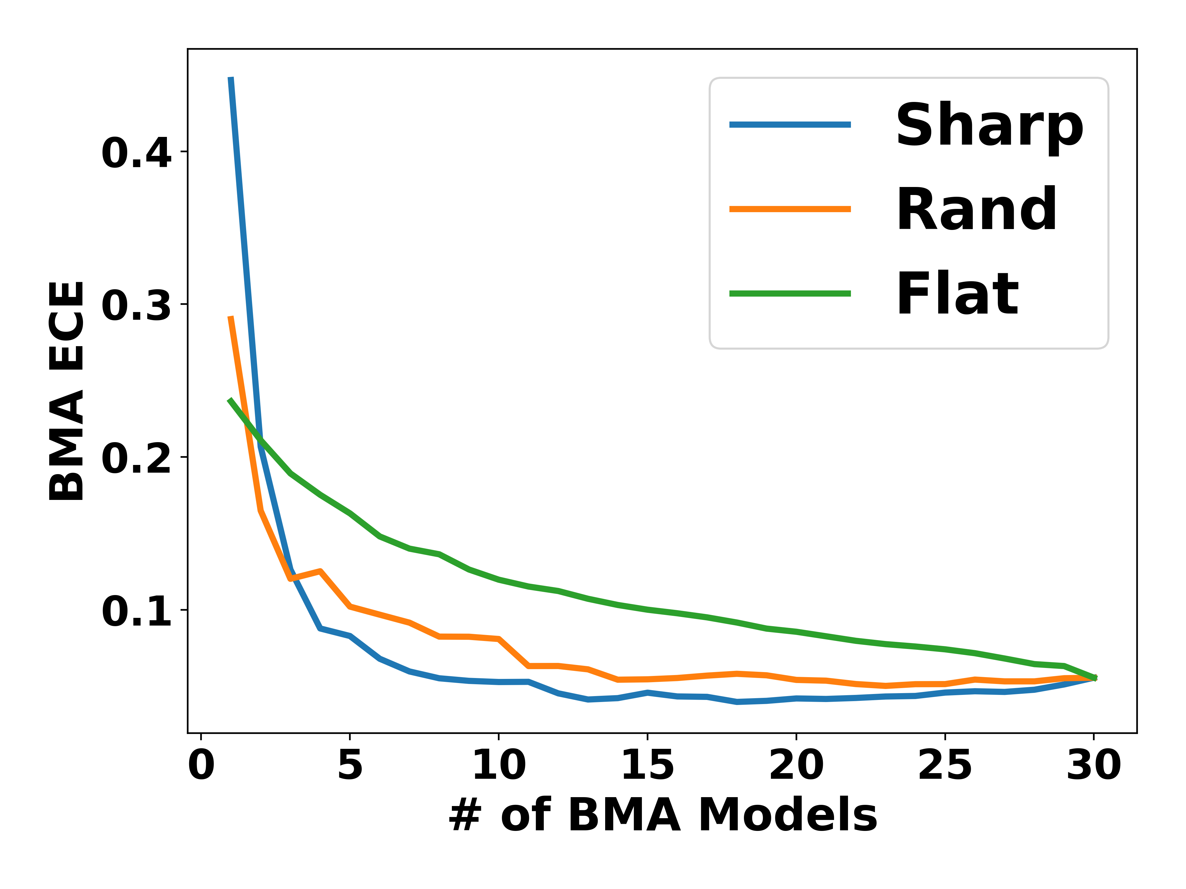
(e) ECE

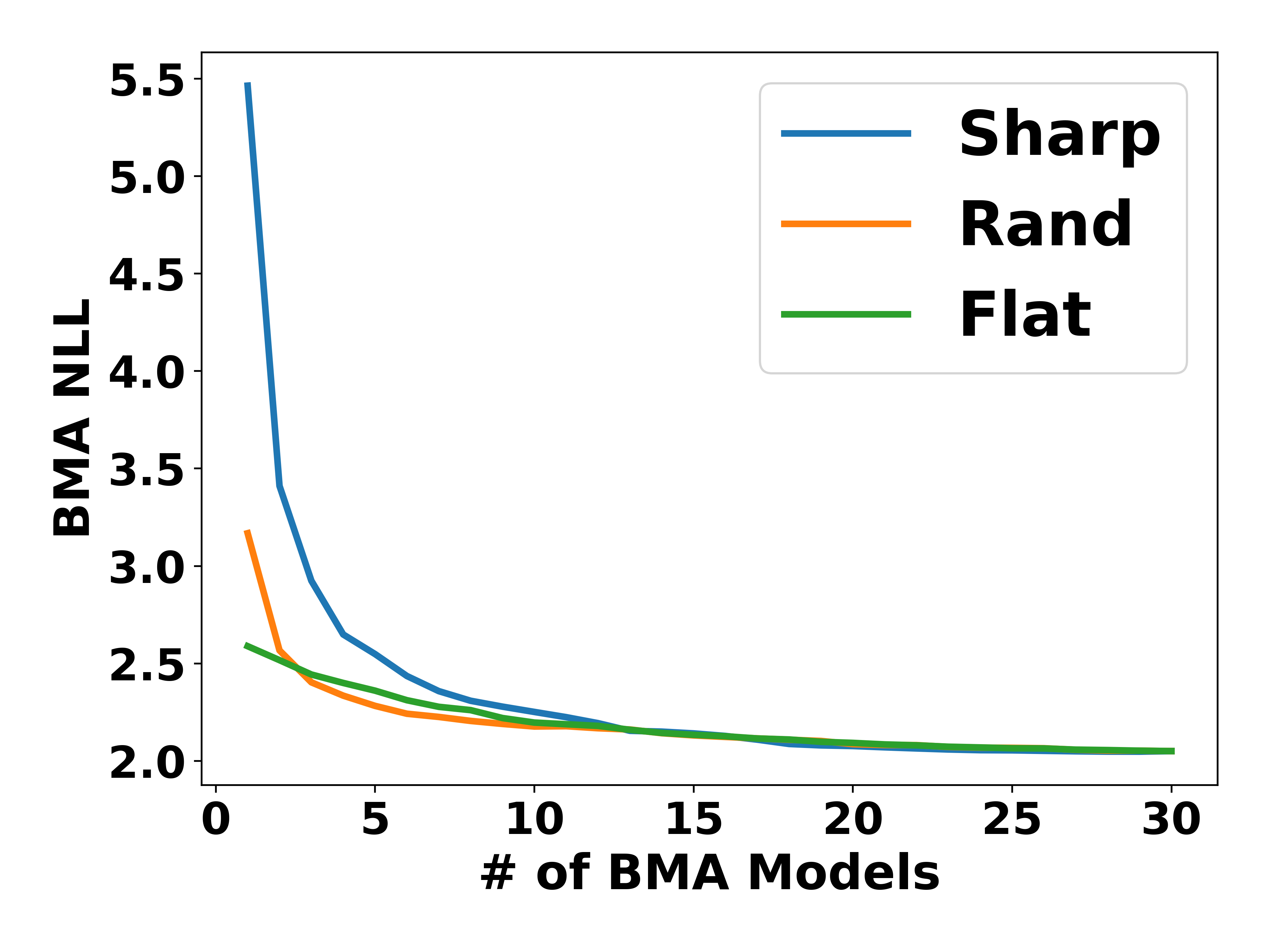
(f) NLL

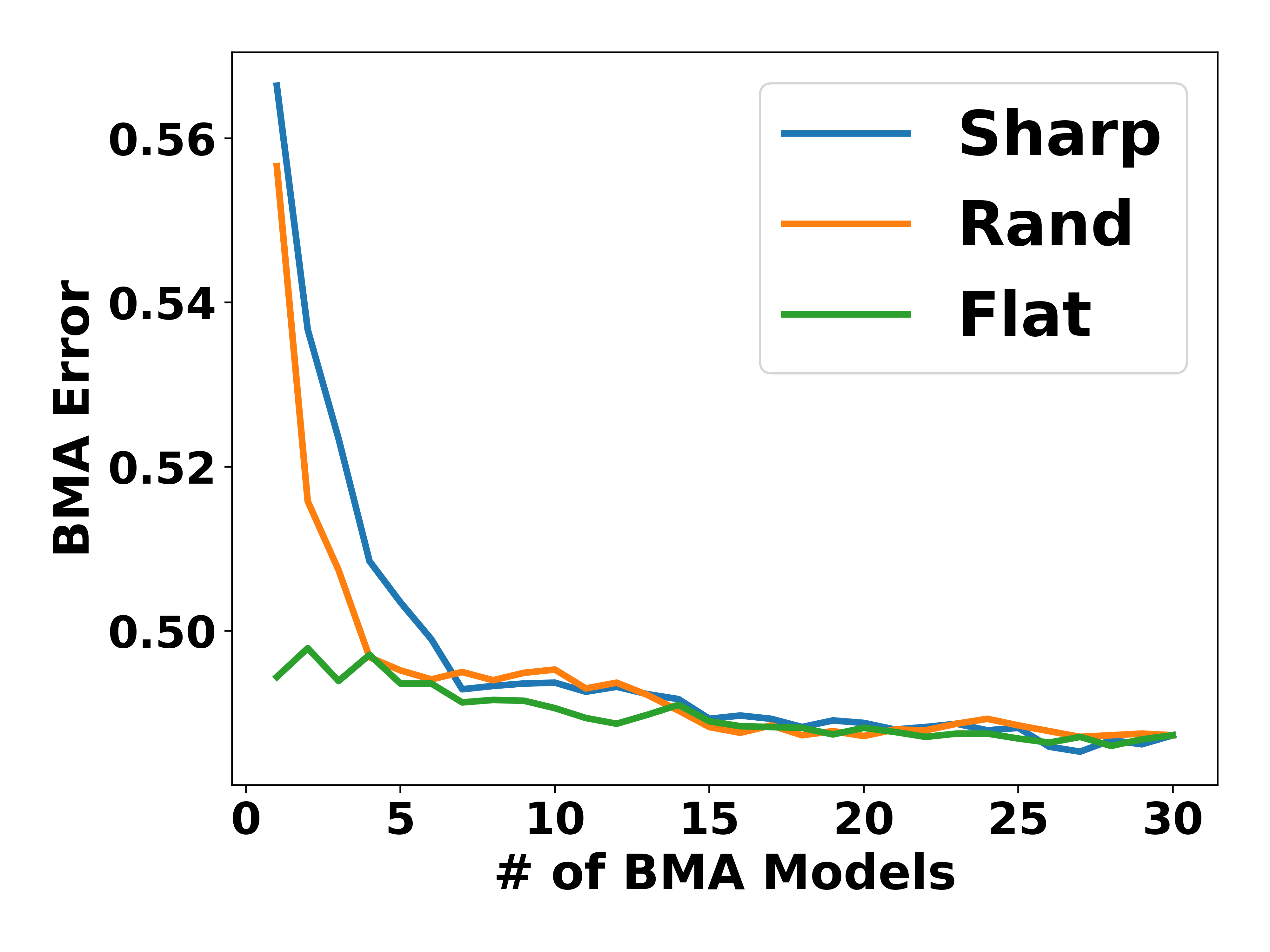
(g) Error

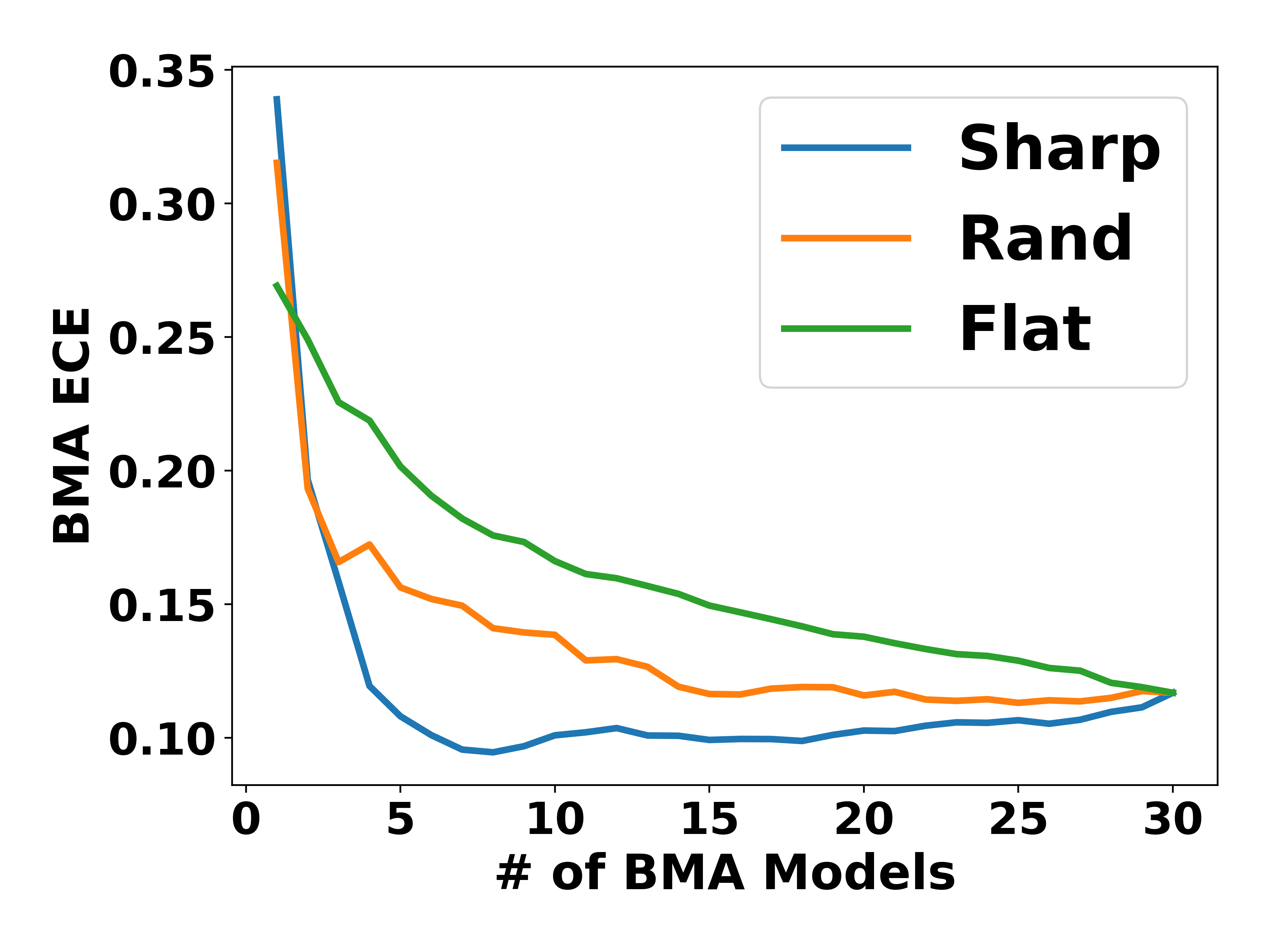
(h) ECE

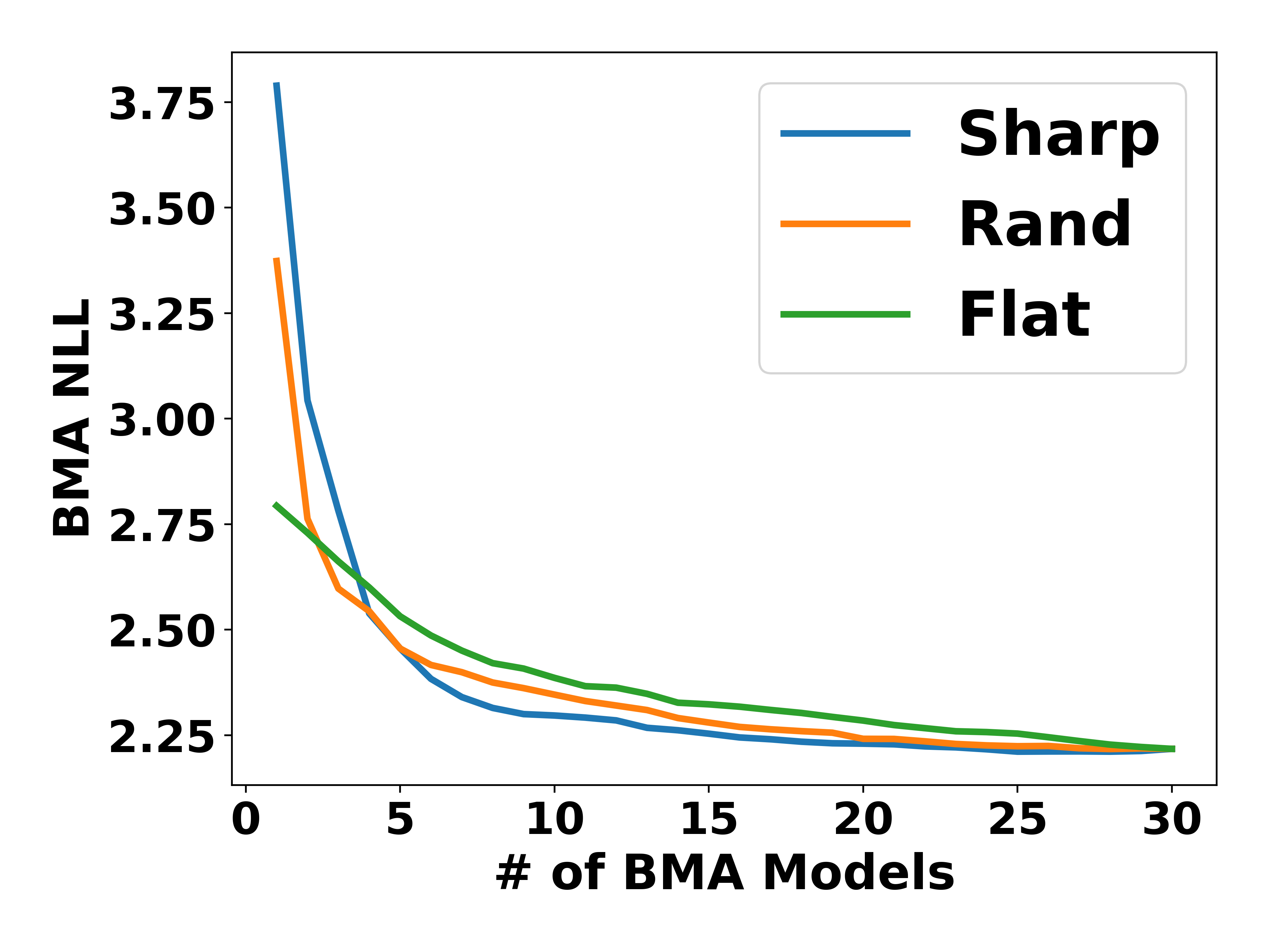
(i) NLL

Figure 9: Performance variation based on sampling considering flatness among BMA on CIFAR100. Each row means the Constant, Cos Decay, and SWAG lr scheduler. Each column denotes classification error, ECE, and NLL. "Flat" denotes starting BMA from sampling the flattest model, and "Sharp" means the opposite of "Flat". "Rand" denotes starting BMA from a random sample of prepared 30 models. It reveals that the flatness should be taken into account for efficient BMA.

Appendix B Experimental Details

B.1 Hyperparameters for Experiments

In this section, we provide the details of the experimental setup. First, we provide remarks for each baseline method, followed by the tables of hyperparameter configuration with respect to downstream datasets and the baselines. For all experiments, the hyperparameters are selected using grid-search. Configuration of best hyperparameters for each baseline is summarized in Table 9. We ran all experiments using GeForce RTX 3090 and NVIDIA RTX A6000 with GPU memory of 24,576MB and 49,140 MB.

Table 9: Hyperparameter Configuration

Dataset-Backbone Baseline learning rate $\beta_{1}$ (momentum) $\beta_{2}$ $\gamma$ weight decay CIFAR10 - ResNet18 SGD 5e-3 $\times$ $\times$ $\times$ 1e-3 SAM 1e-2 0.9 $\times$ 0.1 1e-4 SWAG-SGD 5e-3 0.9 $\times$ $\times$ 1e-5 SWAG-SAM 5e-3 0.9 $\times$ 5e-2 5e-4 bSAM 0.1 0.9 0.999 0.05 0.1 MOPED (SGD) 1e-2 0.9 $\times$ $\times$ 1e-4 EMCMC 5e-2 $\times$ $\times$ $\times$ 1e-3 PTL 0.1 $\times$ $\times$ $\times$ 1e-3 SA-BMA (Ours) 5e-2 0.9 $\times$ 0.1 5e-4 CIFAR10 - ViT-B/16 SGD 1e-3 0.9 $\times$ $\times$ 1e-4 SAM 1e-3 0.9 $\times$ 1e-2 1e-3 SWAG-SGD 1e-3 0.9 $\times$ $\times$ 1e-3 SWAG-SAM 1e-3 0.9 $\times$ 1e-2 1e-3 bSAM 0.1 0.9 0.999 1e-2 0.1 MOPED 1e-3 0.9 $\times$ $\times$ 1e-4 EMCMC 5e-3 $\times$ $\times$ $\times$ 1e-2 PTL 6e-2 $\times$ $\times$ $\times$ 1e-3 SA-BMA (Ours) 5e-3 0.9 $\times$ 0.5 5e-4 CIFAR100 - ResNet18 SGD 1e-2 0.9 $\times$ $\times$ 5e-3 SAM 1e-2 0.9 $\times$ 5e-2 1e-2 SWAG-SGD 1e-2 0.9 $\times$ $\times$ 1e-4 SWAG-SAM 1e-2 0.9 $\times$ 0.05 1e-2 bSAM 1 0.9 0.999 1e-2 1e-2 MOPED 1e-2 0.9 $\times$ $\times$ 1e-3 EMCMC 5e-2 $\times$ $\times$ $\times$ 1e-3 PTL 0.5 $\times$ $\times$ $\times$ 1e-3 SA-BMA (Ours) 5e-2 0.9 $\times$ 0.5 5e-4 CIFAR100 - ViT-B/16 SGD 1e-3 0.9 $\times$ $\times$ 1e-2 SAM 1e-3 0.9 $\times$ 1e-2 1e-2 SWAG-SGD 1e-3 0.9 $\times$ $\times$ 1e-2 SWAG-SAM 1e-3 0.9 $\times$ 1e-2 1e-2 bSAM 0.25 0.9 0.999 1e-2 1e-3 MOPED (SGD) 1e-3 0.9 $\times$ $\times$ 1e-3 EMCMC 5e-3 $\times$ $\times$ $\times$ 1e-3 PTL 0.1 $\times$ $\times$ $\times$ 1e-3 SA-BMA (Ours) 1e-2 0.9 $\times$ 0.5 5e-4

Stochastic Gradient Descent with Momentum (SGD)

In this study, we adopt Stochastic Gradient Descent with Momentum as an optimizer for DNN. Learning rate schedule is fixed to cosine decay with warmup length 10. We tested [100, 150] epoch and set 100 epoch as the best option. In overall experiments, we set momentum as 0.9. The hyperparameter tuning range included learning rate in [1e-4, 1e-3, 1e-2], weight decay in [1e-4, 5e-4, 1e-3, 1e-2].

Sharpness Aware Minimization (SAM)

We set SGD with momentum as the base optimizer of SAM. It also ran upon a cosine decay learning rate scheduler. All the range of hyperparameters is shared with SGD with Momenmtum. Additional hyperparameter $\gamma$, the ball size of perturbation, is in [1e-2, 5e-2, 0.1].

SAM as an optimal relaxation of Bayes (bSAM)

We use a cosine learning rate decay scheme, annealing the learning rate to zero. We fine-tuned pre-trained models for 150 epochs with fixed $\beta_{1}$ and $\beta_{2}$. The hyperparameter tuning rage included: learning rate in [1, 0.5, 0.25, 0.1, 5e-2, 1e-2, 1e-3], weight decay in [0.1, 1e-2, 1e-3], damping in [0.1, 1e-2, 1e-3], noise scaling parameter in [0.1, 1e-2, 1e-3, 1e-4], and $\gamma$ in [0.1, 5e-2, 1e-2, 1e-3]. Damping parameter stabilizes the method by adding constant when updating variance estimate. Since SAM as Bayes optimizer depends on the number of samples to scale the prior, we introduced additional noise scaling parameters to mitigate the gap between the experimental settings, where SAM as Bayes assumed training from scratch and our method assumed few-shot fine-tuning on the pre-trained model. We multiplied noise scaling parameter to the variance of the Gaussian noise to give strong prior, assuming pre-trained model.

Model Priors with Empirical Bayes using DNN (MOPED)

MOPED was a baseline to compare for Bayesian Transfer Learning. It employs pre-trained DNN and transforms it into Mean-Field Variational Inference (MFVI). We set prior mean and variance as 0 and 1, respectively. Besides, we set the posterior mean as 0 and variance as 1e-3. We adopt Reparameterization as type of VI. The essential hyperparmeter for MOPED is $\delta$, which adjust how much to incoroporate pre-trained weights. The $\delta$ was searched in [0.05, 0.1, 0.2, 0.3]. Moreover, we add a hyperparameter $\beta$ for MOPED that can balance the loss term in VI. The $\beta$ is in range [1e-2, 0.1 ,1]

Entropy-MCMC (E-MCMC)

We use a cosine learning rate decay scheme, annealing the learning rate to zero. We set the range of the hyperparameter sweep to the surroundings of the best hyperparameter in E-MCMC for ResNet18: learning rate in [0.5, 5e-2, 5e-3], weight decay in [1e-2, 1e-3, 1e-4], $\eta$ in [1e-2, 8e-3, 5e-3, 4e-4, 1e-4, 5e-5, 1e-5, 5e-6, 1e-6] and a system temperature $T$ in [1e-3, 1e-4, 1e-5]. In this study, we performed an extensive exploration of the hyperparameter space of ViT-B/16, as it has a mechanism different from the CNN family and may not be found near the best hyperparameter range of ResNet18: learning rate in [0.5, 5e-2, 1e-2, 5e-3, 1e-3], weight decay in [5e-2, 1e-2, 1e-3, 5e-4, 1e-4, 1e-5], $\eta$ in [0.1, 1e-2, 8e-3, 1e-3, 5e-4, 4e-4, 1e-4, 5e-5, 5e-6, 1e-6, 5e-7] and a system temperature $T$ in [0.1, 1e-2, 1e-3, 1e-4, 5e-5, 1e-5, 5e-6, 1e-6]. We fine-tuned pre-trained models for 150 epochs. Note that the $\eta$ handles flatness and the system temperature adjusts the weight update’s step size.

Pre-train Your Loss (PTL)

The backbones both ResNet18 and Vit-B/16 were refined through fine-tuning with a classification head for the target task, leveraging a prior distribution learned from SWAG on the ImageNet 1k dataset using SGD. First, the hyperparameter tuning range of the pre-training epoch is [2, 3, 5, 15, 30] to generate the prior distribution on the source task, ImageNet 1k. The learning rate was 0.1. We approximated the covariance low rank as 5. Second, in the downstream task, the fine-tuning optimizer is SGLD with a cosine learning rate schedule, sampling 30 in 5 cycles. The hyperparameter tuning range included: learning rate in [1e-4, 1e-3, 1e-2, 5e-2, 6e-2 0.1, 0.5], weight decay in [1e-4, 1e-3 ,1e-2 ,0.1], and prior scale in [1e+4, 1e+5, 1e+6]. Prior scaling in the downstream task is to reflect the mismatch between the pre-training and downstream tasks and to add coverage to parameter settings that might be consistent with the downstream. Training was conducted over 150 epochs; tuning range of fine-tuning epoch is [1e+2, 15e+1, 2e+2, 3e+2, 1e+3].

Sharpness-aware Bayesian Model Averaging (SA-BMA)

We train SWAG on source task, IN 1K, to make prior distribution and follow the pre-training protocol of PTL. In case of employing MOPED to make prior distribution, we do not go through any training step. We just set $\delta$ as 0.05 for MOPED and make DNN into BNN. After getting prior distribution, we search three hyperparameters: learning rate, $\gamma$, and $\alpha$. The hyperparamter tuning range included: learning rate in [1e-3, 5e-3, 1e-2, 5e-2], $\gamma$ in [1e-2, 5e-2, 1e-1, 5e-1], and $\alpha$ in [1e-6, 1e-5, 1e-4, 1e-3]. We set weight decay as $5e-4$ for all backbones and train the model over 150 epochs with early stopping.

B.2 Algorithm of SA-BMA

Training algorithm of SA-BMA can be depicted as Algorithm 1. In the first step, load a model pre-trained on the source task. Note that the pre-trained models do not have to be BNN. Namely, it is capable of using DNN, which can be easier to find than pre-trained BNN. Second, change the loaded DNN into BNN on the source or downstream task. Every BNN framework, containing VI, SWAG, LA, etc., can be adopted to make DNN into BNN. This study mainly employs PTL [15] and MOPED [61] for this step. We can skip this second step if you load a pre-trained BNN model before. Third, train the subnetwork of the converted BNN model with the proposed flat-seeking seeking optimizer. It allows model to converge into flat minia efficiently.

Algorithm 1 SA-BMA

Variational parameter $\theta$, Neighborhood size $\gamma$, Epochs $E$, and Learning rate $\eta_{\text{SA-BMA}}$

1) Load pre-trained model

2) Make pre-trained DNN model into BNN by training on source or downstream dataset

for $t\ =\ 1,2,...,E$ do

     3-1) Sample frozen model parameter $w_{f}$

     3-2) Sample trainable model parameter $w_{s}$

     3-3) Assemble $w_{s}\cup w_{f}=w$ $\triangleright$ Sample weight from posterior

     3-4) Forward and calculate the loss $l(\theta)$ with the sampled $w$

     3-5) Compute $F_{\theta}(\theta)$

     3-6) Compute the perturbation $\Delta\theta_{\text{SA-BMA}}=\gamma\frac{F_{\theta}(\theta)^{-1}\nabla_{\theta}l(\theta)}{\sqrt{\nabla_{\theta}l(\theta)^{T}F_{\theta}(\theta)^{-1}\nabla_{\theta}l(\theta)}}$

     3-7) Compute gradient approximation for the SA-BMA $\nabla_{\theta}l_{\text{SA-BMA}}(\theta)=\frac{\partial l(\theta)}{\partial\theta}|_{\theta+\Delta\theta_{\text{SA-BMA}}}$

     3-8) Update $\theta\rightarrow\theta-\eta\nabla_{\theta}l_{\text{SA-BMA}}(\theta)$

end for

B.3 Efficiency of SA-BMA

Table 10: Efficiency of SA-BMA.

Method	Optim	Num. of Tr Param.
DNN	SGD	$p$
	SAM	$p$
	FSAM	$p$
SWAG	SGD	$p$
F-SWAG	SAM	$p$
VI	bSAM	$p$
MOPED	SGD	$2p$
E-MCMC	SGLD	$2p$
PTL	SGLD	$p$
SA-BMA	SA-BMA	$(K+2)p_{1}$

BNN often struggles with high computation and memory complexity, which makes optimizing large-scale BNN hard. However, SA-BMA only optimizes the last (classifier) and normalization layer, which only requires vector-sized learnable parameters. Table 10 provides the scalability of SA-BMA and baselines in the fine-tuning stage given pre-trained model. SA-BMA only requires fewer learnable parameters since $p_{1}\ll p$ and low rank $K$ are even fewer than DNN. It only needs $1\%$ of learnable parameters compared to other methods in case of ResNet18 and ViT-B/16. SA-BMA efficiently adapts the model in few-shot setting.

Appendix C Proof and Derivation

In this section, we prove the suggested Theorem 1 and optimal perturbation of proposed optimizer 10, namely the flat-seeking optimizer and SA-BMA.

C.1 Proof of Theorem 1

The derivation of Theorem 1 can be straightforward using Wely’s inequality [52]. We assume $n$ Hermitian matrices $A_{i},i=1,..,n$. The matrices are $p\times p$ matrices. $A=1/n\sum_{i=1}^{n}A_{i}$ is simple average of Hermitian matrices. The $A$ also be a Hermitian matrix. Let’s say $\lambda_{j}(A_{i})$ is $j$-th maximal eigenvalue of matrix $A_{i}$. Namely, $\lambda_{\max}(A_{i})$ is same as $\lambda_{1}(A_{i})$. Then, Weyl’s inequality (Theorem 3) is known to bound the eigenvalues of Hermitian matrices.

Theorem 3.

For Hermitian matrices $A_{i}\in\mathbb{C}^{p\times p}$, $k,l=1,...,n$, and $\lambda_{n}(A_{i})\leq\lambda_{n-1}(A_{i})\leq\cdots\leq\lambda_{2}(A_{i})\leq\lambda_{1}(A_{i})$ for all $i$, then

$$\lambda_{k+l-1}(A_{i}+A_{j})\leq\lambda_{k}(A_{i})+\lambda_{l}(A_{j})\leq\lambda_{k+l-n}(A_{i}+A_{j})$$

Let $k=1$ and $l=1$, then Equation (3) can be written as:

$$\lambda_{1}(A_{i}+A_{j})\leq\lambda_{1}(A_{i})+\lambda_{1}(A_{j})$$

As we have $n$ Hermitian matrices, it can be expanded as:

$$\lambda_{1}(A_{i}+\cdots A_{n})\leq\sum_{i=1}^{n}\lambda_{1}(A_{i})$$ (13)

We get upper bound of Theorem 1 like Equation (13).

One the other hand, we can let $k=l=n$ and change the Equation (3) as:

$$\lambda_{n}(A_{i})+\lambda_{n}(A_{j})\leq\lambda_{n}(A_{i}+A_{j})$$

Again, set $n$ Hermitian matrices, it can be expanded as:

$$\lambda_{n}(A_{i})+\cdots\lambda_{n}(A_{n})\leq\lambda_{n}(A_{i}+\cdots A_{j})$$ (14)

We get lower bound of Theorem 1 like Equation (14).

C.2 Derivation of Bayesian Flat-Seeking Optimizer

C.2.1 Setting

To apply sharpness-aware minimization on the Bayesian setting, let’s say that $w\in\mathcal{W}\subseteq\mathbb{R}^{p}$ and $w\sim\mathcal{N}(\mu,\Sigma)$. While fully-factorized or mean-field covariance is de facto in Bayesian Deep Learning, it cannot capitalize on strong points of Bayesian approach. Inspired from SWAG, we approximate covariance combining diagonal covariance $\sigma\subseteq\mathbb{R}^{p}$ and low-rank matrix $L\subseteq\mathbb{R}^{p\times K}$ with low-rank component $K$. Then, we can simply sample $w=\mu+\frac{1}{\sqrt{2}}(\sigma z_{1}+Lz_{2})$, where $z_{1}\sim\mathcal{N}(0,I_{p})$ and $z_{2}\sim\mathcal{N}(0,I_{K})$ where $p$, $K$ denotes the number of parameter, low-rank component, respectively. We treat flattened $\mu$, $\sigma$, and $L$, and concatenate as $\theta=Concat(\mu;\sigma;L)$.

C.2.2 Objective function

We compose our objective function with probabilistic weight, using KL Divergence as a metric to compare between two weights.

$$l^{\gamma}_{\text{SA-BMA}}(\theta)=\max_{d|\theta+\Delta\theta,\theta|\leq\gamma^{2}}l(\theta+\Delta\theta)$$ (15)

$$\textrm{s.t.}\ \ d|\theta+\Delta\theta,\theta|=\textrm{D}_{KL}\big{[}p_{\theta+\Delta\theta}(w|\mathcal{D})||p_{\theta}(w|\mathcal{D})\big{]}$$ (16)

C.2.3 Optimization

From KL Divergence to Fisher Information Matrix

We can consider three options of perturbation on mean and covariance parameters of $w$: 1) Perturbation on mean, 2) perturbation on mean and diagonal variance, 3) Perturbation on mean and whole covariance. All of them can be approximated to Fisher Information Matrix. Here, we show the relation between KLD and FIM considering the probation option 3.

Following FSAM, we deal with parameterized and conditioned as same notation:

$$p_{\theta+\Delta\theta}(w|\mathcal{D})=p(w|\mathcal{D},\theta+\Delta\theta)$$

Definition of KL divergence:

$$\textrm{D}_{KL}[p(w|\mathcal{D},\theta+\Delta\theta)||p(w|\mathcal{D},\theta)]=\int_{w}p(w|\mathcal{D},\theta+\Delta\theta)\ \log\frac{p(w|\mathcal{D},\theta+\Delta\theta)}{p(w|\mathcal{D},\theta)}dw$$ (17)

First-order Taylor Expansion:

$$\begin{split}&p(w|\mathcal{D},\theta+\Delta\theta)\approx p(w|\mathcal{D},\theta)+\nabla_{\theta}p(w|\mathcal{D},\theta)^{T}\Delta\theta\\ &\log p(w|\mathcal{D},\theta+\Delta\theta)\approx\log p(w|\mathcal{D},\theta)+\nabla_{\theta}\log p(w|\mathcal{D},\theta)^{T}\Delta\theta\\ \end{split}$$ (18)

Substitute right terms of Equation (17) with Equation (LABEL:eq:taylor_expansion_app):

$$\begin{split}&\int_{w}p(w|\mathcal{D},\theta+\Delta\theta)\ \log\frac{p(w|\mathcal{D},\theta+\Delta\theta)}{p(w|\mathcal{D},\theta)}dw\\ &=\int_{w}\big{(}p(w|\mathcal{D},\theta)+\Delta\theta^{T}\nabla_{\theta}p(w|\mathcal{D},\theta)\big{)}\nabla_{\theta}\log p(w|\mathcal{D},\theta)^{T}\Delta\theta\ dw\\ &=\int_{w}p(w|\mathcal{D},\theta)\nabla_{\theta}\log p(w|\mathcal{D},\theta)^{T}\Delta\theta dw+\int_{w}\Delta\theta^{T}p(w|\mathcal{D},\theta)\nabla_{\theta}\log p(w|\mathcal{D},\theta)\nabla_{\theta}\log p(w|\mathcal{D},\theta)^{T}\Delta\theta\ dw\\ \end{split}$$ (19)

First term of Equation (LABEL:eq:sub_taylor_app) is equal to 0:

$$\begin{split}&\int_{w}p(w|\mathcal{D},\theta)\nabla_{\theta}\log p(w|\mathcal{D},\theta)\ dw\\ &=\int_{w}p(w|\mathcal{D},\theta)\frac{\nabla_{\theta}p(w|\mathcal{D},\theta)}{p(w|\mathcal{D},\theta)}\ dw\\ &=\int_{w}\nabla_{\theta}p(w|\mathcal{D},\theta)\ dw\ =\nabla_{\theta}\int_{w}p(w|\mathcal{D},\theta)=0\\ \end{split}$$ (20)

We can rewrite Equation (17) using Equation (LABEL:eq:sub_taylor_app), Equation(LABEL:eq:pf_zero_term_app) and find it’s related to Fisher information matrix by the definition of expectation:

$$\begin{split}&\textrm{D}_{KL}[p(w|\mathcal{D},\theta+\Delta\theta)||p(w|\mathcal{D},\theta)]\\ &=\int_{w}\Delta\theta^{T}p(w|\mathcal{D},\theta)\nabla_{\theta}\log p(w|\mathcal{D},\theta)\nabla_{\theta}\log p(w|\mathcal{D},\theta)^{T}\Delta\theta\\ &=\Delta\theta^{T}\mathbb{E}_{w}[\nabla_{\theta}\log p(w|\mathcal{D},\theta)\nabla_{\theta}\log p(w|\mathcal{D},\theta)^{T}]\Delta\theta\\ &=\Delta\theta^{T}F(\theta)\Delta\theta\\ \end{split}$$ (21)

where $F(\theta)=\mathbb{E}_{w}[\nabla_{\theta}\log p(w|\mathcal{D},\theta)\nabla_{\theta}\log p(w|\mathcal{D},\theta)^{T}]$.

It’s too expensive to calculate Fisher information matrix $F(\theta)$ in practice. Thus, we compute the Fisher information matrix $F(\mu)$, $F(\sigma)$, and $F(L)$, instead of $F(\theta)$. For notation simplicity, we express $F(\mu)$, $F(\sigma)$, and $F(L)$ as $F(\theta)$ from now on. We also introduce a pseudo inverse for Fisher information matrix $F^{-1}(\theta)$ with Samelson inverse of a vector [81, 82, 83] :

$$F^{-1}(\theta)=\frac{\nabla_{\theta}\log p(w|D)\nabla_{\theta}\log p(w|D)^{T}}{\|\nabla_{\theta}\log p(w|D)\|^{4}}$$ (22)

Lagrangian Dual Problem

From the result of Equation (21), we can rewrite the Equation (15):

$$l^{\gamma}_{\text{SA-BMA}}(\theta)=\max_{\Delta\theta^{T}F(\theta)\Delta\theta\leq\gamma^{2}}l(\theta+\Delta\theta)$$ (23)

We can reach the optimal perturbation of SA-BMA $\Delta\theta^{*}$ by using Taylor Expansion on $l(\theta+\Delta\theta)$ of Equation (15):

$$l(\theta+\Delta\theta)=l(\theta)+\nabla_{\theta}l(\theta)^{T}\Delta\theta$$ (24)

Using Equation (24), we can rewrite Equation (15) as Lagrangian dual problem like this:

$$L(\Delta\theta,\lambda)=l(\theta)+\nabla l_{\theta}(\theta)^{T}\Delta\theta-\lambda(\Delta\theta^{T}F(\theta)\Delta\theta-\gamma^{2})$$ (25)

Differentiating Equation (25), we get $\Delta\theta^{*}$:

$$\frac{\alpha L(\Delta\theta,\lambda)}{\alpha\Delta\theta}=\nabla_{\theta}l(\theta)^{T}-2\lambda\Delta\theta^{T}F(\theta)=0$$

$$\therefore\ \Delta\theta^{*}=\frac{1}{2\lambda}F(\theta)^{-1}\nabla_{\theta}l(\theta)$$ (26)

Putting $\Delta\theta^{*}$ of Equation (C.2.3) into $\Delta\theta$ of Equation (25), we can rewrite Equation (25):

$$\begin{split}L(\Delta\theta^{*},\lambda)&=l(\theta)+\frac{1}{2\lambda}\nabla_{\theta}l(\theta)^{T}F(\theta)^{-1}\nabla_{\theta}l(\theta)\\ &-\frac{1}{4\lambda}\nabla_{\theta}l(\theta)^{T}F(\theta)^{-1}\nabla_{\theta}l(\theta)+\lambda\gamma^{2}\end{split}$$ (27)

By taking derivative of Equation (27) w.r.t. $\lambda$, we can also get $\lambda^{*}$:

$$\frac{\alpha L(\Delta\theta^{*},\lambda)}{\alpha\lambda}=-\frac{1}{2\lambda^{2}}\nabla_{\theta}l(\theta)^{T}F(\theta)^{-1}\nabla_{\theta}l(\theta)+\frac{1}{4\lambda^{2}}\nabla_{\theta}l(\theta)^{T}F(\theta)^{-1}\nabla_{\theta}l(\theta)+\gamma^{2}=0$$

$$4\lambda^{2}\gamma^{2}=\nabla_{\theta}l(\theta)^{T}F(\theta)^{-1}\nabla_{\theta}l(\theta)$$

$$\therefore\ \lambda^{*}=\frac{\sqrt{\nabla_{\theta}l(\theta)^{T}F(\theta)^{-1}\nabla_{\theta}l(\theta)}}{2\gamma}$$ (28)

Finally, we get our $\Delta\theta^{*}_{SA-BMA}$ by substituting Equation (C.2.3) into Equation (C.2.3):

$$\Delta\theta_{\text{SA-BMA}}^{*}=\gamma\frac{F(\theta)^{-1}\nabla_{\theta}l(\theta)}{\sqrt{\nabla_{\theta}l(\theta)^{T}F(\theta)^{-1}\nabla_{\theta}l(\theta)}}$$ (29)

C.3 Proof of Theorem 2

C.3.1 SA-BMA to FSAM

Theorem 2 shows that SA-BMA is degenerated to FSAM under DNN and diagonal FIM setting. Deterministic parameters draw out the constant prior $p(w|x)=c$ and mean-only variational parameters $w=\theta$.

First, we can rewrite the log posterior $\log p_{\theta}(w|x,y)$ with Bayes rule:

$$\log p_{\theta}(w|x,y)=\log p_{\theta}(y|x,w)+\log p_{\theta}(w|x)-Z$$ (30)

where $Z$ is constant independent of $w$. Is is noted that the log posterior is divided into the log predictive distribution and log prior.

By taking derivative with respect to $\theta$ on Equation (30), the constant $Z$ goes to $0$:

$$\nabla_{\theta}\log p_{\theta}(w|x,y)=\nabla_{\theta}p_{\theta}(y|x,w)+\nabla_{\theta}\log p_{\theta}(w|x)$$

We have constant prior $p(w|x)=c$ in deterministic setting and it makes the gradient of log posterior and log predictive distribution:

$$\nabla_{\theta}\log p_{\theta}(w|x,y)=\nabla_{\theta}p_{\theta}(y|x,w)$$ (31)

Underlying Equation (31), it is possible to substitute the gradient of log posterior into the gradient of log predictive distribution and FIM over posterior goes to FIM over predictive distribution:

$$F_{\theta}(\theta)= \mathbb{E}_{x,y,w}[\nabla_{\theta}\log p_{\theta}(w|x,y)\nabla_{\theta}\log p_{\theta}(w|x,y)^{T}]$$

$$=\mathbb{E}_{x,y,w}[\nabla_{\theta}\log p_{\theta}(y|x,w)\nabla_{\theta}\log p_{\theta}(y|x,w)^{T}]$$ (32)

By taking diagonal computation over Equation (C.3.1), it goes to $F_{y}(\theta)$. After that, using the fact that mean-only variational parameters, SA-BMA degnerates to FSAM with $F_{y}(w)$ finally.

$$\Delta\theta_{\text{SA-BMA}}=\gamma\frac{F_{y}(w)^{-1}\nabla_{w}l(w)}{\sqrt{F_{y}(w)^{-1}\nabla_{w}l(w)F_{y}(w)^{-1}}}$$ (33)

C.3.2 SA-BMA to SAM

It is simple to show that SA-BMA is extended version of SAM by defining FIM over output distribution $F_{y}(w)$ as identity matrix $I$ in Equation (33), SA-BMA goes to SAM.

$$\Delta\theta_{\text{SA-BMA}}=\gamma\frac{\nabla_{w}l(w)}{\|\nabla_{w}l(w)\|_{2}}$$ (34)

C.3.3 SA-BMA to NG

Theorem 2 also states the natural gradient can be approximated with SA-BMA under specific conditions. The update rule of natural gradient and SA-BMA can be written as Equation (35) and (36), respectively.

$$\theta\leftarrow\theta+\eta_{\text{NG}}F_{y}(\theta)^{-1}\nabla_{\theta}l(\theta)$$ (35)

$$\theta\leftarrow\theta+\eta_{\text{SA-BMA}}\nabla_{\theta}l(\theta+\Delta\theta)$$ (36)

where $\eta_{\text{NG}}$ and $\eta_{\text{SA-BMA}}$ denote the learning rate of natural gradient and SA-BMA. Note that we assume the log likelihood as loss fuction.

The $\nabla_{\theta}l(\theta+\Delta\theta)$ in Equation (36) can be approximated with Taylor Expansion, the connection between Hessian and FIM, and Equation (C.3.1) in DNN setup:

$$\nabla_{\theta}l(\theta+\Delta\theta) \approx\nabla_{\theta}l(\theta)+\nabla^{2}_{\theta}\Delta\theta$$

$$=\nabla_{\theta}l(\theta)+\nabla^{2}_{\theta}l(\theta)\cdot\gamma\frac{F_{\theta}(\theta)^{-1}\nabla_{\theta}l(\theta)}{\sqrt{\nabla_{\theta}l(\theta)^{T}F_{\theta}(\theta)^{-1}\nabla_{\theta}l(\theta)}}$$

$$=\nabla_{\theta}l(\theta)+\gamma^{\prime}\nabla_{\theta}^{2}l(\theta)F_{\theta}(\theta)^{-1}\nabla_{\theta}l(\theta)\ \bigg{(}\because\text{Let}\ \gamma^{\prime}=\frac{\gamma}{\sqrt{\nabla_{\theta}l(\theta)^{T}F_{\theta})^{-1}\nabla_{\theta}l(\theta)}}\bigg{)}$$

$$=[I+\gamma^{\prime}\nabla^{2}_{\theta}l(\theta)F_{\theta}(\theta)^{-1}]\nabla_{\theta}l(\theta)$$

$$\approx(1+\gamma^{\prime})\nabla_{\theta}l(\theta)\ (\because\nabla_{\theta}^{2}l(\theta)\approx F_{y}(\theta),F_{\theta}(\theta)=F_{y}(\theta))$$ (37)

By using the denoted learning rate $\eta_{\text{SA-BMA}}=\frac{\eta_{\text{NG}}}{I+\gamma^{\prime}}F_{\theta}(\theta)^{-1}$, Equation (C.3.1), and (C.3.3), update rule of SA-BMA approximates to natural gradient.

Appendix D Fine-Grained Image Classification

In addition to classification accuracy, SA-BMA shows superior performance compared to the baseline in NLL metric, indicating that SA-BMA effectively quantifies uncertainty.

Table 11: Downstream task NLL with RN50 and ViT-B/16 pre-trained on IN 1K. SA-BMA (SWAG) denotes using SWAG to convert pre-trained model into BNN. Bold and underline denote best and second best performance each. SA-BMA demonstrates superior performance across all 16-shot datasets, including EuroSAT , Oxford Flowers, Oxford Pets, and UCF101.

Backbone RN50 ViT-B/16 Method Optim EuroSAT Oxford Flowers Oxford Pets UCF101 Avg EuroSAT Oxford Flowers Oxford Pets UCF101 Avg DNN SGD $0.416_{\pm 0.043}$ $0.265_{\pm 0.010}$ $0.367_{\pm 0.008}$ $1.331_{\pm 0.024}$ $0.595_{\pm 0.010}$ $0.573_{\pm 0.044}$ $0.361_{\pm 0.027}$ $0.385_{\pm 0.044}$ $1.246_{\pm 0.044}$ $0.641_{\pm 0.020}$ DNN SAM $0.376_{\pm 0.003}$ $\underline{0.190}_{\pm 0.001}$ $\underline{0.344}_{\pm 0.014}$ $\underline{1.157}_{\pm 0.035}$ $0.517_{\pm 0.005}$ $0.522_{\pm 0.023}$ $\underline{0.276}_{\pm 0.029}$ $\underline{0.287}_{\pm 0.022}$ $\underline{1.140}_{\pm 0.034}$ $\underline{0.556}_{\pm 0.020}$ SWAG SGD $0.343_{\pm 0.046}$ $0.264_{\pm 0.011}$ $0.367_{\pm 0.007}$ $1.347_{\pm 0.022}$ $0.580_{\pm 0.009}$ $0.547_{\pm 0.021}$ $0.361_{\pm 0.027}$ $0.366_{\pm 0.010}$ $1.286_{\pm 0.045}$ $0.640_{\pm 0.006}$ F-SWAG SAM $\underline{0.301}_{\pm 0.039}$ $0.190_{\pm 0.002}$ $0.351_{\pm 0.010}$ $1.186_{\pm 0.034}$ $\underline{0.507}_{\pm 0.008}$ $0.514_{\pm 0.018}$ $0.276_{\pm 0.033}$ $0.297_{\pm 0.030}$ $1.234_{\pm 0.031}$ $0.580_{\pm 0.017}$ MOPED SGD $0.481_{\pm 0.100}$ $0.347_{\pm 0.019}$ $0.388_{\pm 0.007}$ $1.367_{\pm 0.029}$ $0.646_{\pm 0.028}$ - - - - - PTL SGLD $0.319_{\pm 0.006}$ $0.307_{\pm 0.010}$ $0.360_{\pm 0.015}$ $1.391_{\pm 0.036}$ $0.594_{\pm 0.010}$ $\underline{0.493}_{\pm 0.012}$ $0.616_{\pm 0.066}$ $0.381_{\pm 0.008}$ $1.670_{\pm 0.050}$ $0.790_{\pm 0.013}$ SABMA (SWAG) SABMA $\bm{0.297}_{\pm 0.038}$ $\bm{0.147}_{\pm 0.037}$ $\bm{0.339}_{\pm 0.023}$ $\bm{1.113}_{\pm 0.009}$ $\bm{0.474}_{\pm 0.023}$ $\bm{0.455}_{\pm 0.006}$ $\bm{0.219}_{\pm 0.037}$ $\bm{0.272}_{\pm 0.006}$ $\bm{1.071}_{\pm 0.036}$ $\bm{0.504}_{\pm 0.012}$

Appendix E Performance under Distribution shift

In Figure 10, our method ensures relatively robust performance in the data distribution shift, even as the severity increases. Severity indicates the degree of data corruption (e.g., adding noise, blurring, etc.).

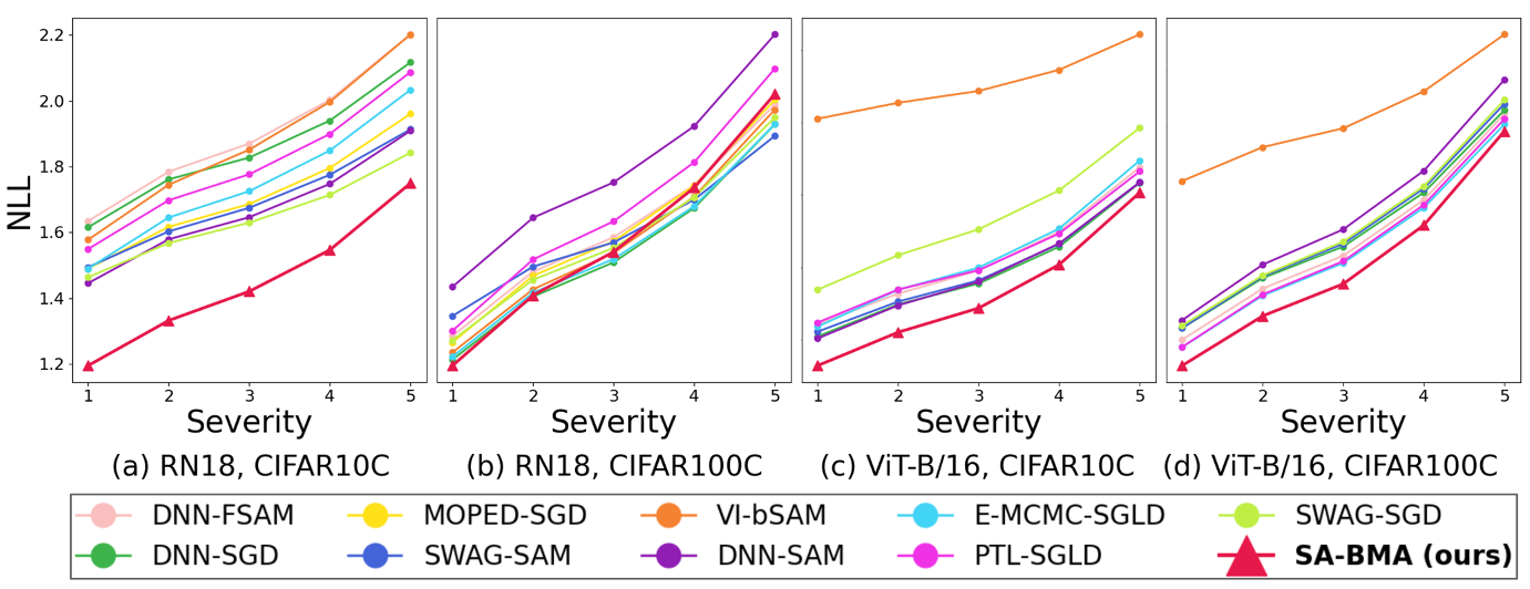
Figure 10: NLL performance of ResNet 18 and ViT-B/16 on corrupted CIFAR10 and CIFAR100, respectively [75].

We provide the detailed results of three repeated experiments with corrupted sets.

(a) RN18 CIFAR10C

Method Optim Severity 1 2 3 4 5 ACC $\uparrow$ NLL $\downarrow$ ACC $\uparrow$ NLL $\downarrow$ ACC $\uparrow$ NLL $\downarrow$ ACC $\uparrow$ NLL $\downarrow$ ACC $\uparrow$ NLL $\downarrow$ DNN SGD $49.57_{\pm{0.97}}$ $1.49_{\pm{0.02}}$ $45.78_{\pm{1.43}}$ $1.62_{\pm{0.04}}$ $43.78_{\pm{1.44}}$ $1.69_{\pm{0.04}}$ $40.83_{\pm{1.59}}$ $1.80_{\pm{0.06}}$ $36.30_{\pm{1.79}}$ $1.96_{\pm{0.08}}$ SAM $50.23_{\pm{2.11}}$ $1.62_{\pm{0.07}}$ $46.56_{\pm{2.00}}$ $1.76_{\pm{0.03}}$ $44.59_{\pm{2.26}}$ $1.83_{\pm{0.03}}$ $41.85_{\pm{2.42}}$ $1.94_{\pm{0.04}}$ $37.33_{\pm{2.52}}$ $2.12_{\pm{0.07}}$ FSAM $48.76_{\pm{4.00}}$ $1.63_{\pm{0.03}}$ $45.11_{\pm{3.91}}$ $1.78_{\pm{0.01}}$ $42.94_{\pm{3.88}}$ $1.87_{\pm{0.03}}$ $40.06_{\pm{3.85}}$ $2.00_{\pm{0.08}}$ 3$5.70_{\pm{3.50}}$ $2.20_{\pm{0.12}}$ SWAG SGD $50.05_{\pm{0.76}}$ $1.55_{\pm{0.09}}$ $46.31_{\pm{1.16}}$ $1.70_{\pm{0.11}}$ $44.17_{\pm{1.07}}$ $1.78_{\pm{0.11}}$ $41.20_{\pm{1.13}}$ $1.90_{\pm{0.13}}$ $36.64_{\pm{1.26}}$ $2.09_{\pm{0.15}}$ F-SWAG SAM $51.37_{\pm{1.08}}$ $1.49_{\pm{0.05}}$ $47.35_{\pm{0.71}}$ $1.64_{\pm{0.04}}$ $45.16_{\pm{0.66}}$ $1.72_{\pm{0.06}}$ $42.01_{\pm{0.57}}$ $1.85_{\pm{0.06}}$ $37.27_{\pm{0.64}}$ $2.03_{\pm{0.07}}$ VI bSAM $49.20_{\pm{2.40}}$ $1.46_{\pm{0.05}}$ $45.35_{\pm{1.93}}$ $1.57_{\pm{0.04}}$ $43.07_{\pm{2.10}}$ $1.63_{\pm{0.04}}$ $40.12_{\pm{1.74}}$ $1.71_{\pm{0.03}}$ $35.50_{\pm{1.36}}$ $1.84_{\pm{0.02}}$ MOPED SGD $50.72_{\pm{0.80}}$ $1.58_{\pm{0.11}}$ $46.87_{\pm{0.32}}$ $1.74_{\pm{0.11}}$ $44.52_{\pm{0.39}}$ $1.85_{\pm{0.12}}$ $41.38_{\pm{0.29}}$ $2.00_{\pm{0.12}}$ $36.73_{\pm{0.17}}$ $2.20_{\pm{0.10}}$ E-MCMC SGLD $49.86_{\pm{1.54}}$ $1.49_{\pm{0.03}}$ $46.17_{\pm{1.55}}$ $1.60_{\pm{0.04}}$ $44.07_{\pm{1.72}}$ $1.67_{\pm{0.07}}$ $41.05_{\pm{1.65}}$ $1.77_{\pm{0.10}}$ $36.53_{\pm{1.74}}$ $1.91_{\pm{0.13}}$ PTL SGLD $50.44_{\pm{1.65}}$ $1.45_{\pm{0.06}}$ $46.22_{\pm{1.96}}$ $1.58_{\pm{0.09}}$ $44.06_{\pm{1.67}}$ $1.65_{\pm{0.09}}$ $41.02_{\pm{1.66}}$ $1.75_{\pm{0.11}}$ $36.14_{\pm{1.51}}$ $1.91_{\pm{0.13}}$ SA-BMA (VI) $\textbf{58.53}_{\pm{0.75}}$ $\textbf{1.19}_{\pm{0.02}}$ $\textbf{53.72}_{\pm{0.70}}$ $\textbf{1.33}_{\pm{0.00}}$ $\textbf{50.61}_{\pm{0.84}}$ $\textbf{1.42}_{\pm{0.01}}$ $\textbf{46.76}_{\pm{1.15}}$ $\textbf{1.55}_{\pm{0.03}}$ $\textbf{40.70}_{\pm{1.34}}$ $\textbf{1.75}_{\pm{0.05}}$

(b) RN18 CIFAR100C

Method Optim Severity 1 2 3 4 5 ACC $\uparrow$ NLL $\downarrow$ ACC $\uparrow$ NLL $\downarrow$ ACC $\uparrow$ NLL $\downarrow$ ACC $\uparrow$ NLL $\downarrow$ ACC $\uparrow$ NLL $\downarrow$ DNN SGD $36.01_{\pm{0.86}}$ $2.55_{\pm{0.06}}$ $31.81_{\pm{0.73}}$ $2.79_{\pm{0.06}}$ $29.75_{\pm{0.57}}$ $2.91_{\pm{0.04}}$ $26.73_{\pm{0.25}}$ $3.11_{\pm{0.02}}$ $22.20_{\pm{0.08}}$ $3.40_{\pm{0.00}}$ SAM $37.94_{\pm{0.52}}$ $2.46_{\pm{0.02}}$ $33.57_{\pm{0.50}}$ $\textbf{2.69}_{\pm{0.03}}$ $31.46_{\pm{0.67}}$ $\textbf{2.82}_{\pm{0.03}}$ $28.19_{\pm{0.75}}$ $3.02_{\pm{0.05}}$ $23.32_{\pm{0.69}}$ $3.33_{\pm{0.06}}$ FSAM $36.46_{\pm{0.44}}$ $2.53_{\pm{0.05}}$ $32.24_{\pm{0.36}}$ $2.77_{\pm{0.04}}$ $30.19_{\pm{0.42}}$ $2.90_{\pm{0.03}}$ $27.12_{\pm{0.37}}$ $3.10_{\pm{0.02}}$ $22.48_{\pm{0.39}}$ $3.42_{\pm{0.01}}$ SWAG SGD $35.84_{\pm{5.17}}$ $2.62_{\pm{0.30}}$ $32.43_{\pm{4.55}}$ $2.81_{\pm{0.27}}$ $30.71_{\pm{4.21}}$ $2.89_{\pm{0.25}}$ $28.13_{\pm{3.81}}$ $3.05_{\pm{0.22}}$ $24.24_{\pm{2.99}}$ $\textbf{3.29}_{\pm{0.17}}$ F-SWAG SAM $37.10_{\pm{0.60}}$ $2.49_{\pm{0.03}}$ $32.84_{\pm{0.62}}$ $2.72_{\pm{0.03}}$ $30.59_{\pm{0.72}}$ $2.86_{\pm{0.04}}$ $27.43_{\pm{0.91}}$ $3.06_{\pm{0.06}}$ $22.74_{\pm{0.93}}$ $3.38_{\pm{0.08}}$ VI bSAM $36.20_{\pm{0.59}}$ $2.73_{\pm{0.03}}$ $32.48_{\pm{0.34}}$ $2.99_{\pm{0.03}}$ $30.66_{\pm{0.33}}$ $3.12_{\pm{0.02}}$ $27.94_{\pm{0.14}}$ $3.32_{\pm{0.05}}$ $23.66_{\pm{0.29}}$ $3.66_{\pm{0.06}}$ MOPED SGD $38.20_{\pm{0.57}}$ $2.47_{\pm{0.02}}$ $33.77_{\pm{0.59}}$ $2.71_{\pm{0.03}}$ $31.70_{\pm{0.75}}$ $2.83_{\pm{0.03}}$ $28.56_{\pm{0.77}}$ $\textbf{3.03}_{\pm{0.04}}$ $23.72_{\pm{0.78}}$ $3.33_{\pm{0.05}}$ E-MCMC SGLD $36.49_{\pm{0.89}}$ $2.57_{\pm{0.06}}$ $32.25_{\pm{0.76}}$ $2.83_{\pm{0.06}}$ $30.22_{\pm{0.63}}$ $2.97_{\pm{0.05}}$ $27.17_{\pm{0.38}}$ $3.19_{\pm{0.03}}$ $22.54_{\pm{0.27}}$ $3.54_{\pm{0.01}}$ PTL SGLD $36.43_{\pm{0.35}}$ $2.53_{\pm{0.03}}$ $32.24_{\pm{0.40}}$ $2.76_{\pm{0.03}}$ $30.20_{\pm{0.42}}$ $2.87_{\pm{0.03}}$ $27.17_{\pm{0.55}}$ $3.06_{\pm{0.04}}$ $22.56_{\pm{0.54}}$ $3.36_{\pm{0.05}}$ SA-BMA (VI) $\textbf{39.41}_{\pm{0.72}}$ $\textbf{2.44}_{\pm{0.04}}$ $\textbf{35.07}_{\pm{0.64}}$ $2.70_{\pm{0.05}}$ $\textbf{32.75}_{\pm{0.71}}$ $2.86_{\pm{0.05}}$ $\textbf{29.41}_{\pm{0.67}}$ $3.10_{\pm{0.05}}$ $\textbf{24.25}_{\pm{0.70}}$ $3.44_{\pm{0.05}}$

(c) VIT-B/16 CIFAR10C

Method Optim Severity 1 2 3 4 5 ACC $\uparrow$ NLL $\downarrow$ ACC $\uparrow$ NLL $\downarrow$ ACC $\uparrow$ NLL $\downarrow$ ACC $\uparrow$ NLL $\downarrow$ ACC $\uparrow$ NLL $\downarrow$ DNN SGD $79.62_{\pm 0.56}$ $0.64_{\pm 0.06}$ $76.47_{\pm 0.67}$ $0.73_{\pm 0.06}$ $74.10_{\pm 0.83}$ $0.79_{\pm 0.05}$ $70.42_{\pm 1.23}$ $0.90_{\pm 0.05}$ $64.41_{\pm{1.85}}$ $1.08_{\pm{0.05}}$ SAM $79.78_{\pm 0.49}$ $0.61_{\pm 0.01}$ $76.59_{\pm 0.64}$ $0.70_{\pm 0.02}$ $74.58_{\pm 0.94}$ $0.75_{\pm 0.02}$ $71.12_{\pm 1.06}$ $0.86_{\pm 0.03}$ $65.26_{\pm 1.46}$ $1.03_{\pm 0.04}$ FSAM $79.87_{\pm 0.83}$ $0.62_{\pm 0.02}$ $76.78_{\pm 0.78}$ $0.70_{\pm 0.02}$ $74.70_{\pm 0.60}$ $0.76_{\pm 0.01}$ $71.29_{\pm 0.49}$ $0.86_{\pm 0.01}$ $65.53_{\pm 0.56}$ $1.03_{\pm 0.03}$ SWAG SGD $76.58_{\pm 1.69}$ $1.21_{\pm 0.04}$ $73.45_{\pm 1.98}$ $1.25_{\pm 0.04}$ $71.20_{\pm 2.18}$ $1.29_{\pm 0.04}$ $67.54_{\pm 2.46}$ $1.35_{\pm 0.04}$ $61.65_{\pm 2.82}$ $1.44_{\pm 0.04}$ F-SWAG SAM $81.03_{\pm 2.20}$ $0.60_{\pm 0.05}$ $77.73_{\pm 2.63}$ $0.69_{\pm 0.06}$ $75.45_{\pm 2.96}$ $0.76_{\pm 0.07}$ $71.82_{\pm 3.31}$ $0.87_{\pm 0.08}$ $66.05_{\pm 3.59}$ $1.03_{\pm 0.10}$ VI bSAM $78.80_{\pm 1.18}$ $0.64_{\pm 0.04}$ $75.43_{\pm 1.14}$ $0.74_{\pm 0.04}$ $73.45_{\pm 1.43}$ $0.80_{\pm 0.04}$ $70.07_{\pm 1.50}$ $0.91_{\pm 0.05}$ $64.21_{\pm 1.57}$ $1.09_{\pm 0.05}$ E-MCMC SGLD $78.91_{\pm 2.31}$ $0.65_{\pm 0.08}$ $75.78_{\pm 2.36}$ $0.74_{\pm 0.08}$ $73.94_{\pm 2.56}$ $0.79_{\pm 0.09}$ $70.66_{\pm 2.63}$ $0.89_{\pm 0.10}$ $65.07_{\pm 2.77}$ $1.06_{\pm 0.11}$ PTL SGLD $76.26_{\pm 2.46}$ $0.74_{\pm 0.06}$ $72.36_{\pm 2.41}$ $0.83_{\pm 0.06}$ $69.61_{\pm 2.46}$ $0.90_{\pm 0.07}$ $65.47_{\pm 2.52}$ $1.01_{\pm 0.07}$ $59.04_{\pm 2.26}$ $1.18_{\pm 0.06}$ SA-BMA (VI) $\textbf{82.89}_{\pm 1.09}$ $\textbf{0.53}_{\pm 0.04}$ $\textbf{79.68}_{\pm 1.26}$ $\textbf{0.62}_{\pm 0.04}$ $\textbf{77.30}_{\pm 1.43}$ $\textbf{0.69}_{\pm 0.05}$ $\textbf{73.41}_{\pm 1.62}$ $\textbf{0.81}_{\pm 0.06}$ $\textbf{66.94}_{\pm 1.79}$ $\textbf{1.01}_{\pm 0.07}$

(d) VIT-B/16 CIFAR100C

Method Optim Severity 1 2 3 4 5 ACC $\uparrow$ NLL $\downarrow$ ACC $\uparrow$ NLL $\downarrow$ ACC $\uparrow$ NLL $\downarrow$ ACC $\uparrow$ NLL $\downarrow$ ACC $\uparrow$ NLL $\downarrow$ DNN SGD $62.19_{\pm 0.52}$ $1.42_{\pm 0.02}$ $57.81_{\pm 0.37}$ $1.61_{\pm 0.02}$ $55.04_{\pm 0.14}$ $1.73_{\pm 0.02}$ $50.73_{\pm 0.24}$ $1.93_{\pm 0.01}$ $44.12_{\pm 0.39}$ $2.24_{\pm 0.01}$ SAM $61.90_{\pm 0.53}$ $1.47_{\pm 0.02}$ $57.49_{\pm 0.43}$ $1.65_{\pm 0.02}$ $54.80_{\pm 0.29}$ $1.76_{\pm 0.01}$ $50.52_{\pm 0.25}$ $1.96_{\pm 0.01}$ $44.04_{\pm 0.24}$ $2.26_{\pm 0.01}$ FSAM $61.70_{\pm 0.52}$ $1.47_{\pm 0.02}$ $57.16_{\pm 0.44}$ $1.65_{\pm 0.02}$ $54.46_{\pm 0.37}$ $1.77_{\pm 0.02}$ $50.11_{\pm 0.39}$ $1.97_{\pm 0.01}$ $43.53_{\pm 0.42}$ $2.28_{\pm 0.01}$ SWAG SGD $59.19_{\pm 0.90}$ $2.00_{\pm 0.03}$ $55.45_{\pm 0.88}$ $2.12_{\pm 0.03}$ $53.34_{\pm 0.94}$ $2.19_{\pm 0.03}$ $49.44_{\pm 0.81}$ $2.33_{\pm 0.03}$ $43.71_{\pm 0.93}$ $2.53_{\pm 0.03}$ F-SWAG SAM $59.55_{\pm 2.94}$ $1.49_{\pm 0.11}$ $55.10_{\pm 2.82}$ $1.70_{\pm 0.10}$ $52.37_{\pm 2.80}$ $1.82_{\pm 0.10}$ $48.18_{\pm 2.63}$ $2.04_{\pm 0.09}$ $41.84_{\pm 2.43}$ $2.37_{\pm 0.09}$ VI bSAM $62.36_{\pm 0.73}$ $1.40_{\pm 0.03}$ $57.97_{\pm 0.70}$ $1.58_{\pm 0.03}$ $55.32_{\pm 0.61}$ $1.70_{\pm 0.03}$ $51.09_{\pm 0.49}$ $1.90_{\pm 0.03}$ $44.77_{\pm 0.42}$ $2.21_{\pm 0.03}$ E-MCMC SGLD $62.28_{\pm 0.47}$ $1.40_{\pm 0.02}$ $57.84_{\pm 0.46}$ $1.59_{\pm 0.02}$ $55.14_{\pm 0.29}$ $1.71_{\pm 0.02}$ $50.87_{\pm 0.21}$ $1.91_{\pm 0.02}$ $44.49_{\pm 0.13}$ $2.22_{\pm 0.02}$ PTL SGLD $61.84_{\pm 0.33}$ $1.47_{\pm 0.02}$ $57.36_{\pm 0.22}$ $1.66_{\pm 0.02}$ $54.47_{\pm 0.08}$ $1.78_{\pm 0.01}$ $50.03_{\pm 0.23}$ $1.98_{\pm 0.01}$ $43.34_{\pm 0.36}$ $2.29_{\pm 0.01}$ SA-BMA (VI) $\textbf{63.91}_{\pm 0.02}$ $\textbf{1.33}_{\pm 0.00}$ $\textbf{59.70}_{\pm 0.00}$ $\textbf{1.51}_{\pm 0.00}$ $\textbf{57.00}_{\pm 0.01}$ $\textbf{1.63}_{\pm 0.00}$ $\textbf{52.51}_{\pm 0.03}$ $\textbf{1.84}_{\pm 0.00}$ $\textbf{45.39}_{\pm 0.04}$ $\textbf{2.18}_{\pm 0.00}$

Appendix F Additional Loss Surface Of Sampled Model

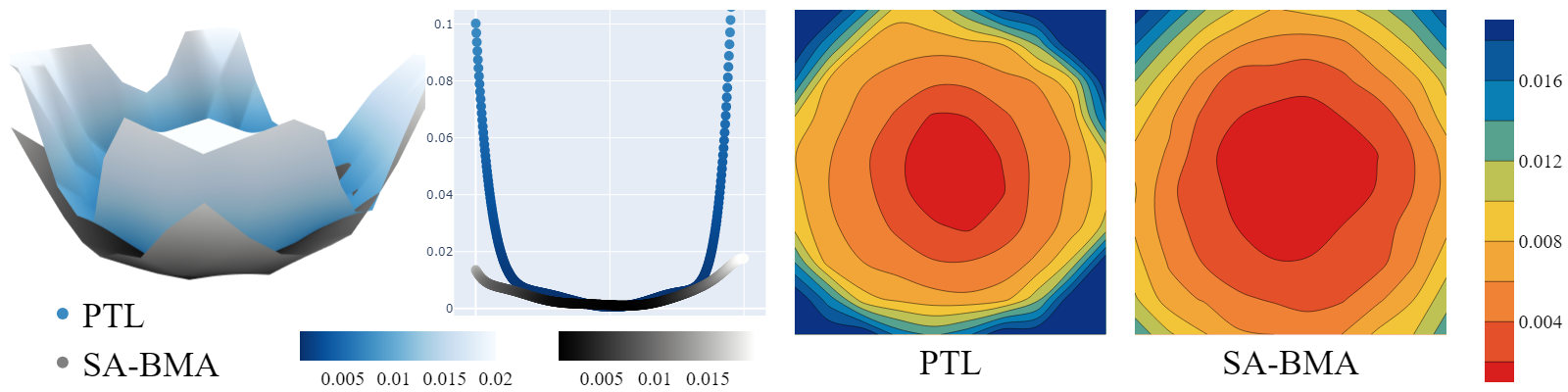
(a) seed 1

(b) seed 2

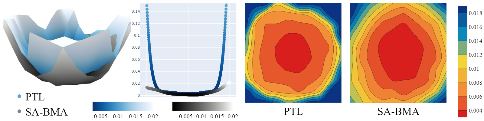
(c) seed 3

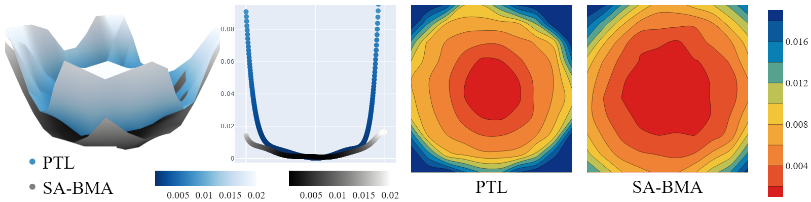
(d) seed 4

Figure 11: Four instances of sampled weights, including (b) as presented in Figure 4. Across all plots, it is consistently observed that SA-BMA converges to a flatter loss surface compared to PTL.

We adopt corrupted dataset CIFAR10/100C to test the robustness over distribution shift. The corrupted dataset transform the CIFAR10/100-test dataset, which has been modified to shift the distribution of the test data further away from the training data. It contains 19 kinds of corrupt options, such as varying brightness or contrast to adding Gaussian noise. The severity level indicates the strength of the transformation and is typically expressed as a number from 1 to 5, where the higher the number, the stronger the transformation.

As shown in Figure 4, we sampled four model parameters from the posterior, which were trained on CIFAR10 with RN18. It shows the consistent and robust trend of flatness of SA-BMA in the loss surface. In Figure 11, commencing with the leftmost panel, a 3D surface plot illustrates the loss surface, revealing the SA-BMA model’s comparatively flatter topology against the PTL model. This initial plot intuitively demonstrates that the SA-BMA model exhibits a flatter loss surface compared to the PTL model. Following this, the second visualization compresses the information along a diagonal plane into a 1D scatter plot. This transformation reveals areas obscured in the 3D view, highlighting that SA-BMA maintains a considerably flatter and lower-loss landscape. The third and fourth images showcase the loss surface through 2D contour plots, from which one can easily discern that the area representing the lowest loss is significantly more expansive for SA-BMA than for PTL.

Appendix G Limitation and Future Works

This study has several limitations. Firstly, calculating the FIM in weight space rather than output space makes it intractable to compute the FIM for the entire model parameter. Obtaining the FIM for the entire model weight space could lead to much more powerful performance improvements, making it one potential direction for future work. Secondly, the assumption of the existence of pre-trained models is necessary. In situations where pre-trained weights are not available, performance improvements may be somewhat limited. When training from scratch, additional research utilizing the concepts of this paper to converge the model to flat minima is also possible.

References

- Devlin et al. [2018] Jacob Devlin, Ming-Wei Chang, Kenton Lee, and Kristina Toutanova. Bert: Pre-training of deep bidirectional transformers for language understanding. arXiv preprint arXiv:1810.04805, 2018.
- Hendrycks et al. [2019] Dan Hendrycks, Kimin Lee, and Mantas Mazeika. Using pre-training can improve model robustness and uncertainty. In International conference on machine learning, pages 2712–2721. PMLR, 2019.
- Jiang et al. [2019] Haoming Jiang, Pengcheng He, Weizhu Chen, Xiaodong Liu, Jianfeng Gao, and Tuo Zhao. Smart: Robust and efficient fine-tuning for pre-trained natural language models through principled regularized optimization. arXiv preprint arXiv:1911.03437, 2019.
- Wortsman et al. [2022] Mitchell Wortsman, Gabriel Ilharco, Jong Wook Kim, Mike Li, Simon Kornblith, Rebecca Roelofs, Raphael Gontijo Lopes, Hannaneh Hajishirzi, Ali Farhadi, Hongseok Namkoong, et al. Robust fine-tuning of zero-shot models. In Proceedings of the IEEE/CVF Conference on Computer Vision and Pattern Recognition, pages 7959–7971, 2022.
- Choi et al. [2024] Caroline Choi, Yoonho Lee, Annie Chen, Allan Zhou, Aditi Raghunathan, and Chelsea Finn. Autoft: Robust fine-tuning by optimizing hyperparameters on ood data. arXiv preprint arXiv:2401.10220, 2024.
- MacKay [1992a] David JC MacKay. A practical bayesian framework for backpropagation networks. Neural computation, 4(3):448–472, 1992a.
- Hinton and Van Camp [1993] Geoffrey E Hinton and Drew Van Camp. Keeping the neural networks simple by minimizing the description length of the weights. In Proceedings of the sixth annual conference on Computational learning theory, pages 5–13, 1993.
- Neal [2012] Radford M Neal. Bayesian learning for neural networks, volume 118. Springer Science & Business Media, 2012.
- Wasserman [2000] Larry Wasserman. Bayesian model selection and model averaging. Journal of mathematical psychology, 44(1):92–107, 2000.
- Fragoso et al. [2018] Tiago M Fragoso, Wesley Bertoli, and Francisco Louzada. Bayesian model averaging: A systematic review and conceptual classification. International Statistical Review, 86(1):1–28, 2018.
- Wilson and Izmailov [2020] Andrew G Wilson and Pavel Izmailov. Bayesian deep learning and a probabilistic perspective of generalization. Advances in neural information processing systems, 33:4697–4708, 2020.
- Zeng and Van den Broeck [2024] Zhe Zeng and Guy Van den Broeck. Collapsed inference for bayesian deep learning. Advances in Neural Information Processing Systems, 36, 2024.
- Kapoor et al. [2022] Sanyam Kapoor, Wesley J Maddox, Pavel Izmailov, and Andrew G Wilson. On uncertainty, tempering, and data augmentation in bayesian classification. Advances in Neural Information Processing Systems, 35:18211–18225, 2022.
- Kristiadi et al. [2022a] Agustinus Kristiadi, Matthias Hein, and Philipp Hennig. Being a bit frequentist improves bayesian neural networks. In International Conference on Artificial Intelligence and Statistics, pages 529–545. PMLR, 2022a.
- Shwartz-Ziv et al. [2022] Ravid Shwartz-Ziv, Micah Goldblum, Hossein Souri, Sanyam Kapoor, Chen Zhu, Yann LeCun, and Andrew Gordon Wilson. Pre-train your loss: Easy bayesian transfer learning with informative priors. arXiv preprint arXiv:2205.10279, 2022.
- Zhuang et al. [2020] Fuzhen Zhuang, Zhiyuan Qi, Keyu Duan, Dongbo Xi, Yongchun Zhu, Hengshu Zhu, Hui Xiong, and Qing He. A comprehensive survey on transfer learning. Proceedings of the IEEE, 109(1):43–76, 2020.
- Izmailov et al. [2021] Pavel Izmailov, Sharad Vikram, Matthew D Hoffman, and Andrew Gordon Gordon Wilson. What are bayesian neural network posteriors really like? In International conference on machine learning, pages 4629–4640. PMLR, 2021.
- Kristiadi et al. [2022b] Agustinus Kristiadi, Runa Eschenhagen, and Philipp Hennig. Posterior refinement improves sample efficiency in bayesian neural networks. Advances in Neural Information Processing Systems, 35:30333–30346, 2022b.
- Hochreiter and Schmidhuber [1997] Sepp Hochreiter and Jürgen Schmidhuber. Flat minima. Neural computation, 9(1):1–42, 1997.
- Keskar et al. [2016] Nitish Shirish Keskar, Dheevatsa Mudigere, Jorge Nocedal, Mikhail Smelyanskiy, and Ping Tak Peter Tang. On large-batch training for deep learning: Generalization gap and sharp minima. arXiv preprint arXiv:1609.04836, 2016.
- Neyshabur et al. [2017] Behnam Neyshabur, Srinadh Bhojanapalli, David McAllester, and Nati Srebro. Exploring generalization in deep learning. Advances in neural information processing systems, 30, 2017.
- MacKay [2003] David JC MacKay. Information theory, inference and learning algorithms. Cambridge university press, 2003.
- Zhang et al. [2018] Guodong Zhang, Shengyang Sun, David Duvenaud, and Roger Grosse. Noisy natural gradient as variational inference. In International conference on machine learning, pages 5852–5861. PMLR, 2018.
- Li and Zhang [2023] Bolian Li and Ruqi Zhang. Entropy-mcmc: Sampling from flat basins with ease. In NeurIPS 2023 Workshop on Symmetry and Geometry in Neural Representations, 2023.
- Möllenhoff and Khan [2022] Thomas Möllenhoff and Mohammad Emtiyaz Khan. Sam as an optimal relaxation of bayes. arXiv preprint arXiv:2210.01620, 2022.
- Welling and Teh [2011] Max Welling and Yee W Teh. Bayesian learning via stochastic gradient langevin dynamics. In Proceedings of the 28th international conference on machine learning (ICML-11), pages 681–688, 2011.
- Chen et al. [2014] Tianqi Chen, Emily Fox, and Carlos Guestrin. Stochastic gradient hamiltonian monte carlo. In International conference on machine learning, pages 1683–1691. PMLR, 2014.
- Graves [2011] Alex Graves. Practical variational inference for neural networks. Advances in neural information processing systems, 24, 2011.
- Ranganath et al. [2014] Rajesh Ranganath, Sean Gerrish, and David Blei. Black box variational inference. In Artificial intelligence and statistics, pages 814–822. PMLR, 2014.
- Blundell et al. [2015] Charles Blundell, Julien Cornebise, Koray Kavukcuoglu, and Daan Wierstra. Weight uncertainty in neural network. In International conference on machine learning, pages 1613–1622. PMLR, 2015.
- MacKay [1992b] David JC MacKay. Bayesian interpolation. Neural computation, 4(3):415–447, 1992b.
- Ritter et al. [2018] Hippolyt Ritter, Aleksandar Botev, and David Barber. A scalable laplace approximation for neural networks. In 6th International Conference on Learning Representations, ICLR 2018-Conference Track Proceedings, volume 6. International Conference on Representation Learning, 2018.
- Daxberger et al. [2021a] Erik Daxberger, Agustinus Kristiadi, Alexander Immer, Runa Eschenhagen, Matthias Bauer, and Philipp Hennig. Laplace redux-effortless bayesian deep learning. Advances in Neural Information Processing Systems, 34:20089–20103, 2021a.
- Gal and Ghahramani [2016] Yarin Gal and Zoubin Ghahramani. Dropout as a bayesian approximation: Representing model uncertainty in deep learning. In international conference on machine learning, pages 1050–1059. PMLR, 2016.
- Maddox et al. [2019] Wesley J Maddox, Pavel Izmailov, Timur Garipov, Dmitry P Vetrov, and Andrew Gordon Wilson. A simple baseline for bayesian uncertainty in deep learning. Advances in Neural Information Processing Systems, 32, 2019.
- Hochreiter and Schmidhuber [1994] Sepp Hochreiter and Jürgen Schmidhuber. Simplifying neural nets by discovering flat minima. Advances in neural information processing systems, 7, 1994.
- Foret et al. [2020] Pierre Foret, Ariel Kleiner, Hossein Mobahi, and Behnam Neyshabur. Sharpness-aware minimization for efficiently improving generalization. arXiv preprint arXiv:2010.01412, 2020.
- Jastrzebski et al. [2020] Stanislaw Jastrzebski, Maciej Szymczak, Stanislav Fort, Devansh Arpit, Jacek Tabor, Kyunghyun Cho, and Krzysztof Geras. The break-even point on optimization trajectories of deep neural networks. arXiv preprint arXiv:2002.09572, 2020.
- Baldassi et al. [2015] Carlo Baldassi, Alessandro Ingrosso, Carlo Lucibello, Luca Saglietti, and Riccardo Zecchina. Subdominant dense clusters allow for simple learning and high computational performance in neural networks with discrete synapses. Physical review letters, 115(12):128101, 2015.
- Baldassi et al. [2016] Carlo Baldassi, Christian Borgs, Jennifer T Chayes, Alessandro Ingrosso, Carlo Lucibello, Luca Saglietti, and Riccardo Zecchina. Unreasonable effectiveness of learning neural networks: From accessible states and robust ensembles to basic algorithmic schemes. Proceedings of the National Academy of Sciences, 113(48):E7655–E7662, 2016.
- Chaudhari et al. [2019] Pratik Chaudhari, Anna Choromanska, Stefano Soatto, Yann LeCun, Carlo Baldassi, Christian Borgs, Jennifer Chayes, Levent Sagun, and Riccardo Zecchina. Entropy-sgd: Biasing gradient descent into wide valleys. Journal of Statistical Mechanics: Theory and Experiment, 2019(12):124018, 2019.
- Dziugaite and Roy [2018] Gintare Karolina Dziugaite and Daniel Roy. Entropy-sgd optimizes the prior of a pac-bayes bound: Generalization properties of entropy-sgd and data-dependent priors. In International Conference on Machine Learning, pages 1377–1386. PMLR, 2018.
- Kim et al. [2022] Minyoung Kim, Da Li, Shell X Hu, and Timothy Hospedales. Fisher sam: Information geometry and sharpness aware minimisation. In International Conference on Machine Learning, pages 11148–11161. PMLR, 2022.
- Du et al. [2021] Jiawei Du, Hanshu Yan, Jiashi Feng, Joey Tianyi Zhou, Liangli Zhen, Rick Siow Mong Goh, and Vincent YF Tan. Efficient sharpness-aware minimization for improved training of neural networks. arXiv preprint arXiv:2110.03141, 2021.
- Du et al. [2022] Jiawei Du, Daquan Zhou, Jiashi Feng, Vincent YF Tan, and Joey Tianyi Zhou. Sharpness-aware training for free. arXiv preprint arXiv:2205.14083, 2022.
- Liu et al. [2022] Yong Liu, Siqi Mai, Xiangning Chen, Cho-Jui Hsieh, and Yang You. Towards efficient and scalable sharpness-aware minimization. In Proceedings of the IEEE/CVF Conference on Computer Vision and Pattern Recognition, pages 12360–12370, 2022.
- Mi et al. [2022] Peng Mi, Li Shen, Tianhe Ren, Yiyi Zhou, Xiaoshuai Sun, Rongrong Ji, and Dacheng Tao. Make sharpness-aware minimization stronger: A sparsified perturbation approach. Advances in Neural Information Processing Systems, 35:30950–30962, 2022.
- Mueller et al. [2024] Maximilian Mueller, Tiffany Vlaar, David Rolnick, and Matthias Hein. Normalization layers are all that sharpness-aware minimization needs. Advances in Neural Information Processing Systems, 36, 2024.
- Guo et al. [2017] Chuan Guo, Geoff Pleiss, Yu Sun, and Kilian Q Weinberger. On calibration of modern neural networks. In International conference on machine learning, pages 1321–1330. PMLR, 2017.
- He et al. [2016] Kaiming He, Xiangyu Zhang, Shaoqing Ren, and Jian Sun. Deep residual learning for image recognition. In Proceedings of the IEEE conference on computer vision and pattern recognition, pages 770–778, 2016.
- Ioffe and Szegedy [2015] Sergey Ioffe and Christian Szegedy. Batch normalization: Accelerating deep network training by reducing internal covariate shift. In International conference on machine learning, pages 448–456. pmlr, 2015.
- Weyl [1912] Hermann Weyl. Das asymptotische verteilungsgesetz der eigenwerte linearer partieller differentialgleichungen (mit einer anwendung auf die theorie der hohlraumstrahlung). Mathematische Annalen, 71(4):441–479, 1912.
- Izmailov et al. [2020] Pavel Izmailov, Wesley J Maddox, Polina Kirichenko, Timur Garipov, Dmitry Vetrov, and Andrew Gordon Wilson. Subspace inference for bayesian deep learning. In Uncertainty in Artificial Intelligence, pages 1169–1179. PMLR, 2020.
- Daxberger et al. [2021b] Erik Daxberger, Eric Nalisnick, James U Allingham, Javier Antorán, and José Miguel Hernández-Lobato. Bayesian deep learning via subnetwork inference. In International Conference on Machine Learning, pages 2510–2521. PMLR, 2021b.
- Sharma et al. [2023] Mrinank Sharma, Sebastian Farquhar, Eric Nalisnick, and Tom Rainforth. Do bayesian neural networks need to be fully stochastic? In International Conference on Artificial Intelligence and Statistics, pages 7694–7722. PMLR, 2023.
- Snoek et al. [2015] Jasper Snoek, Oren Rippel, Kevin Swersky, Ryan Kiros, Nadathur Satish, Narayanan Sundaram, Mostofa Patwary, Mr Prabhat, and Ryan Adams. Scalable bayesian optimization using deep neural networks. In International conference on machine learning, pages 2171–2180. PMLR, 2015.
- Daxberger et al. [2021c] Erik Daxberger, Agustinus Kristiadi, Alexander Immer, Runa Eschenhagen, Matthias Bauer, and Philipp Hennig. Laplace redux–effortless Bayesian deep learning. In NeurIPS, 2021c.
- Harrison et al. [2023] James Harrison, John Willes, and Jasper Snoek. Variational bayesian last layers. In Fifth Symposium on Advances in Approximate Bayesian Inference, 2023.
- Krizhevsky et al. [2009] Alex Krizhevsky, Geoffrey Hinton, et al. Learning multiple layers of features from tiny images. 2009.
- Nguyen et al. [2023] Van-Anh Nguyen, Tung-Long Vuong, Hoang Phan, Thanh-Toan Do, Dinh Phung, and Trung Le. Flat seeking bayesian neural networks. arXiv preprint arXiv:2302.02713, 2023.
- Krishnan et al. [2020] Ranganath Krishnan, Mahesh Subedar, and Omesh Tickoo. Specifying weight priors in bayesian deep neural networks with empirical bayes. In Proceedings of the AAAI Conference on Artificial Intelligence, volume 34, pages 4477–4484, 2020. URL https://ojs.aaai.org/index.php/AAAI/article/view/5875.
- Dosovitskiy et al. [2020] Alexey Dosovitskiy, Lucas Beyer, Alexander Kolesnikov, Dirk Weissenborn, Xiaohua Zhai, Thomas Unterthiner, Mostafa Dehghani, Matthias Minderer, Georg Heigold, Sylvain Gelly, et al. An image is worth 16x16 words: Transformers for image recognition at scale. arXiv preprint arXiv:2010.11929, 2020.
- Russakovsky et al. [2015] Olga Russakovsky, Jia Deng, Hao Su, Jonathan Krause, Sanjeev Satheesh, Sean Ma, Zhiheng Huang, Andrej Karpathy, Aditya Khosla, Michael Bernstein, et al. Imagenet large scale visual recognition challenge. International journal of computer vision, 115:211–252, 2015.
- Helber et al. [2019] Patrick Helber, Benjamin Bischke, Andreas Dengel, and Damian Borth. Eurosat: A novel dataset and deep learning benchmark for land use and land cover classification. IEEE Journal of Selected Topics in Applied Earth Observations and Remote Sensing, 12(7):2217–2226, 2019.
- Nilsback and Zisserman [2008] Maria-Elena Nilsback and Andrew Zisserman. Automated flower classification over a large number of classes. In 2008 Sixth Indian conference on computer vision, graphics & image processing, pages 722–729. IEEE, 2008.
- Parkhi et al. [2012] Omkar M Parkhi, Andrea Vedaldi, Andrew Zisserman, and CV Jawahar. Cats and dogs. In 2012 IEEE conference on computer vision and pattern recognition, pages 3498–3505. IEEE, 2012.
- Soomro et al. [2012] Khurram Soomro, Amir Roshan Zamir, and Mubarak Shah. Ucf101: A dataset of 101 human actions classes from videos in the wild. arXiv preprint arXiv:1212.0402, 2012.
- Recht et al. [2019] Benjamin Recht, Rebecca Roelofs, Ludwig Schmidt, and Vaishaal Shankar. Do imagenet classifiers generalize to imagenet? In International conference on machine learning, pages 5389–5400. PMLR, 2019.
- Hendrycks et al. [2021a] Dan Hendrycks, Steven Basart, Norman Mu, Saurav Kadavath, Frank Wang, Evan Dorundo, Rahul Desai, Tyler Zhu, Samyak Parajuli, Mike Guo, et al. The many faces of robustness: A critical analysis of out-of-distribution generalization. In Proceedings of the IEEE/CVF international conference on computer vision, pages 8340–8349, 2021a.
- Hendrycks et al. [2021b] Dan Hendrycks, Kevin Zhao, Steven Basart, Jacob Steinhardt, and Dawn Song. Natural adversarial examples. In Proceedings of the IEEE/CVF conference on computer vision and pattern recognition, pages 15262–15271, 2021b.
- Wang et al. [2019] Haohan Wang, Songwei Ge, Zachary Lipton, and Eric P Xing. Learning robust global representations by penalizing local predictive power. Advances in Neural Information Processing Systems, 32, 2019.
- Radford et al. [2021] Alec Radford, Jong Wook Kim, Chris Hallacy, Aditya Ramesh, Gabriel Goh, Sandhini Agarwal, Girish Sastry, Amanda Askell, Pamela Mishkin, Jack Clark, et al. Learning transferable visual models from natural language supervision. In International conference on machine learning, pages 8748–8763. PMLR, 2021.
- Zhu et al. [2023] Yao Zhu, Yuefeng Chen, Wei Wang, Xiaofeng Mao, Yue Wang, Zhigang Li, Jindong Wang, Xiangyang Ji, et al. Enhancing few-shot clip with semantic-aware fine-tuning. arXiv preprint arXiv:2311.04464, 2023.
- Lin et al. [2023] Zhiqiu Lin, Samuel Yu, Zhiyi Kuang, Deepak Pathak, and Deva Ramanan. Multimodality helps unimodality: Cross-modal few-shot learning with multimodal models. In Proceedings of the IEEE/CVF Conference on Computer Vision and Pattern Recognition, pages 19325–19337, 2023.
- Hendrycks and Dietterich [2019] Dan Hendrycks and Thomas Dietterich. Benchmarking neural network robustness to common corruptions and perturbations. arXiv preprint arXiv:1903.12261, 2019.
- Li et al. [2018] Hao Li, Zheng Xu, Gavin Taylor, Christoph Studer, and Tom Goldstein. Visualizing the loss landscape of neural nets. Advances in neural information processing systems, 31, 2018.
- Izmailov et al. [2018] Pavel Izmailov, Dmitrii Podoprikhin, Timur Garipov, Dmitry Vetrov, and Andrew Gordon Wilson. Averaging weights leads to wider optima and better generalization. arXiv preprint arXiv:1803.05407, 2018.
- Khan et al. [2018] Mohammad Khan, Didrik Nielsen, Voot Tangkaratt, Wu Lin, Yarin Gal, and Akash Srivastava. Fast and scalable bayesian deep learning by weight-perturbation in adam. In International conference on machine learning, pages 2611–2620. PMLR, 2018.
- Lee et al. [2024] Hyungi Lee, Giung Nam, Edwin Fong, and Juho Lee. Enhancing transfer learning with flexible nonparametric posterior sampling. arXiv preprint arXiv:2403.07282, 2024.
- Frankle et al. [2020] Jonathan Frankle, David J Schwab, and Ari S Morcos. Training batchnorm and only batchnorm: On the expressive power of random features in cnns. arXiv preprint arXiv:2003.00152, 2020.
- Gentle [2007] James E Gentle. Matrix algebra. Springer texts in statistics, Springer, New York, NY, doi, 10:978–0, 2007.
- Sidi [2017] Avram Sidi. Vector extrapolation methods with applications. SIAM, 2017.
- Wynn [1962] Peter Wynn. Acceleration techniques for iterated vector and matrix problems. Mathematics of Computation, 16(79):301–322, 1962.