Supporting Information for “Excitonic Bose-polarons in electron-hole bilayers”

I Sample

The sample used in this study is a coupled quantum well (CQW) heterostructure grown by molecular beam epitaxy. The CQW consists of two $15$-$\mathrm{nm}$-wide GaAs QWs separated by a $4$-$\mathrm{nm}$-thick Al_0.33Ga_0.67As barrier. An $n^{+}$ GaAs layer with $n_{\mathrm{Si}}\sim 10^{18}\,\mathrm{cm}^{-3}$ serves as a uniform bottom gate. The CQW is positioned $100\,\mathrm{nm}$ above the $n^{+}$ GaAs layer within the undoped $1$-$\mu\mathrm{m}$-thick Al_0.33Ga_0.67As layer. The CQW is located much closer to the bottom gate to minimize the effect of fringing electric fields in excitonic devices with patterned top gates [1]. The top semi-transparent gate is fabricated by applying $2\,\mathrm{nm}$ of Ti and $7\,\mathrm{nm}$ of Pt on a $7.5\,\mathrm{nm}$-thick GaAs cap layer. Applied gate voltage $V_{\mathrm{g}}=-2.5\,\mathrm{V}$ creates an electric field in the direction normal to the quantum wells. The corresponding band diagram of the CQW is shown in Fig. 1a of the main text. The applied voltage drives optically generated electrons (e) and holes (h) to the opposite quantum wells. This process is fast, so that the densities of minority particles (e’s in the h-layer and h’s in the e-layer) are orders of magnitude smaller than the densities of majority particles (e’s in the e-layer and h’s in the h-layer).

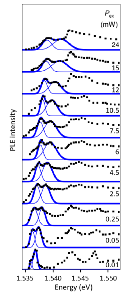
Figure S1: Gaussian fits to the ABP and RBP peaks in the measured PLE spectra (points, same as Fig. 2a of the main text). The individual fits are shown by the thin lines and their sum by the thick line. The peak energies found from the fits are presented in Fig. 2b of the main text.

II Optical measurements details

The PLE spectra (Fig. S1) probe spatially direct optical absorption within each QW. A spatially indirect absorption is much weaker and is not observed in PLE. The PL and PLE were measured $\sim 50\,\mu\mathrm{m}$ away from the laser excitation spot and $\sim 300\,\mathrm{ns}$ after the excitation pulse, where a cold and dense e-h system of temperature close to the lattice temperature was formed [2]. To facilitate comparison with prior PL measurements [2], we use similar optical excitation and detection protocol, as follows. The e-h system is generated by a Ti: Sapphire laser. An acousto-optic modulator is used for making laser pulses ($800\,\mathrm{ns}$ on, $400\,\mathrm{ns}$ off). A laser excitation spot with a mesa-shaped intensity profile and diameter $\sim 100\,\mu\mathrm{m}$ is created using an axicon. The signal is detected within a $50\,\mathrm{ns}$ window, which is much shorter than the IX lifetime, so that the signal variation during the measurement remains negligible [2]. The exciton density in the detection region is close to the density in the excitation spot because the separation is shorter than the IX propagation length and the time delay is shorter than the IX lifetime [2]. The IX PL spectra are measured using a spectrometer with resolution $0.2\,\mathrm{meV}$ and a liquid-nitrogen-cooled CCD coupled to a PicoStar HR TauTec time-gated intensifier. The experiments are performed in a variable-temperature ⁴He cryostat.

III PLE spectra

We used Gaussian fits for rough estimates of the ABP and RBP peak energies (Fig. S1). The actual ABP and RBP PLE lineshapes are complicated. In particular, their low-energy sides appearing near $1.536\,\mathrm{eV}$ have a non-Gaussian shoulder-like form (Fig. S1). The analysis of the lh-ABP and lh-RBP lines is also challenging because they appear on a background of optical transitions between free heavy holes and electrons, see the main text. Nevertheless, the variation of all the observed polaron energies with density are sufficiently strong and systematic (Fig. 2 of the main text). We note that the fit accuracy is lower for the highest $P_{\rm ex}$, in particular, due to the RBP peak broadening.

With increasing temperature, the ABP and RBP lines vanish and the PLE spectrum becomes step-like, reflecting the functional form of the e-h joint density of states in 2D (Fig. S2). At high temperatures, the absorption edge in the dense e-h system decreases compared to the low-temperature data (Fig. S2), as discussed in the main text.

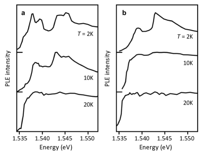
Figure S2: PLE spectra at $P_{\rm ex}=7.5$ (a) and 24 (b) mW at $T=2$, 10, and 20 K. At high temperatures, the excitonic peaks vanish and the PLE spectrum becomes step-like as 2D density of states.

IV Exciton binding energies

Few-body e-h bound states that can form in the CQW are listed in Table S I, together with their calculated binding energies. They include indirect excitons (IXs), direct excitons (DXs), and DX-IX biexcitons. The details of the calculations are presented below.

Complex	QW 1	QW 2	h $=$ hh	h $=$ lh
IX	e	hh	$2.99$
DX	e-h		$8.24$	$9.44$
DX-IX	e-h-e	hh	$0.96$	$1.26$
DX-IX	e	h-e-hh	$0.88$	$0.73$

Table S I: Calculated binding energies of various e-h complexes, in units of $\mathrm{meV}$, for zero gate voltage $V_{\mathrm{g}}=0$; ’hh’ and ’lh’ stand for the heavy hole and light hole, respectively.

The first step of the calculation is to solve for the single-particle states of the QWs. The electron states were determined from the Hamiltonian

$$H_{\mathrm{e}}=\frac{1}{2m_{\mathrm{e}}}{\mathbf{P}}^{2}+U_{\mathrm{e}}(z)\,,$$ (S1)

where $z$ is the coordinate perpendicular to the QW plane, ${\mathbf{P}}=(\mathbf{p},-i\hbar\partial_{z})$ is the momentum operator, $\mathbf{p}=\hbar\mathbf{k}_{\bot}$ is the in-plane momentum, and $m_{\mathrm{e}}=0.0665m_{0}$ is the effective electron mass in GaAs. The hole states were determined from the Hamiltonian [3, 4]

$$\begin{split}H_{\mathrm{h}}&=-\frac{1}{2m_{0}}\sum_{ij}P_{i}D_{ij}P_{j}+U_{\mathrm{h}}(z),\\ \hat{D}_{ij}&=\left(\frac{1}{2}\gamma_{1}+\frac{5}{4}\gamma_{2}\right)\delta_{ij}-\gamma_{2}{J_{i}}{J_{j}},\end{split}$$ (S2)

where $\gamma_{1}$ and $\gamma_{2}$ are the Luttinger parameters, $m_{0}$ is the free electron mass, and ${\mathbf{J}}=(J_{x},J_{y},J_{z})$ is the spin-$3/2$ angular momentum operator. The confining potentials $U_{\mathrm{e}}(z)$ and $U_{\mathrm{h}}(z)$ were chosen in the form

$$U_{\mathrm{e,h}}(z)=\begin{cases}0&\text{inside QW},\\ \mathcal{U}_{\mathrm{e,h}}&\text{outside QW}.\end{cases}$$ (S3)

For all the parameter values in our calculations we used those given in Ref. 5. We numerically diagonalized the Hamiltonians in Eqs. (S1) and (S2) and obtained the energy levels and wavefunctions $\varphi_{i}(z)$ where $i=\mathrm{e(h)}n$ for e(h) states of QW $n=1,2$. The energy-momentum dispersions of the first three hole subbands are plotted in Fig. S3. To facilitate comparison with published results [3, 4] (that appears to be good) the momentum on the horizontal axis is expressed in units of $\pi\times 10^{6}\,\mathrm{cm}^{-1}$.

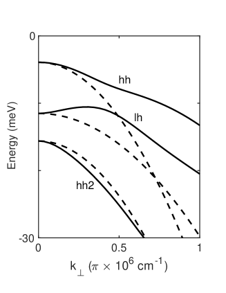
Figure S3: In-plane dispersion $\varepsilon_{\mathrm{h}}(\mathbf{k}_{\bot})$ for the first three hole subbands in units of $\mathrm{meV}$. The dashed lines are the dispersions obtained by neglecting the coupling between heavy and light holes (the off-diagonal terms of $H_{h}$).

Next, to define the effective mass $m_{\mathrm{h}}$ of the heavy hole (hh), we fitted its dispersion to a parabola over a range of momenta $0<k_{\bot}<a_{\mathrm{X}}^{-1}$, where $a_{\mathrm{X}}=(\kappa\hbar^{2}/e^{2})(m_{\mathrm{e}}^{-1}+m_{\mathrm{h}}^{-1})$ is again the exciton Bohr radius. We found $m_{\mathrm{h}}=0.217m_{0}=3.26m_{\mathrm{e}}$, so that $a_{\mathrm{X}}=12.7\,\mathrm{nm}$. Note that $a_{\mathrm{X}}^{-1}$ is about $0.25$ in the momentum units used in Fig. S3. The light hole (lh) dispersion is non-monotonic. For simplicity, we decided to neglect this dispersion altogether, i.e., to treat the lh mass as infinite.

To compute the binding energies of interest we approximated the momentum-space Coulomb interaction potential between particles of charge $e_{i}$ and $e_{j}$ by

$$\widetilde{V}_{ij}(\mathbf{k}_{\bot})=\frac{2\pi e_{i}e_{j}}{\kappa{k}_{\bot}}\int dzdz^{\prime}|\varphi_{i}(z)|^{2}\,|\varphi_{j}(z^{\prime})|^{2}\,e^{-{k}_{\bot}|z-z^{\prime}|}\,,$$ (S4)

which we further simplified as follows. For particles in the same layer, we used [4]

$$\widetilde{V}_{ij}(\mathbf{k}_{\bot})=\frac{2\pi e_{i}e_{j}}{\kappa{k}_{\bot}}\,\frac{1}{1+{k}_{\bot}\rho_{ij}}\,,$$ (S5a)

$$V_{ij}(\mathbf{r})=\frac{\pi}{2\rho_{ij}}\,\frac{e_{i}e_{j}}{\kappa}\,\left[\mathbf{H}_{0}\left(\frac{r}{\rho_{ij}}\right)-Y_{0}\left(\frac{r}{\rho_{ij}}\right)\right],$$ (S5b)

where the effective well widths $\rho_{\mathrm{e}n,\mathrm{e}n}=4.5\,\mathrm{nm}$, $\rho_{\mathrm{h}n,\mathrm{h}n}=3.81\,\mathrm{nm}$, and $\rho_{\mathrm{e}n,\mathrm{h}n}=4.17\,\mathrm{nm}$ (all for hh), were determined by numerically evaluating the integrals in Eq. (S4) and fitting the result to Eq. (S5a) at $0<{k}_{\bot}<a_{\mathrm{X}}^{-1}$. Equation (S5b) is known as the Rytova-Keldysh potential. This function approaches the Coulomb potential $e_{i}e_{j}/\kappa r$ at $r\gg\rho_{ij}$ and diverges logarithmically $(e_{i}e_{j}/\kappa\rho_{ij})\ln(\rho_{ij}/r)$ at $r\ll\rho_{ij}$; $\mathbf{H}_{0}(z)$ and $Y_{0}(z)$ are the Struve and Neumann functions, respectively.

For particles in opposite layers, we used $\rho_{ij}=0$, i.e., the Coulomb law:

$$\widetilde{V}_{ij}(\mathbf{k}_{\bot})=2\pi\frac{e_{i}e_{j}}{\kappa{k}_{\bot}}\,e^{-{k}_{\bot}d},$$ (S6a)

$$V_{ij}(\mathbf{r})=\frac{e_{i}e_{j}}{\kappa}\,\frac{1}{\sqrt{r^{2}+d^{2}}}\,,$$ (S6b)

where $d=19\,\mathrm{nm}$ is the center-to-center layer distance. These interlayer and intralayer potentials are plotted in Fig. S4. We neglected intersubband mixing because the energy separation between the subbands is relatively large, $5$–$7\,\mathrm{meV}$, see Fig. S3.

We computed the DX and IX binding energies $E_{\mathrm{X}}$ and ground-state wavefunctions $\phi_{\mathrm{X}}(\mathbf{k}_{\bot})$ by numerically solving the Wannier equation,

$$[\varepsilon_{\mathrm{e}}(\mathbf{k}_{\bot})+\varepsilon_{\mathrm{h}}(\mathbf{k}_{\bot})]\phi_{\mathrm{X}}(\mathbf{k}_{\bot}) +\Omega^{-1}\sum_{\mathbf{k}^{\prime}_{\bot}}\widetilde{V}_{\mathrm{e}k,\mathrm{h}n}(\mathbf{k}_{\bot}-\mathbf{k}^{\prime}_{\bot})\phi_{\mathrm{X}}(\mathbf{k}^{\prime}_{\bot})$$

$$=-E_{\mathrm{X}}\phi_{\mathrm{X}}(\mathbf{k}_{\bot})$$ (S7)

following Ref. 6. Here $\mathrm{X}\in\{\mathrm{DX},\mathrm{IX}\}$ is the exciton type, $\varepsilon_{\mathrm{e,h}}(\mathbf{k}_{\bot})=\hbar^{2}\mathbf{k}^{2}_{\bot}/2m_{\mathrm{e,h}}$ are the e(h) dispersions, and $\Omega$ is the area of the system.

Finally, we calculated the biexciton binding energies using the stochastic variational method (SVM), a highly accurate numerical technique for solving few-body quantum mechanics problems [7]. To this end we adopted the SVM code previously developed [8] for zero-thickness 2D layers ($\rho_{ij}\equiv 0$) and modified it to work with the interaction potential of Eq. (S5). We also used the SVM solver to verify the exciton binding energies $E_{\mathrm{X}}$ computed by the diagonalization method and found them to be in excellent agreement. Table S I summarizes the results for all the binding energies we calculated.

V Exciton-exciton interaction

V.1 IX-IX interaction

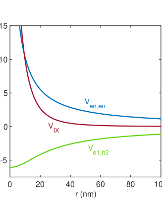
Figure S4: Model interaction potentials: intralayer potential $V_{\mathrm{e}n,\mathrm{e}n}=V_{\mathrm{h}n,\mathrm{h}n}$ [Eq. (S5b)], interlayer potential $V_{\mathrm{e}1,\mathrm{h}2}$ [Eq. (S6b)], and the IX-IX potential $V_{\mathrm{IX}}$ [Eq. (S11)].

Theoretical investigations of Bose polarons have been stimulated primarily by experiments with cold atoms. Transferring these methods to excitons must be done with caution because of important differences between two classes of systems. Atoms reach quantum degeneracy at very low temperatures in the n$\mathrm{K}$ or $\mu\mathrm{K}$-range. Since IXs have much smaller mass, their degeneracy temperature $T_{\mathrm{deg}}=2\pi T_{0}$ with $T_{0}\equiv\hbar^{2}n/m$ [9] is many orders of magnitude higher, e.g., $T_{\mathrm{deg}}=20\,\mathrm{K}$ for $m=m_{\mathrm{e}}+m_{\mathrm{h}}=0.285m_{0}$ and $n=10^{11}\,\mathrm{cm}^{-2}$.

Atoms typically form dilute, weakly nonideal BECs (Bose-Einstein condensates) for which the details of the interatomic interaction potential are unimportant. Instead, the interactions are parametrized by the $s$-wave scattering amplitude, which is proportional to the on-shell two-body $T$-matrix. In 2D, this $T$-matrix has a universal low-energy form

$$T(E)\simeq\frac{4\pi\hbar^{2}}{m}\left[\ln\left(-\frac{\hbar^{2}}{ma^{2}}\,\frac{1}{E}\right)\right]^{-1},\quad E\to 0,$$ (S8)

where $a$ is referred to as the scattering length. The $T$-matrix enters in equations for many key quantities of the system. For example, the chemical potential $\zeta$ of the BEC is given by

$$\zeta=Tn$$ (S9)

to the leading order in $na^{2}\ll 1$. In this equation, $T$ needs to be evaluated at energy $E\sim-\zeta$ [10, 11], so that Eq. (S9) is a self-consistent equation for $\zeta$ as a function of $n$. The solution can be presented in the form

$$\tilde{g}\equiv\frac{\zeta}{T_{\mathrm{0}}}=\frac{m}{\hbar^{2}}\,\frac{\zeta}{n}\simeq\frac{4\pi}{\ln\left({1}/{na^{2}}\right)}\,.$$ (S10)

The dimensionless parameter $\tilde{g}$ is a measure of BEC nonideality. For example, it determines the interaction-induced condensate depletion via $\tilde{g}/(2\pi)$ [11]. These formulas apply if $\tilde{g}\lesssim 1$ [12, 13], which translates to the condition on the boson density $na^{2}\lesssim 10^{-6}$. Despite the small numerical factor on the right-hand side of this inequality, it is not uncommon to have it fulfilled for cold atoms. In contrast, such densities are unrealistically low for IXs in GaAs heterostructures. As a result, scattering length $a$ is not useful for describing these excitonic systems. Their properties crucially depend on details of the IX-IX interaction and they are typically strongly coupled, $\tilde{g}\gg 1$.

One common model for the interaction potential of two IXs is

$$V_{\mathrm{IX}}(r)=V_{\mathrm{ee}}(r)+V_{\mathrm{hh}}(r)+2V_{\mathrm{eh}}(r)\,,$$ (S11)

where $r$ is the distance between the centers of mass of the IXs. As one can see from Fig. S4, potential $V_{\mathrm{IX}}(r)$ has a strong repulsive core and rapidly decreasing tails. Equation (S11) is essentially classical, e.g., it neglects fermionic and bosonic exchange of IXs [14] at distances $r\lesssim a_{\mathrm{X}}$. However, due to the strong IX-IX repulsion [15, 8], excitons tend to avoid each other and these exchange effects should be small at densities $n\ll a_{\mathrm{X}}^{-2}\sim 6\times 10^{11}\,\mathrm{cm}^{-2}$ studied in our experiments.

At $r\gg d$, the IX-IX potential approaches $V_{\mathrm{IX}}(r)\simeq{e^{2}d^{2}}/{\kappa r^{3}}$. The corresponding $s$-wave scattering length $a$ is given by [13] $a=e^{2\gamma_{E}}d^{2}/A_{X}$, where $\gamma_{E}=0.577$ is the Euler constant and $A_{\mathrm{X}}=\hbar^{2}\kappa/me^{2}=2.3\,\mathrm{nm}$. For $d=19\,\mathrm{nm}$, we find $a=500\,\mathrm{nm}$, so that in our experiments $na^{2}\gg 1$. In this regime Eq. (S10) fails and is replaced by

$$\tilde{g}\equiv\frac{m}{\hbar^{2}}\,\frac{\zeta}{n}= C_{g}\sqrt{na^{2}}\,, n\ll 1/d^{2}$$ , (S12a)

$$\tilde{g}\equiv\frac{m}{\hbar^{2}}\,\frac{\zeta}{n}= 4\pi e^{-2\gamma_{E}}\frac{a}{d}\,, n\gg 1/d^{2}$$ , (S12b)

which is specific to the interaction law (S11). The numerical constant $C_{g}\sim 5$ in Eq. (S12a) can be estimated from Ref. [16] and work cited therein. Note that Eq. (S12b) is the same as the ‘capacitor formula’ introduced in the main text. From these equations, we find $\zeta\sim 30$–$300\,\mathrm{K}$, $T_{0}\sim 0.3$–$3\,\mathrm{K}$, and $\tilde{g}\sim 40$–$80$ in our experiments, indicating that IXs form a strongly correlated Bose gas rather than a weakly nonideal BEC. The large value of $\tilde{g}$ is not a cause for concern; it simply shows that the $s$-wave scattering length $a$ is not a meaningful control parameter for such dense many-body systems.

V.2 DX-IX interaction

The interaction between impurities and host bosons in cold atom gases and in excitonic systems also has some qualitative differences. In the context of cold atoms it is common to describe this interaction using another parameter of dimension of length — the size of the impurity-host dimer. If this length is much larger than the scattering length $a$ of the host bosons, the impurity can attract many host particles. As a result, the ABP becomes a multi-particle cluster with energy much lower than the dimer energy [17]. A related effect is formation of multimers (trimers, quadrimers, etc.) in a few-body bosonic systems [18]. In our case, the size of the DX-IX bound state, defined by the relation

$$a_{\mathrm{XX}}=\frac{\hbar}{\left(2\mu E_{\mathrm{XX}}\right)^{1/2}}\approx 15\,\mathrm{nm},$$ (S13)

is much smaller than the IX-IX scattering length $a\approx 500\,\mathrm{nm}$. [Here $\mu=(m_{\mathrm{DX}}^{-1}+m^{-1})^{-1}$ is the reduced mass of DX and IX, $m$ is the IX mass, and $m_{\mathrm{DX}}$ is the DX mass. We used $E_{\mathrm{XX}}=1.11\,\mathrm{meV}$, which is the average of the hh and lh values in Table S I.] This means that the IX-IX repulsion is strong compared to the DX-IX attraction. Therefore no multimers or multi-exciton clusters can appear and the excitonic ABP is essentially a dimer.

As mentioned in the main text, the DX-IX bound states, e.g., (e-h-e)(h) biexcitons, which Eq. (S13) refers to, are stable only when the spins on the two e’s form a singlet. The spin dependence of the interaction of the excitons comes from the symmetries of their orbital wavefunctions. It indicates that exchange plays an important role in the DX-IX interaction unlike the case of the IX-IX interaction discussed in Sec. V.1 above.

The exchange effects can be analyzed as follows. Taking the (e-h-e)(h) complex as an example, we note that in GaAs each of the four particles involved can exist in two spin states, $s_{z}=\pm 1/2$ for the e’s and $J_{z}=\pm 3/2$ for the h’s, yielding $2^{4}=16$ combinations total. In this Hilbert space we can select a basis of spin wavefunctions that are either even or odd with respect to interchange of e’s or h’s. The corresponding orbital wavefunctions must have the opposite parity and therefore different scattering amplitudes. Following Ref. [15], we can describe the DX-IX interaction using four different $T$-matrices $T_{v}^{u}$, where $u$ and $v$ refer to e and h, respectively, $u,v\in\{\mathrm{s},\mathrm{a}\}$ and $\mathrm{s}$($\mathrm{a}$) indicates symmetric (antisymmetric) orbital wavefunction. The $u=v=\mathrm{s}$ channel is a singlet. The spin degeneracy triples if $u$ or $v$ is switched from $\mathrm{s}$ to $\mathrm{a}$, so that the original $16$-fold degeneracy is split into four channels of spin degeneracy $1$, $3$, $3$, and $9$. In the present case, the problem is actually simpler because we can neglect exchange between particles residing in different QWs, e.g., the h-exchange in the (e-h-e)(h) DX-IX complex. Thus, we can disregard the spin of the two h’s. We need to consider only the four e-spin states that split into an antisymmetric triplet, described by a $T$-matrix $T_{\mathrm{a}}^{\mathrm{a}}=T_{\mathrm{s}}^{\mathrm{a}}\equiv T^{\mathrm{a}}$ and a symmetric singlet, characterized by another $T$-matrix $T_{\mathrm{a}}^{\mathrm{s}}=T_{\mathrm{s}}^{\mathrm{s}}\equiv T^{\mathrm{s}}$.

Some properties of these $T$-matrices are known from general principles. The triplet channel is non-binding, the singlet channel supports bound state(s). Therefore, $T^{\mathrm{a}}(E)$ is analytic at all negative energies $E<0$ whereas $T^{\mathrm{s}}(E)$ has a pole at $E=-E_{\mathrm{XX}}$. In the asymptotic low-energy limit $E\to 0$, both $T^{\mathrm{a}}$ and $T^{\mathrm{s}}$ have the universal form [cf. Eq. (S8)]

$$T^{u}(E)=\frac{\widetilde{V}^{u}}{1-L(E)\widetilde{V}^{u}},$$ (S14)

$$L(E)=\frac{1}{\Omega}\sum_{|\mathbf{k}|<\Lambda}\frac{1}{E-\varepsilon_{\mathbf{k}}-\varepsilon_{\mathrm{DX},\mathbf{k}}}\simeq-\frac{\mu}{2\pi\hbar^{2}}\ln\left(-\frac{\hbar^{2}\Lambda^{2}}{2\mu E}\right).$$ (S15)

This expression represents the sum of all ladder diagrams for two particles — an IX with dispersion $\varepsilon_{\mathbf{k}}=\hbar^{2}\mathbf{k}^{2}/2m$ and a DX with dispersion $\varepsilon_{\mathrm{DX},\mathbf{k}}=\hbar^{2}\mathbf{k}^{2}/2m_{\mathrm{DX}}$ — interacting via a short-range effective potential $V^{u}(r)$ such that $\widetilde{V}^{\mathrm{a}}>0$ and $\widetilde{V}^{\mathrm{s}}<0$. Parameter $\Lambda\sim a_{\mathrm{X}}^{-1}$ is the high-momentum cutoff. If the binding energy $E_{\mathrm{XX}}$ belongs to the range of validity of Eq. (S14), then $\widetilde{V}^{\mathrm{s}}$ can be deduced from the condition that $T^{\mathrm{s}}(E)$ has a pole at $E=-E_{\mathrm{XX}}$:

$$\widetilde{V}^{\mathrm{s}}=-\frac{\hbar^{2}}{\mu}\,\frac{\pi}{\ln\left(\Lambda a_{\mathrm{XX}}\right)}\,,$$ (S16)

which entails

$$\begin{split}T^{\mathrm{s}}(E)&=\frac{2\pi\hbar^{2}}{\mu}\left[\ln\left(-\frac{E_{\mathrm{XX}}}{E}\right)\right]^{-1}\\ &\simeq\frac{2\pi\hbar^{2}}{\mu}\,\frac{E_{\mathrm{XX}}}{E+E_{\mathrm{XX}}}\,,\quad E\to-E_{\mathrm{XX}}\,.\end{split}$$ (S17)

Accurate calculation of $T^{\mathrm{a}}$ and $T^{\mathrm{s}}$ at arbitrary energies and momenta requires solving the four-body scattering problem numerically, which goes beyond the scope of the present work. (Currently, our numerical codes can only solve for the bound states, see Sec. IV.) However, we can estimate $T^{\mathrm{a}}$ and $T^{\mathrm{s}}$ by combining Eqs. (S14), (S15) with the Hartree-Fock approximation for $\widetilde{V}^{\mathrm{a(s)}}=\widetilde{V}_{d}\pm\widetilde{V}_{x}$ [14, 19, 15]. Due to the exciton charge neutrality, the Hartree (or direct) term $\widetilde{V}_{d}$ is negligible compared to the Fock (or e-exchange) term $\widetilde{V}_{x}$, so that

$$T^{\mathrm{a(s)}}(E)\approx\pm\frac{\widetilde{V}_{x}}{1\mp L(E)\widetilde{V}_{x}}\,.$$ (S18)

The equation for the Fock term is

$$\begin{split}\widetilde{V}_{x}&=-\int\frac{d^{2}k}{(2\pi)^{2}}\int\frac{d^{2}k^{\prime}}{(2\pi)^{2}}W(\mathbf{k},\mathbf{k}^{\prime})\,,\\ W(\mathbf{k},\mathbf{k}^{\prime})&=\widetilde{V}_{\mathrm{e1,e1}}(\mathbf{k}-\mathbf{k}^{\prime})\Phi(\mathbf{k},\mathbf{k}^{\prime};\mathbf{k},\mathbf{k}^{\prime})\\ &+\widetilde{V}_{\mathrm{e1,h2}}(\mathbf{k}-\mathbf{k}^{\prime})\Phi(\mathbf{k},\mathbf{k};\mathbf{k},\mathbf{k}^{\prime})\\ &+\widetilde{V}_{\mathrm{h1,e1}}(\mathbf{k}-\mathbf{k}^{\prime})\Phi(\mathbf{k},\mathbf{k};\mathbf{k}^{\prime},\mathbf{k})\\ &+\widetilde{V}_{\mathrm{h1,h2}}(\mathbf{k}-\mathbf{k}^{\prime})\Phi(\mathbf{k},\mathbf{k}^{\prime};\mathbf{k}^{\prime},\mathbf{k})\,,\end{split}$$ (S19)

where

$$\Phi(\mathbf{k},\mathbf{q};\mathbf{k}^{\prime}\!,\mathbf{q}^{\prime})\equiv\phi_{\mathrm{DX}}^{*}(\mathbf{k})\phi_{\mathrm{IX}}^{*}(\mathbf{q})\phi_{\mathrm{DX}}(\mathbf{k}^{\prime})\phi_{\mathrm{IX}}(\mathbf{q}^{\prime})\,.$$ (S20)

For comparison with previous work, we can write

$$\widetilde{V}_{x}=C_{x}\frac{\hbar^{2}}{2\mu_{\mathrm{e-h}}}\,,\quad\frac{1}{\mu_{\mathrm{e-h}}}\equiv\frac{1}{m_{\mathrm{e}}}+\frac{1}{m_{\mathrm{h}}}.$$ (S21)

Using $\phi_{\mathrm{DX}}(\mathbf{k})$, $\phi_{\mathrm{IX}}(\mathbf{k})$ found as described in Sec. IV, we obtained the numerical coefficients $C_{x}=3.81$ for hh and $3.24$ for lh. Interestingly, they are only slightly larger than the analytical result $C_{x}=4\pi-(315\pi^{3}/1024)=3.03$ for the DX-DX interaction in a zero-thickness QW [19]. In physical units, we find

$$\widetilde{V}_{x}=0.28\times 10^{-10}\,\mathrm{meV}\,\mathrm{cm}^{2}$$ (S22)

for (e-h-e)(h) with h $=$ hh.

At this point we can compare the Hartree-Fock estimate $\widetilde{V}^{\mathrm{s}}\approx-\widetilde{V}_{x}$ with Eq. (S16). In fact, we can get them to agree perfectly by fixing the numerical factor in the momentum cutoff parameter, making the ‘large logarithm’ in Eq. (S16) equal to $\ln\left(\Lambda a_{\mathrm{XX}}\right)=0.59$, which corresponds to $\Lambda=1.5/a_{\mathrm{X}}$. With this adjustment, Eq. (S17) for $\widetilde{T}^{\mathrm{s}}$ reproduces the accurate value of the binding energy $E_{\mathrm{XX}}=0.96\,\mathrm{meV}$ in Table S I. It may now be tempting to use Eq. (S18) for $\widetilde{T}^{\mathrm{a}}$ with the same $\Lambda$. However, doing so would generate a spurious pole in $\widetilde{T}^{\mathrm{a}}(E)$ at a relatively small (by absolute value) energy

$$E=-\left(\frac{\hbar^{2}\Lambda^{2}}{2\mu}\right)^{2}\frac{1}{E_{\mathrm{XX}}}\approx-10\,\mathrm{meV}\,.$$ (S23)

We believe it is a sign of going beyond the range of validity of the approximation. Therefore, it may be better to revert to the lowest-order perturbation theory formula

$$T^{\mathrm{a}}(E)=\widetilde{V}_{x}=\mathrm{const}\,.$$ (S24)

We take Eqs. (S17), (S22), and (S24) for two-body DX-IX scattering as the basis for the further analysis of the many-body Bose polaron problem in Sec. VII.

VI Bose polarons in weakly interacting 2D systems

There have been numerous theoretical studies of Bose polarons in all physical dimensions: 3D, 2D, and 1D. Some examples of methods developed to tackle the 2D case with short-range interactions include the Fröhlich polaron model, which was treated by the Feynman variational method [20] and by perturbation theory [21], a truncated-basis variational approach [22, 23, 24], diffusion quantum Monte-Carlo calculations [25, 17], functional renormalization group theory [26], a $T$-matrix approximation [27], and variational mean-field (coherent-state) methods, both static and dynamic [28, 29, 30].

The problem of a Bose polaron in a dense excitonic system with realistic interaction laws [such as Eq. (S11)] has received much less attention. Some nonperturbative calculations within the hypernetted chain method have been reported [16]. Unfortunately, those results are not directly relevant for the present study because of a different geometry of the problem (an e-h quadrilayer instead of the bilayer).

In general, the goal is to find the dispersion $E=E(P)$ of the Bose polarons, which is determined by the peaks of the spectral function

$$A_{\mathrm{DX}}(P,E)=-2\,\mathrm{Im}\,G_{\mathrm{DX}}(P,E)\,,$$ (S25)

where

$$\begin{split}G_{\mathrm{DX}}(P,E)&=-i\int\limits_{0}^{\infty}dte^{iEt/\hbar}\left\langle\left[a_{\mathbf{P}}^{\phantom{\dagger}}(t),a_{\mathbf{P}}^{\dagger}(0)\right]\right\rangle\\ &\equiv\left[E-\frac{\hbar^{2}P^{2}}{2m_{\mathrm{DX}}}-\Sigma(P,E)+i0^{+}\right]^{-1}\end{split}$$ (S26)

is the retarded Green’s function of the impurity (in our case, a DX) and $a_{\mathbf{k}}^{\phantom{\dagger}}(a_{\mathbf{k}}^{\dagger})$ is the impurity creation (annihilation) operators. To analyze the polaron resonances probed in optical experiments it is sufficient to consider $P=0$ only, and so we suppress the momentum argument $P$ in the formulas below.

Within the $T$-matrix method the self-energy of the Bose polaron is given by

$$\Sigma(E)=nT(E)\,,$$ (S27)

which is similar to Eq. (S9). A formula for the $T$-matrix of a weakly-coupled BEC of spinless bosons has been proposed by Raith and Schmidt (RS) [31]. In our notations, it looks as follows:

$$T(E) =\frac{\widetilde{V}}{1-L_{\mathrm{RS}}(E)\widetilde{V}}\,,$$ (S28)

$$L_{\mathrm{RS}}(E) =\frac{1}{\Omega}\sum_{|\mathbf{k}|<\Lambda}\frac{u_{\mathbf{k}}^{2}}{E-\omega_{\mathbf{k}}-\varepsilon_{\mathrm{DX},\mathbf{k}}}\,,$$ (S29)

where

$$\omega_{\mathbf{k}} =\sqrt{\varepsilon_{\mathbf{k}}^{2}+2\zeta\varepsilon_{\mathbf{k}}^{\phantom{\dagger}}}\,,$$ (S30)

$$u_{\mathbf{k}} =\frac{1}{2}\left(\sqrt{\frac{\omega_{\mathbf{k}}}{\varepsilon_{\mathbf{k}}}}+\sqrt{\frac{\varepsilon_{\mathbf{k}}}{\omega_{\mathbf{k}}}}\,\,\right)$$ (S31)

are the Bogoliubov excitation energies and coherence factors. RS derived Eq. (S28) by summing a subset of ladder diagrams. Identical expressions have been also obtained within the truncated-basis approach [24]. Focusing on the equal-mass case $m_{\mathrm{DX}}=m$, it is easy to show analytically that $L_{\mathrm{RS}}(E)=L(E)$ [cf. Eq. (S15)]. Hence, these theories predict, surprisingly, that $T(E)$ is no different from the vacuum two-body $T$-matrix given by Eq. (S14). Therefore, to adapt this approach to the spinful case, we can use our results from Sec. V.2 and try

$$T(E)=\frac{3}{4}\,T^{\mathrm{a}}(E)+\frac{1}{4}\,T^{\mathrm{s}}(E)\,,$$ (S32)

assuming equal concentrations of all IX spin states.

In our model the triplet term $T^{\mathrm{a}}(E)=\widetilde{V}_{x}$ is energy-independent, and so it shifts the self-energy by a fixed amount

$$\Delta\Sigma=\frac{3}{4}\,\widetilde{V}_{x}n\,,$$ (S33)

which is equivalent to a shift of the DX chemical potential. This suggests an improved approximation

$$\Sigma(E) =\Delta\Sigma+\frac{1}{4}\,nT^{\mathrm{s}}(E-\Delta\Sigma)$$

$$=\Delta\Sigma+\frac{\pi\hbar^{2}}{m}n\left[\ln\left(-\frac{E_{\mathrm{XX}}}{E-\Delta\Sigma}\right)\right]^{-1}.$$ (S34)

(We used $2\mu=m$ in the denominator assuming $m_{\mathrm{DX}}=m$.) The resultant spectral function $A_{\mathrm{DX}}(E)$ has peaks at energies that solve the equation $E=\mathrm{Re}\,\Sigma(E)$. The higher-energy solution is the RBP:

$$E_{\mathrm{RBP}}\simeq\Delta\Sigma(n)+\frac{\pi\hbar^{2}}{m}\frac{n}{\ln\left(1/na_{\mathrm{XX}}^{2}\right)}\,,\quad n\ll a_{\mathrm{XX}}^{-2}\,.$$ (S35)

This equation is different from those previously derived for spinless bosons [21, 17] in two aspects. One is the addition of $\Delta\Sigma(n)$, the other is the extra factor of $1/4$ in the second term. Both differences originate from the electron spin. The ‘repulsive’ nature of the RBP is manifested in its energy increase with $n$, which is due to the positive sign of $\mathrm{Re}\,T(E)$. Note that $\mathrm{Re}\,T^{\mathrm{s}}(E)>0$ at $-E_{\mathrm{XX}}<E<E_{\mathrm{XX}}$, which can be thought of as a ‘level repulsion’ at energies above the bound-state resonance. At the face value, Eq. (S35) predicts a diverging $E_{\mathrm{RBP}}$ at $n\to 1/a_{\mathrm{XX}}^{2}$. This is referred to as the strong coupling regime for the Bose polaron. In fact, at large $n$, this solution of the equation $E=\mathrm{Re}\,\Sigma(E)$ has the asymptotic behavior $E_{\mathrm{RBP}}\simeq\Delta\Sigma(n)+E_{\mathrm{XX}}$.

The lower-energy solution corresponds to the ABP. It depends on $n$ as

$$E_{\mathrm{ABP}}\simeq\Delta\Sigma(n)- \frac{\pi\hbar^{2}}{m}n+E_{\mathrm{XX}}\,, n\ll a_{\mathrm{XX}}^{-2}$$  , (S36a)

$$E_{\mathrm{ABP}}\simeq\Delta\Sigma(n)- \frac{\pi\hbar^{2}}{m}\frac{n}{\ln\left(na_{\mathrm{XX}}^{2}\right)}\,, n\gg a_{\mathrm{XX}}^{-2}$$  . (S36b)

Note that Eq. (S36b) is the same as Eq. (S35). However, the ‘reduced energy’ $E_{\mathrm{ABP}}-\Delta\Sigma(n)$ now decreases with $n$, which is a signature of DX-IX attraction.

The DX spectral function computed numerically from Eqs. (S25), (S26), (S33), and (S34) is plotted in Fig. S5(a). To regularize the $\delta$-function-like ABP peak we added a damping constant $-i\Gamma$ to $\Delta\Sigma$. Both the ABP and RBP energies increase with IX density $n$, in a qualitative agreement with the experiment. The rate of increase is however somewhat smaller. The distance $\Delta_{\mathrm{ABP-RBP}}$ between the two peaks as a function of $n$ is shown in Fig. S5(b). The starting point, $\Delta_{\mathrm{ABP-RBP}}=E_{\mathrm{XX}}$ is in a good agreement with the measured value, the subsequent rate of increase is about twice slower. In the context of the polaron problem, the integrated weight (or so-called quasiparticle residue) of the spectral peaks is often discussed. As shown in Fig. S5(c), the spectral weight is steadily transferred from the RBP to to ABP as $n$ increases, which is also apparent from Fig. S5(a). Finally, in Fig. S5(d) we present the evolution of the peak widths. The ABP peak maintains the constant width equal to $\Gamma$ (which we added by hand). The RBP peak widens with $n$. This widening originates from the imaginary part of the $T$-matrix and represents collisional broadening of an unbound DX being scattered by IXs.

Figure S5: (a) Calculated DX spectral function for different $n$ using $E_{\mathrm{XX}}=(0.96+0.88)/2=0.92\,\mathrm{meV}$ and damping $\Gamma=0.3\,\mathrm{meV}$. The lower-energy and higher-energy peaks correspond to the ABP and RBP, respectively. (b) The ABP-RBP energy splitting deduced from panel (a) (line). The squares are experimental data from Fig. 2 of the main text. (c) ABP and RBP spectral weight vs. $n$. (d) ABP and RBP peak width vs. $n$.

The described $T$-matrix theory is certainly an approximation. It does not capture several additional effects as follows. In Sec. V.2 we suggested that the ABP is essentially a dimer. In fact, the ABP can still be dressed with Bogoliubov-like excitations of the medium, i.e., density oscilations localized near the dimer. Such excitations would produce spectral weight above the lowest-energy ABP state. This spectral weight can be substantial. In the strong-coupling polaronic regime, it may even exceed that of the ground ABP state. Conversely, for the RBP, which is a metastable state, these local modes typically have negative energies, producing spectral lines below the main RBP peak [32]. Therefore, a non-negligible absorption can be present everywhere in between ABP and RBP energies.

VII A phenomenological $\mathbf{T}$-matrix model

The $T$-matrix theory of Sec. VI gives a qualitative but not quantitative agreement with the experiment. It is also not fully satisfactory for several conceptual reasons. First, Eq. (S29) disagrees with the perturbation theory formula [33, 21]

$$\Sigma=n\widetilde{V}+\frac{n\widetilde{V}^{2}}{\Omega}\sum_{|\mathbf{k}|<\Lambda}\frac{\varepsilon_{\mathbf{k}}}{\omega_{\mathbf{k}}}\,\frac{1}{E-\omega_{\mathbf{k}}-\varepsilon_{\mathrm{DX},\mathbf{k}}}$$ (S37)

already in the order $O(\widetilde{V}^{2})$ unlike other theoretical calculations [32, 28], which do agree with Eq. (S37). The perturbation theory indicates that the response of the BEC to the impurity is suppressed at energy scales below $\zeta$ where it behaves as a fairly ‘rigid’ medium with excitation energies much larger than the bare particle energies, $\omega_{\mathbf{k}}\gg\varepsilon_{\mathbf{k}}$. In contrast, the RS theory [31] and the truncated-basis method [24] (at the single-Bogoliubov-excitation level) predict that the interaction among host bosons practically do not affect the response of the BEC. (If $m_{\mathrm{DX}}=m$, there is no difference at all, see Sec. VI.)

Second, as explained in Sec. V.1, the IX system is strongly correlated, so diagrammatic approaches, perturbative or otherwise, are uncontrolled. In the same vein, formulas like Eqs. (S29) or (S37) assume unrealistic (extremely short-range) IX-IX interaction law.

It may therefore be prudent to retain only the basic properties of the theory outlined in the previous section and make phenomenological assumptions about all quantities that are difficult to compute reliably. Returning to Eq. (S34), we can argue that it represents splitting of the self-energy into a non-singular part with a slow $E$-dependence and a singular part that has a pole at some energy

$$E_{\mathrm{ABP}}^{(0)}=-E_{\mathrm{XX}}+ng_{2}\,.$$ (S38)

This leads us to the model introduced in the main text:

$$T(E)=g_{1}+g_{3}\frac{E_{\mathrm{XX}}}{E-E_{\mathrm{ABP}}^{(0)}}.$$ (S39)

As stated therein, this model predicts the polaron energies

$$E_{\mathrm{ABP,RBP}} =\frac{1}{2}\,(2ng_{1}-E_{\mathrm{XX}}\pm\Delta_{\mathrm{ABP-RBP}})\,,$$ (S40)

$$\Delta_{\mathrm{ABP-RBP}} =\left(E_{\mathrm{XX}}^{2}+4ng_{3}E_{\mathrm{XX}}\right)^{1/2},$$ (S41)

which agree fairly well with the measured peak energies. Here we already set $g_{1}=g_{2}$ because it is physically reasonable if the DX-IX biexciton is weakly bound and because it helps to reduce the number of phenomenological parameters. This model also predicts the polaron spectral weights (quasiparticle residues)

$$Z_{\mathrm{ABP,RBP}}=\frac{1}{1-(d\Sigma/dE)}=\frac{1}{2}\pm\frac{1}{2}\,\frac{E_{\mathrm{XX}}}{\Delta_{\mathrm{ABP-RBP}}}\,,$$ (S42)

which depend on $n$ similar to what is shown in Fig. S5(c).

We can use the formulas of Secs. V.2 and VI to crudely estimate $g_{1}$ and $g_{3}$. For the case of $g_{1}$, we take $ng_{1}=\Delta\Sigma(n)$, i.e., $g_{1}=(3/4)\widetilde{V}_{x}$, see Eq. (S33). For $g_{3}$, we use Eqs. (S17) and (S32) to obtain $g_{3}=\pi\hbar^{2}/2\mu$. These are the estimates quoted in the main text, e.g., $g_{1}=0.21\times 10^{-10}\,\mathrm{meV}\,\mathrm{cm}^{2}$ for hh. It is also possible to extract $g_{1}$ from the measured peak positions by fitting them to Eqs. (S40) and (S41). Doing so for the hh points in Fig. 2b, we obtained $g_{1}=0.34\times 10^{-10}\,\mathrm{meV}\,\mathrm{cm}^{2}$. A better physical understanding of these parameter values and other spectral characteristics of the excitonic Bose polarons warrants future experimental and theoretical work.

References

- Hammack et al. [2006] A. T. Hammack, N. A. Gippius, S. Yang, G. O. Andreev, L. V. Butov, M. Hanson, and A. C. Gossard, J. Appl. Phys. 99, 066104 (2006).
- Choksy et al. [2023] D. J. Choksy, E. A. Szwed, L. V. Butov, K. W. Baldwin, and L. N. Pfeiffer, Nature Physics 19, 1275 (2023).
- Bastard and Brum [1986] G. Bastard and J. Brum, IEEE J. Quantum Electron. 22, 1625 (1986).
- Vasko and Kuznetsov [1998] F. T. Vasko and A. V. Kuznetsov, Electronic States and Optical Transitions in Semiconductor Heterostructures, Graduate Texts in Contemporary Physics (Springer, New York, 1998).
- Sivalertporn et al. [2012] K. Sivalertporn, L. Mouchliadis, A. L. Ivanov, R. Philp, and E. A. Muljarov, Phys. Rev. B 85, 045207 (2012).
- Chao and Chuang [1991] C. Y.-P. Chao and S. L. Chuang, Phys. Rev. B 43, 6530 (1991).
- Varga and Suzuki [1995] K. Varga and Y. Suzuki, Phys. Rev. C 52, 2885 (1995).
- Meyertholen and Fogler [2008] A. D. Meyertholen and M. M. Fogler, Phys. Rev. B 78, 235307 (2008).
- Fogler et al. [2014] M. M. Fogler, L. V. Butov, and K. S. Novoselov, Nature Communications 5, 4555 (2014).
- Schick [1971] M. Schick, Physical Review A 3, 1067 (1971).
- Popov [1972] V. N. Popov, Theoretical and Mathematical Physics 11, 565 (1972).
- Astrakharchik et al. [2007] G. E. Astrakharchik, J. Boronat, J. Casulleras, I. L. Kurbakov, and Y. E. Lozovik, Physical Review A 75, 063630 (2007).
- Astrakharchik et al. [2009] G. E. Astrakharchik, J. Boronat, J. Casulleras, I. L. Kurbakov, and Y. E. Lozovik, Physical Review A 79, 051602 (2009).
- Haug and Schmitt-Rink [1984] H. Haug and S. Schmitt-Rink, Progress in Quantum Electronics 9, 3 (1984).
- Schindler and Zimmermann [2008] C. Schindler and R. Zimmermann, Phys. Rev. B 78, 045313 (2008).
- Xu and Fogler [2021] C. Xu and M. M. Fogler, Phys. Rev. B 104, 195430 (2021).
- Peña Ardila et al. [2020] L. A. Peña Ardila, G. E. Astrakharchik, and S. Giorgini, Physical Review Research 2, 023405 (2020).
- Guijarro et al. [2020] G. Guijarro, G. E. Astrakharchik, J. Boronat, B. Bazak, and D. S. Petrov, Physical Review A 101, 041602 (2020).
- Schmitt-Rink et al. [1989] S. Schmitt-Rink, D. S. Chemla, and D. A. B. Miller, Adv. Phys. 38, 89 (1989).
- Casteels et al. [2012] W. Casteels, J. Tempere, and J. T. Devreese, Physical Review A 86, 043614 (2012).
- Pastukhov [2018] V. Pastukhov, Journal of Physics B: Atomic, Molecular and Optical Physics 51, 155203 (2018).
- Levinsen et al. [2019] J. Levinsen, F. M. Marchetti, J. Keeling, and M. M. Parish, Physical Review Letters 123, 266401 (2019).
- Amelio et al. [2023] I. Amelio, N. D. Drummond, E. Demler, R. Schmidt, and A. Imamoglu, Phys. Rev. B 107, 155303 (2023).
- Nakano et al. [2024] Y. Nakano, M. M. Parish, and J. Levinsen, Physical Review A 109, 013325 (2024).
- Akaturk and Tanatar [2019] E. Akaturk and B. Tanatar, International Journal of Modern Physics B 33, 1950238 (2019).
- Isaule et al. [2021] F. Isaule, I. Morera, P. Massignan, and B. Juliá-Díaz, Physical Review A 104, 023317 (2021).
- Cárdenas-Castillo and Camacho-Guardian [2022] L. F. Cárdenas-Castillo and A. Camacho-Guardian, Atoms 11, 3 (2022).
- Hryhorchak et al. [2020] O. Hryhorchak, G. Panochko, and V. Pastukhov, Journal of Physics B: Atomic, Molecular and Optical Physics 53, 205302 (2020).
- Panochko and Pastukhov [2022] G. Panochko and V. Pastukhov, Atoms 10, 19 (2022).
- [30] T. Shi, E. A. Demler, and et al., unpublished.
- Rath and Schmidt [2013] S. P. Rath and R. Schmidt, Phys. Rev. A 88, 053632 (2013).
- Shchadilova et al. [2016] Y. E. Shchadilova, R. Schmidt, F. Grusdt, and E. Demler, Physical Review Letters 117, 113002 (2016).
- Christensen et al. [2015] R. S. Christensen, J. Levinsen, and G. M. Bruun, Physical Review Letters 115, 160401 (2015).