Discontinuous Galerkin schemes for hyperbolic systems in non-conservative variables: quasi-conservative formulation with subcell finite volume corrections

Abstract

We present a novel quasi-conservative arbitrary high order accurate ADER discontinuous Galerkin (DG) method allowing to efficiently use a non-conservative form of the considered partial differential system, so that the governing equations can be solved directly in the most physically relevant set of variables. This is particularly interesting for multi-material flows with moving interfaces and steep, large magnitude contact discontinuities, as well as in presence of highly non-linear thermodynamics. However, the non-conservative formulation of course introduces a conservation error which would normally lead to a wrong approximation of shock waves. Hence, from the theoretical point of view, we give a formal definition of the conservation defect of non-conservative schemes and we analyze this defect providing a local quasi-conservation condition, which allows us to prove a modified Lax-Wendroff theorem. Within this formalism, we also reformulate classical results concerning smooth solutions, contact discontinuities and moving interfaces. Then, to deal with shock waves in practice, we exploit the framework of the so-called a posteriori subcell finite volume (FV) limiter, so that, in troubled cells appropriately detected, we can incorporate a local conservation correction. Our corrected FV update entirely removes the local conservation defect, allowing, at least formally, to fit in the hypotheses of the proposed modified Lax-Wendroff theorem. Here, the shock-triggered troubled cells are detected by combining physical admissibility criteria, a discrete maximum principle and a shock sensor inspired by Lagrangian hydrodynamics.

To prove the capabilities of our novel approach, first, we show that we are able to recover the same results given by conservative schemes on classical benchmarks for the single-fluid Euler equations. We then conclude the presentation by showing the improved reliability of our scheme on the multi-fluid Euler system on examples like the interaction of a shock with a helium bubble for which we are able to avoid the development of any spurious oscillations.

1 Introduction

The benefits, as well as the dangers, concerning the use of non-conservative formulations of hyperbolic conservation and balance laws are well understood since the nineties. Indeed, regrettably the use of non-conservative formulations may lead to inadmissible results in presence of genuinely non-linear discontinuities (shocks) [44, 41], but conversely, these formulations are also known to be better suited to treat interfaces and in general contact discontinuities. This issue had already been remarked in [1] and it is especially relevant for multi-material/phase flows, but can also affect simulations of single phase flows with strong contact discontinuities. In fact, non-conservative formulations provide the advantage of evolving directly physical variables, and allow us to avoid evaluating complex thermodynamics across interfaces, which is a well known source of spurious oscillations, which may have catastrophic consequences on the simulations [2, 7, 54]. Reducing the number of evaluations of the thermodynamics also allows considerable reductions in computational costs for very complex systems, as discussed e.g in [27, 76].

The seminal work of Karni in [44] has shown that using the non-conservative formulation is indeed possible provided that the numerical viscosity of the numerical scheme is appropriately designed to match the one of a conservative discretization. The notion of well controlled dissipation was later generalized by Le Floch, Mishra and collaborators (see e.g. [12] and references therein). More recently, a general correction strategy of non-conservative schemes allowing instead to enforce given jump conditions has been proposed e.g. in [3] and subsequent works. Another general constructive methodology is provided by the path conservative approach [19, 20, 58]. Here, the obtained results naturally depend on the choice of the path which could allow, in principle, to also include consistent viscous profiles. But, for simplicity when dealing with complex systems, especially those not admitting a conservative form, the most of the time, the segment path is used: this choice is in general not consistent with the correct jump conditions, when available, and thus may provide wrong evolution of solutions containing shocks, unless some additional correction is included [5, 22, 21, 56]. Nevertheless, the simplicity of the path-conservative formalism with the segment path allows it to be used in the most disparate variety of cases, even for novel systems of partial differential equations for which such jump conditions are rather complex [17, 31, 35, 16] especially if the size of the intercell jumps is small.

Adaptive or hybrid approaches have also been proposed to ensure the local consistency with a given set of the Rankine-Hugoniot relations. Well known works are for example those due to Karni [45], and Abgrall and Karni [4]. The first proposes the idea of a local blending two updates of the pressure, a fully non-conservative one at interfaces, and the one based on the thermodynamics relations applied to the updated conserved variables. The second paper presents a well known ghost-fluid approach in which the single phase thermodynamics are independently applied on the two sides of a material interface, avoiding spurious pressure oscillations at the cost of a small mismatch in energy fluxes. Then, in [6] a blending between Roe’s method with Glimm’s scheme has been shown to be able to reproduce, even for systems with non-conservative products, consistent jump relations when available. Other approaches can be found in literature. Related to the above methods are the so called double flux, or multiple flux methods [13, 52] which combine updates using different fluxes to satisfy both conservation in shocks and enhance the approximation of contacts. In a similar spirit, the authors of [74] propose an effective local blending between a non-conservative method fully based on physical variables, with a conservative Roe-type scheme only used for shock waves.

The work proposed here can be considered a hybrid approach, and falls into the framework of high order discontinuous Galerkin (DG) methods. The philosophy behind our strategy exploits the fact that conservation is only expressed in terms of the evolution of cell averages. This suggests that a non-conservative formulation can be safely used everywhere for the higher order modes, as long as a consistent conservative update is guaranteed for the averages. Next, we exploit the fact that exact conservation is strictly needed only in some areas (shocks), and a fully non-conservative update can be used everywhere else. We thus propose a numerical scheme based on a fully non-conservative DG method which we use to evolve the high degree polynomials discretizing the selected non-conservative variables (chosen according to physical and/or computational convenience). Then, the first idea we exploit consists in making the method locally conservative by means of a correction of the constant mode of the primitive variables, consistent with a finite volume (FV) update of the cell averages of the conserved variables. The second original idea is to insert this approach within an a posteriori limiter, applied to the cells in which a shock is found, which we flag by using a divergence-based shock sensor, similar to those proposed and studied e.g. in [25, 33]. This allows to keep a fully non-conservative update away from shocks, while guaranteeing some form of local conservation where necessary.

These two steps fit beautifully in the framework of an ADER-DG time stepping method with local space-time predictors, and finite volume subcell limiters [26, 77, 36]. The locality of the predictors naturally lends itself to exploit a non-conservative formulation of the PDEs, as already suggested in [76]. In addition, we extend the previous work by i) computing also the corrector step on the non-conservative variables, so to retain the overall consistency of the discretization and to fully exploit the advantages of the non-conservative form at the interfaces, and ii) with a hybrid formulation in which the consistency is enforced thanks to a conservative update applied on shock-flagged elements within the a posteriori subcell finite volume limiter. The resulting discretization, while evolving polynomials discretizing the most convenient set of physical variables, embeds a fully conservative evolution of subcell averages of the conserved variables in correspondence of shocks.

To give further justification to our approach, and in particular to the a posteriori modification of the cell-average update, we propose a notion of quasi-conservation based on a vanishing defect, which leads to a modified formulation of the Lax-Wendroff theorem. This characterization is described specifically for our ADER-DG setting, to which some known results [2, 7] are adapted.

The obtained scheme is tested thoroughly on benchmarks involving smooth solutions as well as strong shocks, Riemann problems, and shock-contact interactions. All the numerical results confirm the high accuracy of the proposed approach for smooth solutions, a fully conservative and non-oscillatory approximation of very non-linear discontinuities, and the capability of computing strong contact discontinuities free of any spurious numerical artifacts.

The rest of the paper is organized as follows. We first introduce the structure of the hyperbolic partial differential equations (PDE) considered in this work and we present both their conservative and non-conservative formulation, see Section 2. As application, we consider in this section a two-species formulation of the Euler equations for a perfect gas. Next, in Section 3, we describe the non-conservative ADER-DG framework with a posteriori subcell limiter. Then, Section 4 is entirely devoted to our novel approach. We start by proposing a discussion on the issue of conservation errors, and we introduce a Lax-Wendroff theorem with vanishing conservation defect. Afterwards, we recast in our setting some known examples allowing a non-conservative treatment, namely smooth flows, and contact discontinuities for single and multi-species flow. And furthermore, we present a strategy to embed a local conservation correction in the a posteriori limiter, in such a way to remove the conservation defect in appropriate cells. In Section 5, we show a large set of numerical results covering benchmarks coming from the Euler equations of gasdynamics and challenging simulations modeled by the multi-material Euler equations. We demonstrate that our scheme achieves up to fourth order of accuracy in space and time, correctly captures shock waves and avoid spurious oscillations at the (smeared) interface between different gases. The numerical results are commented and compared with available reference solutions wherever possible. Finally, we close the paper with some remarks and an outlook to future works in Section 6.

2 Governing equations

In this paper we consider the numerical approximate solutions of hyperbolic systems of conservation laws

$$\partial_{t}\mathbf{Q}+\nabla\cdot\mathbb{F}(\mathbf{Q})=\mathbf{0},\qquad\mathbf{x}\in\Omega\subset\mathds{R}^{d},\quad t\in\mathds{R}_{0}^{+},\quad\mathbf{Q}\in\Omega_{\mathbf{Q}}\subset\mathds{R}^{\nu},$$ (1)

where $d=2$ is the number of space dimensions, $\mathbf{x}=(x,y)$ is the vector of spatial coordinates in the physical domain $\Omega$ and $t$ denotes the time. The vector of conserved variables $\mathbf{Q}$ is defined in the space of the admissible states $\Omega_{\mathbf{Q}}\subset\mathds{R}^{\nu}$, while $\mathbb{F}(\mathbf{Q})=\left(\mathbf{F}(\mathbf{Q}),\mathbf{G}(\mathbf{Q})\right)$ represents the non-linear flux tensor. The governing PDE (1) can also be formulated in terms of a set of physical (or primitive) variables $\mathbf{V}$, which belong to the admissible states $\Omega_{\mathbf{V}}\subset\mathds{R}^{\nu}$. The Jacobian matrix of the transformation $\mathbf{V}(\mathbf{Q})$ is denoted by $\mathbf{T}$, while with $\mathbf{A}$ and $\mathbf{B}$ we denote the Jacobian matrices of the conservative fluxes

$$\mathbf{T}=\frac{\partial\mathbf{V}}{\partial\mathbf{Q}},\qquad\mathbf{A}=\frac{\partial\mathbf{F}}{\partial\mathbf{Q}},\qquad\mathbf{B}=\frac{\partial\mathbf{G}}{\partial\mathbf{Q}}.$$ (2)

Multipling from the left the conservative form (1) by $\mathbf{T}$ and introducing the Jacobian matrices defined above, we obtain

$$\mathbf{T}\,\frac{\partial\mathbf{Q}}{\partial t}+\mathbf{T}\,\left(\mathbf{A}\frac{\partial\mathbf{Q}}{\partial x}+\mathbf{B}\frac{\partial\mathbf{Q}}{\partial y}\right)=\mathbf{0}$$

$$\frac{\partial\mathbf{V}}{\partial t}+\mathbf{T}\,\mathbf{A}\,\mathbf{T}^{-1}\,\frac{\partial\mathbf{V}}{\partial x}+\mathbf{T}\,\mathbf{B}\mathbf{T}^{-1}\,\frac{\partial\mathbf{V}}{\partial y}=\mathbf{0}.$$ (3)

A non-conservative form of system (1) using primitive variables therefore reads

$$\frac{\partial\mathbf{V}}{\partial t}+\mathbf{A}_{\mathbf{V}}\,\frac{\partial\mathbf{V}}{\partial x}+\mathbf{B}_{\mathbf{V}}\,\frac{\partial\mathbf{V}}{\partial y}=\mathbf{0},$$ (4)

with the definitions

$$\mathbf{A}_{\mathbf{V}}:=\mathbf{T}\,\mathbf{A}\,\mathbf{T}^{-1},\qquad\mathbf{B}_{\mathbf{V}}:=\mathbf{T}\,\mathbf{B}\,\mathbf{T}^{-1}.$$ (5)

Let us remark that the matrices $(\mathbf{A}_{\mathbf{V}},\mathbf{B}_{\mathbf{V}})$ involved in the non-conservative form are similar by construction to the Jacobian matrices of the conservative system $(\mathbf{A},\mathbf{B})$, hence they share the same eigenvalues. Also, we assume that the mapping $\mathbf{Q}(\mathbf{V})$ is always invertible, and verifies the relation

$$\mathbf{Q}(\mathbf{V}_{2})-\mathbf{Q}(\mathbf{V}_{1})=\mathbf{T}^{-1}(\mathbf{V}_{1},\mathbf{V}_{2})(\mathbf{V}_{2}-\mathbf{V}_{1}),$$ (6)

for some appropriately defined (Roe-like) average of $\mathbf{T}^{-1}$, i.e. $\mathbf{T}^{-1}(\mathbf{V}_{1},\mathbf{V}_{2})$. Explicit examples will be provided later. Also, we assume that all the above matrices are continuous with respect to their arguments, namely that for any relevant choice of the norms involved

$$\|\mathbf{T}(\mathbf{Q})-\mathbf{T}(\tilde{\mathbf{Q}})\|\leq K_{\mathbf{T}}\|\mathbf{Q}-\tilde{\mathbf{Q}}\|\;,\;\;\|\mathbf{T}^{-1}(\mathbf{V})-\mathbf{T}^{-1}(\tilde{\mathbf{V}})\|\leq K_{\mathbf{T}^{-1}}\|\mathbf{V}-\tilde{\mathbf{V}}\|\;,\;\;\|\mathbf{A}_{\mathbf{V}}(\mathbf{V})-\mathbf{A}_{\mathbf{V}}(\tilde{\mathbf{V}})\|\leq K_{\mathbf{A}_{\mathbf{V}}}\|\mathbf{V}-\tilde{\mathbf{V}}\|\;,$$ (7)

with bounded constants $K_{\mathbf{T}}$, $K_{\mathbf{A}}$, $K_{\mathbf{A}_{\mathbf{V}}}$.

As discussed in the introduction, due to the non-conservative nature of (4) particular care must be devoted to the construction of shock capturing numerical schemes for its discretization.

2.1 Multi-material compressible Euler equations

As motivational example for the scheme proposed in this paper, as well as for all the presented numerical applications, we consider a multi-material formulation of the compressible Euler equations, modeling the flow of two immiscible perfect gases, following e.g. [57, 45, 2, 4, 7, 37, 51]. The system can be written in the conservative form (1) with

$$\mathbf{Q}=\left(\begin{array}[]{c}\rho\\ \rho u\\ \rho v\\ \rho E\\ \rho\chi\end{array}\right),\quad\mathbb{F}=\left(\begin{array}[]{ccc}\rho u&\rho v\\ \rho u^{2}+p&\rho uv\\ \rho uv&\rho v^{2}+p\\ u(\rho E+p)&v(\rho E+p)\\ u\rho\chi&v\rho\chi\end{array}\right),$$ (8)

where the conserved variables $\mathbf{Q}$ involve the fluid density $\rho$, the momentum density vector $\rho\boldsymbol{\mathsf{v}}=(\rho u,\rho v)$ and the total energy density $\rho E$. We have also introduced a marker function $\chi(x,y,t)$ which is advected with the material interface. One can then evaluate the equation of state based on the knowledge of $\chi$. This variable is assumed to take discrete values corresponding to the different materials present in the flow. In this paper we will only consider the case of two materials, but everything can be generalized to more components. So for this paper we take $\chi\in\{\chi_{1},\chi_{2}\}$ and its numerical approximation will lay in the continuous interval $[\chi_{1},\chi_{2}]$. The variable $\tilde{\gamma}$ is the (material-dependent) adiabatic index $\tilde{\gamma}=\gamma\chi$, which can vary in space if there are interfaces between different gases, with $\gamma=1.4$ the value taken for air in standard atmosphere. More precisely, the fluid pressure $p$ is related to the conserved quantities via the ideal gas equation of state (EOS)

$$p=(\tilde{\gamma}-1)\left(\rho E-\rho\kappa\right),$$ (9)

where $\kappa=u^{2}/2+v^{2}/2$ is the kinetic energy. The speed of sound associated to the system is $c=\sqrt{\tilde{\gamma}p/\rho}$. Let

$$\tilde{\lambda}=\dfrac{1}{\tilde{\gamma}-1},$$ (10)

a classical choice, related to the results of [2, 7], is to set for example

$$\tilde{\lambda}(\chi)=\dfrac{\chi}{\gamma-1}$$ (11)

in which case the values $\chi_{1}$ and $\chi_{2}$ represent the ratios $\chi_{j}=(\gamma-1)/(\gamma_{j}-1)$. In practice, one obtains excellent results also using the simpler definition

$$\tilde{\lambda}(\chi)=\dfrac{1}{\tilde{\gamma}(\chi)-1}\;,\quad\tilde{\gamma}(\chi)=\chi\gamma$$ (12)

in which case $\chi_{j}=\gamma_{j}/\gamma$. The Euler equations for a single perfect gas are recovered for constant $\chi$, and/or by neglecting the last equation.

Moreover, the system (8) can be re-written in the non-conservative form (4) by considering for example the vector of physical variables

$$\mathbf{V}=\left(\begin{array}[]{l}\rho\;\;u\;\;v\;\;p\;\;\chi\end{array}\right),$$ (13)

for which the matrices in (4) become

$$\mathbf{A}_{\mathbf{V}}=\left(\begin{array}[]{ccccc}u&\rho&0&0&0\\ 0&u&0&1/\rho&0\\ 0&0&u&0&0\\ 0&\tilde{\gamma}p&0&u&0\\ 0&0&0&0&u\\ \end{array}\right),\quad\mathbf{B}_{\mathbf{V}}=\left(\begin{array}[]{ccccc}v&0&\rho&0&0\\ 0&v&0&0&0\\ 0&0&v&1/\rho&0\\ 0&0&\tilde{\gamma}p&v&0\\ 0&0&0&0&v\\ \end{array}\right).$$ (14)

The transformation from conservative to primitive variables $\mathbf{T}$ depends on the computation of the equation of state. We can write the transformation in a general form as

$$\mathbf{T}^{-1}(\mathbf{V})=\left(\begin{array}[]{ccccc}1&0&0&0&0\\ u&\rho&0&0&0\\ v&0&\rho&0&0\\ \kappa&\rho u&\rho v&\tilde{\lambda}(\chi)&\beta(p,\chi,\gamma)\\ \chi&0&0&0&\rho\\ \end{array}\right),$$ (15)

having denoted by $\kappa=u^{2}/2+v^{2}/2$ the kinetic energy. When the formula (11) is used, one can easily check that

$$\beta(p,\chi,\gamma)=\dfrac{p}{\gamma-1}\,,$$ (16)

while in the case of (12) we have a slightly more complex formula

$$\beta(p,\chi,\gamma)=-\gamma p\tilde{\lambda}(\chi)^{2}=-\gamma\dfrac{p}{(\tilde{\gamma}(\chi)-1)^{2}}\,.$$ (17)

For this system it is easy to verify that (6) holds with

$$\widehat{\mathbf{T}}^{-1}(\mathbf{V}_{1},\mathbf{V}_{2})=\left(\begin{array}[]{ccccc}1&0&0&0&0\\ \overline{u}_{12}&\overline{\rho}_{12}&0&0&0\\ \overline{v}_{12}&0&\overline{\rho}_{12}&0&0\\ \overline{\kappa}_{12}&\overline{\rho}_{12}\,\overline{u}_{12}&\overline{\rho}_{12}\,\overline{v}_{12}&\dfrac{\overline{\tilde{\gamma}}_{12}-1}{(\tilde{\gamma}_{1}-1)(\tilde{\gamma}_{2}-1)}&\bar{\beta}_{12}\\ \overline{\tilde{\gamma}}_{12}&0&0&0&\overline{\rho}_{12}\\ \end{array}\right),$$ (18)

where

$$\overline{(\cdot)}_{12}=\dfrac{(\cdot)_{1}+(\cdot)_{2}}{2}$$

denotes the classical arithmetic average. The averaged thermodynamic coefficient $\beta$ is

$$\bar{\beta}_{12}=\dfrac{\overline{p}_{12}}{\gamma-1}$$

for (11), and

$$\bar{\beta}_{12}=-\dfrac{\gamma\overline{p}_{12}}{(\tilde{\gamma}_{1}-1)(\tilde{\gamma}_{2}-1)}$$

when using (12).

3 ADER-DG framework for hyperbolic systems in non-conservative form

To discretize the general hyperbolic system written in the non-conservative form (4) we consider a framework combining a high order discontinuous Galerkin approximation, with the fully discrete ADER (Arbitrary high order DErivative Riemann problem) predictor-corrector approach, originally due to [68, 66, 69] and proposed in its modern form in [26]. Moreover, to integrate the non-conservative form we follow the so called path-conservative formulation to define fluctuations at faces [55, 30].

3.1 Geometry and notation

Let us consider a discretization of the spatial computational domain $\Omega$ by means of a tessellation composed of non-overlapping control volumes of arbitrary polygonal shape. We denote by $\omega_{i}$ the generic mesh element, and by $\partial\omega_{i}$ its boundary. The perimeter and surface of an element are instead denoted by $|\partial\omega_{i}|$ and $|\omega_{i}|$ respectively [34, 15]. Given two adjacent cells $\omega_{i}$ and $\omega_{j}$, each edge $\partial\omega_{ij}$ shared between the cells is oriented by $\mathbf{n}_{ij}$, the unit normal vector pointing outwards with respect to $\omega_{i}$. In each cell we define the barycentric coordinates

$$\mathbf{x}_{{b}_{i}}=\frac{1}{N_{k,i}}\,\sum\limits_{k=1}^{N_{k,i}}\mathbf{x}_{k,i},\qquad\forall\omega_{i}\in\Omega,$$ (19)

with $N_{k,i}$ the number of vertices of $\omega_{i}$, of coordinates $\mathbf{x}_{k,i}$. The barycenter is used to define the characteristic length $h_{i}$ of each cell, obtained as the radius of gyration

$$h_{i}=\frac{1}{\sqrt{|\omega_{i}|}}\,{\left(\int_{\omega_{i}}\left((x-x_{{b}_{i}})^{2}+(y-y_{{b}_{i}})^{2}\right)\,dx\,dy\right)}^{1/2}.$$ (20)

Note that all the integrals over the cells are evaluated using Gaussian quadrature formulae of suitable accuracy on triangles [65]. This means that the polygonal cell $\omega_{i}$ is split into a total number of $N_{k,i}$ sub-triangles that are obtained by connecting the barycenter with each vertex. In particular, the surface of a cell $|\omega_{i}|$ is trivially obtained as the sum of triangles’ surfaces. Integrals along the segments forming cell boundaries $\partial\omega_{i}$ are computed using one-dimensional Gauss quadrature formulae of appropriate degree.

The time domain $[0,t_{f}]$ is subdivided in slabs $[t^{n},\,t^{n+1}]$, with $t^{n}$ the level at which the solution is known and $t^{n+1}$ the temporal level of the unknown solution. The time step is denoted by $\Delta t=t^{n+1}-t^{n}$, with no super/sub script referring to the specific level to simplify the notation. The computation of $\Delta t$ is done according to the usual CFL-type stability condition for explicit DG schemes

$$\Delta t<\textnormal{CFL}\left(\frac{|\omega_{i}|}{(2N+1)\,d\,|\lambda_{\max,i}|\,|\partial\omega_{i}|}\right),\qquad\textnormal{CFL}\leq 1,\qquad\forall\omega_{i}\in\Omega,$$ (21)

where $N$ is the polynomial degree used for the approximation of the numerical solution and $|\lambda_{\max,i}|$ is the spectral radius of the Jacobian matrices of the system (5), evaluated using the average solution in cell $i$ and the point values of the polynomial at cell corners.

Within each $\omega_{i}$ we consider $\mathbf{v}_{h}^{n}$, the numerical solution at the current time level $t^{n}$, represented by piecewise polynomials of degree $N\geq 0$ by a modal expansion directly defined in physical space

$$\mathbf{v}_{h}^{n}:=\mathbf{v}_{h}(\mathbf{x},t^{n})=\sum\limits_{\ell=0}^{\mathcal{N}-1}\phi_{\ell}(\mathbf{x})\,\hat{\mathbf{v}}^{n}_{\ell},\qquad\mathbf{x}\in\omega_{i},$$ (22)

where $\mathcal{N}=\textnormal{dof}\left(N,d\right)$ is the total number of expansion coefficients $\hat{\mathbf{v}}^{n}_{\ell}$, usually referred to as degrees of freedom. This number is determined according to the formula

$$\textnormal{dof}\left(N,d\right)=\frac{1}{d!}\prod\limits_{m=1}^{d}\left(N+m\right).$$ (23)

The $\mathcal{N}$ basis functions $\phi_{\ell}(\mathbf{x})$ in $\omega_{i}$ are explicitly given by

$$\phi_{\ell}(\mathbf{x})=\left(\frac{x-x_{{b}_{i}}}{h_{i}}\right)^{p_{\ell}}\,\left(\frac{y-y_{{b}_{i}}}{h_{i}}\right)^{q_{\ell}},\qquad\ell=0,\ldots,\mathcal{N}-1,\qquad 0\leq p_{\ell}+q_{\ell}\leq N,$$ (24)

with $\ell=(p_{\ell},q_{\ell})$ a multi-index notation for each function.

Finally, we introduce the predictor solution $\tilde{\mathbf{v}}_{h}$ consisting of a local space-time polynomial approximation of the solution within the slab $\tilde{\omega_{i}}=\omega_{i}\times[t^{n};t^{n+1}]$:

$$\tilde{\mathbf{v}}_{h}:=\tilde{\mathbf{v}}_{h}(\mathbf{x},t)=\sum\limits_{\ell=0}^{\mathcal{L}-1}\theta_{\ell}(\mathbf{x},t)\,\hat{\tilde{\mathbf{v}}}_{\ell},\qquad(\mathbf{x},t)\in\tilde{\omega_{i}},$$ (25)

with a total number $\mathcal{L}=\textnormal{dof}\left(N+1,d\right)$ of degrees of freedom $\hat{\tilde{\mathbf{v}}}^{n}_{\ell}$. The $\mathcal{L}$ basis functions $\theta_{\ell}(\mathbf{x},t)$ indexed by the multi-index $\ell=(p_{\ell},q_{\ell},r_{\ell})$ are given again by a rescaled Taylor expansion in space-time around the cell barycenter $\tilde{\mathbf{x}}_{{b}_{i}}=({\mathbf{x}}_{{b}_{i}},t^{n})$, that is

$$\theta_{\ell}(\mathbf{x})=\left(\frac{x-x_{{b}_{i}}}{h_{i}}\right)^{p_{\ell}}\,\left(\frac{y-y_{{b}_{i}}}{h_{i}}\right)^{q_{\ell}}\,\left(\frac{t-t^{n}}{h_{i}}\right)^{r_{\ell}},\qquad\ell=0,\ldots,\mathcal{L}-1,\qquad 0\leq p_{\ell}+q_{\ell}+r_{\ell}\leq N.$$ (26)

Remark

The degrees of freedom and the basis functions are element-dependent, thus for cell $\omega_{i}$ one should write $\phi_{\ell,i}$ and $\hat{\mathbf{v}}^{n}_{\ell,i}$, and similarly for the space-time bases which refer to the space-time cell $\tilde{\omega_{i}}$ . To simplify the notation the element subscript has been omitted.

3.2 Local space-time ADER predictor in physical variables

In order to obtain a space-time representation of the predictor solution of the form (25), a weak formulation of the PDE (4) is derived upon multiplication with a space-time test function $\theta_{k}(\mathbf{x},t)$, which is of the same form of the basis functions $\theta_{\ell}$ (26), and subsequent integration over the space-time cell $\tilde{\omega}_{i}$:

$$\int\limits_{\tilde{\omega}_{i}}\theta_{k}\,\frac{\partial\mathbf{V}}{\partial t}\,d\mathbf{x}\,dt\ +\int\limits_{t^{n}}^{t^{n+1}}\int\limits_{\tilde{\omega}_{i}}\theta_{k}\,\left(\mathbf{A}_{\mathbf{V}}\,\frac{\partial\mathbf{V}}{\partial x}+\mathbf{B}_{\mathbf{V}}\,\frac{\partial\mathbf{V}}{\partial y}\right)\,d\mathbf{x}\,dt\ =\ \mathbf{0}.$$ (27)

Let us now introduce the abbreviation

$$\mathbf{H}(\mathbf{x},t)=\mathbf{A}_{\mathbf{V}}\,\frac{\partial\mathbf{V}}{\partial x}+\mathbf{B}_{\mathbf{V}}\,\frac{\partial\mathbf{V}}{\partial y}$$ (28)

and for its space-time approximation

$$\tilde{\mathbf{H}}_{h}:=\tilde{\mathbf{H}}_{h}(\mathbf{x},t)=\sum\limits_{\ell=0}^{\mathcal{L}-1}\theta_{\ell}(\mathbf{x},t)\,\hat{\tilde{\mathbf{H}}}_{\ell},\qquad(\mathbf{x},t)\in\tilde{\omega_{i}}.$$ (29)

By inserting the ansatz (25) for the numerical solution $\mathbf{V}$ and (29) for the non-conservative terms $\mathbf{H}(\mathbf{x},t)$ and integrating by parts the first term on the left hand side of (27), we obtain the following element-local non-linear algebraic equation system for the array $\tilde{\mathbf{v}}$ containing the coefficients $\hat{\tilde{\mathbf{v}}}_{\ell}$ of the unknown space-time expansion

$$\mathbf{K}_{1}\,\hat{\tilde{\mathbf{v}}}=\mathbf{F}_{0}\,\hat{\mathbf{v}}^{n}-\mathbf{M}\,\hat{\tilde{\mathbf{H}}}.$$ (30)

Here above we have employed the following definitions

$$\mathbf{K}_{1}=\int\limits_{{\omega}_{i}}\theta_{k}(\mathbf{x},t^{n+1})\,\theta_{\ell}(\mathbf{x},t^{n+1})\,d\mathbf{x}\! - \!\!\int\limits_{\tilde{\omega}_{i}}\frac{\partial\theta_{k}(x,t)}{\partial t}\theta_{\ell}(\mathbf{x},t)\,d\mathbf{x}\,dt,$$

$$\mathbf{F}_{0}=\int\limits_{{\omega}_{i}}\theta_{k}(\mathbf{x},t^{n})\,\theta_{\ell}(\mathbf{x},t^{n})\,d\mathbf{x},\,\;\; \;\;\mathbf{M}=\int\limits_{\tilde{\omega}_{i}}\theta_{k}(\mathbf{x},t)\,\theta_{\ell}(\mathbf{x},t)\,d\mathbf{x}\,dt,$$

with $\hat{\tilde{\mathbf{H}}}$ the array of the non-conservative product coefficients $\hat{\tilde{\mathbf{H}}}_{\ell}$ and $\hat{\mathbf{v}}^{n}$ the arrays of the degrees of freedom at time $t^{n}$ $\hat{\mathbf{v}}^{n}_{\ell}$, which allow to account for the initial condition of the local Cauchy problem (27). The non-linear system (30) is then solved by means of a fixed point iterative method with the prescribed tolerance between two iterates $\tilde{\mathbf{v}}_{h}^{n,s+1}$ and $\tilde{\mathbf{v}}_{h}^{n,s}$

$${\left|\left|\tilde{\mathbf{v}}_{h}^{n,s+1}-\tilde{\mathbf{v}}_{h}^{n,s}\right|\right|_{L_{2}}}<\delta\,{\left|\left|\tilde{\mathbf{v}}_{h}^{n,s}\right|\right|_{L_{2}}},\quad\text{with}\quad\delta=10^{-7}.$$ (31)

3.3 Path-integrated discontinuous Galerkin corrector

The space-time predictor $\tilde{\mathbf{v}}_{h}$ is used to devise a fully discrete one-step DG scheme. The governing equations (4) are multiplied by a spatial test function $\phi_{k}(\mathbf{x})$, which is of the same form of the basis functions $\phi_{\ell}$ (24), and then integrated in space and time. The formulation in primitive variables only involves non-conservative products as shown in Section 2. These terms are easily integrated on the cell volumes, while a path-integral formulation is used to obtain face fluctuations, as in [70, 55, 19, 18]. We thus obtain

$$\left(\int\limits_{\omega_{i}}\phi_{k}\phi_{\ell}\,d\mathbf{x}\right)\,\left(\hat{\mathbf{v}}_{\ell}^{n+1}-\hat{\mathbf{v}}_{\ell}^{n}\right)\ +\int\limits_{t^{n}}^{t^{n+1}}\int\limits_{\partial\omega_{i}}\phi_{k}\mathbf{D}\cdot\mathbf{n}\,dS\,dt+\int\limits_{t^{n}}^{t^{n+1}}\int\limits_{\omega_{i}\backslash\partial\omega_{i}}\phi_{k}\mathbf{H}(\tilde{\mathbf{v}}_{h})\,d\mathbf{x}\,dt=\mathbf{0},$$ (32)

where we use the approximation of the numerical solution (22) and the abbreviation for the non-conservative terms (28). The term $\mathbf{D}$ takes into account solution jumps on the element boundaries $\partial\omega_{i}$ according to the path integral

$$\mathbf{D}\cdot\mathbf{n} = \int\limits_{0}^{1}\left\{\left[\mathbf{A}_{\mathbf{V}}\left(\bm{\Psi}(\tilde{\mathbf{v}}_{h}^{-},\tilde{\mathbf{v}}_{h}^{+},s)\right),\ \mathbf{B}_{\mathbf{V}}\left(\bm{\Psi}(\tilde{\mathbf{v}}_{h}^{-},\tilde{\mathbf{v}}_{h}^{+},s)\right)\right]\cdot\mathbf{n}\right\}^{-}\,\frac{\partial\bm{\Psi}}{\partial s}\,ds=\mathsf{D}_{\mathbf{n}}^{-}\left(\tilde{\mathbf{v}}_{h}^{+}-\tilde{\mathbf{v}}_{h}^{-}\right),$$ (33)

having set

$$\mathsf{D}_{\mathbf{n}}^{-}:=\int\limits_{0}^{1}\left(\left[\mathbf{A}_{\mathbf{V}}\left(\bm{\Psi}(\tilde{\mathbf{v}}_{h}^{-},\tilde{\mathbf{v}}_{h}^{+},s)\right),\ \mathbf{B}_{\mathbf{V}}\left(\bm{\Psi}(\tilde{\mathbf{v}}_{h}^{-},\tilde{\mathbf{v}}_{h}^{+},s)\right)\right]\cdot\mathbf{n}\right)^{-}\!\!ds,$$ (34)

where the matrix sign is computed using standard eigenvalue decomposition and having used the usual segment path approximation $\bm{\Psi}=\bm{\Psi}(\tilde{\mathbf{v}}_{h}^{-},\tilde{\mathbf{v}}_{h}^{+},s)=\tilde{\mathbf{v}}_{h}^{-}+s(\tilde{\mathbf{v}}_{h}^{+}-\tilde{\mathbf{v}}_{h}^{-})$. The values $(\tilde{\mathbf{v}}_{h}^{-},\tilde{\mathbf{v}}_{h}^{+})$ are the traces of the predictor solutions $\tilde{\mathbf{v}}_{h}$ of neighboring elements $\omega_{i}$ and $\omega_{j}$ on their shared boundary.

3.4 A posteriori subcell finite volume limiter

To guarantee the non-oscillatory character of the solution, we use an a posteriori limiting strategy relying on a subcell finite volume update. This approach involves four main steps: i) the construction of a conformal sub-triangulation of each cell, ii) the definition of a troubled cell indicator, iii) a non-linear monotonicity preserving subcell finite volume update and iv) a reconstruction operator to recover a DG polynomial from the subcell averages. We briefly recall these steps hereafter, and refer the interested reader to [29, 14, 36, 49] and references therein for more details.

Subcell definition and averaging

We introduce a sub-triangulation of each $\omega_{i}$ composed by a set of $N_{\tau,i}$ non-overlapping sub-triangles $\tau_{i,\alpha}$ with $\alpha\in[1,N_{\tau,i}]$. To construct them, we start by subdividing each polygonal cell in $N_{k,i}$ sub-triangles (the same used for integration purposes) by connecting the polygon’s vertices $\mathbf{x}_{k,i}$ with the cell barycenter $\mathbf{x}_{{b}_{i}}$. Then, we further subdivide these triangles in $N^{2}$ sub-triangles obtaining a total number of $N_{\tau,i}=N_{k,i}\cdot N^{2}$ subcells. Note that the number of subcells grows with the order of accuracy $N$ of the method in order to always ensure a proper subcell resolution and allow the local reconstruction of a continuous polynomial starting from cell averages (cf. later). In particular, in each sub-triangle $\tau_{i,\alpha}$ we define the subcell average of the solution at time $t^{n}$

$$\mathbf{v}_{i,\alpha}^{n}=\frac{1}{|\tau_{i,\alpha}|}\int_{\tau_{i,\alpha}}\mathbf{v}_{h}^{n}(\mathbf{x},t^{n})\,d\mathbf{x}=\frac{1}{|\tau_{i,\alpha}|}\sum\limits_{\ell=0}^{\mathcal{N}-1}\Big{[}\int_{\tau_{i,\alpha}}\phi_{\ell}(\mathbf{x})\,d\mathbf{x}\Big{]}\,\hat{\mathbf{v}}^{n}_{\ell}:=\mathcal{P}(\mathbf{v}_{h}^{n})\qquad\forall\alpha\in[1,N_{\tau,i}],$$ (35)

where $|\tau_{i,\alpha}|$ denotes the volume of subcell $\tau_{i,\alpha}$ of element $\omega_{i}$ and the definition $\mathcal{P}(\mathbf{v}_{h})$ is a $L_{2}$ projection operator onto the space of degree zero polynomials. Similarly, starting from the solution $\mathbf{v}_{h}^{n+1}$ obtained in the corrector update of Section 3.3, we obtain the candidate subcell averages of the numerical solution at time $t^{n+1}$ as $\mathbf{v}_{i,\alpha}^{n+1,*}=\mathcal{P}(\mathbf{v}_{h}^{n+1})$.

Troubled cell detection

We use a mixed criterion combining thermodynamic admissibility with a local maximum principle. In practice, we require that density and pressure should be greater than a prescribed tolerance $\epsilon=10^{-12}$ and that the following relaxed discrete maximum principle (DMP) should be verified

$$\min_{j\in\mathcal{V}(\omega_{i})}\left(\,\min_{\beta\in[1,{N}_{\tau,j}]}(\mathbf{v}_{j,\,\beta\,}^{n})\right)-\delta\leq\ \mathbf{v}^{n+1,*}_{i,\alpha}\ \leq\max_{j\in\mathcal{V}(\omega_{i})}\left(\,\max_{\beta\in[1,{N}_{\tau,j}]}(\mathbf{v}_{j,\,\beta\,}^{n})\right)+\delta\qquad\forall\alpha\in[1,{N}_{\tau,i}],$$ (36)

where $\mathcal{V}(\omega_{i})$ is the set of all the neighbors of $\omega_{i}$ and $\delta$ is a parameter defined as

$$\delta=\max\,\Biggl{(}\delta_{0}\,,\ \epsilon\cdot\biggl{[}\max_{j\in\mathcal{V}(\omega_{i})}\biggl{(}\,\max_{\beta\in[1,N_{\tau,j}]}(\mathbf{v}_{j,\,\beta\,}^{n})\biggr{)}-\min_{j\in\mathcal{V}(\omega_{i})}\biggl{(}\,\min_{\beta\in[1,N_{\tau,j}]}(\mathbf{v}_{j,\,\beta\,}^{n})\biggr{)}\biggr{]}\Biggr{)},$$ (37)

with $\delta_{0}=10^{-4}$ and $\epsilon=10^{-3}$.

A cell is marked as troubled if any of the above conditions is violated.

Subcell finite volume update

In troubled subcells the candidate averaged values $\mathbf{v}^{n+1,*}_{i,\alpha}$ are replaced by $\mathbf{v}^{n+1}_{i,\alpha}$ obtained using a path-conservative MUSCL-Hancock [71, 72, 67] finite volume method, equivalent to a second order ADER-FV scheme. The method consists of two steps. First we evaluate in each subcell $\tau_{i,\alpha}$ a local predictor

$$\tilde{\mathbf{v}}_{i,\alpha}(x,y,t)=\mathbf{v}_{i,\alpha}^{n}-\left(\mathbf{A}_{\mathbf{V}}\left(\mathbf{v}_{i,\alpha}^{n}\right)\,\mathbf{S}_{x}+\mathbf{B}_{\mathbf{V}}\left(\mathbf{v}_{i,\alpha}^{n}\right)\,\mathbf{S}_{y}\right)\,(t-t^{n})+\mathbf{S}_{x}\,(x-x_{i,\alpha})+\mathbf{S}_{y}\,(y-y_{i,\alpha}).$$ (38)

where $\mathbf{S}_{x}$ and $\mathbf{S}_{y}$ are slopes computed using the primitive subcell data $\mathbf{v}_{i,\alpha}^{n}$, along with the values $\mathbf{v}_{j,\,\beta\,}^{n}$ relative to neighboring subcells $\tau_{j,\,\beta\,}$ sharing at least a vertex with the $\tau_{i,\alpha}$. These slopes are obtained from a standard ENO reconstruction operator, selecting among a set of candidate reconstruction polynomials the one such that $\mathbf{S}_{x}^{2}+\mathbf{S}_{y}^{2}$ is minimized. This stencil selection is carried out independently variable by variable.

Once all the subcell predictors have been computed, the primitive cell average values are obtained as

$$\mathbf{v}_{i,\alpha}^{n+1}=\mathbf{v}_{i,\alpha}^{n} -\Delta t\,\left(\mathbf{A}_{\mathbf{V}}\left(\tilde{\mathbf{v}}_{i,\alpha}(x_{i,\alpha},\,y_{i,\alpha},\,t^{n+1/2}\right)\,\mathbf{S}_{x}+\mathbf{B}_{\mathbf{V}}\left(\tilde{\mathbf{v}}_{i,\alpha}(x_{i,\alpha},\,y_{i,\alpha},\,t^{n+1/2}\right)\,\mathbf{S}_{y}\right)+$$ (39)

$$-\frac{\Delta t}{|\tau_{i,\alpha}|}\sum_{k=1}^{3}|\partial\tau_{i,\alpha,k}|\,\mathbf{D}\left(\tilde{\mathbf{v}}_{i,\alpha}(x_{i,\alpha,k},\,y_{i,\alpha,k},\,t^{n+1/2}),\,\tilde{\mathbf{v}}_{j,\beta}(x_{i,\alpha,k},\,y_{i,\alpha,k},\,t^{n+1/2})\right)\cdot\mathbf{n},$$

where we denote with $\mathbf{x}_{i,\alpha,k}$ the mid-point of the k-th face of subcell $\tau_{i,\alpha}$, with $\partial\tau_{i,\alpha,k}$ the length of the corresponding edge and $\mathbf{D}\left(\tilde{\mathbf{v}}^{-},\tilde{\mathbf{v}}^{+}\right)\cdot\mathbf{n}$ is computed according to (33).

DG polynomial reconstruction

Once valid cell averages $\mathbf{v}^{n+1}_{i,\alpha}$ have been computed with the above procedure, the DG polynomial $\mathbf{v}_{h}(\mathbf{x},t^{n+1})$ in the polygonal cell $\omega_{i}$ is obtained via a reconstruction operator $\mathcal{R}(\mathbf{v}_{i,\alpha}^{n+1})(\mathbf{x})$ such that

$$\int_{\tau_{i,\alpha}}\mathbf{v}_{h}(\mathbf{x},t^{n+1})\,d\mathbf{x}:=\int_{\tau_{i,\alpha}}\mathcal{R}(\mathbf{v}_{i,\alpha}^{n+1})(\mathbf{x})\,d\mathbf{x}=|\tau_{i,\alpha}|\mathbf{v}_{i,\alpha}^{n+1}\qquad\forall\alpha\in[1,N_{\tau,i}],$$ (40)

where by construction we also have

$$\int_{\omega_{i}}\mathbf{v}_{h}(\mathbf{x},t^{n+1})\,d\mathbf{x}=\sum_{\alpha\in[1,N_{\tau,i}]}|\tau_{i,\alpha}|\int_{\tau_{i,\alpha}}\mathbf{v}_{i,\alpha}\,d\mathbf{x}.$$ (41)

Although the projection and reconstruction operators (35) and (40)-(41) formally satisfy the property $\mathcal{P}\cdot\mathcal{R}=\mathcal{I}$, with $\mathcal{I}$ being the identity operator, their linearity does not fully guarantee the absence of oscillations in the reconstructed solution. As a safety mesure, the subcell averages $\mathbf{v}_{i,\alpha}^{n+1}$ are stored as long as the cell $\omega_{i}$ is not marked as valid again. If the cell is detected to be troubled for a second time step in a row, then the stored subcell averaged are used instead of those obtained via the projection.

Note also that, similarly to what is done in [36], no corrections are introduced to make sure that boundary integrals involving limited and non-limited cells match. To account for this, and for robustness reasons, when a shock lies near the boundary of a limited cell the troubled cell flag is extended also to all the direct neighbours of the elements flagged as troubled by the admissibility criteria. The issue of non-matching boundary integrals in the subcell a posteriori limiting is discussed later in this paper.

4 Quasi-conservative formulation via a posteriori local conservative subcell corrections

The method described in the previous section has many attractive features: indeed i) it is arbitrary high order accurate for smooth solutions, ii) at the same time, thanks to the subcell limiter, it also provides very high resolution, free from oscillatory behaviors, on discontinuities and, iii) by allowing to evolving directly the physical variables, it is not affected by all the spurious numerical artifacts, recalled in the introduction, when approximating interfaces (e.g. in multi-material flows) and contact discontinuities.

In this section, we propose local corrections allowing to retain also a correct approximation of shocks. Our hybrid approach has commonalities with other works mentioned in the introduction, which also enforce conservation only locally at shocks. The originality of our method is that it is naturally formulated within the very high order ADER predictor-corrector approach with a posteriori limiting, in which we now include modifications that restore the conservation. To give meaning to our methodology, we start by proposing a modified view of the conditions to approximate weak solutions, and in particular on the local conservation conditions which serve as a base for the usual proofs of the Lax-Wendroff theorem.

4.1 Local conservation, Lax-Wendroff theorem, and vanishing conservation defect

The classical characterization of conservation, for the purposes of discretizing hyperbolic systems is associated to a local discrete balance which is usually written as

$$|T_{i}|\dfrac{\bar{\mathbf{q}}_{i}^{n+1}-\bar{\mathbf{q}}_{i}^{n}}{\Delta t}+\sum\limits_{{\ell}}\mathbf{F}_{\mathbf{n}_{i\ell}}=0,$$ (42)

where $\bar{\mathbf{q}}_{i}$ are local averages of the conservative variables $\mathbf{Q}$ in a generic cell $T_{i}$, $\mathbf{F}_{\mathbf{n}_{i\ell}}$ are face averaged numerical fluxes and $\mathbf{n}_{i\ell}$ face normal vectors scaled by the length of the face between cell $i$ and its $\ell^{\text{th}}$ neighbor.

For the usual ADER-DG methods based on the conservative form of the equations in the corrector step (see e.g. [26, 76, 36]), the above statement can be written for all the cell averages

$$\bar{\mathbf{q}}_{i}:=\dfrac{1}{|\omega_{i}|}\int\limits_{\omega_{i}}\mathbf{q}_{h}d\mathbf{x},$$ (43)

with $\mathbf{q}_{h}$ the spatial polynomial approximation (22) of the conservative variables written with the basis functions (24). The fluxes appearing in (42) are, in this case, given by the integral over a time interval with the intermediate values in time being obtained from the space-time predictor.

In the context of schemes using subcell finite volume limiters, one can also consider a local conservation written at the level of the subcells

$$|\tau_{i,\alpha}|\dfrac{\bar{\mathbf{q}}_{i,\alpha}^{n+1}-\bar{\mathbf{q}}_{i,\alpha}^{n}}{\Delta t}+\sum\limits_{{\ell_{i,\alpha}}}\mathbf{F}_{\mathbf{n}_{{\ell_{i,\alpha}}}}=0,$$ (44)

where $\bar{\mathbf{q}}_{i,\alpha}$ is the sub-element average

$$\bar{\mathbf{q}}_{i,\alpha}:=\dfrac{1}{|\tau_{i,\alpha}|}\int\limits_{\tau_{i,\alpha}}\mathbf{q}_{h}d\mathbf{x}.$$ (45)

Clearly if (44) is verified $\forall\alpha$, so is (42) due to the identity

$$|\omega_{i}|\bar{\mathbf{q}}_{i}=\sum_{\alpha\in[1,N_{\tau,i}]}|\tau_{i,\alpha}|\bar{\mathbf{q}}_{i,\alpha}$$ (46)

and the fact that numerical fluxes on internal subcell faces cancel out when summing on $\alpha$.

The local conservation condition (42) can be used to show a Lax-Wendroff theorem guaranteeing that, if convergent, the discrete solution converges to a weak solution of the conservation law. For details on this result on several types of discretizations we refer e.g. to [9, 63].

The main idea is to prove that, under some relatively classical approximation results, plus a bounded variation assumption (which will be recalled shortly), the satisfaction of a slightly generalized version of (42), accounting also for a conservation defect, also implies that

$$\int_{\Omega}\mathbf{q}_{h}^{0}\phi+\int_{\mathbb{R}^{+}}\int_{\Omega}\mathbf{q}_{h}\partial_{t}\phi d\mathbf{x}\,dt+\int_{\mathbb{R}^{+}}\int_{\Omega}\mathbb{F}_{h}(\mathbf{q}_{h})\cdot\nabla\phi d\mathbf{x}\,dt+\mathchoice{{\scriptstyle\mathcal{O}}}{{\scriptstyle\mathcal{O}}}{{\scriptscriptstyle\mathcal{O}}}{\scalebox{0.7}{$\scriptscriptstyle\mathcal{O}$}}(1)=0,$$ (47)

for any function $\phi\in C^{\infty}_{0}(\Omega)$ with $\mathbf{q}_{h}^{0}$ being the discrete initial condition and $\mathchoice{{\scriptstyle\mathcal{O}}}{{\scriptstyle\mathcal{O}}}{{\scriptscriptstyle\mathcal{O}}}{\scalebox{0.7}{$\scriptscriptstyle\mathcal{O}$}}(1)$ a quantity vanishing when $h\rightarrow 0$. This is important because (47) implies, in particular, that if $\mathbf{q}_{h}\rightarrow\mathbf{q}$ then the latter is by definition a weak solution of the PDE system (1).

For the sake of completeness, we would like to recall that classically (47) can be obtained from (42) by studying the quantity

$$\sum\limits_{n}\sum\limits_{i}|T_{i}|(\bar{\mathbf{q}}_{i}^{n+1}-\bar{\mathbf{q}}_{i}^{n})\phi_{i}^{n}+\sum\limits_{n}\sum\limits_{i}\Delta t\sum\limits_{{\ell}}\phi_{i}^{n}\mathbf{F}_{\mathbf{n}_{i\ell}},$$ (48)

with $\phi_{i}^{n}$ the values of $\phi$ at the cell centers at time $t^{n}$. A similar procedure will be also used in what follows.

Indeed, we would like to suggest a simple modification of the local conservation condition (42), which we may think of writing as

$$|\omega_{i}|\dfrac{\bar{\mathbf{q}}_{i}^{n+1}-\bar{\mathbf{q}}_{i}^{n}}{\Delta t}+\sum\limits_{{\ell}}\mathbf{F}_{\mathbf{n}_{i\ell}}=|\omega_{i}|\Delta_{i}^{n}$$ (49)

where $\Delta_{i}^{n}$ is a local conservation defect. It is now easy to show the following result.

Proposition 1 (Local quasi-conservation condition and Lax-Wedroff theorem).

Consider a scheme whose discrete solution $\mathbf{q}_{h}$ verifies the modified local conservation statement (49). Assume that the discrete initial condition $\mathbf{q}_{h}^{0}$ verifies the weak convergence estimate

$$\int\limits_{\Omega}(\mathbf{q}_{h}^{0}-\mathbf{q}_{0})\phi\rightarrow 0\;\text{ as }\;h\rightarrow 0\;\;\forall\phi\in C^{\infty}_{0}(\Omega)\ \text{ with }\ {\color[rgb]{0,0,0}\mathbf{q}_{0}=\mathbf{q}(\mathbf{x},t=0)}$$

and that the discrete solution also verifies, in a ball $B_{i}$ centered around the center of the cell $\omega_{i}$, the total-variation-boundedness condition in the appropriate norm

$$h^{2}\sum_{i}\sum_{\alpha}\max_{\mathbf{x}\in B_{i,\alpha}}\|\mathbf{q}_{h}^{n}(\mathbf{x})-\mathbf{q}_{h}^{n}(\mathbf{x}_{i,\alpha})\|\rightarrow 0\;\text{ as }\;h\rightarrow 0\;\;\forall n\geq 0.$$ (50)

Then, on shape-regular meshes, provided that

$$\sup_{i,n}\|\Delta_{i}^{n}\|=\mathchoice{{\scriptstyle\mathcal{O}}}{{\scriptstyle\mathcal{O}}}{{\scriptscriptstyle\mathcal{O}}}{\scalebox{0.7}{$\scriptscriptstyle\mathcal{O}$}}(1),$$ (51)

if $\mathbf{q}_{h}^{n}$ converges to $\mathbf{q}$, then $\mathbf{q}$ is a weak solution of the system of conservation laws in the sense of (47).

Proof.

The proof is obtained following a classical strategy. First, we multiply (49) by the values $\phi_{i}^{n}$ of an arbitrary $\phi\in C^{\infty}_{0}(\Omega)$ taken at the cell centers and time $t^{n}$ and we take a sum over $n$ and $i$. Then, following step by step the analysis of [63] Section 3.3 (or Appendix A of [9], page 31), we can show that (49) implies the satisfaction of

$$\int_{\Omega}\mathbf{q}_{h}^{0}\phi+\int_{\mathbb{R}^{+}}\int_{\Omega}\mathbf{q}_{h}\partial_{t}\phi d\mathbf{x}\,dt+\int_{\mathbb{R}^{+}}\int_{\Omega}\mathbb{F}_{h}(\mathbf{q}_{h})\cdot\nabla\phi d\mathbf{x}\,dt+\sum_{i,n}\Delta t\,|\omega_{i}|\,\phi_{i}^{n}\,\Delta_{i}^{n}+\mathchoice{{\scriptstyle\mathcal{O}}}{{\scriptstyle\mathcal{O}}}{{\scriptscriptstyle\mathcal{O}}}{\scalebox{0.7}{$\scriptscriptstyle\mathcal{O}$}}(1)=0.$$

On shape-regular meshes, the additional term w.r.t. (47) can be easily bounded as

$$\left\|\,\sum_{i,n}\Delta t\,|\omega_{i}|\,\phi_{i}^{n}\,\Delta_{i}^{n}\,\right\|\ \leq\ |\Omega|\,t_{f}\left\|\phi\right\|_{L^{\infty}(\Omega\times[0,t_{f}])}\,\sup_{i,n}\left\|\Delta_{i}^{n}\right\|$$

and thus, by hypothesis (51), can be included in the $\mathchoice{{\scriptstyle\mathcal{O}}}{{\scriptstyle\mathcal{O}}}{{\scriptscriptstyle\mathcal{O}}}{\scalebox{0.7}{$\scriptscriptstyle\mathcal{O}$}}(1)$ remainder of the Lax-Wendroff theorem, allowing to recover (47). ∎

This proposition justifies the construction of (possibly non-linear) discretizations which allow conservation defects throughout the computational domain whenever the above conditions on the smallness of this defect apply. Note that the non-linearity of the discretizations is an important element guaranteeing that (50) is verified through some form of oscillation control, as e.g. the a posteriori subcell limiter discussed in Section 3.2. The discretizations obtained in such a way and verifying Proposition 1, will be defined as locally quasi-conservative.

Now, our objective of the next sections is to first recast non-conservative discretizations in the setting of the above proposition. Then, we aim at proposing some heuristics allowing to define a scheme for which (49) holds true with a non-zero conservation defect only in cases in which (51) is expected to be true.

4.2 Conservation defect for non-conservative schemes

Let us now consider a scheme which provides discrete evolution equations starting from some non-conservative form. We will essentially focus on the temporal update defined by the path-integral-based ADER-DG scheme (32), but the discussion can be easily adapted to other approaches.

We begin by considering the evolution of the cell average for every cell $\omega_{i}$, which can be computed explicitly as

$$|\omega_{i}|\dfrac{\bar{\mathbf{q}}_{i}^{n+1}-\bar{\mathbf{q}}_{i}^{n}}{\Delta t}=\dfrac{1}{\Delta t}\left(\,\int\limits_{\omega_{i}}\mathbf{Q}(\mathbf{v}_{h}^{n+1})d\mathbf{x}-\int\limits_{\omega_{i}}\mathbf{Q}(\mathbf{v}_{h}^{n})d\mathbf{x}\right)=\dfrac{1}{\Delta t}\left(\,\int\limits_{\omega_{i}}\mathbf{Q}(\mathbf{v}_{h}^{n}+\dfrac{\Delta t}{|\omega_{i}|}\delta\mathbf{v}_{h})d\mathbf{x}-\int\limits_{\omega_{i}}\mathbf{Q}(\mathbf{v}_{h}^{n})d\mathbf{x}\right),$$ (52)

where $\mathbf{Q}(\mathbf{V})$ is the mapping between physical and conservative variables discussed in Section 2 and the scaled evolution operator $\delta\mathbf{v}_{h}$ can be deduced from (32). Let us now consider for each element the time averaged flux balance

$$\Phi_{i}:=\sum\limits_{\ell_{i}}\mathbf{F}_{\mathbf{n}_{{\ell_{i}}}}=\dfrac{1}{\Delta t}\int\limits_{t^{n}}^{t^{n+1}}\int\limits_{\partial\omega_{i}}\mathbf{F}_{\mathbf{n}}(\tilde{\mathbf{v}}_{h}^{-},\,\tilde{\mathbf{v}}^{+}_{h})dS,$$ (53)

where the space-time polynomials of the physical variables $\tilde{\mathbf{v}}_{h}$ can be obtained by means of some explicit predictor strategy, as e.g the one discussed in Section 3.2. The $\mathbf{F}_{\mathbf{n}_{{\ell_{i}}}}$ are now temporal and edge averaged consistent numerical fluxes, to be defined using values of the local predictors within $\omega_{i}$ and its neighbors. To cast the schemes in the setting of Proposition 1, we can now define the cell conservation defect as follows

$$\Delta_{i}^{n}:=\dfrac{1}{|\omega_{i}|}\dfrac{1}{\Delta t}\left(\,\int\limits_{\omega_{i}}\mathbf{Q}(\mathbf{v}_{h}^{n}+\dfrac{\Delta t}{|\omega_{i}|}\delta\mathbf{v}_{h})d\mathbf{x}-\int\limits_{\omega_{i}}\mathbf{Q}(\mathbf{v}_{h}^{n})d\mathbf{x}\right)+\dfrac{\Phi_{i}}{|\omega_{i}|}.$$ (54)

The non-conservative scheme (32) can be easily shown to verify (49) with the above definition of $\Delta_{i}^{n}$.

Note that, to account for the effects of subcell limiting, we can perform a very similar construction for the subcell triangulation, and introduce (with similar notations) subcell conservation defects

$$\Delta_{i,\alpha}^{n}:=\dfrac{1}{|\tau_{i,\alpha}|}\dfrac{1}{\Delta t}\left(\,\int\limits_{\tau_{i,\alpha}}\mathbf{Q}(\mathbf{v}_{h}^{n}+\dfrac{\Delta t}{|\tau_{i,\alpha}|}\delta\mathbf{v}_{h})d\mathbf{x}-\int\limits_{\tau_{i,\alpha}}\mathbf{Q}(\mathbf{v}_{h}^{n})d\mathbf{x}\right)+\dfrac{\Phi_{i,\alpha}}{|\tau_{i,\alpha}|},$$ (55)

where

$$\Phi_{i,\alpha}:=\sum\limits_{{\ell_{i,\alpha}}}\mathbf{F}_{\mathbf{n}_{{\ell_{i,\alpha}}}}=\dfrac{1}{\Delta t}\int\limits_{t^{n}}^{t^{n+1}}\int\limits_{\partial\tau_{i,\alpha}}\mathbf{F}_{\mathbf{n}}(\tilde{\mathbf{v}}_{h}^{-},\,\tilde{\mathbf{v}}^{+}_{h})dS.$$ (56)

We can now readily write the local quasi-conservation statement

$$|\omega_{i}|\dfrac{\bar{\mathbf{q}}_{i,\alpha}^{n+1}-\bar{\mathbf{q}}_{i,\alpha}^{n}}{\Delta t}+\sum\limits_{{\ell_{i,\alpha}}}\mathbf{F}_{\mathbf{n}_{\ell_{i,\alpha}}}=|\tau_{i,\alpha}|\Delta_{i,\alpha}^{n},$$ (57)

where now the numerical fluxes $\mathbf{F}_{\mathbf{n}_{\ell_{i,\alpha}}}$ are time averaged values arising naturally in the ADER framework, and implicitly defined in (56). Using (46), the above relation immediately translates in a cell local (quasi-)conservation statement

$$|\omega_{i}|\dfrac{\bar{\mathbf{q}}_{i}^{n+1}-\bar{\mathbf{q}}_{i}^{n}}{\Delta t}+\sum\limits_{{\ell}}\mathbf{F}_{\mathbf{n}_{i\ell}}=\sum_{\alpha}|\tau_{i,\alpha}|\Delta_{i,\alpha}^{n}.$$ (58)

The main idea of our construction is to modify our scheme described in Section 3 in such a way that, in appropriately flagged elements, essentially those containing shocks, the conservation defect is removed. To this end we will first briefly study the behavior of $\Delta_{i}^{n}$ and $\Delta_{i,\alpha}^{n}$ for some special and well known cases: regular solutions and contact discontinuities. Indeed, under appropriate hypotheses, we can show that in these cases the defect vanishes or is small enough for Proposition 1 to hold. Then, we will discuss a heuristic construction to remove the error defects at shocks.

4.3 Vanishing conservation defect: examples and heuristics

4.3.1 Regular solutions.

When the solution is smooth, the classical strong form of the PDE is just as relevant as the weak form. In some sense, in this case a Lax-Wendroff theorem is not really necessary. Nevertheless, it is interesting to see how this case falls naturally in the formalism of Proposition 1. In particular, the continuity properties of the transformations between different sets of variables, explicitly recalled in section 2, allow to derive an explicit estimate on the conservation defect which is summarized in the property below. Note that, everywhere it is assumed that the integrals arising from the variational formulations are evaluated with quadrature formulas exact w.r.t. the degree of the employed spatial polynomials.

Proposition 2 (Conservation defect: locally regular solutions).

Let $B_{i}$ be a ball centered around the barycenter $\mathbf{x}_{i}$ of the cell $\omega_{i}$, and such that each $\mathbf{x}$ in $\omega_{i}$ or $\partial\omega_{i}$ is contained in $B_{i}$. Assume that for some bounded $C>0$, $C_{\partial}>0$ the discrete solution verifies the smoothness bounds

$$\max\limits_{\mathbf{x}\in B_{i}}\max(\|\mathbf{v}_{h}(\mathbf{x})-\mathbf{v}_{h}(\mathbf{x}_{i})\|,\,h\|\nabla\mathbf{v}_{h}\|)\leq C\,h$$ (59)

as well as

$$\|\mathbf{v}_{h}(\mathbf{x}^{+})-\mathbf{v}_{h}(\mathbf{x}^{-})\|\leq C_{\partial}\,h\;,\quad\forall\mathbf{x}\in\partial\omega_{i}\,.$$ (60)

Then, under the hypotheses of Proposition 1 there exist numerical fluxes verifying the classical consistency and continuity assumptions such that the non-conservative ADER-DG scheme (32) is quasi-conservative in the sense of Proposition 1. More precisely the associated subcell conservation defect (54) verifies $\Delta^{n}_{i}=o(1)$.

Proof.

See A. ∎

This result puts the treatment of smooth areas with non-conservative terms in the modified setting of the Lax-Wendroff theorem associated to Proposition 1. The hypotheses (59) and (60) on the discrete solution correspond to bounded first derivatives. In practice, at elements interfaces, for smooth data, one could expect small jumps of order $\|\mathbf{v}_{h}(\mathbf{x}^{+})-\mathbf{v}_{h}(\mathbf{x}^{-})\|=\mathcal{O}(h^{p+1})$ for an approximation of degree $p$. These hypotheses are in any case stronger conditions than the TVB requirement (50) used in the usual Lax-Wendroff theorem proof by [63].

The above result can be extended in two ways. The first relates to the case in which the subcell limiter is activated so the non-conservative update is not given by (32), but by the subcell path conservative finite volume corrector (39). In this case, we can use the definitions (55) of the conservation defects in each subcell, for which we can prove the following property.

Proposition 3 (Conservation defect: regular solutions and subcell non-conservative update).

Let $B_{i,\alpha}$ be a ball centered around the center of the subcell $\tau_{i,\alpha}$ and containing at least its boundary $\partial\tau_{i,\alpha}$. Assume that for some bounded $C>0$ the discrete solution verifies the smoothness bounds

$$\max\limits_{\mathbf{x}\in B_{i,\alpha}}\max(\|\mathbf{v}_{h}(\mathbf{x})-\mathbf{v}_{h}(\mathbf{x}_{i})\|,\,h\|\nabla\mathbf{v}_{h}\|)\leq C\,h$$ (61)

as well as

$$\|\mathbf{v}_{h}(\mathbf{x}^{+})-\mathbf{v}_{h}(\mathbf{x}^{-})\|\leq C_{\partial}\,h\;,\quad\forall\mathbf{x}\in\partial\tau_{i,\alpha}\,.$$ (62)

Then, under the hypotheses of Proposition 1 there exist numerical fluxes verifying the classical consistency and continuity assumptions such that the non-conservative subcell update (39) can be characterized by the local (quasi-)conservation property (57), where the conservation defect is defined by (55), and verifies $\Delta^{n}_{i,\alpha}=o(1)$. In particular, if the above is true $\forall\alpha$, then on shape regular meshes (49) is true with

$$\Delta_{i}^{n}:=\sum_{\alpha}\dfrac{|\tau_{i,\alpha}|}{|\omega_{i}|}\Delta^{n}_{i,\alpha}=o(1)$$

and the scheme is quasi-conservative in the sense of Proposition 1.

Proof.

We can show that $\Delta^{n}_{i,\alpha}=\mathcal{O}(h)$ following the exact same steps used for the evolution of the averages in the proof of Proposition 1, and it results in the same definition of consistent numerical flux allowing to satisfy the property. We refer also to A for further details. The remainder of the proof, is a consequence of the boundedness of the ratios $|\tau_{i,\alpha}|/|\omega_{i}|$ on any shape regular mesh. ∎

A second interesting remark is related to the definition of the flux balance terms (53) and (56), and to an extent already accounted for within the proof reported in A. More particularly, the Lax-Wendroff proof assumes the usual continuity of numerical fluxes $\mathbf{F}_{\mathbf{n}_{i\ell}}$ which we can write as

$$\mathbf{F}_{\mathbf{n}_{i\ell}}+\mathbf{F}_{\mathbf{n}_{\ell i}}=0.$$

However, the above condition may be broken in some cases, even when discretizing the conservative form of the equations. For example, this can occur if numerical fluxes in neighboring cells are not evaluated simultaneously and with the same left and right polynomial approximations. This is always the case in a posteriori limiting unless some ad hoc corrections are performed on non-troubled cells, as proposed in [14]. In this case one may consider a local quasi-conservation statement of the form

$$\dfrac{\mathbf{q}_{i}^{n+1}-\mathbf{q}_{i}^{n}}{\Delta t}+\sum_{\ell}\bar{\mathbf{F}}_{\mathbf{n}_{i\ell}}=|\omega_{i}|\Delta_{i}^{n}$$

with $\bar{\mathbf{F}}_{\mathbf{n}_{i\ell}}$ the average of the (possibly mismatching) numerical fluxes evaluated in neighboring cells sharing the face $i\ell$, and where now

$$\Delta_{i}^{n}:=\dfrac{1}{|\omega_{i}|}\dfrac{1}{2}\int_{t^{n}}^{t^{n+1}}\int_{\partial\omega_{i}}\bigg{(}\mathbf{F}_{\mathbf{n}}(\tilde{\mathbf{v}}^{+},\tilde{\mathbf{v}}^{-})-\mathbf{F}_{\mathbf{n}}(\tilde{\mathbf{v}}^{+},\hat{\mathbf{v}}^{-})\bigg{)}\,dS\,dt.$$

Now if we use the classical Lipschitz continuity property of any numerical flux function we have

$$\|\mathbf{F}_{\mathbf{n}_{i\ell}}(\tilde{\mathbf{v}}^{+},\tilde{\mathbf{v}}^{-})-\mathbf{F}_{\mathbf{n}_{i\ell}}(\tilde{\mathbf{v}}^{+},\hat{\mathbf{v}})\|\leq K_{\mathbf{F}}\|\tilde{\mathbf{v}}^{-}-\hat{\mathbf{v}}^{-}\|.$$

In this case we can prove easily that if $\|\tilde{\mathbf{v}}^{-}-\hat{\mathbf{v}}^{-}\|=\mathcal{O}(h^{1+\beta})$ for some $\beta>0$, then $\Delta_{i}^{n}=o(1)$, and the scheme remains quasi-conservative, in the sense of Proposition 1. This confirms the observation that extending sufficiently the troubled cells indicator, to a layer of regular elements around a detected problematic cell, it is enough to retain consistency and convergence to the correct solutions, thus eliminating the need of introducing corrections in the update of non-flagged cells [29].

This can be summarized as follows.

Proposition 4 (Conservation defect: data mismatch on cell boundaries).

Consider a discretization for which in each cell $\omega_{i}$ the local quasi-conservation balance (49) holds for some definition of the numerical flux in (53) based on data $\tilde{\mathbf{v}}_{h}^{-}$, within $\omega_{i}$, and $\tilde{\mathbf{v}}_{h}^{+}$ in its neighbors. Assume that for some cell $\omega_{\ell}$ neighboring of $\omega_{i}$ the same is true, with however a numerical flux using a discrete approximation $\hat{\mathbf{v}}_{h}$ for the data in $\omega_{i}$ different than $\tilde{\mathbf{v}}_{h}^{-}$. Provided that the discrete solution verifies the regularity estimate

$$\tilde{\mathbf{v}}^{-}_{h}(\mathbf{x})-\hat{\mathbf{v}}_{h}(\mathbf{x})=\mathcal{O}(h^{1+\beta})\;,\quad\forall\mathbf{x}\in\partial\omega_{i},\qquad{\color[rgb]{0,0,0}\beta>0},$$

then the scheme is quasi-conservative in the sense of Proposition 1.

4.3.2 Contact discontinuities for the multi-material Euler equations

Contact discontinuities are another interesting, and well known, case to look at. We focus here on the particular system used in the numerical tests, namely the multi-material Euler equations introduced in section §2.1. We consider a situation in which the flow can be locally considered one dimensional, and in particular we consider contact problems for which for a given cell $i$ there exist a ball $B_{i}$ centered in $\mathbf{x}_{b_{i}}$, and containing both $\omega_{i}$ and $\partial\omega_{i}$ such that $\forall\mathbf{x}\in B_{i}$ we have for the flow velocity and for the pressure:

$$\boldsymbol{\mathsf{v}}=\boldsymbol{\mathsf{v}}_{0}+c_{v}(\mathbf{x})h^{1+\epsilon}\;,\;\;p=p_{0}+c_{p}(\mathbf{x})h^{1+\epsilon}\;,\quad{\color[rgb]{0,0,0}\epsilon>0,}$$ (63)

with $\boldsymbol{\mathsf{v}}_{0}$ and $p_{0}$ constant. Density, temperature, and the marker function $\chi$ can vary, and in particular they can even be discontinuous, but bounded. We prove the following result, which is a generalization of the classical result by [2] (see also e.g. [7]).

Proposition 5 (Contact discontinuities and mass/momentum/energy conservation defect).

Consider a quasi one dimensional flow verifying (63) in a ball $B_{i}$ centered around the center of the cell $\omega_{i}$ and such that $\mathbf{x}$ in $\omega_{i}$ or $\partial\omega_{i}$ is contained in $B_{i}$. If $N$ denotes the degree of the polynomial approximation used for $\tilde{\mathbf{v}}_{h}$, assume that the numerical quadrature is exact for polynomials of degree $N-1$ within each cell, and exact for polynomials of the degree $N$ on cell boundaries. Then, provided that the update of the non-conservative scheme (32) preserves the scaling (63) and under the hypotheses of Proposition 1, there exist numerical fluxes verifying the classical consistency and continuity assumptions such that the non-conservative scheme (32) is

1. quasi-conservative for mass/momentum/energy in the sense of Proposition 1, for single material flows ($\chi=\text{const}$);

2. quasi-conservative for mass/momentum/energy in the sense of Proposition 1, for multi-material flows when using approximation (11)

3. quasi-conservative for mass/momentum/energy in the sense of Proposition 1, for multi-material flows when using approximation (12) provided the following additional discrete equivalence is true $\forall\mathbf{x}\in B_{i}$

   $$\dfrac{1}{\gamma(\chi_{h})-1}-\dfrac{\rho(\chi_{h})}{\gamma-1}=\mathcal{O}(h^{1+\delta})\;,\quad\delta>0$$ (64)

   with $\rho(\chi_{h})$ the linear map allowing to pass from (11) to (12):

   $$\rho=\dfrac{\gamma-1}{\gamma_{1}-1}+(\gamma-1)\dfrac{\chi_{h}-\chi_{1}}{\chi_{2}-\chi_{1}}\bigg{(}\dfrac{1}{\gamma_{2}-1}-\dfrac{1}{\gamma_{1}-1}\bigg{)}.$$

Proof.

The proof is obtained by evaluation of the conservation defect (54) for the mass/momentum/energy equation under the hypotheses made. Details are reported in B. ∎

The above result implies that the weak form of the conservation equation is verified on fine enough meshes, and in particular, if mesh convergence is achieved, then the resulting solution verifies the appropriate jump conditions for mass, momentum, and energy. The first and second points are well known. The second is essentially a reformulation in our setting of the analysis made in [2, 7] showing that if one solves an advection equation for $1/(\tilde{\gamma}-1)$ then mass, momentum and energy jump conditions are met across material interfaces. The last result requires postulating that the two different approximations of $\tilde{\lambda}$ obtained with (11) and (12) given the same discrete approximation of $\chi$ converge to the same thing as $h\rightarrow 0$ at a rate sufficient for the conditions of Proposition 1 to be true. In practice, the numerical results obtained using (11) will show a correct resolution for contacts as well as shock-contact interactions confirming the above result.

4.4 A hybrid scheme based on a posteriori subcell conservative corrections

Our purpose is now to exploit the a posteriori limiting framework to remove completely the conservation defect $\Delta_{i}^{n}$ in cells which may fall outside the heuristics of the previous sections. This essentially means removing the conservation defect in cell potentially containing genuinely non-linear discontinuities, namely shock waves. We also need to extend this correction to a region sufficiently large such that the mismatching treatment at cell boundaries may fall in the hypotheses of Property 4.

To summarize our approach, we will introduce first some heuristics to appropriately flag cells potentially corresponding to a shock wave, to be combined with those already presented in Section 3.4. Next, we want to introduce a correction method which completely removes the conservation defect in these cells so that wherever instead the non-conservative update is kept the results of the previous sections, and in particular Proposition 1, apply. In this respect, the a posteriori limiting used in this work provides a suitable context since it relies on a new modified update for the averages in troubled cells, which is precisely the type of quantity we want to control. How this is achieved is described hereafter.

Modified troubled cell detection

Here, we proceed initially exactly as described in Section 3.4. First, we need to introduce the sub-triangulation of each $\omega_{i}$ composed by the sub-triangles $\{\tau_{i,\alpha}\}_{\alpha\in[1,N_{\tau,i}]}$. On each subcell we compute the averages of the non-conservative polynomials as in (35), for both the solution at time $t^{n}$, and for the non-conservative corrector obtained by (32).

To construct them, we start by subdividing each polygonal cell in $N_{\tau,i}=N_{k,i}$ sub-triangles (indeed the same used for integration purposes) by connecting the polygon’s vertices $\mathbf{x}_{k,i}$ with the cell barycenter $\mathbf{x}_{{b}_{i}}$. Then, we further subdivide these triangles in $N^{2}$ small sub-triangles reaching a total number of $N_{\tau,i}=N_{k,i}\cdot N^{2}$ subcells which thus grows with the order of accuracy $N$ of the method in order to always ensure a proper subcell resolution. As before, the latter averages are denoted with $\mathbf{v}_{i,\alpha}^{n+1,*}(\mathbf{x},t^{n+1})$, which are to be considered as candidate values. The troubled cell detection now proceeds as follows:

1. Evaluate the physical admissibility of the solution, namely that density and pressure are strictly positive (we verify in particular that $p,\,\rho\geq\epsilon=10^{-12}$). If this criterion is violated the cell is marked as troubled.

2. Evaluate the validity of the relaxed discrete maximum principle (36)-(37). If this criterion is violated the cell is also marked as troubled.

3. Evaluate a shock detector based on the approximated undivided divergence

   $$\widetilde{\nabla\cdot\mathbf{v}}|_{i,\alpha}=\frac{h_{i,\alpha}}{|\tau_{i,\alpha}|}\sum\limits_{f\in\partial\tau_{i,\alpha}}{|\partial\tau_{i,\alpha,f}|\left(\mathbf{v}^{+}+\mathbf{v}^{-}\right)\cdot\mathbf{n}_{f}},\qquad c_{s,\min}=\min\limits_{f\in\partial\tau_{i,\alpha}}{\left(c_{s}^{-},c_{s}^{+}\right)},$$ (65)

   with $h_{i,\alpha}=\sqrt{|\tau_{i,\alpha}|}$ the characteristic size of the sub-triangle. The shock indicator $\sigma$ is defined as

   $$\sigma_{i,\alpha}=\frac{\widetilde{\nabla\cdot\mathbf{v}}|_{i,\alpha}+m_{1}h_{i,\alpha}c_{s,\min}}{m_{1}h_{i,\alpha}c_{s,\min}},$$ (66)

   where we employ $m_{1}\in[1;15]$. If $\sigma_{i,\alpha}<0$ then the subcell is marked as a shock-triggered troubled cell.

The last criterion was originally proposed to design positivity preserving schemes for hydrodynamics and magneto-hydrodynamics [11] and has similarities with other shock detection criteria proposed e.g. [25, 75, 33] and references therein.

Whenever a cell or one of its subcells are marked as troubled or shock-triggered troubled, the candidate solution $\mathbf{v}^{n+1,*}_{h}$ is rejected, and a new solution $\mathbf{v}^{n+1}_{h}$ is recomputed using a limited second order ADER-FV scheme based on a predictor-corrector procedure, see (38) and (39).

For what concerns the predictor step 38, it is computed in the same way on any kind of troubled cells, so we refer to Section 3.4 for further details.

Locally conservative finite volume correction

The limited ADER-FV corrector step depends instead on the type of troubled cell. For the cells that do not satisfy one or both of the first two criteria described above, we apply the corrector formula reported in (39).

On shock-triggered troubled cell, we first set $\mathbf{q}_{i,\alpha}=\mathbf{Q}(\mathbf{v}_{i,\alpha})$, and then we apply a conservative update as

$$\mathbf{q}_{i,\alpha}^{n+1}=\mathbf{q}_{i,\alpha}^{n}-\frac{\Delta t}{|\tau_{i,\alpha}|}\sum_{k=1}^{3}|\tau_{i,\alpha,k}|\,\mathbf{F}\left(\mathbf{v}_{i,\alpha}(x_{i,\alpha,k},\,y_{i,\alpha,k},\,t^{n+1/2}),\,\mathbf{v}_{j,\beta}(x_{i,\alpha,k},\,y_{i,\alpha,k},\,t^{n+1/2})\right)\cdot\mathbf{n}$$ (67)

with $\mathbf{F}\left(\mathbf{q}^{-},\mathbf{q}^{+}\right)\cdot\mathbf{n}$ the numerical flux obtained from a standard two-state Riemann solver. In particular, throughout this work we employed the simple Rusanov [61] approximate flux.

Once the conservative update is performed, we obtain the primitive subcell average values as $\mathbf{v}_{i,\alpha}^{n+1}=\mathbf{V}(\mathbf{q}_{i,\alpha}^{n+1})$.

At this point we proceed as in Section 3.4 to reconstruct a primitive variable cell polynomial using the reconstruction operator (40). Note that by construction, the subcell averages of the obtained polynomial coincide with the one of $\mathbf{v}_{i,\alpha}^{n+1}$. As such the conservative average $\mathbf{Q}(\mathbf{v}_{i,\alpha}^{n+1})$ is given by $\mathbf{q}_{i,\alpha}^{n+1}$ obtained via the conservative update (67), which is by construction locally conservative.

The extension of the flagging in space and time follows the indications provided at the end of Section 3.4. In particular, in the interest of safeguarding the overall robustness and making sure the unflagging is sufficiently far from shocks, the troubled cell flag is extended also to all the direct neighbors of the elements flagged as troubled by the admissibility criteria. In particular neighbors of cells where shocks have been detected, share the same treatment with regards to the type of limiter scheme being applied to them.

5 Numerical results

In this section, we present some numerical results in order both to validate our quasi-conservative approach on well-established benchmarks in gasdynamics, and illustrate its capabilities and potential applicability in the field of multi-material modeling. In particular, we first verify the order of convergence and the shock capturing properties of our strategy by comparing our numerical results with exact or reference solutions; then, we show that our novel approach completely avoids spurious oscillation and easy the computation of primary thermodinamical variables, like pressure, at the (smeared) interface between different materials. All our numerical tests are carried out on unstructured two-dimensional polygonal tessellations and the CFL stability value in (21) is taken to be $0.1$ for the first $10$ time steps of each simulations (as suggested in [67]) and then is always chosen CFL $=0.5$.

Finally, we remark that for all the test cases presented in this Section for what concerns the shock indicator of (66) we have set $m_{1}=1$ for the classical single phase perfect gas Euler equations, while we have $m_{1}=15$ when using the multi-material EOS with spatially variable parameters.

5.1 Euler equations with constant EOS parameter

5.1.1 Moving isentropic Shu-type vortex

Table 1: Isentropic Shu-type vortex. Numerical convergence results for our ADER predictor-corrector scheme applied on the non-conservative formulation of the Euler equations from the second order $P_{1}$ to the fourth order $P_{3}$ scheme. The error norms refer to the primitive variables $\rho$ and $p$ at time $t=1.0$ in the $L_{2}$ norm.

$P_{1}$ $\rightarrow\mathcal{O}2$					$P_{2}$ $\rightarrow\mathcal{O}3$					$P_{3}$ $\rightarrow\mathcal{O}4$
​​$h$ ​​​	​​​ $\epsilon_{L_{2}}(\rho)$ ​​​	​​​​ $\!\!\mathcal{O}(\rho)\!\!\!$ ​​​	​​​ $\epsilon_{L_{2}}(p)$ ​​​	​​​​ $\!\!\mathcal{O}(p)\!\!\!$ ​​​	$h$ ​​​	​​​ $\epsilon_{L_{2}}(\rho)$ ​​​	​​​ $\!\!\mathcal{O}(\rho)\!\!\!$ ​​​	​​​ $\epsilon_{L_{2}}(p)$ ​​​	​​​​​ $\!\!\!\mathcal{O}(p)\!\!\!$ ​​​	$h$ ​​​	​​​ $\epsilon_{L_{2}}(\rho)$ ​​​	​​​​ $\!\!\mathcal{O}(\rho)\!\!\!$ ​​​	​​​ $\epsilon_{L_{2}}(p)$ ​​​	​​​​ $\!\!\mathcal{O}(p)\!\!\!\!$
​​​1.15 ​​​	​​​ 1.28E-1 ​​​	​​ - ​​​	​​​ 1.59E-1 ​​​	​​ - ​​	​​1.44 ​​​	​​​ 4.43E-2 ​​​	​​ - ​​​	​​​ 5.70E-2 ​​​	​​ - ​​	​​1.93 ​​​	​​​ 3.55E-2 ​​​	​​ - ​​​	​​​ 4.10E-2 ​​​	​​ - ​​​
​​​7.38E-1 ​​​	​​​ 4.62E-2 ​​​	​​ 2.3 ​​​	​​​ 5.33E-2 ​​​	​​ 2.5 ​​	​​9.30E-1 ​​​	​​​ 1.41E-2 ​​​	​​ 2.6 ​​​	​​​ 1.71E-2 ​​​	​​ 2.8 ​​	​​1.44 ​​​	​​​ 1.34E-2 ​​​	​​ 3.3 ​​​	​​​ 1.58E-2 ​​​	​​ 3.3​​​
​​​4.73E-1 ​​​	​​​ 1.56E-2 ​​​	​​ 2.4 ​​​	​​​ 1.83E-2 ​​​	​​ 2.4 ​​	​​5.76E-1 ​​​	​​​ 3.51E-3 ​​​	​​ 2.9 ​​​	​​​ 4.38E-3 ​​​	​​ 2.9 ​​	​​1.15 ​​​	​​​ 6.00E-3 ​​​	​​ 3.6 ​​​	​​​ 6.75E-3 ​​​	​​ 3.8​​​
​​​3.85E-1 ​​​	​​​ 9.86E-3 ​​​	​​ 2.2 ​​​	​​​ 1.17E-2 ​​​	​​ 2.2 ​​	​​4.73E-1 ​​​	​​​ 2.06E-3 ​​​	​​ 2.7 ​​​	​​​ 2.58E-3 ​​​	​​ 2.7 ​​	​​0.92 ​​​	​​​ 2.73E-3 ​​​	​​ 3.8 ​​​	​​​ 3.16E-3 ​​​	​​ 3.6​​​

We start our set of benchmarks by considering a smooth isentropic vortex flow inspired to the one proposed in [42], which represents a stationary equilibrium of the Euler system and allows to easily compute the order of convergence of our scheme. The initial computational domain is the square $\Omega=[-20;30]\times[-20;30]$ with wall boundary conditions. The initial condition is given by some perturbations $\delta$ that are superimposed onto a homogeneous background field $\mathbf{V}_{0}=(\rho,u,v,p)=(1,0,0,1)$. The perturbations for density and pressure are

$$\delta\rho=(1+\delta T)^{\frac{1}{\gamma-1}}-1,\quad\delta p=(1+\delta T)^{\frac{\gamma}{\gamma-1}}-1,$$ (68)

with the temperature fluctuation $\delta T=-\frac{(\gamma-1)\epsilon^{2}}{8\gamma\pi^{2}}e^{1-r^{2}}$ and the vortex strength is $\epsilon=5$. The velocity field is affected by the following perturbations

$$\left(\begin{array}[]{c}\delta u\\ \delta v\end{array}\right)=\frac{\epsilon}{2\pi}e^{\frac{1-r^{2}}{2}}\left(\begin{array}[]{c}-(y-5)\\ \phantom{-}(x-5)\end{array}\right).$$ (69)

Due to the smooth character of this test case the limiter is never needed, thus the equations are solved everywhere by employing our ADER predictor-corrector (30)-(32) scheme applied on the non-conservative formulation. The obtained order of convergence is reported in Table 1 and it is achieved as expected.

5.1.2 Planar shock

In this subsection and the next three, we run some essentially 1D Riemann problems to assess the ability of our method to capture one-dimensional simple waves.

We start with some planar right moving shock waves respectively traveling at Mach $M=5,10$ and $20$ on the domain $\Omega=[0,1.2]\times[0,0.1]$ with initial conditions such that

$$(\rho,u,v,p)(\mathbf{x})=\begin{cases}(\gamma,0,0,1),\ \text{ if }\ x>0.2,\\ (\gamma\delta\rho,\delta u,0,\delta p),\ \text{ if }\ x\leq 0.2,\\ \end{cases}$$ (70)

with $\delta\rho=\frac{M^{2}(\gamma+1)}{2+M^{2}(\gamma-1)}$, $\delta p=\frac{2\gamma M^{2}-\gamma+1}{\gamma+1}$ and $\delta u=\frac{2(M-\frac{1}{M})}{\gamma+1}\sqrt{\frac{\gamma\,p}{\rho}}$.

The results obtained with our quasi-conservative approach of order three and four at $t_{f}=0.04$ on a polygonal tessellation with characteristic mesh size $h=1/180$ are reported in Figure 1 together with the expected shock position for each propagation speed. We note that both shock position and magnitude are always perfectly captured by our scheme. We can also see the appearance of the start-up perturbations downstream of the shock which are related to the small mismatch between the exact one dimensional Rankine-Hugoniot conditions, and the discrete jump conditions verified by the solution on the two-dimensional grid. Similar features have been observed and analysed with fully conservative schemes as well e.g. in [60].

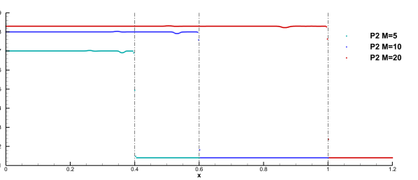
Figure 1: Numerical results obtained with our third $P_{2}$ (left) and fourth $P_{3}$ (right) order scheme for the planar shock wave propagation with Mach $M=5$ (dark-green), $M=10$ (blue) and $M=20$ (red). We also report with dashed black lines the expected position of each shock wave at the final time $t_{f}=0.04$ to show that our scheme perfectly deals with shock waves modeling.

5.1.3 Lax shock tube

We continue our set of Riemann problems by solving the Lax shock tube, originally due to [50], which in addition to one shock wave also develops a contact wave and a rarefaction fun. The initial conditions that originate the three waves are

$$(\rho,u,v,p)(\mathbf{x})=\begin{cases}(0.5,0,0,0.571)&\ \text{ if }\ x>0.5,\\ (0.445,0.698,0,3.528)&\ \text{ if }\ x\leq 0.5,\\ \end{cases}$$ (71)

and we solve this test problem on the domain $\Omega=[0,1]\times[0,0.1]$ up to the final time $t_{f}=0.14$. We report our numerical results compared with a reference solution in Figure 2, where we can notice that the conservative second order limiter is activated exactly where the shock wave is located which allows to perfectly track the shock position without any error on the computation of the shock speed.

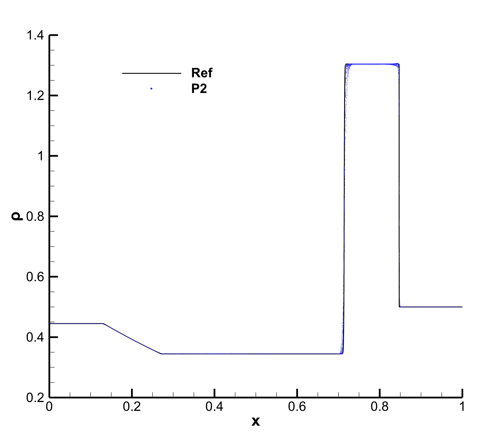
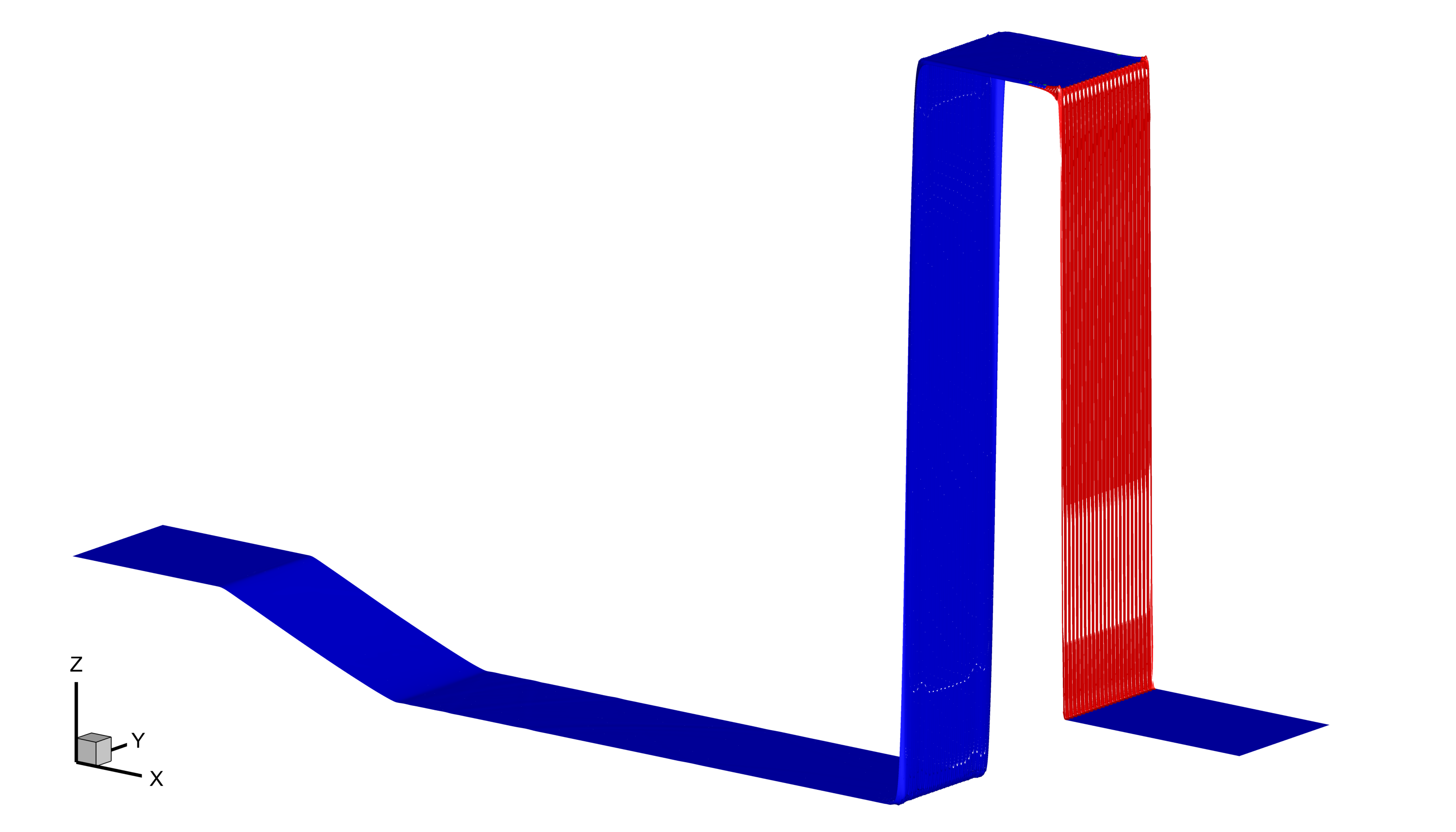
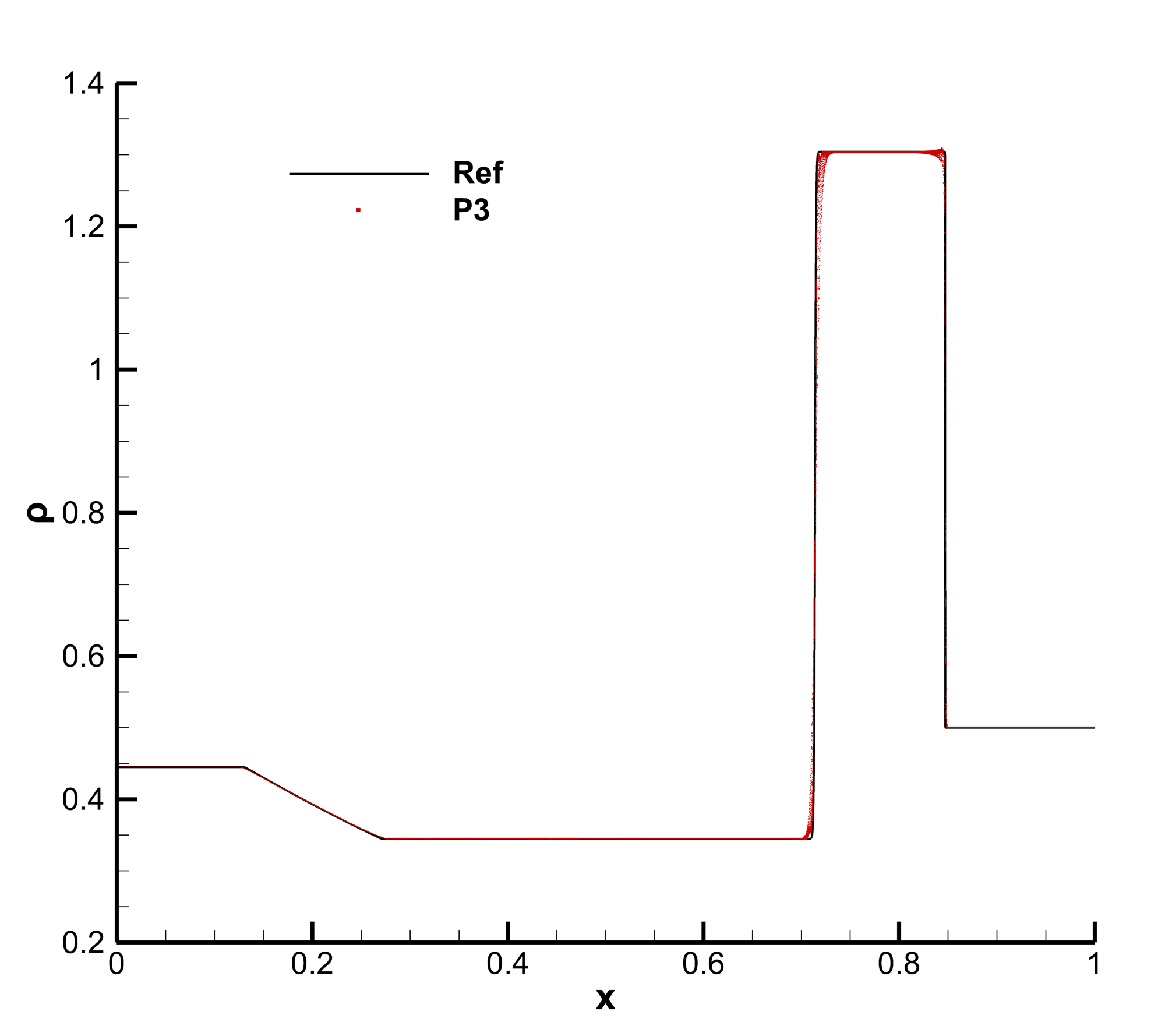
Figure 2: Lax shock tube solved on a polygonal tessellation with characteristic mesh size $h=1/430$. We report the results obtained with our quasi-conservative third order $P_{2}$ (top) and fourth order $P_{3}$ (bottom) schemes. In particular, we show on the left a graph whose $z-$coordinate is given by the density and whose colors refer to the type of scheme employed on each cell: blue for our quasi-conservative scheme, green for the second order limiter in primitive variables and red for the second order limiter applied on the conservative formulation, which is used to discretize the solution where the shock wave is located. Then, on the right, we report a scatter plot of our numerical results for the density profile compared with a reference solution obtained with a one dimensional Euler solver using a fully conservative explicit second order limited Residual Distribution scheme (see e.g. [59, 8]) on 50000 points.

5.1.4 Circular Sod explosion problem

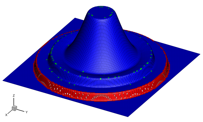
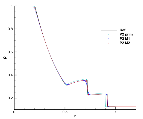
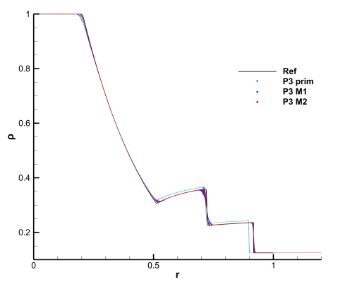
Figure 3: Circular Sod explosion. We show the numerical results obtained with our quasi-conservative third order $P_{2}$ (top row) and fourth order $P_{3}$ (bottom row) discontinuous Galerkin schemes. On the left, we depict in blue the cells where our DG scheme has been applied to the non-conservative formulation and in red or green those where our second order subcell FV limiter has been activated. In particular, on the red cells which correspond to shock-triggered troubled cells the FV schemes is applied on the conservative formulation of the Euler equations. On the right, we report the scatter plot of the numerical solution obtained on a coarse mesh $M_{1}$ with characteristic mesh size of $h=1/50$ and a finer one $M_{2}$ with characteristic mesh size of $h=1/215$, compared with a reference solution (black), and the incorrect solution (green) that one could have obtained by applying the DG scheme for the non-conservative formulation everywhere on the domain, including the shock regions.

This circular explosion problem can be seen as a multidimensional extension of the classical Sod test case. Here, we consider as computational domain a square of dimension $[-1;1]\times[-1;1]$, and the initial condition is composed of two different states, separated by a discontinuity at radius $r_{d}=0.5$

$$(\rho,u,v,p)(\mathbf{x})=\begin{cases}(1.0,0,0,1)&\ \text{ if }\ r\leq r_{d},\\ (0.125,0,0,0.1)&\ \text{ if }\ r>r_{d}.\\ \end{cases}$$ (72)

The final time is chosen to be $t_{f}=0.25$, so that the shock wave does not cross the external boundary of the domain, where wall boundary conditions are imposed. We have obtained a reference solution thanks to the rotational symmetry of the problem which reduces to a one-dimensional problem with geometric source terms, which we have solved by using a classical second order TVD scheme on a very fine mesh. In Figure 3, we report the numerical results obtained with our third and fourth order quasi-conservative schemes, compared both with a reference solution and the wrong results that one could obtain by working with the primitive formulation of the Euler equations everywhere on the domain. Indeed, with our approach on the shock regions (depicted in red in Figure 3), instead of using the original scheme, we apply our second order limiter scheme acting on the conservative formulation, and it is evident that this local switch is enough to restore the ability of the scheme to correctly capture the propagation speed of shockwaves.

5.1.5 Woodward-Colella blast wave

The last Riemann problem that we consider is the so-called Woodward and Colella blast wave due to [73]. This test case is a standard low energy benchmark problem and it is characterized by the interaction of two strong shocks that reach the boundaries and are further reflected so to produce additional mutual interactions. The initial data is built as follow

$$(\rho,u,v,p)(\mathbf{x})=\begin{cases}(1,0,0,1000)&\ \text{ if }\ 0\leq x\leq 0.1,\\ (1,0,0,10^{-2})&\ \text{ if }\ 0.1<x\leq 0.9,\\ (1,0,0,10^{2})&\ \text{ if }\ 0.9<x\leq 1.0,\\ \end{cases}$$ (73)

and the problem is solved on the rectangular domain $\Omega=[0,1]\times[0,0.1]$

We report our numerical results in Figure (4): in particular, we depict in red the shock-triggered troubled cells and we compare the scatter plot of the solution obtained with our quasi-conservative schemes with a reference solution obtained with a fully conservative one dimensional explicit second order limited Residual Distribution scheme (see e.g. [59, 8]) on 50000 points. In addition to the correct detection of all the generated waves and the correct location of shocks, convergence can be noticed by comparing visually the results obtained with our third and fourth order schemes.

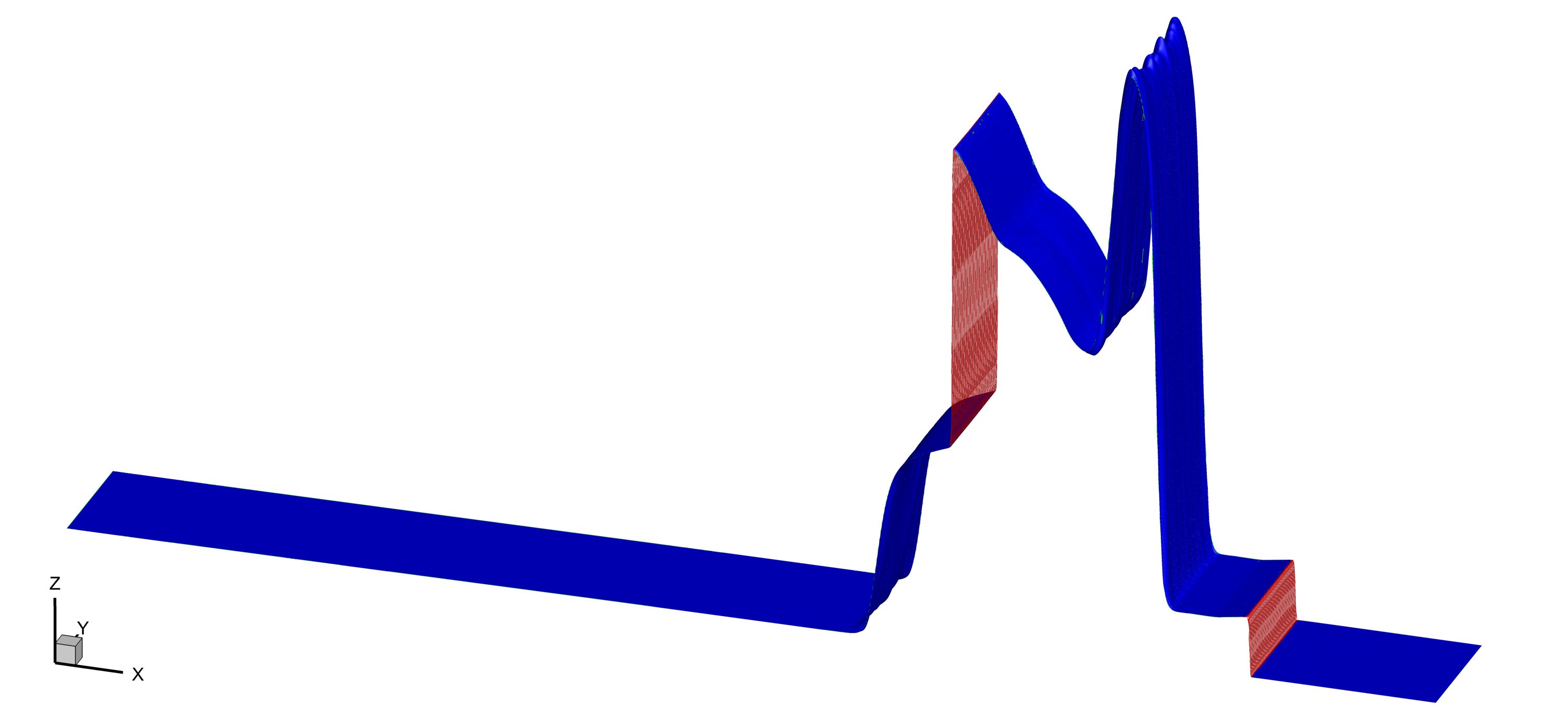
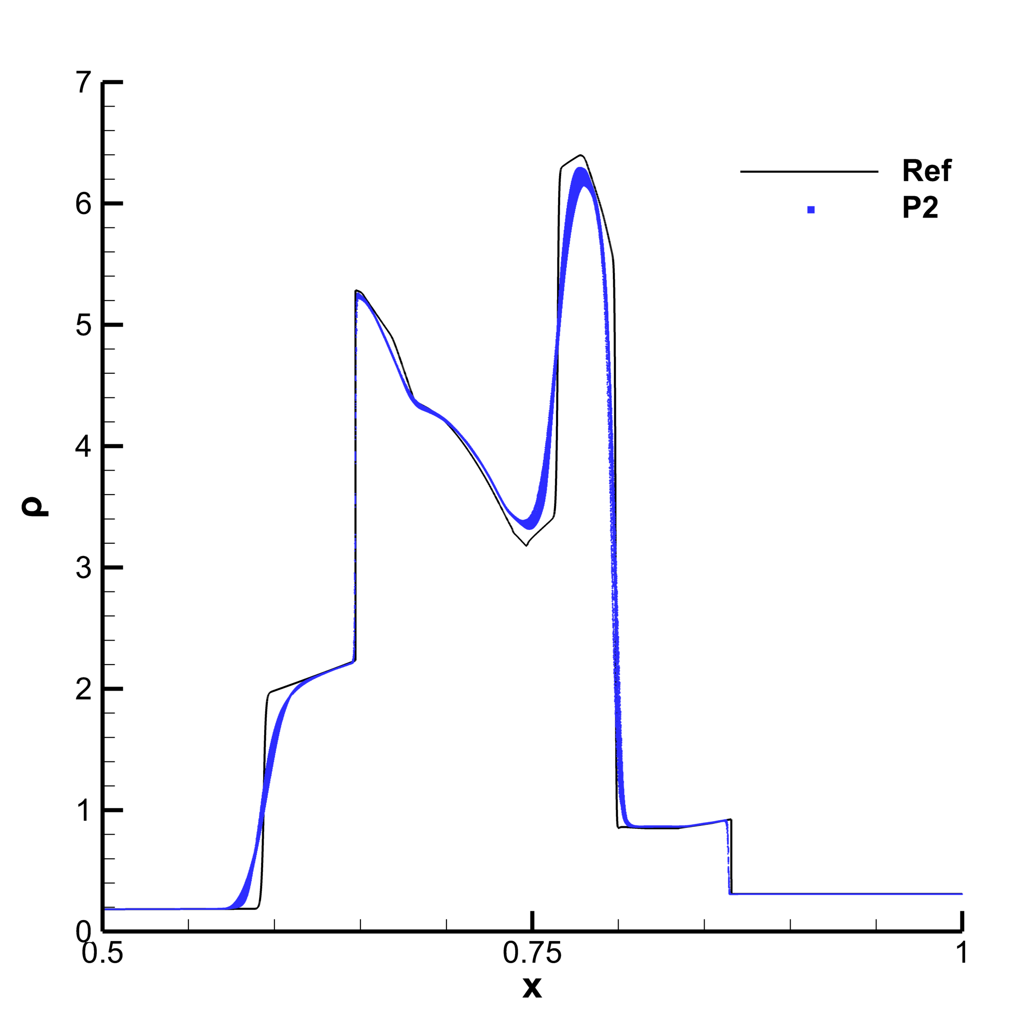
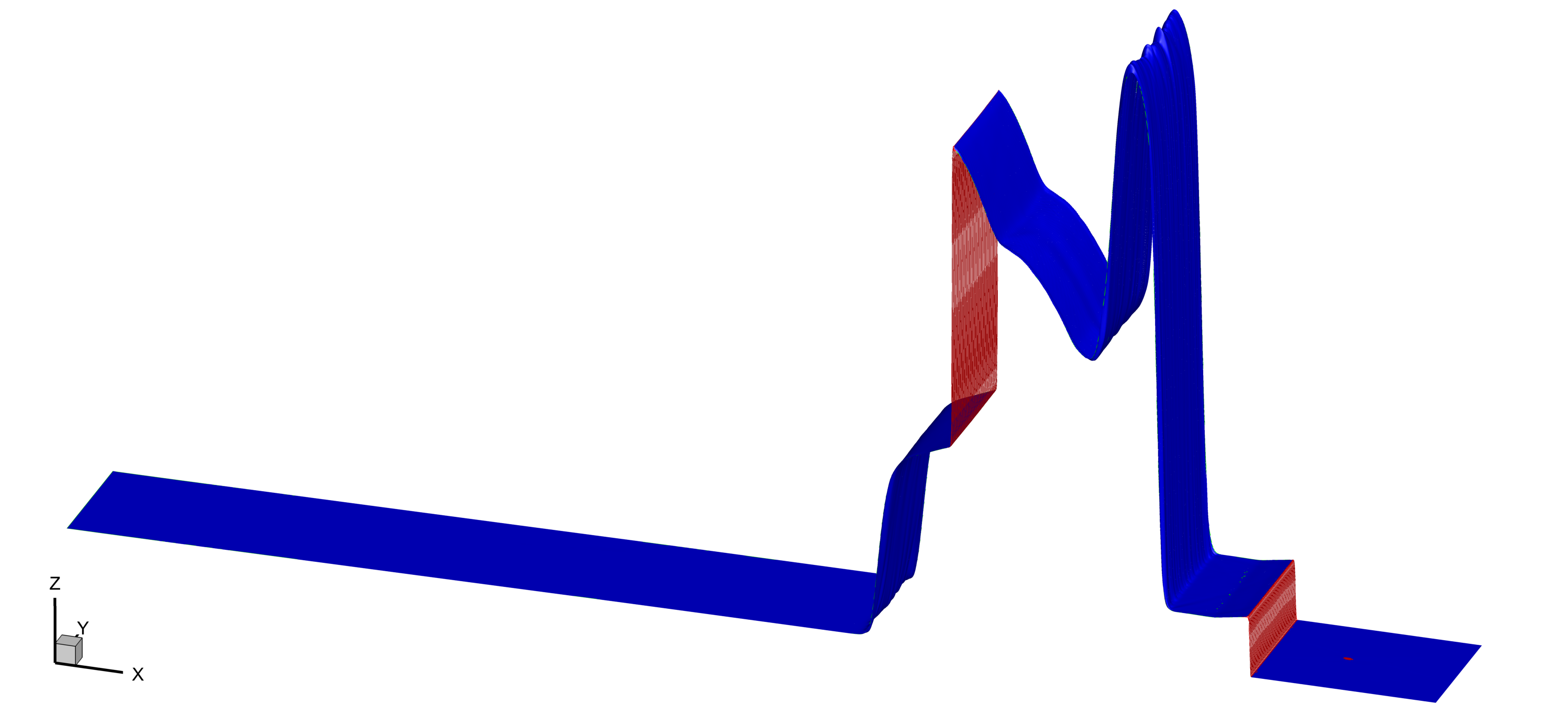
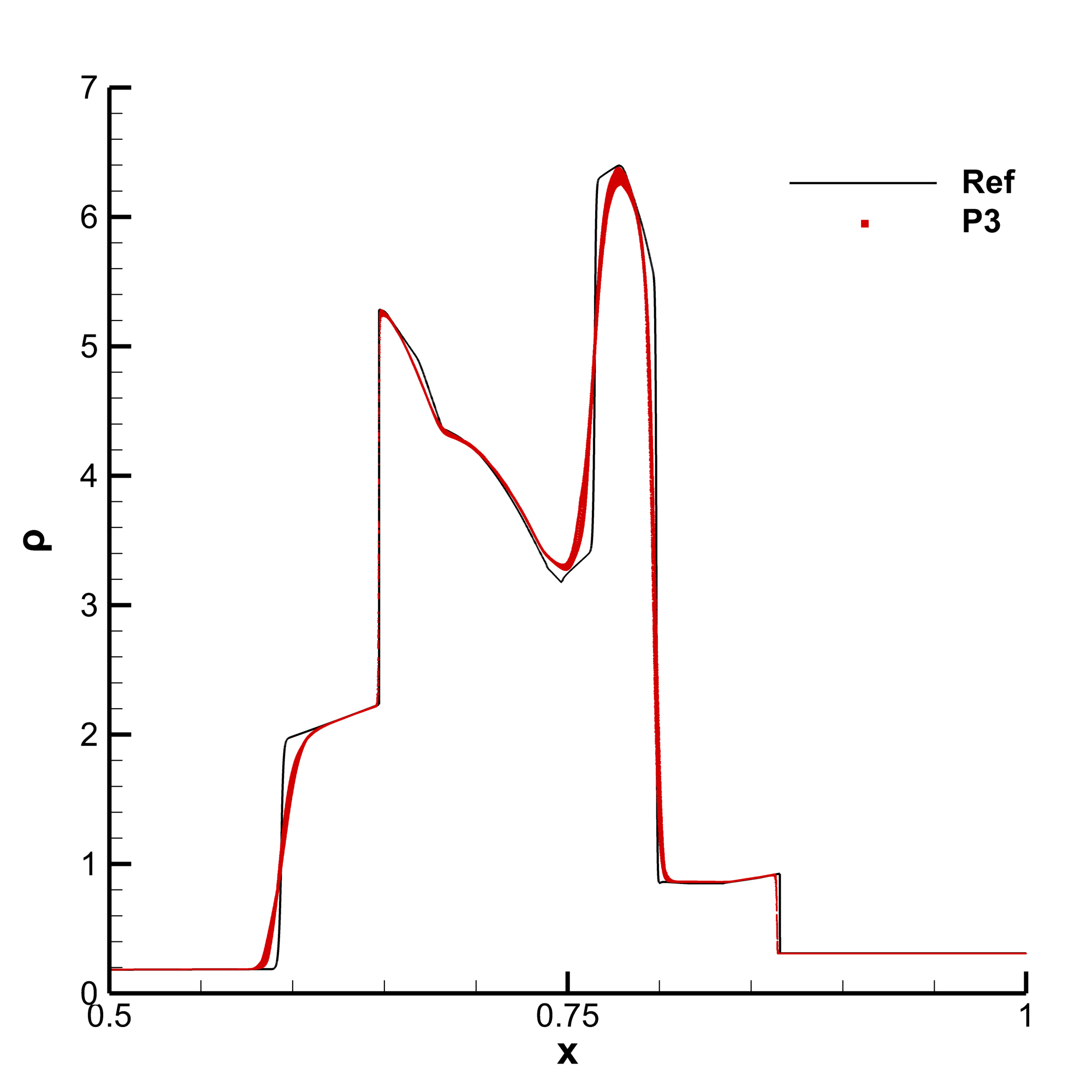
Figure 4: Woodward-Colella blast waves at the final time $t=0.038$ solved on a polygonal tessellation with characteristic mesh size $h=1/1080$. We report the results obtained with our third order $P_{2}$ (top row) and fourth order $P_{3}$ (bottom row) discontinuous Galerkin schemes, which solve the Euler equations formulated in primitive variables everywhere a part for the shock regions, highlighted in red on the left, where a second order FV scheme has been applied to the conservative formulation of the PDE at the subgrid level. In particular, on the right we report a zoom on the region $x\in[0.5,1]$ where we compare the scatter plot of our numerical results with a reference solution obtained with a fully conservative non-linear Residual Distribution scheme [59, 8] applied to the 1D Euler equations on 50000 points.

5.1.6 Forward Facing Step

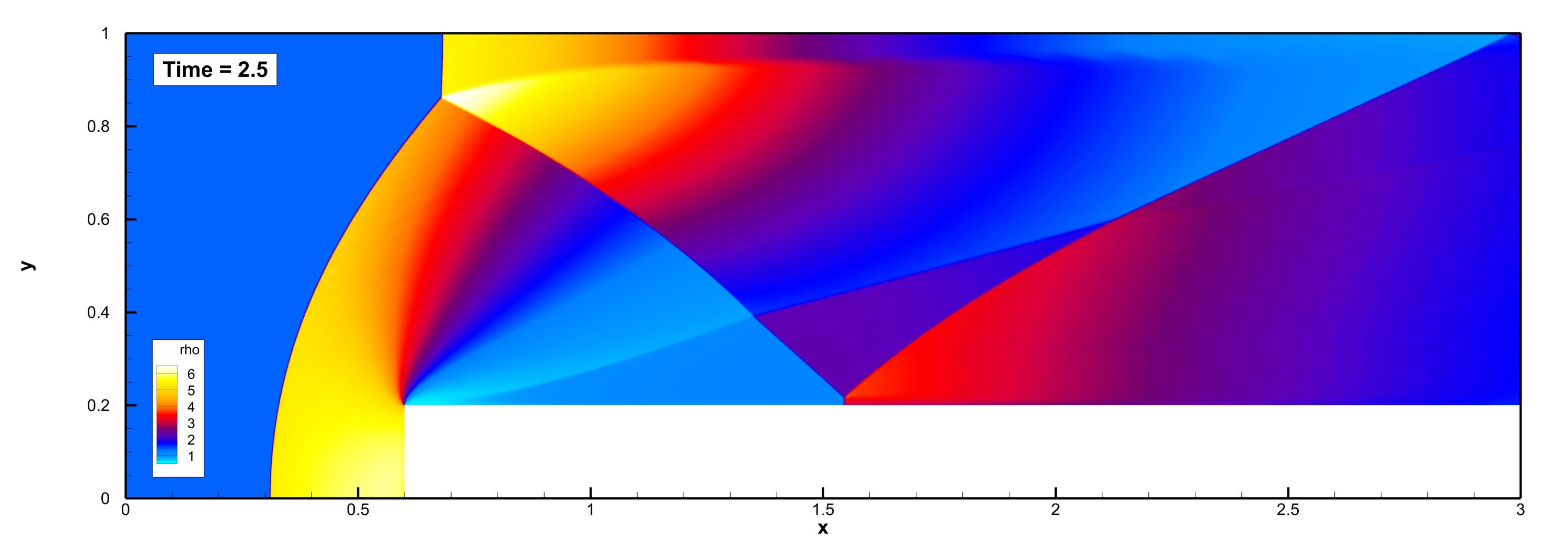
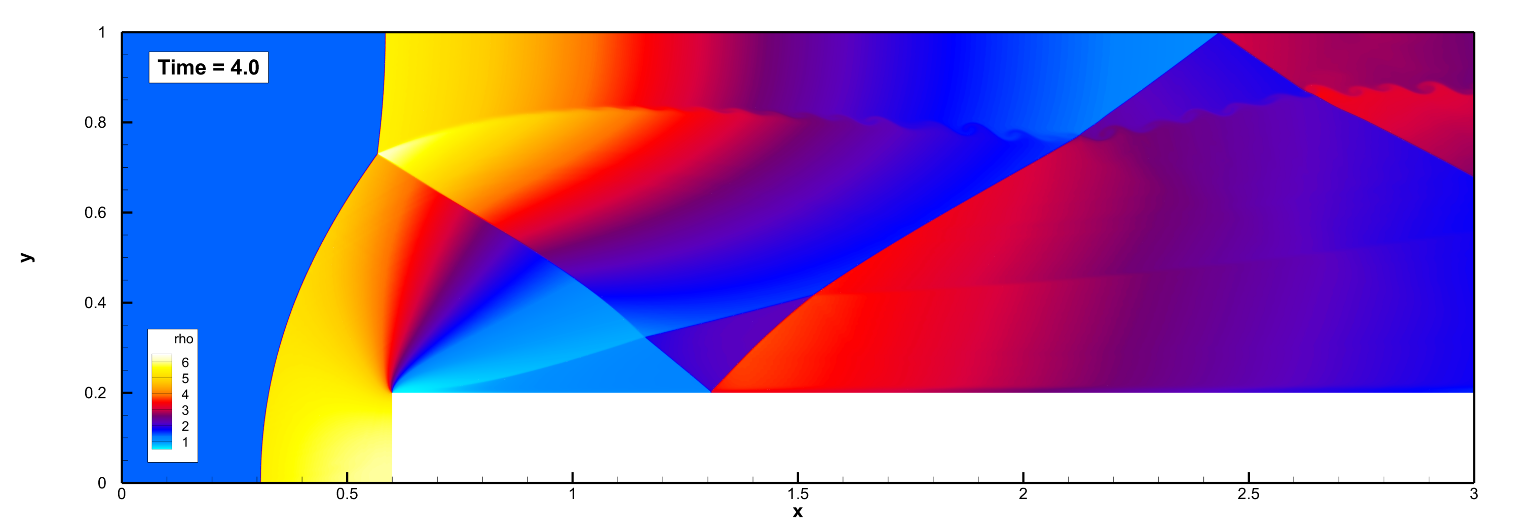
Figure 5: Numerical results for the forward facing step benchmark at time $t=2.5$ and $t=4$ obtained with our quasi-concervative third order $P_{2}$ (first and third image) and fourth order $P_{3}$ (second and fourth image) DG schemes on a polygonal tessellation with characteristic mesh size of $h=1/80$.

We now consider the forward facing step problem which is a truly two-dimensional test case to be studied on a non trivial domain composed as follow $\Omega=[0,7]\times[0,3]-[0.6,7]\times[0,0.2]$. This challenging benchmark has been introduced in [32] and further studied by Woodward and Colella in [73]. The problem begins with uniform Mach 3 flow in a wind tunnel containing a step. The initial density of the tunnel is $rho_{0}=\gamma=1.4$ and the initial pressure is $p_{0}=1$. For what concerns boundary conditions the exit right boundary has no effect on the flow, because the exit velocity is always supersonic. On the other side of the domain the gas is continually fed in from the left-hand boundary by setting the left ghost state always equal to the initial conditions. Finally, wall boundary conditions are set on the bottom and top part of the domain. We report the numerical results obtained with our third order $P_{2}$ and fourth order $P_{3}$ quasi-conservative DG scheme in Figure 5 at time $t=2.5$ and $t=4.0$.

5.1.7 Double Mach Reflection

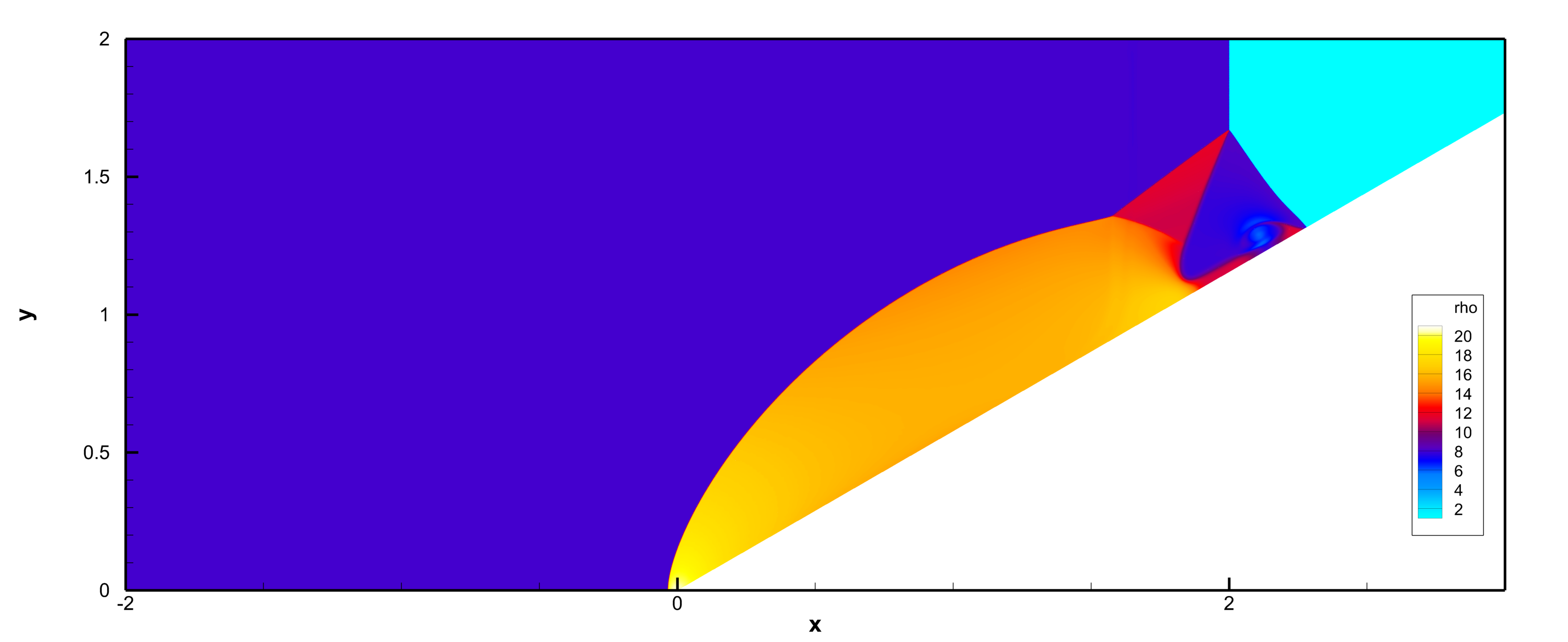
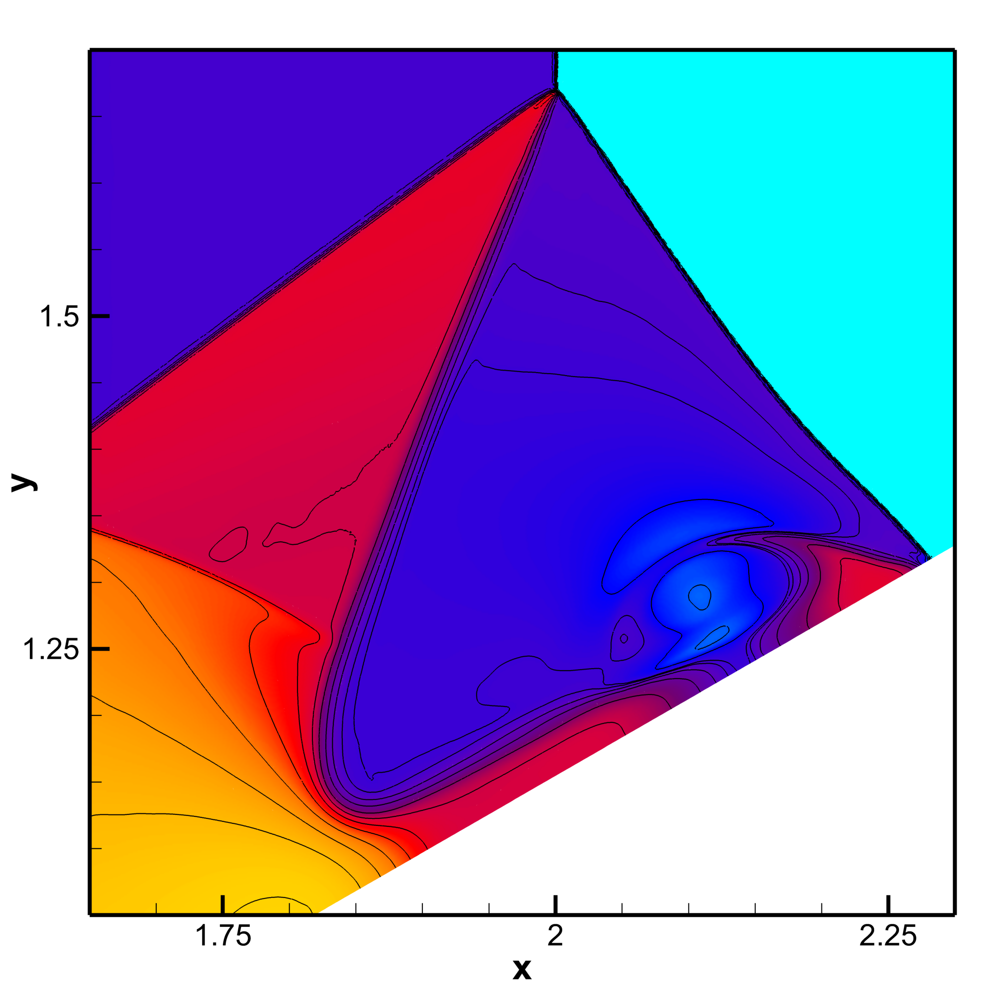
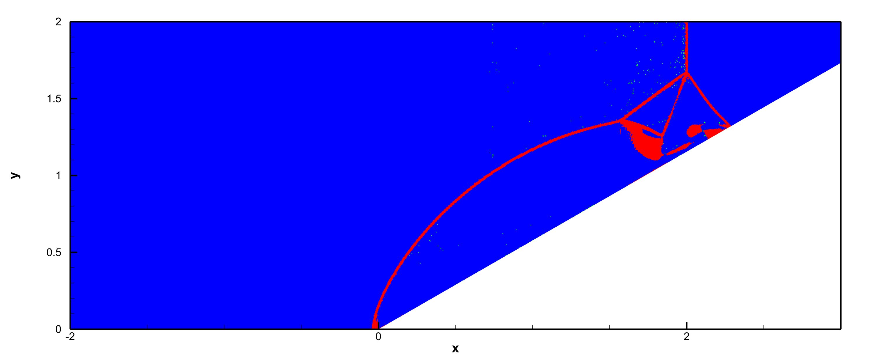
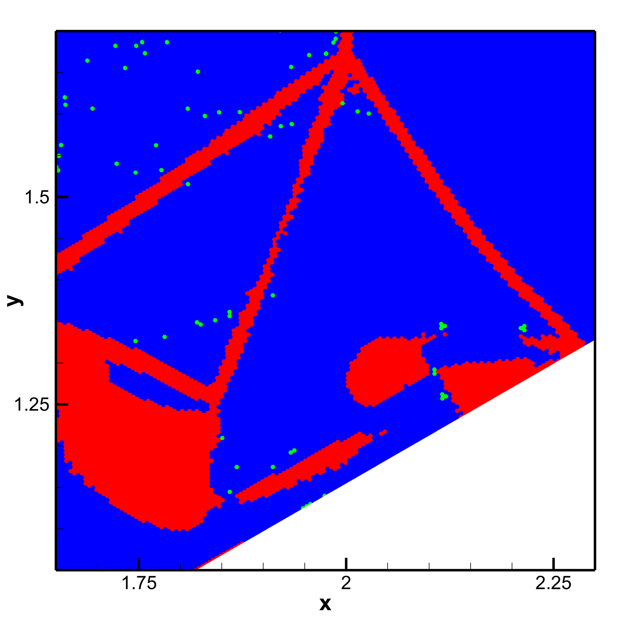
Figure 6: Numerical results for the Double Mach Reflection at time $t_{f}=0.2$ obtained with our quasi-concervative third order $P_{2}$ discontinuous Galerkin scheme on a polygonal tessellation with characteristic mesh size of $h=1/220$: density (top) and limiter type (bottom).

We close our set of validating benchmarks with the double Mach reflection problem which also has been originally proposed by Woodward and Colella in [73], where it has been studied on a rectangular domain thanks to a rotation of the initial conditions. Here, since we employ unstructured meshes, the problem can be directly run in physical coordinates as done in [28] by considering as computational domain the polygon obtained by connecting the points $(-2,0)-(0,0)-(3,\sqrt{3})-(3,2)-(-2,2)$. We consider a very strong shock wave that is moving along the x-direction at Mach $M=10$ and impacting against the ramp of angle $\pi/6$. The initial condition is given by

$$(\rho,u,v,p)(\mathbf{x})=\begin{cases}(8,8.25,0,116.5)&\ \text{ if }\ x\leq 0,\\ (\gamma,0,0,1)&\ \text{ if }\ x>0,\\ \end{cases}$$ (74)

with $\gamma=1.4$ and the final computational time is $t_{f}=0.2$. The strong shock wave that hits the ramp causes the development of other two shock waves, one traveling towards the right and the other one propagating towards the top boundary of the domain. The results obtained with our quasi-conservative third order $P_{2}$ DG scheme on a polygonal tessellation with characteristic mesh size $h=1/220$, are depicted in Figure 6. The small-scale structures produced by the roll-up of the shear layers behind the shock wave are clearly visible from the density contour lines for which also a zoom is provided on the right part of the Figure. Moreover, we depict in red the shock-triggered troubled cells which are treated by the a posteriori subcell limiter with the conservative correction, and in green the other limited cells treated instead in primitive variables. The use of the conservative formulation just on the shock regions allows to correctly reproduce the dynamics of this benchmark, while the majority of the domain can still be simulated in primitive variables.

5.2 Euler equations with space-time-dependent EOS parameters

5.2.1 Quirk and Karni’s test case

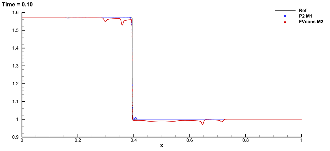
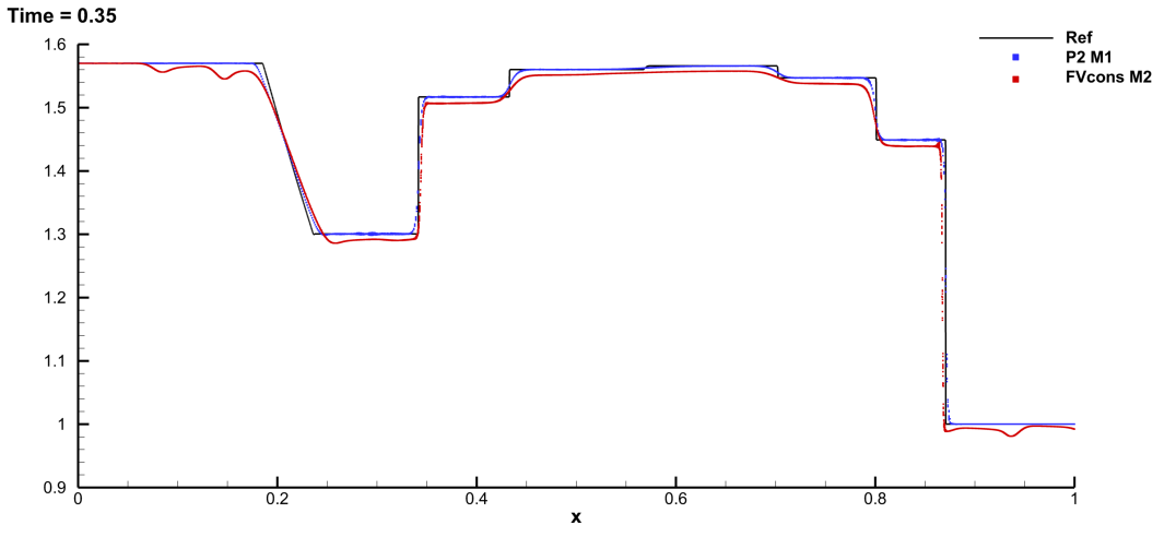
Figure 7: Pressure profile for the essentially 1D Quirk and Karni’s test case at time $t=0.1$, i.e. just before the shock hits the 1D-bubble, and at the final time $t=0.35$. We compare the numerical results obtained with our third order $P_{2}$ quasi-conservative DG scheme on a polygonal tessellation with characteristic mesh size $h=1/270$ (blue) with those obtained with a standard conservative second order FV scheme on a fine triangulation with $h=1/2690$ (red); we also provide a reference solution (black solid line). The solution obtained with the classical conservative scheme, even if run on a very fine mesh, develops spurios pressure oscillations already before the shock wave has hit the bubble which are then propagated around the domain and corrupt the solution.

We start with an essentially one-dimensional test case first proposed by Quirk and Karni in [57] and further investigated by Abgrall in [2]. This 1D test case mimics the shock helium-bubble interaction, that we also study in the two-dimensional setting in the next Section, and shares with it the difficulties of multi-material simulations. Indeed a classical simulation performed by using the conservative formulation (8) produces spurious oscillations that corrupt the final solution as clearly shown by the red graphs in Figure 7.

The initial setting for this problem is the following

$$(\rho,u,v,p,c)(\mathbf{x})=\begin{cases}(1.3765,0.3948,0,1.57,1)&\ \text{ if }\ x\leq 0.2,\\[2.0pt] (0.138,0,0,1,\frac{5}{3\gamma})&\ \text{ if }\ 0.4\leq x\leq 0.6,\\[2.0pt] (1,0,0,1,1,1)&\ \text{{ otherwise}},\end{cases}$$ (75)

on a rectangular domain $\Omega=[0,1]\times[0,0.05]$ with Dirichlet boundary conditions at the left and right borders and wall boundary conditions on the bottom and top edges. We have reported the numerical results obtained with our $P_{2}$ quasi-conservative approach in Figure 7 which perfectly agree with the reference solutions we have obtained by solving Kapila’s model [43] for one-velocity one-pressure compressible mutiphase flow (also known as five-equation Baer–Nunziato system [10]) on a very fine mesh of 20000 uniform cells by means of a second order path-conservative ADER-FV method with TVD reconstruction, specifically the one presented and validated in [24, 23].

5.2.2 Shock helium-bubble interaction

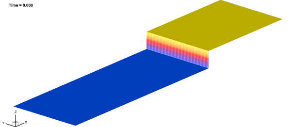
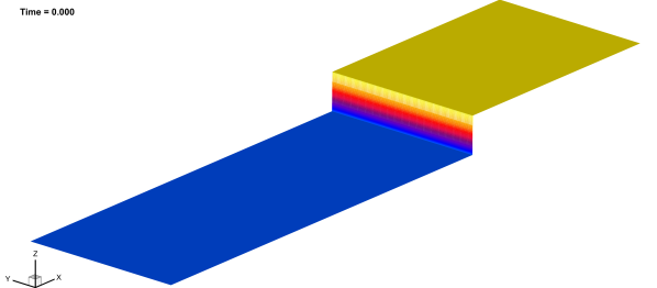
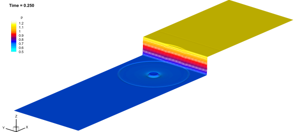
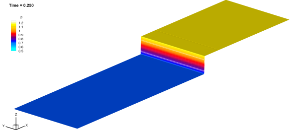
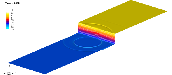
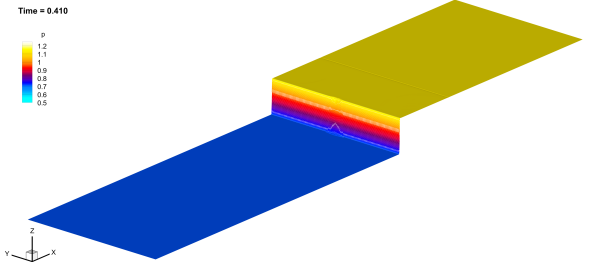
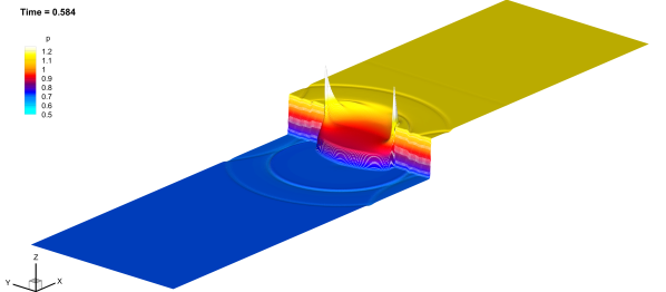
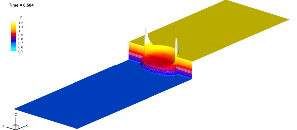
Figure 8: Pressure profile for the shock helium-bubble interaction. In this first figure, we compare the numerical results obtained with our third order $P_{2}$ quasi-conservative DG scheme on a polygonal tessellation with characteristic mesh size $h=1/150$ (right) with those obtained with a robust second order conservative ENO finite volume scheme on a very fine triangular mesh with $h=1/750$ (left). We remark that the second order FV scheme used here for comparison reasons, produces spurious oscillations which propagate away from the interface between the air and the bubble, in the form of circular pressure waves. Instead, our quasi-conservative approach, by working in primitive variables in particular at the bubble interface (see also next figure), completely avoids any spurious oscillations. Since both schemes employ at the limiter level the same ENO reconstruction, it is clear that the oscillations are induced by the conservative fluxes at material interfaces and not related to Gibbs-like oscillations.

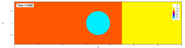
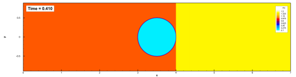
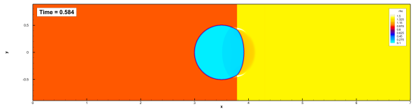
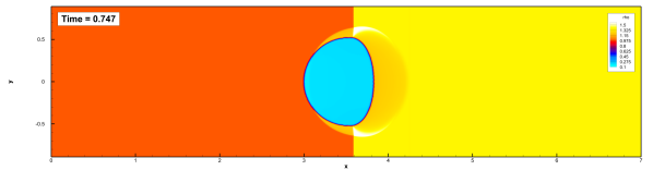
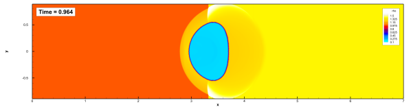
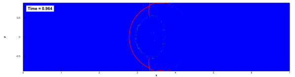
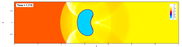
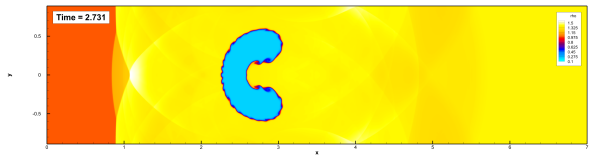
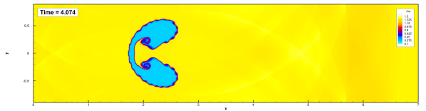
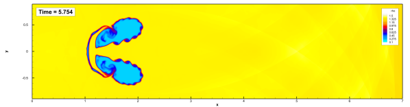
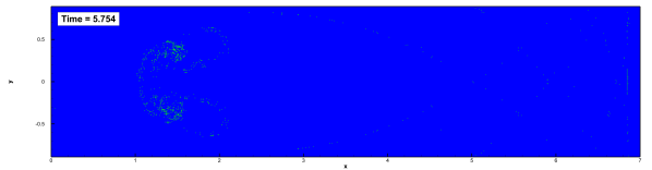
Figure 9: Shock helium-bubble interaction: on the left, we report the density profile obtained with our $P_{2}$ quasi-conservative scheme, and on the right, the distribution of limiter activations and the type of detected troubled cells. We emphasize that the limiter activates both at the discontinuity produced by the bubble-air interface and the shock wave; however it works with the conservative formulation of the PDE (8) only on the shock-triggered troubled cells (depicted in red), thus without negatively affecting the oscillation-free solution given by the primitive formulation at the material interface. The figure shows the initial condition (first line) and the dimensionless time $T^{*}=0.41$ ($t^{*}=75$ [$\mu$s]), when the shock first impacts onto the bubble (second line). The other output times correspond to the physical times $t=t^{*}+[32,62,102,240,427,674,983]$ [$\mu$s].

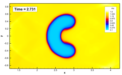
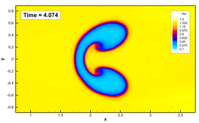
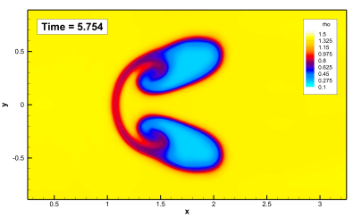
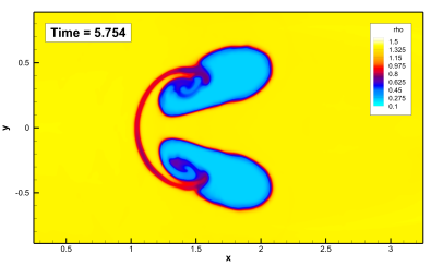
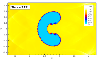
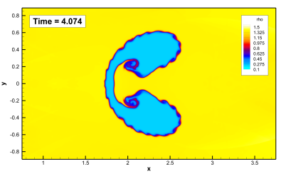
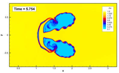
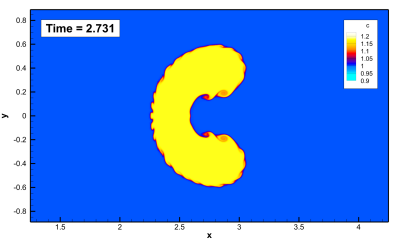
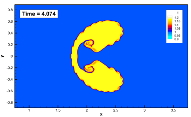
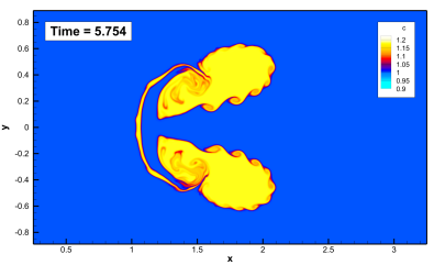
Figure 10: Mesh convergence of the main flow structures for the shock helium-bubble interaction. In this figure we report the density profile (first three lines) and the values of $c$ (last line) at three output times $t=2.731$, $t=4.074$, $t=5.754$. In particular, we have used three polygonal tessellations with characteristic mesh size $h=1/30$ (first line), $h=1/75$ (second line) and $h=1/150$ (third and fourth line).

Finally, we investigate the two-dimensional dynamics of the shock–bubble interaction. We consider a rectangular computational domain of size $[0,7D]\times[-0.89D,0.89D]$ filled with air, with $D$ being a spatial dimensionless parameter. A shock wave of Mach $M=1.22$ is located at $x=4.5D$ and is traveling from right to left, and it will hit a helium bubble of radius $r_{b}=0.05$ and center $(3.5D,\,0)$. The time coordinate $t$ can be also made non-dimensional using the shock velocity and the radius of the bubble, thus obtaining the dimensionless time $T=t/(r_{b}/c\,M)$, where $c_{a}=\sqrt{\gamma p_{a}/\rho_{a}}$ is the sound speed of the air. The pre-shock conditions in the air are

$$(\rho,u,v,p,c)(\mathbf{x})=\left(1,0,0,\frac{1}{\gamma},1\right),$$ (76)

with $\gamma=1.4$, and the post-shock conditions are

$$(\rho,u,v,p,c)(\mathbf{x})=\left(1.3764,-0.3336,0,\frac{1.5698}{\gamma},1\right).$$ (77)

The initial conditions inside the helium bubble are

$$(\rho,u,v,p,c)(\mathbf{x})=\left(0.1819,0,0,\frac{1}{\gamma},\frac{1.648}{\gamma}\right).$$ (78)

The dimensional quantities adopted for the simulation are computed by considering $D=1$ [m], $c_{a}=331.6$ [m/s], $p_{a}=101325$ [Pa] and $\rho_{a}=1.29\cdot 10^{-3}$ [kg/m³]. For what concerns boundary conditions, we impose the wall type on the top and bottom side of the domain and Dirichlet on the left and right parts.

This test case corresponds to the experiment of Hass and Sturtevant reported in [38]. It involves shock waves, material interfaces and their interaction and has been used by several researchers [44, 57, 2, 7, 53, 64], and more recently in [48, 39, 40], to demonstrate the capability of their numerical schemes in the simulation of compressible multi-component flows.

The output times are chosen according to the experimental setup in [38] and the numerical results of [46], hence we consider the series of physical times $t=t^{*}+[32,62,102,240,427,674,983]$ [$\mu$s], which correspond to the dimensionless times $T=T^{*}+[0.584,0.747,0.964,1.714,2.731,4.074,5.754]$. The shock wave hits the bubble at time $T^{*}=0.410$ ($t^{*}=75$ [$\mu$s]), that is also shown in the results. We report the results obtained with our third order $P_{2}$ quasi-conservative DG schemes in Figures 8, 9 and 10. In particular, in Figure 8 we compare our results with those one can obtain with a standard conservative second order finite volume scheme on a fine mesh to demonstrate that when working with the conservative PDE formulation (8) the scheme produces spurious pressure oscillations at the material interface, while our approach completely avoids these spurious waves. Then, in Figure 9 we show the cells where the limiter have been activated at various output times, and we differentiate between the shock-triggered troubled cells (depicted in red), where we work in conservative variables, by the activations due to the discontinuities of $\rho$ and $c$ at the material interface (depicted in green) which are treated with our a posteriori subcell limiter but still employing the non-conservative formulation (14). Finally, in Figure 10 we show the results obtained with successive mesh refinements to provide a visual convergence of the main flow structures.

6 Conclusions

In this paper we have discussed a new approach to efficiently use the non-conservative form of non-linear hyperbolic systems, while retaining a correct approximation of shocks. The method is based on a clever combination of a non-conservative fully explicit ADER-DG method, with a posteriori subcell corrections which include both a subcell limited update and a subcell correction to remove the conservation defect. The two corrections are activated by appropriately defined cell markers, which may flag cells as either troubled or shock activated troubled cells (or both). To provide some theoretical justification to this correction, a framework is proposed to define the conservation defect associated to the fully non-conservative method. Conditions on this defect are given for a modified Lax-Wendroff theorem to hold. This has allowed to generalize to our approach known results concerning the approximation smooth flows, contact discontinuities, and material interfaces, while justifying the idea of removing such defect in shocks. In practice, the shock detection is performed using a sensor inspired by Lagrangian hydrodynamics. The method has been tested on a variety of problems going from smooth solutions, to very strong shocks, and shock-contact interactions showing excellent results.

Several extensions and enhancements of this work are possible. The first one is clearly the application to more complex models, with more involved thermodynamics. One issue with many such models for multi-material flows is that they often contain non-conservative terms. In this case the question arises on what would be the appropriate way to design the conservative correction. For some systems, enough information exist however to caracterize shocks, of even build exact Riemann solvers (see e.g. [6]). This can give some idea. Another point of enhancement is the detection of shocks, currently involving the free parameter $m_{1}$. Some reduction of the sensitivity to this parameter may come from combining the current scaled divergence sensor with smoothness indicator related to the regularity of the approximating polynomials, see e.g. [47], or using finer calibration based on cells clustering [78]. More involved definitions may also be explored as e.g. those used in [62] for hypersonic flows.

Other extensions are interesting and open technical challenges as e.g. Lagrangian approximations, to further improve the approximation of contacts, or implicit explicit time stepping, to improve efficiency in presence of stiff thermodynamics (e.g. large variations of speed of sounds in different materials).

Appendix A Proof of Proposition 2

Proposition 2 claims that under the smoothness hypothesis (59) the conservation defect associated to the fully non-conservative formulation (32) verifies the conditions of Proposition 1. To demonstrate this estimate, we proceed as follows. First, we note that the continuity of the polynomial bases used for the approximation and the mean value theorem allow to write for the average of the primitive variables as

$$\bar{\mathbf{v}}_{i}=\mathbf{v}_{h}(\mathbf{x}^{*}_{i})$$

for some point $\mathbf{x}^{*}_{i}\in\omega_{i}$. By virtue of the smoothness assumption (59) we thus have in each cell

$$\mathbf{v}_{h}(\mathbf{x})-\bar{\mathbf{v}}_{i}=\mathcal{O}(h).$$

Using again (59) as well as (60) we can estimate the terms in the corrector step as

$$\int_{t^{n}}^{t^{n+1}}\int_{\omega_{i}}\phi_{k}\mathbf{H}d\mathbf{x}dt=\mathcal{O}(\Delta t\times h^{2})\;,\quad\int_{t^{n}}^{t^{n+1}}\int_{\partial\omega_{i}}\phi_{k}\mathbf{D}\cdot\mathbf{n}dSdt=\mathcal{O}(\Delta t\times h\times h)$$

which allows to state that for all degrees of freedom

$$\hat{\mathbf{v}}_{\ell}^{n+1}-\hat{\mathbf{v}}_{\ell}^{n}\leq\mathcal{O}\left(1/\int_{\omega_{i}}\phi_{\ell}\phi_{m}d\mathbf{x}\right)\;C\Delta t\,h^{2}=\mathcal{O}(\Delta t)=\mathcal{O}(h),$$

having used the time step definition (21) in the last equality.

We now estimate the variation of the local cell averages combining (52) and (6) as

$$\dfrac{\bar{\mathbf{q}}_{i}^{n+1}-\bar{\mathbf{q}}_{i}^{n}}{\Delta t}= \,\dfrac{1}{|\omega_{i}|}\dfrac{1}{\Delta t}\left(\,\int\limits_{\omega_{i}}\mathbf{T}^{-1}\left(\mathbf{v}_{h}^{n},\mathbf{v}_{h}^{n+1}\right)\left(\mathbf{v}_{h}^{n+1}-\mathbf{v}_{h}^{n}\right)d\mathbf{x}\right)$$

$$= \,\dfrac{1}{|\omega_{i}|}\dfrac{1}{\Delta t}\left(\,\int\limits_{\omega_{i}}\mathbf{T}^{-1}\left(\tilde{\mathbf{v}}_{h}^{n}(\mathbf{x}^{*}),\tilde{\mathbf{v}}_{h}^{n+1}(\mathbf{x}^{*})\right)\left(\tilde{\mathbf{v}}_{h}^{n+1}-\tilde{\mathbf{v}}_{h}^{n}\right)d\mathbf{x}\right)$$

$$+\,\dfrac{1}{|\omega_{i}|}\dfrac{1}{\Delta t}\left(\,\int\limits_{\omega_{i}}\left(\mathbf{T}^{-1}(\mathbf{v}_{h}^{n},\mathbf{v}_{h}^{n+1})-\mathbf{T}^{-1}\left(\tilde{\mathbf{v}}_{h}^{n}(\mathbf{x}^{*}),\tilde{\mathbf{v}}_{h}^{n+1}(\mathbf{x}^{*})\right)\right)\left(\tilde{\mathbf{v}}_{h}^{n+1}-\tilde{\mathbf{v}}_{h}^{n}\right)d\mathbf{x}\right).$$

Further, using the estimate on $\mathbf{v}_{h}-\bar{\mathbf{v}}_{i}$, the continuity properties (7) and the definition of $\mathbf{x}_{i}^{*}$ we can write

$$\dfrac{\bar{\mathbf{q}}_{i}^{n+1}-\bar{\mathbf{q}}_{i}^{n}}{\Delta t}=(\bar{\mathbf{T}}^{n+1/2})^{-1}\dfrac{\bar{\mathbf{v}}_{i}^{n+1}-\bar{\mathbf{v}}_{i}^{n}}{\Delta t}+C_{0}h$$

for some bounded constant $C_{0}$ depending on the mesh geometry and on the solution derivatives, and having set $(\bar{\mathbf{T}}^{n+1/2})^{-1}{\color[rgb]{0,0,0}:=}\mathbf{T}^{-1}(\bar{\mathbf{v}}_{i}^{n},\bar{\mathbf{v}}_{i}^{n+1})$. We can now use the update of the non-conservative corrector to see that

$$\dfrac{\bar{\mathbf{q}}_{i}^{n+1}-\bar{\mathbf{q}}_{i}^{n}}{\Delta t}=-\dfrac{1}{\Delta t}\dfrac{1}{|\omega_{i}|}\int_{t^{n}}^{t^{n+1}}\int_{\omega_{i}}\left(\bar{\mathbf{T}}^{n+1/2}\right)^{-1}\mathbf{H}(\tilde{\mathbf{v}}_{h})d\mathbf{x}\,dt-\dfrac{1}{\Delta t}\dfrac{1}{|\omega_{i}|}\int_{t^{n}}^{t^{n+1}}\int_{\partial\omega_{i}}\left(\bar{\mathbf{T}}^{n+1/2}\right)^{-1}\mathbf{D}\cdot\mathbf{n}\,dSdt+C_{0}h.$$ (79)

We can now manipulate the definition (53) as follows

$$\Phi_{i}= \sum\limits_{{\ell_{i,\alpha}}}\mathbf{F}_{\mathbf{n}_{{\ell_{i}}}}-\dfrac{1}{\Delta t}\int\limits_{t^{n}}^{t^{n+1}}\int\limits_{\partial\omega_{i}}\mathbb{F}(\tilde{\mathbf{v}}_{h}^{-})\cdot\mathbf{n}dS+\dfrac{1}{\Delta t}\int\limits_{t^{n}}^{t^{n+1}}\int\limits_{\partial\omega_{i}}\mathbb{F}(\tilde{\mathbf{v}}_{h}^{-})\cdot\mathbf{n}dS$$

$$= \sum\limits_{{\ell_{i}}}\mathbf{F}_{\mathbf{n}_{{\ell_{i}}}}-\dfrac{1}{\Delta t}\int\limits_{t^{n}}^{t^{n+1}}\int\limits_{\partial\omega_{i}}\mathbb{F}(\tilde{\mathbf{v}}_{h}^{-})\cdot\mathbf{n}dS+\dfrac{1}{\Delta t}\int\limits_{t^{n}}^{t^{n+1}}\int\limits_{\omega_{i}}\nabla\cdot\mathbb{F}(\tilde{\mathbf{v}}_{h}^{-})d\mathbf{x},$$

having assumed exact integration of the boundary terms so that the last term can be exactly expressed as a volume integral using the Gauss theorem. Consider the integrated numerical flux

$$\mathbf{F}_{\mathbf{n}_{i\ell}}=\dfrac{1}{2}\dfrac{1}{\Delta t}\int\limits_{t^{n}}^{t^{n+1}}\int\limits_{\partial\omega_{i}}\left(\mathbf{F}(\tilde{\mathbf{v}}_{h}^{+})+\mathbf{F}(\tilde{\mathbf{v}}_{h}^{-})\right)\cdot\mathbf{n}_{i\ell}-\dfrac{1}{2}\dfrac{1}{\Delta t}\int\limits_{t^{n}}^{t^{n+1}}\int\limits_{\partial\omega_{i}}\mathbf{T}^{-1}\left(\dfrac{\tilde{\mathbf{v}}_{h}^{+}+\tilde{\mathbf{v}}_{h}^{-}}{2}\right)\left|\mathsf{D}_{\mathbf{n}_{i\ell}}\right|(\tilde{\mathbf{v}}_{h}^{+}-\tilde{\mathbf{v}}_{h}^{-})$$ (80)

where

$$\dfrac{1}{2}\left|\mathsf{D}_{\mathbf{n}_{i\ell}}\right|:= \dfrac{1}{2}\int\limits_{0}^{1}\left|\left[\mathbf{A}_{\mathbf{V}}\left(\bm{\Psi}(\tilde{\mathbf{v}}_{h}^{-},\tilde{\mathbf{v}}_{h}^{+},s)\right),\ \mathbf{B}_{\mathbf{V}}\left(\bm{\Psi}(\tilde{\mathbf{v}}_{h}^{-},\tilde{\mathbf{v}}_{h}^{+},s)\right)\right]\cdot\mathbf{n}\right|ds$$

$$= \int\limits_{0}^{1}\dfrac{1}{2}\left[\mathbf{A}_{\mathbf{V}}\left(\bm{\Psi}(\tilde{\mathbf{v}}_{h}^{-},\tilde{\mathbf{v}}_{h}^{+},s)\right),\ \mathbf{B}_{\mathbf{V}}\left(\bm{\Psi}(\tilde{\mathbf{v}}_{h}^{-},\tilde{\mathbf{v}}_{h}^{+},s)\right)\right]\cdot\mathbf{n}\,ds-\mathsf{D}_{\mathbf{n}_{i\ell}}^{-},$$

having used the relation $(\cdot)^{-}=[(\cdot)-|\cdot|]/2$. Using this definition in the expression for $\Phi_{i}$ we can write

$$\Phi_{i{\alpha}}= \dfrac{1}{2}\dfrac{1}{\Delta t}\int\limits_{t^{n}}^{t^{n+1}}\int\limits_{\partial\omega_{i}}\left(\mathbb{F}(\tilde{\mathbf{v}}_{h}^{+})-\mathbb{F}(\tilde{\mathbf{v}}_{h}^{-})\right)\cdot\mathbf{n}dS-\dfrac{1}{2}\dfrac{1}{\Delta t}\int\limits_{t^{n}}^{t^{n+1}}\int\limits_{\partial\omega_{i}}\left(\bar{\mathbf{T}}^{n+1/2}\right)^{-1}\left|\mathsf{D}_{\mathbf{n}_{i\ell}}\right|(\tilde{\mathbf{v}}_{h}^{+}-\tilde{\mathbf{v}}_{h}^{-})dS+\dfrac{1}{\Delta t}\int\limits_{t^{n}}^{t^{n+1}}\int\limits_{\omega_{i}}\nabla\cdot\mathbb{F}(\tilde{\mathbf{v}}_{h}^{-})d\mathbf{x}$$

$$- \dfrac{1}{2}\dfrac{1}{\Delta t}\int\limits_{t^{n}}^{t^{n+1}}\int\limits_{\partial\omega_{i}}\bigg{(}\mathbf{T}^{-1}(\tilde{\mathbf{v}}_{h}^{-})-\left(\bar{\mathbf{T}}^{n+1/2}\right)^{-1}\bigg{)}\left|\mathsf{D}_{\mathbf{n}_{i\ell}}\right|(\tilde{\mathbf{v}}_{h}^{+}-\tilde{\mathbf{v}}_{h}^{-})dS-\dfrac{1}{2}\dfrac{1}{\Delta t}\int\limits_{t^{n}}^{t^{n+1}}\int\limits_{\partial\omega_{i}}\bigg{(}\mathbf{T}^{-1}\left(\dfrac{\tilde{\mathbf{v}}_{h}^{+}+\tilde{\mathbf{v}}_{h}^{-}}{2}\right)-\mathbf{T}^{-1}(\tilde{\mathbf{v}}_{h}^{-})\bigg{)}\left|\mathsf{D}_{\mathbf{n}_{i\ell}}\right|(\tilde{\mathbf{v}}_{h}^{+}-\tilde{\mathbf{v}}_{h}^{-})dS.$$

The last two terms can be estimated using the continuity of the Jacobians (7), combined with (59) as well as (60),

$$\dfrac{1}{\Delta t} \int\limits_{t^{n}}^{t^{n+1}}\int\limits_{\partial\omega_{i}}\bigg{(}\mathbf{T}^{-1}(\tilde{\mathbf{v}}_{h}^{-})-\left(\bar{\mathbf{T}}^{n+1/2}\right)^{-1}\bigg{)}\left|\mathsf{D}_{\mathbf{n}_{i\ell}}\right|(\tilde{\mathbf{v}}_{h}^{+}-\tilde{\mathbf{v}}_{h}^{-})dS=\mathcal{O}(|\partial\omega_{i}|\times h\times h)=\mathcal{O}(h^{3}),$$

$$\dfrac{1}{\Delta t} \int\limits_{t^{n}}^{t^{n+1}}\int\limits_{\partial\omega_{i}}\bigg{(}\mathbf{T}^{-1}\left(\dfrac{\tilde{\mathbf{v}}_{h}^{+}+\tilde{\mathbf{v}}_{h}^{-}}{2}\right)-\mathbf{T}^{-1}(\tilde{\mathbf{v}}_{h}^{-})\bigg{)}\left|\mathsf{D}_{\mathbf{n}_{i\ell}}\right|(\tilde{\mathbf{v}}_{h}^{+}-\tilde{\mathbf{v}}_{h}^{-})dS=\mathcal{O}(|\partial\omega_{i}|\times h\times h)=\mathcal{O}(h^{3}),$$

where we still do not account for possible quadrature errors in the boundary integrals. We now invoke the continuity of the flux $\mathbb{F}$, to use formally a mean value linearization of its Jacobian matrices such that

$$\left(\mathbb{F}(\tilde{\mathbf{v}}_{h}^{+})-\mathbb{F}(\tilde{\mathbf{v}}_{h}^{-})\right)\cdot\mathbf{n}=\bar{J}_{\mathbf{n}}(\tilde{\mathbf{v}}_{h}^{-},\tilde{\mathbf{v}}_{h}^{+})(\tilde{\mathbf{v}}_{h}^{+}-\tilde{\mathbf{v}}_{h}^{-})=\left\{\bar{\mathbf{T}}^{-1}(\tilde{\mathbf{v}}_{h}^{-},\tilde{\mathbf{v}}_{h}^{+})\left[\bar{\mathbf{A}}_{\mathbf{V}}(\tilde{\mathbf{v}}_{h}^{-},\tilde{\mathbf{v}}_{h}^{+}),\bar{\mathbf{B}}_{\mathbf{V}}(\tilde{\mathbf{v}}_{h}^{-},\tilde{\mathbf{v}}_{h}^{+})\right]\cdot\mathbf{n}\right\}(\tilde{\mathbf{v}}_{h}^{+}-\tilde{\mathbf{v}}_{h}^{-}).$$

We can again use (7), combined with (59)-(60) to obtain

$$\left(\mathbb{F}(\tilde{\mathbf{v}}_{h}^{+})-\mathbb{F}(\tilde{\mathbf{v}}_{h}^{-})\right)\cdot\mathbf{n}=\left\{(\bar{\mathbf{T}}^{n+1/2})^{-1}\int\limits_{0}^{1}\left[\mathbf{A}_{\mathbf{V}}\left(\bm{\Psi}(\tilde{\mathbf{v}}_{h}^{-},\tilde{\mathbf{v}}_{h}^{+},s)\right),\ \mathbf{B}_{\mathbf{V}}\left(\bm{\Psi}(\tilde{\mathbf{v}}_{h}^{-},\tilde{\mathbf{v}}_{h}^{+},s)\right)\right]\cdot\mathbf{n}\,ds\right\}(\tilde{\mathbf{v}}_{h}^{+}-\tilde{\mathbf{v}}_{h}^{-})+\mathcal{O}(h^{2}).$$

Combining all the previous expressions we can show that

$$\Phi_{i}= \dfrac{1}{2}\dfrac{1}{\Delta t}\int\limits_{t^{n}}^{t^{n+1}}\int\limits_{\partial\omega_{i}}\left(\mathbb{F}(\tilde{\mathbf{v}}_{h}^{+})-\mathbb{F}(\tilde{\mathbf{v}}_{h}^{-})\right)\cdot\mathbf{n}dS-\dfrac{1}{2}\dfrac{1}{\Delta t}\int\limits_{t^{n}}^{t^{n+1}}\int\limits_{\partial\omega_{i}}(\bar{\mathbf{T}}^{n+1/2})^{-1}|\mathsf{D}_{\mathbf{n}_{i\ell}}|(\tilde{\mathbf{v}}_{h}^{+}-\tilde{\mathbf{v}}_{h}^{-})dS+\dfrac{1}{\Delta t}\int\limits_{t^{n}}^{t^{n+1}}\int\limits_{\omega_{i}}\nabla\cdot\mathbb{F}(\tilde{\mathbf{v}}_{h}^{-})d\mathbf{x}$$

$$= \dfrac{1}{\Delta t}\int\limits_{t^{n}}^{t^{n+1}}\int\limits_{\partial\omega_{i}}(\bar{\mathbf{T}}^{n+1/2})^{-1}\mathbf{D}(\tilde{\mathbf{v}}_{h}^{+}-\tilde{\mathbf{v}}_{h}^{-})\cdot\mathbf{n}dS+\dfrac{1}{\Delta t}\int\limits_{t^{n}}^{t^{n+1}}\int\limits_{\omega_{i}}\nabla\cdot\mathbb{F}(\tilde{\mathbf{v}}_{h}^{-})d\mathbf{x}$$

$$= \dfrac{1}{\Delta t}\int\limits_{t^{n}}^{t^{n+1}}\int\limits_{\partial\omega_{i}}(\bar{\mathbf{T}}^{n+1/2})^{-1}\mathbf{D}(\tilde{\mathbf{v}}_{h}^{+}-\tilde{\mathbf{v}}_{h}^{-})\cdot\mathbf{n}dS+\dfrac{1}{\Delta t}\int\limits_{t^{n}}^{t^{n+1}}\int\limits_{\omega_{i}}\mathbf{T}^{-1}(\tilde{\mathbf{v}}_{h}^{-})\mathbf{H}(\tilde{\mathbf{v}}_{h}^{-})d\mathbf{x}$$

$$= \dfrac{1}{\Delta t}\int\limits_{t^{n}}^{t^{n+1}}\int\limits_{\partial\omega_{i}}(\bar{\mathbf{T}}^{n+1/2})^{-1}\mathbf{D}(\tilde{\mathbf{v}}_{h}^{+}-\tilde{\mathbf{v}}_{h}^{-})\cdot\mathbf{n}dS+\dfrac{1}{\Delta t}\int\limits_{t^{n}}^{t^{n+1}}\int\limits_{\omega_{i}}(\bar{\mathbf{T}}^{n+1/2})^{-1}\mathbf{H}(\tilde{\mathbf{v}}_{h}^{-})d\mathbf{x}+\mathcal{O}(h^{3}),$$

as long as the boundary quadrature is exact at least for linear polynomials, and having used again the regularity of the discrete solution and (7) to deduce the estimation $\|[(\bar{\mathbf{T}}^{n+1/2})^{-1}-\mathbf{T}^{-1}(\tilde{\mathbf{v}}_{h}^{-})]\mathbf{H}(\tilde{\mathbf{v}}_{h}^{-})\|=\mathcal{O}(h)$.

Comparing this last expression to (79), we readily deduce that

$$\Delta_{i}=\dfrac{\bar{\mathbf{q}}_{i}^{n+1}-\bar{\mathbf{q}}_{i}^{n}}{\Delta t}+\dfrac{1}{|\omega_{i}|}\Phi_{i}=\mathcal{O}(h)$$

which concludes the proof.

Appendix B Proof of Proposition 5

To prove the 3 statements we write the conservation defect and define a numerical flux that matches the variation of $\mathbf{Q}(\mathbf{v}_{h})$ in time up to appropriately small terms. We start by recalling that due to the hypotheses made on the non-conservative update we have that

$$\mathbf{v}_{h}^{n}=\left(\begin{array}[]{c}\rho^{n}_{h}\\ u_{0}+C_{u}(x)h^{1+\epsilon}\\ v_{0}+C_{v}(x)h^{1+\epsilon}\\ p_{0}+C_{p}(x)h^{1+\epsilon}\\ \chi_{h}^{n}\end{array}\right)\;\!,\quad\tilde{\mathbf{v}}_{h}=\left(\begin{array}[]{c}\tilde{\rho}_{h}\\ u_{0}+C_{u}(x)h^{1+\epsilon}\\ v_{0}+C_{v}(x)h^{1+\epsilon}\\ p_{0}+C_{p}(x)h^{1+\epsilon}\\ \tilde{\chi}_{h}\end{array}\right)\;\!,\quad\mathbf{v}_{h}^{n+1}=\left(\begin{array}[]{c}\rho^{n+1}_{h}\\ u_{0}+C_{u}(x)h^{1+\epsilon}\\ v_{0}+C_{v}(x)h^{1+\epsilon}\\ p_{0}+C_{p}(x)h^{1+\epsilon}\\ \chi_{h}^{n+1}\end{array}\right)\!,$$

where for simplicity we keep the constants independent of the time iteration (the proof is identical if different values are used). The second observation is that, due to the previous remarks and to the structure of the Jacobian matrices (14) and of their eigenvectors, at a given interface we have in (34)

$$\mathsf{D}_{\mathbf{n}}^{-}(\tilde{\mathbf{v}}_{h}^{+}-\tilde{\mathbf{v}}_{h}^{-})=\min(0,\boldsymbol{\mathsf{v}}_{0}\cdot\mathbf{n})\left(\begin{array}[]{c}\tilde{\rho}_{h}^{+}-\tilde{\rho}_{h}^{-}\\ 0\\ 0\\ 0\\ \tilde{\chi}_{h}^{+}-\tilde{\chi}_{h}^{-}\end{array}\right)+\mathcal{O}(h^{1+\epsilon}).$$

Similarly, we can show that

$$\mathbf{H}(\tilde{\mathbf{v}}_{h})=\boldsymbol{\mathsf{v}}_{0}\cdot\left(\begin{array}[]{c}\nabla\tilde{\rho}_{h}\\ 0\\ 0\\ 0\\ \nabla\tilde{\chi}_{h}\end{array}\right)+\mathcal{O}(h^{\epsilon})=\nabla\cdot(\boldsymbol{\mathsf{v}}_{0}\tilde{\mathbf{v}}_{h})+\mathcal{O}(h^{\epsilon}).$$

We now look at the definition of the conservation defect and evaluate the first term for the mass/momentum/energy equations. Using the definitions of the conservative variables and the equation of state presented in Section 2.1

$$\dfrac{1}{\Delta t}\dfrac{1}{|\omega_{i}|}\int_{\omega_{i}}\rho(\mathbf{v}_{h}^{n+1})d\mathbf{x}-\dfrac{1}{\Delta t}\dfrac{1}{|\omega_{i}|}\int_{\omega_{i}}\rho(\mathbf{v}_{h}^{n})d\mathbf{x}\,= \dfrac{\bar{\rho}_{i}^{n+1}-\bar{\rho}_{i}^{n}}{\Delta t}$$ (81)

$$\dfrac{1}{\Delta t}\dfrac{1}{|\omega_{i}|}\int_{\omega_{i}}\rho\boldsymbol{\mathsf{v}}(\mathbf{v}_{h}^{n+1})d\mathbf{x}-\dfrac{1}{\Delta t}\dfrac{1}{|\omega_{i}|}\int_{\omega_{i}}\rho\boldsymbol{\mathsf{v}}(\mathbf{v}_{h}^{n})d\mathbf{x}\,= \boldsymbol{\mathsf{v}}_{0}\dfrac{\bar{\rho}_{i}^{n+1}-\bar{\rho}_{i}^{n}}{\Delta t}+\mathcal{O}(h^{\epsilon})$$

$$\dfrac{1}{\Delta t}\dfrac{1}{|\omega_{i}|}\int_{\omega_{i}}\rho E(\mathbf{v}_{h}^{n+1})d\mathbf{x}-\dfrac{1}{\Delta t}\dfrac{1}{|\omega_{i}|}\int_{\omega_{i}}\rho E(\mathbf{v}_{h}^{n})d\mathbf{x}\,= \kappa_{0}\dfrac{\bar{\rho}_{i}^{n+1}-\bar{\rho}_{i}^{n}}{\Delta t}+p_{0}\dfrac{\bar{\lambda}_{i}^{n+1}-\bar{\lambda}_{i}^{n}}{\Delta t}+\mathcal{O}(h^{\epsilon}),$$

with $\kappa_{0}=\boldsymbol{\mathsf{v}}_{0}\cdot\boldsymbol{\mathsf{v}}_{0}/2$ and $\lambda$ defined in (10). The idea is now to use the time variations for the cell average density and the marker to define consistent fluxes for each of the three considered cases.

Case 1

In this case, $\chi$ is assumed to be constant in the ball $B_{i}$, which means that so is $\lambda$ in (10). We consider again the averaged numerical flux (80), which, under the hypotheses made, can be shown to reduce to

$$\sum_{\ell}\mathbf{F}_{\mathbf{n}_{i\ell}}=\left(\begin{array}[]{c}1\\ u_{0}\\ v_{0}\\ \kappa_{0}\\ 0\end{array}\right)\left\{\dfrac{1}{2\Delta t}\int_{t^{n}}^{t^{n+1}}\int_{\partial\omega_{i}}(\tilde{\rho}_{h}^{+}+\tilde{\rho}_{h}^{-})\boldsymbol{\mathsf{v}}_{0}\cdot\mathbf{n}dSdt-\dfrac{1}{2\Delta t}\int_{t^{n}}^{t^{n+1}}\int_{\partial\omega_{i}}|\boldsymbol{\mathsf{v}}_{0}\cdot\mathbf{n}|(\tilde{\rho}_{h}^{+}-\tilde{\rho}_{h}^{-})\,dSdt\right\}+\mathcal{O}(h^{2+\epsilon}).$$

Given the hypotheses on the quadrature formulas used, we can write the above equivalently as

$$\sum_{\ell}\mathbf{F}_{\mathbf{n}_{i\ell}}=\left(\begin{array}[]{c}1\\ u_{0}\\ v_{0}\\ \kappa_{0}\\ 0\end{array}\right)\left\{\dfrac{1}{2\Delta t}\int_{t^{n}}^{t^{n+1}}\int_{\omega_{i}}\nabla\cdot(\boldsymbol{\mathsf{v}}_{0}\tilde{\rho}_{h})d\mathbf{x}dt-\dfrac{1}{2\Delta t}\int_{t^{n}}^{t^{n+1}}\int_{\partial\omega_{i}}\min(0,\boldsymbol{\mathsf{v}}_{0}\cdot\mathbf{n})(\tilde{\rho}_{h}^{+}-\tilde{\rho}_{h}^{-})\,dSdt\right\}+\mathcal{O}(h^{2+\epsilon}),$$

having used the identity $(\cdot)^{-}=[(\cdot)-|(\cdot)|]/2$. Using the estimates on $\mathsf{D}^{-}_{\mathbf{n}}(\tilde{\mathbf{v}}_{h}^{+}-\tilde{\mathbf{v}}_{h}^{-})$ and $\mathbf{H}$ and the first mode of the density component of the corrector (32), we deduce

$$\sum_{\ell}\mathbf{F}_{\mathbf{n}_{i\ell}}=-\left(\begin{array}[]{c}1\\ u_{0}\\ v_{0}\\ \kappa_{0}\\ 0\end{array}\right)|\omega_{i}|\dfrac{\bar{\rho}_{i}^{n+1}-\bar{\rho}_{i}^{n}}{\Delta t}+\mathcal{O}(h^{2+\epsilon}).$$

Combined with (81), this allows to write for the conservation defect of mass, momentum and energy:

$$(\Delta_{i}^{n})_{\rho}= \dfrac{1}{\Delta t}\dfrac{1}{|\omega_{i}|}\int_{\omega_{i}}\rho(\mathbf{v}_{h}^{n+1})d\mathbf{x}-\dfrac{1}{\Delta t}\dfrac{1}{|\omega_{i}|}\int_{\omega_{i}}\rho(\mathbf{v}_{h}^{n})d\mathbf{x}+\dfrac{1}{|\omega_{i}|}(\sum_{\ell}\mathbf{F}_{\mathbf{n}_{i\ell}})_{\rho}=\mathcal{O}(h^{\epsilon})$$ (82)

$$(\Delta_{i}^{n})_{\rho\mathsf{v}}= \dfrac{1}{\Delta t}\dfrac{1}{|\omega_{i}|}\int_{\omega_{i}}\rho\boldsymbol{\mathsf{v}}(\mathbf{v}_{h}^{n+1})d\mathbf{x}-\dfrac{1}{\Delta t}\dfrac{1}{|\omega_{i}|}\int_{\omega_{i}}\rho\boldsymbol{\mathsf{v}}(\mathbf{v}_{h}^{n})d\mathbf{x}+\dfrac{1}{|\omega_{i}|}(\sum_{\ell}\mathbf{F}_{\mathbf{n}_{i\ell}})_{\rho\mathsf{v}}=\mathcal{O}(h^{\epsilon})$$

$$(\Delta_{i}^{n})_{\rho E}= \dfrac{1}{\Delta t}\dfrac{1}{|\omega_{i}|}\int_{\omega_{i}}\rho E(\mathbf{v}_{h}^{n+1})d\mathbf{x}-\dfrac{1}{\Delta t}\dfrac{1}{|\omega_{i}|}\int_{\omega_{i}}\rho E(\mathbf{v}_{h}^{n})d\mathbf{x}+\dfrac{1}{|\omega_{i}|}(\sum_{\ell}\mathbf{F}_{\mathbf{n}_{i\ell}})_{\rho E}=\mathcal{O}(h^{\epsilon})$$

which is the result sought.

Case 2

We proceed as in the previous case, and use explicitly the approximation (11) to modify the energy increment so that (81) becomes now

$$\dfrac{1}{\Delta t}\dfrac{1}{|\omega_{i}|}\int_{\omega_{i}}\rho(\mathbf{v}_{h}^{n+1})d\mathbf{x}-\dfrac{1}{\Delta t}\dfrac{1}{|\omega_{i}|}\int_{\omega_{i}}\rho(\mathbf{v}_{h}^{n})d\mathbf{x}\,= \dfrac{\bar{\rho}_{i}^{n+1}-\bar{\rho}_{i}^{n}}{\Delta t}$$ (83)

$$\dfrac{1}{\Delta t}\dfrac{1}{|\omega_{i}|}\int_{\omega_{i}}\rho\boldsymbol{\mathsf{v}}(\mathbf{v}_{h}^{n+1})d\mathbf{x}-\dfrac{1}{\Delta t}\dfrac{1}{|\omega_{i}|}\int_{\omega_{i}}\rho\boldsymbol{\mathsf{v}}(\mathbf{v}_{h}^{n})d\mathbf{x}\,= \boldsymbol{\mathsf{v}}_{0}\dfrac{\bar{\rho}_{i}^{n+1}-\bar{\rho}_{i}^{n}}{\Delta t}+\mathcal{O}(h^{\epsilon})$$

$$\dfrac{1}{\Delta t}\dfrac{1}{|\omega_{i}|}\int_{\omega_{i}}\rho E(\mathbf{v}_{h}^{n+1})d\mathbf{x}-\dfrac{1}{\Delta t}\dfrac{1}{|\omega_{i}|}\int_{\omega_{i}}\rho E(\mathbf{v}_{h}^{n})d\mathbf{x}\,= \kappa_{0}\dfrac{\bar{\rho}_{i}^{n+1}-\bar{\rho}_{i}^{n}}{\Delta t}+\dfrac{p_{0}}{\gamma-1}\dfrac{\bar{\chi}_{i}^{n+1}-\bar{\chi}_{i}^{n}}{\Delta t}+\mathcal{O}(h^{\epsilon})$$

The remainder of the proof is almost identical to the previous case. We consider again the conservation defect associated to the flux (80), which leads to the same conclusions for both mass and momentum, and notably to the first two relations in (82). The difference is the extra term in the energy equation for which, under the current hypotheses, we can write

$$\bigg{[}\sum_{\ell}\mathbf{F}_{\mathbf{n}_{i\ell}}\bigg{]}_{\rho E}= \kappa_{0}\left\{\dfrac{1}{2\Delta t}\int_{t^{n}}^{t^{n+1}}\int_{\omega_{i}}\nabla\cdot(\boldsymbol{\mathsf{v}}_{0}\tilde{\rho}_{h})d\mathbf{x}dt-\dfrac{1}{2\Delta t}\int_{t^{n}}^{t^{n+1}}\int_{\partial\omega_{i}}\min(0,\boldsymbol{\mathsf{v}}_{0}\cdot\mathbf{n})(\tilde{\rho}_{h}^{+}-\tilde{\rho}_{h}^{-})\,dSdt\right\}$$

$$+\dfrac{p_{0}}{\gamma-1}\left\{\dfrac{1}{2\Delta t}\int_{t^{n}}^{t^{n+1}}\int_{\omega_{i}}\nabla\cdot(\boldsymbol{\mathsf{v}}_{0}\tilde{\chi}_{h})d\mathbf{x}dt-\dfrac{1}{2\Delta t}\int_{t^{n}}^{t^{n+1}}\int_{\partial\omega_{i}}\min(0,\boldsymbol{\mathsf{v}}_{0}\cdot\mathbf{n})(\tilde{\chi}_{h}^{+}-\tilde{\chi}_{h}^{-})\,dSdt\right\}+\mathcal{O}(h^{2+\epsilon}).$$

Using again the estimates on $\mathsf{D}^{-}_{\mathbf{n}}(\tilde{\mathbf{v}}_{h}^{+}-\tilde{\mathbf{v}}_{h}^{-})$ and on $\mathbf{H}$, as well as the first mode of both the density and the marker function corrector, one easily checks that

$$\bigg{[}\sum_{\ell}\mathbf{F}_{\mathbf{n}_{i\ell}}\bigg{]}_{\rho E}=-|\omega_{i}|\left\{\kappa_{0}\dfrac{\bar{\rho}_{i}^{n+1}-\bar{\rho}_{i}^{n}}{\Delta t}+\dfrac{p_{0}}{\gamma-1}\dfrac{\bar{\chi}_{i}^{n+1}-\bar{\chi}_{i}^{n}}{\Delta t}\right\}+\mathcal{O}(h^{2+\epsilon}),$$

which readily allows to prove also the last relation in (82) for the energy conservation defect.

Case 3

As for the second case, the main issue is now the analysis of the total energy increment, while the validity of the first two relations in (82) is proved as in Case 1. In this case we make use of hypothesis (64) to pass from the estimates involving $\tilde{\lambda}$ to the estimates involving $\chi/(\gamma-1)$. More precisely, by defining

$$\Gamma_{0}:=\dfrac{1}{\chi_{2}-\chi_{1}}(\dfrac{1}{\gamma_{2}-1}-\dfrac{1}{\gamma_{2}-1}),$$

we can write in $\omega_{i}$ for some constant $\delta>0$

$$\dfrac{\bar{\lambda}_{i}^{n+1}-\bar{\lambda}_{i}^{n}}{\Delta t}=\Gamma_{0}\dfrac{\bar{\chi}_{i}^{n+1}-\bar{\chi}_{i}^{n}}{\Delta t}+\mathcal{O}(h^{\delta})$$

and similarly on $\partial\omega_{i}$

$$\int_{\partial\omega_{i}}|\boldsymbol{\mathsf{v}}_{0}\cdot\mathbf{n}|(\tilde{\lambda}(\chi_{h}^{+})-\tilde{\lambda}(\chi_{h}^{-}))=\Gamma_{0}\int_{\partial\omega_{i}}|\boldsymbol{\mathsf{v}}_{0}\cdot\mathbf{n}|(\tilde{\chi}_{h}^{+}-\tilde{\chi}_{h}^{-})+\mathcal{O}(h^{2+\delta}).$$

We proceed as in the previous cases and consider the energy component of the flux balanced obtained using the time integrated averaged numerical flux (80) which in this case we can show to be

$$\bigg{[}\sum_{\ell}\mathbf{F}_{\mathbf{n}_{i\ell}}\bigg{]}_{\rho E}=\kappa_{0} \left\{\dfrac{1}{2\Delta t}\int_{t^{n}}^{t^{n+1}}\int_{\omega_{i}}\nabla\cdot(\boldsymbol{\mathsf{v}}_{0}\tilde{\rho}_{h})d\mathbf{x}dt-\dfrac{1}{2\Delta t}\int_{t^{n}}^{t^{n+1}}\int_{\partial\omega_{i}}\min(0,\boldsymbol{\mathsf{v}}_{0}\cdot\mathbf{n})(\tilde{\rho}_{h}^{+}-\tilde{\rho}_{h}^{-})dSdt\right\}$$

$$+p_{0} \left\{\dfrac{1}{2\Delta t}\int_{t^{n}}^{t^{n+1}}\int_{\partial\omega_{i}}\tilde{\lambda}(\chi_{h}^{-})\boldsymbol{\mathsf{v}}_{0}\cdot\mathbf{n}dSdt-\dfrac{1}{2\Delta t}\int_{t^{n}}^{t^{n+1}}\int_{\partial\omega_{i}}\min(0,\boldsymbol{\mathsf{v}}_{0}\cdot\mathbf{n})(\tilde{\lambda}(\chi_{h}^{+})-\tilde{\lambda}(\chi_{h}^{-}))dSdt\right\}+\mathcal{O}(h^{2+\epsilon})$$

$$=\kappa_{0} \left\{\dfrac{1}{2\Delta t}\int_{t^{n}}^{t^{n+1}}\int_{\omega_{i}}\nabla\cdot(\boldsymbol{\mathsf{v}}_{0}\tilde{\rho}_{h})d\mathbf{x}dt-\dfrac{1}{2\Delta t}\int_{t^{n}}^{t^{n+1}}\int_{\partial\omega_{i}}\min(0,\boldsymbol{\mathsf{v}}_{0}\cdot\mathbf{n})(\tilde{\rho}_{h}^{+}-\tilde{\rho}_{h}^{-})dSdt\right\}$$

$$+\Gamma_{0}p_{0} \left\{\dfrac{1}{2\Delta t}\int_{t^{n}}^{t^{n+1}}\int_{\partial\omega_{i}}\tilde{\chi}_{h}^{-}\boldsymbol{\mathsf{v}}_{0}\cdot\mathbf{n}dSdt-\dfrac{1}{2\Delta t}\int_{t^{n}}^{t^{n+1}}\int_{\partial\omega_{i}}\min(0,\boldsymbol{\mathsf{v}}_{0}\cdot\mathbf{n})(\tilde{\chi}_{h}^{+}-\tilde{\chi}_{h}^{-})dSdt\right\}+\mathcal{O}(h^{2+\epsilon})+\mathcal{O}(h^{2+\delta})$$

$$=\kappa_{0} \left\{\dfrac{1}{2\Delta t}\int_{t^{n}}^{t^{n+1}}\int_{\omega_{i}}\nabla\cdot(\boldsymbol{\mathsf{v}}_{0}\tilde{\rho}_{h})d\mathbf{x}dt-\dfrac{1}{2\Delta t}\int_{t^{n}}^{t^{n+1}}\int_{\partial\omega_{i}}\min(0,\boldsymbol{\mathsf{v}}_{0}\cdot\mathbf{n})(\tilde{\rho}_{h}^{+}-\tilde{\rho}_{h}^{-})dSdt\right\}$$

$$+\Gamma_{0}p_{0} \left\{\dfrac{1}{2\Delta t}\int_{t^{n}}^{t^{n+1}}\int_{\omega_{i}}\nabla\cdot(\boldsymbol{\mathsf{v}}_{0}\tilde{\chi}_{h})d\mathbf{x}dt-\dfrac{1}{2\Delta t}\int_{t^{n}}^{t^{n+1}}\int_{\partial\omega_{i}}\min(0,\boldsymbol{\mathsf{v}}_{0}\cdot\mathbf{n})(\tilde{\chi}_{h}^{+}-\tilde{\chi}_{h}^{-})dSdt\right\}+\mathcal{O}(h^{2+\epsilon})+\mathcal{O}(h^{2+\delta}),$$

having used the fact that contour integrals of a constant times the normal is zero and the previous estimates on the jumps of $\tilde{\lambda}$ on $\partial\omega_{i}$. We can now proceed exactly as in the previous case to show that

$$(\Delta_{i}^{n})_{\rho E}=\mathcal{O}(h^{\epsilon})+\mathcal{O}(h^{\delta}),$$

which proves the final result.

References

- [1] R. Abgrall. Généralisation du schéma de Roe pour le calcul d’écoulements de mélanges de gaz a concentrations variables. (Generalization of the Roe scheme for computing flows of mixed gases at variable concentrations). Rech. Aérosp., 1988(6):31–43, 1988.
- [2] R. Abgrall. How to prevent pressure oscillations in multicomponent flow calculations: a quasi conservative approach. Journal of Computational Physics, 125(1):150–160, 1996.
- [3] R. Abgrall, P. Bacigaluppi, and S. Tokareva. A high-order nonconservative approach for hyperbolic equations in fluid dynamics. Computers & Fluids, 169:10–22, 2018.
- [4] R. Abgrall and S. Karni. Computations of compressible multifluids. Journal of Computational Physics, 169(2):594–623, 2001.
- [5] R. Abgrall and S. Karni. A comment on the computation of non-conservative products. Journal of Computational Physics, 229(8):2759–2763, 2010.
- [6] R. Abgrall and H. Kumar. Numerical approximation of a compressible multiphase system. Communications in Computational Physics, 15(5):1237–1265, 2014.
- [7] R. Abgrall, B. Nkonga, and R. Saurel. Efficient numerical approximation of compressible multi-material flow for unstructured meshes. Computers & Fluids, 32(4):571–605, 2003.
- [8] R. Abgrall and M. Ricchiuto. High order methods for CFD. In Rene de Borst Erwin Stein and Thomas J.R. Hughes, editors, Encyclopedia of Computational Mechanics, Second Edition. John Wiley and Sons, 2017.
- [9] R. Abgrall and P. L. Roe. High-order fluctuation schemes on triangular meshes. J. Sci. Comput., 19(1-3):3–36, 2003.
- [10] M. R. Baer and J. W. Nunziato. A two-phase mixture theory for the deflagration-to-detonation transition (DDT) in reactive granular materials. International Journal of Multiphase Flow, 12(6):861–889, 1986.
- [11] D.S. Balsara. Self-adjusting, positivity preserving high order schemes for hydrodynamics and magnetohydrodynamics. Journal of Computational Physics, 231:7504–7517, 2012.
- [12] A. Beljadid, P.G. LeFloch, S. Mishra, and C. Parés. Schemes with well-controlled dissipation. hyperbolic systems in nonconservative form. Communications in Computational Physics, 21(4):913–946, 2017.
- [13] G. Billet and R. Abgrall. An adaptive shock-capturing algorithm for solving unsteady reactive flows. Computers & Fluids, 32(10):1473–1495, 2003.
- [14] W. Boscheri and M. Dumbser. Arbitrary-Lagrangian-Eulerian discontinuous Galerkin schemes with a posteriori subcell finite volume limiting on moving unstructured meshes. Journal of Computational Physics, 346:449 – 479, 2017.
- [15] W. Boscheri, M. Dumbser, and E. Gaburro. Continuous Finite Element Subgrid Basis Functions for Discontinuous Galerkin Schemes on Unstructured Polygonal Voronoi Meshes. Communications in Computational Physics, 32(1):259–298, 2022.
- [16] Y. Cao, A. Kurganov, Y. Liu, and V. Zeitlin. Flux globalization based well-balanced path-conservative central-upwind scheme for two-layer thermal rotating shallow water equations. Journal of Computational Physics, 474:111790, 2023.
- [17] M.G. Carlino and E. Gaburro. Well balanced finite volume schemes for shallow water equations on manifolds. Applied Mathematics and Computation, 441:127676, 2023.
- [18] M.J. Castro, J.M. Gallardo, J.A. López, and C. Parés. Well-balanced high order extensions of Godunov’s method for semilinear balance laws. SIAM Journal of Numerical Analysis, 46:1012–1039, 2008.
- [19] M.J. Castro, J.M. Gallardo, and C. Parés. High-order finite volume schemes based on reconstruction of states for solving hyperbolic systems with nonconservative products. Applications to shallow-water systems. Mathematics of Computation, 75:1103––1134, 2006.
- [20] M.J. Castro, T. Morales de Luna, and C. Parés. Chapter 6 - well-balanced schemes and path-conservative numerical methods. In R. Abgrall and C.-W. Shu, editors, Handbook of Numerical Methods for Hyperbolic Problems, volume 18 of Handbook of Numerical Analysis, pages 131–175. Elsevier, 2017.
- [21] C. Chalons. Path-conservative in-cell discontinuous reconstruction schemes for non conservative hyperbolic systems. Communications in Mathematical Sciences, 18(1):1–30, 2020.
- [22] C. Chalons and F. Coquel. A new comment on the computation of non-conservative products using roe-type path conservative schemes. Journal of Computational Physics, 335:592–604, 2017.
- [23] S. Chiocchetti and M. Dumbser. An Exactly Curl-Free Staggered Semi-Implicit Finite Volume Scheme for a First Order Hyperbolic Model of Viscous Two-Phase Flows with Surface Tension. Journal of Scientific Computing, 94, 2023.
- [24] S. Chiocchetti, I. Peshkov, S. Gavrilyuk, and M. Dumbser. High order ADER schemes and GLM curl cleaning for a first order hyperbolic formulation of compressible flow with surface tension. Journal of Computational Physics, 426:109898, 2021.
- [25] F. Ducros, V. Ferrand, F. Nicoud, C. Weber, D. Darracq, C. Gacherieu, and T. Poinsot. Large-eddy simulation of the shock/turbulence interaction. Journal of Computational Physics, 152(2):517–549, 1999.
- [26] M. Dumbser, D. Balsara, E.F. Toro, and C.D. Munz. A Unified Framework for the Construction of One–Step Finite–Volume and discontinuous Galerkin schemes. Journal of Computational Physics, 227:8209–8253, 2008.
- [27] M. Dumbser, A. Hidalgo, and O. Zanotti. High order space–time adaptive ader-weno finite volume schemes for non-conservative hyperbolic systems. Computer Methods in Applied Mechanics and Engineering, 268:359–387, 2014.
- [28] M. Dumbser and M. Käser. Arbitrary high order non-oscillatory finite volume schemes on unstructured meshes for linear hyperbolic systems. Journal of Computational Physics, 221(2):693–723, 2007.
- [29] M. Dumbser and R. Loubère. A simple robust and accurate a posteriori sub-cell finite volume limiter for the discontinuous Galerkin method on unstructured meshes. Journal of Computational Physics, 319:163–199, 2016.
- [30] M. Dumbser and E.F. Toro. A simple extension of the osher riemann solver to non-conservative hyperbolic systems. Journal of Scientific Computing, 48:70–88, 2011.
- [31] M. Dumbser, O. Zanotti, E. Gaburro, and I. Peshkov. A well-balanced discontinuous galerkin method for the first–order z4 formulation of the einstein–euler system. Journal of Computational Physics, page 112875, 2024.
- [32] A.F. Emery. An evaluation of several differencing methods for inviscid fluid flow problems. Journal of Computational Physics, 2(3):306–331, 1968.
- [33] T.R. Fujimoto, T. Kawasaki, and K. Kitamura. Canny-edge-detection/rankine-hugoniot-conditions unified shock sensor for inviscid and viscous flows. Journal of Computational Physics, 396:264–279, 2019.
- [34] E. Gaburro, W. Boscheri, S. Chiocchetti, C. Klingenberg, V. Springel, and M. Dumbser. High order direct Arbitrary-Lagrangian-Eulerian schemes on moving Voronoi meshes with topology changes. Journal of Computational Physics, 407:109167, 2020.
- [35] E. Gaburro, M.J. Castro, and M. Dumbser. A well balanced finite volume scheme for general relativity. SIAM Journal on Scientific Computing, 43(6):B1226–B1251, 2021.
- [36] E. Gaburro and M. Dumbser. A Posteriori Subcell Finite Volume Limiter for General PNPM Schemes: Applications from Gasdynamics to Relativistic Magnetohydrodynamics. Journal of Scientific Computing, 86(3):1–41, 2021.
- [37] Ayoub Gouasmi, Karthik Duraisamy, and Scott M Murman. Formulation of entropy-stable schemes for the multicomponent compressible euler equations. Computer Methods in Applied Mechanics and Engineering, 363:112912, 2020.
- [38] J.-F. Haas and B. Sturtevant. Interaction of weak shock waves with cylindrical and spherical gas inhomogeneities. Journal of Fluid Mechanics, 181:41–76, 1987.
- [39] Z. He, Y. Zhang, X. Li, L. Li, and B. Tian. Preventing numerical oscillations in the flux-split based finite difference method for compressible flows with discontinuities. Journal of Computational Physics, 300:269–287, 2015.
- [40] D. Henneaux, P. Schrooyen, B. Ricardo Barros Dias, A. Turchi, P. Chatelain, and T. Magin. Extended discontinuous Galerkin method for solving gas-liquid compressible flows with phase transition. In AIAA AVIATION 2020 FORUM, page 2971, 2020.
- [41] T.Y. Hou and P.G. LeFloch. Why nonconservative schemes converge to wrong solutions: error analysis. Math. Comp., 62:497–530, 1994.
- [42] C. Hu and C.W. Shu. A high-order WENO finite difference scheme for the equations of ideal magnetohydrodynamics. Journal of Computational Physics, 150:561 – 594, 1999.
- [43] A. K. Kapila, R. Menikoff, J. B. Bdzil, S. F. Son, and D. S. Stewart. Two-phase modelling of deflagration-to-detonation in granular materials: reduced equations. Physics of Fluids, 13:3002–3024, 2001.
- [44] S. Karni. Viscous shock profiles and primitive formulations. SIAM journal on numerical analysis, 29(6):1592–1609, 1992.
- [45] S. Karni. Hybrid multifluid algorithms. SIAM Journal on Scientific Computing, 17(5):1019–1039, 1996.
- [46] S. Kawai and H. Terashima. A high-resolution scheme for compressible multicomponent flows with shock waves. International Journal for Numerical Methods in Fluids, 66:1207–1225, 2011.
- [47] L. Krivodonova, J. Xin, J.-F. Remacle, N. Chevaugeon, and J.E. Flaherty. Shock detection and limiting with discontinuous galerkin methods for hyperbolic conservation laws. Applied Numerical Mathematics, 48(3):323–338, 2004.
- [48] A. Kundu. Numerical simulation of a shock–helium bubble interaction. Shock Waves, 31(1):19–30, 2021.
- [49] D. Kuzmin, H. Hajduk, and A. Rupp. Limiter-based entropy stabilization of semi-discrete and fully discrete schemes for nonlinear hyperbolic problems. Computer Methods in Applied Mechanics and Engineering, 389:114428, 2022.
- [50] P.D. Lax. Weak solutions of nonlinear hyperbolic equations and their numerical approximation. Comm. Pure Appl. Math., 7:159–193, 1954.
- [51] S. Li, J. Duan, and H. Tang. High-order accurate entropy stable adaptive moving mesh finite difference schemes for (multi-component) compressible euler equations with the stiffened equation of state. Computer Methods in Applied Mechanics and Engineering, 399:115311, 2022.
- [52] Yu Lv and Matthias Ihme. Discontinuous galerkin method for multicomponent chemically reacting flows and combustion. Journal of Computational Physics, 270:105–137, 2014.
- [53] A. Marquina and P. Mulet. A flux-split algorithm applied to conservative models for multicomponent compressible flows. Journal of Computational Physics, 185(1):120–138, 2003.
- [54] Zi-Fei Meng, Peng-Nan Sun, Yang Xu, Ping-Ping Wang, and A-Man Zhang. High-order eulerian sph scheme through w/teno reconstruction based on primitive variables for simulating incompressible flows. Computer Methods in Applied Mechanics and Engineering, 427:117065, 2024.
- [55] C. Parés. Numerical methods for nonconservative hyperbolic systems: a theoretical framework. SIAM Journal on Numerical Analysis, 44:300––321, 2006.
- [56] E. Pimentel-García, M.J. Castro, C. Chalons, T.M. de Luna, and C. Parés. In-cell discontinuous reconstruction path-conservative methods for non conservative hyperbolic systems-second-order extension. Journal of Computational Physics, 459:111152, 2022.
- [57] J.J. Quirk and S. Karni. On the dynamics of a shock–bubble interaction. Journal of Fluid Mechanics, 318:129–163, 1996.
- [58] F. Renac. Entropy stable dgsem for nonlinear hyperbolic systems in nonconservative form with application to two-phase flows. Journal of Computational Physics, 382:1–26, 2019.
- [59] M. Ricchiuto and R. Abgrall. Explicit runge–kutta residual distribution schemes for time dependent problems: Second order case. Journal of Computational Physics, 229(16):5653–5691, 2010.
- [60] M. Ricchiuto, Á. Csík, and H. Deconinck. Residual distribution for general time-dependent conservation laws. Journal of Computational Physics, 209(1):249–289, 2005.
- [61] V. V. Rusanov. Calculation of Interaction of Non–Steady Shock Waves with Obstacles. J. Comput. Math. Phys. USSR, 1:267–279, 1961.
- [62] L. Sciacovelli, D. Passiatore, P. Cinnella, and G. Pascazio. Assessment of a high-order shock-capturing central-difference scheme for hypersonic turbulent flow simulations. Computers & Fluids, 230:105134, 2021.
- [63] C. Shi and C.-W. Shu. On local conservation of numerical methods for conservation laws. Computers & Fluids, 169:3–9, 2018.
- [64] K.-M. Shyue. A wave-propagation based volume tracking method for compressible multicomponent flow in two space dimensions. Journal of Computational Physics, 215(1):219–244, 2006.
- [65] A.H. Stroud. Approximate Calculation of Multiple Integrals. Prentice-Hall Inc., Englewood Cliffs, New Jersey, 1971.
- [66] V.A. Titarev and E.F. Toro. ADER: Arbitrary High Order Godunov Approach. Journal of Scientific Computing, 17(1-4):609–618, December 2002.
- [67] E. F. Toro. Riemann Solvers and Numerical Methods for Fluid Dynamics. A Practical Introduction, Third edition. Springer-Verlag, Berlin, 2009.
- [68] E.F. Toro, R.C. Millington, and L.A.M Nejad. Towards very high order Godunov schemes. In E.F. Toro, editor, Godunov Methods. Theory and Applications, pages 905–938. Kluwer/Plenum Academic Publishers, 2001.
- [69] E.F. Toro and V. A. Titarev. Solution of the generalized Riemann problem for advection-reaction equations. Proc. Roy. Soc. London, pages 271–281, 2002.
- [70] I. Toumi. A weak formulation of Roe’s approximate Riemann solver. Journal of Computational Physics, 102:360–373, 1992.
- [71] B. van Leer. Towards the ultimate conservative difference scheme. II. Monotonicity and conservation combined in a second-order scheme. Journal of Computational Physics, 14:361–370, 1974.
- [72] B. van Leer. Towards the ultimate conservative difference scheme. V. A second-order sequel to Godunov’s method. Journal of Computational Physics, 32:101–136, 1979.
- [73] P. Woodward and P. Colella. The numerical simulation of two-dimensional fluid flow with strong shocks. Journal of computational physics, 54(1):115–173, 1984.
- [74] B. Xu, H. Jin, Y. Guo, and J. Fan. An adaptive primitive-conservative scheme for high speed transcritical flow with an arbitrary equation of state, 2022.
- [75] J. Yu, C. Yan, and Z.Jiang. Revisit of dilation-based shock capturing for discontinuous galerkin methods. Appl. Math. Mech.-Engl. Ed, 39:379–394, 2018.
- [76] O. Zanotti and M. Dumbser. Efficient conservative ADER schemes based on WENO reconstruction and space-time predictor in primitive variables. Computational Astrophysics and Cosmology, 3:1–32, 2016.
- [77] O. Zanotti, F. Fambri, M. Dumbser, and A. Hidalgo. Space–time adaptive ADER discontinuous Galerkin finite element schemes with a posteriori sub–cell finite volume limiting. Computers and Fluids, 118:204–224, 2015.
- [78] H. Zhu, H. Wang, and Z. Gao. A new troubled-cell indicator for discontinuous galerkin methods using k-means clustering. SIAM Journal on Scientific Computing, 43(4):A3009–A3031, 2021.