DataFreeShield: Defending Adversarial Attacks without Training Data
Abstract
Recent advances in adversarial robustness rely on an abundant set of training data, where using external or additional datasets has become a common setting. However, in real life, the training data is often kept private for security and privacy issues, while only the pretrained weight is available to the public. In such scenarios, existing methods that assume accessibility to the original data become inapplicable. Thus we investigate the pivotal problem of data-free adversarial robustness, where we try to achieve adversarial robustness without accessing any real data. Through a preliminary study, we highlight the severity of the problem by showing that robustness without the original dataset is difficult to achieve, even with similar domain datasets. To address this issue, we propose DataFreeShield, which tackles the problem from two perspectives: surrogate dataset generation and adversarial training using the generated data. Through extensive validation, we show that DataFreeShield outperforms baselines, demonstrating that the proposed method sets the first entirely data-free solution for the adversarial robustness problem.
1 Introduction
Since the discovery of the adversarial examples (Goodfellow et al., 2015; Szegedy et al., 2014) and their ability to successfully fool well-trained classifiers, training a robust classifier has become an important topic of research (Schmidt et al., 2018; Athalye et al., 2018). If not properly circumvented, adversarial attacks can be a great threat to real-life applications such as self-driving automobiles and face recognition when intentionally abused.
Among many efforts made over the past few years, adversarial training (AT) (Madry et al., 2018) has become the de facto standard approach to training a robust model. AT uses adversarially perturbed examples as part of training data so that models can learn to correctly classify them. Due to its success, many variants of AT have been proposed to further improve its effectiveness (Zhang et al., 2019; Wang et al., 2019; Zhu et al., 2022). For AT and its variants, it is commonly assumed that the original data is available for training. Going a step further, many approaches import external data from the same or similar domains to add diversity to the training samples (e.g., adding Tiny-ImageNet to CIFAR-10), such that the trained model can have better generalization ability (Rebuffi et al., 2021; Carmon et al., 2019).
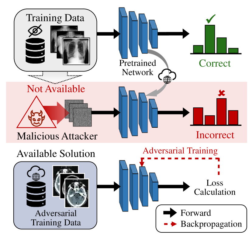
Unfortunately, the original training dataset is often not available in many real-world scenarios (Liu et al., 2021a; Hathaliya & Tanwar, 2020). While there are some public datasets available for certain domains (e.g., image classification), many real-world data are publicly unavailable due to privacy, security, or proprietary issues, with only the pretrained models available (Patashnik et al., 2021; Saharia et al., 2022; Ramesh et al., 2021). The problem becomes even more severe when it comes to specific domains that are privacy-sensitive (e.g., biometric, medical, etc.) where alternative datasets for training are difficult to find in the public. Therefore, if a user wants a pretrained model to become robust against adversarial attacks, there is currently no clear method to do so without the original training data.
In such circumstances, we study the problem of adversarial robustness under a more realistic and practical setting of data-free adversarial robustness, where a non-robustly pretrained model is given and its robust version should be learned without access to the original training data. To address the problem, we propose DataFreeShield, a novel method thoroughly designed to achieve robustness without any real data. Specifically, we propose a synthetic sample diversification method with dynamic synthetic loss modulation to maximize the diversity of the synthetic dataset. Moreover, we propose a gradient refinement method GradRefine to obtain a smoother loss surface, to minimize the impact of the distribution gap between synthetic and real data. Along with a soft guided training loss designed to maximize the transferability of robustness, DataFreeShield achieves significantly better robustness over prior art. To the best of our knowledge, this is the first work to faithfully address the definition of data-free adversarial robustness, and suggest an effective solution without relying on any real data.
Overall, our contributions are summarized as follows:
-
•
For the first time, we properly address the robustness problem in an entirely data-free manner, which gives adversarial robustness to non-robustly pretrained models without the original datasets.
-
•
To tackle the challenge of limited diversity in synthetic datasets, we devise diversified sample synthesis, a novel technique for generating synthetic samples.
-
•
We propose a gradient refinement method with a soft-guidance based training loss to minimize the impact of distribution shift incurred from synthetic data training.
-
•
We propose DataFreeShield, a completely data-free approach that can effectively convert a pretrained model to an adversarially robust one and show that DataFreeShield achieves significantly better robustness on various datasets over the baselines.
2 Background
2.1 Adversarial Robustness
Among many defense techniques for making DNN models robust against adversarial attacks, adversarial training (Madry et al., 2018) (AT) has been the most successful method, formulated as:
| (1) |
where is the loss function for classification (e.g., cross-entropy), is the number of training samples, and is the maximum perturbation limit. is an arbitrary adversarial sample that is generated based on to deceive the original decision, where is a popular choice. In practice, finding the optimal solution for the inner maximization is intractable, such that known adversarial attack methods are often used. For example, PGD (Madry et al., 2018) is a widely-used method, such that
| (2) |
where is the number of iteration steps. For each step, the image is updated to maximize the target loss, then projected onto the epsilon ball, denoted by .
2.2 Similar Approaches to Data-Free Robustness
One related approach to data-free robustness is test-time defense techniques (Nayak et al., 2022; Nie et al., 2022; Pérez et al., 2021) that do not train the target model but use separate modules for attack detection or purification. However, we find that those methods often rely on the availability of other data, or have limited applicability when used on their own. For instance, DAD (Nayak et al., 2022) uses the test set data for calibration, which could be regarded as a data leak. DiffPure (Nie et al., 2022) relies on diffusion models that are pretrained on a superset of the target dataset domain, restricting its use against unseen domains. TTE (Pérez et al., 2021) provides defense from augmentations agnostic to datasets. However, it is mainly used to enhance defense on models already adversarially trained, and its effect on non-robust models is marginal. Thus existing methods do not truthfully address the problem of data-free adversarial robustness, leaving vulnerability in data-absent situations.
2.3 Dataset Generation for Data-free Learning
When a model needs to be trained without the training data (i.e., data-free learning), a dominant approach is to generate a surrogate dataset, commonly adopted in data-free adaptations of knowledge distillation (Lopes et al., 2017; Fang et al., 2019), quantization (Xu et al., 2020; Choi et al., 2021), model extraction (Truong et al., 2021), or domain adaptation (Kurmi et al., 2021). Given only a pretrained model, the common choice for synthesis loss in the literature (Wang et al., 2021; Yin et al., 2020) are as follows:
| (3) | ||||
| (4) | ||||
| (5) |
where is the cross-entropy loss with artificial label among classes with the output of the model , regularizes the samples’ layer-wise distributions (, ) to follow the saved statistics in the batch normalization (,) over layers, and penalizes the total variance of the samples in pixel level. These losses are jointly used to train a generator (Liu et al., 2021c; Xu et al., 2020; Choi et al., 2021) or to directly optimize samples from noise (Wang et al., 2021; Yin et al., 2020; Ghiasi et al., 2022), with fixed hyperparameters :
| (6) |
3 Data-free Adversarial Robustness Problem
3.1 Problem Definition
In the problem of learning data-free adversarial robustness, the objective is to obtain a robust model from a pretrained original model , without access to its original training data . Hereafter, we will denote and as teacher and student, respectively.
In the problem, the typical AT formulation of Equation 1 cannot be directly applied because none of or is available for training or fine-tuning. Instead, following the common choice of data-free learning (Xu et al., 2020; Choi et al., 2022; Lopes et al., 2017), we choose to use a surrogate training dataset to train , which allows us to use the de facto standard method for adversarial robustness: adversarial training. With the given notations, we can reformulate the objective in Equation 1 as:
| (7) |
However, it remains to be answered how to create good surrogate training samples , and what loss function can best generalize the learned robustness to defend against attacks on real data.
3.2 Motivational Study
Here, we demonstrate the difficulty of the problem by answering one naturally arising question: Can we just use another real dataset? A relevant prior art is test-time defense such as DiffPure (Nie et al., 2022), or DAD (Nayak et al., 2022) which uses auxiliary models trained on large datasets (e.g., ImageNet) to improve defense on CIFAR-10. However, they strongly rely on the datasets from the same domain. In practice, there is no guarantee on such similarity, especially on tasks with specific domains (e.g., biomedical).
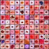
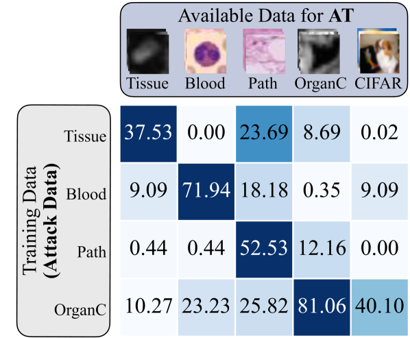
Figure 1(a) denotes the overall design of the motivational experiment, using biomedical image datasets from Yang et al. (2023). Assuming the absence of the dataset used for pretraining a given model, we use another dataset in the collection for additional adversarial training steps (Madry et al., 2018). Due to the different label spaces, we use teacher outputs as soft labels (i.e., ). Figure 1(b) shows the PGD-10 (, ) evaluation results using ResNet-18. Each row represents the dataset used for (non-robustly) pretraining a model, and each column represents the dataset used for additional adversarial training steps.
It is clear that models adversarially trained using alternative datasets show poor robustness compared to those trained using the original dataset (the diagonal cells). Although there exist a few combinations that obtain minor robustness from other datasets (e.g., Path → Tissue), they still suffer from large degradation compared to that of AT using the original dataset. Moreover, using a publicly available general domain dataset (CIFAR-10) also performs poorly, indicating that adversarial robustness is difficult to obtain from other datasets without access to the data in the same domain.
4 DataFreeShield: Learning Data-free Adversarial Robustness
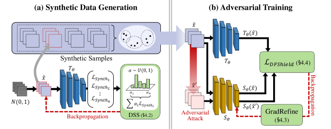
To tackle the data-free adversarial robustness problem, we propose DataFreeShield, an effective solution to improve the robustness of the target model without any real data. First, we generate a synthetic surrogate dataset using the information of the pretrained model (Figure 2(a)). Then, we use the synthetic dataset to adversarially train initialized with (Figure 2(b)). For generation, we propose diversified sample synthesis for dataset diversity (§4.2). For training, we propose a gradient refinement (§4.3) method and a soft-label guided objective function (§4.4).
4.1 Key Challenges
Although AT using a synthetic dataset seems like a promising approach, naively conducting the plan yields poor performance. We identify the following challenges to achieve high adversarial robustness.
Challenge 1: Limited Diversity of Synthetic Samples. Robust training of DNNs is known to require higher sample complexity (Khim & Loh, 2018; Yin et al., 2019) and substantially more data (Schmidt et al., 2018) than standard training. Recent findings (Rebuffi et al., 2021; Li & Spratling, 2022) appoint diversity as the key contributing factor to adversarial robustness, and (Sehwag et al., 2021) showed that enlarging train set is helpful only if it adds to the diversity of the data. Unfortunately, diversity is particularly hard to achieve in data-free methods, as they do not have direct access to training data distributions. While there exists a few data-free diversification techniques (Choi et al., 2021; Zhong et al., 2022; Han et al., 2021), they show negligible improvement in diversity, and often come at the price of low fidelity and quality. More importantly, none of these works contribute to enhancing adversarial robustness (See Table 7).
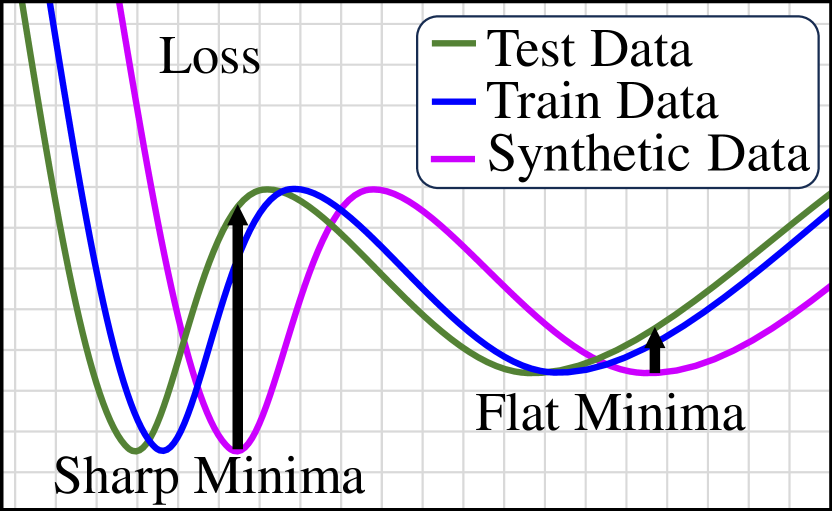
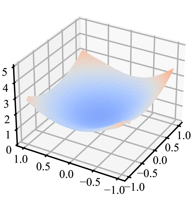
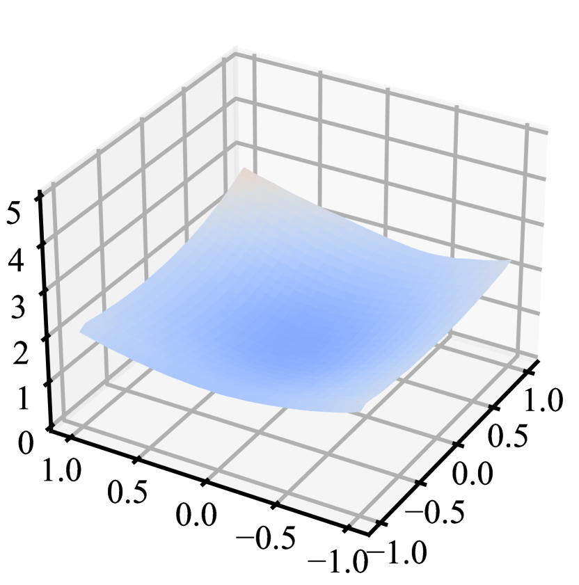
Challenge 2: Poor Generalization to Real Adversarial Samples. The ultimate goal of AT is to learn robustness that can be generalized to unseen adversaries. However, AT is known to be highly prone to robust overfitting (Rice et al., 2020; Stutz et al., 2021; Wu et al., 2020; Liu et al., 2020), where the model often fails to generalize the learned robustness to unseen data. Unfortunately, such difficulty is more severe in our problem. While the conventional overfitting problem is caused by the distributional gap between the training and test data, synthetic data will undergo a more drastic shift from the training data, further widening the gap. As illustrated in Figure 4(a), this double gap causes a large degradation in the test robustness. Many data-free learning methods study this distributional gap between synthetic and real data (Yin et al., 2020; Li et al., 2022; Choi et al., 2022), but none of them have addressed the problem under the light of adversarial robustness.
4.2 Diversified Sample Synthesis
To address the first key challenge of generating diverse samples, we propose a novel diversifying technique called diversified sample synthesis (DSS). We choose to directly optimize each sample one by one from a normal distribution through backpropagation using an objective function () (Yin et al., 2020; Cai et al., 2020; Zhong et al., 2022). In DSS, we leverage its characteristic to enhance the diversity of the samples, where we dynamically modulate the synthesis loss . We first formulate as a weighted sum of multiple losses. Then the weights are randomly set for every batch, giving each batch a distinct distribution. Given a set , the conventional approaches use their weighted sum with fixed hyperparameters as in Equation 6. On the other hand, we use coefficients differently sampled for every batch from a continuous space:
| (8) |
For the set , we use the three terms from Equation 6. The sampling of coefficients can follow any arbitrary distribution, where we choose a uniform distribution.
w/o GradRefine
w/ GradRefine
w/o GradRefine
w/ GradRefine
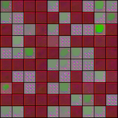
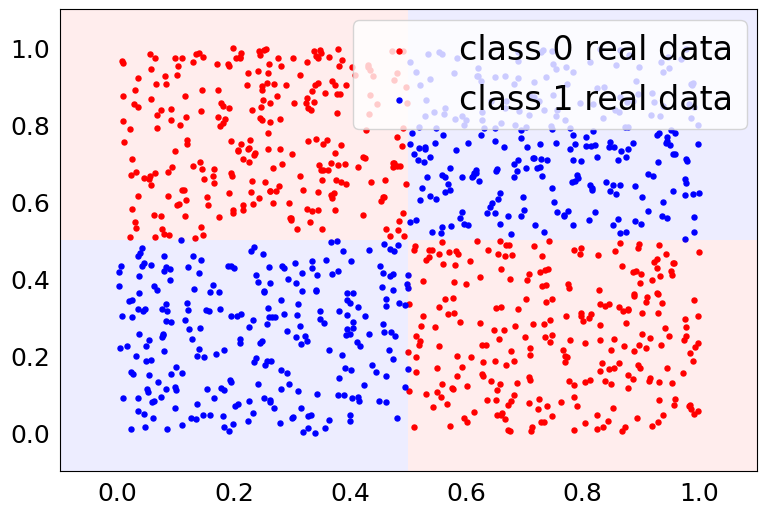
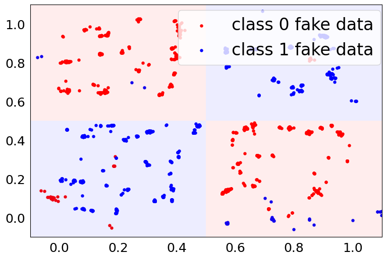
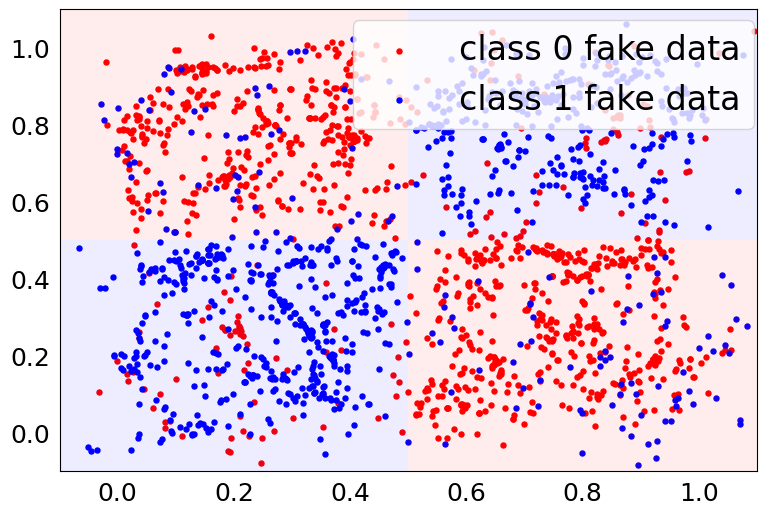
A Toy Experiment. To demonstrate the effectiveness DSS has on sample diversity, we conducted an empirical study on a toy experiment. Figure 3 displays the simplified experiment using 2-d data. The real data distribution is depicted in Figure 3(a). Using the real data, we train a 4-layer network with batch normalization. Figure 3(b) demonstrates the results from conventional approaches (fixed coefficients following (Yin et al., 2020)). Although the data generally follows class information, they are highly clustered with small variance. On the other hand, Figure 3(c) shows the data generated using DSS, which are highly diverse and exhibit coverage much closer to that of the real data distribution. In addition, we observe noisy samples in both Figure 3(b) and Figure 3(c). This is due to the nature of the synthetic data generation process, which uses artificial labels to guide synthetic samples towards given arbitrary classes. As these noisy samples may harm the training, we address this problem in Section 4.4.
4.3 Gradient Refinement for Smoother Loss Surface
As discussed in Section 4.1, the large distributional gap between synthetic and test data causes performance degradation. In such a case, searching for a flatter minima is a better strategy than searching for a low, but sharp minima as illustrated in Figure 4(a). For this, we devise a novel gradient refinement technique GradRefine. Inspired by a few techniques from domain generalization and federated learning (Tenison et al., 2022; Mansilla et al., 2021), GradRefine regularizes the influence of rapidly changing gradients during training. After computing gradients from mini-batches, we calculate the agreement score for each parameter as:
| (9) |
Intuitively, denotes the amount which one sign dominates the other. is bounded by [-1,1], where means equal distribution in both signs (maximum disagreement), and means one sign completely dominates the other (maximum agreement). Using , we compute the final gradient that will be used for parameter update:
| (10) |
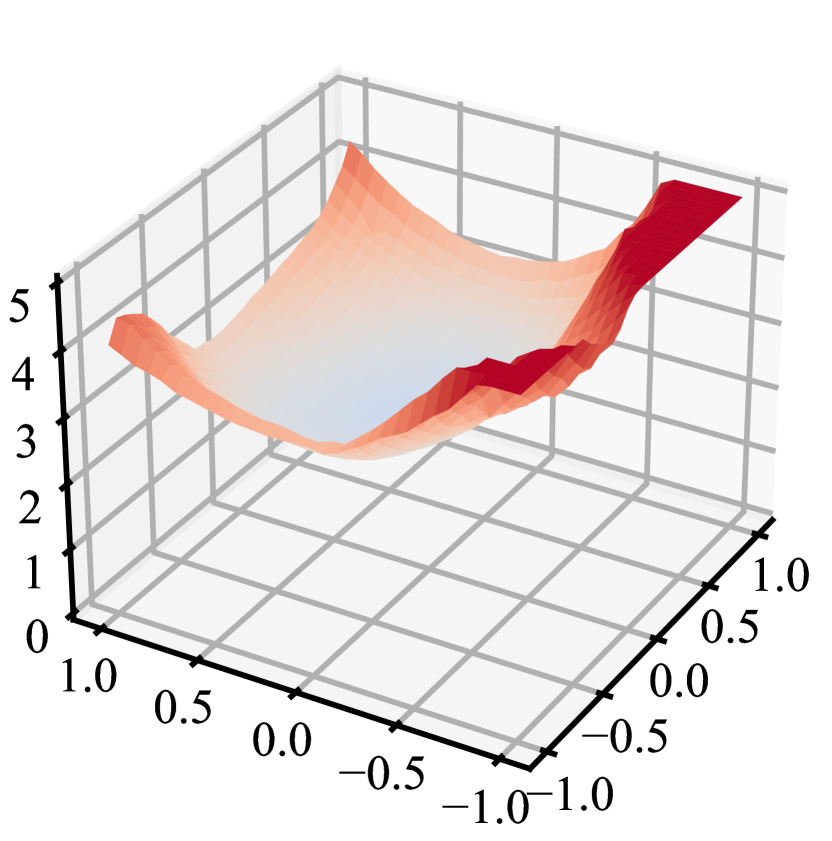
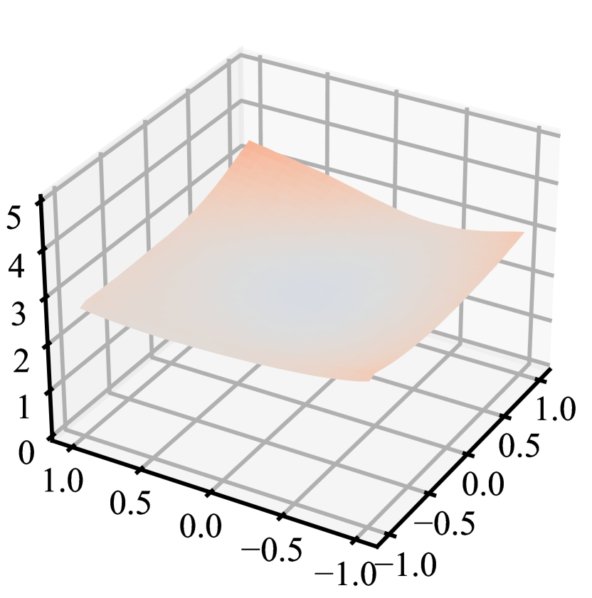
where is the indicator function, and is a masking function. We use value of 0.5, which indicates that one should dominate the other for more than half its entirety. This allows high-fluctuating parameters to be ignored by , and we further pursue alignment via selective use of agreeing gradient elements. Figure 4 (b)-(e) visualizes the effect of GradRefine on the loss surface. In both TRADES (Zhang et al., 2019) and (§4.4), GradRefine yields a flatter loss surface, contributing towards better performance. Please refer to Appendix H for the full set of visualization.
| Model | Method | Tissue | Blood | Path | OrganC | ||||||||
| RN-18 | Public | 22.04 | 00.02 | 00.00 | 09.09† | 09.09 | 00.00 | 13.30† | 00.00 | 00.00 | 79.41 | 40.10 | 36.53 |
| DaST | 23.27 | 07.01 | 05.98 | 16.92 | 06.75 | 04.82 | 07.49 | 03.36 | 01.20 | 83.13 | 27.91 | 24.49 | |
| DFME | 07.01 | 04.33 | 04.17 | 46.59 | 00.20 | 00.03 | 76.43 | 00.50 | 00.38 | 79.73 | 19.27 | 17.19 | |
| AIT | 15.62 | 11.64 | 09.72 | 18.24 | 10.55 | 01.64 | 16.66 | 10.24 | 03.89 | 56.85 | 18.02 | 16.67 | |
| DFARD | 09.31 | 08.48 | 01.87 | 22.60 | 10.17 | 09.70 | 11.59 | 04.93 | 03.18 | 81.97 | 21.71 | 19.50 | |
| Ours | 32.07 | 31.63 | 31.57 | 59.89 | 21.72 | 19.29 | 33.06 | 29.78 | 25.38 | 83.35 | 47.01 | 42.56 | |
| RN-50 | Public | 27.84 | 10.11 | 08.64 | 09.09† | 09.09 | 00.00 | 07.54 | 01.21 | 00.37 | 84.41 | 46.12 | 43.44 |
| DaST | 04.73 | 01.36 | 00.05 | 09.12 | 08.77 | 08.16 | 08.25 | 06.92 | 02.12 | 21.03 | 09.18 | 08.36 | |
| DFME | 07.13 | 06.55 | 04.76 | 07.16 | 03.36 | 03.19 | 80.10 | 02.28 | 02.01 | 27.76 | 22.00 | 21.78 | |
| AIT | 32.08 | 04.75 | 00.74 | 19.47 | 12.48 | 09.94 | 14.29 | 10.00 | 02.21 | 15.34 | 08.90 | 06.02 | |
| DFARD | 23.69 | 12.99 | 07.01 | 26.63 | 09.21 | 00.00 | 14.04 | 02.44 | 00.77 | 80.99 | 11.93 | 08.13 | |
| Ours | 31.91 | 27.15 | 26.68 | 74.63 | 36.07 | 30.17 | 41.63 | 15.35 | 12.28 | 86.56 | 62.60 | 59.86 | |
| †Did not converge | |||||||||||||
4.4 Training Objective Function
There exist several objective functions for adversarial training (Zhang et al., 2019; Wang et al., 2019; Goldblum et al., 2020; Zi et al., 2021). However, those objective functions mostly rely on the hard label of the dataset. For synthetic data, the assigned artificial labels are not ground truths, but simply target for optimization using cross-entropy loss. In such circumstances, relying on these artificial labels could convey incorrect guidance. As such, we devise a new objective function that does not rely on the hard label, but only utilizes the soft guidance from using KL-divergence.
| (11) |
The first term (a) optimizes the accuracy on clean samples, and can be thought as a replacement for the common cross-entropy loss. The second term (b) serves the purpose of learning adversarial robustness similar to the cross-entropy loss in standard AT (Equation 1). Adversarial samples exist because classifiers tend to rapidly change their decisions (Yang et al., 2020), due to failing to learn general features and instead relying on trivial features. To mitigate this, we add a smoothness term (c) which penalizes rapid changes in the model’s output. This regularizes the model’s sensitivity to small variations in the input, helping to train the target model to be stable under small perturbations.
| Baselines | ||
| DaST | ||
| DFME | ||
| AIT | ||
| DFARD |
5 Evaluation
5.1 Experimental Setup
We use total of four datasets: MedMNIST-v2 as medical datasets (Yang et al., 2023), SVHN (Netzer et al., 2011), CIFAR-10, and CIFAR-100 (Krizhevsky et al., 2009). For medical datasets, we use ResNet-18 and ResNet-50 as pretrained networks, and for perturbation budget. For CIFAR and SVHN datasets, we chose three pretrained models from PyTorchCV (pyt, ) library: ResNet-20, ResNet-56 (He et al., 2016), and WRN-28-10 (Zagoruyko & Komodakis, 2016). We use perturbation budget for SVHN, CIFAR-10, and CIFAR-100, and additionally examine setting. For results on extensive perturbation settings, please refer to Appendix E. For evaluation, AutoAttack (Croce & Hein, 2020) accuracy (denoted ) is generally perceived as the standard metric (Croce et al., 2020). While we regard as the primary interest, we also report the clean accuracy () and PGD-10 accuracy () for interested readers. Further details of experimental settings can be found in Appendix A.
5.2 Baselines
Since our work tackles a less-studied problem of data-free adversarial robustness with no known clear solution, it is important to set an adequate baseline for comparison. We choose four of the most relevant works of other data-free learning tasks that generate synthetic samples to replace the original: DaST (Zhou et al., 2020) from a black-box attack method, DFME (Truong et al., 2021) from data-free model extraction, AIT (Choi et al., 2022) from data-free quantization, and DFARD (Wang et al., 2023b) from data-free robust distillation. Since these four methods are not designed specifically for the data-free adversarial robustness problem, we adapt the training objective, summarized in Table 2. We also compare our method against test-time defense methods, including DAD (Nayak et al., 2022), TTE (Pérez et al., 2021), and DiffPure (Nie et al., 2022) on medical datasets. For details on the implementations, please refer to the experimental settings in Section A.4.
| ResNet-18 | ResNet-50 | ||||||
| Dataset | Method | ||||||
| Tissue | DAD | 55.86 | 22.90 | 04.38 | 59.72 | 31.59 | 03.49 |
| DiffPure | 26.17 | 22.85 | 09.06 | 27.73 | 27.54 | 01.81 | |
| TTE | 56.60 | 00.00 | 00.00 | 62.01 | 00.00 | 00.00 | |
| Ours | 32.07 | 31.63 | 31.57 | 31.91 | 27.15 | 26.68 | |
| Blood | DAD | 91.96 | 17.25 | 00.00 | 83.46 | 34.43 | 00.00 |
| DiffPure | 49.02 | 29.10 | 08.71 | 51.17 | 36.91 | 13.77 | |
| TTE | 09.09† | 09.09 | 08.92 | 16.84 | 00.03 | 00.00 | |
| Ours | 59.89 | 21.72 | 19.29 | 74.63 | 36.07 | 30.17 | |
| Path | DAD | 91.28 | 15.54 | 00.21 | 81.50 | 12.79 | 01.38 |
| DiffPure | 19.73 | 18.95 | 08.91 | 14.65 | 14.26 | 13.79 | |
| TTE | 76.56 | 00.64 | 00.36 | 75.08 | 04.23 | 01.88 | |
| Ours | 33.06 | 29.78 | 25.38 | 41.63 | 15.35 | 12.28 | |
| OrganC | DAD | 80.19 | 31.22 | 12.57 | 87.54 | 25.46 | 07.84 |
| DiffPure | 69.73 | 57.03 | 19.00 | 58.20 | 51.76 | 34.38 | |
| TTE | 61.03 | 22.90 | 15.98 | 56.54 | 25.82 | 18.63 | |
| Ours | 83.35 | 47.01 | 42.56 | 86.56 | 62.60 | 59.86 | |
| †Did not converge | |||||||
5.3 Performance Comparison
Privacy Sensitive Dataset. Table 1 shows experimental results for medical datasets, compared against the baseline methods (§5.2). The experiments represent a scenario close to real life where classification models are used for specific domains in the absence of public datasets from the same/similar domains. In all cases, DataFreeShield achieves the best results under evaluation. The baselines often perform worse than simply using public datasets of different domains. For example, in OrganC, using CIFAR-10 leads to some meaningful robustness. This could be because those datasets share similar features with CIFAR-10. Nonetheless, DataFreeShield performs significantly better in all cases.
We also show the limited applicability of existing test-time defense techniques in Table 3. Although they work relatively well on general domain data, they perform poorly on privacy-sensitive datasets with a large distributional gap to general ones. For example, DiffPure, which is known to show superior performance to AT methods, fails to show practical performance in most cases. Similarly, DAD performs poorly against AutoAttack, and TTE shows close-to-zero robustness in ResNet-50 in most settings.
General Domain Datasets. In Table 4, the performance of DataFreeShield is compared against the baselines on more general domain datasets: SVHN, CIFAR-10, and CIFAR-100. DataFreeShield outperforms the baselines by a huge margin. The improvements reach up to 23.19%p in , revealing the effectiveness of DataFreeShield and that the result is not from gradient obfuscation (Croce & Hein, 2020). Aligned with previous findings (Schmidt et al., 2018; Huang et al., 2022), models with larger capacity (ResNet-20 → ResNet-56 → WRN-28-10) tend to have significantly better robust accuracy of up to 21.08%p difference under AutoAttack. However, the baselines were often unable to exploit the model capacity (e.g., 19.65% → 14.57% in ResNet-56 → WRN-28-10 with DaST on SVHN), we believe this is due to the limited diversity of their synthetic samples. A similar trend can be found from the experiments with perturbation budgets shown in Table 5, where we compare with the best-performing baseline AIT from Table 4. Extended results using different budgets are presented in Appendix E.
| ResNet-20 | ResNet-56 | WRN-28-10 | |||||||
| SVHN | |||||||||
| DaST | 20.66 | 13.90 | 07.06 | 10.55 | 00.25 | 00.00 | 20.15 | 19.17 | 14.57 |
| DFME | 11.32 | 02.59 | 00.84 | 20.20 | 19.22 | 04.27 | 06.94 | 05.31 | 00.28 |
| AIT | 91.45 | 37.87 | 24.74 | 86.65 | 45.45 | 38.96 | 83.89 | 40.45 | 33.06 |
| DFARD | 25.62 | 18.65 | 00.19 | 19.58 | 15.43 | 00.00 | 92.32 | 13.08 | 00.01 |
| Ours | 91.83 | 54.82 | 47.55 | 88.66 | 62.05 | 57.54 | 94.14 | 69.60 | 62.66 |
| CIFAR-10 | |||||||||
| DaST | 10.00† | 09.89 | 08.62 | 12.06 | 07.68 | 05.32 | 10.00† | 09.65 | 02.85 |
| DFME | 14.36 | 05.23 | 00.08 | 13.81 | 03.92 | 00.03 | 10.00† | 09.98 | 00.05 |
| AIT | 32.89 | 11.93 | 10.67 | 38.47 | 12.29 | 11.36 | 34.92 | 10.90 | 09.47 |
| DFARD | 12.28 | 05.33 | 00.00 | 10.84 | 08.93 | 00.00 | 09.82 | 12.01 | 00.02 |
| Ours | 74.79 | 29.29 | 22.65 | 81.30 | 35.55 | 30.51 | 86.74 | 51.13 | 43.73 |
| CIFAR-100 | |||||||||
| DaST | 01.01† | 00.99 | 00.95 | 01.13 | 00.72 | 00.34 | 01.39 | 00.66 | 00.18 |
| DFME | 01.86 | 00.53 | 00.24 | 24.16 | 00.98 | 00.25 | 66.30 | 00.67 | 00.00 |
| AIT | 07.92 | 02.51 | 01.39 | 09.68 | 02.97 | 02.04 | 22.21 | 03.11 | 01.28 |
| DFARD | 66.59 | 00.02 | 00.00 | 69.20 | 00.26 | 00.00 | 82.03 | 01.10 | 00.00 |
| Ours | 41.67 | 10.41 | 05.97 | 39.29 | 13.23 | 09.49 | 61.35 | 23.22 | 16.44 |
| †Did not converge | |||||||||
| ResNet-20 | ResNet-56 | WRN-28-10 | |||||||
| SVHN | |||||||||
| AIT | 92.34 | 40.19 | 26.63 | 86.83 | 36.44 | 28.31 | 82.56 | 20.17 | 11.59 |
| Ours | 92.15 | 51.86 | 42.67 | 89.06 | 58.98 | 53.45 | 94.20 | 66.28 | 56.94 |
| CIFAR-10 | |||||||||
| AIT | 24.49 | 07.85 | 02.68 | 47.98 | 12.69 | 00.49 | 57.85 | 13.78 | 10.66 |
| Ours | 74.27 | 31.68 | 25.46 | 83.33 | 38.15 | 32.34 | 88.54 | 50.53 | 42.09 |
| CIFAR-100 | |||||||||
| AIT | 35.63 | 00.33 | 00.01 | 42.89 | 01.05 | 00.19 | 31.84 | 00.79 | 00.00 |
| Ours | 43.57 | 12.11 | 07.60 | 43.28 | 15.42 | 11.32 | 64.34 | 24.92 | 17.14 |
| Method | CIFAR-10 Accuracy | Diversity Metric | |||||
| Recall | Coverage | NDB | JSD | ||||
| Qimera | 76.88 | 18.90 | 10.68 | 0.000 | 0.002 | 99 | 0.514 |
| RDSKD | 10.00† | 10.00 | 10.00 | 0.000 | 0.001 | 98 | 0.658 |
| IntraQ | 13.77 | 36.13 | 12.46 | 0.308 | 0.087 | 88 | 0.275 |
| 91.46 | 43.66 | 36.34 | 0.535 | 0.101 | 91 | 0.253 | |
| + Mixup | 90.61 | 48.16 | 36.43 | 0.641 | 0.084 | 94 | 0.322 |
| + Cutout | 92.59 | 39.84 | 34.39 | 0.535 | 0.034 | 95 | 0.443 |
| + CutMix | 91.90 | 42.79 | 34.79 | 0.845 | 0.084 | 93 | 0.328 |
| + DSS | 88.16 | 50.13 | 41.40 | 0.830 | 0.163 | 88 | 0.211 |
| †Did not converge | |||||||
5.4 In-depth Study on DataFreeShield
We perform an in-depth study on DataFreeShield, and analyze the efficacy of each component. WRN-28-10 is mainly used, and more experiments can be found in the Appendix.
| SVHN | CIFAR-10 | |||||
| STD | 93.71 | 69.32 | 62.58 | 81.63 | 48.03 | 38.94 |
| TRADES | 94.12 | 69.10 | 61.75 | 79.61 | 45.86 | 37.08 |
| MART | 35.94 | 02.55 | 01.09 | 13.69 | 06.74 | 00.09 |
| ARD | 96.29 | 61.11 | 52.56 | 90.95 | 36.61 | 31.16 |
| RSLAD | 96.03 | 64.59 | 57.04 | 90.25 | 39.30 | 31.16 |
| 94.87 | 69.67 | 65.66 | 88.16 | 50.13 | 41.40 | |
Dataset Diversification. Table 6 compares DSS with other existing methods for dataset diversification. On the one hand, we choose three data-free synthesis baselines for comparison: Qimera (Choi et al., 2021), IntraQ (Zhong et al., 2022), and RDSKD (Han et al., 2021). We additionally test three image augmentation methods, Mixup (Huang et al., 2020), Cutout (DeVries & Taylor, 2017), and CutMix (Yun et al., 2019) on top of direct sample optimization (Yin et al., 2020), and for training we used for all cases. In terms of robustness, it is clear that DSS outperforms all other diversification methods in terms of .
For further investigation, we measure several well-known diversity metrics often used in evaluating generative models: recall, coverage (Naeem et al., 2020), number of statistically-different bins (NDB) (Richardson & Weiss, 2018), and Jensen-Shannon divergence (JSD). In almost all metrics, DSS shows the highest diversity, explaining its performance benefits. Although CutMix (Yun et al., 2019) shows slightly better recall than DSS, the difference is negligible and the coverage metric is generally perceived as a more exact measure of distributional diversity (Naeem et al., 2020). Measures on other datasets and models are in Appendix F.
Training Loss. Table 7 compares our proposed train loss against state-of-the-art ones used in adversarial training. STD (Madry et al., 2018), TRADES (Zhang et al., 2019), and MART (Wang et al., 2019) are from general adversarial training literature, while ARD (Goldblum et al., 2020) and RSLAD (Zi et al., 2021) are from robust distillation methods. Diversified sample synthesis was used for all cases for fair comparison. Interestingly, MART provides almost no robustness in our problem. MART encourages learning from misclassified samples, which may lead the model to overfit on synthetic samples. On the other hand, achieves the best results under both PGD-10 and AutoAttack in both datasets. The trend is consistent across different datasets and models, which we include in Appendix F.
| Model | DSS | GradRefine | |||
| ResNet-20 | ✗ | ✗ | ✗ | 86.42 | 02.03 |
| ✓ | ✗ | ✗ | 82.58 | 14.61 (+12.58) | |
| ✓ | ✓ | ✗ | 77.83 | 19.09 (+17.06) | |
| ✓ | ✓ | ✓ | 74.79 | 22.65 (+20.62) | |
| ResNet-56 | ✗ | ✗ | ✗ | 78.22 | 24.34 |
| ✓ | ✗ | ✗ | 83.72 | 27.42 (+3.08) | |
| ✓ | ✓ | ✗ | 83.67 | 27.69 (+3.35) | |
| ✓ | ✓ | ✓ | 81.30 | 30.51 (+6.17) | |
| WRN-28-10 | ✗ | ✗ | ✗ | 80.29 | 37.96 |
| ✓ | ✗ | ✗ | 91.46 | 36.34 (-1.62) | |
| ✓ | ✓ | ✗ | 88.16 | 41.40 (+3.44) | |
| ✓ | ✓ | ✓ | 86.74 | 43.73 (+5.77) |
Ablation Study. Table 8 shows an ablation study of DataFreeShield. The baseline where none of our methods are applied denotes using the exact same set of synthesis loss functions without DSS, and adversarial training is done via TRADES. Across all models, there is a consistent gain on . Applying , seems to slightly degrade on WRN-28-10, but when combined with the other techniques, it results in better performance as shown in Table 7. This is due to effectively reducing the gap between relatively weaker and stronger attacks. GradRefine adds a similar improvement, resulting in 6.17%p to 20.62%p gain altogether under AutoAttack.
| Gradient-free | Adaptive | ||||||
| SVHN | Clean | GenAtt. | BDRY | SPSA | AA | Automated | |
| RN20 | 91.83 | 90.28 | 91.77 | 60.99 | 47.55 | 47.25 | 47.52 |
| RN56 | 88.66 | 87.05 | 88.60 | 67.65 | 57.54 | 57.28 | 57.54 |
| WRN28 | 94.14 | 93.44 | 91.77 | 70.01 | 62.66 | 62.97 | 62.75 |
| CIFAR-10 | Clean | GenAtt. | BDRY | SPSA | AA | Automated | |
| RN20 | 74.79 | 72.92 | 74.73 | 34.58 | 22.65 | 22.62 | 22.65 |
| RN56 | 81.30 | 79.10 | 81.27 | 43.65 | 30.51 | 30.48 | 30.50 |
| WRN28 | 86.74 | 85.15 | 86.66 | 55.12 | 43.73 | 43.66 | 43.72 |
| Single | Iterative Attack | Unbound | |||||
| SVHN | Clean | ||||||
| RN20 | 91.83 | 85.86 | 78.02 | 57.57 | 54.82 | 53.81 | 0.00 |
| RN56 | 88.66 | 83.69 | 77.99 | 64.01 | 62.05 | 61.06 | 0.00 |
| WRN28 | 94.14 | 90.74 | 85.77 | 71.37 | 69.60 | 68.76 | 0.00 |
| CIFAR-10 | Clean | ||||||
| RN20 | 74.79 | 63.34 | 52.38 | 31.05 | 29.29 | 28.62 | 0.00 |
| RN56 | 81.30 | 71.47 | 59.98 | 38.02 | 35.55 | 34.30 | 0.00 |
| WRN28 | 86.74 | 80.16 | 72.20 | 53.26 | 51.13 | 50.32 | 0.00 |
5.5 Obfuscated Gradients
Gradient obfuscation (Athalye et al., 2018) refers to a case where a model either intentionally or unintentionally masks the gradient path that is necessary for optimization-based attacks. While these models seem robust against optimization attacks, they are easily attacked by gradient-free methods, demonstrating a false sense of robustness. Thus we conduct a series of experiments to validate that models trained using DataFreeShield do not fall into such case.
First, we use 3 gradient-free attacks: GenAttack (Alzantot et al., 2019), Boundary attack (Brendel et al., 2018), SPSA (Uesato et al., 2018), and 2 adaptive attacks: (Liu et al., 2022) and Automated (Yao et al., 2021) for evaluation. In Table 9, gradient-free attacks all fail to show higher attack success rate than optimization-based attacks (PGD and AutoAttack), meaning our method does not leverage gradient masking to circumvent optimization-based attacks. Also, in adaptive attacks, both and Automated show less than 1% degradation to the AutoAttack accuracy. Such consistent robustness across stronger adaptive attacks ensures that the evaluated robustness of DataFreeShield is not overestimated.
To further eliminate the possibility of gradient obfuscation, we observe DataFreeShield under increasing number of PGD iterations, including an unbounded attack (), shown in Table 10. According to Athalye et al. (2018), common signs of obfuscated gradients include single-step attack performing better than iterative attacks, unbounded attacks not reaching 100% attack success rate, and black-box attacks performing better than white-box attacks. In Table 9 and Table 10, we observe that DataFreeShield does not fall into any of these cases. Rather, we observe that increasing the number of iterations leads to better attack performance, and unbounded attacks reach 100% success rate in all cases. Note that GenAttack and Boundary attack are black-box attacks and their performance do not exceed other white-box attacks.
6 Related Work
Adversarial Defense. Existing defense methods train robust models by finetuning with adversarially perturbed data. Popular approaches include designing loss functions as variants of STD (Madry et al., 2018), such as TRADES (Zhang et al., 2019) or MART (Wang et al., 2019). While there exists other techniques for achieving robustness such as random smoothing (Szegedy et al., 2016), adversarial purification (Nie et al., 2022), or distillation (Zi et al., 2021; Goldblum et al., 2020), adversarial training and its variants are shown to be effective in most cases. A recent trend is to enhance the performance of adverarial training by importing extra data from other datasets (Carmon et al., 2019; Rebuffi et al., 2021), or generated under the supervision of real data (Rebuffi et al., 2021; Sehwag et al., 2021). However, such rich datasets are not easy to obtain in practice, sometimes none available in our setting.
Data-free Learning. Training or fine-tuning an existing model in absence of data has been studied to some degree. However, most are related to, or confined to only compression tasks, some of which are knowledge distillation (Fang et al., 2019; Lopes et al., 2017), pruning (Srinivas & Babu, 2015), and quantization (Nagel et al., 2019; Cai et al., 2020; Xu et al., 2020; Liu et al., 2021c; Choi et al., 2021, 2022; Zhu et al., 2021). A concurrent work DFARD (Wang et al., 2023b) sets a similar but different problem where a robust model already exists, and the objective is to distill it to a lighter network. Without the existence of a robust model, the effectiveness of DFARD is significantly reduced.
Gradient Refining Techniques. Adjusting gradients is a popular approach for diverse objectives. Yu et al. (2020) directly projects gradients with opposing directionality to dominant task gradients before model update. Liu et al. (2021b) selectively uses gradients that can best aid the worst performing task, and Fernando et al. (2022) estimates unbiased approximations of gradients to ensure convergence. Eshratifar et al. (2018) also utilizes gradients to maximize generalization ability to unseen data. Similar to ours, Mansilla et al. (2021) and Tenison et al. (2022) update the model based on sign agreement of gradients across domains or clients. Shi et al. (2022), Wang et al. (2023a), and Dandi et al. (2022) maximize gradient inner product between different domains or loss terms. While being effective, none target adversarial robustness, especially in data-free settings.
Loss Surface Smoothness and Generalization. Smoothness of loss surface is often associated with the model’s generalization ability. Keskar et al. (2017), Jiang et al. (2019), and Izmailov et al. (2018) have shown correlation between smoothness and generalization, using quantitative measures such as eigenvalues of the loss curvature. Sharpness-aware minimization methods (Foret et al., 2020; Wang et al., 2023a) leverage this knowledge to reduce the train-test generalization gap by explicitly regularizing the sharpness of the loss surface. Other methods (Terjék, 2019; Qin et al., 2019; Moosavi-Dezfooli et al., 2019) also implicitly regularize the model towards smoother minima. Notably, in the field where the generalization gap is more severe (e.g. domain generalization or federated learning), methods penalize gradients that hinder the smoothness of the landscape (Zhao et al., 2022), or regularize the model to have flatter landscapes across different domains of the dataset (Cha et al., 2021; Caldarola et al., 2022; Phan et al., 2022).
7 Conclusion
In this work, we study the problem of learning data-free adversarial robustness under the absence of real data. We propose DataFreeShield, an effective method for instilling robustness to a given model using synthetic data. We approach the problem from perspectives of generating diverse synthetic datasets and training with flatter loss surfaces. Further, we propose a new training loss function most suitable for our problem, and provide analysis on its effectiveness. Experimental results show that DataFreeShield significantly outperforms baseline approaches, demonstrating that it successfully achieves robustness without the original datasets.
Acknowledgements
This work was supported by the National Research Foundation of Korea (NRF) grant funded by the Korea government (MSIT) (2022R1C1C1011307), and Institute of Information & communications Technology Planning & Evaluation (IITP) ( RS-2023-00256081, RS-2024-00347394, RS-2022-II220959 (10%), RS-2021-II211343 (10%, SNU AI), RS-2021-II212068 (10%, AI Innov. Hub)) grant funded by the Korea government (MSIT).
Impact Statement
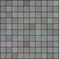
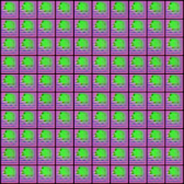
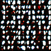
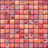
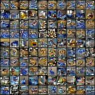
As shown in Appendix M, the generated samples are not very human-recognizable, and being so does not necessarily lead to better performance of the models. From these facts, we believe our synthetic input generation does not cause privacy invasion that might have existed from the original training dataset. However, there is still a possibility where the generated samples could affect privacy concerns, such as membership inference attacks (Shokri et al., 2017) or model stealing (Lee et al., 2019). For example, an attacker might compare the image-level or feature-level similarity of some test samples with the synthetically generated samples to find out whether the test sample is part of the training set or not. We believe further investigation is needed on such side-effects, which we leave as a future work.
References
- (1) Computer vision models on PyTorch. URL https://pypi.org/project/pytorchcv/.
- Alzantot et al. (2019) Alzantot, M., Sharma, Y., Chakraborty, S., Zhang, H., Hsieh, C.-J., and Srivastava, M. B. Genattack: Practical black-box attacks with gradient-free optimization. In Proceedings of the genetic and evolutionary computation conference, 2019.
- Athalye et al. (2018) Athalye, A., Carlini, N., and Wagner, D. Obfuscated gradients give a false sense of security: Circumventing defenses to adversarial examples. In International Conference on Machine Learning, 2018.
- Brendel et al. (2018) Brendel, W., Rauber, J., and Bethge, M. Decision-based adversarial attacks: Reliable attacks against black-box machine learning models. In Proceedings of International Conference on Learning Representations, 2018.
- Cai et al. (2020) Cai, Y., Yao, Z., Dong, Z., Gholami, A., Mahoney, M. W., and Keutzer, K. ZeroQ: A novel zero shot quantization framework. In Proceedings of the IEEE/CVF Conference on Computer Vision and Pattern Recognition, 2020.
- Caldarola et al. (2022) Caldarola, D., Caputo, B., and Ciccone, M. Improving generalization in federated learning by seeking flat minima. In European Conference on Computer Vision, 2022.
- Carmon et al. (2019) Carmon, Y., Raghunathan, A., Schmidt, L., Duchi, J. C., and Liang, P. S. Unlabeled data improves adversarial robustness. In Advances in Neural Information Processing Systems, 2019.
- Cha et al. (2021) Cha, J., Chun, S., Lee, K., Cho, H.-C., Park, S., Lee, Y., and Park, S. Swad: Domain generalization by seeking flat minima. Advances in Neural Information Processing Systems, 2021.
- Choi et al. (2021) Choi, K., Hong, D., Park, N., Kim, Y., and Lee, J. Qimera: Data-free quantization with synthetic boundary supporting samples. In Advances in Neural Information Processing Systems, 2021.
- Choi et al. (2022) Choi, K., Lee, H., Hong, D., Yu, J., Park, N., Kim, Y., and Lee, J. It’s all in the teacher: Zero-shot quantization brought closer to the teacher. In Proceedings of the IEEE/CVF Conference on Computer Vision and Pattern Recognition, 2022.
- Croce & Hein (2020) Croce, F. and Hein, M. Reliable evaluation of adversarial robustness with an ensemble of diverse parameter-free attacks. In International Conference on Machine Learning, 2020.
- Croce et al. (2020) Croce, F., Andriushchenko, M., Sehwag, V., Debenedetti, E., Flammarion, N., Chiang, M., Mittal, P., and Hein, M. Robustbench: a standardized adversarial robustness benchmark. arXiv preprint arXiv:2010.09670, 2020.
- Dandi et al. (2022) Dandi, Y., Barba, L., and Jaggi, M. Implicit gradient alignment in distributed and federated learning. In Proceedings of the AAAI Conference on Artificial Intelligence, 2022.
- DeVries & Taylor (2017) DeVries, T. and Taylor, G. W. Improved regularization of convolutional neural networks with cutout. arXiv preprint arXiv:1708.04552, 2017.
- Eshratifar et al. (2018) Eshratifar, A. E., Eigen, D., and Pedram, M. Gradient agreement as an optimization objective for meta-learning. arXiv preprint arXiv:1810.08178, 2018.
- Fang et al. (2019) Fang, G., Song, J., Shen, C., Wang, X., Chen, D., and Song, M. Data-free adversarial distillation. arXiv preprint arXiv:1912.11006, 2019.
- Fernando et al. (2022) Fernando, H. D., Shen, H., Liu, M., Chaudhury, S., Murugesan, K., and Chen, T. Mitigating gradient bias in multi-objective learning: A provably convergent approach. In International Conference on Learning Representations, 2022.
- Foret et al. (2020) Foret, P., Kleiner, A., Mobahi, H., and Neyshabur, B. Sharpness-aware minimization for efficiently improving generalization. In International Conference on Learning Representations, 2020.
- Ghiasi et al. (2022) Ghiasi, A., Kazemi, H., Reich, S., Zhu, C., Goldblum, M., and Goldstein, T. Plug-in inversion: Model-agnostic inversion for vision with data augmentations. In International Conference on Machine Learning, 2022.
- Goldblum et al. (2020) Goldblum, M., Fowl, L., Feizi, S., and Goldstein, T. Adversarially robust distillation. In Proceedings of the AAAI Conference on Artificial Intelligence, 2020.
- Goodfellow et al. (2014) Goodfellow, I., Pouget-Abadie, J., Mirza, M., Xu, B., Warde-Farley, D., Ozair, S., Courville, A., and Bengio, Y. Generative adversarial nets. In Advances in Neural Information Processing Systems, 2014.
- Goodfellow et al. (2015) Goodfellow, I. J., Shlens, J., and Szegedy, C. Explaining and harnessing adversarial examples. In International Conference on Learning Representations, 2015.
- Han et al. (2021) Han, P., Park, J., Wang, S., and Liu, Y. Robustness and diversity seeking data-free knowledge distillation. In IEEE International Conference on Acoustics, Speech and Signal Processing, 2021.
- Hathaliya & Tanwar (2020) Hathaliya, J. J. and Tanwar, S. An exhaustive survey on security and privacy issues in healthcare 4.0. Computer Communications, 2020.
- He et al. (2016) He, K., Zhang, X., Ren, S., and Sun, J. Deep residual learning for image recognition. In Proceedings of the IEEE/CVF Conference on Computer Vision and Pattern Recognition, 2016.
- Huang et al. (2020) Huang, L., Zhang, C., and Zhang, H. Self-adaptive training: Beyond empirical risk minimization. In Advances in Neural Information Processing Systems, 2020.
- Huang et al. (2022) Huang, S., Lu, Z., Deb, K., and Boddeti, V. N. Revisiting residual networks for adversarial robustness: An architectural perspective. arXiv preprint arXiv:2212.11005, 2022.
- Izmailov et al. (2018) Izmailov, P., Podoprikhin, D., Garipov, T., Vetrov, D., and Wilson, A. G. Averaging weights leads to wider optima and better generalization. In 34th Conference on Uncertainty in Artificial Intelligence, 2018.
- Jiang et al. (2019) Jiang, Y., Neyshabur, B., Mobahi, H., Krishnan, D., and Bengio, S. Fantastic generalization measures and where to find them. In International Conference on Learning Representations, 2019.
- Keskar et al. (2017) Keskar, N. S., Mudigere, D., Nocedal, J., Smelyanskiy, M., and Tang, P. T. P. On large-batch training for deep learning: Generalization gap and sharp minima. In International Conference on Learning Representations, 2017.
- Khim & Loh (2018) Khim, J. and Loh, P.-L. Adversarial risk bounds via function transformation. arXiv preprint arXiv:1810.09519, 2018.
- Krizhevsky et al. (2009) Krizhevsky, A., Hinton, G., et al. Learning multiple layers of features from tiny images, 2009. URL http://www.cs.utoronto.ca/~kriz/learning-features-2009-TR.pdf.
- Kurmi et al. (2021) Kurmi, V. K., Subramanian, V. K., and Namboodiri, V. P. Domain impression: A source data free domain adaptation method. In Proceedings of the IEEE/CVF winter conference on applications of computer vision, 2021.
- Lee et al. (2019) Lee, T., Edwards, B., Molloy, I., and Su, D. Defending against neural network model stealing attacks using deceptive perturbations. In IEEE Security and Privacy Workshops, 2019.
- Li et al. (2018) Li, H., Xu, Z., Taylor, G., Studer, C., and Goldstein, T. Visualizing the loss landscape of neural nets. In Advances in Neural Information Processing Systems, 2018.
- Li & Spratling (2022) Li, L. and Spratling, M. W. Data augmentation alone can improve adversarial training. In The International Conference on Learning Representations, 2022.
- Li et al. (2022) Li, Z., Ma, L., Chen, M., Xiao, J., and Gu, Q. Patch similarity aware data-free quantization for vision transformers. In European Conference on Computer Vision, 2022.
- Liu et al. (2021a) Liu, B., Ding, M., Shaham, S., Rahayu, W., Farokhi, F., and Lin, Z. When machine learning meets privacy: A survey and outlook. ACM Computing Surveys, 2021a.
- Liu et al. (2021b) Liu, B., Liu, X., Jin, X., Stone, P., and Liu, Q. Conflict-averse gradient descent for multi-task learning. In Advances in Neural Information Processing Systems, 2021b.
- Liu et al. (2020) Liu, C., Salzmann, M., Lin, T., Tomioka, R., and Süsstrunk, S. On the loss landscape of adversarial training: Identifying challenges and how to overcome them. In Advances in Neural Information Processing Systems, 2020.
- Liu et al. (2021c) Liu, Y., Zhang, W., and Wang, J. Zero-shot adversarial quantization. In Proceedings of the IEEE/CVF Conference on Computer Vision and Pattern Recognition, 2021c.
- Liu et al. (2022) Liu, Y., Cheng, Y., Gao, L., Liu, X., Zhang, Q., and Song, J. Practical evaluation of adversarial robustness via adaptive auto attack. In Proceedings of the IEEE/CVF Conference on Computer Vision and Pattern Recognition, 2022.
- Lopes et al. (2017) Lopes, R. G., Fenu, S., and Starner, T. Data-free knowledge distillation for deep neural networks. In Advances in Neural Information Processing Systems Workshops, 2017.
- Madry et al. (2018) Madry, A., Makelov, A., Schmidt, L., Tsipras, D., and Vladu, A. Towards deep learning models resistant to adversarial attacks. In International Conference on Learning Representations, 2018.
- Mansilla et al. (2021) Mansilla, L., Echeveste, R., Milone, D. H., and Ferrante, E. Domain generalization via gradient surgery. In Proceedings of the IEEE/CVF International Conference on Computer Vision, 2021.
- Moosavi-Dezfooli et al. (2019) Moosavi-Dezfooli, S.-M., Fawzi, A., Uesato, J., and Frossard, P. Robustness via curvature regularization, and vice versa. In Proceedings of the IEEE/CVF Conference on Computer Vision and Pattern Recognition, 2019.
- Naeem et al. (2020) Naeem, M. F., Oh, S. J., Uh, Y., Choi, Y., and Yoo, J. Reliable fidelity and diversity metrics for generative models. In International Conference on Machine Learning, 2020.
- Nagel et al. (2019) Nagel, M., Baalen, M. v., Blankevoort, T., and Welling, M. Data-free quantization through weight equalization and bias correction. In Proceedings of the IEEE International Conference on Computer Vision, 2019.
- Nayak et al. (2022) Nayak, G. K., Rawal, R., and Chakraborty, A. Dad: Data-free adversarial defense at test time. In Proceedings of the IEEE/CVF Winter Conference on Applications of Computer Vision, 2022.
- Netzer et al. (2011) Netzer, Y., Wang, T., Coates, A., Bissacco, A., Wu, B., and Ng, A. Y. Reading digits in natural images with unsupervised feature learning. In Advances in Neural Information Processing Systems Workshops, 2011.
- Nie et al. (2022) Nie, W., Guo, B., Huang, Y., Xiao, C., Vahdat, A., and Anandkumar, A. Diffusion models for adversarial purification. In International Conference on Machine Learning, 2022.
- Odena et al. (2017) Odena, A., Olah, C., and Shlens, J. Conditional image synthesis with auxiliary classifier GANs. In International Conference on Machine Learning, 2017.
- Patashnik et al. (2021) Patashnik, O., Wu, Z., Shechtman, E., Cohen-Or, D., and Lischinski, D. Styleclip: Text-driven manipulation of stylegan imagery. In Proceedings of the IEEE International Conference on Computer Vision, 2021.
- Pérez et al. (2021) Pérez, J. C., Alfarra, M., Jeanneret, G., Rueda, L., Thabet, A., Ghanem, B., and Arbeláez, P. Enhancing adversarial robustness via test-time transformation ensembling. In Proceedings of International Conference on Computer Vision, 2021.
- Phan et al. (2022) Phan, H., Tran, L., Tran, N. N., Ho, N., Phung, D., and Le, T. Improving multi-task learning via seeking task-based flat regions. arXiv preprint arXiv:2211.13723, 2022.
- Qin et al. (2019) Qin, C., Martens, J., Gowal, S., Krishnan, D., Dvijotham, K., Fawzi, A., De, S., Stanforth, R., and Kohli, P. Adversarial robustness through local linearization. Advances in Neural Information Processing Systems, 2019.
- Ramesh et al. (2021) Ramesh, A., Pavlov, M., Goh, G., Gray, S., Voss, C., Radford, A., Chen, M., and Sutskever, I. Zero-shot text-to-image generation. In International Conference on Machine Learning, 2021.
- Rebuffi et al. (2021) Rebuffi, S.-A., Gowal, S., Calian, D. A., Stimberg, F., Wiles, O., and Mann, T. A. Data augmentation can improve robustness. In Advances in Neural Information Processing Systems, 2021.
- Rice et al. (2020) Rice, L., Wong, E., and Kolter, Z. Overfitting in adversarially robust deep learning. In Proceedings of the International Conference on Machine Learning, 2020.
- Richardson & Weiss (2018) Richardson, E. and Weiss, Y. On gans and gmms. In Advances in Neural Information Processing Systems, 2018.
- Sabour et al. (2016) Sabour, S., Cao, Y., Faghri, F., and Fleet, D. J. Adversarial manipulation of deep representations. International Conference on Learning Representations, 2016.
- Saharia et al. (2022) Saharia, C., Chan, W., Saxena, S., Li, L., Whang, J., Denton, E. L., Ghasemipour, K., Gontijo Lopes, R., Karagol Ayan, B., Salimans, T., et al. Photorealistic text-to-image diffusion models with deep language understanding. In Advances in Neural Information Processing Systems, 2022.
- Schmidt et al. (2018) Schmidt, L., Santurkar, S., Tsipras, D., Talwar, K., and Madry, A. Adversarially robust generalization requires more data. In Advances in Neural Information Processing Systems, 2018.
- Sehwag et al. (2021) Sehwag, V., Mahloujifar, S., Handina, T., Dai, S., Xiang, C., Chiang, M., and Mittal, P. Robust learning meets generative models: Can proxy distributions improve adversarial robustness? In International Conference on Learning Representations, 2021.
- Shi et al. (2022) Shi, Y., Seely, J., Torr, P., N, S., Hannun, A., Usunier, N., and Synnaeve, G. Gradient matching for domain generalization. In International Conference on Learning Representations, 2022.
- Shokri et al. (2017) Shokri, R., Stronati, M., Song, C., and Shmatikov, V. Membership inference attacks against machine learning models. In IEEE Symposium on Security and Privacy, 2017.
- Srinivas & Babu (2015) Srinivas, S. and Babu, R. V. Data-free parameter pruning for deep neural networks. In British Machine Vision Conference, 2015.
- Stutz et al. (2021) Stutz, D., Hein, M., and Schiele, B. Relating adversarially robust generalization to flat minima. In Proceedings of the IEEE/CVF International Conference on Computer Vision, 2021.
- Szegedy et al. (2014) Szegedy, C., Zaremba, W., Sutskever, I., Bruna, J., Erhan, D., Goodfellow, I., and Fergus, R. Intriguing properties of neural networks. In International Conference on Learning Representations, 2014.
- Szegedy et al. (2016) Szegedy, C., Vanhoucke, V., Ioffe, S., Shlens, J., and Wojna, Z. Rethinking the inception architecture for computer vision. In Proceedings of the IEEE/CVF Conference on Computer Vision and Pattern Recognition, 2016.
- Tenison et al. (2022) Tenison, I., Sreeramadas, S. A., Mugunthan, V., Oyallon, E., Belilovsky, E., and Rish, I. Gradient masked averaging for federated learning. arXiv preprint arXiv:2201.11986, 2022.
- Terjék (2019) Terjék, D. Adversarial lipschitz regularization. In International Conference on Learning Representations, 2019.
- Truong et al. (2021) Truong, J.-B., Maini, P., Walls, R. J., and Papernot, N. Data-free model extraction. In Proceedings of the IEEE/CVF Conference on Computer Vision and Pattern Recognition, 2021.
- Uesato et al. (2018) Uesato, J., O’donoghue, B., Kohli, P., and Oord, A. Adversarial risk and the dangers of evaluating against weak attacks. In Proceedings of International Conference on Machine Learning, 2018.
- Wang et al. (2021) Wang, P., Li, Y., Singh, K. K., Lu, J., and Vasconcelos, N. Imagine: Image synthesis by image-guided model inversion. In Proceedings of the IEEE/CVF Conference on Computer Vision and Pattern Recognition, 2021.
- Wang et al. (2023a) Wang, P., Zhang, Z., Lei, Z., and Zhang, L. Sharpness-aware gradient matching for domain generalization. In Proceedings of the IEEE/CVF Conference on Computer Vision and Pattern Recognition, 2023a.
- Wang et al. (2019) Wang, Y., Zou, D., Yi, J., Bailey, J., Ma, X., and Gu, Q. Improving adversarial robustness requires revisiting misclassified examples. In International Conference on Learning Representations, 2019.
- Wang et al. (2023b) Wang, Y., Chen, Z., Yang, D., Guo, P., Jiang, K., Zhang, W., and Qi, L. Model robustness meets data privacy: Adversarial robustness distillation without original data. arXiv preprint arXiv:2303.11611, 2023b.
- Wu et al. (2020) Wu, D., Xia, S.-T., and Wang, Y. Adversarial weight perturbation helps robust generalization. In Advances in Neural Information Processing Systems, 2020.
- Xu et al. (2020) Xu, S., Li, H., Zhuang, B., Liu, J., Cao, J., Liang, C., and Tan, M. Generative low-bitwidth data free quantization. In European Conference on Computer Vision, 2020.
- Yang et al. (2023) Yang, J., Shi, R., Wei, D., Liu, Z., Zhao, L., Ke, B., Pfister, H., and Ni, B. Medmnist v2-a large-scale lightweight benchmark for 2d and 3d biomedical image classification. Scientific Data, 2023.
- Yang et al. (2020) Yang, Y.-Y., Rashtchian, C., Zhang, H., Salakhutdinov, R. R., and Chaudhuri, K. A closer look at accuracy vs. robustness. Advances in Neural Information Processing Systems, 2020.
- Yao et al. (2021) Yao, C., Bielik, P., Tsankov, P., and Vechev, M. Automated discovery of adaptive attacks on adversarial defenses. Advances in Neural Information Processing Systems, 2021.
- Yin et al. (2019) Yin, D., Kannan, R., and Bartlett, P. Rademacher complexity for adversarially robust generalization. In International Conference on Machine Learning, 2019.
- Yin et al. (2020) Yin, H., Molchanov, P., Alvarez, J. M., Li, Z., Mallya, A., Hoiem, D., Jha, N. K., and Kautz, J. Dreaming to distill: Data-free knowledge transfer via deepinversion. In Proceedings of the IEEE/CVF Conference on Computer Vision and Pattern Recognition, 2020.
- Yu et al. (2020) Yu, T., Kumar, S., Gupta, A., Levine, S., Hausman, K., and Finn, C. Gradient surgery for multi-task learning. In Advances in Neural Information Processing Systems, 2020.
- Yun et al. (2019) Yun, S., Han, D., Oh, S. J., Chun, S., Choe, J., and Yoo, Y. Cutmix: Regularization strategy to train strong classifiers with localizable features. In Proceedings of the IEEE/CVF International Conference on Computer Vision, 2019.
- Zagoruyko & Komodakis (2016) Zagoruyko, S. and Komodakis, N. Wide residual networks. In British Machine Vision Conference, 2016.
- Zhang et al. (2019) Zhang, H., Yu, Y., Jiao, J., Xing, E., El Ghaoui, L., and Jordan, M. Theoretically principled trade-off between robustness and accuracy. In International Conference on Machine Learning, 2019.
- Zhao et al. (2022) Zhao, Y., Zhang, H., and Hu, X. Penalizing gradient norm for efficiently improving generalization in deep learning. In International Conference on Machine Learning, 2022.
- Zhong et al. (2022) Zhong, Y., Lin, M., Nan, G., Liu, J., Zhang, B., Tian, Y., and Ji, R. Intraq: Learning synthetic images with intra-class heterogeneity for zero-shot network quantization. In Proceedings of the IEEE/CVF Conference on Computer Vision and Pattern Recognition, 2022.
- Zhou et al. (2020) Zhou, M., Wu, J., Liu, Y., Liu, S., and Zhu, C. Dast: Data-free substitute training for adversarial attacks. In Proceedings of the IEEE/CVF Conference on Computer Vision and Pattern Recognition, 2020.
- Zhu et al. (2021) Zhu, B., Hofstee, P., Peltenburg, J., Lee, J., and Alars, Z. AutoReCon: Neural architecture search-based reconstruction for data-free compression. In International Joint Conferences on Artificial Intelligence, 2021.
- Zhu et al. (2022) Zhu, J., Yao, J., Han, B., Zhang, J., Liu, T., Niu, G., Zhou, J., Xu, J., and Yang, H. Reliable adversarial distillation with unreliable teachers. In International Conference on Learning Representations, 2022.
- Zi et al. (2021) Zi, B., Zhao, S., Ma, X., and Jiang, Y.-G. Revisiting adversarial robustness distillation: Robust soft labels make student better. In Proceedings of the IEEE International Conference on Computer Vision, 2021.
Appendix
We provide a more extensive set of experimental results with some analyses that we could not include in the main body due to space constraints. The contents of this material are as below:
-
•
Detailed Experimental Settings (Appendix A): We provide detailed information of our experiments.
-
•
Overall Procedure of DataFreeShield (Appendix B): We provide pseudo-code of the overall procedure of DataFreeShield.
-
•
Number of Synthetic Samples (Appendix C): We study the effect of using different numbers of synthetic samples.
-
•
Extended Set of Experiments on medical dataset (Appendix D): Extended results on medical dataset are reported.
-
•
Extended Set of Experiments on -bounds (Appendix E): Extended results on diverse attack distance are presented.
-
•
Detailed Study on DataFreeShield (Appendix F): Extended results of detailed study of DataFreeShield on sample diversity and comparison against different training loss functions.
-
•
Evaluation under Modified Attacks (Appendix G: We evaluate robustness of DataFreeShield under modified attacks.
-
•
Further Visualization of Loss Surface (Appendix H): We provide further analysis on and its effect on the loss surface.
-
•
Sensitivity Study on the Number of Aggregated Batches (Appendix I): We conduct sensitivity study on the number of aggregated batches.
-
•
Sensitivity Study on (Appendix J): We conduct sensitivity study on the threshold value used in GradRefine.
-
•
Sensitivity Study on and (Appendix K): We conduct sensitivity study on the hyperparameters of , and .
-
•
Visualization of DSS using PCA (Appendix L): We provide PCA visualizations of different synthetic datasets to study the effect of DSS on diversity.
-
•
Generated Synthetic Data (Appendix M): Selected examples of synthetic data are presented.
Appendix A Detailed Experimental Settings
In this section, we provide details on experimental settings for both synthetic data generation and robust training. For baseline implementation of DaST (Zhou et al., 2020), DFME (Truong et al., 2021), and AIT (Choi et al., 2022), we used the original code from the authors, except for the modifications we specified in Section A.4. For DFARD (Wang et al., 2023b) we followed the description in the publication since the original implementation is not available, and used ACGAN (Odena et al., 2017) due to missing details of a generator architecture in the original publication. All experiments have been conducted using PyTorch 1.9.1 and Python 3.8.0 running on Ubuntu 20.04.3 LTS with CUDA version 11.1 using RTX3090 and A6000 GPUs.
A.1 Code
The code used for the experiment is included in a zip archive in the supplementary material, along with the script for reproduction. The code is under Nvidia Source Code License-NC and GNU General Public License v3.0.
A.2 Data Generation
When optimizing gaussian noise, we use Adam optimizer with learning rate with batch size of 200, which we optimize for 1000 iterations on medical datasets and 2000 on general domain datasets. For diversified sample synthesis, we set the range [0,1] for the sampling distribution of coefficients, and use uniform distribution. Code implementation for diversified sample synthesis builds upon a prior work (Yin et al., 2020). For medical datasets results, we generated 10,000 samples for training, and for the other datasets we used 60,000 samples. To accelerate data generation, we use multiple GPUs in parallel where 10,000 samples are generated with each. With batch size of 200, generating 10,000 samples of size 2828 using ResNet-18 takes 0.7 hours on RTX 3090. For 3232 sized samples, ResNet-20 takes 0.6 hours, ResNet-56 2.6 hours, and WRN-28-10 3.6 hours.
For medical datasets, we trained two network architectures ResNet-18 and ResNet-50 used in the original paper (Yang et al., 2023). We report the pretraining results in Table 11.
| Dataset | ResNet-18 | ResNet-50 |
| Tissue | 67.62 | 68.29 |
| Blood | 95.53 | 95.00 |
| Derma | 74.61 | 73.92 |
| Path | 92.19 | 91.41 |
| OCT | 80.60 | 84.90 |
| OrganA | 93.75 | 94.04 |
| OrganC | 90.74 | 91.06 |
| OrganS | 78.75 | 78.37 |
A.3 Adversarial Training
For adversarial training, we used SGD optimizer with learning rate=1e-4, momentum=0.9, and batch size of 200 for 100 epochs, and 200 epochs for ResNet-20 and ResNet-18. All adversarial perturbations were created using PGD-10 (Madry et al., 2018) with the specified -bounds. Following the convention, -norm attacks are bounded by with step size of . -norm attacks are evaluated under a diverse set of distances , which all use step size. For , we simply use and , which we found to best balance the learning from three different objective terms. For GradRefine, we use for all settings, which we found to perform generally well across different datasets and models. When using GradRefine, we increment the learning rate linearly with to take into consideration the increased effective batch size. We use for all our experiments with GradRefine.
A.4 Adaptation of the Baselines
In this section, we describe how we adapted the baselines (Table 2) to the problem of data-free adversarial robustness. DaST (Zhou et al., 2020) is a black-box attack method with no access to the original data. DaST trains a substitute model using samples from a generative model (Goodfellow et al., 2014) to synthesize samples for querying the victim model. To adapt DaST to our problem, we keep the overall framework but modify the training loss, substituting clean samples with perturbed ones. This makes it possible to use the training algorithm, while the objective now is to robustly train a model with no data.
DFME (Truong et al., 2021) is a more recent work on data-free model extraction that also utilizes synthetic samples for model stealing. They leverage distillation methods (Fang et al., 2019) to synthesize samples that maximize student-teacher disagreement. Similar to DaST, we substitute the student input to perturbed ones, while keeping other settings the same.
AIT (Choi et al., 2022) utilizes the full precision model’s feedback for training its generative model. Unlike DaST and DFME which focus on student outputs when training the generator, AIT additionally utilizes the batch-normalization statistics stored in the teacher model for creating synthetic samples. Since AIT is a model quantization method, its student model is of low-bit precision, and thus their training loss cannot be directly adopted to our task. We use TRADES (Zhang et al., 2019) loss function for training, a variation of STD (Madry et al., 2018).
Lastly, DFARD (Wang et al., 2023b) suggests data-free robust distillation. Given a model already robustly trained, the goal is to distill its robustness to a lighter network. They use adaptive distillation temperature to regulate learning difficulty. While this seems to align with the data-free adversarial robustness, the robust teacher is not available in our problem. Therefore, we replace the robustly pretrained model with the given (non-robust) so that student can correctly classify perturbed samples.
For implementations of test-time defense techniques including DAD (Nayak et al., 2022), DiffPure (Nie et al., 2022), and TTE (Pérez et al., 2021), we used the official code provided by the authors. For DAD, we follow their method and retrain a CIFAR-10 pretrained detector on medical datasets test set. Since their method assumes the usability of off-the-shelf detector, we used their pretrained detector trained on CIFAR-10 and fine-tuned it using each dataset from medical datasets. Note that DAD is evaluated on the same test set that is used to finetune the detector module, which could be considered data leak. For TTE, where we used +flip+4crops+4 flipped-crops as it is reported as the best setting in the original paper. Lastly, for DiffPure, we used the same setting the authors used for evaluating on CIFAR-10 dataset, including the pretrained score SDE model. To match the image size of the pretrained model, we resized the image samples originally sized as 28x28 to 32x32. Also, note that DiffPure requires high computational cost for evaluating against adaptive attacks such as AutoAttack (Croce & Hein, 2020), and so the authors random sample 512 images for all evaluations. However, we used 2000 images randomly sampled from the test set for more accurate evaluation, except for the cases where the test set is smaller than 2000.
Appendix B Overall Procedure of DataFreeShield
The pseudo-code of the overall procedure of DataFreeShield is depicted in Algorithm 1. It comprises data generation using diversified sample synthesis (line 4-10, §4.2), and adversarial training using a novel loss function (line 15, §4.4) along with a gradient refinement technique (line 17-20, §4.3).
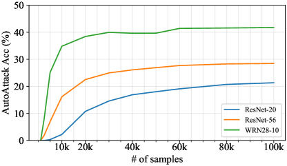
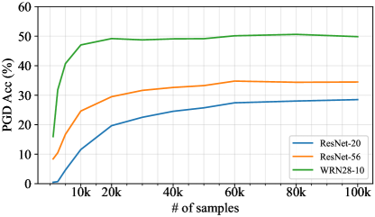
Appendix C Number of Synthetic Samples
In this section, we show the performance gain from simply incrementing the number of synthetic samples. Figure 5 plots the AutoAttack accuracy when trained using differing number of samples. For all models, the trend is similar in that the performance increases linearly, and converge at some point around 50000-60000. Although there exists marginal gain with further supplement of data, we settle for 60000 samples for the training efficiency. One observation is that for smaller model (ResNet-20), it is much harder to obtain meaningful robustness for any set under 20000. We posit this is due to the characteristic of data-free synthesis, where the only guidance is from a pretrained model and the quality of the data is bounded by the performance of the pretrained model. Since larger models tend to learn better representation, it can be reasoned that the smaller models are less capable of synthesizing good quality data, along with the reason that smaller models are generally harder to train for adversarial robustness.
Appendix D Extended Set of Experiments on Medical Datasets
In this section we report an extended version of our experiment on medical datasets, which includes Derma, OCT, OrganA, and OrganS datasets. Table 12 compares DataFreeShield against data-free baseline methods, and Table 13 shows results on test-time defense techniques. Aligned with the observation from Table 3, DataFreeShield is the only method that provides consistently high robustness.
| Model | Method | Derma | OCT | OrganA | OrganS | ||||||||
| RN-18 | Public | 67.48 | 50.47 | 42.39 | 25.60 | 22.00 | 20.90 | 86.79 | 33.82 | 30.28 | 68.82 | 18.25 | 15.41 |
| DaST | 66.93 | 38.35 | 32.72 | 27.00 | 20.70 | 20.50 | 84.42 | 26.07 | 22.70 | 28.55 | 09.40 | 08.82 | |
| DFME | 69.63 | 24.29 | 21.70 | 25.00 | 19.10 | 14.00 | 92.20 | 24.31 | 20.27 | 72.11 | 09.49 | 07.29 | |
| AIT | 66.03 | 35.71 | 33.97 | 21.50 | 11.60 | 09.50 | 70.50 | 11.31 | 08.74 | 50.71 | 13.13 | 08.29 | |
| DFARD | 74.91 | 05.04 | 03.89 | 69.10 | 00.00 | 00.00 | 90.81 | 31.71 | 28.83 | 63.46 | 10.86 | 08.88 | |
| Ours | 66.98 | 63.09 | 61.85 | 31.90 | 23.80 | 18.50 | 86.44 | 49.06 | 44.90 | 64.43 | 29.68 | 24.31 | |
| RN-50 | Public | 67.08 | 44.59 | 34.11 | 25.30 | 22.60 | 19.40 | 78.77 | 33.56 | 28.78 | 47.70 | 12.68 | 04.28 |
| DaST | 72.47 | 08.08 | 04.99 | 25.00 | 05.60 | 00.00 | 64.05 | 17.45 | 15.61 | 53.49 | 08.93 | 05.29 | |
| DFME | 67.08 | 03.19 | 01.10 | 25.00 | 08.40 | 00.00 | 22.42 | 02.58 | 01.82 | 74.50 | 06.93 | 04.21 | |
| AIT | 23.59 | 03.29 | 01.75 | 24.50 | 01.60 | 00.70 | 46.77 | 09.21 | 07.08 | 27.48 | 07.02 | 06.13 | |
| DFARD | 54.02 | 10.97 | 09.23 | 25.50 | 18.50 | 01.30 | 31.37 | 22.60 | 19.82 | 76.09 | 06.33 | 04.07 | |
| Ours | 67.78 | 64.34 | 58.05 | 28.90 | 19.30 | 17.59 | 90.80 | 42.58 | 37.42 | 66.61 | 37.84 | 33.63 | |
| ResNet-18 | ResNet-50 | ||||||
| Dataset | Method | ||||||
| Derma | DAD | 74.51 | 13.47 | 04.24 | 72.02 | 23.79 | 03.39 |
| DiffPure | 65.04 | 55.66 | 28.72 | 68.36 | 59.38 | 45.18 | |
| TTE | 70.47 | 15.81 | 11.62 | 53.57 | 02.29 | 01.10 | |
| Ours | 66.98 | 63.09 | 61.85 | 67.78 | 64.34 | 58.05 | |
| OCT | DAD | 80.20 | 22.90 | 00.20 | 84.50 | 21.70 | 00.00 |
| DiffPure | 30.66 | 26.76 | 09.10 | 28.91 | 29.10 | 16.60 | |
| TTE | 67.10 | 00.00 | 00.00 | 83.30 | 00.00 | 00.00 | |
| Ours | 31.90 | 23.80 | 18.50 | 28.90 | 19.30 | 17.59 | |
| OrganA | DAD | 85.07 | 37.78 | 19.46 | 81.48 | 34.14 | 13.83 |
| DiffPure | 70.12 | 63.48 | 35.94 | 69.34 | 59.96 | 42.79 | |
| TTE | 72.38 | 31.88 | 25.78 | 68.38 | 24.77 | 17.06 | |
| Ours | 86.44 | 49.06 | 44.90 | 90.80 | 42.58 | 37.42 | |
| OrganS | DAD | 47.86 | 29.45 | 05.54 | 57.61 | 30.58 | 05.84 |
| DiffPure | 55.27 | 45.70 | 24.53 | 52.34 | 46.88 | 24.92 | |
| TTE | 61.16 | 05.35 | 02.07 | 53.49 | 09.72 | 03.79 | |
| Ours | 64.43 | 29.68 | 24.31 | 66.61 | 37.84 | 33.63 | |
Appendix E Extended Set of Experiments on -bounds
| ResNet-20 | ResNet-56 | WRN-28-10 | ||||||||
| Method | ||||||||||
| Original | 95.42 | 88.04 | 86.72 | 96.00 | 88.86 | 87.85 | 96.06 | 89.23 | 88.16 | |
| DaST | 93.80 | 34.30 | 12.33 | 91.00 | 46.29 | 31.77 | 96.45 | 35.21 | 09.49 | |
| DFME | 96.05 | 35.24 | 08.39 | 97.30 | 38.79 | 10.98 | 97.21 | 24.67 | 00.54 | |
| AIT | 94.67 | 65.74 | 60.74 | 95.63 | 70.42 | 66.23 | 85.82 | 44.33 | 36.37 | |
| DFARD | 96.58 | 32.64 | 06.89 | 97.29 | 39.21 | 08.94 | 97.11 | 26.38 | 00.29 | |
| DataFreeShield | 94.22 | 75.56 | 72.17 | 94.16 | 80.32 | 78.47 | 95.94 | 84.63 | 82.93 | |
| Original | 93.19 | 78.01 | 74.59 | 94.67 | 79.53 | 79.67 | 94.48 | 79.53 | 76.72 | |
| DaST | 20.66 | 13.90 | 07.06 | 20.20† | 19.59 | 19.65 | 20.15 | 19.17 | 14.57 | |
| DFME | 11.32† | 02.59 | 00.84 | 20.20† | 19.22 | 04.27 | 06.94† | 05.31 | 00.28 | |
| AIT | 91.45 | 37.87 | 24.74 | 86.65 | 45.45 | 38.96 | 83.89 | 40.45 | 33.06 | |
| DFARD | 20.11 | 15.94 | 19.68 | 19.58 | 15.43 | 00.00 | 92.32 | 13.08 | 00.01 | |
| DataFreeShield | 91.83 | 54.82 | 47.55 | 88.66 | 62.05 | 57.54 | 94.14 | 69.60 | 62.66 | |
| Original | 91.47 | 67.39 | 60.56 | 91.59 | 71.10 | 57.95 | 93.62 | 75.03 | 57.36 | |
| DaST | 07.84 | 01.64 | 00.00 | 19.68 | 19.57 | 12.79 | 61.72 | 08.82 | 00.00 | |
| DFME | 15.90† | 15.94 | 14.81 | 97.34 | 05.21 | 00.00 | 97.11 | 01.39 | 00.00 | |
| AIT | 83.70 | 23.20 | 06.03 | 87.23 | 30.06 | 17.37 | 77.05 | 12.45 | 03.61 | |
| DFARD | 24.27 | 19.48 | 00.44 | 97.17 | 05.87 | 00.00 | 54.24 | 19.58 | 00.00 | |
| DataFreeShield | 89.00 | 39.63 | 31.15 | 81.90 | 47.36 | 40.88 | 92.18 | 55.39 | 45.57 | |
| Original | 86.50 | 55.68 | 40.31 | 89.29 | 59.39 | 51.21 | 92.03 | 68.35 | 32.94 | |
| DaST | 10.29 | 03.94 | 02.07 | 19.68† | 19.59 | 19.68 | 20.39 | 16.69 | 01.35 | |
| DFME | 20.15 | 00.30 | 00.00 | 21.55 | 16.60 | 00.22 | 06.84† | 06.70 | 02.29 | |
| AIT | 47.47 | 15.21 | 07.70 | 73.33 | 22.42 | 10.92 | 47.96 | 14.85 | 07.24 | |
| DFARD | 20.03 | 13.46 | 00.00 | 25.18 | 05.46 | 00.00 | 93.07 | 18.23 | 00.02 | |
| DataFreeShield | 85.32 | 29.96 | 20.84 | 75.70 | 37.32 | 29.04 | 90.57 | 43.80 | 31.77 | |
| †Did not converge | ||||||||||
| ResNet-20 | ResNet-56 | WRN-28-10 | ||||||||
| Method | ||||||||||
| Original | 78.82 | 66.59 | 65.53 | 81.01 | 68.34 | 67.42 | 86.34 | 75.39 | 74.81 | |
| DaST | 10.02† | 09.91 | 09.77 | 17.46 | 03.25 | 00.50 | 12.72 | 06.46 | 02.37 | |
| DFME | 32.05 | 09.60 | 04.19 | 91.29 | 16.28 | 00.13 | 97.32 | 18.31 | 00.00 | |
| AIT | 81.25 | 28.90 | 24.72 | 78.51 | 33.66 | 30.25 | 74.05 | 06.66 | 01.27 | |
| DFARD | 91.89 | 07.63 | 00.08 | 95.34 | 16.97 | 00.06 | 97.32 | 10.71 | 00.00 | |
| DataFreeShield | 80.66 | 50.09 | 46.73 | 87.06 | 57.99 | 55.44 | 91.56 | 70.48 | 68.12 | |
| Original | 75.60 | 56.79 | 54.37 | 76.76 | 58.50 | 56.54 | 82.89 | 64.64 | 62.84 | |
| DaST | 10.00† | 09.89 | 08.62 | 12.06 | 07.68 | 05.32 | 10.00† | 09.65 | 02.85 | |
| DFME | 14.36 | 05.23 | 00.08 | 13.81 | 03.92 | 00.03 | 10.00† | 09.98 | 00.05 | |
| AIT | 32.89 | 11.93 | 10.67 | 38.47 | 12.29 | 11.36 | 34.92 | 10.90 | 09.47 | |
| DFARD | 12.28 | 05.33 | 00.00 | 10.84 | 08.93 | 00.00 | 09.82 | 12.01 | 00.02 | |
| DataFreeShield | 74.79 | 29.29 | 22.65 | 81.30 | 35.55 | 30.51 | 86.74 | 51.13 | 43.73 | |
| Original | 70.88 | 48.23 | 45.88 | 73.55 | 50.47 | 47.50 | 77.89 | 54.56 | 52.23 | |
| DaST | 10.00† | 09.86 | 08.02 | 10.00† | 09.00 | 02.21 | 10.17 | 04.97 | 00.07 | |
| DFME | 10.00† | 00.82 | 00.01 | 78.82 | 03.35 | 00.00 | 10.86 | 09.26 | 01.58 | |
| AIT | 24.20 | 07.71 | 03.05 | 22.35 | 09.46 | 07.46 | 63.61 | 03.87 | 00.51 | |
| DFARD | 11.23 | 04.91 | 00.00 | 95.27 | 01.10 | 00.00 | 92.46 | 00.34 | 00.00 | |
| DataFreeShield | 69.11 | 17.94 | 11.03 | 76.55 | 21.55 | 16.11 | 81.26 | 37.26 | 26.07 | |
| Original | 69.19 | 41.69 | 37.30 | 70.79 | 43.89 | 39.97 | 76.76 | 47.88 | 44.04 | |
| DaST | 010.00† | 09.99 | 06.81 | 10.60† | 09.18 | 01.62 | 10.00† | 09.88 | 00.56 | |
| DFME | 13.17 | 01.67 | 00.00 | 10.01† | 02.10 | 00.00 | 10.02† | 04.44 | 00.00 | |
| AIT | 14.02 | 03.49 | 00.28 | 10.06† | 09.97 | 09.96 | 10.12† | 09.66 | 08.16 | |
| DFARD | 11.23 | 01.41 | 00.00 | 13.04 | 03.41 | 00.00 | 10.11 | 09.98 | 00.00 | |
| DataFreeShield | 63.69 | 10.53 | 04.71 | 73.05 | 13.27 | 07.80 | 76.63 | 27.61 | 14.79 | |
| †Did not converge | ||||||||||
In the field of empirical adversarial robustness (Rebuffi et al., 2021; Schmidt et al., 2018; Wang et al., 2019; Wu et al., 2020), thorough evaluation under attacks of varying difficulties (number of iterations, size of , etc) is needed to guarantee the model’s robustness. This is because a consistent trend across different attacks and resistance against strong attacks (AutoAttack) ensures the robustness is not from obfuscated gradients (Athalye et al., 2018). In this regard, we provide further experiment results using diverse set of -bounds using SVHN and CIFAR-10 in Table 14 and Table 15. For each setting, we highlight the best results under .
In both datasets, baseline methods show poor performance regardless of the difficulty of the attack. For example, in CIFAR-10, even at a relatively weaker attack of , DaST, DFME, and DFARD do not exceed 10% under AutoAttack evaluation, which is no better than random guessing. Although AIT performs generally better than the other baselines, it suffers when training a larger model (WRN-28-10). The overall trend of the baselines implies that these methods are unable to learn meaningful robustness, regardless of the size of the distortion. On the other hand, DataFreeShield shows consistent trend across all attacks. While exceeding the baseline methods by a huge margin, the results are stable under both PGD and AutoAttack in all ’s. This shows that DataFreeShield is able to learn meaningful robustness from adversarial training of all presented distortion sizes.
Appendix F Detailed Study on DataFreeShield
We present extended version of detailed study presented in the main paper. Table 16 and Table 17 compare state-of-the-art AT loss functions against our proposed . The results are consistent with what we have displayed in the main paper, where performs the best in almost all settings. Although the other loss functions perform generally well in WRN-28-10, they tend to fall into false sense of security with ResNet-20 and ResNet-56, where the seemingly robust models under weak attacks (PGD) easily break under stronger attacks (AutoAttack). For example, in ResNet-56 of Table 17, STD (Madry et al., 2018) achieves 46.38% under PGD, but is easily circumvented by AutoAttack, which gives 0.12%. Similar phenomenon is observed across other loss functions. However, is consistent under both PGD and AutoAttack, and shows no sign of obfuscated gradients.
| ResNet-20 | ResNet-56 | WRN-28-10 | |||||||
| Method | |||||||||
| STD | 23.34 | 16.73 | 13.83 | 95.12 | 42.66 | 08.73 | 93.71 | 69.32 | 62.58 |
| TRADES | 92.99 | 51.13 | 36.71 | 95.73 | 67.00 | 20.87 | 94.12 | 69.10 | 61.75 |
| MART | 63.36 | 06.48 | 01.98 | 91.65 | 26.09 | 04.74 | 35.94 | 02.55 | 01.09 |
| ARD | 94.78 | 43.10 | 30.38 | 96.02 | 47.37 | 37.16 | 96.29 | 61.11 | 52.56 |
| RSLAD | 93.75 | 44.06 | 29.81 | 94.25 | 56.60 | 48.40 | 96.03 | 64.59 | 57.04 |
| (Proposed) | 91.78 | 54.53 | 45.50 (+8.79) | 91.06 | 63.12 | 56.54 (+8.14) | 94.87 | 69.67 | 65.66 (+3.08) |
| ResNet-20 | ResNet-56 | WRN-28-10 | |||||||
| Method | |||||||||
| STD | 23.51 | 06.09 | 01.66 | 92.49 | 46.38 | 00.12 | 81.63 | 48.03 | 38.94 |
| TRADES | 86.34 | 26.81 | 01.75 | 81.71 | 29.49 | 09.36 | 79.61 | 45.86 | 37.08 |
| MART | 14.91 | 02.67 | 00.22 | 91.65 | 16.23 | 00.00 | 13.69 | 06.74 | 00.09 |
| ARD | 90.13 | 09.83 | 00.17 | 92.21 | 09.31 | 02.51 | 90.95 | 36.61 | 31.16 |
| RSLAD | 77.85 | 11.66 | 00.69 | 88.98 | 19.59 | 12.27 | 90.25 | 39.30 | 31.16 |
| (Proposed) | 77.83 | 27.42 | 19.09 (+17.34) | 83.67 | 34.78 | 27.69 (+15.42) | 88.16 | 50.13 | 41.40 (+2.46) |
For comparison, we present real-data training performance on the medical datasets dataset in Table 18. The ‘original’ data training uses the exact same domain for adversarial training, so that can be regarded as the upper bound of the data-free adversarial robustness. The experimental results show that even real data from another domain (CIFAR-10) significantly underperform compared to the original dataset. On the other hand, DataFreeShield shows superior performance than the other-domain public dataset. Remarkably, DataFreeShield almost reached similar performance levels with the original dataset training in the Derma dataset. The experimental results show the advantages of DataFreeShield, by reducing the gap towards real-data training.
| Dataset | Data-free | Method | ResNet-18 | ResNet-50 | ||||
| Tissue | ✗ | Original | 50.33 | 37.53 | 34.25 | 48.94 | 37.34 | 35.06 |
| Public (CIFAR-10) | 22.04 | 00.02 | 00.00 | 27.84 | 10.11 | 08.64 | ||
| ✓ | DataFreeShield | 32.07 | 31.63 | 31.57 | 31.91 | 27.15 | 26.68 | |
| Blood | ✗ | Original | 86.73 | 71.94 | 70.36 | 85.41 | 71.79 | 70.51 |
| Public (CIFAR-10) | 09.09 | 09.09 | 00.00 | 09.09 | 09.09 | 00.00 | ||
| ✓ | DataFreeShield | 59.89 | 21.72 | 19.29 | 74.63 | 36.07 | 30.17 | |
| Path | ✗ | Original | 74.37 | 52.53 | 49.35 | 72.62 | 51.73 | 48.68 |
| Public (CIFAR-10) | 13.30 | 00.00 | 00.00 | 07.54 | 01.21 | 00.37 | ||
| ✓ | DataFreeShield | 33.06 | 29.78 | 25.38 | 41.63 | 15.35 | 12.28 | |
| Derma | ✗ | Original | 66.90 | 63.90 | 63.01 | 67.58 | 61.99 | 60.14 |
| Public (CIFAR-10) | 67.48 | 50.47 | 42.39 | 67.08 | 44.59 | 34.11 | ||
| ✓ | DataFreeShield | 66.98 | 63.09 | 61.85 | 67.78 | 64.34 | 58.05 | |
| OrganA | ✗ | Original | 92.79 | 81.20 | 80.75 | 92.67 | 82.73 | 82.25 |
| Public (CIFAR-10) | 86.79 | 33.82 | 30.28 | 78.77 | 33.56 | 28.78 | ||
| ✓ | DataFreeShield | 86.44 | 49.06 | 44.90 | 90.80 | 42.58 | 37.42 | |
| OrganC | ✗ | Original | 91.13 | 81.06 | 80.55 | 90.52 | 81.47 | 80.94 |
| Public (CIFAR-10) | 79.41 | 40.10 | 36.53 | 84.41 | 46.12 | 43.44 | ||
| ✓ | DataFreeShield | 83.35 | 47.01 | 42.56 | 86.56 | 62.60 | 59.86 | |
| OrganS | ✗ | Original | 79.01 | 62.62 | 61.95 | 79.08 | 65.16 | 64.57 |
| Public (CIFAR-10) | 68.82 | 18.25 | 15.41 | 47.70 | 12.68 | 04.28 | ||
| ✓ | DataFreeShield | 64.43 | 29.68 | 24.31 | 66.61 | 37.84 | 33.63 | |
Similarly, for dataset diversification, we show an extended version in Table 19 and Table 20. In all settings, diversified sample synthesis shows the best quantitative measure under Coverage and JSD. Coverage is known to be a more accurate measure of diversity than Recall in the sense that it is more robust against outliers (Naeem et al., 2020). Also, JSD measures distributional distance, which is frequently used in evaluating GANs. Thus, they show quantitative evidence to diversity gain of diversified sample synthesis. This aligns with the robust training results, where diversified sample synthesis outperforms other diversifying methods in most settings.
| Accuracy | Diversity Metric | |||||||
| Model | Method | Recall | Coverage | NDB | JSD | |||
| ResNet-20 | 93.31 | 54.11 | 41.03 | 0.801 | 0.230 | 95 | 0.353 | |
| + Mixup | 92.13 | 57.71 | 48.17 (+7.14) | 0.882 | 0.241 | 88 | 0.368 | |
| + Cutout | 91.34 | 56.01 | 48.29 (+7.26) | 0.900 | 0.198 | 90 | 0.396 | |
| + CutMix | 92.06 | 56.79 | 48.14 (+7.11) | 0.887 | 0.225 | 91 | 0.387 | |
| + DSS | 91.78 | 54.53 | 45.50 (+4.47) | 0.905 | 0.429 | 90 | 0.237 | |
| ResNet-56 | 93.17 | 61.40 | 54.38 | 0.821 | 0.218 | 93 | 0.342 | |
| + Mixup | 92.23 | 62.26 | 55.11 (+0.73) | 0.848 | 0.226 | 93 | 0.345 | |
| + Cutout | 93.92 | 60.54 | 53.80 (-0.58) | 0.842 | 0.164 | 95 | 0.391 | |
| + CutMix | 91.20 | 61.46 | 55.38 (-1.00) | 0.871 | 0.189 | 95 | 0.369 | |
| + DSS | 91.06 | 63.12 | 56.54 (+2.16) | 0.872 | 0.521 | 93 | 0.154 | |
| WRN-28-10 | 94.26 | 64.94 | 59.99 | 0.246 | 0.147 | 91 | 0.254 | |
| + Mixup | 94.50 | 67.51 | 54.70 (-5.29) | 0.252 | 0.120 | 94 | 0.277 | |
| + Cutout | 95.51 | 66.77 | 61.96 (+1.97) | 0.305 | 0.060 | 91 | 0.332 | |
| + CutMix | 95.67 | 66.71 | 61.16 (+1.17) | 0.321 | 0.100 | 92 | 0.348 | |
| + DSS | 94.87 | 69.67 | 65.66 (+5.67) | 0.548 | 0.232 | 88 | 0.190 | |
| Accuracy | Diversity Metric | |||||||
| Model | Method | Recall | Coverage | NDB | JSD | |||
| ResNet-20 | 82.58 | 23.93 | 14.61 | 0.400 | 0.107 | 88 | 0.355 | |
| + Mixup | 84.26 | 16.91 | 05.95 (-8.66) | 0.692 | 0.128 | 87 | 0.372 | |
| + Cutout | 82.65 | 26.33 | 17.32 (+2.71) | 0.747 | 0.137 | 95 | 0.369 | |
| + CutMix | 83.38 | 28.66 | 18.30 (+3.69) | 0.825 | 0.175 | 89 | 0.347 | |
| + DSS | 77.83 | 27.42 | 19.09 (+4.48) | 0.724 | 0.320 | 90 | 0.248 | |
| ResNet-56 | 83.72 | 30.91 | 27.42 | 0.658 | 0.136 | 93 | 0.310 | |
| + Mixup | 83.55 | 32.87 | 27.87 (+0.45) | 0.761 | 0.135 | 93 | 0.394 | |
| + Cutout | 82.96 | 31.39 | 26.83 (-0.59) | 0.853 | 0.113 | 94 | 0.343 | |
| + CutMix | 82.60 | 33.78 | 27.86 (+0.44) | 0.892 | 0.150 | 93 | 0.364 | |
| + DSS | 83.67 | 34.78 | 27.69 (+0.27) | 0.678 | 0.550 | 84 | 0.126 | |
| WRN-28-10 | 91.46 | 43.66 | 36.34 | 0.535 | 0.101 | 91 | 0.253 | |
| + Mixup | 90.61 | 48.16 | 36.43 (+0.09) | 0.641 | 0.084 | 94 | 0.322 | |
| + Cutout | 92.59 | 39.84 | 34.39 (-1.95) | 0.535 | 0.034 | 95 | 0.443 | |
| + CutMix | 91.90 | 42.79 | 34.79 (-1.55) | 0.845 | 0.084 | 93 | 0.328 | |
| + DSS | 88.16 | 50.13 | 41.40 (+5.06) | 0.830 | 0.163 | 88 | 0.211 | |
Appendix G Evaluation under Modified Attacks
| Dataset | Model | Modified Attack | ||||||
| SVHN | ResNet-20 | 91.83 | 54.82 | 47.55 | 74.38 | 71.95 | 55.84 | 55.24 |
| ResNet-56 | 88.66 | 62.05 | 57.54 | 77.99 | 77.04 | 62.95 | 62.58 | |
| WRN-28-10 | 94.14 | 69.60 | 62.66 | 87.68 | 81.39 | 70.64 | 70.08 | |
| CIFAR-10 | ResNet-20 | 74.79 | 29.29 | 22.65 | 65.63 | 54.64 | 31.05 | 30.46 |
| ResNet-56 | 81.30 | 35.55 | 30.51 | 67.73 | 60.61 | 36.94 | 36.43 | |
| WRN-28-10 | 86.74 | 51.13 | 43.73 | 79.38 | 70.40 | 51.82 | 51.21 | |
| Dataset | Model | Modified Attack | ||||||
| Tissue | ResNet-18 | 32.07 | 31.93 | 31.83 | 32.07 | 31.98 | 31.95 | 31.95 |
| Blood | 49.34 | 19.24 | 18.77 | 20.32 | 29.87 | 24.70 | 24.12 | |
| Path | 33.06 | 29.78 | 25.38 | 29.81 | 32.10 | 30.04 | 29.99 | |
| OrganC | 76.89 | 46.92 | 45.18 | 76.60 | 65.47 | 48.40 | 48.10 | |
Evaluating robust accuracy using PGD (Madry et al., 2018) and AutoAttack (Croce & Hein, 2020) are considered de facto standard to demonstrate the method’s robustness. However, we extend our experiments and provide further evaluation under latent attack (Sabour et al., 2016) and using different combinations of our training loss as the inner maximization of PGD. We term these attacks modified attacks because they are modified according to the training objective or takes advantage of model architecture to generate adversarial samples, similar to adaptive attacks (Liu et al., 2022; Yao et al., 2021). For modified versions of PGD, each replaces the coventionally used cross entropy loss with: (a) , (b) , (c) . For latent attack (Sabour et al., 2016), we followed the original implementation and used output from the penultimate layer (before flattening), L-BFGS for attack optimization with =10/255 for perturbation bound. The results are shown in Table 21 and Table 22, where our method DataFreeShield is effective against modified attacks as well. In all datasets and models, none of the modified attack methods were stronger than cross entropy based PGD and AutoAttack.
Appendix H Further Visualization of Loss Surface
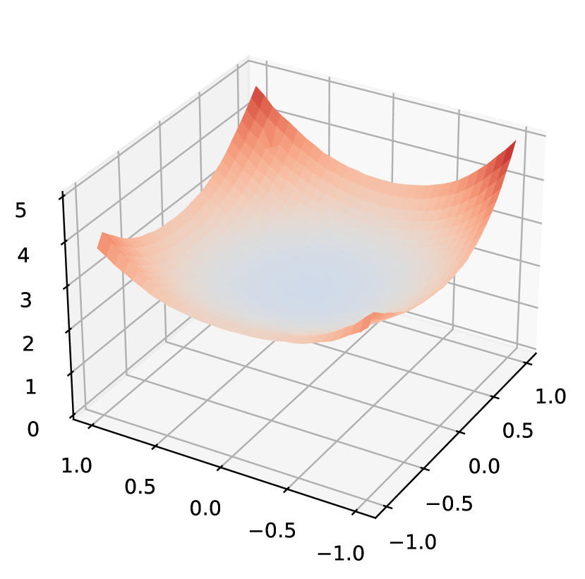
w/o GradRefine
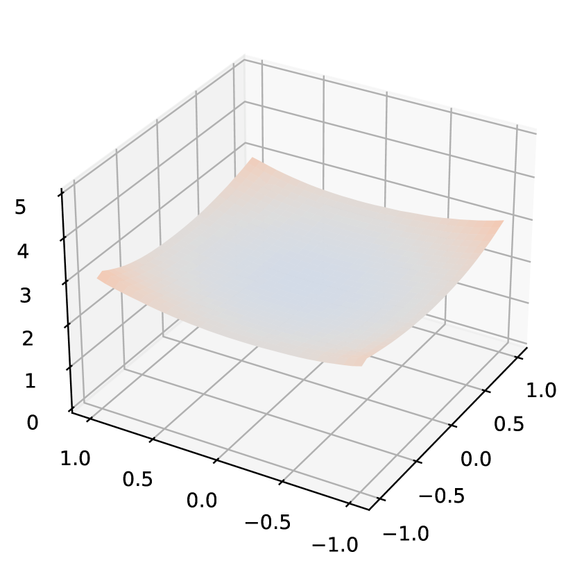
w/ GradRefine
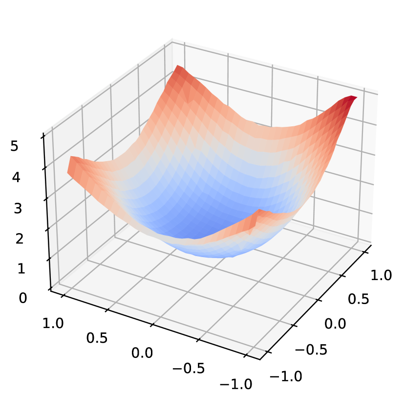
w/o GradRefine
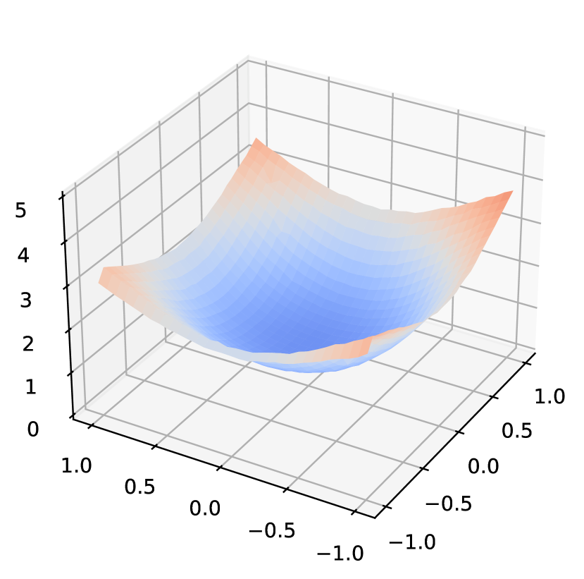
w/ GradRefine
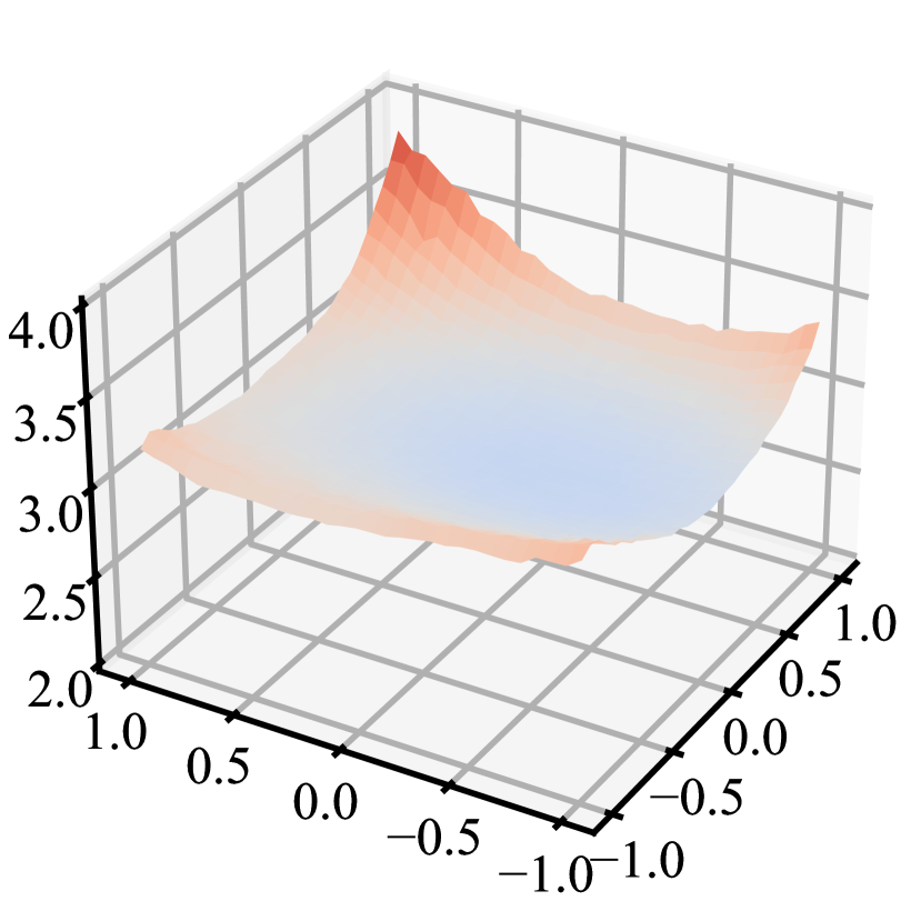
w/o GradRefine
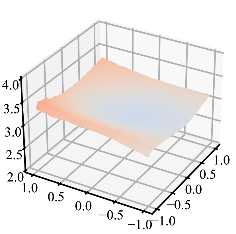
w/ GradRefine
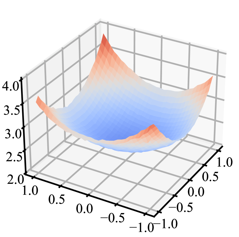
w/o GradRefine
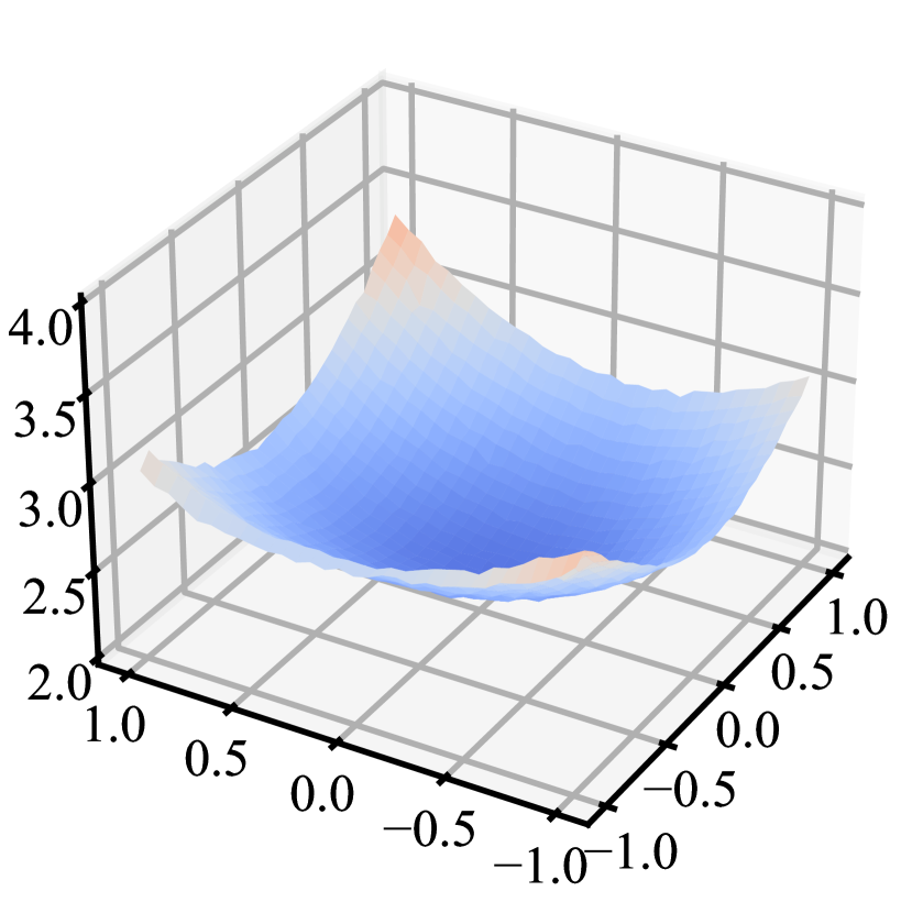
w/ GradRefine
We extend Figure 4 to different models, ResNet-56 and WRN-28-10. The visualization results are shown in Figures 6 and 7. In all visualization settings, applying GradRefine to data-free adversarial training achieves a flatter loss surface. This analysis further supports the experimental results that GradRefine contributes to better performance.
Appendix I Sensitivity Study on the Number of Aggregated Batches
| ResNet-20 | WRN-28-10 | |||||
| 1 | 77.83 | 27.42 | 19.09 | 88.16 | 50.13 | 41.40 |
| 2 | 75.77 | 29.16 | 22.44 | 88.07 | 50.50 | 41.96 |
| 4 | 74.74 | 29.19 | 22.94 | 87.85 | 50.36 | 42.10 |
| 8 | 75.01 | 29.47 | 23.09 | 87.67 | 50.53 | 41.80 |
| 10 | 75.53 | 29.69 | 22.95 | 87.65 | 50.75 | 42.35 |
| 20 | 74.63 | 29.28 | 22.63 | 86.74 | 51.13 | 43.73 |
| 40 | 28.87 | 13.72 | 10.35 | 85.48 | 50.39 | 44.43 |
In this section, we show a sensitivity study on the number of aggregated batches when applying GradRefine. Table 23 shows the performance under varying number of aggregated batches () during training. Aggregated batch being 1 means GradRefine was not applied. For both models, we can observe that the performance is relatively stable for a wide range of . Also, a smaller model displays slightly higher sensitivity towards , while a larger model is less affected by it. We found to work generally well across different datasets and models.
Appendix J Sensitivity Study on
| SVHN | CIFAR-10 | |||||
| 0.0 | 93.69 | 69.05 | 61.99 | 88.16 | 50.13 | 41.40 |
| 0.1 | 93.65 | 68.78 | 61.98 | 86.94 | 50.29 | 42.17 |
| 0.2 | 93.66 | 68.83 | 62.96 | 86.95 | 50.12 | 42.06 |
| 0.3 | 93.86 | 69.13 | 63.13 | 87.53 | 50.63 | 42.93 |
| 0.4 | 94.05 | 69.12 | 63.17 | 87.13 | 50.99 | 43.34 |
| 0.5 | 94.14 | 69.60 | 62.66 | 86.74 | 51.13 | 43.73 |
| 0.6 | 94.38 | 70.09 | 63.52 | 87.17 | 51.58 | 43.62 |
| 0.7 | 94.69 | 70.13 | 62.77 | 87.10 | 51.96 | 43.84 |
| 0.8 | 95.00 | 69.90 | 61.85 | 86.83 | 51.87 | 43.10 |
| 0.9 | 95.01 | 69.72 | 61.37 | 86.82 | 50.67 | 41.38 |
| 1.0 | 95.42 | 69.10 | 59.45 | 88.10 | 49.11 | 39.12 |
In this section, we provide sensitivity study results on the threshold value used in GradRefine, which is displayed in Table 24. In general, the best range for lies in , with more degradation when being close to 0.0 and 1.0. In all settings, we simply use for the difference within the best range is insignificant. Note that in our method, means no masking is used (allow conflicting gradients), and means all gradients are masked unless they all have the same sign direction. Intuitively, values close to 0.0 diminish the effect of masking, and values close to 1.0 set an unrealistic high bar for gradients, where both should have a negative effect on the final performance.
Appendix K Sensitivity Study on and
| 0 | 0.01 | 0.1 | 1 | 10 | 100 | ||
| Model | () | () | () | () | () | () | |
| ResNet-20 | 0 | 0.04 (96.59) | 0.11 (96.55) | 45.16 (93.10) | 44.55 (72.21) | 19.59 (19.59) | 6.70 (6.70) |
| 0.01 | 0.14 (96.64) | 1.23 (96.70) | 44.36 (93.52) | 47.99 (78.43) | 19.59 (19.59) | 6.70 (6.70) | |
| 0.1 | 40.69 (93.12) | 40.58 (93.63) | 43.82 (93.20) | 51.50 (88.24) | 19.59 (19.59) | 6.70 (6.70) | |
| 1 | 42.95 (93.75) | 42.80 (93.69) | 43.25 (93.78) | 47.55 (91.83) | 19.56 (19.62) | 6.70 (6.70) | |
| 10 | 42.63 (87.56) | 42.07 (86.39) | 43.34 (88.56) | 45.74 (86.45) | 38.78 (80.30) | 6.70 (6.70) | |
| 100 | 6.70 (6.70) | 6.70 (6.70) | 6.70 (6.70) | 6.70 (6.70) | 6.70 (6.70) | 6.70 (6.70) | |
| ResNet-56 | 0 | 0.18 (97.22) | 2.31 (97.31) | 48.79 (93.58) | 52.53 (73.34) | 19.59 (19.59) | 6.70 (6.70) |
| 0.01 | 3.36 (97.28) | 11.21 (97.08) | 49.17 (93.71) | 54.71 (76.90) | 19.63 (19.69) | 6.70 (6.70) | |
| 0.1 | 43.14 (95.04) | 45.01 (94.22) | 51.97 (93.72) | 58.01 (84.51) | 22.55 (25.50) | 6.70 (6.70) | |
| 1 | 55.56 (91.94) | 55.59 (91.96) | 56.01 (91.55) | 57.54 (88.66) | 50.97 (76.66) | 6.70 (6.70) | |
| 10 | 53.22 (85.85) | 53.44 (86.15) | 53.57 (85.57) | 53.36 (84.65) | 51.06 (84.01) | 10.86 (14.79) | |
| 100 | 37.96 (72.76) | 33.70 (72.88) | 36.11 (73.93) | 37.28 (75.71) | 38.67 (70.18) | 6.70 (6.70) | |
| WRN-28-10 | 0 | 0.22 (97.39) | 0.61 (97.43) | 60.42 (95.49) | 56.30 (83.42) | 21.51 (25.21) | 19.59 (19.59) |
| 0.01 | 0.69 (97.44) | 1.38 (97.45) | 60.56 (95.53) | 59.14 (86.00) | 22.12 (28.83) | 19.59 (19.59) | |
| 0.1 | 27.62 (96.37) | 41.93 (96.27) | 61.03 (95.59) | 63.53 (91.75) | 40.85 (58.79) | 19.59 (19.59) | |
| 1 | 60.72 (95.41) | 60.74 (95.39) | 61.16 (95.21) | 62.66 (94.14) | 58.56 (86.35) | 19.59 (19.59) | |
| 10 | 60.15 (92.45) | 60.05 (92.52) | 60.13 (92.59) | 60.00 (92.09) | 57.75 (88.38) | 38.88 (67.03) | |
| 100 | 44.95 (81.76) | 46.19 (83.62) | 44.45 (81.28) | 46.14 (82.94) | 45.38 (82.58) | 43.35 (76.67) | |
| 0 | 0.01 | 0.1 | 1 | 10 | 100 | ||
| Model | () | () | () | () | () | () | |
| ResNet-20 | 0 | 0.00 (93.99) | 0.00 (93.79) | 18.06 (82.92) | 20.31 (67.61) | 9.26 (13.16) | 10.00 (10.00) |
| 0.01 | 0.00 (93.62) | 0.00 (93.46) | 18.84 (82.47) | 21.18 (68.99) | 10.43 (13.05) | 10.00 (10.00) | |
| 0.1 | 10.36 (86.44) | 12.32 (85.20) | 20.72 (80.33) | 24.20 (72.44) | 11.45 (14.84) | 10.00 (10.00) | |
| 1 | 20.83 (78.49) | 20.69 (78.59) | 21.27 (78.24) | 22.65 (74.79) | 12.53 (15.75) | 10.00 (10.00) | |
| 10 | 15.74 (63.26) | 15.82 (61.62) | 14.59 (61.58) | 14.20 (53.02) | 12.31 (36.82) | 10.00 (10.00) | |
| 100 | 10.00 (10.00) | 10.00 (10.00) | 10.00 (10.00) | 10.00 (10.00) | 10.00 (10.00) | 10.00 (10.00) | |
| ResNet-56 | 0 | 0.00 (95.44) | 0.00 (94.67) | 24.81 (87.04) | 32.09 (78.33) | 11.44 (16.22) | 10.00 (10.00) |
| 0.01 | 0.00 (94.70) | 0.00 (94.81) | 25.31 (86.78) | 32.62 (78.89) | 11.04 (16.13) | 9.65 (11.35) | |
| 0.1 | 19.83 (88.73) | 21.18 (88.23) | 25.65 (85.71) | 33.08 (79.65) | 9.93 (23.06) | 9.00 (14.57) | |
| 1 | 26.71 (84.31) | 26.96 (84.43) | 27.44 (83.92) | 30.51 (81.30) | 24.07 (58.25) | 15.49 (16.49) | |
| 10 | 26.01 (74.59) | 26.22 (74.67) | 25.50 (74.72) | 25.87 (72.84) | 22.91 (61.85) | 10.00 (10.00) | |
| 100 | 10.00 (10.00) | 10.00 (10.00) | 10.00 (10.00) | 10.00 (10.00) | 10.00 (10.00) | 10.00 (10.00) | |
| WRN-28-10 | 0 | 0.00 (97.48) | 0.00 (97.34) | 33.06 (92.61) | 45.08 (82.11) | 12.99 (16.15) | 7.93 (11.38) |
| 0.01 | 0.00 (97.35) | 0.00 (97.27) | 34.29 (92.13) | 45.16 (82.75) | 13.22 (17.05) | 10.00 (10.00) | |
| 0.1 | 28.13 (92.89) | 30.14 (92.52) | 38.44 (91.27) | 44.70 (84.01) | 29.47 (54.82) | 10.00 (10.00) | |
| 1 | 40.46 (89.47) | 40.43 (89.45) | 41.05 (89.26) | 43.73 (86.74) | 39.47 (71.48) | 14.91 (20.84) | |
| 10 | 41.47 (86.28) | 41.32 (85.52) | 40.73 (85.40) | 41.22 (84.81) | 38.62 (78.42) | 19.19 (42.60) | |
| 100 | 15.75 (50.55) | 16.64 (50.05) | 18.02 (51.54) | 18.29 (51.75) | 18.07 (53.38) | 17.68 (51.48) | |
In this section we show a sensitivity study on hyperparameters of by varying the scale of and from 0 to 100.0. The results for SVHN and CIFAR-10 are shown in Table 25 and Table 26, respectively. In general, setting both and as 1.0 performs well regardless of the model and dataset. Although there exist a few cases where increasing or yields better robust accuracy, they all come at the price of large degradation in clean accuracy. As noted in the main body of the paper, we found setting both values to 1.0 best balances such trade-off, while maintaining high robust accuracy.
Appendix L Visualization of DSS using PCA
In this section we provide feature visualization using PCA on CIFAR-10 dataset to conduct similar visualization as done in Figure 3 but on a high-dimensional image dataset. Using all model architectures, Figure 8(c) demonstrates the efficacy of DSS in increasing dataset diversity. DSS shows larger coverage in terms of diversity than when using fixed coefficients, aligning with previous results on toy example (Figure 3). This shows that DSS can effectively enlarge diversity even in complex, real-world datasets. We also visualize the case of high and low by setting each hyperparameter to 1.0 and 0.0. While high generates samples with more distinct class information, they are highly clustered to the class centers. However, absence of loses class information essential to classification tasks. While fixed coefficients strive to find a good balance between these terms with negligence of diversity, DSS successfully achieves both.
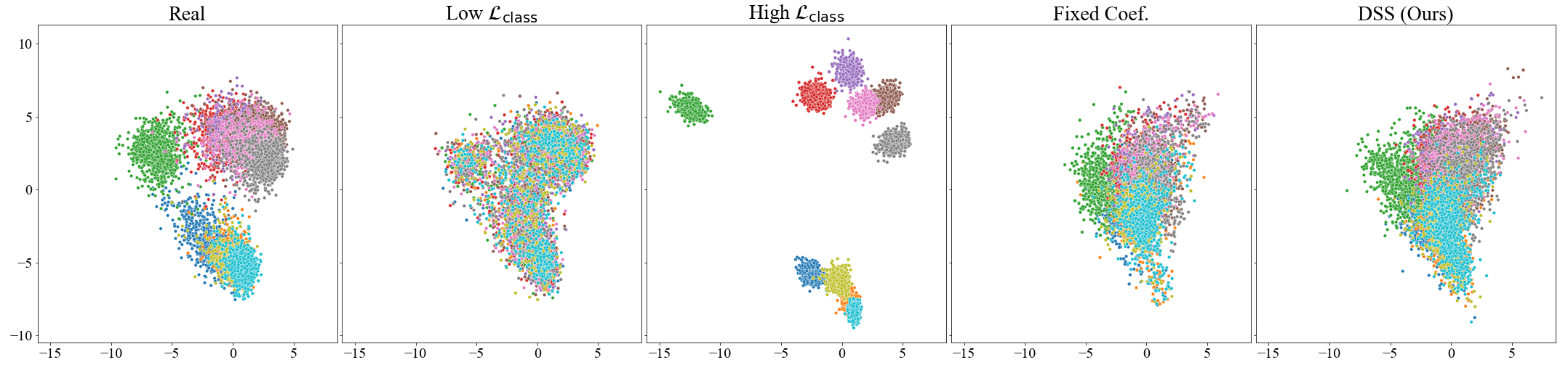
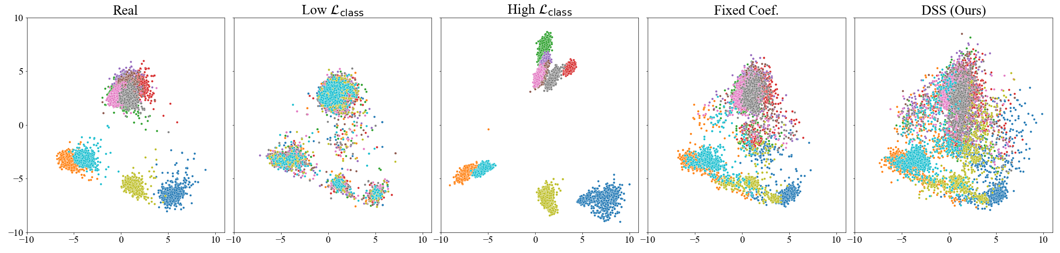

Appendix M Generated Synthetic Samples
In this section, we display generated synthetic samples used in our experiments, including the baseline methods. The resulting images are displayed in Figure 9 to Figure 14. The overall quality of the baseline samples are noticeably poor, with limited diversity and fidelity. While these images are sufficient for specific tasks such as knowledge distillation or model compression, they are unable to give the necessary amount of information needed in robust training. On the other hand, diversified sample synthesis is able to generate diverse samples that are also high in fidelity. For example, in Figure 10 and Figure 11, diversified sample synthesis restores colors and shapes of the original data, while also generating non-overlapping, diversified set of examples. Also, for SVHN, diversified sample synthesis is the only method that is able to generate readable numbers that are recognizable to human eyes. Even in CIFAR-10, a dataset with more complex features, diversified sample synthesis generates samples that faithfully restore the knowledge learned from the original dataset. For larger models with more capacity, the generated samples show recognizable objects such as dogs, airplanes, frogs, etc. The difference in the quality of the generated samples, in addition to the experiment results show that fidelity and diversity of train data play crucial roles in robust training.