Optimization of Trajectories for Machine Learning Training in Robot Accuracy Modeling

I Introduction

Among the exciting applications of Machine Learning (ML) in robot control is the possibility of increasing the accuracy of flexible and friction-prone control of robotic joints in elongated mechanisms. Surgical instruments are an extreme example of robotic end effectors which require a very high length to thickness aspect ratio of the links (especially more distal links). This premium is especially marked for endoscopic surgical instruments as in the daVinci surgical robotic system from Intuitive Surgical Inc.

With long thin mechanisms, in which it is impractical to mount actuators directly on the joints (also a property of robotic surgical instruments), transmission elements undergo large strains and stresses. Elements such as cables, torsion rods, and associated pullies and tiny bearings inevitably introduce properties such as elastic deformation and backlash (position error), and friction. Friction can be though of as velocity dependent force. At the low speeds typical of robotic surgical applications, friction forces are large and highly non-linear.

Machine learning has been recently applied to model these effects. To train such models a robot is moved through various training points, and ground truth position and force data are acquired through high accuracy sensors of the robot’s end-point [1, 2, 3, 4].

It is well known that modern ML methods require large sets of training data and that acquisition of useful training data sets from real physical robots is expensive. A workspace target is defined (seldom as big as the full robot’s work volume) and it can be filled with random points or a regular grid of points. Training data must be collected with the robot posed in each of these points. Since friction varies with velocity, to fully characterize the mechanism we must also select velocities and visit each of the positions at each of the velocities. This can easily grow to a very large number of points, but it takes time and energy for the robot to move between these points and velocities.

Given a set of points in space, and a set of velocities in the same space, we define the phase space as the combined space of positions and velocities.

We can summarize the problem of this paper as: Given a set of points in a phase space, what is the lowest cost trajectory through the phase space which visits each point exactly once? For a trajectory between two points in phase space, we define cost in this paper as either the duration of the trajectory or the energy of the trajectory.

This is of course a variation of the Traveling Salesman Problem.

I-A Goals

Specifically, the goals are

• Study the difficulty of the TSP in this application by applying it to $X,Y,Z$ motion in 3D space ($6D$ phase space).

• Assess the effectiveness of an extremely simple Nearest Neighbor (’NN’) search algorithm compared to random sampling of the search space.

I-B Approach

In this work we will study a practical ‘Nearest Neighbor’[5] heuristic search for this special case of the TSP we will designate as “NN”. For simplicity (and because it seems to obtain good results) we study the simple heuristic algorithm which when building a path from a starting point, chooses a random branch from among a set of branches found to have approximately the lowest cost value (within 2%) among all unvisited nodes. There are many improvements on this heuristic algorithm (reviewed in [5, 6, 7]) and we assume that some of them could further improve our results.

I-C Literature Review

Recent work has applied ML to the problem of increasing the accuracy of controlling manipulators with adverse mechanical properties such as flexibility and friction in transmission components[1, 2, 3, 4]. All of this work relies on training data collected from programmed robot motion - inherently a slow process. Since mechanical properties change with wear and usage, repeated training during the robot’s lifetime is desirable.

Assuming that there is a set of points in space, and discrete velocities, which could sample the robot’s workspace adequately for ML correction, we need to visit those points as fast as possible. The TSP is one approach to optimizing the visiting of training points.

The TSP is a very well studied problem with many applications in, for example, logistics, machine scheduling, PC board drilling, and X-ray crystallography[7]. Notably, [8] applied TSP to motion control of a 3-axis mechanical X-ray source in order to collect the required images as efficiently as possible. However this application requires 0 velocity at each point and is symmetric.

TSP computational approaches have been recently reviewed in [9, 7]. Most often, the TSP is studied in 2D Euclidian space with symmetric costs (such as physical distance) between nodes.

Few papers seem to have studied a TSP in which points share components between position and velocity (phase space). An exception is [10] which derives theoretical lower bounds for a class of TSPs that includes double integrator systems which are somewhat representative of the system used here. Because of the linkage between position and velocity, trajectories in phase space between two points must be asymmetric.

II Methods

We verified that our problem is asymmetric by computing that randomized phase space trajectories differed in cost depending on the direction of travel between two points. [6] reviews the added difficulties imposed by this complexity. Using the energy cost but not the time cost (see below) the problem is non-Euclidean because with the energy cost, we found many point-triplets in phase space for which the triangle inequality did not hold[11].

Trajectories between points were synthesized by fitting a 3rd order polynomial to the starting and ending position and velocity (Section V). The speed of each trajectory was scaled such that the maximum acceleration was $A_{max}=2$.

II-A Spaces

Computational complexity of the TSP grows extremely quickly. We consider grids of $N$ points on each axis normalized to $[-1,-1]$. The simplest case is a 2D space with $N$ positions along a line, and $N$ velocities at each point. A more realistic case is a 6D space consisting of $X,Y,Z$ position axes and $\dot{X},\dot{Y},\dot{Z}$ velocity axes. We will focus our work on these 2D and 6D cases.

We then must visit $N^{m}$ points where $m$ is even (in our case 2 or 6). There are $N^{m}$ possible starting points and then $N^{m}-1$ possibilities for the second point, etc. Thus there are factorial($N^{m}$) possible paths. For 2D, $m=2,N=3$, we have 9 points and 362880 possible paths. This allows for exhaustive search resulting in a global optimum result. For $N=4$ this balloons to 20922789888000 ($2.092\times 10^{13}$). Using the computation time that our generic PC took to search 362880 paths, the predicted time for the 2D, $N=4$ exhaustive search was 220 years(!). For $N=3,m=6$, however the number of paths is $1.4394420\times 10^{1772}$ . So, except for $N=3,m=2$ exhaustive search is not feasible. Although our code was in unoptimized Python 3, allowing for a 100x speedup for C-based code still predicts daunting runtimes.

Initially we studied rectangular grids of points, equally spaced in position and velocity. To determine if there were special features of optimal trajectories on rectangular grids, we did additional computations on random grids. These were generated off line and stored in a file so that comparisons between different search methods could be made on the same random grid.

We will then study 4 spaces, 2D rectangular, 2D random, 6D rectangular, 6D random. In some cases, computations on the random grid were repeated on different random grids to confirm observed effects were not due to a specific random configuration but results were very similar.

II-B Code and computing

Trajectory generation, cost evaluation, nearest-neighbor (NN) heuristic searching, exhaustive searching, and random path sampling were coded in Python3 with (among others) the numpy and itertools libraries. Full source code is available on Github.

Heuristic Search, Starting point dependence

Heuristic NN searches produce a result which can depend on starting point. In our application, a robot must be initialized and then incur a small cost (compared to the overall trajectory cost) to move to the starting point selected for an optimal path. However we will consider all starting points equally.

For the 2D, 4x4 grid there are 16 starting points and for the 6D, 4x4 grid there are $4^{6}=4096$ starting points.

As above, if during the NN search, branch costs were within 2% of the lowest cost branch, they were considered equal and one was chosen randomly each time. The largest tie (set of paths within 2% of optimium time cost) encountered during the 4x4 rectangular NN time-cost search was 56 branches.

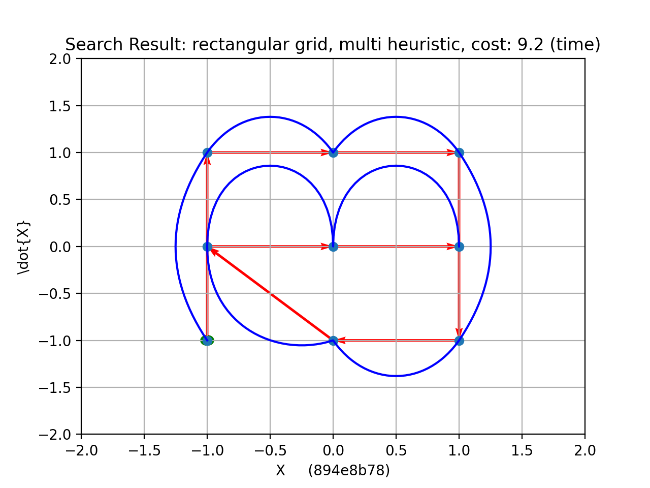
(a) Suboptimal: Time Cost

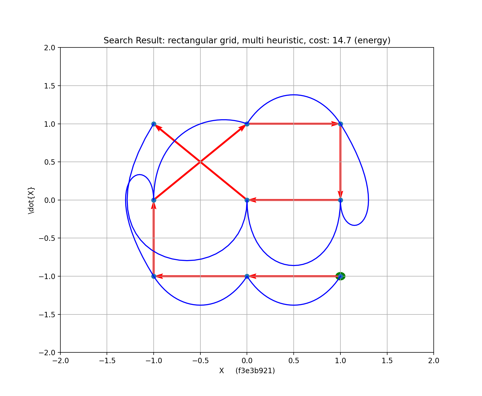
(b) Suboptimal: Energy Cost

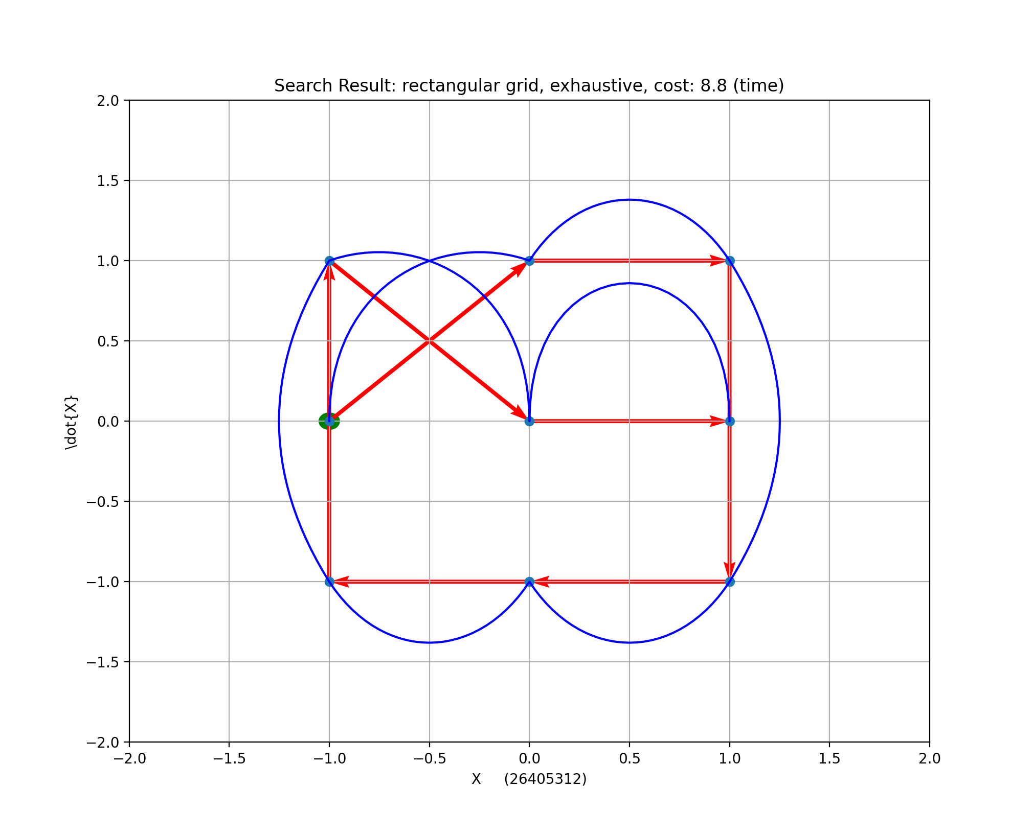
(c) Globally optimal: Time Cost

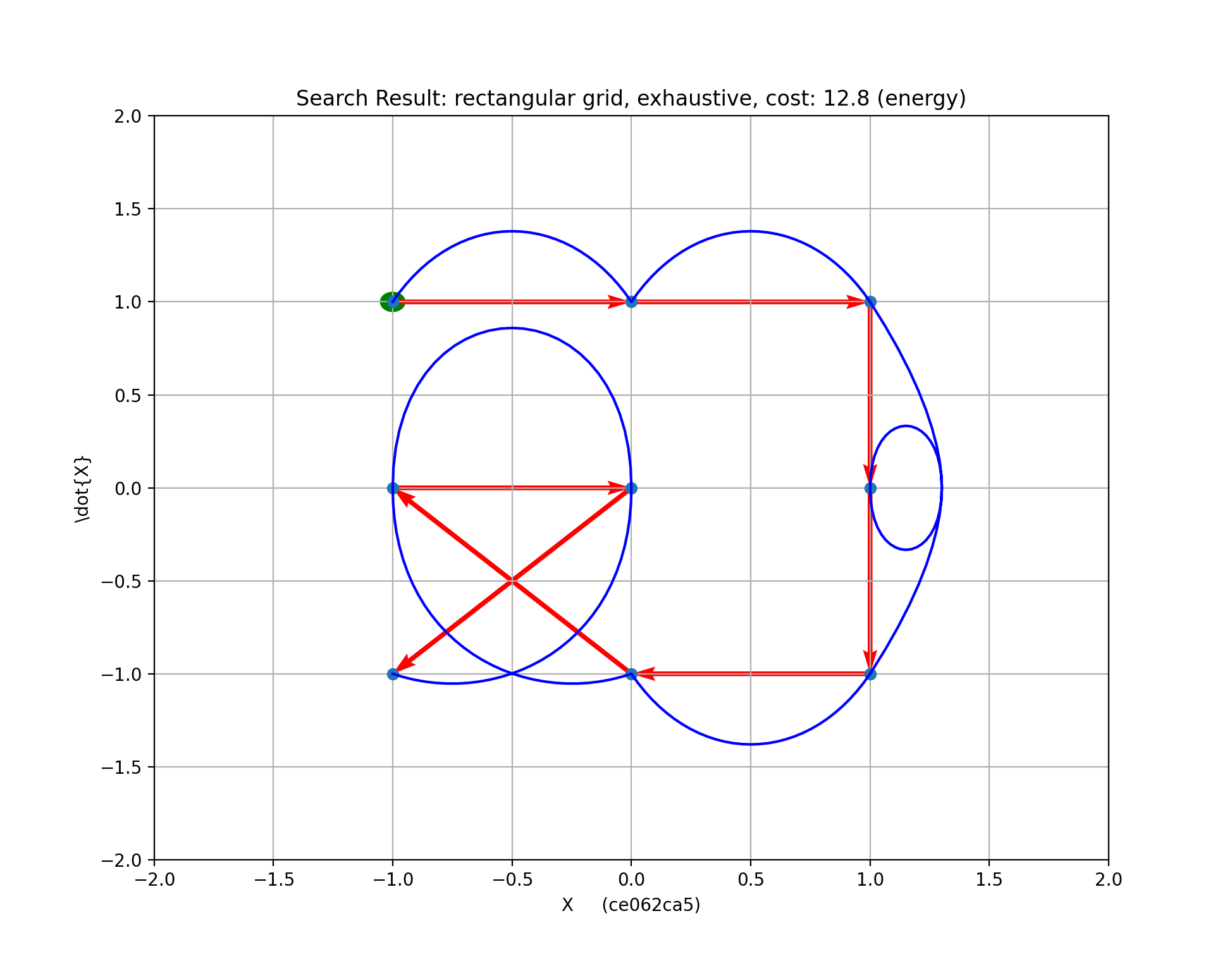
(d) Globally optimal: Energy Cost

Figure 1: 2D, 3x3 searches, rectangular grid. a,b: Suboptimal paths, found by heuristic search (using only 4 starting points). Starting point is enlarged green circle. Red arrows show sequence of points, blue curves are the solved trajectories (Section V-B, Fig. 16). c,d: Globally optimal path on 3x3 grid found by exhaustive searches. Hash codes identify pertinent data files.

III Results

III-A 2D, $N=3$

III-A1 Rectangular Grid

Our first result is a very quick search using only 4 starting points of the 9 possible in the 2D, $N=3$ space and the NN search. This was expected to get suboptimal trajectories (Figure 1 top row). Because of the sign convention in phase space, individual point-to-point trajectories tend to go in clockwise loops.

With an exhaustive search of the 362,880 possible paths, we found the globally optimal trajectories minimizing time and energy costs (Figure 1 bottom row).

Next we ran 36,288 (10% of the total number of paths) iterations of the NN search. We over-plotted the distribution of costs from the multiple NN searches for comparison with the same number of randomly selected paths (Figure 2). The distribution of the 10% random sample was within 1% of the distribution of all 362,880 paths (computed but not shown).

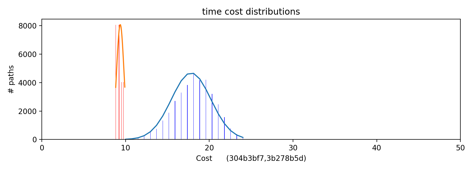
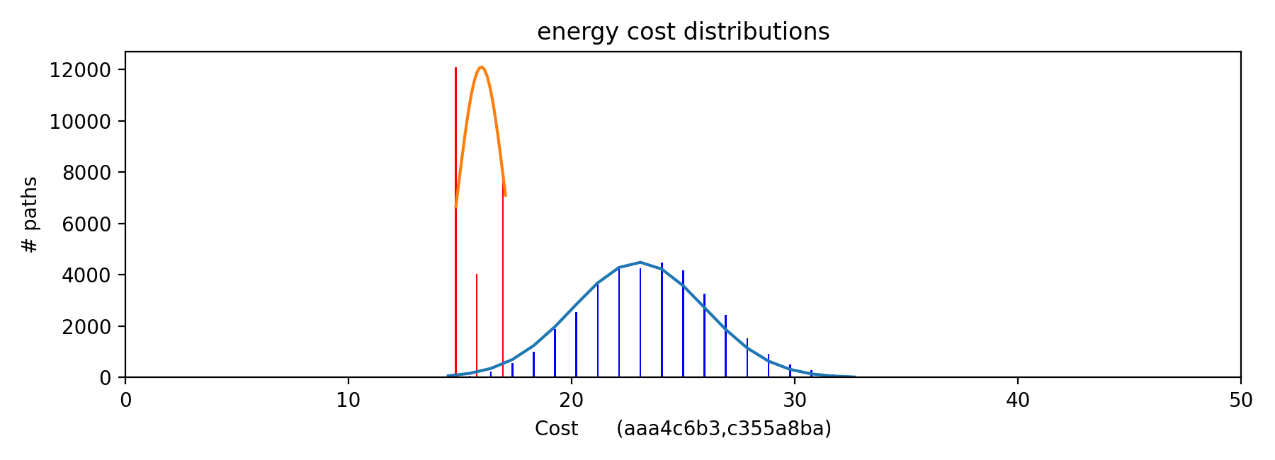
Figure 2: Comparing distributions of 10% heuristic (nearest-neighbor) paths (red) with 10% random search (blue, all 9 starting points) through the 2-D grid ($N=3$) by total time (Top) and total path energy use (Bottom).

III-A2 Random Grid

We generated a grid of 9 random points (uniform $[-1,1]$) and ran both NN and sampled searches. Suboptimal paths on the random grid are shown in Figure 3. Best time and energy costs for the NN searches were 7.6 and 8.5 respectively. The corresponding global optimal trajectories are given in Figure 3. The trajectories appear different and their time and energy costs were lower: 6.1 and 7.0 respectively.

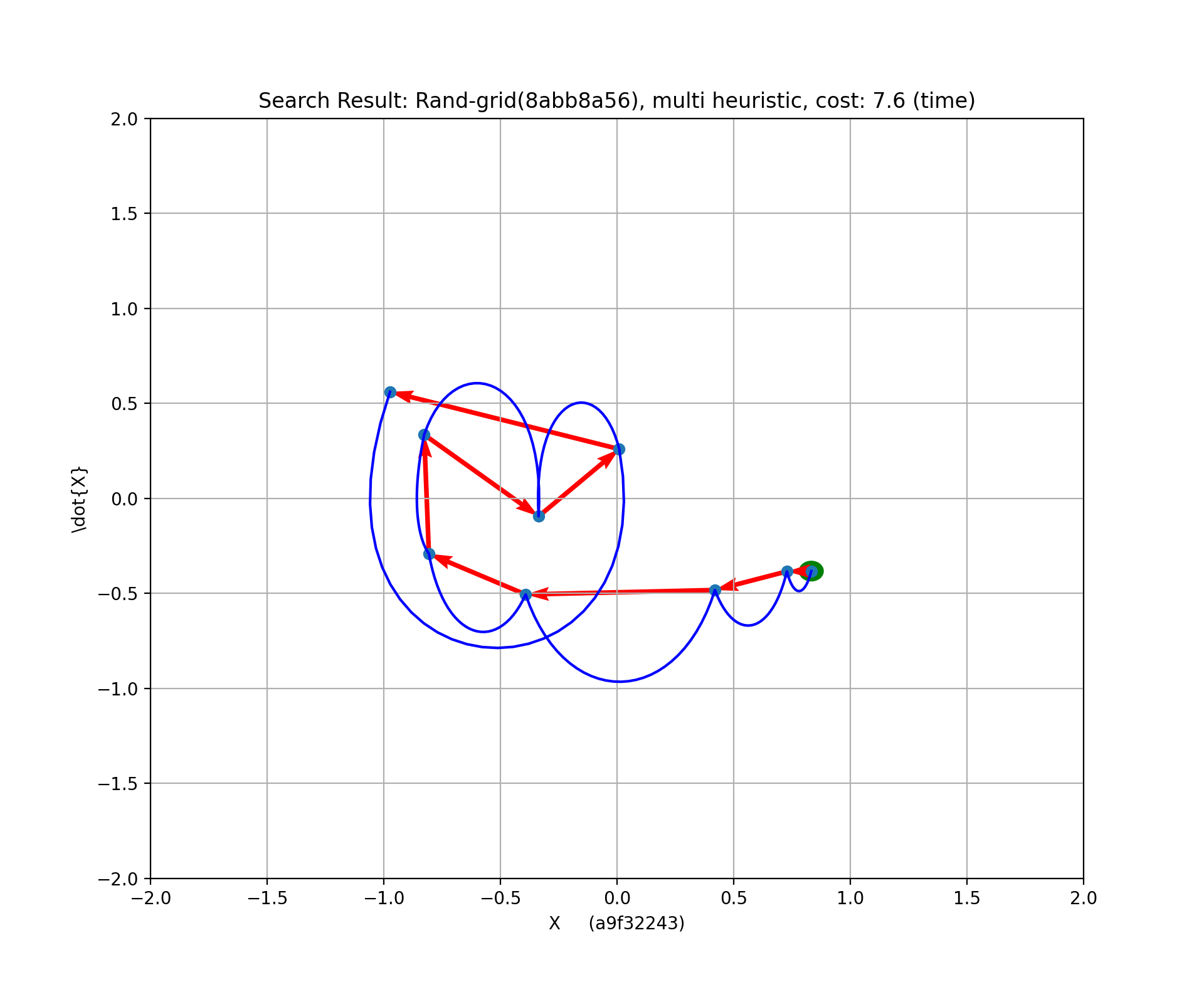
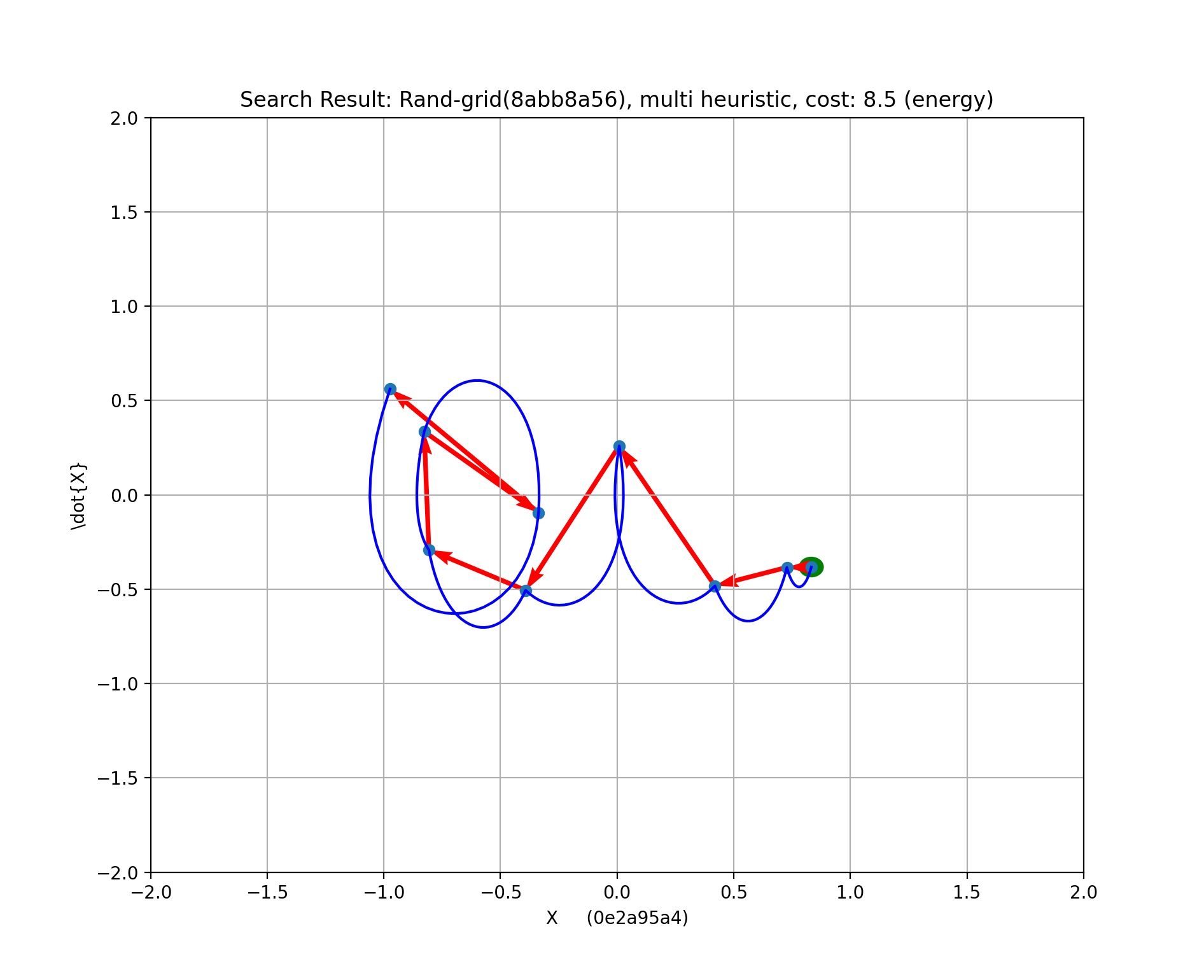
Figure 3: 4 NN searches at each of 9 starting points in a 9-point random grid produced these paths. Path time cost (Top) and energy cost (Bottom). Grid points used (8abb9a56).

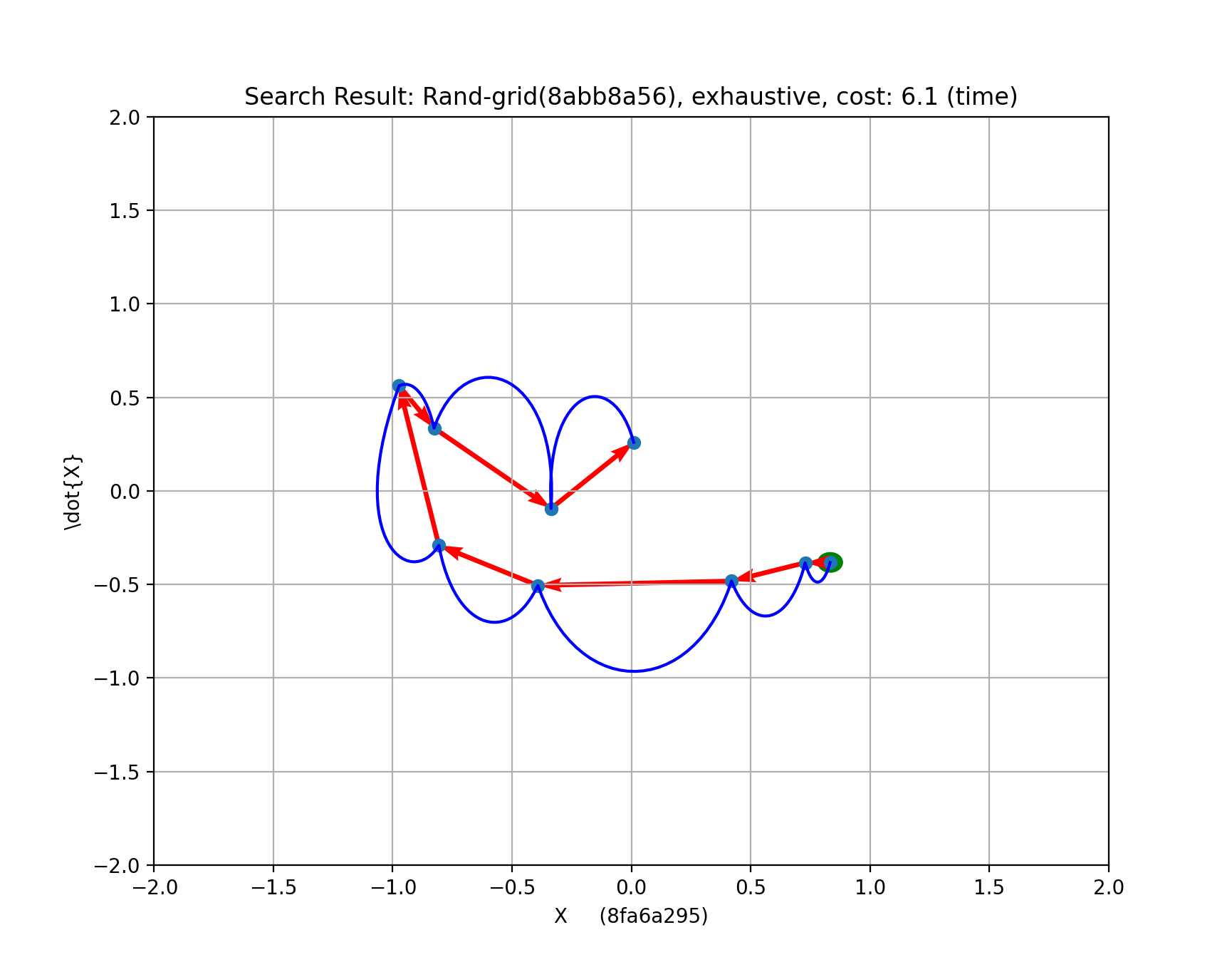
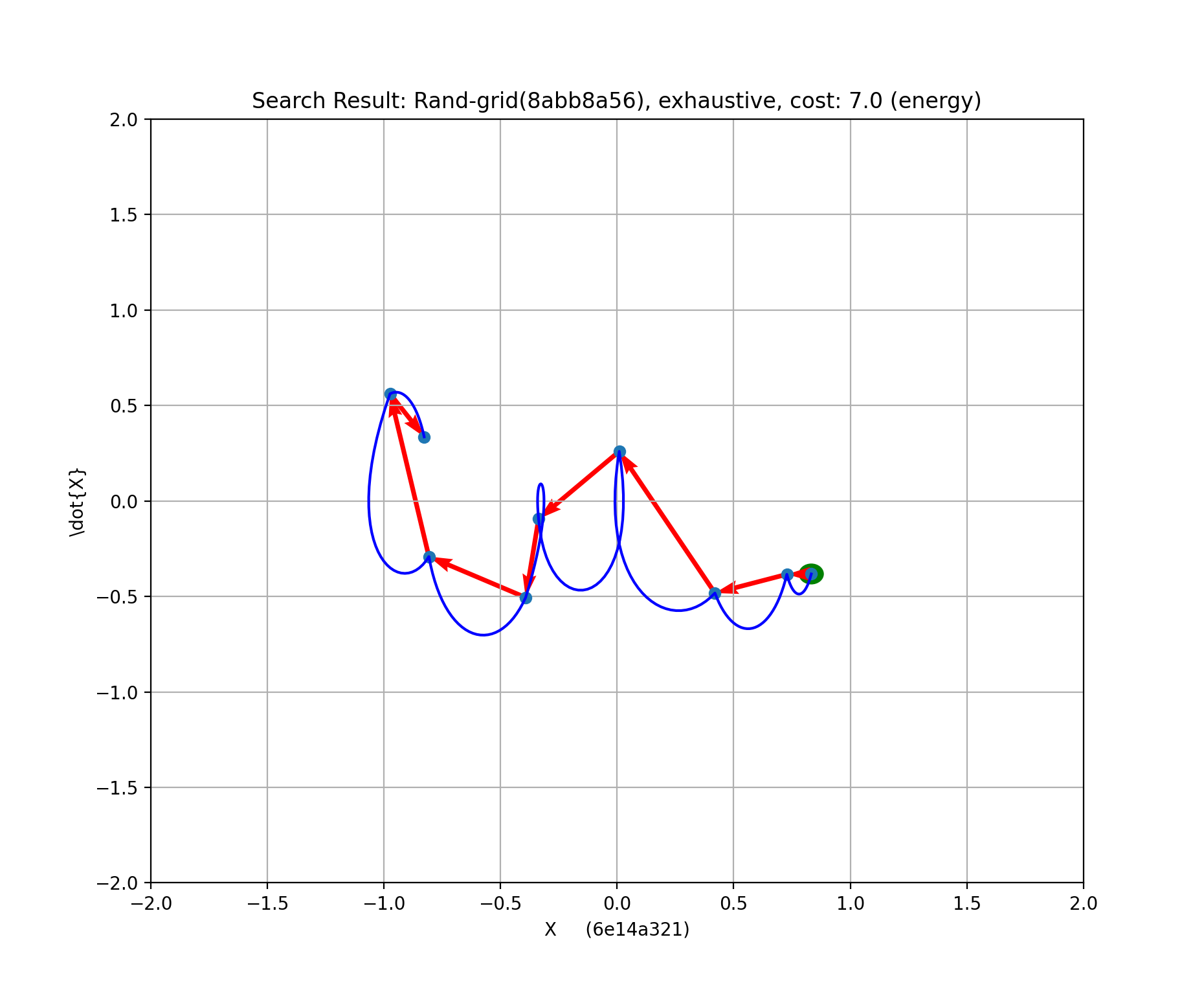
Figure 4: Globally optimum paths on the same random 9 point grid as Figure 3, resulting from exhaustive search. Minimum time cost path (Top) and minimum energy cost path (Bottom). Grid points used (8abb9a56).

III-B 2D, $N=4$

III-B1 Rectangular Grid

As computed above, exhaustive search for a global optimum with 2D, $N=4$ is not feasible. Instead we compared 1 million NN searches vs. 1 million randomly sampled paths.

We generated one million random trajectories by shuffling the integers 0…15 and evaluated their path costs with both time and energy criteria on the rectangular grid. The distributions of cost (Figure 5) are very close to Gaussian. An apparent shift between the Gaussian curve and the sampling bins in this figure is an artifact of the bin plotting. This was confirmed by generating 1M samples of synthetic data with a known mean and observing a similar plot.

III-B2 Normality

A Quantile-Quantile plot of 1M samples of time cost from Figure 5 (Figure 9) shows very close correspondence between the normalized cost data with the normal distribution, $N(0,1)$. Long duration outliers for the time cost are sparse compared to Normal.

For evaluation of search results, the lower tail (negative quantiles) is of most interest. For time cost, the QQ plot extends below the $y=x$ line, indicating that lower outliers are even rarer in the large sample data than they are in the Normal distribution. For energy cost, the situation is reversed, lower outliers are somewhat more common in the large sample data than expected from the Normal distribution.

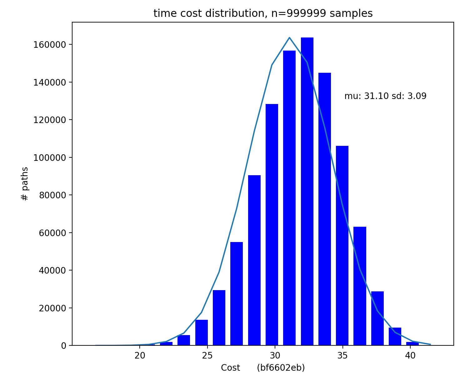
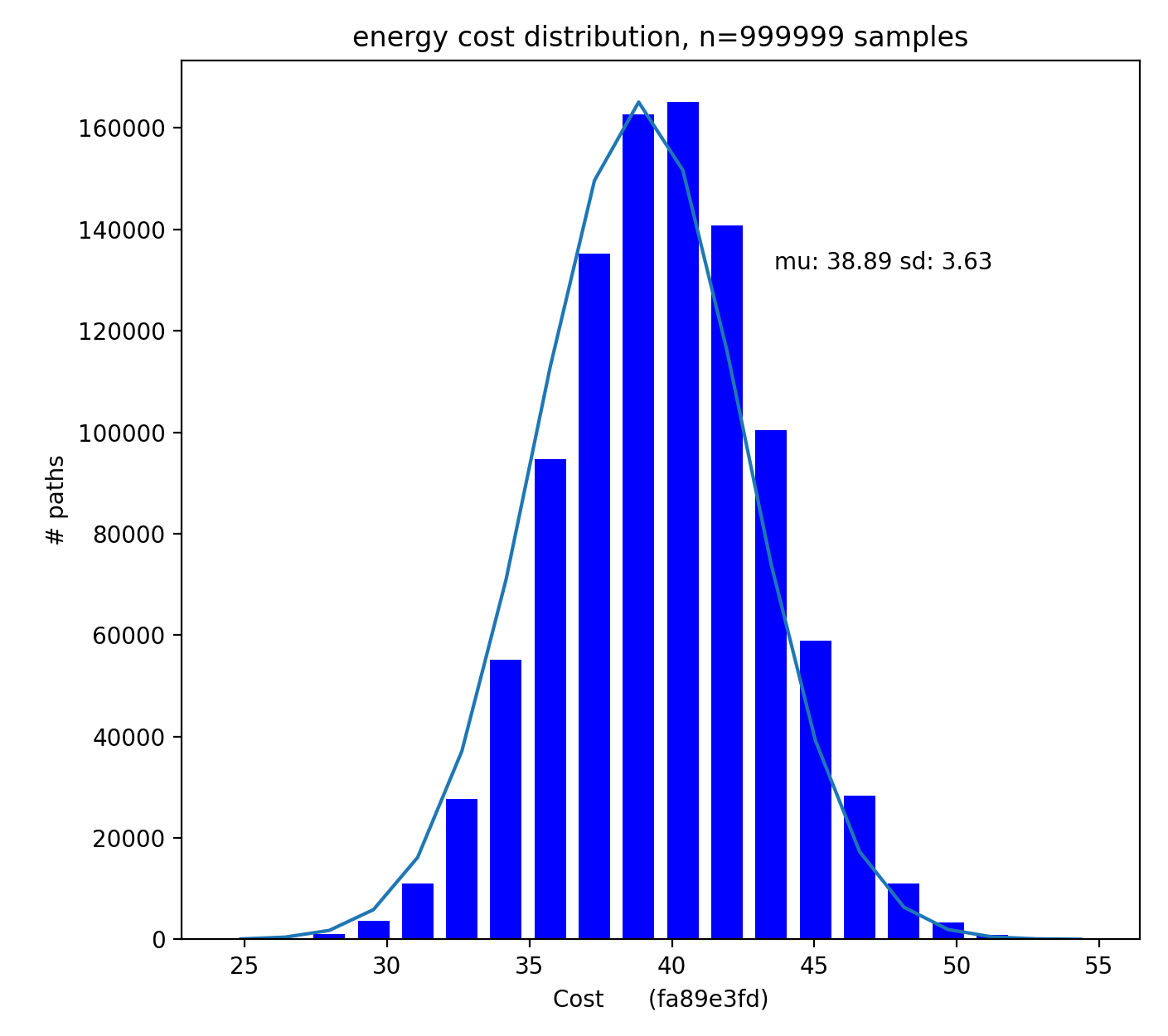
Figure 5: Distribution of one million randomly generated paths through the 2-D phase space (rectangular grid, $N=4$) by total time (Top) and total path energy use (Bottom).

It is noteworthy that the minimum time cost of the 1M sample trajectories (Figure 5) was approximately 16.1 which is quite far out on the left tail of the sample’s distribution. For this particular sample of one million paths, the best time is $4.85\sigma$ below the mean. The minimum energy cost from the sample trajectories was 23.1 which is $4.4\sigma$ below the mean. We compare these outliers discovered by random searching to the NN results in Section VI below.

III-C Random Grid

We repeated the computations of Section III-A1 with a 2D random grid of 16 points ($N=4$).

First we illustrate the best trajectories found with 50,000 randomly sampled trajectories to the best trajectories with 50,000 Multi-Heuristic searches (Figure 6). Recall that we could not find the global optimum for the 2D, $N=4$ grid due to extremely long required computation time. The more optimal paths (lower row of Figure 6) are simpler and pursue clockwise trips through the points. Costs for the trajectories illustrated were substantially lower than the best random sampled trajectories (time: 9.2 vs. 15.0, energy, 12.0 vs. 18.3). These overall effects were similar to the regular grid (Figure 1).

(a) Suboptimal: Time Cost

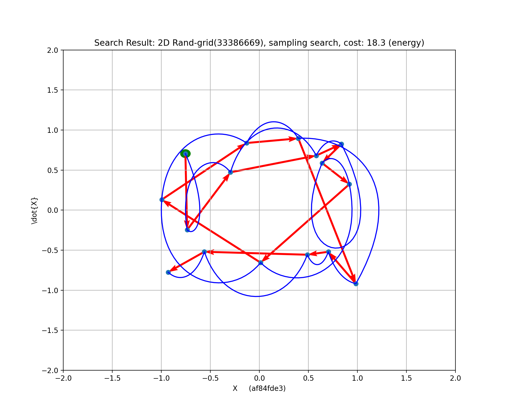
(b) Suboptimal: Energy Cost

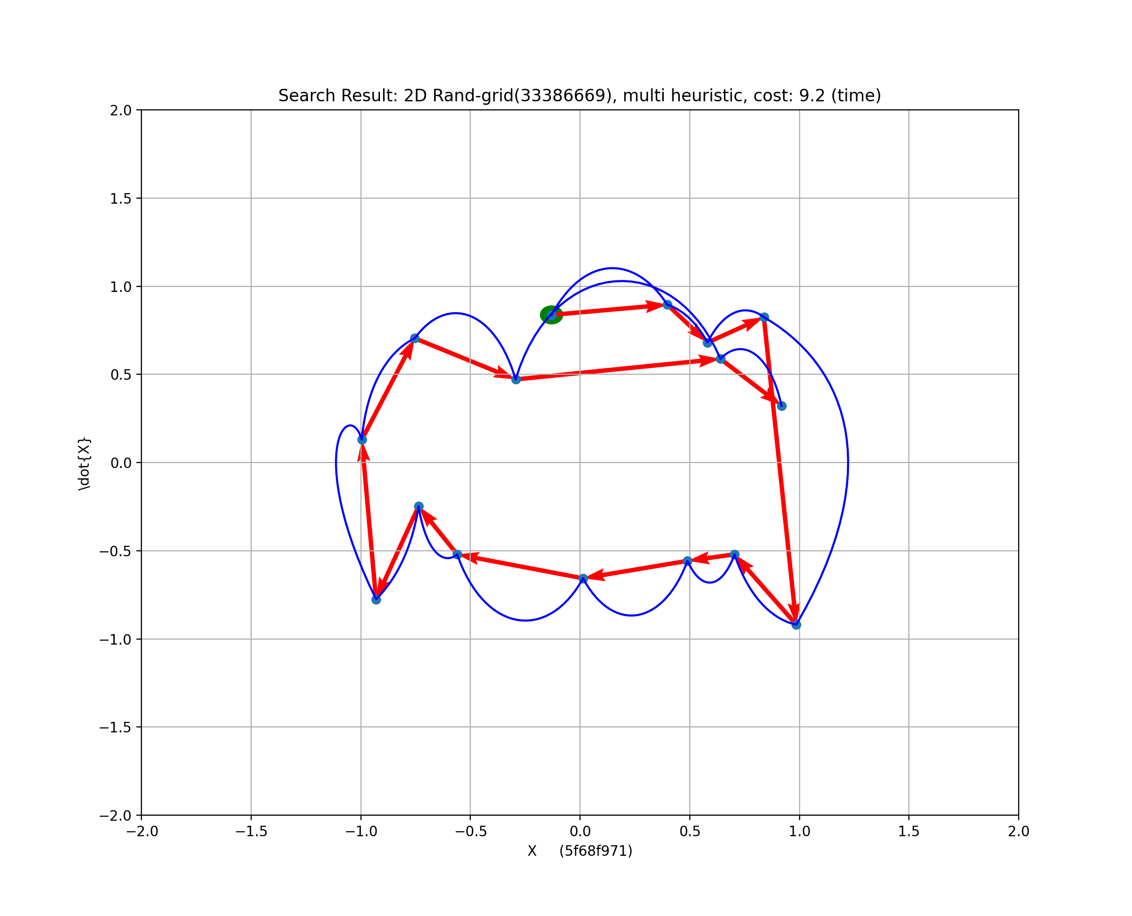
(c) Globally optimal: Time Cost

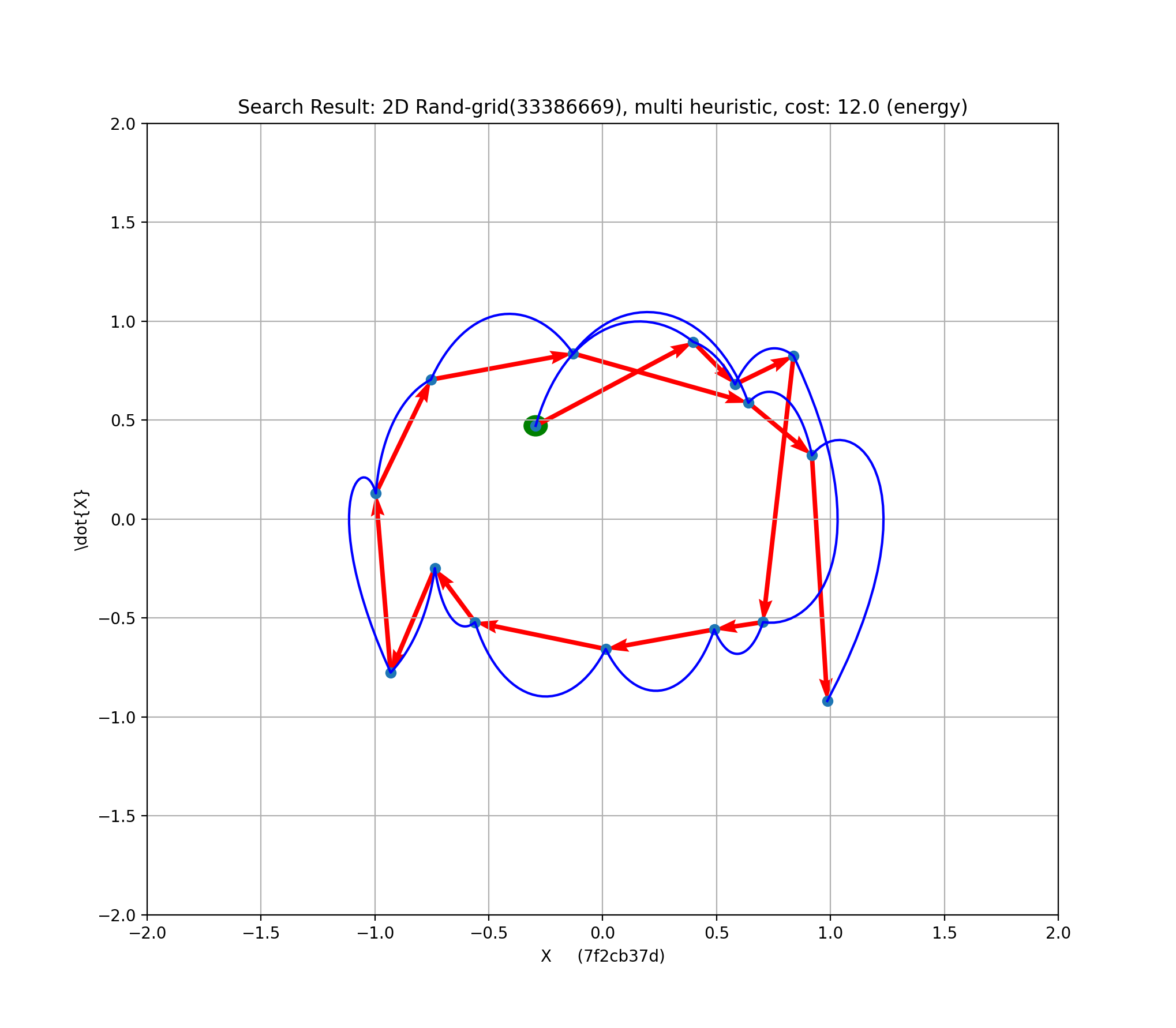
(d) Globally optimal: Energy Cost

Figure 6: 2D, $N=4$ random grid. Best paths from 50,000 random sample paths: (a) total time (b) energy use. Best paths from 50,000 NN searches (c, time, d, energy). (random grid: 33386669).

Comparing the NN cost distributions with the sampled distributions for the random grid (Figure 7) shows little or no overlap between the distributions, and the NN distribution (red), while still non-Gaussian, is becoming closer.

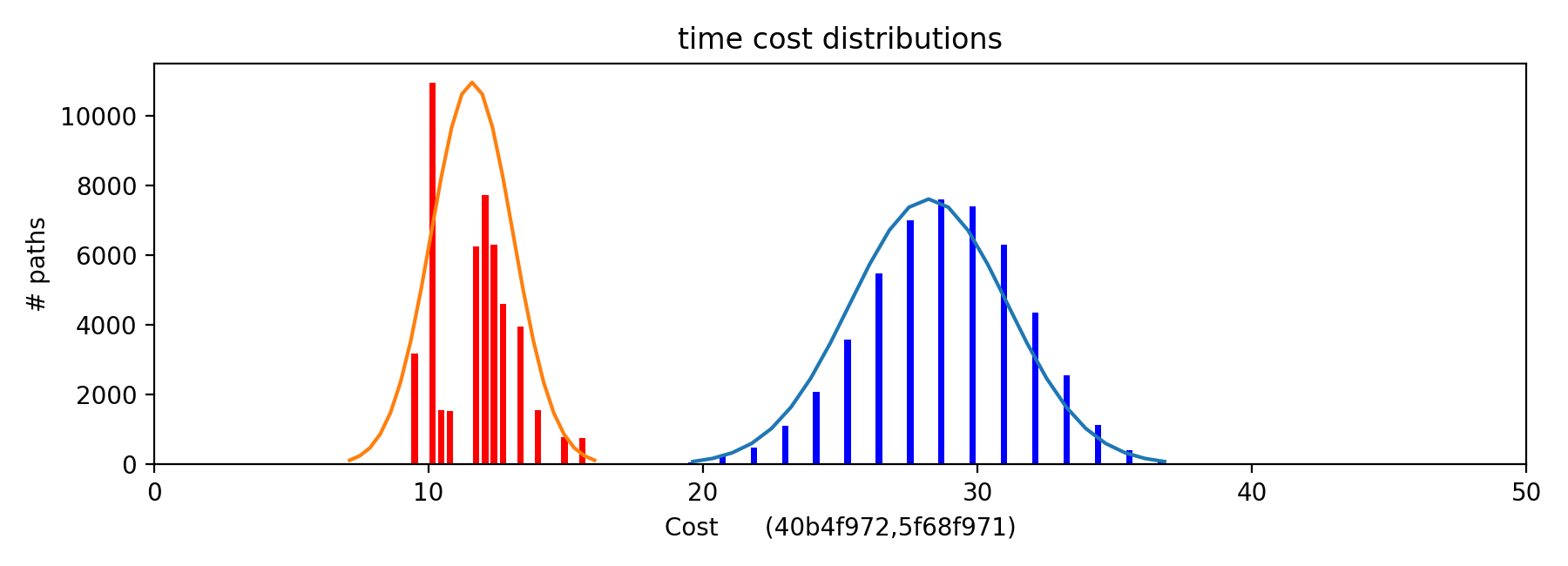
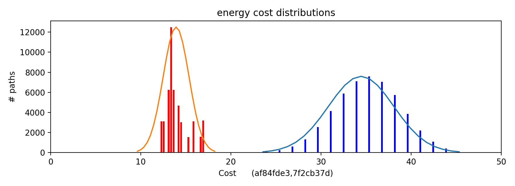
Figure 7: Comparing distributions of 50,000 nearest-neighbor heuristic (NN) paths (red) with 50,000 random paths (all 16 starting points) through the 2-D grid ($N=4$) by total time (Top) and total path energy use (Bottom).(random grid: 33386669).

We again assessed the degree that 1M samples of trajectories on the 2D, $N=4$ random grid fit a normal distribution using the histograms (Figure 8 and the quantile-quantile plot (Figure 10). The substitution of a random grid for the rectangular grid seems to improve the closeness of fit to a Gaussian, particularly in the important lower tail (compare Figure 10 with Figure 9).

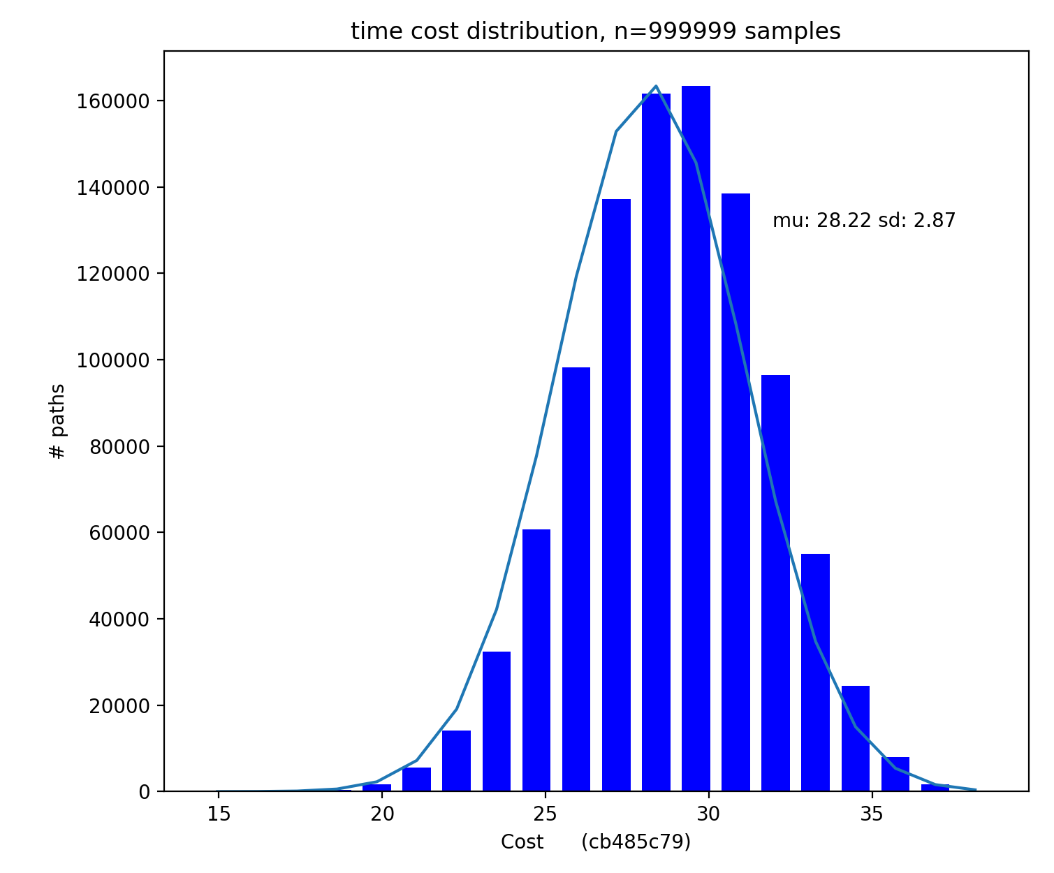
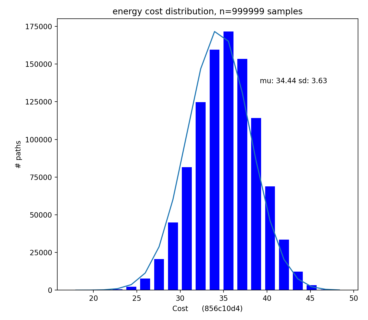
Figure 8: Distribution of one million randomly generated paths through a 2-D, $N=4$ random grid phase space by total time (Top) and total path energy use (Bottom). (random grid ID: 33386669).

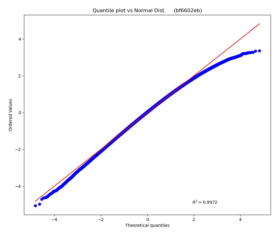
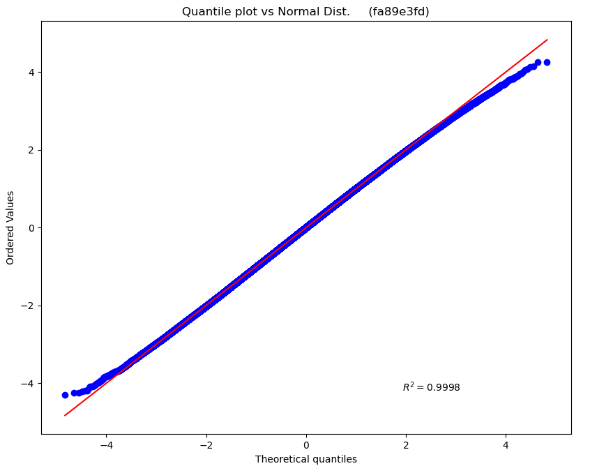
Figure 9: Quantile plots of costs from searching 1M points 2D, 4x4 Rectangular grid (Fig.5) compared with normal distribution (after normalization to mean and standard deviation). Time cost (Top), energy cost (Bottom).

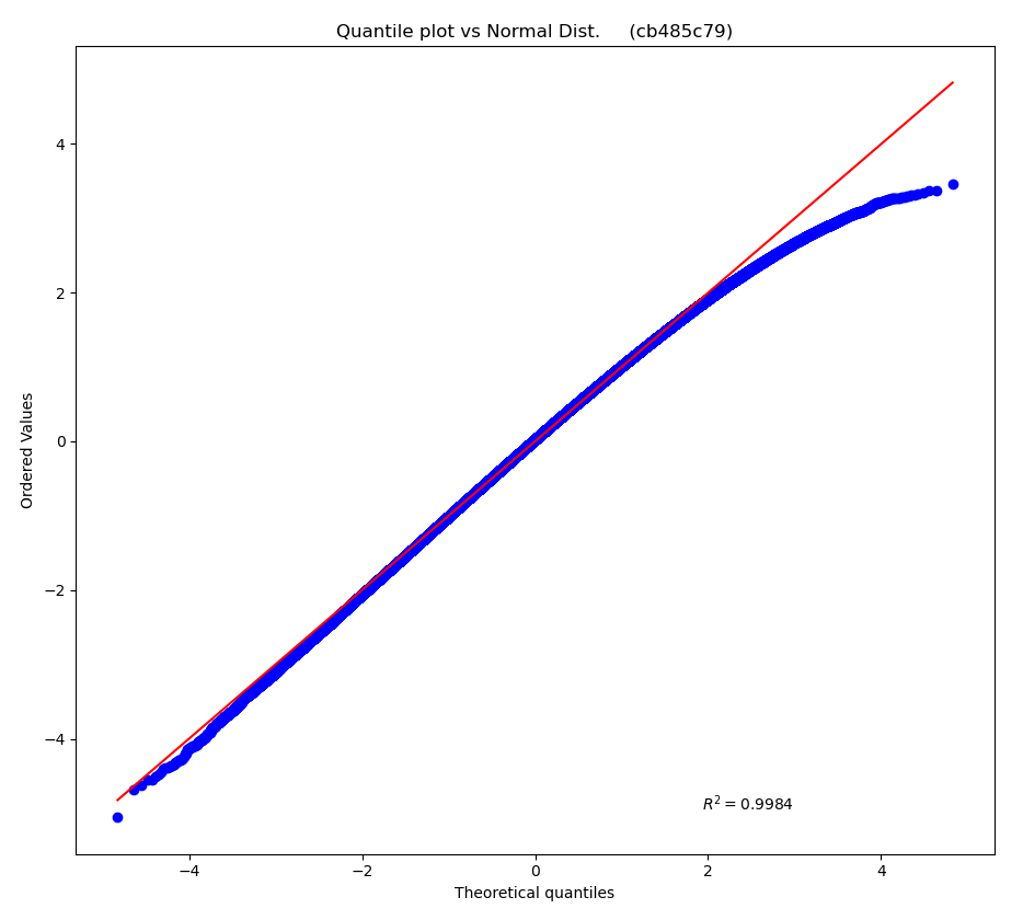
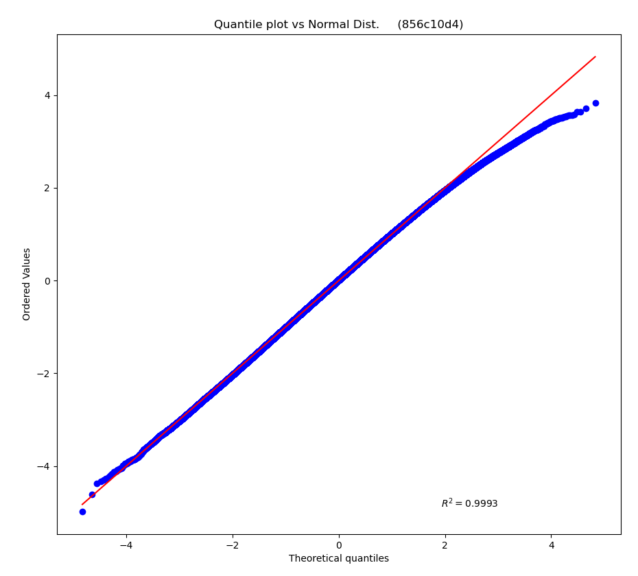
Figure 10: Costs from 1M searches of 2D, 16, Random grid (Fig. 8)/ compared with normal distribution (after normalization to mean and standard deviation). Notably, the negative tail is closer to a perfect normal distribution with the random grid. Time cost (Top), energy cost (Bottom). (random grid: 33386669)

III-D 6D

We now explore the 6D space arising from considering the $X,Y,Z$ positions in a 3D work volume crossed with the end-effector velocities, $\dot{X},\dot{Y},\dot{Z}$.

III-D1 Rectangular Grid

We ran 10,000 NN searches in the 6D, 4x4 rectangular grid, and compared them to a sample of 10,000 random paths (Figure 13). Cost reduction was dramatic for both time and energy costs. However, each 6D, $N=4$ NN search took about 1000 times as much computation time as evaluating the cost of a random path. See Section VI for consideration of this tradeoff.

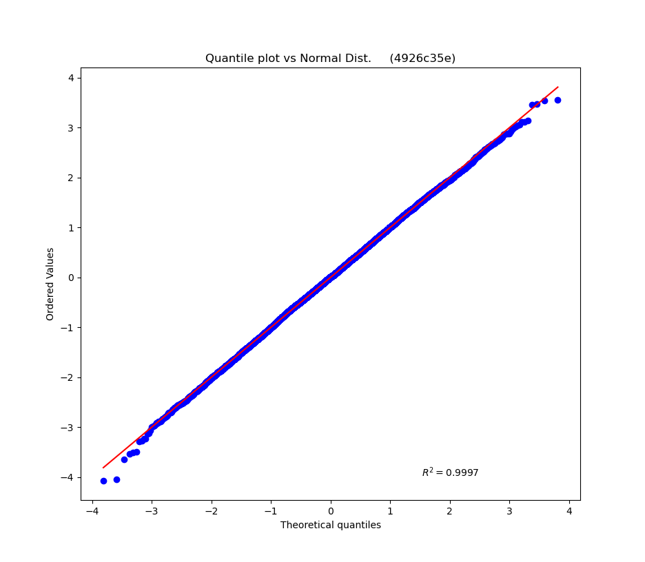
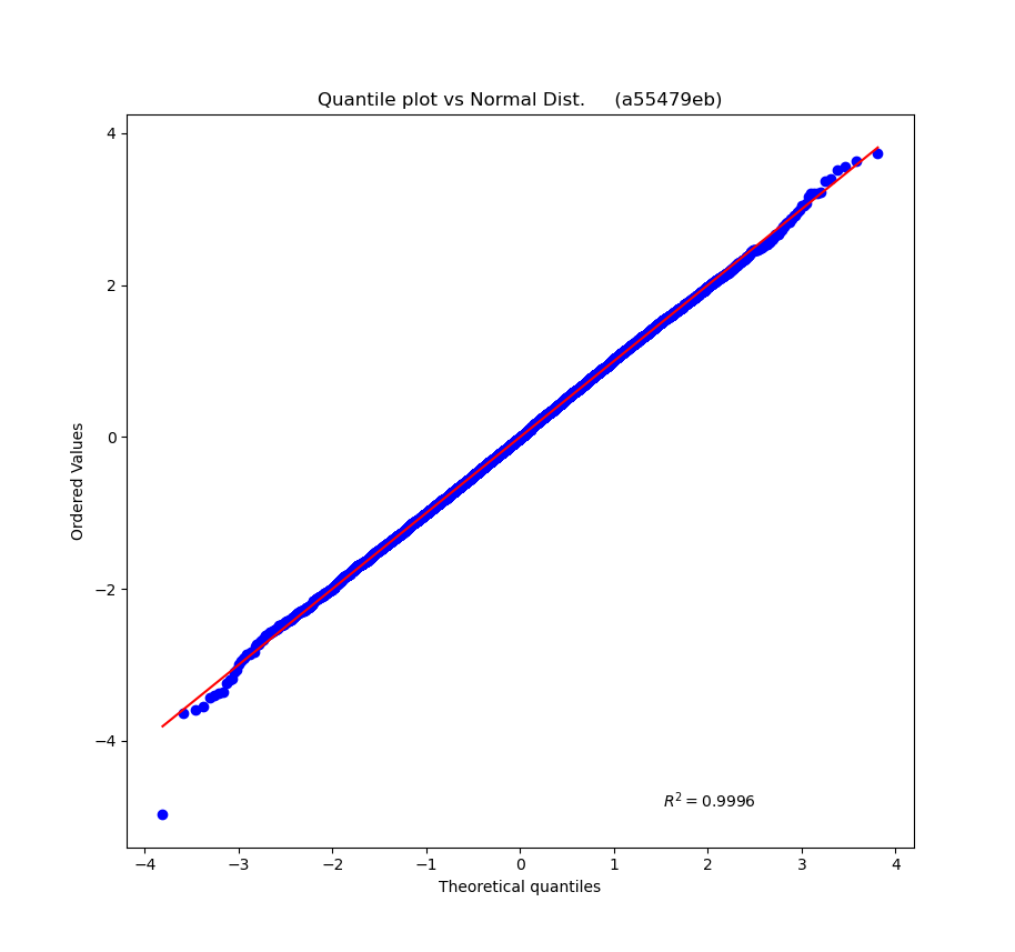
Figure 11: Normality with the 6Dx4x4 Rectangular grid. Quantile plots of 10,000 random trajectories from Figure 13 (blue curve) compared with normal distribution (after normalization to mean and standard deviation). Time cost (Top), energy cost (Bottom). except for a very low cost outlier for Energy cost.

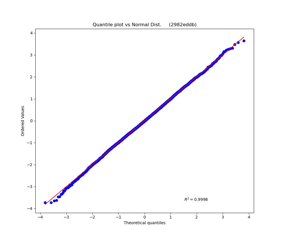
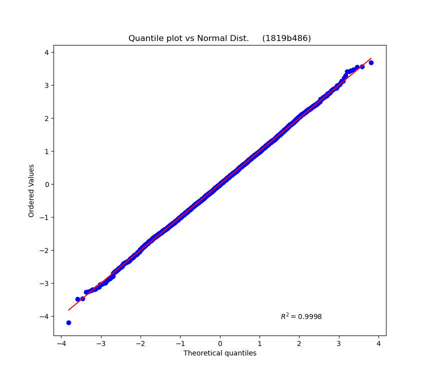
Figure 12: Normality with the 6Dx16 Random grid. Quantile plots of 10,000 random trajectories from Figure 14 (blue curve) compared with normal distribution (after normalization to mean and standard deviation). Notably, the negative tail is closer to a perfect normal distribution with the random grid (compare with Fig. 13). Time cost (Top), energy cost (Bottom). (random grid: 165732fc)

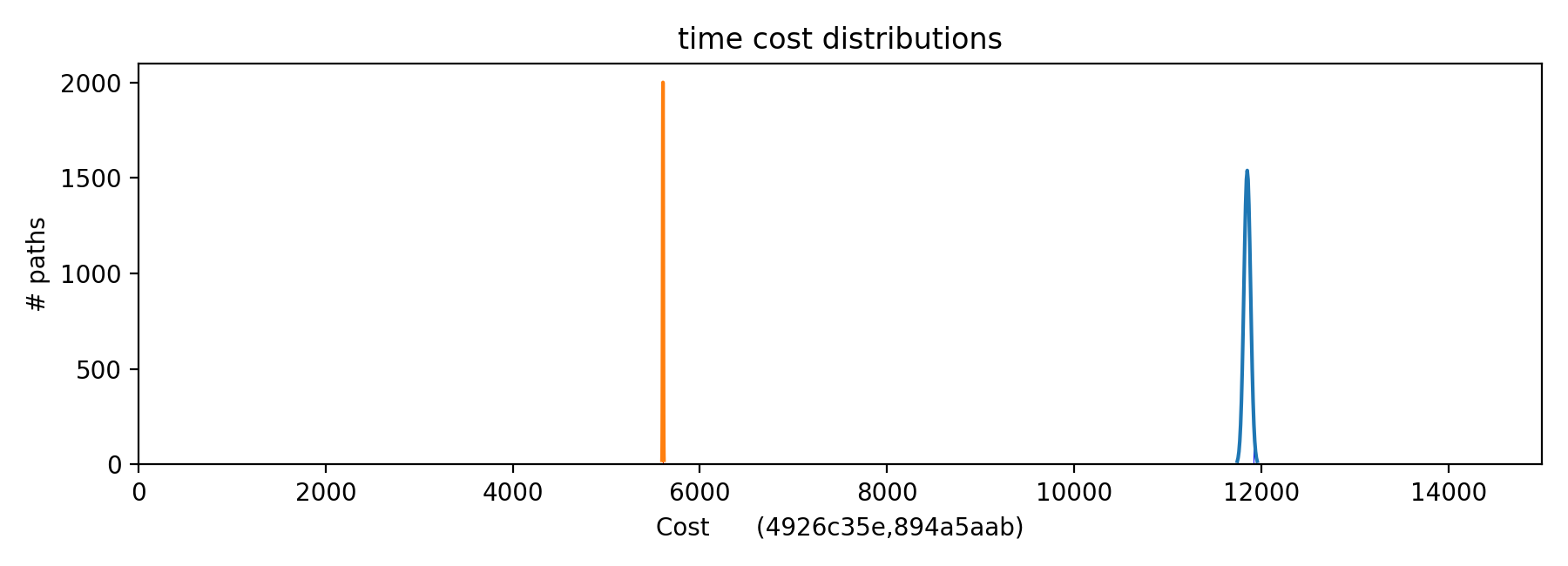
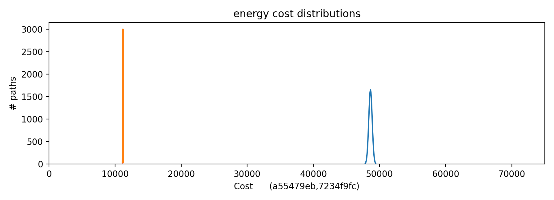
Figure 13: Distributions for time cost (Top) and energy cost (Bottom) of the 6D 4x4 rectangular grid. Note scale change on Energy cost graph. 10,000 random samples (Blue) and 10 nearest neighbor heuristic (NN) searches (Red). Magnitude of NN search result scaled by area to visually match random samples.

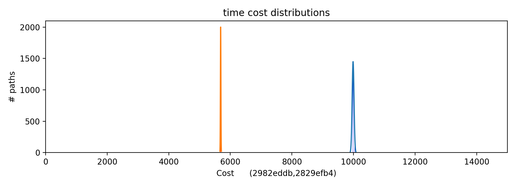
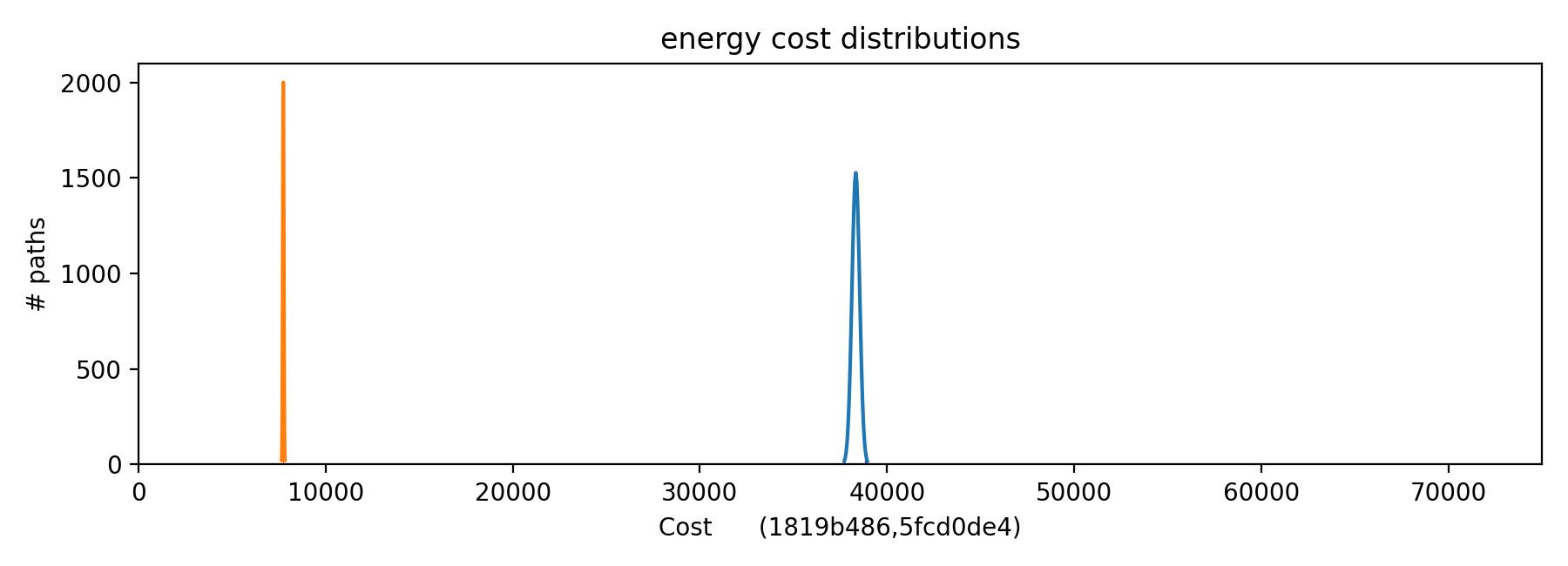
Figure 14: Cost comparisons with a 6D, $N=4$, random instead of rectangular grid for time cost (Top) and energy cost (Bottom). Random samples (Blue) and NN searches (Red). (points dataset 165732fc).

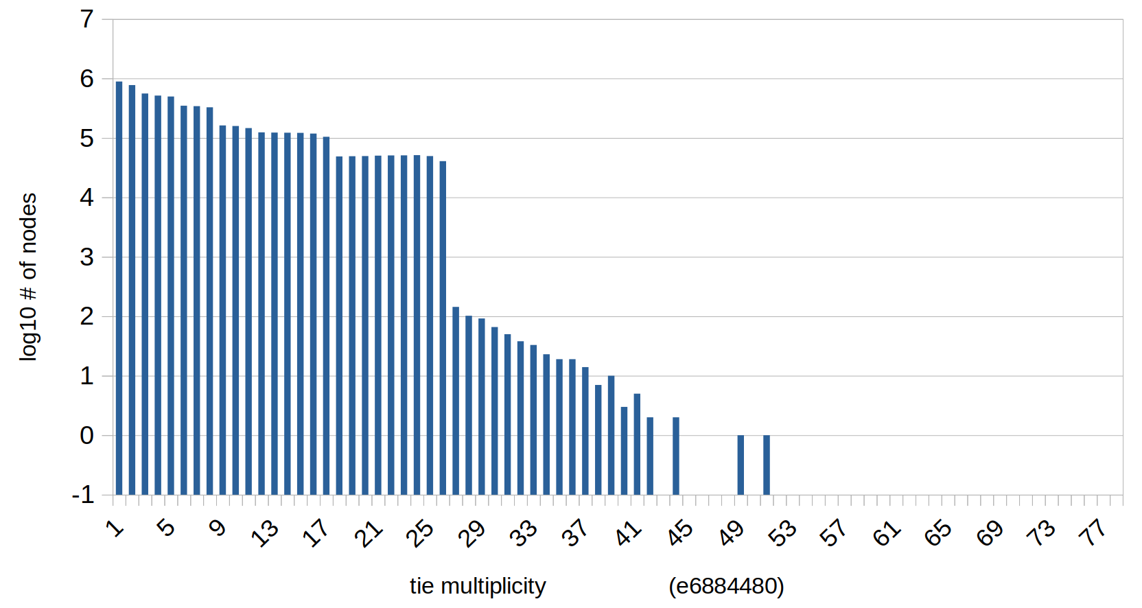
(a) Rectangular Grid: Time Cost

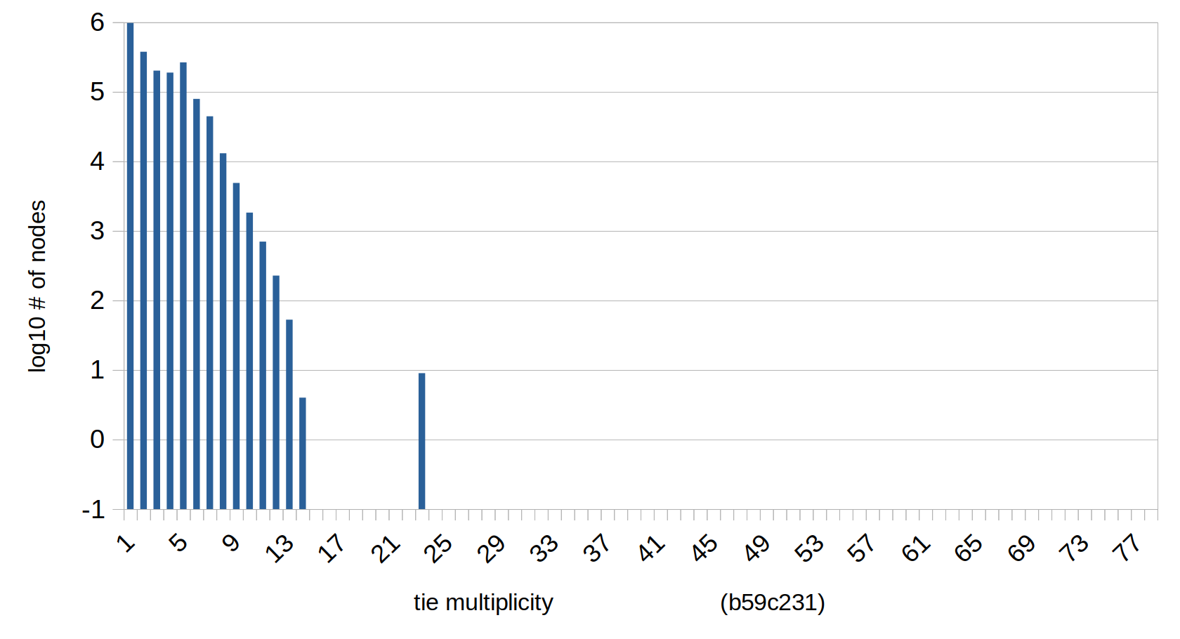
(b) Rectangular Grid: Energy Cost

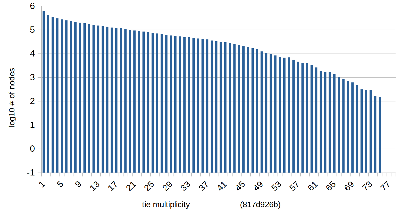
(c) Random Grid: Time Cost

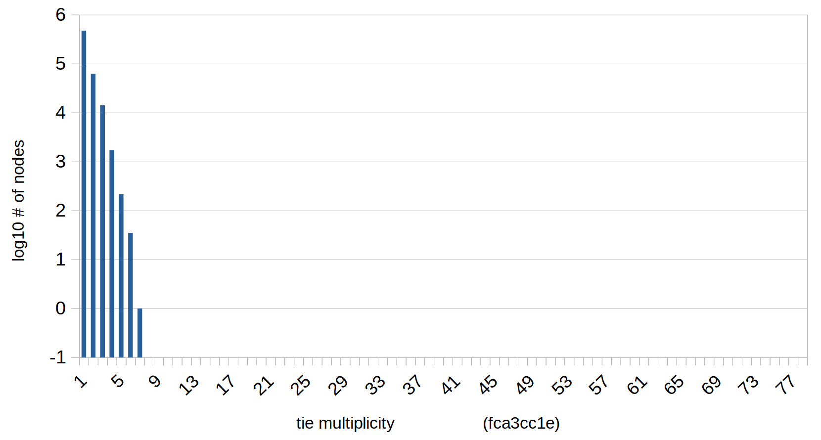
(d) Random Grid: Energy Cost

Figure 15: Distribution of the log number of ties during 10,000 NN heuristic searches 6D, $N=3$ space ( 14 searches per starting point, random point set 73d954cc). For Time cost on random grid (c), the apparent truncation of the distribution at about 76 branches is in the data itself and not due to plotting axis choice.

III-D2 Random Grid

As with the 2D random grid, 6D points were generated at random from a uniform distribution such that for the six dimensions, each coordinate was an independent random variable between $-1$ and $1$.

With all points defined randomly, we ran 10 NN searches for comparison with 10,000 random sampled paths using both the time and energy costs. Execution time for these two computations was about the same as for the rectangular grid (15-20 min.).

Cost performance on the random points

A sample of random paths had lower time costs with randomized points than with the grid (compare Time Cost, Figure13 and 14).

Overall, for 6D, 4x4, costs were substantially similar for both rectangular and random grids.

III-D3 6D Normality

Rectangular Grid: We analyzed the normality of the costs computed from 10,000 randomly sampled trajectories in the 6D 4x4 rectangular grid (Figure ) using the same Q-Q Plot methodology of Figure 9 indicating very Gaussian behavior of costs in the higher dimensional space (Figure 11).

Random Grid: We also analyzed the normality of the costs computed from 10,000 randomly sampled trajectories in the 6D 4x4 random grid (Figure ) which was also highly Gaussian (Figure 12).

III-D4 Ties

Ties (instances where multiple branches from a node have about the same cost) are an interesting feature that seems to be less frequently explored in the literature. Our NN searches of the phase space grids revealed that tie situations are very common for both rectangular and random grids (Figure 15). Prevalence of tied nodes may suggest a large space for additional heuristic improvements in the neighborhood of our paths discovered by the NN heuristic with random tie breaking.

As might be expected, the tie distribution curve is smoother for the random grid and has more discrete features for the rectangular grid. However for the time cost on the random grid, the smooth curve is abruptly truncated in the search data at a maximum tie multiplicity of 76 (i.e. 76 branches with equal cost). It may be surprising that so many ties were found in the random grid. We used a 2% threshold for determining equal cost so this curve may be smaller if a tighter tolerance were used.

IV Conclusions and Discussion

This study has explored ways to most efficiently search a phase space of up to 6 dimensions. We compared nearest-neighbor (NN) searching and random sampling, first on a 2D phase space in which it was feasible to find the global optimum for comparison and then on the 6D space with up to 4 points per axis ($N=4$).

The motivation for this study is efficient collection of motion data over the position and velocity workspace (phase space) of a physical robot for training machine learning algorithms. Efficient search of this space is important for proper coverage of robot operating conditions, feasible training time, and avoidance of over-fitting.

Computation cost for optimal paths grew extraordinarily rapidly as the space dimension approached practical applications. However, when equal computation time is applied to NN search and random sampling there is a vanishingly small probability that the random samples contain a result as good as the NN search. This is perhaps non-obvious since there is evidence [12] that NN algorithms can produce bad results in some TSP problems.

The distribution of costs from random sampling as well as from large numbers of NN searches was very close to Gaussian. This was expected from the literature [13] and it allows estimates of the likelihood that good results could be obtained by NN search results (compared to large random samples). However a limitation of this analysis is that, for the rectangular grids, the quantile-quantile plots from 1 million samples(Figure 9) have inflections in their negative extremes which may invalidate the use of $Z$ statistics.

In future work, we intend to apply these algorithms to programming actual robot motion for efficiently collecting mechanical accuracy training data with sufficient ability to generalize throughout the phase space.

V Appendix: Notation and Basics

V-A Notation

The goal is to search a grid of points in the space consisting of points $P_{i}=\{X_{i},V_{i}\}=\{x,y,z,\dot{x},\dot{y},\dot{z}\}$ within bounds:

$$-1<\{x,y,z,\dot{x},\dot{y},\dot{z}\}<1$$

We wish to visit all the points with as low a cost as possible. We will set up a grid with $N$ points per axis, for a total of $6^{N}$ points or a set of $6^{N}$ random points .

A trajectory, $T_{ij}$ between two points in this space, $T(P_{i},P_{j})$, is a route through the space from $P_{i}$ to $P_{i+1}$ with the properties

$$\Delta X(T_{ij})=\frac{X_{i+1}-X_{i}}{\Delta t}$$ (1)

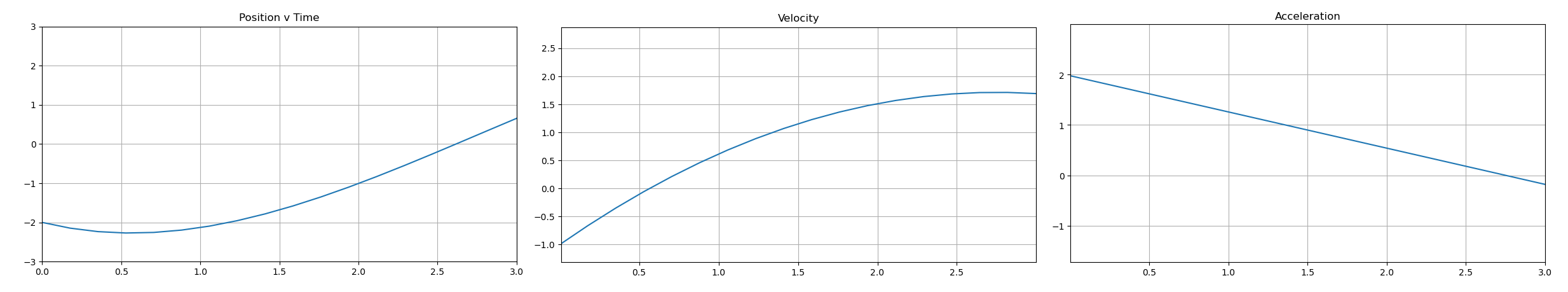
Figure 16: A trajectory between two example points in 2D phase space computed by the 3rd order polynomial.

V-B Trajectories between points

A Trajectory, $T_{ij}$ connects point $P_{i}$ to point $P_{j}$ in phase space with a time function $x(t),0<t<\Delta t$. To meet the constraints

$$x(0)=X_{i},\;x(\Delta t)=X_{j},\;\dot{x}(0)=V_{i},\;\dot{x}(\Delta t)=V_{j}$$ (2)

we can use a 3rd order polynomial having four unknown constants:

$$x(t) =a_{0}+a_{1}t+a_{2}t^{2}+a_{3}t^{3}$$ (3)

$$v(t) =\hskip 19.91692pta_{1}+2a_{2}t+3a_{3}t^{2}$$

$$a(t) =\hskip 45.5244pt2a_{2}+6a_{3}t$$

A typical trajectory of this type, computed for

$$x(0)=-2,\;v(0)=-1,\qquad x(\Delta t)=1.5,\;v(\Delta t)=1.5$$ (4)

is given in Figure 16.

The constants are solved as follows:

$$a_{0}=x(0),a_{1}=v(0)$$ (5)

defining some intermediate terms:

$$\Delta x=x(\Delta t)-x(0)\qquad\Delta v=v(\Delta t)-v(0)$$ (6)

$$b0=\Delta t\qquad b1={\Delta t}^{2}\qquad b2={\Delta t}^{3}$$ (7)

$$b3=2\Delta t\qquad b4=3{\Delta t}^{2}$$ (8)

then

$$a_{3}=\frac{b1\Delta v-b3(\Delta x-v(0)b0)}{b1b4-b2b3}$$ (9)

$$a_{2}=\frac{\Delta x-v(0)b0-a_{3}b2}{b1}$$ (10)

Our goal is to find a minimum cost trajectory satisfying eqn (2) and with the form of eqn (3). Then we can define the cost of each trajectory between two phase-space points at least two ways:

V-B1 Energy Cost

We assume that energy of a trajectory is

$$C_{e}(T_{ij})=\int_{0}^{\Delta t}a(t)^{2}dt$$ (11)

this can be solved using (3) as

$$C_{e}(T_{ij})=4a_{2}(\Delta t)+12a_{2}a_{3}(\Delta t)^{2}+12a_{3}^{2}(\Delta t)^{3}$$ (12)

V-B2 Duration Cost

The time cost, $C_{t}$ is

$$C_{t}(T_{ij})=\Delta t$$ (13)

V-B3 Acceleration Constraint

To assure that our trajectories, $x(t),v(t),a(t)$ are feasible for a real robot manipulator, we will constrain

$$|a(t)|<a_{max}\qquad 0<t<\Delta t$$ (14)

Furthermore we wish to complete the trajectory as fast as feasible, so we will set this constraint to equality:

$$\max(|(a(t)|)=a_{max}$$ (15)

From eqn (3) we know that acceleration is linear with time for all solutions, thus we have:

$$\max(|a(t)|)=\max(|a(0)|,|a(\Delta t)|)$$ (16)

We iteratively minimize $\Delta t$ for each trajectory until eqn (15) is satisfied within about 2%.

V-C Path Cost

A path, $\mathbf{P}$, is a sequence of trajectories (indexed by $k$), $T_{ijk}$, connecting $P_{i}$ to $P_{j}$ such that the trajectories are connected, e.g.

$$P_{j}(T_{ijk})=P_{i}(T_{ijk+1})$$ (17)

the points $P_{i}$ covering the entire grid. Let $C_{k}=C_{x}(T_{ijk})$ be the cost of the $k^{th}$ trajectory in the path, $\mathbf{P}$. The time cost of visiting every point in the path is

$$C_{T}=\Sigma_{k}C_{k}\qquad 0\leq i<N^{m}$$ (18)

For example, the total time cost of path ${P}_{1}$ would be

$$C_{Tp1}=\Sigma_{k}C_{t}(T_{ijk})$$ (19)

where $T_{ijk}$ is the $k^{th}$ trajectory of path ${P}_{1}$.

VI Appendix: Statistical Analysis of NN search vs. random sampling in 6D

In this section we evaluate the likelihood that random sampling, since it is much faster computationally, could in fact produce a result as good as nearest-neighbor heuristic searching if the same computational resources are applied. In higher dimensions we don’t know the global optimum path but NN searching produces very low cost paths compared to random samples. [13] performed a probabilistic analysis of the TSP, but it was limited to symmetric and Euclidean problems.

We use the Z-statistic in three ways to determine how much better the NN search result is than choosing the lowest cost from a large number of random samples. But first, we must equalize the computing resources for a fair comparison. Random sampling is much more efficient than the NN search because random paths are generated by permutations, and we only have to evaluate the sum of all branch costs in the path ($O(n)$, where $n$ is the path length). In contrast, with the NN search, at each node, we have to evaluate the cost of all un-visited branches to get the minimum cost value, and in our case search again to find the set of ’tied’ nodes ($O(n^{2})$).

We experimentally determined that for our 6D problem with grid size 3, 10 NN searches took about the same computation time as did computing the costs of 10,000 random trajectories and selecting the lowest cost path. We are therefore able to compare the two cases statistically.

The first Z-statistic is somewhat traditional. If $\mu_{samp}$ and $\sigma_{samp}$ describe the 10,000 samples, and $\mu_{NN}$ is the mean of a set of NN results, we have

$$Z=\frac{\mu_{NN}-\mu_{samp}}{\sigma_{samp}}$$ (20)

We could also define a similar statistic, $Z^{\prime}$ in terms of the minimum value of the two samples, since they are readily available computationally:

$$Z^{\prime}=\frac{min(NN)-min({sample})}{\sigma_{samp}}$$ (21)

and to evaluate the worst case,

$$Z^{\prime\prime}=\frac{max(NN)-min({sample})}{\sigma_{samp}}$$ (22)

We can view $\{Z,Z^{\prime},Z^{\prime\prime}\}$ as multiples of $\sigma_{samp}$ to judge how “rare” is each NN search result. These Z-scores are all negative for our data since NN searching gives lower cost than 10,000 samples in all experiments.

The probability, $P_{c}$, that a randomly selected path would have lower cost than $Z$, is

$$P_{c}(Z)=1.0-CDF(Z)=1.0-\int_{-\infty}^{Z}N(t)dt$$ (23)

where $N(t)$ is the normal distribution. We can make analogous definitions for the min and max $Z$ scores, $Z^{\prime},Z^{\prime\prime}$.

We consider the case where 10,000 random samples are drawn from a normal distribution. For a given $Z$, what is the probability that a lower value will not turn up in the 10,000 samples? The probability, $P_{h}$, that a single sample path will NOT have lower cost is

$$P_{h}=1.0-P_{c}(Z)$$ (24)

If we draw $n$ times, and the samples are independent, then the probability that a lower value will not be drawn, $P_{hn}$, is

$$P_{hn}=(P_{h})^{n}$$ (25)

Thus, the probability that $n$ random samples WILL include one with a lower Z score is

$$P_{ln}=1.0-P_{hn}=1.0-(P_{h})^{n}=1.0-(1.0-P_{c}(Z))^{n}$$ (26)

Where $P_{ln}$ is the probability of drawing a lower cost sample in $n$ tries.

Using Python3’s scipy.stats package, the most negative integer Z score that gives a non-zero cdf probability is $Z=-8$ which gives $P_{c}(-8)=6.661\times 10^{-16}$. Using this conservative Z value, and $n=10,000$, eqn (26) gives $P_{hn}=6.661\times 10^{-12}$.

Thus the probability that 10,000 random searches would find a result as good as the NN search is on the order of 1 in a trillion, and even lower for Z-scores below -8.

The results (Table I) show this comparison for the rectangular grid (rows 1-4) and three different random grids (rows 5-16). 10 iterations (from different random starting points) are compared with 10,000 random path costs for both Time and Energy. The table shows

• $Z$ and $Z^{\prime}$ statistic values for the NN searches range from $-45\geq Z\geq-74$, dramatically greater than the $Z=-8$ example above.

• $Z^{\prime\prime}$ statistics (not shown in table for reasons of space) were slightly lower than $Z$ and $Z^{\prime}$ and ranged from -40 to -70.

• Computation times are approximately equivalent (31-51sec).

• Results for 3 different random grids were nearly the same (rows 5-16).

We can thus conclude that the NN search is substantially more efficient than sampling. There may be a feasible computation time greater than 1 minute which might do as well as the NN search (which does not seem to improve much with increasing search sizes). But the very large $Z$ scores suggest otherwise.

These results may be affected by the inflections of the Quantile-Quantile plot (Figure 9) but since that plot includes all the data above, the effect should be small and predominantly affect energy cost.

Exp	D	N	Grid	Cost	Srch	N	mu	min	sig	Z	Z’	T(sec)	hash
1	6	3	rect	Time	samp	10,000	2245	2186	16.5			51.0	cbc78246
2	6	3	rect	Energy	samp	10,000	9412	8952	123.0			53.0	5470ef83
3	6	3	rect	Time	NH	10	1019	1013		74.3	71.1	40.0	3a9de6e6
4	6	3	rect	Energy	NH	10	3404	3372		48.8	45.4	38.0	4718555c
5	6	3	rand 73d954cc	Time	samp	10,000	1784	1733	12.7			47.0	cdb3c021
6	6	3	rand 73d954cc	Energy	samp	10,000	6885	6546	88.2			49.0	548ee970
7	6	3	rand 73d954cc	Time	NN	10	1024	1021		59.8	56.1	38.0	dfcc9b7b
8	6	3	rand 73d954cc	Energy	NN	10	1634	1612		59.5	55.9	31.0	c3e8227b
9	6	3	rand 786d6950	Time	samp	10,000	1770	1718	12.6			47.0	1c1c207e
10	6	3	rand 786d6950	Energy	samp	10,000	6819	6504	84.0			47.5	f954b7fd
11	6	3	rand 786d6950	Time	NN	10	1027	1023		59.2	55.3	39.2	54ed4a67
12	6	3	rand 786d6950	Energy	NN	10	1754	1720		60.3	57.0	34.8	a219c0bc
13	6	4	rand 6d5755b7	Time	samp	10,000	1799	1737	12.6			47.2	d98ce58c
14	6	4	rand 6d5755b7	Energy	samp	10,000	6892	6545	86.4			46.0	ded60da5
15	6	4	rand 6d5755b7	Time	NN	10	1031	1028		61.0	56.3	40.0	d48770a4
16	6	4	rand 6d5755b7	Energy	NN	10	1806	1764		58.9	55.3	38.8	e96bd1eb

TABLE I: Computational experiments exploring practicality of NN search results. For both Time and Energy costs, NN searching produces a dramatically better result than the best randomly chosen path if computation time is approximately the same. $Z^{\prime\prime}$ scores (not shown) were 45-70. Hash codes identify pertinent data files.

References

- [1] Mohammad Haghighipanah, Muneaki Miyasaka, and Blake Hannaford. Utilizing elasticity of cable-driven surgical robot to estimate cable tension and external force. IEEE Robotics and Automation Letters, 2(3):1593–1600, 2017.
- [2] Muneaki Miyasaka, Mohammad Haghighipanah, Yangming Li, and Blake Hannaford. Hysteresis model of longitudinally loaded cable for cable driven robots and identification of the parameters. In 2016 IEEE International Conference on Robotics and Automation (ICRA), pages 4051–4057. IEEE, 2016.
- [3] Haonan Peng, Xingjian Yang, Yun-Hsuan Su, and Blake Hannaford. Real-time data driven precision estimator for raven-ii surgical robot end effector position. In 2020 IEEE International Conference on Robotics and Automation (ICRA), pages 350–356. IEEE, 2020.
- [4] Minho Hwang, Brijen Thananjeyan, Samuel Paradis, Daniel Seita, Jeffrey Ichnowski, Danyal Fer, Thomas Low, and Ken Goldberg. Efficiently calibrating cable-driven surgical robots with rgbd fiducial sensing and recurrent neural networks. IEEE Robotics and Automation Letters, 5(4):5937–5944, 2020.
- [5] Jill Cirasella, David S Johnson, Lyle A McGeoch, and Weixiong Zhang. The asymmetric traveling salesman problem: Algorithms, instance generators, and tests. In Workshop on Algorithm Engineering and Experimentation, pages 32–59. Springer, 2001.
- [6] David S Johnson, Gregory Gutin, Lyle A McGeoch, Anders Yeo, Weixiong Zhang, and Alexei Zverovitch. Experimental analysis of heuristics for the atsp. The traveling salesman problem and its variations, pages 445–487, 2007.
- [7] Abraham P Punnen. The traveling salesman problem: Applications, formulations and variations. In The traveling salesman problem and its variations, pages 1–28. Springer, 2007.
- [8] Robert G Bland and David F Shallcross. Large travelling salesman problems arising from experiments in x-ray crystallography: a preliminary report on computation. Operations Research Letters, 8(3):125–128, 1989.
- [9] C Rego and F Glover. The traveling salesman problem and its variations, 2002.
- [10] Aviv Adler. The Traveling Salesman Problem for Systems with Dynamic Constraints. PhD thesis, Massachusetts Institute of Technology, 2023.
- [11] Michael Jünger, Gerhard Reinelt, and Giovanni Rinaldi. The traveling salesman problem. Handbooks in operations research and management science, 7:225–330, 1995.
- [12] Gregory Gutin, Anders Yeo, and Alexey Zverovich. Traveling salesman should not be greedy: domination analysis of greedy-type heuristics for the tsp. Discret. Appl. Math., 117:81–86, 2001.
- [13] Alan M Frieze and Joseph E Yukich. Probabilistic analysis of the tsp. In The traveling salesman problem and its variations, pages 257–307. Springer, 2007.