Continuum And Line Emission From Accretion Shocks at T Tauri Stars I. Correlations With Shock Parameters
Abstract
Fourteen models are calculated with the shock velocity ranging from 200 to 330 km s-1 and pre-shock hydrogen nucleon density ranging from to cm-3. Among them the summed emergent flux of all spectral lines accounts for about 0.1-0.3 of the total veiling flux. The hydrogen Balmer continuum accounts for 0.17-0.1, while a nearly constant fraction close to 0.5 comes from emission produced by the stellar atmosphere. The main results derived from the veiling continuum energy distributions are two strong correlations: 1) the Balmer jump (BJ) increases as , the shock kinetic energy flux, decreases; 2) at a fixed fraction of surface coverage by accretion shocks , the ratio of veiling to photospheric continuum flux at wavelength , decreases as decreases. Using the BJ - and - relations, the observed excess continua of 10 T Tauri stars are modelled. For BP Tau and 3 Orion stars our accretion luminosities are higher than published values by a factor of a few. For the 6 Chamaeleon I stars our observed accretion luminosities are about 27 - 78% higher than corresponding published values. Comparison of model results on the HeI 5876Å flux with observed data indicates that, while those stars with dominant 5876Å narrow components can be readily accounted for by the calculated models, those with much stronger broad components cannot, and suggests that for the latter objects the bulk of their excess continua at 5876Å do not originate from accretion shocks.
1 Introduction
The phenomenon of accretion onto a T Tauri star via infall from a circumstellar disk along magnetic field lines is now well established (Hartmann, Herczeg & Calvet 2016). The key observation pointing to presence of an accretion shock is the continuum excess over the photospheric continuum that is readily detected at UV wavelengths through broadband photometry and at optical wavelengths from the reduction of absorption depths of photospheric lines in comparison with non-accreting weak T Tauri stars (Basri & Batalha 1990). Another observation signalling infall is the presence of red absorptions spanning velocity widths of 100 km s-1 and extending to 300 km s-1 in certain spectral lines. A third observation that also suggests an accretion shock is the presence of prominent narrow components in some spectral lines, notably HeI 5876Å (Beristain, Edwards & Kwan 2001, hereafter BEK01) and CIV 1549Å (Ardila et al. 2013). Magnetic field strengths of several KG inferred from the wavelength separation between right and left circularly polarized components of the HeI 5876Å narrow profile in several T Tauri stars affirm the formation of the narrow component in close proximity to the star (e.g. Johns-Krull et al. 2013). Theoretical calculation of line formation in an accretion shock is still needed, however, to fully verify the origin of the narrow components.
Detailed theoretical modelling of an accretion shock at a T Tauri star was first presented by Calvet & Gullbring (1998). They calculated the radiation spectrum produced by the post-shock gas, using a cooling rate as a function of temperature generated from the work of Raymond & Smith (1977). Half of this radiation spectrum propagates towards the pre-shock zone and, through photoionization, is reprocessed into a continuum spectrum, half of which emerges and forms part of the overall veiling continuum. The other half of this continuum spectrum, together with the remaining half of the above radiation spectrum generated in the post-shock zone, propagates towards the star. Calvet & Gullbring (1998) calculated the emergent continuum spectrum produced by the stellar atmosphere upon absorption of this incident radiation as well as the flux emergent from the stellar interior below. This emergent continuum spectrum forms the remaining part of the veiling continuum. Their model results with different shock parameters had been applied by them and others (e.g. Ingleby et al. 2013, 2014) to determine accretion luminosities, mass accretion rates, and surface covering factors of the accretion shocks for a large number of T Tauri stars. Dodin (2018) had also presented an accretion model. He calculated the evolution of the elemental ionization structure and the cooling associated with collisional excitation of energy levels of individual ions to obtain a self-consistent development of the temperature and ionic fractions of an individual element as the gas cools. He also determined the angular distribution of line emission and his results focus on the line profiles produced in the post-shock and pre-shock zones, particularly for HeII 1640, 4686Å and HeI 5876Å.
In this work an accretion shock is also modelled. Besides continuum emission, spectral line fluxes generated in both the post-shock and pre-shock zones are calculated. The main motivation is finding out to what extent observed narrow and broad components of H, He, and metal lines originate in accretion shocks. In particular, how well can the model account for i) the relative prominence and range of equivalent widths among the observed narrow components of HeI 5876, 6678, 4471, 4713Å, HeII 4686Å (BEK01), HeI 10830Å, P (Edwards, Fischer, Hillenbrand & Kwan 2006, hereafter EFHK06), H, H, CaII 8662, 8498, 3970Å (Alencar & Basri 2000); ii) the observed fluxes and profiles among the UV lines HeII 1640Å, CIV 1549Å, SiIV 1397Å, and NV 1240Å (Ardila et al. 2013). It is possible that the combined relations of line flux and continuum emission to model parameters will not only test the robustness of the accretion shock model but may also reveal new information on the observed excess continuum. Also, an understanding of the line emission from the post-shock and pre-shock zones may help unravel the contributions to observed line profiles from other kinematic regions, as the diversities of profiles among observed optical and UV lines clearly point to two or more kinematic regions producing them.
Our theoretical model is described in this paper. Results on the veiling continuum are also presented here, together with comparisons between model and observed veiling continua. HeI 5876Å is a prominent optical line produced in the post-shock zone and a large data sample of its flux and profile is available (BEK01), so the dependence of its flux on shock parameters is also presented here, while results on other prominent UV and optical lines are deferred to a sequel. In the next section the procedures of calculating post-shock cooling, pre-shock photoionization, and radiative transfer of line and continuum emission are detailed. Section 3 provides examples of the model veiling continuum, shows the dependence of the total veiling flux as well as its constituents, like the Balmer and free-free continuum fluxes, on physical parameters characterizing an accretion shock, and demonstrates how the results can be used to deduce the shock kinetic energy flux and fraction of stellar surface covered by the accretion shocks. Limitations of our model and possible improvements are also noted. Applications of these results to 10 T Tauri stars are made in Section 4, and the theoretical accretion luminosities compared with observed values. Section 5 presents the model HeI 5876Å flux and its comparison with observed data. In the last section the main results are recapped, followed by a discussion on the implications brought forth by comparisons between model and observed results on the nature of the excess continuum.
2 Model
The model presented here differs from earlier ones, Calvet & Gullbring (1998), Dodin (2018), primarily by calculating, in addition to continuum flux, line fluxes emergent from an accretion shock. Many lines are optically thick and a treatment of their radiative transfer is needed. Hydrogen and helium produce prominent optical lines in the post-shock cooling zone and their radiative recombinations to all the energy levels included in the atomic models constitute part of the emergent continuum, so both their line and continuum emission are tracked. A second difference lies in the demarcation of the post-shock cooling zone from the heated atmosphere. This demarcation is not obvious in Calvet & Gullbring (1998) as the radiation incident on their heated atmosphere consists of both ionizing photons generated at high temperatures and non-ionizing photons generated at lower ones. Robinson & Espaillat (2019) updated the Calvet & Gullbring (1998) accretion shock model by, instead of adopting a cooling function based on local thermal equilibrium, directly incorporating radiative cooling in solving the fluid equations for the temperature and ionization structures in the post-shock region. However, the region is assumed to be optically thin, so the associated ionizing and non-ionizing photons propagating towards the star also deposit all their energies in the heated photospheric region. Here the post-shock cooling calculation ends when the ionized hydrogen fraction falls below 0.002, so all the ionizing photons propagating towards the star from both pre-shock and post-shock zones are absorbed, and only photons with energies less than 13.6 eV are incident on the heated atmosphere. This ensures a careful accounting of the Balmer, Paschen, and Bracket continuum emission, as all ionizing photons are tracked and accounted for in the calculation. A third difference comes from the determination of the emergent spectrum from the heated atmosphere. Here the treatment is crude and the emergent spectrum is approximated by a black-body spectrum with total flux equal to the total incident flux. The results of the 14 models calculated also do not include the effect of the emergent flux from the stellar interior. For 3 models with low shock kinetic energy flux the calculations are repeated with the emergent black-body flux being the sum of and the incident flux. Calvet & Gullbring (1998) calculate the emergent spectrum more accurately by modelling the radiative transfer of incident and stellar flux via the use of Rosseland mean opacities. Like Dodin (2018), the hydrodynamic equations are solved here together with equations governing the flux of elemental ions to determine the ionization and thermal structures in the post-shock region. An iterative procedure is followed here to include the effect of photons emitted from the pre-shock photoionization zone towards the post-shock zone. At the end of the process the total flux in emergent continua and spectral lines is compared with the input kinetic energy flux as a check on the accuracy of the model calculation. Below the general features of the model are described. Details of the calculation of post-shock cooling, pre-shock photoionization, and treatment of line and continuum radiative transfer are provided in following sub-sections.
The radiation produced in the theoretical model is tracked in detail from 0.5 to 500 eV. From 0.5 to 5 eV and from 50 to 500 eV there are 500 energy bins each with bin width . In between, from 5 to 50 eV, 2500 bins with bin width are used, in order to accommodate the large number of spectral lines that fall within that energy range. The energy flux of photons with eV are summed together as a single entry in bin 1. Similarly bin 3501 records the summed energy flux of photons with eV.
There are two parameters that characterize each accretion shock model calculation. They are the pre-shock velocity , and pre-shock density, signified here by , the hydrogen nucleon density. Other elements included in the calculation are He, C, N, O, Ne, Si, Fe, Mg, and Ca with assumed solar abundances (Lodders 2020). The pre-shock mass density is then given by with . The values of , , as well as , an associated useful parameter that represents the pre-shock kinetic energy flux, are listed in Table 1 for each of the 14 models calculated. If the accretion shocks cover one percent of the surface of a star, the listed parameters indicate mass acccretion rates that range from to M⊙ yr-1.
Plane-parallel geometry is assumed and the radiative flux in the forward and backward directions are updated in each step of the calculation. The post-shock cooling and pre-shock photoionization calculations end when the ionized hydrogen fraction falls below 0.002 and 0.05 respectively. By that time the temperature has fallen to 7000 K in either zone. It turns out that the resulting hydrogen nucleon column density of the post-shock cooling zone ranges from cm-2 in model 10 to cm-2 in model 1, while the column length ranges from cm in model 5 to cm in model 11. The hydrogen nucleon column density of the pre-shock photoionization zone is comparable, ranging from cm-2 in model 10 to cm-2 in model 1. The column length, on the other hand, is much higher. Models with cm-3 have the largest values, spanning from to cm as increases from 240 t0 330 km s-1. In comparison, the lateral dimension of an individual accretion spot is cm, if it is assumed that 100 accretion spots together cover one percent of the surface of a 2 star. Thus, for the pre-shock photoionization calculation the approximation of a plane-parallel geometry is poor for the lowest density models. Nevertheless, it is made to make the calculation manageable.
To produce the final emergent line and continuum spectra, an iterative procedure is adopted. For a given and the post-shock cooling calculation is performed first with an estimated ionization structure and temperature of the pre-shock gas at the interface and no input radiative flux from the pre-shock photoionization zone. At the end of the calculation the forward radiative flux is assummed to be absorbed by the stellar atmosphere and re-emitted as a thermal continuum. The latter is attenuated through the post-shock cooling zone, using the calculated hydrogen continuum opacites, to produce the emergent thermal spectrum at the shock interface. This and the calculated backward radiative flux, which contains all the ionizing flux beyond 13.6 eV, form the input radiation spectrum for the subsequent pre-shock photoionization calculation. At the end of this calculation the emergent line and continuum spectra are tabulated to obtain for the first iteration the total veiling flux, as well as its constituents, like the hydrogen Balmer continuum flux, the total flux of spectral lines, and the thermal continuum flux. The radiation spectrum emitted towards the star from this iteration, and the calculated temperature and elemental ionization structure at the interface become new inputs to the next iteration of post-shock cooling calculation. The emergent thermal continuum spectrum at the interface is also an input. Its flux, however, is tracked backwards because it flows against the advance of the post-shock cooling calculation. Thus, it is enhanced rather than attenuated by the intervening hydrogen continuum opacities between steps and its integrated total at the end of the calculation, in comparison with the total forward radiative flux absorbed by the stellar atmosphere, forms one convergence criterion of the iterative process.
Among the constituents of the emergent veiling flux the thermal component clearly increases the most from the first to second iteration because it only has contribution from the post-shock cooling zone in the first iteration. Typically it rises from 52% of the final emergent thermal flux to 93% in the second iteration. The emergent Balmer continuum flux also increases because the emission towards the star from the pre-shock photoionization zone of HeII Lyman and Balmer continua, HeI Lyman continuum, HeII and HeI lines with 13.6 eV will produce H and He photoionization in the post-shock cooling zone. It typically rises from 80% of the final emergent value in the first iteration to 96% in the next. To bring the iteration process to a close, usually four or five iterations are needed for the difference in each component of the emergent veiling flux to fall below 0.5% between successive iterations.
2.1 Post-shock Cooling
The steady-state hydrodynamic equations that govern the properties of the post-shock gas are:
| (1) |
| (2) |
| (3) |
where is the distance measured from the shock front, , , P, and are the gas flow velocity, mass density, pressure, and internal energy per unit mass respectively, and (ergs s-1 cm-3) is the rate of radiative energy loss. If the part of contributed by the translational degrees of freedom, which is for a monoatomic gas, is separated out from the rest, denoted by , equation (3) can be rewritten as
| (4) |
The immediate post-shock values of , , and , which serve as boundary conditions to the hydrodynamic equations, are related to the properties of the pre-shock gas through the above equations by assuming no radiative loss or change in elemental ionization structure right at the shock front. If, in additional to the model parameters and , denotes the temperature of the immediate pre-shock gas and represents the ratio of the electron density to , the immediate post-shock velocity and temperature are:
| (5) |
| (6) |
where . With typical values of K and , for = 200 km s-1, so the highest value of the factor among the models is 1.033.
The elemental ionization structure changes as the flow advances from the shock front, a consequence of collisional ionization primarily at first and then photoionization and recombination subsequently. Its evolution is followed at each step of the advance. Because the post-shock temperature can reach as high as K all the ionization stages of H, He, C, N, O, and Ne are included. For Si and Fe only the lowest 12 ionization stages, in addition to the neutral stage, are tracked. The elements Mg and Ca are not effective in cooling at temperatures exceeding K. They are included for the purpose of assessing the strength of the MgII 2798Å, CaII H and K, and CaII infrared triplet emission. For them no ionization stage beyond Mg III and Ca III is being considered.
To illustrate the calculation of the elemental ionization structure, the procedure for carbon is selected. Letting denote the number density of C II, the change in the C II flux with distance is
| (7) |
where is the electron density, (cm3 s-1) the recombination coefficient to C I, (cm3 s-1) the collisional ionization coefficient to C III, and (s-1) the photoionization rate to C III. Equations for the flux of other stages are analogous. The flux of carbon nucleons is conserved, i.e.,
| (8) |
with being the sum of the number densities in all seven stages. Upon being divided by , equation (7) specifies the change of the CII fractional population with distance.
The term in equation (4) is related to equation (7). If represents the part of contributed by carbon, the internal energy per unit volume due to carbon is
| (9) |
where , for example, denotes the internal energy associated with the C II stage, in reference to being set to 0. If is the ionization potential from stage J to J+1, with J=I referring to the neutral stage, then and
| (10) |
The contribution of carbon to the term is then given by
| (11) |
and contributions of other heavy elements can be similarly written down.
In equation (7) the recombination coefficient has both radiative recombination and dielectronic recombination components. The latter process is important for many ions when the temperature exceeds K. At the high densities being considered here, however, collisional ionization of the captured electron during its cascade to the ground state is significant (Davidson 1975). Rather than setting up a procedure for reduction of the dielectronic recombination coefficient, calculations will be made for the two extreme cases, one in which dielectronic recombination is completely suppressed and the other in which it is incorporated fully.
Line emission constitutes a major contributor to radiative energy loss. The atoms/ions involved in our model calculation are H I, He III, C IIIV, N IIIV, O IVI, Ne VVIII, Si IV, Si VIIIX, Fe II, Fe III, Fe VIIIX, Mg II, and Ca II. They are chosen to cover the important cooling lines at temperatures ranging from to 6000 K. There are over 600 lines included among the heavy elements. Most of them have photon energies exceeding 13.6 eV and are ultimately absorbed within the post-shock cooling and pre-shock photoionization zones, thereby transferring their energies to continuum and line emission at lower energies.
To calculate the line emission rates, the population in the different energy levels of an atom/ion are assumed to be populated in statistical equilibrium, expecting that collisional interactions between levels proceed more rapidly than the rate at which the atom/ion density changes via ionization or recombination. The hydrogen atom is selected to illustrate the procedure. Assuming complete -mixing and energy levels, the population in level , denoted by (cm-3) is related to the other level population and , the proton density, by equating its rates of population loss and gain, as given by
| (12) | |||||
The analogous equation for the population in level 1 or the ground state is not adopted but replaced instead by the requirement that the level population sum up to the neutral hydrogen density, i.e.
| (13) |
The fractional population among the levels can then be obtained once and are determined at a particular step.
In the above equations (cm3 s-1) is the collisional coefficient from level to , (s-1) the spontaneous emission rate to the lower level and the corresponding escape probability, (cm3 s-1) the collisional ionization coefficient, (s-1) the photoionization rate, (cm3 s-1) the radiative recombination coefficient to level , and (cm6 s-1) the three-body recombination coefficient. The use of the local escape probability method in place of the full radiative transfer of spectral line photons will be described in a later sub-section.
Twenty energy levels are employed for the hydrogen atom. At the model values considered, collisional ionization and its reverse process, three-body recombination, are increasingly important for highly excited levels. The population of levels are very close to values in thermal equilibrium with respect to the proton density as a result. Only photoionizations from levels are included, so for . Ionizing photons originate from either the pre-shock photoionization zone or the up-stream post-shock cooling region. They are part of the line and continuum flux propagating in the direction aligned with the forward advance of the calculation. The step by step nature of our calculation makes it difficult to include photons that are emitted later downstream and propagating backwards. There is little error caused by this omission for line photons that can ionize H I, He I, or He II from the ground state, as they are all produced when those continuum opacities are very much less than unity. For continuum radiation this omission is partly redressed by the following procedure, as illustrated with the Lyman continuum. Half of those photons propagate backwards and their attenuation in passing through the up-stream post-shock gas is assumed to be effected right at the same emission spot. Thus, if denotes the Lyman continuum opacity measured from the shock front to the calculation point at the threshold frequency , the on-the-spot absorption coefficient (cm3 s-1) is
| (14) |
where is the average energy of a Lyman continuum photon obtained from ratioing the total energy to total number of photons emitted. This on-the-spot approximation is fair for the Lyman continuum as its opacity, once nearing unity, rises rapidly to a very high value, but crude for the Balmer, Paschen, and Brackett continua whose opacities through the whole post-shock cooling zone are less than unity. For the remaining hydrogen continua no attenuation is considered, so in equation (12) is set to 0 for .
The calculation of the He I or He II energy level population is analogous. Nineteen levels are employed for He I and ten for He II. For both of them there is no photoionization from excited levels, and no attenuation of continua emitted from radiative recombinations to excited levels, so and are 0 for . Corresponding equations for calculating the fractional population among energy levels of a heavy ion are even simpler. Except for Ca II, the coefficients , , , , and in equation (12) are all set to 0, so only collisional and radiative interactions among the energy levels are included. For Ca II, modelled by a three-level system, only and are ignored. More details on calculating the emission of the Ca II lines, as well as the Fe II and Fe III UV multiplets, will be provided in paper II.
Collisional ionization and photoionization from excited states of hydrogen not only affect the level population and thereby line emission but also the hydrogen ionization structure. Corresponding to equation (7) for a heavy ion, the change in H I flux with distance is
| (15) |
As noted above, and are 0 for . In the same way equations for the changes in He I and He II fluxes can be written down. For them and are 0 for .
Once the elemental ionization structures and fractional population among energy levels are obtained , the rate of radiative energy loss, is readily determined. Both line and continuum emission contribute to positively, while continuum absorption via photoionization contributes negatively. As an example, the contribution from hydrogen emission is
| (16) |
where is the photon energy of the transition, the level photoionization cross-section and (ergs s-1 cm-2 Hz-1) the radiative flux density propagating forwards. The latter includes all the line and continuum radiation incident from the pre-shock photoionization zone and the forward-propagating line and continuum radiation generated in the up-stream post-shock cooling region. It also includes the thermal continuum which produces ionizations of hydrogen from levels . As mentioned earlier this particular component, propagating in the opposite direction, is tracked backwards.
Analogous equations apply for the contribution to from each atom/ion of the other elements. They are simpler because = 0 for each heavy ion while only 0 for He I and He II. Then, except for Ca II, photoionization takes place only from the ground state. Another simplification is made for every heavy ion except CaII in that continuum photons produced from recombinations are taken to each have an energy of . The great majority of these photons are more energetic than 13.6 eV, so they are ultimately absorbed within the post-shock cooling or pre-shock photoionization zone and the simplification will not introduce a discrepancy in the overall energy budget.
There is also contribution to from free-free emission. It is
| (17) |
where (K) is the temperature, (cm-3) the He III number density, the He III Gaunt factor, etc. A polynomial with four parameters is used to fit the theoretical Gaunt factors of Sutherland (1998) as a function of log () with being the ionization potential which is 13.6, 24.58, and 54.4 eV for , , and respectively.
With and procured from gathering up their respective constituents at a particular distance , the right hand side of equation (4) is determined. Employing the conservation of mass flux (eq. [1]) and of momentum flux (eq. [2]) to relate and to on the left hand side, the value of at is found. This procedure is repeated once in that after and the other gas properties are obtained at the right hand side of equation (4) is evaluated there and its average with the previous value at is used to produce the revised and adopted values of , , etc. at . Concurrently line and continuum opacities are updated, forward continuum flux densities attenuated, and backward thermal flux densities enhanced. Then, with the adopted temperature and elemental population of energy levels, line and continuum emission at are calculated to augment the line and continuum fluxes propagating forwards and backwards.
A simple check of the overall accuracy of the post-shock cooling calculation is provided by the conservation of total energy flux, as equation (3) indicates. When the latter is integrated over distance the change in energy flux carried by the post-shock gas between the shock front and the end point of calculation is simply equal to the total rate of radiative energy loss suffered by the gas in traversing the distance, which, in turn, is just the energy flux carried by the line and continuum radiation emerging from both ends. The calculation also involves incident radiation from the pre-shock zone at the beginning point and from the stellar atmosphere at the other end. They can also be readily incorporated into the balance of energy flux. Thus the sum of the energy fluxes carried by the post-shock gas at the beginning point and the incident radiation from both ends equals the sum of the energy fluxes carried by the gas at the end point and all the radiation, including incident components propagating through, emergent from both ends. This equality is realized to within 0.5% among the computed models.
2.2 Pre-shock Photoionization
Heating of the pre-shock gas through photoionization produces a temperature no higher than K among the computed models. This considerably simplifies the pre-shock photoionization calculation. Thus atoms/ions whose spectral lines provide cooling are fewer here. They are H I, He I II, C II IV, N III V, O III VI, Si IV, Fe II, Fe III, Mg II, and Ca II, and, for each of the heavy ion, fewer energy levels need to be included. Also, for Ne, Si, Fe, Mg, and Ca, only the ionization stages Ne I III, Si I IX, Fe I V, Mg I IX, Ca I IV are involved.
The difference in pressure of the pre-shock gas between the shock interface and the end point of the photoionization calculation is small compared with the kinetic momentum flux , so the calculation is carried out at constant density. Ionization equilibrium at each point is imposed. Derivation of the fractional population of each element in its different ionization stages follows that outlined earlier for the post-shock calculation, with the additional simplification of setting the left hand sides of the relevant equations (cf. eqs [7], [15]) to 0. Determination of the population among the energy levels within a particular ionization stage is also identical to that described in the post-shock calculation. Finally thermal equilibrium is assumed at each point, and the temperature is found by balancing radiative cooling from line and continuum emission against photoionization heating to bring the radiative loss term to 0. This requires an interative process involving adjustments of from an initial guess and, to a lesser degree, the electron fraction since elemental ionization structures, as well as incremental line and continuum opacities and attenuation of the forward-propagating radiation, have to be updated each time. When changes from its previous value by 0.5% between successive iterations, their average is adopted as the correct value. The same criterion applies concurrently to . Line and continuum emission are then evaluated to augment the radiative fluxes propagating forwards and backwards.
At each step of the calculation the radiative energy flux propagating forward and that emergent from the other end are summed and compared with that originally incident to monitor the accuracy of the computation procedure. At the end of the calculation this sum deviates from the incident energy flux by % among the computed models.
In both the post-shock cooling and pre-shock photoionization calculations atomic data parameters, such as collisional ionization and photoionization cross-sections, are needed. Their collection is described in the Appendix.
2.3 Radiative Transfer
The simple step by step advance of our calculation procedure to determine gas properties and emission can only treat radiative interactions of line and continuum photons crudely and approximately. For spectral lines the local escape probability method employed by Kwan & Krolik (1981) in their photoionization model of the emission lines in active galactic nuclei is followed. The local line emission rate (cm-3 s-1) from an upper level to a lower level is given by with being the probability of photon escape from the calculation zone. The latter clearly depends on the opacity of the spectral line between the local point and each end of the zone, i.e.,
| (18) |
with being the line opacity measured from the beginning end. As the calculation advances is directly procured. For , given by , the total line opacity is first set to an arbitrarily high value in the first run of either post-shock cooling or pre-shock photoionization calculation and subsequently revised.
The adopted expression for is based on calculations that determine the probability of a photon escaping from the mid-plane of a uniform slab of total optical depth at line center (Avery & House 1968, Adams 1972). It is
| (19) |
for . It attempts to join smoothly the two expressions obtained when frequency redistribution in the Doppler core and in the damping wings dominates respectively, taking as the opacity demarcating the two regimes. When is simply set equal to 1.
In the post-shock cooling zone it turns out that the great majority of spectral lines of heavy elements providing cooling at temperatures K are optically thin. Of those with photon energies 13.6 eV the most notable exception is the very strong line Ne VIII 774 Å which has the highest , but of a value ranging from only 2 to 8 among the computed models. These photons also cause ionizations. Those escaping towards the star are absorbed further downstream at temperatures K when the He and H continuum opacities rapidly rise. Those escaping towards the pre-shock zone are not attenuated as the relevant continuum opacities are 1. However, as part of the incident radiation for the pre-shock photoionization calculation their energies are ultimately converted into emergent non-ionizing ( eV) photons. Thus, in the overall transformation of kinetic energy into emergent photons through the intermediate step of collisional excitation of energy levels of heavy elements, the crude treatment of the radiative transfer of line photons more energetic than 13.6 eV introduces little error. Among important non-ionizing cooling lines of C, N, O, Ne, and Si the very strong line OVI Å has an opacity among the computed models, while the others have opacities except for CIII 977 Å, CII 1335 Å, and CII 1036 Å which are very optically thick. The strong FeII UV multiplets, MgII Å, as well as most H and He lines, which grow in strength at temperatures K, are also very optically thick. The emergent flux of such a line with a high will be less accurate, but it does account for the bulk of its photons that escape because it is generated primarily at small where the temperature is higher than that at .
In the pre-shock photoionization zone the comparatively lower temperatures produce little ionizing photons through collisional excitation. Those emitted belong primarily to He I and He II permitted transitions from upper states, populated as a result of recombination and cascade, down to the ground state. These transitions are very optically thick and the photons escape mostly towards the star and photoionize H and He in the post-shock zone. Important non-ionizing spectral lines of H, He, and heavy elements that provide cooling are all very optically thick. Their emergent fluxes are uncertain because of both our crude treatment of their radiative transfer and inaccuracies in the values. More specifics on individual lines will be given in Paper II.
Radiative transfer of continuum photons is modelled with greater care. In the post-shock zone photons are emitted over a very broad temperature range. Continuum photons emitted backwards will become incident radiation on the pre-shock zone and need to be tracked accurately. For the H Lyman, Balmer, Paschen, Brackett, He II Lyman and Balmer continua the energy distribution of each of them is calculated at each step, taking into account attenuation by the relevant intervening continuum opacity, to augment its emergent energy distribution from the shock front. At the end of the post-shock cooling calculation the total emergent flux in each continuum is computed and compared with that obtained using the simplified method of determining intervening attenuation via use of the average energy of a continuum photon in the on-the-spot approximation (cf. eq. [14]). This comparison is very close, with the H Lyman continuum flux having the largest mis-match of 4%. The emergent energy distribution of each continuum is then renormalized so its total emergent flux agrees with the value obtained in the on-the-spot approximation. For the free-free continuum its energy distribution is also calculated at each step. No attenuation of its emission towards the pre-shock zone is made, however, as the intervening H, He I, and He II Lyman continuum opacities are tiny when free-free emission at their respective energy thresholds are significant. For the He Lyman continuum its energy distribution is not calculated. Rather, its flux emitted at each step is taken to be all in photons of eV. This simplification is made because the emission is produced primarily at temperatures of kT 2 eV, so its energy distribution has only a narrow spread beyond the threshold limit.
Radiative transfer of continuum photons emitted in the forward direction is simpler in the post-shock zone. For each of the H Lyman, Balmer, Paschen, Brackett, He II Lyman and Balmer continua only the forward total energy flux and total photon number flux are separately updated at each step for the purpose of determining the average photon energy for calculating appropriate attenuation as the calculation advances. The free-free continuum, however, has a broad energy distribution and its flux in each energy bin from 0.5 to 500 eV is updated and attentuated accordingly. The thermal continuum flux in each energy bin is also back-tracked and enhanced at each step.
In the pre-shock photoionization calculation continuum photons emitted in the forward direction will contribute to the eventual emergent spectral energy distribution for photons of energies eV. Accordingly, for each of the H Balmer, Paschen, Brackett, and free-free continuum emission its forward flux in each energy bin is tracked at each step as it is being attenuated and augmented. For each of the H Lyman, He I Lyman, He II Lyman and Balmer continuum emission the simplified treatment of radiative transfer is adopted via updating at each step only the forward total energy and total photon number fluxes. The procedure is further simplified for the He I and He II continua by taking the energy flux emitted to be all in photons at their respective threshold energies. For the continua emitted backwards towards the shock front the determination of their emergent fluxes is analogous to that described earlier in the post-shock cooling calculation for the corresponding backward emergent fluxes. There is the additional simplification in that only for the H Lyman and Balmer continua are their energy distributions fully calculated. For the H Paschen and Brackett continua only the backward total energy flux and total photon number flux are separately updated at each step, while for the He I Lyman, He II Lyman and Balmer continua their total backward fluxes are taken to be all in photons at their respective threshold energies. For the free-free continuum also, only its total backward emergent flux is updated as no attenuation of it is included in propagating through either the pre-shock zone or subsequently the post-shock zone.
Line and continuum radiation emergent from the shock front and incident on the pre-shock zone are attenuated in propagating through as a result of photoionizing He II and He I from their ground states, H I from energy levels , heavy atoms/ions from their ground states, and Ca II from its two excited levels in addition to the ground state. At the end of the pre-shock photoionization calculation the emergent spectral lines, H Balmer, Paschen, Brackett, and free-free continua that originate from the post-shock zone are isolated to distinguish them from the corresponding contribution generated by the pre-shock zone.
3 Continuum Emission And Shock Parameters
Post-shock cooling and pre-shock photoionization produce both line and continuum emission. Photons emerging have energies less than 13.6 eV owing to the high HI Lyman continuum opacity within the accreting column. Emergent spectral line fluxes will be presented and discussed in Paper II, but their summed total, (ergs s-1 cm-2), is provided here to show their combined contribution to the total emergent flux. Continuum emission include contributions from bremsstrahlung encounters between electron and individually , , and , radiative recombinations of and to energy levels , of and to , and of and to . For the free-free continuum and each of the HI Balmer, Paschen, and Brackett continuum the spectral energy distribution is computed in addition to the emergent flux, denoted by , , , and respectively. For the remaining continua from radiative recombinations only their summed emergent flux is produced, given by . As specified in 2, the total incident flux absorbed by the stellar atmosphere is assumed to be re-emitted as a thermal black-body. Its spectral energy distribution, after propagating through the two zones, is also determined, together with its integrated flux . The emergent free-free, Balmer, Paschen, Brackett, and thermal continua summed together forms the veiling continuum produced by the accretion shock in our model. Its spectral energy distribution (ergs s-1 cm-2 Å-1) spanning in wavelength from 912 to 24800 Å, the fluxes , , , , , , , and the list of individual spectral line fluxes constitute our primary results.
For each of the 14 models listed in Table 1 two separate calculations are performed, one with complete suppression of dielectronic recombination (case a) and the other with no suppression at all (case b). When their results have obvious differences both will be shown in side by side panels.
The total veiling flux , given by the sum of , , , , , , and , can be directly compared with since post-shock cooling, pre-shock photoionization, and re-processing of absorbed radiation by the stellar atmosphere effectively convert the input kinetic energy flux to emergent radiative flux. Our model value is slightly off from the corresponding value, and their difference varies largely with . As the latter runs through 330, 300, 270, 240, and 200 km s-1, the ratio equals 1.02, 1.03, 1.04, 1.05, and 1.08 respectively in case a and 0.97, 0.99, 1.01, 1.03, and 1.05 respectively in case b. It needs to be noted that is inherently an overestimate of because in the pre-shock photoionization zone whereas the velocity and density are taken to be constant in our model the velocity is actually lower at the shock front where photoionization commences than at the location where photoionization effectively ceases. This is because at the commencement point the gas is fully ionized and the temperature about K while at the cessation point the gas is neutral and the temperature considerably lower, so the associated pressure gradient decelerates the gas as it moves through the photoionization zone towards the shock front. The kinetic energy flux to be compared with should then employ the velocity at the cessation point. When this is taken into account the appropriate is about 0.5, 0.57, 0.66, 0.8, and 1.0% higher for 330, 300, 270, 240, and 200 km s-1 respectively. The differences between and range from -3 to 7% among the models. They indicate largely the inaccuracies of our numerical procedure.
3.1 Veiling Continuum and its Components
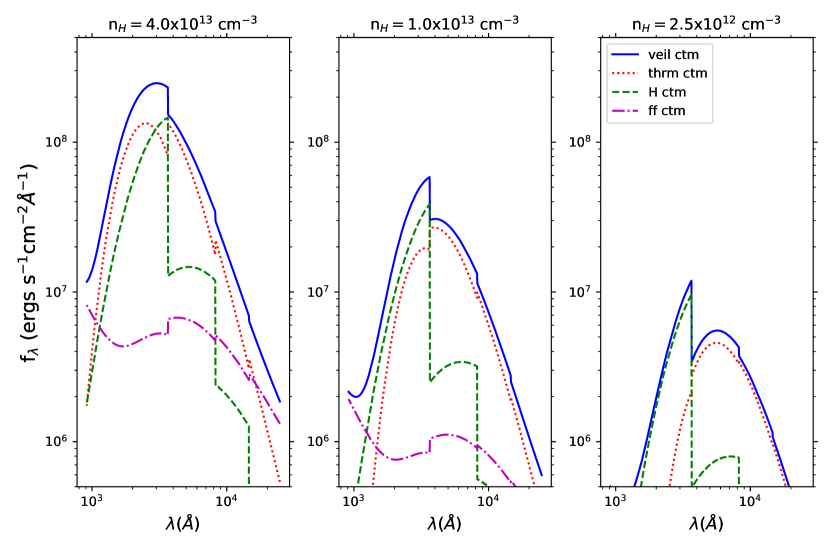
Figure 1 illustrates the emergent energy distributions obtained using case a results for the 3 values of = 300 km s-1. Besides the energy distribution of the veiling continuum (solid line), those of its constituents, namely, the thermal continuum (dotted line), the H continuum comprising the Balmer, Paschen, and Brackett continua (dashed line), and the free-free continuum (dot-dashed line) are also shown. The most conspicuous feature in the veiling continuum is the Balmer jump, which increases in magnitude as , and accordingly, decreases. The Paschen and Brackett jumps are also noticeable. All of them are, of course, much more prominent in the plot of the H continuum by itself. The thermal and free-free continua, on the other hand, show Balmer, Paschen, and Brackett drops as they are absorbed at the ionization thresholds.
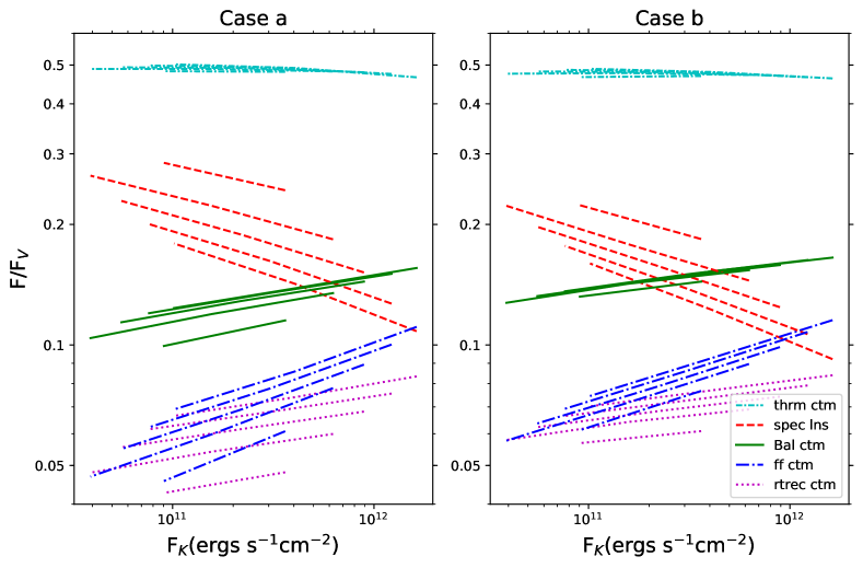
It can be gauged that the thermal continuum is the major constituent of the veiling continuum, followed by the H continuum. This is more clearly demonstrated in Figure 2, where the fractional contribution of an individual radiative component to the total emergent flux, given by with standing for , , , , or , is plotted against . Instead of the H continuum the Balmer continuum is singled out here because it is more easily extracted from observed data. The Paschen and Brackett continua will behave similarly, as and are, within 4% among the models, constant at 0.333 and 0.138 respectively. All 14 model results are exhibited, with each of the 5 lines plotted for an individual radiative component showing the variation of with at constant , whose value can be deduced from each line’s right end point.
Over the range of explored the thermal continuum accounts for close to a constant fraction of 0.5 of the emergent flux. It turns out that the hydrogen continua have opacities less than unity and most of the dominant emergent lines have opacities less than a few, so it is not surprising that roughly half of the radiative flux generated in the post-shock cooling and pre-shock photoionization zones propagate towards the star. Thus in case a the Balmer opacity has the highest value in model 1, equalling 0.266 and 0.45 in the post-shock cooling and pre-shock photoionization zone respectively, and it scales with and roughly as with 4.4, 0.8 in the post-shock cooling zone, and 2.9, 0.15 in the pre-shock photoionization zone. The presented represents the emergent value, after its attenuation through the two zones, so the thermal continuum flux produced by the stellar atmosphere is actually slightly higher.
The next significant components of are the spectral lines collectively and the Balmer continuum. The prominent emergent spectral lines originate from the post-shock cooling zone, including OVI 1034Å, CIV 1549Å, CIII 977Å, and FeII UV multiplets as a whole. Their effectiveness as coolants diminishes when the temperature exceeds K. As increases from 200 to 330 km s-1, the peak post-shock temperature rises from to K. Consequently the fractional contribution of spectral lines to the veiling flux, , falls as increases. Conversely , as well as and , rises with increasing , since the effective cooling lines at temperatures K have photon energies above 13.6 eV and they ultimately produce ionizations of H and He, leading subsequently to free-bound and free-free emission.
At a fixed also falls as increases, but the decline is gentler. Using case a to illustrate, a factor of 4.3 increase in , via increasing from 200 to 330 km s-1, produces an increase in by a factor of . On the other hand, a factor of 4 increase in via increasing produces an increase in by a factor of . This weaker dependence of on is largely because in the post-shock cooling zone OVI 1034Å, NV 1240Å, and CIV 1549Å have opacities that increase little with increasing . Over an increase in by a factor of 16, their combined flux increases almost proportionally, by a factor of . On the other hand the FeII UV multiplets and hydrogen lines are optically thick. Their combined flux increases by a factor of only . Summing all the spectral line fluxes together, increases by a factor of .
Case a and case b clearly have their biggest contrast in the degree of contribution from spectral lines. The full incorporation of dielectronic recombination in case b causes more rapid recombinations among heavy elements. The lower OVI, NV, CIV abundances as a result reduce the efficacies of OVI 1034Å, NV 1240Å, and CIV 1549Å emission as coolants and produce a smaller . The contrast between the two cases is stronger when is lower, reflecting the greater effectiveness of those line emission in cooling as the temperature falls from K.
As mentioned earlier, and are nearly constants, so the plots of and with respect to variations in and will be almost identical to those of . Together the three H continua account for 14.4 to 23.2 % of in case a and 19.2 to 24.6 % in case b within the covered parameter space. Over a factor of 41.6 in the span of their fractional contribution varies little comparatively.
The magnitudes of , , , , and depend on the strengths of their respective emission rate coefficients. Their responses to variations in and , however, are all similar, as each of them depends on density squared, and their combined flux is tied to and through the total sum being . Slight differences among the , , and plots seen in Figure 2 arise primarily from the different dependences of the respective continuum emission on temperature.
The free-free continuum flux accounts for of the total veiling flux. Its spectral energy distribution, as seen from Figure 1, is also relatively flat at optical wavelengths. It will be difficult to discern from observational data its presence as a constituent of the veiling continuum.
Fluxes from H, He, and He+ recombination continua add up to . Their respective fractional contributions are roughly 0.620.03, 0.330.04, and 0.050.02 among the 14 models in both cases a and b. The hydrogen continua contribute at longward of Å. Their presence will not be readily isolated from the stronger underlying stellar continuum.
Parts of the He+ continua have thresholds identical to the H Balmer, Paschen, and Brackett edges. Incorporating their spectral energy distributions, however, will add no more than 0.6% to the H continuum plots in Figure 1. Among the included He continua the one produced from recombinations to energy level is the strongest. It has a threshold at Å, close to the H Balmer edge, and a strength 6% of the Balmer continuum.
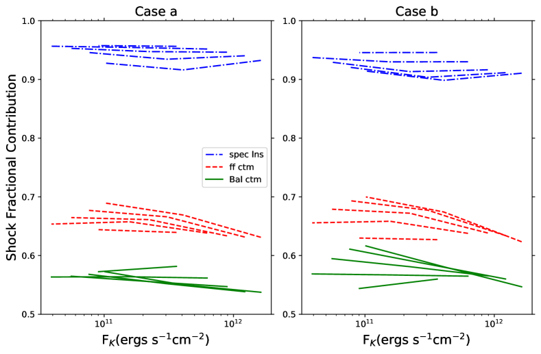
It should be noted that, whereas the emergent spectral line flux originates almost exclusively from the post-shock cooling zone, , , , , and are generated in both zones. Thus each of the noted continuum flux has two components whose strengths and dependences on and are different because the two zones have very different temperature distributions and ionization structures. Figure 3 shows the fractional share contributed by the post-shock cooling zone to , , and . Over 90% of the emergent spectral line flux originates there. This is because in the pre-shock photoionization zone the important cooling lines have high opacities, causing their photons to escape preferentially in the direction towards the star. Those with 13.6 eV, like HeII 304Å, and HeI 584Å, will cause photoionizations in the post-shock cooling zone while the rest will be absorbed by the stellar atmosphere, ultimately contributing to the emergent thermal continuum. Their combined flux is 5-8 times the flux of spectral lines emergent from the pre-shock photoionization zone.
The post-shock cooling zone is also the bigger contributor to , , , and . The ionizations of He and H there are effected first by collisions with electrons and subsequently through photoionizations. The flux of spectral line photons producing photoionizations is about the same for both zones. The temperature in the pre-shock photoionization zone, on the other hand, is K, much less effective in producing collisional ionizations. The much higher range of temperature present in the post-shock cooling zone also favors free-free emission over free-bound recombination, and produces a higher fraction of than .
3.2 Diagnostics of and
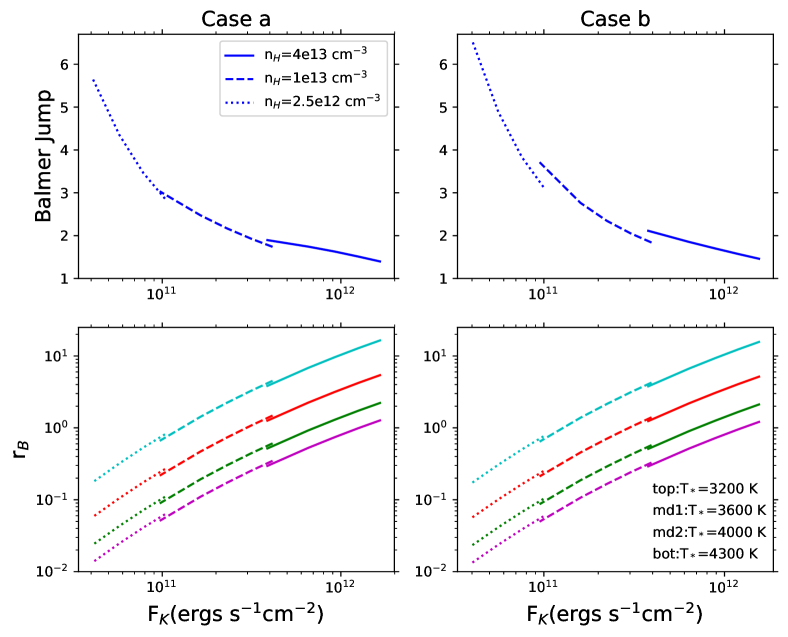
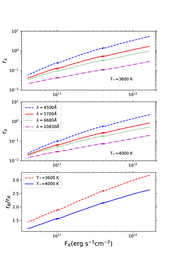
From Figure 1 it is seen that the most conspicuous feature of the veiling continuum is the Balmer jump, and that its magnitude appears to increase as , and correspondingly , decreases. The Balmer jump (BJ) is defined here as the ratio of the flux in energy bin just above the Balmer ionization threshold to that in the energy bin just below. This apparent trend is explored fully in Figure 4 which plots BJ as a function of for both cases a and b. The individual points with the same model parameter of are linked together to aid visual inspection. Because each model result is tied to its model and, as noted earlier, the discrepancy between and varies among the models, for uniformity the value of plotted is set to the value of in this and subsequent plots.
Figure 4 clearly shows that BJ depends primarily on . Thus models 5 and 6 have equal to 200 and 330 km s-1 respectively but close values of BJ(), being 1.9() and 1.74( ergs s-1 cm-2) respectively in case a. The same situation is true for models 10 and 11. This direct dependence of BJ on can actually be anticipated from Figure 2. There it is seen that both and have close to a linear dependence on while the dispersions caused by variations in are comparatively small. Hence BJ is a good diagnostic of but not or individually.
The rise of BJ as falls is readily understood from the plots of the thermal and H continua in Figure 1. The H continuum shows that at the Balmer edge the jump up from the Paschen continuum is big and slightly higher as decreases. When falls, its flux density at the Balmer edge drops roughly proportionally, as seen from Figure 1. The corresponding flux density of , on the other hand, responds much more sensitively. To illustrate, with decreasing from to cm-3 in Figure 1, falls by a factor of 16, its black-body temperature drops by a factor of 2, from to K, but its at the Balmer edge drops by a factor of 45. This strong sensitivity of the thermal continuum flux density at 3648Å to its black-body temperature over the explored parameter space is largely responsible for the higher BJ in the veiling continuum as , and correspondingly , decreases. A second contributing factor is the lower Balmer continuum opacity through the two zones, which reduces the Balmer drop in the thermal continuum, as and decrease.
Comparing the veiling and thermal continuum plots in Figure 1, it is seen that shortward of 3648Å the thermal continuum contributes only a fraction of the veiling continuum, as the Balmer continuum is a significant contributor. Longward of 3648Å , however, the thermal continuum provides the bulk of the veiling continuum. Since depends primarily on the veiling continuum flux density at a wavelength Å will also be a useful signpost of . Its utilization, however, involves knowledge of the surface area covered by the accretion shocks. Taking the latter to be , with being the area covering parameter, the ratio of the veiling continuum flux density to underlying stellar continuum flux density is . Approximating by a black-body of temperature , Figure 4 plots at =4500Å, denoted by , versus for =0.01 and = 3200, 3600, 4000, and 4300 K. It is evident that, besides BJ, is another good diagnostic of that observational data can provide.
Making use of the BJ versus and versus plots together, both and can be deduced. Once the underlying stellar continuum is extracted from the observed continuum and the veiling continuum uncovered the BJ in the veiling continuum and the observed value are obtained. The former points directly to which, in conjunction with the effective temperature of the underlying stella continuum, points to the model value for =0.01. The ratio of the observed to model times 0.01 then yields for the observed star.
Figure 4 shows the BJ - and - relations for both cases a and b. They are very similar. In deducing accretion luminosities and s for a selection of 10 stars in the next section the case a relations will be applied.
The - relation is chosen together with the BJ - relation to deduce because, as seen from Figure 1, the veiling continuum is strong at 4500Å and may be more readily separated from the underlying stellar continuum there. In principle other - relations can be used. Figure 5 shows such relations for =5700, = 0.01 and considering values of 3600 and 4000 K. The ratio of two s is independent of and is therefore a direct diagnostic of once the effective temperature of the underlying stellar continuum is determined. This is illustrated in Figure 5, using with denoting at =5700Å. There is an anti-correlation between BJ and in that a higher BJ entails a lower . This can provide a self-consistency check on the model calculations.
3.3 Selected Model Results
In Figures 2-5 model results have been connected together to aid visual inspection of relationships. They are actually discrete entities of the 14 models. Several important ones are listed here in Table 2 for ready reference.
3.4 Model Refinements
The BJ - relation indicates that BJ increases as decreases. It reaches a value of 6 at the lowest value of investigated. Observed BJs from data samples of Gullbring et al. (2000), Ingleby et al. (2014), and Manara et al. (2016), however, are less than 3. The high model BJ values at low s are likely caused in part by not taking account of the emergent flux from the stellar interior at the accretion spot. When the flux of the veiling thermal component, , is not much higher than , the stellar atmosphere will be heated comparably by emergent flux from below and incident flux from the post-shock zone above. A better approximation of the emergent thermal continuum at the accretion spot is then a single black-body component with a combined flux of () rather than two components with two black-body temperatures as tacitly assumed in the presented model calculations. To explore the consequential effects on BJ and , models 9, 12, and 14 of case a are repeated with the emergent stellar interior flux included in the calculation. Two values are considered. Cases 1 (C1) and (C) have K and cases 2 (C2) and (C) have K. C and C refer to new calculations with included while C1 and C2 refer to the original ones. The values of models 9, 12, and 14 correspond to black bodies of temperature 6167, 5146, and 4340 K respectively. When is added, with K, the resulting thermal continua have temperatures of 6423, 5562, and 4971 K. Emergent fluxes of other veiling constituents, namely , , etc, change little, by %. The thermal continuum flux density at the Balmer continuum threshold is very sensitive to its temperature, however, so BJ is the most affected. Table 3 lists the resulting BJ and also Paschen jump (PJ) in each of the different cases. It is seen, as expected, that if the C and C BJs are plotted in Figure 4 the rise of BJ with decreasing is slower, more so for K. The variation of PJ with within each individual case is itself weak, and so is its variation between cases.
Besides BJ, is another result that depends on the veiling continuum level and hence also responds sensitively to the inclusion of the emergent stellar interior flux. Assuming a of 0.01 for the accretion shocks, and in the same 4 cases are also listed in Table 3. As expected, is more strongly affected than , as the veiling continuum level at 4500Å is more sensitive to the thermal temperature than that at 5700Å.
The above discussion brings out a shortcoming of our model, the crude treatment of the response of the stellar atmosphere to the incident radiation from the accretion shock. At the end of the post-shock cooling calculation the spectrum of photons less energetic than 13.6 ev propagating towards the star is known. A stellar atmosphere subroutine that calculates the emergent stellar spectrum can be modified to include the above incident spectrum as additional input and produce accurately the resulting emergent continuum energy distribution, particularly at the Balmer ionization threshold. The two BJs obtained in Table 3 without and with included as emergent flux likely constitute upper and lower bounds, as the assumption of plane-parallel geometry and one-dimensional radiative transfer ignores the angular spread in photon emission. In all likelihood the radiation from an accretion spot propagating towards the star is incident upon an area larger than the actual size of kinematic impact, so the temperature characteristic of the resulting emergent thermal continuum will lie between the two black-body estimates obtained without and with added to .
This additional uncertainty in the determination of and can be ameliorated in future model applications. The simple procedure used earlier in Section 4 can provide initial estimates of and . Thereupon the whole veiling continuum energy distribution from a model or from interpolation between models can be combined with the adopted stellar continuum template to produce fits to the actual observed continuum spectrum to refine those estimates and maybe even the extinction measure. The model output includes the energy distribution of the thermal component, the total incident flux on the stellar atmosphere, and the total Balmer, Paschen, and Brackett opacities through the post-shock and pre-shock zones. The emergent stellar interior flux, , can then be readily included, and the new used to assess additional error margins of and inherent in our model calculations.
4 Comparison Of Model Continuum Results With Observations
In this section the model BJ - and - relations are applied to 10 T Tauri stars to determine for each of them the accretion luminosity and surface covering factor of the accretion shocks. Gullbring et al. (2000) have assembled optical spectra from Gullbring et al. (1998) and UV data from IUE Archive and procured the observed spectral energy distribution of BP Tau from 1400 to 5400Å, making this star a prime candidate for theoretical modelling. The observations of Ingleby et al. (2014) extend in wavelength from 9500Å shortwards to 3300Å, and include 1800-2600Å UV data for a couple of objects. From their sample the stars SO 1036, SO 540, and CVSO 58 are selected for the broad range covered by their BJs. Manara et al. (2016) have observed a large sample of stars and presented for each the reddening-corrected observed spectrum as well as the underlying stellar continuum template and the excess or veiling continuum energy distribution. From their sample TW Cha, T3, and VW Cha have a broad range in their BJs and the same effective stellar temperature of 4060 K, and are selected. Three other stars, ESO H562, T3-B, and T40 also have a broad range in their BJs, but their effective stellar temperatures range from 3415 to 3780 K, and they are also included. In addition to these 10 stars whose veiling continua are being modelled there are 14 stars with values determined for between 4883 and 10830 Å (Fischer, Edwards, Hillenbrand & Kwan 2011). These versus plots are also compared with the ones produced by accretion shock models.
Table 4 lists the important stellar properties of the 10 selected stars collected from the above-mentioned references. They include stellar distance , radius , and effective temperature of the underlying stellar continuum. When the item is not directly available, it is determined by making use of other information present, such as stellar spectral type and luminosity. The flux density ratio of the veiling continuum to underlying stellar continuum at 4500Å is also estimated from visual measurements off the pertinent plots published, and listed.
The presence of an accretion disk implies that the observed stellar solid angle will depend on viewing angle and the size of the disk truncation gap. Letting be given by , the viewing factor can be estimated by comparing the observed flux density of the adopted underlying stellar continuum with that expected from an unobscured one. Making the comparion at 6000Å where approximation of the unobscured stellar continuum by a black-body of temperature is suitable, this viewing factor is calculated for BP Tau, SO 1036, SO 540, and CVSO 58. For the six objects selected from Manara et al. (2016) the comparison is made at 4600Å because the plotted spectra do not extend beyond 4630Å. This estimate is denoted by to indicate its approximation of the correct obtained with the adopted stellar continuum template. Its value for each star is listed in Table 4.
The viewing factor is necessary to convert the model result to an accretion luminosity for comparison with the observed value. The latter has been determined by Manara et al. (2016) for each of their observed stars via use of a multi-grid fitting procedure in conjunction with a slab model of the hydrogen continuum emission to estimate, in addition to requisites like visual extinction and appropriate underlying stellar template, the total veiling flux from that observed between 3300 and 7150Å and thence the observed accretion luminosity. The latter is denoted by , and its value obtained by Manara et al. (2016) is listed for each of their six stars selected.
The observed BJ in the veiling continuum of a star points to and from the relation the area covering factor can be found. The observed accretion luminosity from the theoretical model to be compared with the listed value is then given by . If the stellar surface obscured by the accretion disk is similarly covered by accretion shocks, the accretion luminosity for the entire star is then given by . Gullbring et al. (2000) and Ingleby et al. (2014) report such values using the theoretical models of Calvet & Gullbring (1998) and those values for the four stars selected are listed.
Approximation of the underlying stellar continuum by a black-body continuum means that the values of and produced by our modelling of the observed veiling continuum are actually given by and respectively. If, at the wavelength chosen to determine the viewing factor and at 4500Å , the black-body flux density is and times respectively that of the adopted stellar template, then the correct viewing factor is , and the correct area covering factor is . Our model values of and will need to be multiplied by and respectively.
The correlation of BJ with is tight, particularly for between 240 and 330 km s-1. An observed BJ will point directly to a via interpolation between the model results. This procedure is not followed here in view of the approximate estimates of , BJ, and from published plots. Instead the model with its BJ closest to the observed value is chosen to simulate the observed veiling continuum. The corresponding model number, BJ, and being set equal to , as well as the derived values of , , and , are listed for each selected star in Table 4.
4.1 BP Tau
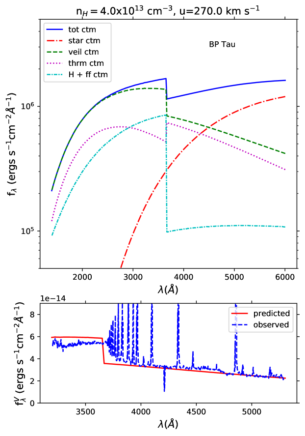
Gullbring et al. (2000) show in their Figure 1 the underlying stellar continuum employed, the veiling continuum from the theoretical modelling of Calvet & Gullbring (1998), and their sum to compare with the de-reddened observed spectral energy distribution from 1400 to 5400Å. Also shown are their two constituents of the veiling continuum, which are the emission from the heated photosphere below the shock and emission from the pre-shock and attenuated post-shock regions. Following their lead, Figure 6 plots a black-body spectrum of temperature 4000 K, the veiling continuum produced in model 3 multiplied by a factor , and their sum. To compare directly with the corresponding plots in Figure 1 of Gullbring et al. (2000), the vertical scale of Figure 6 needs to be multiplied by the factor . Thus at 6000Å the black-body flux density, the veiling continuum flux density, and their sum will have observed values of , , and ergs s-1 cm-2 Å-1 respectively. Also plotted in Figure 6 are the two constituents of the veiling continuum, namely the thermal continuum, and the sum of the H continuum and free-free continuum.
Comparing the black-body spectrum with the underlying stellar continuum template indicates that their difference begins to occur at 4000Å and increases towards shorter wavelengths. At 6000 and 4500Å the corresponding values and are reasonable estimates of and then. In overall shape from 1400 to 6000Å the total continuum spectrum shown in Figure 6 appears to reproduce that actually observed fairly well. Gullbring et al. (1998) have presented the extracted excess spectrum of BP Tau in finer detail from 3200 to 5300Å in their Figure 7. To compare with it, the bottom part of Figure 6 plots on the same scale the model veiling continuum distribution after multiplication by the factor to bring it into the observed realm. Longwards of 3700Å , it reproduces the observed excess continuum distribution well, but shortwards of the BJ, the model veiling flux density is about 10% higher.
Examining the model results in greater detail through the veiling continuum constituents, it is seen that the BJ in the model H continuum is considerably higher than that present in the H continuum of Gullbring et al. (2000) that comprises pre-shock and attenuated post-shock emission. At the same time emission from the heated atmosphere has a Balmer drop in our model but a BJ in theirs. These differences most likely arise from the different demarcations of the post-shock cooling zone from the heated atmosphere. In our model the post-shock cooling zone ends when the hydrogen ionization fraction drops below 0.2%. In the case of BP Tau when this occurs the temperature is K, the hydrogen Lyman continuum opacity and nucleon column density as measured from the shock front are and cm-2 respectively. This demarcation ensures that all the ionizing photons propagating towards the star are absorbed and their heating effect and the ensuing hydrogen recombination properly taken account of within our numerical calculation procedure. If Calvet & Gullbring (1998) end their post-shock region earlier, a fraction of the ionizing photons will photoionize hydrogen in their heated atmosphere zone and the emission from there will contain Balmer continuum photons and exhibit a BJ.
As gauged from Figure 6 the model veiling continuum appears to match the observed excess continuum about as well as that presented by Gullbring et al. (2000). The derived values of and , however, are quite different. They are ergs s-1 cm-2 and 0.444 from our model versus ergs s-1 cm-2 and 0.138 from theirs. The area covering factor is similar though, being and respectively.
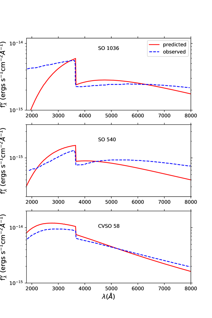
4.2 SO 1036, SO 540, CVSO 58
Ingleby et.al. (2014) have presented in their Figure 4 the de-reddened observed CTTS spectrum and adopted WTTS template for each of their eight observed stars, and in their Figure 5 the corresponding extracted excess continuum. From these two figures the quantities and are estimated for each of the three selected stars. Then to simulate the excess continuum, a theoretical model is chosen based on the magnitude of its BJ. The model number, BJ, = value, and the derived , together with and , are listed in Table 4. Two stars have stellar templates with an effective temperature of 4000 K while the third, SO 1036, has 3700 K, so the and values may not be far off. Figure 7 plots for each star the predicted excess continuum distribution that will be observed according to the parameters , , and on the same scale as that used for the corresponding observed spectrum. Also plotted is the excess continuum obtained by Ingleby et al. (2014), upon application of the Calvet & Gullbring (1998) accretion shock models, that provides the best fit to the observed data. For SO 540 the actual observed excess continuum extends in wavelength from 8000 to 1800 Å, but for SO 1036 or CVSO 58 it only extends to 3300 Å. Overall, the comparison between model and observed spectra is fair.
Model 9 is used to simulate the excess continuum of SO 1036. The value of this model is low and taking account of the emergent stellar interior flux is relevant. The results illustrated in Table 3 indicates that for = 3600 K, which is close to SO 1036’s, the new BJ is smaller than the original one by 9.4 and the new is higher than the original one by 13.6, so the corresponding will be smaller by the same percentage than the original one listed in Table 4.
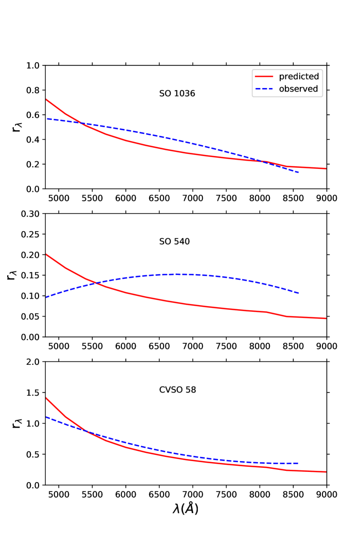
Ingleby et al. (2014) have also plotted in their Figure 3 the veiling as a function of wavelength for each of their observed stars, employing two different WTTS as templates for unveiled absorption lines. To compare with the data points of the three selected stars, Figure 8 plots on the same wavelength scale the obtained in the model using a black-body spectrum to approximate the underlying stellar template, and the fit to the data points derived by Ingleby et al. (2014). Given the large scatter of the data points, being more than about the fit, the predicted dependence is in reasonable agreement with that observed.
The stars SO 1036, SO 540, and CVSO 58 are selected for the decreasing order in BJ magnitude seen in their respective veiling continuum. According to the BJ - relation the derived is consequently in ascending order. The area covering factor is arbitrary, so there is no trend in the derived and thence . Comparing these model results, listed in Table 4, with the corresponding values of Ingleby et al. (2014) is somewhat hampered by their use of two components, one of high and the other of 10-100 times lower. For SO 1036 our (ergs s-1 cm-2) of 1.64 1011 is roughly the geometric mean of their two components of 1012 and . Our () of 0.53 is quite a bit higher than their 0.1 value because our single component has an area covering factor of 2.44 10-2, about half of that occupied by their = 1010 component but much higher than the factor of 2 10-4 for their = 1012 component. For SO 540 our of 3.14 1011 is close to their high component of 3 1011, but has an area covering factor of 5.67 10-3 that is 11 times higher. Our of 0.112 happens to be close to their 0.1 value because their low component of 3 1010 has an area covering factor of 4 10-2 and contributes over 85% of their . For CVSO 58 the comparison between the theoretical models is the closest. Their high component of 1012, with an area covering factor of 5 10-3, provides the bulk of a of 0.3, while our model has a of 1.66 1012, an area covering factor of 8.56 10-3, and a of 0.5.
4.3 Chamaeleon I Stars
Manara et al. (2016) have observed and analyzed 34 Chamaeleon I young stellar objects and presented in their Figure C.1 the photospheric template, the veiling continuum from their slab model, and their sum to compare with the reddening-corrected observed spectrum for 32 of them. From this group of 32 stars six are selected for modelling. Among the remaining stars nine have 3270 K and derivations of and using a black-body spectrum to approximate the actual photospheric template will be quite inaccurate shortwards of 4600Å. Another ten have either very weak veiling continua or very small BJs to model reliably. For the six selected stars their pertinent data parameters and model results are listed in Table 4.
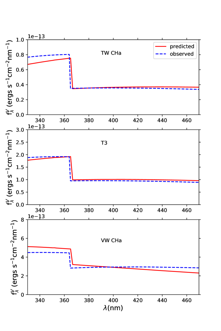
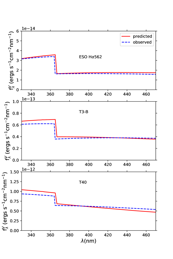
Simulation of the veiling continuum of each selected star follows the same procedure as described earlier for BP Tau and the three Orion stars. Figure 9 presents for each of TW Cha, T3, and VW Cha the predicted veiling continuum observed in accordance with the values of , , and . Following the convention of Manara et al. (2016), it is in units of ergs s-1 cm-2 nm-1 and plotted over the same wavelength range from 330 to 470 nm. These three stars all have a photospheric template with effective temperature of 4060 K, and are arranged from top to bottom in order of decreasing BJ. In the same way Figure 10 presents the model veiling continua of ESO H562, T3-B, and T40. Their photospheric effective temperatures are different, being 3705, 3415, and 3780 K respectively.
A look at Figures 9 and 10 indicates that the overall shape of the veiling continuum correlates with the BJ magnitude. Thus, at 364.8 nm the slope of the veiling continuum towards shorter wavelengths change from rising to falling as BJ increases, while at 364.8 nm the slope towards longer wavelengths change from falling to rising, though less noticeably. This correlation is actually more conspicuous in Figure 7 where the plotted wavelength range, from 1800 to 8000Å , for the three Orion stars is more extensive. It is also evident from the veiling continua illustrated in Figure 1 for the three models with = 300 km s-1 and different values. The comparison of model results with a large number of observational data brings this correlation more into focus. It also sets up a strict test of the theoretical model.
Overall the theoretical veiling continua of the six selected stars compare reasonably well with the corresponding observed excess continua shown in Figure C.1 of Manara et al. (2016) that are generated by their slab model through a multi-grid fitting procedure involving also the visual extinction and photospheric template. From Table 4 it is seen that the derived viewing factors cluster between 0.6 and 0.7 except for T3-B which has = 0.42 and also the lowest of 3415 K among them. Most likely the black-body spectrum overstimates the photospheric template at 460 nm, and the derived will be an underestimate. For the same reason the derived will be an overestimate. Interestingly, because is given by its derived value will be less affected, as and are evaluated at fairly close wavelengths. The derived , on the other hand, will be affected just as .
Comparing the model with the corresponding value of Manara et al. (2016) the former is higher in each case, by a factor ranging from 1.26 for VW Cha to 1.79 for ESO H562. One obvious cause for this result is the inclusion of spectral line fluxes in the total veiling flux in our model. An additional cause may come from He and He+ recombination and free-free continua being part of our veiling continuum, but they may not be a part of the continuum generated by the slab model of Manara et al. (2016). The two causes together can lead to our being higher by a factor of 1.3. Taking this factor into consideration, the closeness between the observed and model values is fairly remarkable.
Among the remaining stars in the sample of Manara et al. (2016) several, like CT Cha A, have BJs smaller than the smallest BJ obtained in the 14 models. An additional model with = 300 km-1 and = 1014 cm-3 is run, and it has a BJ of 1.21 and of 3.11 ergs s-1 cm-2, so the BJ - FK relation will extend.
In producing model veiling continua to compare with observed data, case a results have been used. If, for each of the ten selected stars, the same model is used but with case b results the derived is 3-5% higher than, while is within 1% of the corresponding case a values.
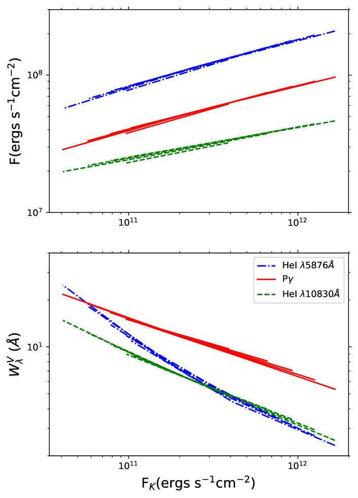
4.4 versus Plots of 14 Stars
Fischer, Edwards, Hillenbrand & Kwan (2011) have presented in their Figure 1 versus plots of 14 stars in their effort to determine the excess continuum emission from 0.48 to 2.4 of their sample of 16 classical T Tauri stars. The value of depends on the underlying stellar continuum energy distribution which is approximated by a black-body spectrum in our model, and two values, 3600 and 4000 K, are chosen to illustrate. It also depends on the surface covering factor of the accretion shocks and, to eliminate this dependence, the ratio , with being evaluated at is plotted as a function of from 0.48 to 1.08 in Figure 11. The comparison between model and observed plots then rests on the shape or slope of each curve. Results from models 1, 6, 9, and 14 are presented to demonstrate the dependence on . In particular, for 4000 K, at 0.48 spans from in model 1 to in model 14.
Looking at the observed plots it is seen that the polynomial fits of 7 stars (BP Tau, CY Tau, DF Tau, DK Tau, DL Tau, DO Tau, LkCa 8), if replotted with normalized to 1, will be similar to the model curves. Two stars (DR Tau, HN Tau) have values of , excepting , that can also be reproduced by models. The plots of two stars (AA Tau, BM And) are flat from 0.48 to 8.7 . Allowing for uncertainties in the observed values, they can be considered as being close to the curve of model 14 whose is the lowest considered. The star DG Tau has its plot from 0.48 to 0.8 like a model curve, but also an upturn in from 0.8 to 0.87 that contradicts. The remaining two stars (AS 353A, CW Tau) do not have clearly defined plots to make a valid comparison, as neighboring values differ widely.
Overall the accretion shock model can account for a large fraction of the observed plots. For full affirmation of the model the BJs in the veiling continua are needed to verify if the s implied separately by the plot and the BJ value are the same. For those objects whose values challenge the model their veiling continua need to be determined from UV to infrared wavelengths in order to compare fully with those generated by accretion shocks.
5 Line Fluxes And Shock Parameters
The accretion shock calculation produces line fluxes in addition to continuum energy distributions. Line emission originating from the post-shock cooling zone have smaller widths in comparison with that originating from the pre-shock photoionization zone which suffer a greater Doppler broadening. They appear as NCs of observed profiles. Among the prominent emergent lines in our model their NC fluxes are also stronger than their broad component (BC) fluxes produced in the pre-shock zone as they are generated at a higher temperature and their optical depths in the post-shock zone are much smaller. The NC fluxes of prominent UV lines, like OVI 1034Å and CIV 1549Å are stronger than those of optical lines, but their observed values depend sensitively on the extinction measure. Optical NC fluxes, on the other hand, are independent of the extinction measure when expressed in equivalent widths relative to the continuum flux densities. The HeI 5876Å NC, in particular, is a prominent line in the model calculation, and among its observed profiles most have either dominant NCs or ones that are easily isolated from BCs (BEK01). It is therefore a prime candidate for verification of the model calculation through comparison with observed data.
Figure 12 shows the dependence on of the 5876Å NC flux (top panel) and its equivalent width relative to the veiling continuum flux density (bottom panel). The NCs of 10830Å and P are also presented because the 10830Å line, with its lower level being the metastable state, bears key information on the physical conditions leading to population of the He excited levels, and P is always observed along 10830Å . Thus the 5876Å/10830Å and P/10830Å flux ratios provide additional checks on the accretion shock model.
All three line fluxes are insensitive to either or alone, and increase only slowly with increasing . An increase in of 40 produces an increase in the HeI 5876Å NC flux of 3.6. This is because the He and H optical emission occur mostly after the shocked gas has cooled to 2.5 K and are close to being thermalized owing to the high electron densities. For a given model flux, the observed flux depends on . The equivalent width relative to the veiling continuum flux density, on the other hand, does not. Either result can be used for comparison with observed data.
BEK01 presented in their Figure 4 31 observed NC data in a log[x(1 + )] versus log plot, where here denotes the NC equivalent width in Å with respect to the total (photospheric + veiling) continuum, and at = 5700 Å. If denotes the photospheric flux density (ergs s-1 cm-2 Å-1) at wavelength , then the NC flux is given by x(1 + ), and the veiling continuum flux density by at = 5876 Å. Taking as an approximation of , the plot then shows the relation between the NC flux and the veiling continuum flux density.
The model results can be presented in a similar way and Figure 13 is a reproduction of the top panel of Figure 4 in BEK01, together with model tracks derived from the model calculations. The latter are obtained with = 0.01, increasing from 4.11x (model 14) to 1.66x10¹² ergs s-1 cm-2 (model 1) in case a, and for three values of 3600, 4000, and 4300 K. The solid line marked , depicting the trajectory for an equal increment in each co-ordinate, illustrates how each model track will shift for s different from 0.01, as both x(1 + ) and are proportional to . The area swept by the model tracks as they slide along the direction of varying then outlines the model domain wherein observed data points can be reproduced by one of the 14 models. Alternatively a data point can slide along its own line of variation until it intercepts the model track appropriate to its to determine the of the shock model that will reproduce it. The ratio of its to the at the intersection point times 0.01 then yields .
The 31 observed stars are sorted into four groups according to the ratio of BC to NC equivalent width (BC/NC). Group 1 has 9 objects, marked +, with each having a prominent NC and no or only a very weak BC (BC/NC 0.1). Their profiles are shown in Figure 1b of BEK01. Group 4 with 6 objects is characterized by a NC that is absent or much weaker than the BC (BC/NC 8). Marked , they are, from top to bottom, DR Tau, DL Tau, AS 353A, DG Tau, CW Tau, and HN Tau. Each of the remaining objects has easily identifiable NC and BC. They are subdivided into two groups, group 2 with 10 objects having BC/NC between 0.4 and 1.4, and group 3 with 6 objects having BC/NC between 2.5 and 7.2.
Several observations are noted from the spatial distribution of the data points relative to the model tracks: 1) the objects in group 1 all lie within the model domain; 2) 5 of the 6 objects in group 4 are far to the right of the domain as measured by their perpendicular distances from the solid line of varying ; 3) comparing the four groups, the perpendicular distance of each group from the solid line increases as BC/NC increases.
Two inferences follow from the above findings. First, the group 1 objects or other observed stars with dominant 5876Å NCs can provide a test of the model calculation by verifying if the pair of (, ) values indicated by the NC matches that deduced from modelling the excess continuum. Second, assuming validity of the model calculation, the 14 models clearly fail to replicate some of the data points, particularly those in group 4. One possible explanation is that those points, when extended along their lines of varying , just indicate that accretion shocks with s much higher than 1.66x10¹² ergs s-1 cm-2 and s less than 0.01 are needed. This suggestion can be verified readily by examining the BJ and shape of the excess continuum from 3648Å to 1 , as both of them correlate strongly with (cf. Figs. 4 & 11). Another possible explanation is that accretion shocks contribute only a small fraction of the excess continuum in those objects. This fraction can be estimated by extending the data point horizontally to the left, thereby ensuring a constant NC flux, until it intersects the lines of varying extending from the 14 model points that generate the plotted track of the appropriate . The intersection points provide 14 possible pairs of (, ) that can reproduce the observed NC flux. The ratio of the at each intersection point to the data point then gives the fractional contribution from accretion shocks to the observed excess continuum at 5700Å in each case.
The second explanation is preferred here, based on additional information conveyed by the BC profiles, particularly those in groups 4 and 3. Their blue-shifted emission, with blue-shifted centroids and strong blue wings, indicate an origin in outflowing gas (BEK01), and observed 10830Å profiles, with broad blue absorptions, provide direct confirmation (EFHK06). Then local excitation calculations find that while temperatures of K are sufficient to produce the observed 5876Å emission, UV photons that ionize HeI are needed to populate the metastable state via recombination and cascade (Kwan & Fischer 2011), and such is the case for the NC emission. The absence of or much weaker broad emission observed among group 1 objects indicates that UV photons generated from accretion shocks produce comparatively little emission in either the pre-shock photoionization zone, a result confirmed by our model calculation, or the full magnetospheric accretion columns. Thus the UV photons producing He ionization in the outflow have a different origin. These photons will also cause emission of hydrogen Balmer, Paschen, and other recombination continua and possibly a thermal-like continuum if part of the continuum and line radiation thus produced propagate towards the star and their absorbed fluxes re-emerge as radiation at lower energies. This second origin of UV photons and excess continuum is likely associated with the energy source propelling the outflow.
6 Discussion
The main findings of this paper on continuum emission are the BJ - and relations. By means of them the values of and the surface covering factor can be deduced. Other results are the percentages of the total veiling flux contributed by the Balmer continuum, spectral lines, and other constituents. The relative importance between the post-shock cooling zone and the pre-shock photoionization zone in generating the various veiling components, particularly the spectral lines, is also an outcome.
Comparisons between model and observed veiling continua for 10 T Tauri stars show that our accretion model can reproduce those observed data fairly well. Our derived values of and for BP Tau and the three Orion stars differ considerably from those obtained through application of the shock model of Calvet & Gullbring (1998). This arises largely from the difference in the dependence of BJ on between the two models and the use of multiple shock components by Ingleby et al. (2014). For the 6 stars in Chamaeleon I our s are about 27-78% higher than the corresponding values obtained by Manara et al. (2016).
The use of multiple components to fit the excess continuum is now well established (e.g., Pittman et al. [2022]). This procedure is not without issues. First each component has two parameters, a that governs the shape of the continuum and a that provides the overall magnitude. Each additional component introduces two more free parameters and the higher degrees of freedom in the fitting procedure, while producing a better fit to the data, also reduces the confidence in the derived results. Second, the accuracy of the continuum energy distribution for each calculated by Calvet & Gullbring (1998) has not been established, so its inaccuracy can by itself cause the poor fit with a single component, further diminishing the merit in the goodness of fit with multiple components. In the end, the derived (, ) values from single or multiple component fitting of the excess continuum need to be confirmed, and spectral line fluxes provide a means. A particular shock model calculation will gain credence only when the set or sets of (, ) obtained from fitting an excess continuum can also reproduce the observed flux of a prominent line formed in accretion shocks.
The alternative shock model calculation presented here is subject to the same test criterion. As noted in 5 and seen from Figure 13, objects with dominant HeI 5876 Å NCs are prime candidates for such a test. The availability of simultaneous continuum and spectral line data through the Penellope and Ullyses programs (Manara et al. 2021, Pittman et al. 2022) makes this test feasible. Model and spectral line fluxes for each of the 14 models will be publically available and they can be used to check if the same (, ) set reproduces both the excess continuum and the 5876 Å NC flux in objects with dominant NCs. The HeI 5876 Å/HeI 10830 Å and /HeI 10830 Å flux ratios provide additional tests.
Figure 13 also shows there are objects, particularly those with BCs much stronger than NCs, whose NC flux, given the observed strength of their excess continuum, cannot be reproduced by the 14 models. They need either accretion shocks with s much higher than heretofore calculated or presence of a second source of excess continuum. The first proposition can be tested by verifying if the observed excess continua of those objects have BJs and s expected of accretion shocks with very high s.
While a second origin of excess continuum needs to be confirmed, the presence of another source of UV photons besides accretion shocks is clearly indicated on the following grounds. The UV photons produced in the post-shock zone facilitate the optical He emission there by populating the metastable and levels through recombination and cascade that ensue after photoionizations. Collisional excitations from the metastable levels then lead to strong NC emission. Those UV photons that propagate away from the star apparently cause little He emission in either the pre-shock zone or the full magnetospheric accretion columns, as evinced by the 9 objects with dominant NCs and little BCs (BEK01). Among the remaining 22 objects in the data sample, which all have obvious BCs, 11 of them occupy in Figure 13 positions indicating that their NC strengths can be accounted for by the 14 model calculations, just like the 9 objects mentioned earlier. Some of the BCs are stronger than their corresponding NCs. If the accretion shock is the only source of UV photons, it is difficult to fathom how the same realm in (, ) parameter space for the 20 objects generate such drastically different effects at regions farther away. Examination of the 11 BC profiles indicates that several of them have characteristics, like blue-shifted centroids and strong blue wings, that signal line emission from outflowing gas. This kinematic flow is located beyond the accretion columns of infalling gas and UV photons from accretion shocks will have a greater difficulty affecting it because of intervening attenuation and a greater spatial dilution. This predicament faced by accretions shocks as the sole source of UV ionizing photons is even more severe for the remaining 11 objects in the sample, which have BCs more than 2.5 times stronger than NCs and broad blue-shifted profiles indicative of outflow. In contrast, inferring presence of a second origin of UV ionizing photons whose strength correlates with the flux of the broad He emission makes better sense, and this second origin is likely associated with the energy source propelling the outflow that emits the broad blue-shifted He emission.
The second UV radiation source appears to influence hydrogen line emission also, as the observed P profiles show outflow characteristics when HeI 10830Å profiles do (cf. Figs. 3 & 4 of EFHK06). Their fluxes among group 4 objects are also the strongest, with the caveat that the sample is observed much later than the HeI 5876Å sample. Hydrogen Balmer, Paschen, and other recombination continuum emission will be concurrent too. The ratio of P flux to Balmer continuum flux will likely be different from that generated in the post-shock zone, as the environment around the second UV source is very different. For one thing the UV photons have to affect a larger region, as the HeI 5876Å BC profile indicates that the outflow occupies a fairly large solid angle about the star in order that projections of radial velocities along the line of sight cover a wide span from positive to negative values. Absorption of the ionizing photons also take place at some distance from the star, and the gas densities are likely to be considerably smaller than those at accretion shocks. At the same time line and continuum emission that ensue occur over a bigger region. Those photons propagating towards the stars will be absorbed over a good fraction of the stellar surface. The re-emergent energy flux will likely have an equivalent black-body temperature smaller than that produced in the case of accretion shocks with the same total line and continuum flux incident upon the star. These conjectures can all be verified upon examination of the excess continua observed in stars with HeI 5876Å BCs much stronger than NCs.
The model results reveal that the veiling continuum energy distribution is insensitive to or individually. A higher implies a higher temperature range in the post-shock zone. Most of the spectral lines responsible for cooling of the gas at high temperatures deposit their energies at temperatures K through photoionization of H and He. The consequent H and He continuum emission from subsequent radiative recombinations then depend much on the total flux in those lines but little on their origins. Free-free emission is produced over the entire temperature range and, as seen from Figure 1, a greater fraction of its flux lies at Å than either the H or thermal continuum. This fraction depends on , but is difficult to be extracted as free-free emission constitutes a significant portion of the veiling continuum only at Å . Unlike continuum emission, line emission in the post-shock zone occur over a broad range of density and temperature, owing to the variety of ionic stages and line excitation parameters. Spectral lines whose fluxes depend differently on and can be identified. Their individual fluxes or their flux ratios will shed light on besides . This finding and other results deduced through comparisons of model line fluxes with observed spectral line data are the subject matter of a follow-up paper.
7 Acknowledgments
8 Data Availability
The important results of this paper have been presented in Figures and Tables. Extensive results, like the wavelength dependence of the excess continuum of each calculated model, are available upon request. An organized set of all the relevant data will also be available at a website accessed via https://www.stsci.edu/wfischer.
References
- (1) Adams T. F., 1972, ApJ, 174,439
- (2)
- (3) Aldrovandi S. M. V., Pquignot D., 1973, A&A, 25, 137
- (4)
- (5) Alencar S. H. P., Basri G., 2000, AJ, 119,1881
- (6)
- (7) Allen C. W., 1973, Astrophysical Quantities, Athlone, London
- (8)
- (9) Anderson H., Ballance C. P., Badnell N. R., Summers H. P., 2002, J. Phys. B, 35, 1613
- (10)
- (11) Ardila D. R., Herczeg G. J., Gregory S. G., et al., 2013, ApJS, 207,1
- (12)
- (13) Arnaud M., Rothenflug R., 1985, A&AS, 60, 425
- (14)
- (15) Avery L. H., House L. L., 1968, ApJ, 152, 493
- (16)
- (17) Basri G., Batalha C., 1990, ApJ, 363, 654
- (18)
- (19) Benjamin R. A., Skillman E. D., Smits D. P., 1999, ApJ, 514,307
- (20)
- (21) Beristain G., Edwards S., Kwan J., 2001, ApJ, 551,1037 (BEK01)
- (22)
- (23) Calvet N., Gullbring E., 1998, ApJ, 509, 802
- (24)
- (25) Davidson K., 1975, ApJ, 195, 285
- (26)
- (27) Dodin A., 2018, MNRAS, 475, 4367
- (28)
- (29) Edwards S., Fischer W., Hillenbrand L., Kwan J., 2006, ApJ, 646, 319 (EFHK06)
- (30)
- (31) Fischer W., Edwards S., Hillenbrand L., Kwan J., 2011, ApJ, 730, 73
- (32)
- (33) Gullbring E., Calvet N., Muzerolle J., Hartmann L., 2000, ApJ, 544, 927
- (34)
- (35) Gullbring E., Hartmann L., Briceo C., Calvet N., 1998, ApJ, 492,323
- (36)
- (37) Hartmann L., Herczeg G. J., Calvet N., 2016, ARA&A, 54, 135
- (38)
- (39) Ingleby L., Calvet N., Herczeg G. J., et al., 2013, ApJ, 767, 112
- (40)
- (41) Ingleby L., Calvet N., Hernndez J., et al., 2014, ApJ, 790, 47
- (42)
- (43) Johns-Krull C. M., Chen W., Valenti, J. A., et al., 2013, ApJ, 765, 11
- (44)
- (45) Johnson L. C., 1972, ApJ, 174, 227
- (46)
- (47) Kwan J., Fischer W., 2011, MNRAS, 411,2383
- (48)
- (49) Kwan J., Krolik J. H., 1981, ApJ, 250, 478
- (50)
- (51) Lodders K., 2020, Solar Elemental Abundances, in Oxford Research Encyclopedia of Planetary Science
- (52)
- (53) Manara C. F., Fedele D., Herczeg G. J., Teixeira P. S., 2016, A&A, 585, A136
- (54)
- (55) Manara C. F., Frasca A., Venuti L., et al., 2021, A&A, 650, A196
- (56)
- (57) Marr G. V., West J. B., 1976, Atomic Data and Nuclear Data Tables, 18, 497
- (58)
- (59) Montague R. G., Harrison M. F. A., Smith A. C. H., 1984, J Phys. B., 17, 3295
- (60)
- (61) Pittman C. V., Espaillat C. C., Robinson C. E., et al., 2022, AJ, 164, 201
- (62)
- (63) Raymond J. C., Smith B. S., 1977, ApJS, 35, 419
- (64)
- (65) Reilman R. F., Manson S. T., 1979, ApJS, 40, 815
- (66)
- (67) Robinson C. E., Espaillat C. C., 2019, ApJ, 874, 129
- (68)
- (69) Romanik C. J., 1988, ApJ, 330, 1022
- (70)
- (71) Sawey P. M. J., Berrington K. A., 1993, At. Data Nucl. Data Tables, 55, 81
- (72)
- (73) Seaton M. J., 1958, Rev. Mod. Phys., 30, 979
- (74)
- (75) Seaton M. J., 1959, MNRAS, 119, 81
- (76)
- (77) Shull J. M., Van Steenberg M., 1982, ApJS, 48, 95
- (78)
- (79) Sutherland R. S., 1998, MNRAS, 300, 321
- (80)
- (81) Taylor I. R., Kingston A. E., Bell K. L., 1979, J. Phys. B, 12, 3093
- (82)
- (83) Verner D. A., Ferland G. J., 1996, ApJS, 103,467
- (84)
- (85) Young P. R., Zanna G. D., Landi E., Dere K. P., Mason H. E., Landini M., 2003, ApJS, 144, 135
- (86)
Appendix A Atomic Parameters
The rate coefficients for collisional transitions between HI energy levels are those in Kwan & Fischer (2011). There it is detailed how they are obtained from Anderson et al. (2002) and Johnson (1972). The rate coefficient for collisional ionization from the ground state is obtained from Arnaud & Rothenflug (1985). Those for collisional ionizations from excited states are calculated from the formulae given in Johnson (1972). Photoionization cross-sections for the first four levels are gathered from Allen (1973) and radiative recombination coefficients from Seaton (1959).
The HeI atomic parameters used are also those in Kwan & Fischer (2011). There it is explained how the collision strengths between levels are collected from the Chianti data base (Young et al. 2003) and Sawey & Berrington (1993), the collisional ionization rate coefficients from Montague, Harrision & Smith (1984), Taylor, Kingston & Bell (1979), and Benjamin, Skillman & Smits (1999), and the radiative recombination coefficients from Benjamin et al. (1999).
For heavy elements their atomic parameters, including level excitation energies, spontaneous emission rates, and rate coefficients for collisional transitions between levels are gathered from Chianti (Young et al. 2003). Their collisional ionization rate coefficients are obtained from Arnaud & Rothenflug (1985). For hydrogenic ions their radiative recombination rates are calculated from the formula given by Seaton (1959). For the remaining heavy ions their radiative recombination rates are gathered from Arnaud & Rothenflug (1985), Aldrovandi & Pquignot (1973), Shull & Van Steenberg (1982), and Verner & Ferland (1996). Dielectronic recombination coefficients are obtained from Romanik (1988) when available, and from Shull & Van Steenberg (1982) for the others.
Photoionization cross-sections of He and heavy elements used are those in Kwan & Krolik (1981). There details are given on the use of Seaton (1958) two-term interpolation formula to fit cross-sections as a function of energy, and data collection from Marr & West (1976), and Reilman & Manson (1979).
| Model | (cm-3) | (km s-1) | (ergs s-1 cm-2) |
|---|---|---|---|
| 1 | 4 1013 | 330 | 1.63 1012 |
| 2 | 4 1013 | 300 | 1.22 1012 |
| 3 | 4 1013 | 270 | 8.91 1011 |
| 4 | 4 1013 | 240 | 6.26 1011 |
| 5 | 4 1013 | 200 | 3.62 1011 |
| 6 | 1 1013 | 330 | 4.07 1011 |
| 7 | 1 1013 | 300 | 3.06 1011 |
| 8 | 1 1013 | 270 | 2.23 1011 |
| 9 | 1 1013 | 240 | 1.56 1011 |
| 10 | 1 1013 | 200 | 9.05 1010 |
| 11 | 2.5 1012 | 330 | 1.02 1011 |
| 12 | 2.5 1012 | 300 | 7.64 1010 |
| 13 | 2.5 1012 | 270 | 5.57 1010 |
| 14 | 2.5 1012 | 240 | 3.91 1010 |
| Case a | Case b | |||||||||
| Model | BJ | BJ | ||||||||
| (ergs s-1 cm-2) | (ergs s-1 cm-2) | |||||||||
| 1 | 1.66 | 0.466 | 0.156 | 0.108 | 1.384 | 1.557 | 0.46 | 0.167 | 0.092 | 1.456 |
| 2 | 1.26 | 0.475 | 0.151 | 0.127 | 1.512 | 1.194 | 0.466 | 0.163 | 0.106 | 1.569 |
| 3 | 9.269 | 0.48 | 0.144 | 0.152 | 1.627 | 8.904 | 0.471 | 0.158 | 0.124 | 1.698 |
| 4 | 6.596 | 0.482 | 0.135 | 0.183 | 1.741 | 6.405 | 0.472 | 0.154 | 0.145 | 1.85 |
| 5 | 3.907 | 0.481 | 0.115 | 0.243 | 1.891 | 3.813 | 0.469 | 0.144 | 0.184 | 2.108 |
| 6 | 4.159 | 0.492 | 0.139 | 0.142 | 1.736 | 3.956 | 0.481 | 0.153 | 0.123 | 1.835 |
| 7 | 3.147 | 0.493 | 0.135 | 0.162 | 1.927 | 3.022 | 0.481 | 0.15 | 0.139 | 2.051 |
| 8 | 2.316 | 0.492 | 0.129 | 0.188 | 2.164 | 2.243 | 0.48 | 0.146 | 0.157 | 2.338 |
| 9 | 1.646 | 0.489 | 0.119 | 0.222 | 2.464 | 1.606 | 0.477 | 0.142 | 0.178 | 2.755 |
| 10 | 9.758 | 0.483 | 0.099 | 0.284 | 3.021 | 9.545 | 0.467 | 0.132 | 0.223 | 3.693 |
| 11 | 1.038 | 0.502 | 0.124 | 0.179 | 2.859 | 9.969 | 0.489 | 0.139 | 0.16 | 3.128 |
| 12 | 7.858 | 0.499 | 0.12 | 0.2 | 3.456 | 7.592 | 0.486 | 0.136 | 0.177 | 3.817 |
| 13 | 5.778 | 0.494 | 0.114 | 0.229 | 4.334 | 5.616 | 0.482 | 0.133 | 0.197 | 4.872 |
| 14 | 4.109 | 0.489 | 0.104 | 0.264 | 5.634 | 4.017 | 0.476 | 0.128 | 0.222 | 6.553 |
| BJ | PJ | |||||||||||||
|---|---|---|---|---|---|---|---|---|---|---|---|---|---|---|
| Model | C1 | C | C | C1 | C | C | C1 | C | C2 | C | C1 | C | C2 | C |
| 9 | 2.464 | 2.242 | 2.144 | 1.144 | 1.133 | 1.127 | 0.194 | 0.232 | 0.473 | 0.533 | 0.109 | 0.126 | 0.221 | 0.242 |
| 12 | 3.456 | 2.711 | 2.446 | 1.143 | 1.116 | 1.107 | 0.072 | 0.108 | 0.175 | 0.231 | 0.049 | 0.0673 | 0.099 | 0.123 |
| 14 | 5.634 | 3.343 | 2.755 | 1.137 | 1.093 | 1.079 | 0.0239 | 0.053 | 0.0582 | 0.103 | 0.02 | 0.0381 | 0.0405 | 0.064 |
| Data | Model | ||||||||||||
| star | No. | BJ | |||||||||||
| (pc) | () | (K) | () | (L⊙) | (erg s-1 cm-2) | () | () | ||||||
| BP Tau | 140 | 1.99 | 4.0 | 1 | 0.42 | 0.14 | 3 | 1.63 | 9.27 | 0.0077 | 0.185 | 0.44 | |
| SO 1036 | 440 | 2.9 | 3.7 | 0.9 | 0.4 | 0.1 | 9 | 2.46 | 1.65 | 0.0242 | 0.212 | 0.53 | |
| SO 540 | 440 | 2.0 | 4.0 | 0.25 | 0.48 | 0.1 | 7 | 1.93 | 3.15 | 0.0057 | 0.054 | 0.112 | |
| CVSO 58 | 400 | 1.5 | 4.0 | 1.9 | 0.6 | 0.3 | 1 | 1.4 | 1.66 | 0.0086 | 0.3 | 0.5 | |
| TW Cha | 160 | 1.25 | 4.06 | 0.22 | 0.71 | 0.022 | 8 | 2.16 | 2.32 | 0.0082 | 0.033 | 0.047 | |
| T3 | 160 | 0.86 | 4.06 | 1.25 | 0.7 | 0.056 | 7 | 1.93 | 3.15 | 0.032 | 0.083 | 0.118 | |
| VW Cha | 160 | 2.6 | 4.06 | 0.36 | 0.67 | 0.166 | 2 | 1.51 | 1.26 | 0.00233 | 0.21 | 0.31 | |
| ESOH562 | 160 | 0.84 | 3.705 | 0.55 | 0.63 | 0.0098 | 8 | 2.16 | 2.32 | 0.0096 | 0.0157 | 0.025 | |
| T3-B | 160 | 1.25 | 3.415 | 1.65 | 0.42 | 0.022 | 6 | 1.74 | 4.16 | 0.0069 | 0.029 | 0.07 | |
| T40 | 160 | 1.74 | 3.78 | 3.2 | 0.62 | 0.33 | 1 | 1.4 | 1.66 | 0.0091 | 0.44 | 0.71 | |