Abstract

The Full Bayesian Significance Test (FBST) possesses many desirable aspects, such as not requiring a non-zero prior probability for hypotheses while also producing a measure of evidence for $H_{0}$. Still, few attempts have been made to bring the FBST to nonparametric settings, with the main drawback being the need to obtain the highest posterior density (HPD) in a function space. In this work, we use Gaussian processes to provide an analytically tractable FBST for hypotheses of the type

$$H_{0}:g(\boldsymbol{x})=\boldsymbol{b}(\boldsymbol{x})\boldsymbol{\beta},\quad\forall\boldsymbol{x}\in\mathcal{X},\quad\boldsymbol{\beta}\in\mathbb{R}^{k},$$

where $g(\cdot)$ is the regression function, $\boldsymbol{b}(\cdot)$ is a vector of linearly independent linear functions—such as $\boldsymbol{b}(\boldsymbol{x})=\boldsymbol{x}^{\prime}$—and $\mathcal{X}$ is the covariates’ domain. We also make use of pragmatic hypotheses to verify if the adherence of linear models may be approximately instead of exactly true, allowing for the inclusion of valuable information such as measurement errors and utility judgments. This contribution extends the theory of the FBST, allowing its application in nonparametric settings and providing a procedure that easily tests if linear models are adequate for the data and that can automatically perform variable selection.

1 1 0 https://doi.org/ Nonparametric FBST for Validating Linear Models Nonparametric FBST for Validating Linear Models Rodrigo F. L. Lassance ^1,2*, Julio M. Stern ³ and Rafael B. Stern ^3, Rodrigo F. L. Lassance, Julio M. Stern and Rafael B. Stern Lassance, R.F.L.; Stern, J.M.; Stern, R.B. Correspondence: rflassance@gmail.com

1 Introduction

Although linear models are widespread in the scientific literature, their validity is rarely tested in its full complexity. Generally, linearity is tested as a particular case of a more general parametric model (Kershaw et al., 2001; Nielsen et al., 2014) or compared to a finite selection of models through measures such as the DIC (Spiegelhalter et al., 2002). In actuality, testing the adherence of linear models to data in a Bayesian setting requires (i) assigning a nonparametric prior to the set of regression functions and (ii) devising a posterior-based procedure that highlights the evidence for the linear model hypothesis. Such procedure has not yet been proposed.

The Full Bayesian Significance Test (FBST, De Bragança Pereira et al. (2008)) is the testing framework used throughout this work. The FBST does not violate the likelihood principle, does not require setting positive prior probabilities to hypotheses and provides a measure of evidence for $H_{0}$, along with other desirable characteristics. With the exception of Liu et al. (2024), the FBST has not been applied to nonparametrics, with Pereira and Stern (2020) leaving the open question:

“The e-value and the FBST were originally developed for parametric models. How can the e-value be used, interpreted, computed (and maybe generalized) in semi-parametric or non-parametric settings?”

Therefore, the FBST still requires theoretical developments to systematically embrace nonparametric settings.

Bridging the gaps presented above, the objective of this paper is to provide a nonparametric FBST formulation that allows for testing the adherence of linear models to data. By using a Gaussian Process (GP, (Rasmussen and Williams, 2006)) to model the regression function, we provide an analytical FBST when the covariate space is finite, as well as a simulation-based FBST for when it is infinite. Furthermore, we lay out FBST procedures for hypotheses that include negligible deviations from $H_{0}$, known as pragmatic hypotheses (Esteves et al., 2019), which are useful to evaluate if $H_{0}$ is approximately instead of exactly true. An illustration of the FBST applied to $H_{0}$ and its pragmatic version, $Pg(H_{0})$, is presented in Figure 1.

Figure 1: Illustration of the FBST for a point-wise $H_{0}$ and its pragmatic version $Pg(H_{0})$ in the hypothesis space $\mathbb{H}$. Each panel presents a possible configuration of the hypotheses and the HPD, with the text above the panels indicating the conclusion.

This work is organized as follows. In section 2, a brief presentation of the required background knowledge is provided. Our findings are presented in section 3, leading in section 4 to an application that puts all the novel FBST procedures to use. Lastly, section 5 describes how to enhance the FBST further and establishes potential future research. All proofs can be found in Appendix A.

2 Materials and Methods

2.1 Full Bayesian Significance Test (FBST)

The FBST is composed of three steps (De Bragança Pereira et al., 2008). For $H_{0}:\theta\in\Theta_{0}\subset\Theta$, where $\Theta$ is the parameter space, these steps are:

1. Delimit the set of elements in $\Theta$ that are more likely than those in $\Theta_{0}$. That is, if $f(\theta|\mathcal{D})$ is the posterior density of $\theta$ given the data $\mathcal{D}$,

   $$T:=\left\{\theta\in\Theta:f(\theta|\mathcal{D})\geq\sup_{\theta\in\Theta_{0}}f(\theta|\mathcal{D})\right\}.$$

2. Obtain $ev:=1-\mathbb{P}(\theta\in T|\mathcal{D})=1-\int_{T}f(\theta|\mathcal{D})d\theta,$ the Bayesian evidence value or simply e-value.

3. Reject the hypothesis if $ev\leq\alpha$ for a previously specified significance level $\alpha\in(0,1)$.

In this paper, we make use of a procedure that is equivalent to the FBST: reject $H_{0}$ if the Highest Posterior Density (HPD) region is such that $HPD\cap\Theta_{0}=\emptyset$. The HPD region is the smallest region such that the posterior probability is of $1-\alpha$, obtained by finding the density value $f^{*}$ such that

$$\mathbb{P}(\theta\in HPD|\mathcal{D})=1-\alpha,\quad HPD:=\left\{\theta\in\Theta:f(\theta|\mathcal{D})\geq f^{*}\right\}.$$

When $\theta|\mathcal{D}$ is normally distributed, the HPD region is equivalent to the credible interval symmetric around the posterior mean. For its multivariate counterpart, $\boldsymbol{\theta}|\mathcal{D}\sim N_{k}(\boldsymbol{\mu},\Sigma)$, the HPD is given by the following ellipsoid (Johnson and Wichern, 2002):

$$\{\boldsymbol{\theta}\in\mathbb{R}^{k}:(\boldsymbol{\theta}-\boldsymbol{\mu})^{\prime}\Sigma^{-1}(\boldsymbol{\theta}-\boldsymbol{\mu})\leq q_{(1-\alpha)}(\chi^{2}_{k})\},$$ (1)

where $q_{(1-\alpha)}(\chi^{2}_{k})$ is the $(1-\alpha)$100% quantile of a chi-squared distribution with $k$ degrees of freedom.

2.2 Gaussian Processes (GP)

A GP is a conjugate nonparametric prior generally used to model functions in regression settings. Assuming that $Y=g(\boldsymbol{x})+\epsilon$ and that $\epsilon\sim N(0,\sigma^{2})$, the random function $g(\cdot)$ behaves according to a GP if, for the covariate space $\mathcal{X}$,

$$g(\boldsymbol{X})\sim N(m(\boldsymbol{X}),K(\boldsymbol{X},\boldsymbol{X})),\quad\forall\boldsymbol{X}\subset\mathcal{X}$$

where $m(\cdot)$ and $K(\cdot,\cdot)$ are functions that respectively determine the mean and covariance of the process. Thus, due to the conjugacy of the normal distribution, its posterior is such that, for $\boldsymbol{X}^{*}\subset\mathcal{X}$,

$$g(\boldsymbol{X^{*}}) |\boldsymbol{y},\boldsymbol{X}\sim N(\mu(\boldsymbol{X}^{*}),\Sigma(\boldsymbol{X}^{*},\boldsymbol{X}^{*})),$$

$$\mu(\boldsymbol{X}^{*}) :=m(\boldsymbol{X}^{*})+K(\boldsymbol{X},\boldsymbol{X}^{*})(K(\boldsymbol{X},\boldsymbol{X})+\sigma^{2}\mathbb{I})^{-1}(\boldsymbol{y}-m(\boldsymbol{X})),$$

$$\Sigma(\boldsymbol{X}^{*},\boldsymbol{X}^{*}) :=K(\boldsymbol{X}^{*},\boldsymbol{X}^{*})-K(\boldsymbol{X},\boldsymbol{X}^{*})(K(\boldsymbol{X},\boldsymbol{X})+\sigma^{2}\mathbb{I})^{-1}K(\boldsymbol{X}^{*},\boldsymbol{X}).$$

In this setting, the HPD region can be analytically obtained for any finite set $\boldsymbol{X}^{*}=(\boldsymbol{x}_{1},\boldsymbol{x}_{2},\cdots,\boldsymbol{x}_{m})^{\prime}$. Since the marginals of the posterior GP are also normally distributed, Equation 1 entails that the $(1-\alpha)100\%$ HPD region for $g(\boldsymbol{X}^{*})|\boldsymbol{y},\boldsymbol{X}$ is

$$\{h(\boldsymbol{X}^{*})\in\mathbb{R}^{m}:(h(\boldsymbol{X}^{*})-\mu(\boldsymbol{X}^{*}))^{\prime}\Sigma(\boldsymbol{X}^{*},\boldsymbol{X}^{*})^{-1}(h(\boldsymbol{X}^{*})-\mu(\boldsymbol{X}^{*}))\leq q_{(1-\alpha)}(\chi^{2}_{m})\}.$$ (2)

It is also possible to obtain an HPD set for the GP without setting $\boldsymbol{X}^{*}$. Let $\mathbb{P}_{g}$ and $\mathbb{P}_{g|\boldsymbol{y},\boldsymbol{X}}$ respectively be the prior and posterior probability measures of the GP defined on a measurable space $(\mathcal{G},\mathbb{G})$. Hence,

$$\mathbb{P}_{g|\boldsymbol{y},\boldsymbol{X}}(A)=\dfrac{\int_{A}\frac{1}{\sqrt{2\pi\sigma^{2}}}\exp\left(-\frac{1}{2\sigma^{2}}\sum_{i=1}^{n}(y_{i}-h(\boldsymbol{x}_{i}))^{2}\right)d\mathbb{P}_{g}(h)}{\int_{\mathcal{G}}\frac{1}{\sqrt{2\pi\sigma^{2}}}\exp\left(-\frac{1}{2\sigma^{2}}\sum_{i=1}^{n}(y_{i}-h(\boldsymbol{x}_{i}))^{2}\right)d\mathbb{P}_{g}(h)},\quad\forall A\subset\mathbb{G},$$

Since $\mathbb{P}_{g|\boldsymbol{y},\boldsymbol{X}}\ll\mathbb{P}_{g}$, the Radon-Nikodym derivative of the GP for $h\in\mathcal{G}$ is such that

$$\frac{d\mathbb{P}_{g|\boldsymbol{y},\boldsymbol{X}}}{d\mathbb{P}_{g}}(h)\propto\exp\left(-\frac{1}{2\sigma^{2}}\sum_{i=1}^{n}(y_{i}-h(\boldsymbol{x}_{i}))^{2}\right)=\exp\left(-\frac{1}{2\sigma^{2}}(\boldsymbol{y}-h(\boldsymbol{X}))^{\prime}(\boldsymbol{y}-h(\boldsymbol{X}))\right),$$ (3)

i.e., it suffices to check $h$ only on the values of $\boldsymbol{X}$ in the sample. Thus, for a constant $c_{\alpha}$,

$$HPD_{(1-\alpha)}=\left\{h\in\mathcal{G}:RSS(h)\leq c_{\alpha}\right\},\quad RSS(h):=(\boldsymbol{y}-h(\boldsymbol{X}))^{\prime}(\boldsymbol{y}-h(\boldsymbol{X})).$$ (4)

2.3 Pragmatic hypotheses

The pragmatic hypothesis uses the notion of negligible deviations from $H_{0}$ to provide an enlarged version of the hypothesis, allowing for tests to take measurement errors or expert’s utility judgments into consideration through the choice of a threshold $\varepsilon$. For the hypothesis space $\mathbb{H}$ and the dissimilarity function $d(\cdot,\cdot)$, the pragmatic hypothesis is

$$Pg(H_{0},d,\varepsilon):=\bigcup_{h_{0}\in H_{0}}\left\{h\in\mathbb{H}:d(h_{0},h)\leq\varepsilon\right\}=\left\{h\in\mathbb{H}:\inf_{h_{0}\in H_{0}}d(h_{0},h)\leq\varepsilon\right\}.$$ (5)

In this work, we assume that $\mathbb{H}=\mathcal{G}$ is a space of functions of the type $h:\mathcal{X}\rightarrow\mathbb{R}$. Further specifications on $\mathbb{H}$ are presented in section 3. When $d(\cdot,\cdot)$ and $\varepsilon$ are implicit, we use $Pg(H_{0})$ to denote the pragmatic hypothesis.

3 Results

Throughout this paper, we use the GP to model the regression function $g(\cdot)$ and assume that the hypothesis of interest takes the form

$$H_{0}:g(\boldsymbol{x})=\boldsymbol{b}(\boldsymbol{x})\boldsymbol{\beta},\quad\forall\boldsymbol{x}\in\mathcal{X},\quad\boldsymbol{\beta}\in\mathbb{R}^{k},$$ (6)

where $\boldsymbol{b}(\boldsymbol{x})=(b_{1}(\boldsymbol{x}),b_{2}(\boldsymbol{x}),\cdots,b_{k}(\boldsymbol{x}))\subset\mathbb{H}$ is a linearly independent set of linear functions and $\mathcal{X}$ is the covariate space. The choice of $\boldsymbol{b}$ determines the test being performed, such as evaluating the adherence of linear models to data ($\boldsymbol{b}(\boldsymbol{x}):=\boldsymbol{x}$) or doing variable selection ($\boldsymbol{b}(\boldsymbol{x}):=\boldsymbol{x}_{-i}$).

Our findings are divided in two settings: those applicable to $H_{0}$ and those to $Pg(H_{0})$. In both cases, we explore when $\mathcal{X}$ is a finite or an infinite set. The finite case provides a closed-form solution for the FBST of $H_{0}$ and a solution for the pragmatic hypothesis that requires a univariate optimization procedure. When $\mathcal{X}$ is infinite, testing $H_{0}$ or $Pg(H_{0})$ requires sampling from the GP on $\boldsymbol{X}$ for determining $c_{\alpha}$ in the HPD of Equation 4. This can be achieved through the following steps:

1. Set the significance level $\alpha$ and the number of draws $B$;

2. Draw a sequence $\left(g^{(b)}(\boldsymbol{X})\right)_{b\in\{1,2,\cdots,B\}}$ from the posterior GP;

3. For each draw, obtain the respective residual sum of squares, the $RSS(g^{(b)})$ of (4);

4. Choose $c_{\alpha}$ such that $(1-\alpha)100\%$ of the posterior draws provide an $RSS$ below it.

[FBST of the linear model hypothesis] Let $H_{0}$ be the hypothesis in Equation 6 and $g(\cdot)|\boldsymbol{y},\boldsymbol{X}\sim GP(\mu(\cdot),\Sigma(\cdot,\cdot))$. Then,

• When $\mathcal{X}$ is a finite set, the FBST does not reject $H_{0}$ if and only if

  $$\left(\boldsymbol{b}(\mathcal{X})\hat{\boldsymbol{\beta}}-\mu(\mathcal{X})\right)^{\prime}\Sigma(\mathcal{X},\mathcal{X})^{-1}\left(\boldsymbol{b}(\mathcal{X})\hat{\boldsymbol{\beta}}-\mu(\mathcal{X})\right)\leq q_{(1-\alpha)}(\chi^{2}_{|\mathcal{X}|}),$$

  where $\hat{\boldsymbol{\beta}}=\left(\boldsymbol{b}(\mathcal{X})^{\prime}\Sigma(\mathcal{X},\mathcal{X})^{-1}\boldsymbol{b}(\mathcal{X})\right)^{-1}\boldsymbol{b}(\mathcal{X})^{\prime}\Sigma(\mathcal{X},\mathcal{X})^{-1}\mu(\mathcal{X})$ and $|\mathcal{X}|$ is the size of $\mathcal{X}$.

• When $\mathcal{X}$ is an infinite set, the FBST does not reject $H_{0}$ if and only if

  $$\boldsymbol{y}^{\prime}\boldsymbol{M}\boldsymbol{y}\leq c_{\alpha},\quad\boldsymbol{M}=\mathbb{I}-\boldsymbol{b}(\boldsymbol{X})(\boldsymbol{b}(\boldsymbol{X})^{\prime}\boldsymbol{b}(\boldsymbol{X}))^{-1}\boldsymbol{b}(\boldsymbol{X})^{\prime}.$$

Before presenting the FBST for the pragmatic version of Equation 6, we specify $\mathbb{H}$ and provide the infimum when the dissimilarity function in Equation 5 is the $L^{2}$ distance in the probability space of $\mathcal{X}$. The hypothesis space $\mathbb{H}$ is such that

$$h\in\mathbb{H}\Longleftrightarrow\mathbb{E}_{\boldsymbol{X}}(h^{2})=\int_{\mathcal{X}}h(\boldsymbol{x})^{2}d\mathbb{P}(\boldsymbol{x})<\infty.$$ (7)

As for the infimum, it is described in the following Lemma: [Infimum of the dissimilarity on the linear model set] Let Equation 7 denote the hypothesis space and $H_{0}$ be the hypothesis in Equation 6. If $d(h_{0},h):=\sqrt{\mathbb{E}_{\boldsymbol{X}}[(h_{0}-h)^{2}]}$, then $d(H_{0},h)=d(\boldsymbol{b}\times\tilde{\boldsymbol{\beta}}_{h},h),\forall h\in\mathbb{H}$, where

$$\tilde{\boldsymbol{\beta}}_{h}=A_{\boldsymbol{b}}^{-1}\times\boldsymbol{h}_{\boldsymbol{b}},\quad A_{\boldsymbol{b}} =\left(\begin{array}[]{cccc}\mathbb{E}[b_{1}^{2}(\boldsymbol{X})]&\mathbb{E}[b_{2}(\boldsymbol{X})b_{1}(\boldsymbol{X})]&\cdots&\mathbb{E}[b_{k}(\boldsymbol{X})b_{1}(\boldsymbol{X})]\\ \mathbb{E}[b_{1}(\boldsymbol{X})b_{2}(\boldsymbol{X})]&\mathbb{E}[b_{2}^{2}(\boldsymbol{X})]&\cdots&\mathbb{E}[b_{k}(\boldsymbol{X})b_{2}(\boldsymbol{X})]\\ \vdots&\vdots&\ddots&\vdots\\ \mathbb{E}[b_{1}(\boldsymbol{X})b_{k}(\boldsymbol{X})]&\mathbb{E}[b_{2}(\boldsymbol{X})b_{k}(\boldsymbol{X})]&\cdots&\mathbb{E}[b_{k}^{2}(\boldsymbol{X})]\end{array}\right),$$

$$\boldsymbol{h}_{\boldsymbol{b}}^{\prime} =\Big{(}\mathbb{E}[h(\boldsymbol{X})b_{1}(\boldsymbol{X})],\quad\mathbb{E}[h(\boldsymbol{X})b_{2}(\boldsymbol{X})],\quad\cdots\quad,\quad\mathbb{E}[h(\boldsymbol{X})b_{k}(\boldsymbol{X})]\Big{)}.$$

[FBST of the pragmatic version of $H_{0}$] Let $\mathbb{H}$ be given by Equation 7 and set $d(h_{0},h):=\sqrt{\mathbb{E}_{\boldsymbol{X}}[(h_{0}-h)^{2}]}$. Then,

• When $\mathcal{X}$ is a finite set, the FBST does not reject $Pg(H_{0})$ if and only if

  $$\exists s\in(0,1):\quad 1-\mu(\mathcal{X})^{\prime}\left(\frac{\varepsilon^{2}}{1-s}\boldsymbol{N}^{-1}+\frac{1}{s}\Sigma(\mathcal{X},\mathcal{X})q_{(1-\alpha)}(\chi^{2}_{|\mathcal{X}|})\right)\mu(\mathcal{X})<0,$$

  where $\boldsymbol{N}:=D_{\mathbb{P}(\mathcal{X})}\left[\mathbb{I}-\boldsymbol{b}(\mathcal{X})\left(\boldsymbol{b}(\mathcal{X})^{\prime}D_{\mathbb{P}(\mathcal{X})}\boldsymbol{b}(\mathcal{X})\right)^{-1}\boldsymbol{b}(\mathcal{X})^{\prime}D_{\mathbb{P}(\mathcal{X})}\right]$ and $D_{\mathbb{P}(\mathcal{X})}$ is a diagonal matrix formed by the vector $\mathbb{P}(\mathcal{X})$.

• When $\mathcal{X}$ is an infinite set, the FBST does not reject $Pg(H_{0})$ if and only if

  $$\exists h\in HPD:\quad d(\boldsymbol{b}\times\tilde{\boldsymbol{\beta}}_{h},h)\leq\varepsilon.$$

In the infinite case of $\mathcal{X}$ in section 3, the FBST for $Pg(H_{0})$ can only be approximately verified. Except for when $\mathbb{P}\left(\{g\in HPD\}\cap\{d(H_{0},g)\leq\varepsilon\}\right)=0$ and $Pg(H_{0})$ are both true, drawing from the $HPD$ and checking if any of these functions belong to $Pg(H_{0})$ provides an arbitrarily precise proxy for the FBST. More generally, assuming that $c_{\alpha}$ has been obtained, the following algorithm allows for performing the approximate FBST:

1. Set $\varepsilon$, $B_{1}$ and $B_{2}$;

2. Draw a matrix $\boldsymbol{X}^{*}=(\boldsymbol{x}_{1},\boldsymbol{x}_{2},\cdots,\boldsymbol{x}_{B_{1}})^{\prime}$;

3. Obtain $A_{\boldsymbol{b}}$ from Lemma 7;

4. Draw $\left(g^{(b)}(\boldsymbol{X}^{*})\right)_{b\in\{1,2,\cdots,B_{2}\}}$ from the posterior GP such that all are in the HPD in (4);

5. Set $b=1$;

6. Use

   $$\hat{\mathbb{E}}[g^{(b)}(\boldsymbol{X})b_{i}(\boldsymbol{X}))]=\frac{1}{B_{1}}\sum_{j=1}^{B_{1}}g^{(b)}(\boldsymbol{x}_{j})b_{i}(\boldsymbol{x}_{j}),\quad i\in\{1,2,\cdots,k\},$$

   to obtain $\tilde{\boldsymbol{\beta}}_{g^{(b)}}$;

7. Verify if

   $$\hat{d}(\boldsymbol{b}\times\tilde{\boldsymbol{\beta}}_{g^{(b)}},g^{(b)})=\frac{1}{B_{1}}\sum_{j=1}^{B_{1}}\left(\boldsymbol{b}(\boldsymbol{x}_{j})^{\prime}\tilde{\boldsymbol{\beta}}_{g^{(b)}}-g^{(b)}(\boldsymbol{x}_{j})\right)^{2}\leq\varepsilon;$$ (8)

8. If (8) is true, do not reject $Pg(H_{0})$. Else, set $b=b+1$ and repeat 6-7 while $b\leq B_{2}$;

9. If (8) was false for all $b\in\{1,2,\cdots,B_{2}\}$, reject $Pg(H_{0})$.

4 Application: Water droplet experiment

The dataset from Duguid (1969) provides a setting in which small water droplets (ranging from 3 to 9 micrometers) are free falling through a tube that keeps factors such as temperature and humidity constant. As a droplet falls, a camera takes a picture at every 0.5 second, ceasing activity after $7$ seconds. One of the objectives of the study was to evaluate Fick’s law of diffusion, which in this setting implies that—when using time as a covariate—the decrease in radius of the falling droplet can be described through a linear model. Therefore, two hypotheses of interest are

$$\left\{\begin{array}[]{l}H_{0}^{1}:g(t)=\beta_{0}+\beta_{1}t,\quad\forall t\in\{0s,0.5s,\cdots,7s\},\quad(\beta_{0},\beta_{1})\in\mathbb{R}^{2};\\ H_{0}^{2}:g(t)=\beta_{0},\quad\forall t\in\{0s,0.5s,\cdots,7s\},\quad\beta_{0}\in\mathbb{R};\end{array}\right.$$

with the first hypothesis testing the validity of Fick’s law for this case and the second one verifying if time can be removed as a covariate.

We model the data through the GP scheme presented in subsection 2.2 and with the following prior specification:

$$\sigma^{2}=0.01,\quad m(t)=\frac{3+9}{2}=6,\forall t\in\mathcal{X},\quad K(t_{1},t_{2})=\exp\left\{-\frac{1}{2}||t_{1}-t_{2}||_{2}\right\},(t_{1},t_{2})\subset\mathcal{X}.$$

As shown in 2(a), this choice leads to functions that obey the 3-9 micrometers restriction without becoming too restrictive as a consequence. In 2(b), we observe that the posterior draws resemble a linear model except on $t=0$, due to the missing observation.

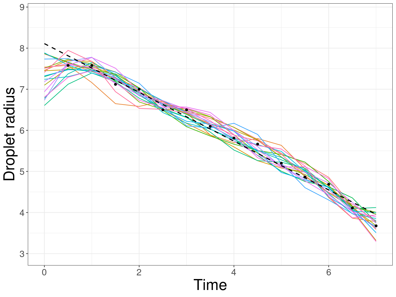
(a) Prior draws

(b) Posterior draws

Figure 2: GP draws of the (a) prior and (b) posterior for the water droplet data. The colored curves represent each draw, the black dots are the observed data and the dashed line is the least squares estimate of the linear model.

Table 1 presents the e-value when testing the original null hypotheses and their pragmatic versions. We provide two choices for $\varepsilon$, one conveying the knowledge of measurement errors ($\varepsilon=0.1606$) and the other being a more restrictive version, evaluating the robustness of the test. Two settings for $\mathcal{X}$ are evaluated, $\mathcal{X}=\{0,0.5,1,\cdots,7\}$ (original setting, discrete uniform) and $t\sim U(0,7)$ (continuous uniform). For $H_{0}^{1}$ and under the finite $\mathcal{X}$, the e-value is high under the informed $Pg(H_{0})$, but low on the other settings. When using the infinite $\mathcal{X}$ instead, the e-value is lowered under $H_{0}$, but raised under the more restrictive $Pg(H_{0})$, evidencing that the FBST in the infinite case is not necessarily a more conservative version of the finite case. Setting $\alpha=0.05$, Fick’s law is rejected only if one ignores the measurement errors of the experiment. For $H_{0}^{2}$, all cases strongly reject the hypothesis, therefore time should remain as a covariate.

Table 1: e-value of $H_{0}$ and $Pg(H_{0})$ under finite and infinite $\mathcal{X}$ for the water droplet experiment.

		Original hypothesis
Assumption on $\boldsymbol{t}$	FBST applied to	$H_{0}^{1}:g(t)=\beta_{0}+\beta_{1}t$	$H_{0}^{2}:g(t)=\beta_{0}$
	$H_{0}$	0.0446	0
$t\in\{0,0.5,1,\cdots,7\}$	$Pg\left(H_{0},d,\frac{0.1606}{3}\right)$	0.0516	0
	$Pg(H_{0},d,0.1606)$	1	0
	$H_{0}$	0.0063	0
$t\sim U(0,7)$	$Pg\left(H_{0},d,\frac{0.1606}{3}\right)$	0.5121	0
	$Pg(H_{0},d,0.1606)$	1	0

Lastly, we present the reasoning behind our choice for $\varepsilon$, with further details found in Lassance et al. (2024). In the original experiment, the radius of the droplets is not obtained directly, but through Stoke’s law instead, i.e.,

$$V_{T}(t)=\frac{g(t)^{2}}{K_{s}}\Longrightarrow g(t)=\sqrt{V_{T}(t)\times K_{s}},$$ (9)

where $V_{T}$ is the terminal velocity and $K_{s}=8.446$. Since the mean velocity ($V_{M}$) was used in (9) instead of $V_{T}$, there are two sources of measurement error: the estimate of $V_{M}$ (maximum error of $\delta=0.14$) and switching $V_{T}$ for $V_{M}$ in (9) (maximum error of $\eta=0.3555$). We conclude that the margin of error of the radius is

$$\epsilon: =\max_{t\in T}|g(t)-y(t)|=\max_{t\in T}\left\{\left|\sqrt{K_{s}V_{T}(t)}-y(t)\right|\right\}$$

$$=\max_{t\in T}\left\{\left|\sqrt{K_{s}(V_{M}(t)-\delta-\eta)}-y(t)\right|,\left|\sqrt{K_{s}(V_{M}(t)+\delta+\eta)}-y(t)\right|\right\}\approx 0.6218.$$

While $\epsilon$ relates to the $l_{\infty}$ distance, Lemma 7 uses the $l_{2}$ distance. To obtain an estimate of the latter from the former, we use Proposition 6.11 of Folland (2013), which implies that

$$\sqrt{\frac{1}{n}\sum_{i=1}^{n}(y(\boldsymbol{x}_{i})-g(\boldsymbol{x}_{i}))^{2}}\leq\sqrt{\frac{1}{n}}\epsilon\Longrightarrow\max_{i\in\{1,2,\cdots,n\}}|y(\boldsymbol{x}_{i})-g(\boldsymbol{x}_{i})|\leq\epsilon,$$

thus $\varepsilon\approx 0.6218/\sqrt{15}\approx 0.1606$.

5 Discussion

Regarding the results of the application (section 4), we believe to have demonstrated the importance of using pragmatic hypotheses whenever reasonable. While choosing $\varepsilon$ is not a simple task in nonparametric settings, there are strategies available for deriving it (Lassance et al., 2024). Furthermore, while the e-value is not a measure of evidence against $H_{0}^{c}$ (De Bragança Pereira et al., 2008), combining it with a pragmatic hypothesis allows one to perform the Generalized FBST (GFBST, (Esteves et al., 2023)), which can discriminate “evidence of absence” from “absence of evidence” along with many other desirable properties.

One of the main limitations of this work is in the strategy of performing variable selection. While the aforementioned GFBST allows for multiple testing without the necessity of correcting $\alpha$, variable selection is only possible through Equation 6 if the linear model hypothesis is not rejected. Therefore, one future research direction is developing tests that evaluate conditional independence without assuming a specific functional form for the relationship between variables.

Conceptualization, all authors; methodology, R.F.L. Lassance and R.B. Stern; software, R.F.L. Lassance; validation, R.F.L. Lassance; formal analysis, R.F.L. Lassance; investigation, J.M. Stern; resources, R.F.L. Lassance; data curation, R.F.L. Lassance; writing—original draft preparation, R.F.L. Lassance; writing—review and editing, all authors; visualization, R.F.L. Lassance; supervision, R.B. Stern and J.M.Stern; project administration, R.B. Stern; funding acquisition, Interinstitutional Graduate Program in Statistics UFSCar-USP. All authors have read and agreed to the published version of the manuscript.

This study was financed in part by the Coordenação de Aperfeiçoamento de Pessoal de Nível Superior - Brasil (CAPES) - Finance Code 001. This research was funded by FAPESP (grants 2019/11321-9 and CEPID CeMEAI 2013/07375-0) and CNPq (grants 309607/2020-5, 422705/2021-7 and PQ 303290/2021-8).

The data and the functions used in this study are available in GitHub at https://github.com/rflassance/lmFBST. These data were derived from the following resource available in the public domain: https://scholarsmine.mst.edu/cgi/viewcontent.cgi?params=/context/masters_theses/article/6294 (page 42, accessed: 05/15/2024).

The authors declare no conflicts of interest. The funders had no role in the design of the study; in the collection, analyses, or interpretation of data; in the writing of the manuscript; or in the decision to publish the results.

Abbreviations The following abbreviations are used in this manuscript:

FBST	Full Bayesian Significance Test
GFBST	Generalized Full Bayesian Significance Test
GP	Gaussian Process
HPD	Highest Posterior Density

no

Appendix A Proofs

Proof of section 3.

The proof is done in parts:

Finite $\mathcal{X}$.

Since $\mathcal{X}$ is finite, Equation 2 is the HPD. Therefore, if $\exists\boldsymbol{\beta}\in\mathbb{R}^{k}$ such that

$$(\boldsymbol{b}(\mathcal{X})\boldsymbol{\beta}-\mu(\mathcal{X}))^{\prime}\Sigma(\mathcal{X},\mathcal{X})^{-1}(\boldsymbol{b}(\mathcal{X})\boldsymbol{\beta}-\mu(\mathcal{X}))\leq q_{(1-\alpha)}(\chi^{2}_{|\mathcal{X}|}),$$ (10)

then the FBST does not reject $H_{0}$. Derivating the left side of (10) in terms of $\boldsymbol{\beta}$, we observe that $\hat{\boldsymbol{\beta}}$ minimizes such expression. ∎

Infinite $\mathcal{X}$.

In this case, the FBST does not reject the hypothesis iff $\exists\boldsymbol{\beta}\in\mathbb{R}^{k}$ such that $RSS(\boldsymbol{b}\times\boldsymbol{\beta})\leq c_{\alpha}$. This is equivalent to not rejecting $H_{0}$ iff

$$\left(\boldsymbol{y}-\boldsymbol{b}(\boldsymbol{X})\left(\boldsymbol{b}(\boldsymbol{X})^{\prime}\boldsymbol{b}(\boldsymbol{X})\right)^{-1}\boldsymbol{b}(\boldsymbol{X})^{\prime}\boldsymbol{y}\right)^{\prime}\left(\boldsymbol{y}-\boldsymbol{b}(\boldsymbol{X})\left(\boldsymbol{b}(\boldsymbol{X})^{\prime}\boldsymbol{b}(\boldsymbol{X})\right)^{-1}\boldsymbol{b}(\boldsymbol{X})^{\prime}\boldsymbol{y}\right)=\boldsymbol{y}^{\prime}\boldsymbol{M}\boldsymbol{y}\leq c_{\alpha},$$

since $\left(\boldsymbol{b}(\boldsymbol{X})^{\prime}\boldsymbol{b}(\boldsymbol{X})\right)^{-1}\boldsymbol{b}(\boldsymbol{X})^{\prime}\boldsymbol{y}$ is the least squares estimate of $\boldsymbol{\beta}$. ∎

∎

Proof of Lemma 7.

The proof is found in Lassance et al. (2024) and is summarised here for completeness. We note that $\mathbb{H}$ is a Hilbert space and that $H_{0}$ is a closed subspace in $\mathbb{H}$ whose basis is $\boldsymbol{b}=(b_{1},b_{2},\cdots,b_{k})$. Setting $(h_{1},h_{2}):=\mathbb{E}_{\boldsymbol{X}}\left[h_{1}(\boldsymbol{X})h_{2}(\boldsymbol{X})\right],\forall h_{1},h_{2}\in\mathbb{H}$, Corollary 5.4 of Brezis (2011) ensures that $\exists\tilde{\boldsymbol{\beta}}_{h}\in\mathbb{R}^{k}:\inf_{h_{0}\in H_{0}}d(h_{0},h)=d(\boldsymbol{b}\times\tilde{\boldsymbol{\beta}}_{h},h)$ characterized by

$$(h-\boldsymbol{b}\times\tilde{\boldsymbol{\beta}}_{h},\boldsymbol{b}\times\boldsymbol{\beta})=\sum_{j=1}^{k}\beta_{j}(h-\boldsymbol{b}\times\tilde{\boldsymbol{\beta}}_{h},b_{j})=0,\quad\forall\boldsymbol{\beta}\in\mathbb{R}^{k},$$

and thus $(h-\boldsymbol{b}\times\tilde{\boldsymbol{\beta}}_{h},b_{j})=0,\forall j\in\{1,2,\cdots,k\}$. Therefore,

$$(h-\boldsymbol{b}\times\tilde{\boldsymbol{\beta}}_{h},b_{j})=(h,b_{j})-\sum_{i=1}^{k}\tilde{\beta}_{h,i}(b_{i},b_{j})=0,\quad\forall j\in\{1,2,\cdots,k\},$$

thus leading to the linear system

$$\left\{\begin{array}[]{c}\sum_{i=1}^{k}\tilde{\beta}_{h,i}(b_{i},b_{1})=(h,b_{1})\\ \sum_{i=1}^{k}\tilde{\beta}_{h,i}(b_{i},b_{2})=(h,b_{2})\\ \vdots\\ \sum_{i=1}^{k}\tilde{\beta}_{h,i}(b_{i},b_{k})=(h,b_{k})\par\end{array}\right.\Longrightarrow A_{\boldsymbol{b}}\times\tilde{\boldsymbol{\beta}}_{h}=\boldsymbol{h}_{\boldsymbol{b}}\Longrightarrow\tilde{\boldsymbol{\beta}}_{h}=A_{\boldsymbol{b}}^{-1}\times\boldsymbol{h}_{\boldsymbol{b}}.$$

∎

Proof of section 3.

The case for the infinite $\mathcal{X}$ follows immediately from Lemma 7. As for when $\mathcal{X}$ is finite, Lemma 7 implies that

$$\tilde{\boldsymbol{\beta}}_{h}=\left(\boldsymbol{b}(\mathcal{X})^{\prime}D_{\mathbb{P}(\mathcal{X})}\boldsymbol{b}(\mathcal{X})\right)\boldsymbol{b}(\mathcal{X})^{\prime}D_{\mathbb{P}(\mathcal{X})}h(\mathcal{X}),$$

and thus

$$d(H_{0},h(\mathcal{X})) =\sqrt{\sum_{\boldsymbol{x}\in\mathcal{X}}\mathbb{P}(\boldsymbol{x})\left(h(\boldsymbol{x})-\boldsymbol{b}(\boldsymbol{x})^{\prime}\tilde{\boldsymbol{\beta}}_{h}\right)^{2}}$$

$$=\sqrt{(h(\mathcal{X})-\boldsymbol{b}(\mathcal{X})\tilde{\boldsymbol{\beta}}_{h})^{\prime}D_{\mathbb{P}(\mathcal{X})}(h(\mathcal{X})-\boldsymbol{b}(\mathcal{X})\tilde{\boldsymbol{\beta}}_{h})}$$

$$=\sqrt{h(\mathcal{X})^{\prime}\boldsymbol{N}h(\mathcal{X})}\leq\varepsilon.$$

Since the HPD is given by Equation 2, the FBST does not reject $Pg(H_{0})$ if and only if

$$\left\{\begin{array}[]{l}h\in\mathbb{H}:d(H_{0},h(\mathcal{X}))=\sqrt{h(\mathcal{X})^{\prime}\boldsymbol{N}h(\mathcal{X})}\leq\varepsilon\\ h\in\mathbb{H}:(h(\boldsymbol{X})-\mu(\mathcal{X}))^{\prime}\Sigma(\mathcal{X},\mathcal{X})^{-1}(h(\mathcal{X})-\mu(\mathcal{X}))\leq q_{1-\alpha}(\chi^{2}_{|\mathcal{X}|})\end{array}\right.$$ (11)

are intersecting ellipsoids. From Proposition 2 of Gilitschenski and Hanebeck (2012), the ellipsoids intersect if and only if

$$\exists s\in(0,1):\quad 1-\mu(\mathcal{X})^{\prime}\left(\frac{\varepsilon^{2}}{1-s}\boldsymbol{N}^{-1}+\frac{1}{s}\Sigma(\mathcal{X},\mathcal{X})q_{(1-\alpha)}(\chi^{2}_{|\mathcal{X}|})\right)\mu(\mathcal{X})<0,$$

thus concluding the proof for the finite case. ∎

References

References

• Kershaw et al. (2001) Kershaw, J.; Kashikura, K.; Zhang, X.; Abe, S.; Kanno, I. Bayesian technique for investigating linearity in event-related BOLD fMRI. Magnetic Resonance in Medicine 2001, 45, 1081–1094.
• Nielsen et al. (2014) Nielsen, J.K.; Christensen, M.G.; Cemgil, A.T.; Jensen, S.H. Bayesian Model Comparison With the g-Prior. IEEE Transactions on Signal Processing 2014, 62, 225–238. https://doi.org/10.1109/TSP.2013.2286776.
• Spiegelhalter et al. (2002) Spiegelhalter, D.J.; Best, N.G.; Carlin, B.P.; Van Der Linde, A. Bayesian measures of model complexity and fit. Journal of the Royal Statistical Society: Series B (Statistical Methodology) 2002, 64, 583–639.
• De Bragança Pereira et al. (2008) De Bragança Pereira, C.A.; Stern, J.M.; Wechsler, S. Can a significance test be genuinely Bayesian? Bayesian Analysis 2008, 3.
• Liu et al. (2024) Liu, Z.; Li, Z.; Wang, J.; He, Y. Full Bayesian Significance Testing for Neural Networks, 2024, [arXiv:stat.ML/2401.13335].
• Pereira and Stern (2020) Pereira, C.A.B.; Stern, J.M. The e-value: a fully Bayesian significance measure for precise statistical hypotheses and its research program. São Paulo Journal of Mathematical Sciences 2020, 16, 566–584.
• Rasmussen and Williams (2006) Rasmussen, C.E.; Williams, C.K.I. Gaussian Processes for Machine Learning; The MIT Press, 2006.
• Esteves et al. (2019) Esteves, L.G.; Izbicki, R.; Stern, J.M.; Stern, R.B. Pragmatic Hypotheses in the Evolution of Science. Entropy 2019, 21.
• Johnson and Wichern (2002) Johnson, R.; Wichern, D. Applied multivariate statistical analysis, 5 ed.; Prentice Hall: Upper Saddle River, NJ, 2002; p. 163.
• Duguid (1969) Duguid, H.A. A study of the evaporation rates of small freely falling water droplets. Master’s thesis, Missouri University of Science and Technology, Rolla, Missouri, USA, 1969.
• Lassance et al. (2024) Lassance, R.F.L.; Izbicki, R.; Stern, R.B. PROTEST: Nonparametric Testing of Hypotheses Enhanced by Experts’ Utility Judgements, 2024, [arXiv:stat.ME/2403.05655].
• Folland (2013) Folland, G. Real Analysis: Modern Techniques and Their Applications; Pure and Applied Mathematics: A Wiley Series of Texts, Monographs and Tracts, Wiley, 2013; p. 186.
• Esteves et al. (2023) Esteves, L.G.; Izbicki, R.; Stern, J.M.; Stern, R.B. Logical coherence in Bayesian simultaneous three-way hypothesis tests. International Journal of Approximate Reasoning 2023, 152, 297–309.
• Brezis (2011) Brezis, H. Functional Analysis, Sobolev Spaces and Partial Differential Equations; Springer New York, 2011.
• Gilitschenski and Hanebeck (2012) Gilitschenski, I.; Hanebeck, U.D. A robust computational test for overlap of two arbitrary-dimensional ellipsoids in fault-detection of Kalman filters. In Proceedings of the 2012 15th International Conference on Information Fusion, 07 2012, pp. 396–401.
\PublishersNote