Can the Near-Horizon Black Hole Memory be detected through Binary Inspirals?

Abstract

The memory effect, in the context of gravitational-waves (GWs), manifests itself in the permanent relative displacement of test masses when they encounter the GWs. A number of works have explored the possibility of detecting the memory when the source and detector are separated by large distances. A special type of memory, arising from BMS symmetries, called “black-hole memory”, has been recently proposed. The black hole memory only manifests itself in the vicinity of its event horizon. Therefore, formally observing it requires placing a GW detector at the horizon of the BH, which prima-facie seems unfeasible. In this work, we describe a toy model that suggests a possible way the black hole memory may be observed, without requiring a human-made detector near the event horizon. The model considers a binary black hole (BBH), emanating GWs observable at cosmological distances, as a proxy for an idealized detector in the vicinity of a supermassive Schwarzschild black hole that is endowed with a supertranslation hair by sending a shock-wave to it. This sudden change affects the geometry near the horizon of the supertranslated black hole and it induces a change in the inspiraling orbital separation (and hence, orbital frequency) of the binary, which in turn imprints itself on the GWs. Using basic GW data analysis tools, we demonstrate that the black hole memory should be observable by a LISA-like space-based detector.

I Introduction

Testing different aspects of gravity has been an active field of research ever since the successful detection of gravitational waves (GWs) with the LIGO detectors in 2015 Abbott et al. (2016, 2020). One of the major issues in gravitational physics is to extract useful information from regions of spacetime where gravity is strong. Black holes are among the most exotic compact objects in the universe having strong gravitational effects near their horizons. GWs generated by violent astrophysical events like the collision of two black holes encode useful information regarding the physics near the horizons.

The LIGO-Virgo (LV) detector network Aasi et al. (2015); Acernese et al. (2015) has detected $\sim 90$ GW events produced by compact binary coalescences (CBCs), across three observing runs (O1, O2, O3) Abbott et al. (2023). The majority of these are binary black hole (BBH) mergers, and have therefore enabled some of the most unique tests of general relativity (GR) in the strong field regime Abbott et al. (2021). These include a model-agnostic test of GR which subtracts out the best matched GR template from the data known to contain the GW signal, and examines if the residual is consistent with noise Abbott et al. (2016); Abbott et al. (2019a); Abbott et al. (2020); an inspiral-merger-ringdown consistency test that checks for consistency between the low and high frequency portions of the GW waveform Ghosh et al. (2016, 2018); a test that looks for deviations in the Post-Newtonian (PN) parameters governing the inspiral evolution of the CBC Blanchet and Sathyaprakash (1994, 1995); Arun et al. (2006a, b); Yunes and Pretorius (2009); Mishra et al. (2010); Li et al. (2012a, b); and propagation tests that compare the speed of GWs with the speed of light Abbott et al. (2019b), as well as signatures of velocity dispersion due to a finite graviton mass Will (1998).

Gravitational memory effect has gained much attention in recent times due to multiple reasons. Memory effect can be understood as the permanent shift in the relative separation of two test detectors placed near null infinity after the passage of GWs Zel’dovich and Polnarev (1974); Braginsky and Thorne (1987):

$$\Delta h_{+,\times}^{mem}=\lim_{t\to\infty}h_{+,\times}(t)-\lim_{t\to-\infty}h_{+,\times}(t)$$

This remarkable feature of spacetime is a genuine test of general relativity. The linear memory appears due to the gravitational radiation generated by binaries executing unbounded (hyperbolic) trajectories and is generally expected to be vanishing for binaries with bound orbits. However, there is another type of memory that originates at the 2.5PN order in the radiative multipoles for quasi-circular and elliptical binary inspirals but contributes at the 0PN order in the waveform Favata (2009). This is in contrast to the hyperbolic, parabolic and radial orbits where this effect occurs at 2.5PN order relative to the leading order (Newtonian) term in the waveform Favata (2011). This is known as non-linear memory or Christodoulou memory Christodoulou (1991); Blanchet and Damour (1992); Thorne (1992). This memory has a simple interpretation: it is the “wave of a wave”, i.e, it arises due to GWs sourced by GWs. This memory signal is expected to be detected by future space-based detectors like LISA (see, e.g., Johnson et al. (2019)).

Recently, an interesting relation between the memory effect and asymptotic symmetries of spacetimes has been established. The asymptotic symmetries are the symmetries that preserve the asymptotic structure of spacetimes. This was first discovered by Bondi-van-der Burg-Metzner and Sachs (BMS) and described in their pioneering works Bondi et al. (1962); Sachs (1962). The group of symmetries recovered near the infinity of an asymptotically flat spacetime is termed as BMS group. In its primitive form, the BMS group contained an infinite dimensional abelian subgroup whose generators are called supertranslations. These are angle dependent translations that generalize the ordinary rigid translations of flat spacetime. Later, the asymptotic group has been extended to accommodate superrotations and can be viewed as conformal symmetries of the celestial sphere at null infinity ($\mathcal{I}^{+}$) Barnich and Troessaert (2010); Barnich and Troessaert (2012).

Supertranslations have an interesting relation with the memory effect. Near null infinity, two test detectors would undergo a shift in their relative position due to the passage of GWs and this can be realized as an action of supertranslation on the boundary data (the physical content of metric at the boundary) Hawking et al. (2016); Strominger and Zhiboedov (2016). This intriguing fact indicates that the detection of the memory effect would be an alternative way to detect supertranslation like symmetries. Since supertranslation (or superrotations) are symmetries of the asymptotic solutions of gravitational theories, they would have their own charges. In fact, there will be an infinite number of conserved charges available due to the supertranslations (or superrotations). These charges reveal that the classical Minkowski vacuum is highly degenerate and different vacua are related by supertranslations Hawking et al. (2017); Strominger (2018). The gravitational memory is now described as a transition between two inequivalent vacua induced by a supertranslation.

Such conservation laws should also be true in the presence of asymptotically flat black holes. However, in this case, the charge conservation requires the black holes should also carry supertranslation (or superrotations) charges or some (soft) ‘hairs’ Hawking et al. (2017); Strominger (2018). In the presence of black holes, the future null infinity ${\mathcal{I}}^{+}$ fails to act as a Cauchy surface. One needs to add the future horizon ${\mathcal{H}}^{+}$ also, and ${\mathcal{I}}^{+}\cup{\mathcal{H}}^{+}$ acts as a Cauchy surface. Therefore, it is desirable to recover the BMS symmetries near the horizon of a black hole in spacetime as well.

BMS symmetries have been recovered near the horizon of a black hole by several theoretical approaches. BMS-like symmetries can be discovered at the null boundaries including black hole horizons by analyzing diffeomorphisms that preserve certain universal structures of these surfaces Chandrasekaran et al. (2018); Ashtekar et al. (2018). In another approach, near-horizon asymptotic symmetries are recovered by preserving the near-horizon asymptotic structures Koga (2001); Donnay et al. (2016a, b).

The emergence of BMS-like symmetries near the horizon of a black hole generates an obvious question: can one find a memory effect similar to what one recovers at null infinity? The answer to this question is affirmative. Memory in the form of a shift in the vacua or solutions upon sending shock-wave on a black hole horizon has been described in Donnay et al. (2018). How near-horizon BMS memory can be imprinted on test observers falling freely near the horizon has also been described in Bhattacharjee et al. (2021). If one considers the symmetries at the black hole horizon, then BMS memory can be defined as the change in certain parameters like expansion, shear related to the null congruences generating the horizon Rahman and Wald (2020); Bhattacharjee et al. (2019); Adami et al. (2021); Sarkar et al. (2022).

Clearly, the existence of such a near-horizon memory or ‘hair’ can only be detected by an idealized observer hovering around the horizon. Can such a memory be recognised from the far region? Particularly, would it be possible to think of a scenario in which the near-horizon memory can show up in future GW detectors? In this article, we propose a toy model that can provide plausible answers to these questions.

II Implantation of memory and its detection

It is apparent that to detect the near-horizon supertranslation memory, one needs to place the detectors close to the horizon. However, detection from a far region would not be possible until the detectors can have some mechanism to communicate with the remote region. To this end, we consider a simplified model and indicate a possible way of obtaining imprints of such near-horizon memory in GWs detectable by the upcoming space-based detectors like LISA.

II.1 The Black Hole Memory

The detection setup uses a toy model in which an eternal Schwarzschild black hole is endowed with a linearised supertranslation hair by throwing some asymmetric shockwave into it as proposed in Hawking et al. (2017); Strominger (2018). This process implants a linearized supertranslation hair to a bald Schwarzschild black hole:

$$g_{\mu\nu}^{Schw}dx^{\mu}dx^{\nu}=-\left(1-{2M\over r}\right)dv^{2}+r^{2}(d\theta^{2}+\sin^{2}\theta d\phi^{2})\,.$$ (1)

The metric with a supertranslation hair is produced by throwing an asymmetric pulse to the black hole at some advanced time $v_{0}$ from $\mathscr{I}^{-}$ with the following energy-momentum density:

$$T_{vv}= \left({\mu+\hat{T}(\theta,\phi)\over 4\pi r^{2}}+{D_{A}\hat{T}^{A}(\theta,\phi)\over 4\pi r^{3}}\right)\delta(v-v_{0}),$$ (2)

$$T_{vA}= {\hat{T}^{A}(\theta,\phi)\over 4\pi r^{2}}\delta(v-v_{0}),$$ (3)

where $D_{A}$ is the covariant derivative on the unit 2-sphere. $\hat{T}^{A}$ satisfies $(D^{2}+2)D_{A}\hat{T}^{A}=-6M\hat{T}$, where $D^{2}$ is the Laplacian on 2-sphere. The above equation can be solved using Green’s function technique to yield the perturbed metric produced by the shock-wave profile Hawking et al. (2017); Strominger (2018). The effect of such a shock-wave is equivalent to the action of a (large) diffeomorphism on the background bald metric:

$$h_{\mu\nu}=\left(\mathcal{L}_{\chi_{f}}g^{Schw}_{\mu\nu}+\dfrac{2\mu}{r}\delta^{v}_{\mu}\delta^{v}_{\nu}\right)\Theta(v-v_{0}).$$ (4)

The BMS Killing vector $\chi_{f}$ acts on the Schwarzschild metric and generates a supertranslated Schwarzschild black hole with a different mass parameter Hawking et al. (2017). The function $f$ is related to the supertranslation symmetry. The shockwave acts as a boundary between a bald black hole and a black hole with supertranslation hair. In the supertranslated phase, $(v>v_{0})$ the metric reads:

$$ds^{2}=-\left(1-{2M\over r}-{MD^{2}f\over r^{2}}\right)dv^{2}+2dvdr$$

$$-dvd\Theta^{A}D_{A}\left(2\left(1-{2M\over r}\right)f+D^{2}f\right)+$$

$$\left(r^{2}\gamma_{AB}+2rD_{A}D_{B}f(\Theta)-r\gamma_{AB}D^{2}f\right)d\Theta^{A}d\Theta^{B},$$ (5)

where $\Theta^{A}$ collectively denotes the angular coordinates $(\theta,\phi)$ on a sphere. This metric is exact in the radial coordinate $r$ but linear in the supertranslational field $f(\theta,\phi)$. The horizon of this supertranslated metric is at $r^{h}_{(f)}=2M+{1\over 2}D^{2}f.$ The transverse components of this metric undergo a shift due to the supertranslation that has been implanted to the horizon of the bald black hole:

$$\Delta h_{AB}=4M\left(D_{A}D_{B}f(\Theta)-{1\over 2}\gamma_{AB}D^{2}f\right).$$ (6)

This change in the transverse part of the metric components gives rise to memory for an observer hovering around the horizon. As the physical degrees of freedom are encoded in the transverse part of the metric, this produces a genuine effect.

BMS-like symmetries can also be recovered near the horizon of a black hole that preserves the near-horizon asymptotic structure. To see this, one may expand the metric in Eq. (II.1) near the horizon by a suitably defined radial coordinate $\rho=r-r^{h}_{(f)}$ and relate the parameters of the near-horizon metric with the implanted supertranslation field Donnay et al. (2016b, 2018). To the leading order in $\rho$ this metric reads:

$$ds^{2}=- {\rho\over 2M}dv^{2}+2dvd\rho-{\rho\over M}D_{A}fd\Theta^{A}dv$$

$$+ (4M^{2}\gamma_{AB}+4MD_{A}D_{B}f)d\Theta^{A}d\Theta^{B}+\mathcal{O}(\rho^{2})\,.$$ (7)

It is not difficult to see that the transverse component of this metric to leading order is identical to (6) except for a term linear in $f$ absorbed in the definition of $\rho$. The bald counterpart of this metric would be obtained by setting $f=0$.

The effect of the near-horizon asymptotic Killing vector $\chi$ (eg. supertranslations) is to preserve the above metric (II.1) but change the background fields. For example, the transverse metric components $\Omega_{AB}$ undergo a change Donnay et al. (2016b, 2018):

$$\delta_{\chi}\Omega_{AB}=4MD_{A}D_{B}f.$$ (8)

The changes induced via horizon supertranslation (or superrotation) are termed as ‘black hole memory effect’ Donnay et al. (2018). The change induced by the shock-wave can be realized as the action of supertranslation and superroation on the near-horizon geometry. One can obtain the charges corresponding to these near-horizon symmetries. The supertranslation and superrotation charges depend upon the field $f$ or its derivatives, and therefore, if we detect $f$ by any mechanism, we detect the supertranslation or the black hole memory.

II.2 A toy detection model

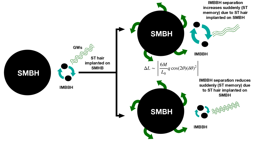
Figure 1: Schematic representation of inspiralling IMBBH source emitting GWs in the vicinity of the horizon of a bald SMBH (on the left). Once the supertranslation (ST) ‘hair’ is attached to the bald SMBH due to some astrophysical shock wave, the proper distance between the components of the IMBBH is changed. The magnitude of the change in separation (ST memory) denoted by $\Delta L$ is given by (11). As the IMBBH separation increases (decreases), the binary will start emitting GWs at a lower (higher) frequency in comparison to the initial configuration (on the left).

Now, we propose a scenario (probe for detection) that might capture this supertranslation memory. Ideally, to detect such a memory one would need to place the detectors near the vicinity of the horizon. Suppose two intermediate-mass black holes (IMBHs) are in the vicinity of a bald supermassive black hole (SMBH) and they act like detectors. The IMBHs initially keep generating GWs which are detectable by LISA. Now suddenly the SMBH (almost instantaneously) gets endowed with a (linear) supertranslation hair by sending a shockwave into it as described above. This sudden effect would change the relative proper distance between the inspiraling IMBHs and would ultimately alter the inspiraling frequency and frequency evolution. Note that the shockwave acts only as an agent that implants the supertranslation hair on the bald SMBH. This is a convenient way to generate a BH state with a (asymptotic) supertranslation field.

We consider the IMBHs to be separated only in the angular directions initially, i.e. they are at the same radial distance from the centre of the hole. After the hair is implanted, the separation between the black holes changes. This can be estimated using local coordinates. We will further assume the supertranslation field to be a function of $\theta$ only. This would reduce the algebra and at the same time offer sufficient insights to the desired investigation. The metric (cf. Eq. II.1) can now be cast in a more explicit form as:

$$ds^{2}= -{1\over 2M}\rho dv^{2}+2dvd\rho-{\rho\over M}\partial_{\theta}fd\theta dv$$

$$+ (4M^{2}d\theta^{2}+4M^{2}\sin\theta^{2}d\phi^{2}+4M\partial_{\theta}^{2}fd\theta^{2}).$$ (9)

Now, let $L_{0}$ be the initial proper distance (angular) between the test bodies (IMBHs). In that case, the separation would only be governed by the bald angular part of the metric. Therefore $L_{0}=4M^{2}\gamma_{AB}d\Theta^{A}d\Theta^{B}.$ After the implantation of the supertranslation memory, the changed distance would be governed by the metric given by Eq. (II.2). If $\Delta L$ is the shift in the separation then a straightforward computation yields:

$$(\Delta L)_{\mathrm{exact}}=\sqrt{L_{0}^{2}-12Mq\cos(2\theta)(\delta\theta)^{2}}-L_{0},$$ (10)

where we have chosen $f(\theta)$ to be equal to the second Legendre Polynomial $f=qP_{2}(\cos\theta).$ $q$ is a parameter that encapsulates the strength of the supertranslation hair Sarkar et al. (2022); Compère and Long (2016). For the case under consideration, $q$ should be small as it is a part of a weak supertranslation field. Practically the initial separation $L_{0}$ should be much greater than the separation induced by the field $f$, so one gets:

$$\Delta L\simeq-{6M\over L_{0}}q\cos(2\theta)(\delta\theta)^{2}.$$ (11)

Here, $\delta\theta$ is the initial azimuthal separation between the objects. The shift in the separation of IMBHs is parametrized by $q$, which will induce a change in the frequency of their inspiraling motion.

II.3 Frequency modulation of the binary

In the previous subsection, we argued that an inspiralling intermediate mass binary black hole (IMBBH) in the vicinity of horizon of supermassive black hole (SMBH) acts as a detector for detecting supertranslation (ST) memory. IMBBH loses energy and angular momentum to GWs which can be observed by Laser Interferometer Space Antenna (LISA). The separation of the binary components $L=2a$ (we call it IMBBH separation) at any instant during inspiral can be related to GW frequency $f$ emitted at that time via Keppler’s law as Peters and Mathews (1963); Peters (1964):

$$a=\left[{(1+z)M_{\mathrm{bin}}\over\pi^{2}f^{2}}\right]^{1/3}\,,$$

where $a$ is the radius of the binary, $z$ is the cosmological redshift of the IMBBH as well as the SMBH, and $M_{\mathrm{bin}}$ is the source-frame total mass of the IMBBH.

Once the supertranslation ‘hair’ is implanted on the central SMBH, the binary separation in IMBBH changes as a result of ST memory as given by Eq. (11). The sudden change in the IMBBH separation leads to a corresponding sudden change in the emitted GW frequency. This instantaneous frequency jump in the GW signal of the IMBBH should be observable. The detection of the ST memory can be quantified by calculating the mismatch between the original GW signal when there is no ST memory and the signal modulated due to the ST memory.

GWs in general relativity have two polarizations i.e., plus $h_{+}$ and cross $h_{\times}$. For quasicircular binaries, the evolution of these polarizations is determined by the intrinsic source parameters ($\vec{\theta}$) i.e., component masses ($m_{1}$, $m_{2}$) and spins ($\vec{\chi}_{1}$, $\vec{\chi}_{2}$); and the extrinsic source parameters ($\vec{\lambda}_{h}$) i.e., luminosity distance $D_{L}$ to the source, inclination angle $\iota$ of the binary with respect to the observer’s line of sight, time $t_{c}$ and phase $\phi_{c}$ at the coalescence. Note that instead of ($m_{1}$, $m_{2}$), it is more natural to use the chirpmass $\mathcal{M}_{c}=(m_{1}m_{2})^{3/5}/(m_{1}+m_{2})^{1/5}$ and mass ratio ${\bf q}=m_{2}/m_{1}$ in the parameter estimation as the shape of gravitational waveform is more sensitive to the chirpmass Cutler and Flanagan (1994a). An interferometric GW detector, such as LISA, records the time-domain strain $h(t;\vec{\theta},\vec{\lambda})$ due to an incoming GW signal, which can be expressed as a linear combination of the plus ($h_{+}$) and cross ($h_{\times}$) polarizations of GWs weighted by the respective antenna responses ($F_{+},F_{\times}$):

$$h_{a}(t;\vec{\theta},\vec{\lambda})=F_{+}(\vec{\lambda}_{F})h_{+}(t;\vec{\theta},\vec{\lambda}_{h})+F_{\times}(\vec{\lambda}_{F})h_{\times}(t;\vec{\theta},\vec{\lambda}_{h})\,,$$ (12)

where $t$ is the detector-frame time, $\vec{\theta}=\{{\mathcal{M}_{c},{\bf q},\vec{\chi}_{1},\vec{\chi}_{2}\}}$, $\vec{\lambda}_{F}=\{{\alpha,\delta,\psi\}}$, $\vec{\lambda}_{h}=\{{D_{L},\iota,t_{c},\phi_{c}\}}$, and $\vec{\lambda}=\vec{\lambda}_{F}\cup\vec{\lambda}_{h}$. $F_{+,\times}(\vec{\lambda}_{F})$ are the antenna pattern functions determined by the extrinsic source parameters $\vec{\lambda}_{F}$ describing the sky-position of the source and polarization angle of the emitted GWs. Sky position of the binary source with respect to the detector is described by right ascension $\alpha$ and declination $\delta$; the polarization angle of the incoming GW is denoted by $\psi$.

Implantation of ST ‘hair’ on the central SMBH leads to a sudden change in the IMBBH separation and a corresponding sudden change in the GW frequency emitted by the binary. This is equivalent to time-shifting the time-domain strain given by Eq. (12) by some amount $\Delta t$ as:

$$h_{b}(t+\Delta t;\vec{\theta},\vec{\lambda})=F_{+}(\vec{\lambda}_{F})h_{+}(t+\Delta t;\vec{\theta},\vec{\lambda}_{h})$$ (13)

$$+F_{\times}(\vec{\lambda}_{F})h_{\times}(t+\Delta t;\vec{\theta},\vec{\lambda}_{h})\,.$$

In the stationary phase approximation (SPA), the Fourier-domain expressions corresponding to Eqs. (12)-(13) can be expressed as Droz et al. (1999):

$$\tilde{h}_{a}(f)=\mathcal{A}e^{i\Psi(f)}=\hat{\mathcal{A}}f^{-7/6}e^{i\Psi(f)}\,,$$ (14)

$$\tilde{h}_{b}(f)=e^{i2\pi f\Delta t}\tilde{h}_{a}(f)\,.$$

Averaging over the inclination angle $\iota$, the amplitude parameter $\hat{\mathcal{A}}$ in the quadrupole approximation is given by Moore et al. (2016); Favata et al. (2022):

$$\hat{\mathcal{A}}=\sqrt{{5\over 24}}\sqrt{{4\over 5}}{\sqrt{\eta}M_{bin}^{5/6}(1+z)^{5/6}\over\pi^{2/3}D_{L}}\,.$$ (15)

Amplitude contains only inclination angle averaging factor ($\sqrt{4/5}$), while the factors due to $60^{\circ}$ angle between LISA arms ($(\sin^{2}60^{\circ})^{-1}$) and sky-polarisation-averaging ($(1/5)^{-1}$) are absorbed into the instrumental noise power spectral density (PSD) of the detector (discussed later in next section). In Eq. ((15)), $M_{\mathrm{bin}}=m_{1}+m_{2}$ is the total binary mass in the source frame with component masses $m_{1}$ and $m_{2}$ , $\eta=m_{1}m_{2}/(m_{1}+m_{2})^{2}={\bf q}/(1+{\bf q})^{2}$ is the symmetric mass ratio. Assuming a flat universe, the luminosity distance-redshift relation is given as Hogg (1999):

$$D_{L}(z)={c\over H_{0}}(1+z)\int_{0}^{z}{dz^{\prime}\over\sqrt{\Omega_{M}(1+z^{\prime})^{3}+\Omega_{\Lambda}}},$$ (16)

with the following cosmological parameters Ade et al. (2016): $H_{0}=67.90\,(\rm{km/s})/\rm{Mpc}$, $\Omega_{M}=0.3065$, and $\Omega_{\Lambda}=0.6935$.

TaylorF2 SPA phase $\Psi(f)$ for circular binaries in the post-Newtonian (PN) theory is expressed as a series in the orbital velocity parameter $v=[\pi M_{\mathrm{bin}}(1+z)f]^{1/3}$ as Blanchet et al. (1995a, b); Kidder (1995); Blanchet (2002); Blanchet et al. (2006); Arun et al. (2009a); Marsat et al. (2013); Mishra et al. (2016):

$$\Psi(f)=2\pi ft_{c}+\phi_{c}+{3\over 128\eta v^{5}}\sum_{k}(\varphi_{k}v^{k}+\varphi_{k}^{\rm log}v^{k}\ln v)\,,$$ (17)

where $t_{c}$ and $\phi_{c}$ are the time and phase of coalescence, respectively. Corrections of order $v^{k}$ correspond to $k/2$-PN order correction relative to the first (0PN/Newtonian) term. The 3.5PN accurate expressions for $(\varphi_{k},\varphi_{k}^{\,log})$ in terms of intrinsic source parameters (masses and spins) are taken from equations in Refs. Arun et al. (2005, 2009a); Buonanno et al. (2009); Wade et al. (2013); Mishra et al. (2016); Blanchet et al. (2023a, b). We consider the binary in quasicircular orbit and components to be nonspinning.

Time-shift $\Delta t$ in Eq. (14) corresponds to the frequency change due to supertranslation memory. Using the energy-balance equation, adiabatic approximation and Kepler’s law, the expression for $\Delta t$ can be expressed at the 0PN (Newtonian) accuracy as Buonanno et al. (2009); Arun et al. (2009a, b); Moore et al. (2016):

$$\Delta t =t(f_{\rm{fi}})-t(f_{\rm{in}})$$

$$={5\over 256}((1+z)\mathcal{M}_{c})^{-5/3}\Big{(}{1\over(\pi f_{\rm{in}})^{8/3}}-{1\over(\pi f_{\rm{fi}})^{8/3}}\Big{)}\,,$$ (18)

where $t(f)$ is the time corresponding to GW frequency $f$, $f_{\rm in}$ and $f_{\rm fi}$ are respectively, the GW frequencies at which binary is emitting before and after supertranslation hair is implanted on the central SMBH and ${\rm\mathcal{M}_{c}}=M_{\rm bin}\eta^{3/5}$ is the chirp mass of the binary. Note that in order to simplify that calculations, we assume the frequency jump due to ST memory from $f_{\rm in}$ to $f_{\rm fi}$ to be discrete.

III Bayesian Parameter Inference

Gravitational wave detector output is the time-domain strain data $d(t)$ which can be decomposed into two components i.e., the detector noise $n(t)$ and the GW signal strain $h(t)$. Given the waveform template $h(t;\vec{\theta},\vec{\lambda})$ representing the GW signal, one needs to estimate the parameters $(\vec{\theta},\vec{\lambda})$ of the GW source. Bayesian parameter estimation invokes Bayes Theorem to estimate the posterior probability distribution $p(\vec{\theta},\vec{\lambda}|d)$ of the signal parameters ($\vec{\theta}$, $\vec{\lambda}$) given the data $d$ and signal model $h(\vec{\theta},\vec{\lambda})$ as:

$$p(\vec{\theta},\vec{\lambda}|d)={\Pi(\vec{\theta},\vec{\lambda})p(d|\vec{\theta},\vec{\lambda})\over p(d)}\,,$$ (19)

where $\Pi(\vec{\theta},\vec{\lambda})$ represents the prior probability distribution, $p(d|\vec{\theta},\vec{\lambda})$ represents the likelihood of the data $d$ and $p(d)$ is the evidence. $p(d)$ can be obtained by marginalizing the likelihood over the signal parameters as:

$$p(d)=\int\Pi(\vec{\theta},\vec{\lambda})p(d|\vec{\theta},\vec{\lambda})d\vec{\theta}d\vec{\lambda}\,.$$ (20)

Assuming the detector noise to be stationary and Gaussian, the likelihood can be written as Cutler and Flanagan (1994b):

$$p(d|\vec{\theta},\vec{\lambda})\propto e^{-{1\over 2}\langle d-h(\vec{\theta},\vec{\lambda})|d-h(\vec{\theta},\vec{\lambda})\rangle}\,,$$

where $d$ is the strain data of the detector and $\langle.|.\rangle$ is the noise-weighted inner product defined as:

$$\langle A|B\rangle=2\int^{\rm{f_{high}}}_{\rm{f_{low}}}{A(f)B^{*}(f)+A^{*}(f)B(f)\over S_{n}(f)}df\,.$$ (21)

Here $f_{\rm low}$, $f_{\rm high}$ are determined by the properties of the binary source, observation time $T_{\rm obs}$ and the detector noise sensitivity. $S_{n}(f)$ is the noise power spectral density (PSD) of the detector. Note that the posteriors $p(\vec{\theta},\vec{\lambda}|d)$ in Eq. (19) are obtained by sampling the high-dimensional (usually fifteen-dimensional for quasicircular binaries) likelihood function approximated as Gaussian.

Assuming the template $\tilde{h}(f)$ to accurately represent the GW signal and considering the detector noise to be stationary and Gaussian, the optimal signal-to-noise ratio (SNR) can expressed as:

$$\rho=\sqrt{4\int^{\infty}_{0}{\left|\tilde{h}(f)\right|^{2}\over S_{n}(f)}df}\,.$$ (22)

Here noise PSD $S_{n}(f)$ of LISA consists of instrumental noise and confusion noise due to the galactic white dwarfs. Eq. (1) of Ref. Babak et al. (2017) provides the instrumental noise PSD and the confusion noise is taken from Eq. (4) of Ref. Mangiagli et al. (2020). The instrumental noise in Ref. Babak et al. (2017) is sky-polarization-averaged and accounts for the $60^{\circ}$ angle between the arms of LISA. We divide the instrumental noise given in Ref. Babak et al. (2017) by a factor of $2$ in order to account for the two effective L-shaped detectors within LISA.

The lower and upper cutoff frequencies ($f_{\rm low}$ and $f_{\rm high}$) used in calculating the integral in Eq. (21) are determined by the detector sensitivity, observation time, and the source properties. The $f_{\rm low}$ is defined as $f_{\rm low}={\rm max}[10^{-4},f_{\rm year}]$, where $f_{\rm year}$ is the GW frequency ${\rm T_{obs}}$ years before the binary emits at the frequency corresponding to the innermost stable circular orbit (ISCO). This frequency, in the quadrupole radiation approximation, is determined by the chirp mass ${\mathcal{M}_{c}}$ and the observation time prior to ISCO $T_{\rm obs}$ as Berti et al. (2005):

$$f_{\rm year}=4.149\times 10^{-5}\left({{\mathcal{M}_{c}}\over 10^{6}M_{\odot}}\right)^{-5/8}\left({T_{\rm obs}\over 1\rm\text{year}}\right)^{-3/8}\,.$$ (23)

We assume $T_{\rm obs}=4$ year in our calculation. The upper cut-off frequency is given by $f_{\rm high}={\rm min}[0.1,f_{\rm ISCO}]$, where $f_{\rm ISCO}=1/({6^{3/2}\pi(1+z)M_{\rm bin}})$ is the GW frequency corresponding to ISCO of a test particle orbiting around a Schwarzschild black hole of mass $M_{\rm bin}$.

We have displayed in Fig. 2, how IMBBH sources of different representative total masses ($10^{3}\,M_{\odot}$, $5\times 10^{3}\,M_{\odot}$, $10^{4}\,M_{\odot}$) at a fixed luminosity distance of $3$ Gpc will evolve in the LISA band. Considering observation time $T_{\rm ob}=4\,{\rm year}$ till ISCO, these sources will inspiral in the LISA band starting from the frequencies corresponding to black markers, merge at frequencies corresponding to magenta markers.

Let $f_{\rm ref}$ be the reference frequency to which the binary has evolved, when the ST hair is implanted on the SMBH. We choose this frequency to be $4\,{\rm mHz}$, which is close to the high sensitivity regime of LISA. Indeed, the binaries are still $375$ days, $26$ days and $8$ days (shown by purple markers), respectively, away from reaching their respective ISCOs.

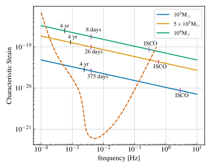
Figure 2: The evolution of the characteristic (dimensionless) strain Moore et al. (2015) (inclination-averaged) of three representative IMBBH sources with equal-mass components (solid lines) shown in comparison to the characteristic (dimensionless) strain corresponding to the noise PSD of LISA (dashed curve). Luminosity distance of the IMBBH sources is fixed at $3$ Gpc. The magenta markers denote the GW strain and GW frequency of the IMBBH sources at the corresponding ISCO. The purple markers at $f_{\rm ref}=4\,{\rm mHz}$ denote the time till ISCO. The black markers represent the characteristic strain, and GW frequency, $T_{\rm obs}=4$ years before ISCO.

IV Model selection

In the context of this work, the GW signal emitted by the IMBBH can be modelled in two ways – with ($\tilde{h}_{b}(f)$) and without ($\tilde{h}_{a}(f)$) ST memory. In order to determine whether one model (say $\tilde{h}_{b}(f)$) is preferred over another model (say $\tilde{h}_{b}(f)$), we need to do a comparative analysis which involves the calculation of Bayes factor. Bayes factor is defined as the ratio of the two marginalized likelihoods (evidences) calculated under each of the two hypotheses – the hypothesis $\mathcal{H}_{b}$($\mathcal{H}_{a}$) that the GW signal in the data $d$ contains (doesn’t contain) the supertranslation (ST) memory imprint. This factor can be expressed as:

$$\mathcal{B}^{b}_{a}={p(d|\mathcal{H}_{b})\over p(d|\mathcal{H}_{a})}={\int p(\vec{\theta}|\mathcal{H}_{b})p(d|\vec{\theta},\mathcal{H}_{b})d\vec{\theta}\over\int p(\vec{\theta}|\mathcal{H}_{a})p(d|\vec{\theta},\mathcal{H}_{a})d\vec{\theta}}\,.$$ (24)

In the limit of high SNR, the above expression for Bayes factor can be simplified and written in terms of optimal SNR and fitting factor (FF) as Cornish et al. (2011); Vallisneri (2012):

$$\text{ln}\mathcal{B}^{b}_{a}\approx(1-\text{FF})\rho^{2}\,,$$ (25)

where ${\rm FF}$ is defined as the match between the two waveform models $\tilde{h}_{b}(f)$ ($\tilde{h}_{a}(f)$) under two different hypotheses $\mathcal{H}_{b}$ ($\mathcal{H}_{a}$) maximized over the intrinsic source parameters $\vec{\theta}$ and can be written as Apostolatos (1995); Vallisneri (2012):

$$\text{FF}\equiv\langle\tilde{h}_{a}(f)|\tilde{h}_{b}(f)\rangle_{\text{max}(\vec{\theta})}\,.$$ (26)

The match $\mathcal{M}$ between two waveform models $\tilde{h}_{a}(f)$ and $\tilde{h}_{b}(f)$ quantifies the overlap between the two models and is defined as:

$$\mathcal{M}={\langle\tilde{h}_{a}(f)|\tilde{h}_{b}(f)\rangle\over(\langle\tilde{h}_{a}(f)|\tilde{h}_{a}(f)\rangle\langle\tilde{h}_{b}(f)|\tilde{h}_{b}(f)\rangle)^{1/2}}\,.$$ (27)

The denominator of the above expression can be simplified using Eq. (14) as:

$$\langle\tilde{h}_{a}(f)|\tilde{h}_{a}(f)\rangle=\langle\tilde{h}_{b}(f)|\tilde{h}_{b}(f)\rangle=\left|\tilde{h}_{a}(f)\right|^{2}\,.$$ (28)

Using Eq. (14), $\tilde{h}_{a}(f)=\tilde{h}_{b}(f)$ only for $f<f_{\rm ref}$ just before the ST hair is implanted on the central SMBH (i.e., $\Delta t=0$). Hence, using Eq. (21), the numerator of Eq. (27) can be written as a sum of two parts corresponding to $f<f_{\rm ref}$ and $f>f_{\rm ref}$ as:

$$\langle\tilde{h}_{a}(f)|\tilde{h}_{b}(f)\rangle =4\int^{f_{\rm ref}}_{f_{\rm low}}{\left|\tilde{h}_{a}(f)\right|^{2}\over S_{n}(f)}df$$ (29)

$$+2\int^{f_{\rm high}}_{f_{\rm ref}}{2\left|\tilde{h}_{a}(f)\right|^{2}\cos({2\pi f\Delta t})\over S_{n}(f)}df$$

Here $f_{\rm{ref}}$ is the GW frequency at which the binary is emitting corresponding to the time the ST memory is imparted to the binary.

V Results

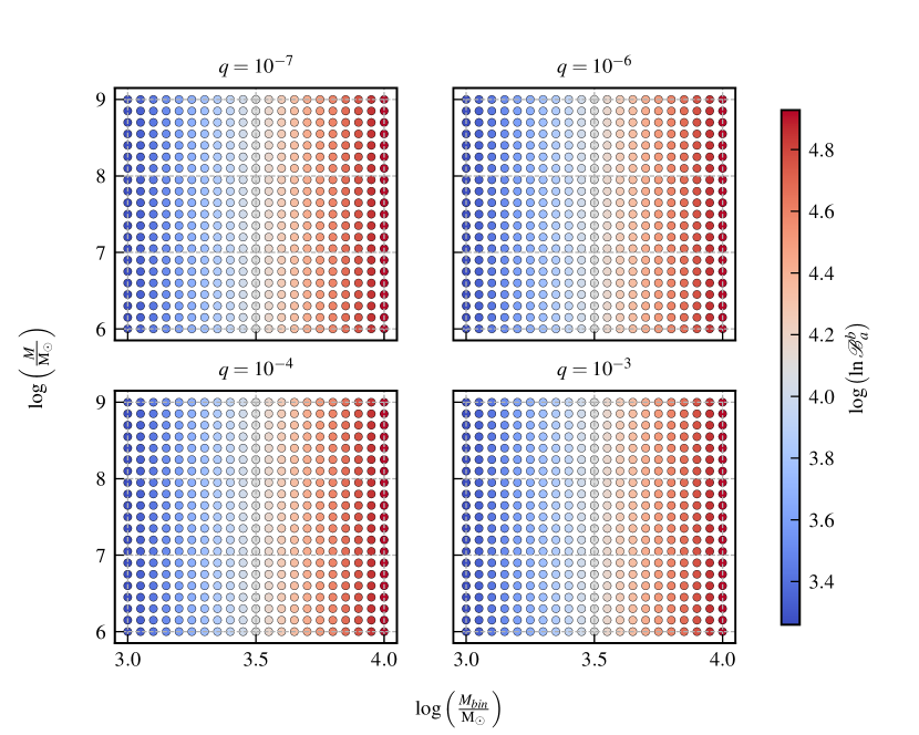
Figure 3: The ${\rm\log}({\rm ln\mathcal{B}}^{\rm b}_{\rm a})$ to determine whether the model of GWs with (b)/without (a) imprints of black hole memory is preferred, is shown in the color scale. These Bayes factors are evaluated on a grid of total binary mass (${\rm\log}(M_{\rm bin}/M_{\odot})$) and mass of supermassive black hole (${\rm\log}(M/M_{\odot})$). GW frequency corresponding to the time when supertranslation hair is imparted to SMBH is fixed at $f_{\rm ref}=4\,{\rm mHz}$. Supertranslation charge $q$ is varied across the different panels shown. This figure corresponds to the case when ST memory leads to an increase (corresponding to $\cos(2\theta)=-1$ ) in binary separation.

Having introduced the waveform models in Sec. II.3, Bayesian inference in Sec. III and model comparison in Sec. IV, we discuss the results here. We construct a $21\times 21$ grid uniform-in-log of the total mass $M_{\rm{bin}}$ of IMBBH and uniform-in-log of the mass $M$ of SMBH. The masses of the IMBBH and SMBH are restricted to the ranges $10^{3}\mbox{--}10^{4}\,\rm{M_{\odot}}$ and $10^{6}\mbox{--}10^{9}\,\rm{M_{\odot}}$, respectively. We fix the mass-ratio at q $=1$ (corresponding to $m_{1}=m_{2}$). The binary components of the IMBBH source are assumed to be nonspinning. The luminosity distance $D_{L}$ of the IMBBH source (and SMBH as well) is chosen to be $3$ Gpc. We calculate the SNRs of the simulated sources within the LISA band and find that the SNRs fall in the range ($50-300$). These SNRs are high enough to validate the high-SNR approximation used in Eq. (25) of Sec. IV for simplifying the calculation of the Bayes factor Vallisneri (2008); Cokelaer (2008); Rodriguez et al. (2013).

The supertranslation charge $q$ appearing in Eq. (11) is chosen from a set of discrete values: ($10^{-7}$, $10^{-6}$, $10^{-4}$, $10^{-3}$) and the reference GW frequency $f_{\rm{ref}}$, corresponding to the time at which ST memory is imparted to the binary, is chosen to be $4\,\rm{mHz}$. This corresponds to the bottom of the noise PSD “bucket” (Fig. 2) where the LISA detector is the most sensitive.

To show that the GW signal prefers the model with ST memory over the model without ST memory, we calculate Bayes-factor for all the simulated sources using the parameter setup discussed. Figure 3 (corresponding to $\cos 2\theta=-1$ in Eq. (11)) shows the scatter-plot for Bayes-factor in the $M-M_{\rm{bin}}$ plane. The different panels in the figure pertain to different values of supertranslation charge as mentioned. We see that Log-Bayes-Factor increases with increasing total mass $M_{\rm{bin}}$ of the IMBBH which is due to an increase in the optimal SNR of the GW signal. Given a total mass $M_{\rm{bin}}$ of the binary, Log-Bayes-Factor shows weak dependence on mass $M$ of SMBH. Increasing the value ST charge $q$ increases the strength of supertranslation memory as shown in different panels of Fig. 3. When the ST charge $q$ is higher, we get higher Log-Bayes-Factor for given masses $M_{\rm{bin}}$, $M$ of the binary and SMBH, respectively.

For all chosen values of ST charge $q$, Log-Bayes-Factor values are in the range $10^{3}\mbox{--}10^{5}$ as shown in different panels of Fig. 3. This shows that the near-horizon ST memory can be confidently detected in the LISA band. We also computed Log-Bayes-Factor corresponding to $\cos 2\theta=1$ and sky-averaged value of $\cos 2\theta$ in Eq. (11). We do not find any significant difference (at order of magnitude) compared to $\cos 2\theta=-1$.

VI Conclusion

We have presented, as a proof of principle, a toy model to detect the horizon supertranslation memory. The set up involves an IMBBH emitting GWs detectable by LISA, in the vicinity of an SMBH suddenly endowed with the memory, which acts as a proxy for a detector. The sudden change in the spacetime metric surrounding the SMBH produces a sharp change in the frequency and frequency evolution of the GWs, which can be exploited to identify the occurrence of this memory. We refer the reader to Goncharov et al. (2024) for other possible mechanisms that could enable the detection of BMS-symmetries through GW memory in next generation (XG) detectors.

The detection scheme outlined here, as a proof of principle, possesses caveats that would need to be addressed to realistically detect the black hole memory.

• The source of the shockwave in a realistic astrophysical scenario is unknown, although many interesting results have been reported in theoretical studies of asymptotic symmetries and memory effects using this model Hawking et al. (2016, 2017); Strominger (2018); Donnay et al. (2016a, 2018); Bhattacharjee et al. (2021); Sarkar et al. (2022); Donnay et al. (2016b); Chu and Koyama (2018).

• The change in the proper length of the IMBBHs is measured using a near-horizon metric. Thus, ideally, ST should be recovered near the horizon. On the other hand, realistically, the binary system should at least be outside the ISCO of the SMBH. The ISCO for the ST Schwarzschild black hole is not in general close to its horizon. For a bald Schwarzschild black hole, it is at $3$ times its Schwarzschild radius, and this distance may not be ideal for the detection scenario considered in this work. Of course, the ISCO lies very close to the horizon of a rapidly spinning Kerr black hole. Such rapidly spinning SMBHs are indeed expected in nature Reynolds (2015). Nevertheless, we have also considered the metric (II.1), proposed by the authors Hawking et al. (2017), which is valid for any finite radial distance from the center of the SMBH, and calculated the memory and the corresponding Log-Bayes-Factors. These values remain similar to what’s presented in Figure 3 at order of magnitude even if we place the detectors outside the ISCO of a supertranslated SMBH.

• The GW waveform used for the non-spinning IMBBH does not account for environmental effects. The presence of the SMBH would modulate the waveform due to effects such as line of sight acceleration (see, e.g., Vijaykumar et al. (2023)), aberration (see, e.g., Torres-Orjuela et al. (2020)) and lensing (see, e.g., D’Orazio and Loeb (2020)). In fact, to fully capture all the effects of SMBH on the GWs will require ray-tracing. Nevertheless, we expect the sudden change in the metric producing a discrete jump in the frequency of the IMBBH’s GWs to be detectable over and above all the additional modulations incurred due to the presence of the SMBH.

• The rate of IMBBH mergers, or for that matter, CBCs in general in the vicinity of SMBHs, remains uncertain. Some works in the literature have proposed the existence of migration traps in disks of active galactic nuclei (AGNs). These traps could foster CBC mergers, some of which could lie very close to the ISCO of the central SMBH (see, e.g., Peng and Chen (2021)).

Another plausible mechanism to detect the black hole memory involves extreme mass ratio inspirals (EMRIs). In this case, a stellar mass black hole orbits an SMBH, which is suddenly endowed with a “radial” (instead of “azimuthal” as considered in this work) ST hair, causing the orbital radius of the EMRI to suddenly increase, thus modulating it. We expect the signature of such an ST memory also to be detectable. We plan to calculate this radial ST hair and the corresponding change in the metric, as well as its signature on the EMRI GWs, to provide some insights on this alternative detection setup.

References

- Abbott et al. (2016) B. P. Abbott et al. (LIGO Scientific Collaboration and Virgo Collaboration), Phys. Rev. Lett. 116, 061102 (2016), URL https://link.aps.org/doi/10.1103/PhysRevLett.116.061102.
- Abbott et al. (2020) R. Abbott et al. (LIGO Scientific Collaboration and Virgo Collaboration), Phys. Rev. Lett. 125, 101102 (2020), URL https://link.aps.org/doi/10.1103/PhysRevLett.125.101102.
- Aasi et al. (2015) J. Aasi et al. (LIGO Scientific), Class. Quant. Grav. 32, 074001 (2015), eprint 1411.4547.
- Acernese et al. (2015) F. Acernese et al. (Virgo), Class. Quant. Grav. 32, 024001 (2015), eprint 1408.3978.
- Abbott et al. (2023) R. Abbott et al. (KAGRA, VIRGO, LIGO Scientific), Phys. Rev. X 13, 041039 (2023), eprint 2111.03606.
- Abbott et al. (2021) R. Abbott et al. (LIGO Scientific, VIRGO, KAGRA) (2021), eprint 2112.06861.
- Abbott et al. (2016) B. P. Abbott et al. (LIGO Scientific, Virgo), Phys. Rev. Lett. 116, 221101 (2016), [Erratum: Phys.Rev.Lett. 121, 129902 (2018)], eprint 1602.03841.
- Abbott et al. (2019a) B. P. Abbott et al. (LIGO Scientific, Virgo), Phys. Rev. D 100, 104036 (2019a), eprint 1903.04467.
- Abbott et al. (2020) R. Abbott et al. (LIGO Scientific, Virgo), Astrophys. J. Lett. 900, L13 (2020), eprint 2009.01190.
- Ghosh et al. (2016) A. Ghosh et al., Phys. Rev. D 94, 021101 (2016), eprint 1602.02453.
- Ghosh et al. (2018) A. Ghosh, N. K. Johnson-Mcdaniel, A. Ghosh, C. K. Mishra, P. Ajith, W. Del Pozzo, C. P. L. Berry, A. B. Nielsen, and L. London, Class. Quant. Grav. 35, 014002 (2018), eprint 1704.06784.
- Blanchet and Sathyaprakash (1994) L. Blanchet and B. S. Sathyaprakash, Classical and Quantum Gravity 11, 2807 (1994).
- Blanchet and Sathyaprakash (1995) L. Blanchet and B. S. Sathyaprakash, Phys. Rev. Lett. 74, 1067 (1995).
- Arun et al. (2006a) K. G. Arun, B. R. Iyer, M. S. S. Qusailah, and B. S. Sathyaprakash, Phys. Rev. D 74, 024006 (2006a), eprint gr-qc/0604067.
- Arun et al. (2006b) K. G. Arun, B. R. Iyer, M. S. S. Qusailah, and B. S. Sathyaprakash, Class. Quant. Grav. 23, L37 (2006b), eprint gr-qc/0604018.
- Yunes and Pretorius (2009) N. Yunes and F. Pretorius, Phys. Rev. D 80, 122003 (2009), eprint 0909.3328.
- Mishra et al. (2010) C. K. Mishra, K. G. Arun, B. R. Iyer, and B. S. Sathyaprakash, Phys. Rev. D 82, 064010 (2010), eprint 1005.0304.
- Li et al. (2012a) T. G. F. Li, W. Del Pozzo, S. Vitale, C. Van Den Broeck, M. Agathos, J. Veitch, K. Grover, T. Sidery, R. Sturani, and A. Vecchio, Phys. Rev. D 85, 082003 (2012a), eprint 1110.0530.
- Li et al. (2012b) T. G. F. Li, W. Del Pozzo, S. Vitale, C. Van Den Broeck, M. Agathos, J. Veitch, K. Grover, T. Sidery, R. Sturani, and A. Vecchio, J. Phys. Conf. Ser. 363, 012028 (2012b), eprint 1111.5274.
- Abbott et al. (2019b) B. P. Abbott et al. (LIGO Scientific, Virgo), Phys. Rev. Lett. 123, 011102 (2019b), eprint 1811.00364.
- Will (1998) C. M. Will, Phys. Rev. D 57, 2061 (1998), eprint gr-qc/9709011.
- Zel’dovich and Polnarev (1974) Y. B. Zel’dovich and A. G. Polnarev, SvA 18, 17 (1974).
- Braginsky and Thorne (1987) V. B. Braginsky and K. S. Thorne, Nature (London) 327, 123 (1987).
- Favata (2009) M. Favata, Phys. Rev. D 80, 024002 (2009), eprint 0812.0069.
- Favata (2011) M. Favata, Phys. Rev. D 84, 124013 (2011), eprint 1108.3121.
- Christodoulou (1991) D. Christodoulou, Phys. Rev. Lett. 67, 1486 (1991).
- Blanchet and Damour (1992) L. Blanchet and T. Damour, Phys. Rev. D 46, 4304 (1992), URL https://link.aps.org/doi/10.1103/PhysRevD.46.4304.
- Thorne (1992) K. S. Thorne, Phys. Rev. D 45, 520 (1992), URL https://link.aps.org/doi/10.1103/PhysRevD.45.520.
- Johnson et al. (2019) A. D. Johnson, S. J. Kapadia, A. Osborne, A. Hixon, and D. Kennefick, Phys. Rev. D 99, 044045 (2019), eprint 1810.09563.
- Bondi et al. (1962) H. Bondi, M. G. J. Van der Burg, and A. W. K. Metzner, Proceedings of the Royal Society of London. Series A. Mathematical and Physical Sciences 269, 21 (1962), URL https://royalsocietypublishing.org/doi/abs/10.1098/rspa.1962.0161.
- Sachs (1962) R. Sachs, Phys. Rev. 128, 2851 (1962), URL https://link.aps.org/doi/10.1103/PhysRev.128.2851.
- Barnich and Troessaert (2010) G. Barnich and C. Troessaert, Phys. Rev. Lett. 105, 111103 (2010), URL https://link.aps.org/doi/10.1103/PhysRevLett.105.111103.
- Barnich and Troessaert (2012) G. Barnich and C. Troessaert, Supertranslations call for superrotations (2012), eprint 1102.4632.
- Hawking et al. (2016) S. W. Hawking, M. J. Perry, and A. Strominger, Phys. Rev. Lett. 116, 231301 (2016), URL https://link.aps.org/doi/10.1103/PhysRevLett.116.231301.
- Strominger and Zhiboedov (2016) A. Strominger and A. Zhiboedov, Journal of High Energy Physics 2016, 86 (2016), ISSN 1029-8479, URL https://doi.org/10.1007/JHEP01(2016)086.
- Hawking et al. (2017) S. W. Hawking, M. J. Perry, and A. Strominger, Journal of High Energy Physics 2017, 161 (2017), ISSN 1029-8479, URL https://doi.org/10.1007/JHEP05(2017)161.
- Strominger (2018) A. Strominger, Lectures on the infrared structure of gravity and gauge theory (2018), eprint 1703.05448.
- Chandrasekaran et al. (2018) V. Chandrasekaran, É. É. Flanagan, and K. Prabhu, Journal of High Energy Physics 2018, 125 (2018), ISSN 1029-8479, URL https://doi.org/10.1007/JHEP11(2018)125.
- Ashtekar et al. (2018) A. Ashtekar, M. Campiglia, and A. Laddha, General Relativity and Gravitation 50, 140 (2018), ISSN 1572-9532, URL https://doi.org/10.1007/s10714-018-2464-3.
- Koga (2001) J.-i. Koga, Physical Review D 64 (2001), ISSN 1089-4918, URL http://dx.doi.org/10.1103/PhysRevD.64.124012.
- Donnay et al. (2016a) L. Donnay, G. Giribet, H. A. González, and M. Pino, Phys. Rev. Lett. 116, 091101 (2016a), URL https://link.aps.org/doi/10.1103/PhysRevLett.116.091101.
- Donnay et al. (2016b) L. Donnay, G. Giribet, H. A. González, and M. Pino, Journal of High Energy Physics 2016, 100 (2016b), ISSN 1029-8479, URL https://doi.org/10.1007/JHEP09(2016)100.
- Blau and O’Loughlin (2016) M. Blau and M. O’Loughlin, Journal of High Energy Physics 2016, 29 (2016), ISSN 1029-8479, URL https://doi.org/10.1007/JHEP03(2016)029.
- Bhattacharjee and Bhattacharyya (2018) S. Bhattacharjee and A. Bhattacharyya, Phys. Rev. D 98, 104009 (2018), URL https://link.aps.org/doi/10.1103/PhysRevD.98.104009.
- Donnay et al. (2018) L. Donnay, G. Giribet, H. A. González, and A. Puhm, Phys. Rev. D 98, 124016 (2018), URL https://link.aps.org/doi/10.1103/PhysRevD.98.124016.
- Bhattacharjee et al. (2021) S. Bhattacharjee, S. Kumar, and A. Bhattacharyya, Journal of High Energy Physics 2021, 134 (2021), ISSN 1029-8479, URL https://doi.org/10.1007/JHEP03(2021)134.
- Rahman and Wald (2020) A. A. Rahman and R. M. Wald, Phys. Rev. D 101, 124010 (2020), URL https://link.aps.org/doi/10.1103/PhysRevD.101.124010.
- Bhattacharjee et al. (2019) S. Bhattacharjee, S. Kumar, and A. Bhattacharyya, Phys. Rev. D 100, 084010 (2019), URL https://link.aps.org/doi/10.1103/PhysRevD.100.084010.
- Adami et al. (2021) H. Adami, D. Grumiller, M. M. Sheikh-Jabbari, V. Taghiloo, H. Yavartanoo, and C. Zwikel, JHEP 11, 155 (2021), eprint 2110.04218.
- Sarkar et al. (2022) S. Sarkar, S. Kumar, and S. Bhattacharjee, Phys. Rev. D 105, 084001 (2022), eprint 2110.03547.
- Compère and Long (2016) G. Compère and J. Long, Journal of High Energy Physics 2016, 137 (2016), ISSN 1029-8479, URL https://doi.org/10.1007/JHEP07(2016)137.
- Peters and Mathews (1963) P. C. Peters and J. Mathews, Phys. Rev. 131, 435 (1963).
- Peters (1964) P. C. Peters, Physical Review 136, B1224 (1964).
- Cutler and Flanagan (1994a) C. Cutler and E. E. Flanagan, Phys. Rev. D 49, 2658 (1994a), eprint gr-qc/9402014.
- Droz et al. (1999) S. Droz, D. J. Knapp, E. Poisson, and B. J. Owen, Phys. Rev. D 59, 124016 (1999), eprint arXiv:gr-qc/9901076.
- Moore et al. (2016) B. Moore, M. Favata, K. G. Arun, and C. K. Mishra, Phys. Rev. D 93, 124061 (2016), eprint arXiv:1605.00304 [gr-qc].
- Favata et al. (2022) M. Favata, C. Kim, K. G. Arun, J. Kim, and H. W. Lee, Phys. Rev. D 105, 023003 (2022), eprint 2108.05861.
- Hogg (1999) D. W. Hogg (1999), eprint arXiv:astro-ph/9905116.
- Ade et al. (2016) P. A. R. Ade et al. (Planck), Astron. Astrophys. 594, A13 (2016), eprint arXiv:1502.01589 [astro-ph.CO].
- Blanchet et al. (1995a) L. Blanchet, T. Damour, B. R. Iyer, C. M. Will, and A. G. Wiseman, Phys. Rev. Lett. 74, 3515 (1995a), eprint arXiv:gr-qc/9501027.
- Blanchet et al. (1995b) L. Blanchet, T. Damour, and B. R. Iyer, Phys. Rev. D 51, 5360 (1995b), [Erratum: Phys.Rev.D 54, 1860 (1996)], eprint arXiv:gr-qc/9501029.
- Kidder (1995) L. E. Kidder, Phys. Rev. D 52, 821 (1995), eprint arXiv:gr-qc/9506022.
- Blanchet (2002) L. Blanchet, Living Rev. Rel. 5, 3 (2002), eprint arXiv:gr-qc/0202016.
- Blanchet et al. (2006) L. Blanchet, A. Buonanno, and G. Faye, Phys. Rev. D 74, 104034 (2006), [Erratum: Phys.Rev.D 75, 049903 (2007), Erratum: Phys.Rev.D 81, 089901 (2010)], eprint arXiv:gr-qc/0605140.
- Arun et al. (2009a) K. G. Arun, A. Buonanno, G. Faye, and E. Ochsner, Phys. Rev. D 79, 104023 (2009a), [Erratum: Phys.Rev.D 84, 049901 (2011)], eprint arXiv:0810.5336 [gr-qc].
- Marsat et al. (2013) S. Marsat, A. Bohe, G. Faye, and L. Blanchet, Classical Quantum Gravity 30, 055007 (2013), eprint arXiv:1210.4143 [gr-qc].
- Mishra et al. (2016) C. K. Mishra, A. Kela, K. G. Arun, and G. Faye, Phys. Rev. D 93, 084054 (2016), eprint arXiv:1601.05588 [gr-qc].
- Arun et al. (2005) K. G. Arun, B. R. Iyer, B. S. Sathyaprakash, and P. A. Sundararajan, Phys. Rev. D 71, 084008 (2005), [Erratum: Phys.Rev.D 72, 069903 (2005)], eprint arXiv:gr-qc/0411146.
- Buonanno et al. (2009) A. Buonanno, B. Iyer, E. Ochsner, Y. Pan, and B. S. Sathyaprakash, Phys. Rev. D 80, 084043 (2009), eprint arXiv:0907.0700 [gr-qc].
- Wade et al. (2013) M. Wade, J. D. E. Creighton, E. Ochsner, and A. B. Nielsen, Phys. Rev. D 88, 083002 (2013), eprint arXiv:1306.3901 [gr-qc].
- Blanchet et al. (2023a) L. Blanchet, G. Faye, Q. Henry, F. Larrouturou, and D. Trestini (2023a), eprint arXiv:2304.11185 [gr-qc].
- Blanchet et al. (2023b) L. Blanchet, G. Faye, Q. Henry, F. Larrouturou, and D. Trestini (2023b), eprint arXiv:2304.11186 [gr-qc].
- Arun et al. (2009b) K. G. Arun, L. Blanchet, B. R. Iyer, and S. Sinha, Phys. Rev. D 80, 124018 (2009b), eprint arXiv:0908.3854 [gr-qc].
- Cutler and Flanagan (1994b) C. Cutler and E. E. Flanagan, Phys. Rev. D 49, 2658 (1994b), eprint arXiv:gr-qc/9402014.
- Babak et al. (2017) S. Babak, J. Gair, A. Sesana, E. Barausse, C. F. Sopuerta, C. P. Berry, E. Berti, P. Amaro-Seoane, A. Petiteau, and A. Klein, Physical Review D 95, 103012 (2017).
- Mangiagli et al. (2020) A. Mangiagli, A. Klein, M. Bonetti, M. L. Katz, A. Sesana, M. Volonteri, M. Colpi, S. Marsat, and S. Babak, Physical Review D 102, 084056 (2020).
- Berti et al. (2005) E. Berti, A. Buonanno, and C. M. Will, Phys. Rev. D 71, 084025 (2005), eprint arXiv:gr-qc/0411129.
- Moore et al. (2015) C. J. Moore, R. H. Cole, and C. P. L. Berry, Class. Quant. Grav. 32, 015014 (2015), eprint 1408.0740.
- Cornish et al. (2011) N. Cornish, L. Sampson, N. Yunes, and F. Pretorius, Phys. Rev. D 84, 062003 (2011), eprint 1105.2088.
- Vallisneri (2012) M. Vallisneri, Phys. Rev. D 86, 082001 (2012), eprint 1207.4759.
- Apostolatos (1995) T. A. Apostolatos, Phys. Rev. D 52, 605 (1995), URL https://link.aps.org/doi/10.1103/PhysRevD.52.605.
- Vallisneri (2008) M. Vallisneri, Phys. Rev. D 77, 042001 (2008), eprint gr-qc/0703086.
- Cokelaer (2008) T. Cokelaer, Classical and Quantum Gravity 25, 184007 (2008).
- Rodriguez et al. (2013) C. L. Rodriguez, B. Farr, W. M. Farr, and I. Mandel, Phys. Rev. D 88, 084013 (2013), eprint arXiv:1308.1397 [astro-ph.IM].
- Goncharov et al. (2024) B. Goncharov, L. Donnay, and J. Harms, Inferring fundamental spacetime symmetries with gravitational-wave memory: from LISA to the Einstein Telescope (2024), eprint arXiv:2310.10718 [gr-qc].
- Chu and Koyama (2018) C.-S. Chu and Y. Koyama, JHEP 04, 056 (2018), eprint 1801.03658.
- Reynolds (2015) C. S. Reynolds, The Physics of Accretion onto Black Holes pp. 277–294 (2015).
- Vijaykumar et al. (2023) A. Vijaykumar, A. Tiwari, S. J. Kapadia, K. G. Arun, and P. Ajith, Astrophys. J. 954, 105 (2023), eprint 2302.09651.
- Torres-Orjuela et al. (2020) A. Torres-Orjuela, X. Chen, and P. Amaro-Seoane, Phys. Rev. D 101, 083028 (2020), eprint 2001.00721.
- D’Orazio and Loeb (2020) D. J. D’Orazio and A. Loeb, Phys. Rev. D 101, 083031 (2020), eprint 1910.02966.
- Peng and Chen (2021) P. Peng and X. Chen, MNRAS 505, 1324 (2021), eprint 2104.07685.