Stabilising nonlinear travelling waves in pipe flow using time-delayed feedback

Abstract

We demonstrate the first successful non-invasive stabilisation of nonlinear travelling waves in a straight circular pipe using time-delayed feedback control (TDF). The main novelty in this work is in the application of a “multiple time-delayed feedback” (MTDF) approach, where several control terms are required to attenuate a broad range of unstable eigenfrequencies. We implement a gradient descent method to dynamically adjust the gain functions, $G_{i}(t),$ in order to reduce the need for tuning a high dimensional parameter space. We consider the effect of the control terms via an approximate linear analysis and a frequency-domain analysis, which justifies the choice of MTDF parameters. By using an adaptive approach to setting the control gains, we advocate for a broad range of MTDF terms which are then free to find their own stabilising amplitudes for a given target solution, thereby removing trial and error when the instability of the target solution is unknown a’priori. This also enables travelling waves to be stabilised from generic turbulent states and with speculative starting parameters.

1 Introduction

In this study, we consider the incompressible Navier–Stokes equations as a high-dimensional dynamical system, where simple invariant solutions, or exact coherent structures (ECSs), can be considered key building blocks of the spatiotemporal chaos (see, e.g., Kawahara et al., 2012; Graham & Floryan, 2021). Exact coherent structures take the form of equilibria, relative equilibria (or travelling waves), periodic orbits, and relative periodic orbits. The study of ECS has shed light on the origin of turbulence statistics (Chandler & Kerswell, 2013; Lucas & Kerswell, 2015; Page et al., 2024), the physical mechanisms that play a role in sustaining turbulence (van Veen et al., 2006; Lucas & Kerswell, 2017; Yasuda et al., 2019; Graham & Floryan, 2021), subcritical transition to turbulence (Skufca et al., 2006; Kreilos & Eckhardt, 2012), mixing and layer formation in stratified flow (Lucas & Caulfield, 2017; Lucas et al., 2017), pattern formation in convection (Beaume et al., 2011; Reetz & Schneider, 2020) amongst other applications. The fundamental objective is to be able to describe a turbulent flow by using ECSs as a reduced order description and as a simple way to predict its statistics. ECSs in various fluid flows have been successfully isolated using homotopy (Nagata, 1990), bisection (Itano & Toh, 2001; Duguet et al., 2008b), and recurrent flow analysis (Viswanath, 2007, 2009; Chandler & Kerswell, 2013). Newton-Krylov methods have proved the most successful and efficient methods for converging these unstable states, however, as the Reynolds number or system size are increased, and the flow becomes increasingly disordered, well-conditioned guesses become harder to identify. Recently several authors have attempted to overcome this shortcoming by attempting to minimise some functional using variational methods (Farazmand, 2016; Azimi et al., 2020) or automatic differentiation (Page et al., 2021), or using convolutional autoencoders (Page et al., 2023). Here, our approach will be to instead control the underlying ECSs and simply timestep onto them. We will develop a time-delayed feedback control method to stabilise travelling waves from turbulence in pipe flow. This method serves to complement existing methods to find ECSs and provides new insight into flow control in general. A relatively rich literature on ECSs in pipe flow exists, with many travelling wave solutions (Faisst & Eckhardt, 2003; Wedin & Kerswell, 2004; Pringle et al., 2009; Viswanath, 2009; Willis et al., 2013; Ozcakir et al., 2016, 2019) and relative periodic solutions (Budanur et al., 2017; Duguet et al., 2008a) reported. Moreover experimental observations suggest that these solutions to the governing equations, with idealised boundary conditions, do have relevance to real-world applications (Hof et al., 2006). Feedback control has been used to great effect by Willis et al. (2017) to obtain ‘edge-states’ in pipe flow but it remains to be seen if more generalised control methods can obtain other ECSs. For these reasons pipe flow is an excellent candidate system in which to test and develop this control approach.

The method of time-delayed feedback control, sometimes called Pyragas control (Pyragas, 1992), is a well-known approach for stabilising invariant solutions in chaotic systems and has been used to great effect in a variety of dynamical systems (Ushakov et al., 2004; Popovych et al., 2005; Yamasue & Hikihara, 2006; Stich et al., 2013; Lüthje et al., 2001) . A finite-dimensional dynamical system with state vector $\bm{X}(t)$ can be expressed as

$$\frac{\mathrm{d}\bm{X}}{\mathrm{d}t}=\bm{f}(\bm{X}(t),t;\bm{p})+\bm{F}\>,$$ (1)

in our case the vector field $\bm{f}$ is given by the discretised Navier-Stokes equation with parameters $\bm{p}$, and we denote $\bm{F}$ as the time-delayed feedback ‘force’;

$$\bm{F}(t)=G(t)[\bm{X}(t-\tau)-\bm{X}(t)]\>,$$ (2)

where $\bm{X}(t)$ and $\bm{X}(t-\tau)$ are the current state vector and the time delayed state vector, with delay period $\tau.$ $G(t)$ is the control gain, which in general could be some matrix (thereby coupling feedback between degrees of freedom) but here is a function of time only. Note that when a time periodic state with period $\tau,$ or a time-independent state, is stabilised successfully, the control force (2) will decay exponentially towards zero. This can only occur if the stabilised state is itself a solution of the uncontrolled system, so that TDF is considered to be a non-invasive control method. One reason for the lack of application of TDF in fluid systems is likely due to the so-called “odd-number” limitation. This claims that states with an odd-number of unstable Floquet multipliers are unable to be stabilised by this method (Just et al., 1999; Nakajima & Ueda, 1998b). Nakajima (1997) explains the issue from a bifurcation perspective; the non-invasive feature means that the number of solutions of period $\tau$ cannot vary with $G,$ however any stabilisation requires a change of stability and hence bifurcation. Such a bifurcation cannot, therefore, be of pitchfork or saddle-node type (changing $\tau$-period solutions), and so must involve the crossing of a complex conjugate pair of exponents in a Hopf or period-doubling bifurcation. There have been numerous studies offering resolutions to this issue, including forcing oscillation of the unstable manifold through $G$ (Schuster & Stemmler, 1997; Flunkert & Schöll, 2011), an ‘act-and-wait’ approach (Pyragas & Pyragas, 2019), using symmetries (Nakajima & Ueda, 1998a; Lucas & Yasuda, 2022) and by counter example (Fiedler et al., 2011; Sieber, 2016).

Shaabani-Ardali et al. (2017) report the application of Pyragas control to suppress vortex pairing in a periodically forced jet. This work approaches the control method as a frequency damping technique; filtering out non-harmonic frequencies, leaving only $\tau$ behind. Here the odd-number issue can be viewed as a zero-mode limit where there is no incipient frequency to damp.

Recently, Lucas & Yasuda (2022) applied this method to two-dimensional Kolmogorov flow turbulence, validating the stabilisation of the base flow via linear stability analysis and showing successful stabilisation of several equilibria and travelling waves. This was achieved by including the symmetries of the target solutions into the control force. In many examples, including the stabilisation of the laminar solution, this was an effective means to avoid the odd-number problem (not too dissimilar to, but different from, the “half-period” approach in Nakajima & Ueda (1998a)). An adaptive, gradient descent, approach is also used to obtain the relative translations of travelling waves so that the method can be successful without any foreknowledge of the ECS.

Our main objective in this paper is to present an improved method for using TDF to stabilise nonlinear traveling waves in pipe turbulence, where the flows are more physically relevant, more unstable and have more spatial complexity.

The vast majority of TDF research has been devoted to investigating the linear stability of a target solution, it being a necessary property for successful stabilisation (Nakajima, 1997). However, this is not a sufficient condition as successful practical stabilisation can also depend on the initial conditions. In high dimensional systems it would be advantageous to design the control to also maximise the basin of attraction of the stabilised state. Furthermore it will be necessary for the TDF control to stabilise several unstable directions, each with differing eigenfrequencies, without knowing what these frequencies are before initiating the control. To achieve this, we develop an adaptive version of the multi-frequency damping TDF control method (Akervik et al., 2006; Shaabani-Ardali et al., 2017), i.e., multiple time-delayed feedback (MTDF), where several TDF terms are used. One drawback of the MTDF approach is the need to optimise a separate control gain for each delay period applied. In order to avoid a trial-and-error sampling of this high-dimensional parameter space, we apply a gradient descent method (Lehnert et al., 2011) to evolve each $G$ towards their stabilising values.

This paper is organised as follows. In § 2, we describe the governing equations for pipe flow with the control force, the numerical method, the continuous and discrete symmetries, and define relevant flow measures. In § 3, after introducing single time-delayed feedback for pipe flow and the adaptive translation method, we demonstrate some successful cases stabilising an unstable travelling wave at low Reynolds number. We predict the behaviour of TDF by using an approximate linear stability analysis and control theory, in such a way identifying the optimal control parameters for this solution. In § 4, we introduce multiple delayed feedback control (MTDF) and demonstrate its effectiveness in stabilising more highly unstable states and analyse it’s behaviour from the frequency damping perspective. In § 5, we demonstrate successful stabilisation of travelling waves from relatively high Reynolds number turbulence, using MTDF alongside the optimisation methods for gains and translations.

2 Numerical formulation

2.1 Pipe flow with time-delayed feedback

We consider the incompressible, viscous flow in straight, circular, pressure-driven pipes. We non-dimensionalise the governing equations with the Hagen–Poiseuille (HP) centreline speed, $U_{\mathrm{cl}}$, and pipe radius, $R$. This yields the dimensionless incompressible Navier–Stokes equations:

$$\frac{\partial}{\partial t}\bm{U}+(\bm{U}\cdot\nabla)\bm{U}=-\nabla p+\frac{4}{Re}(1+\beta)\hat{\bm{z}}+\frac{1}{Re}\nabla^{2}\bm{U}+\bm{F},$$ (3)

$$\nabla\cdot\bm{U}=0\>,$$ (4)

with the no-slip condition on the boundary,

$$\bm{U}(1,\theta,z)=\bm{0}\>.$$ (5)

Here, $\bm{U}$ is the three-dimensional velocity vector, with $p$ the perturbation pressure away from the imposed pressure gradient; $Re=RU_{\mathrm{cl}}/\nu$ is the Reynolds number, $\nu$ is the kinematic viscosity of fluid, and time $t$ is defined in the unit of $R/U_{\mathrm{cl}}$. The dimensionless variable, $\beta(t)$, is the fractional pressure gradient needed to maintain a constant mass flux in the streamwise direction, in addition to the one required to drive the laminar HP flow. $\bm{F}$ is an external body force that, here, will include the time-delayed feedback control terms. We consider equations (3) and (4) in cylindrical-polar coordinates $(r,\theta,z)$, where $r$ is the radius position, $\theta$ is the azimuthal angle position, and $z$ is the streamwise (axial) position.

With the aforementioned non-dimensionalisation, the laminar Hagen–Poiseuille flow is expressed as

$$\bm{U}_{\mathrm{HP}}(r)=(1-r^{2})\hat{\bm{z}}\>,$$ (6)

where $\hat{\bm{z}}$ is the unit vector in the streamwise direction. The laminar HP flow is found at low Reynolds numbers and is linearly stable even at very large (or possibly infinite) Reynolds numbers (Salwen et al., 1980; Meseguer & Trefethen, 2003). Fundamental studies of pipe flow consider either driving with a constant mass flux (Darbyshire & Mullin, 2006; Duguet et al., 2008a; Willis et al., 2013) or a constant pressure gradient (Wedin & Kerswell, 2004; Shimizu & Kida, 2009). In what follows we will seek comparisons with ECSs enumerated in Willis et al. (2013); therefore we choose to use the same constant mass flux formulation, requiring $\beta(t)$ to be obtained dynamically through the following equation,

$$1+\beta(t)=\frac{D(t)}{D_{\mathrm{lam}}}\>,$$ (7)

where $D(t)$ is the total energy dissipation rate for the flow, and $D_{\mathrm{lam}}$ is that for the laminar flow (see § 2.3 for the definitions).

We solve the above system using the open-source code openpipeflow (Willis, 2017) which allows the relatively easy implementation of our control terms. Our computational domain is periodic in both azimuthal and streamwise directions, and the streamwise length of the periodic pipe is $L=\pi/\alpha$, e.g., with $\alpha=1.25$ corresponding to $L\approx 2.5D$. The fluctuating velocity, $\bm{u}$ ($=\bm{U}-\bm{U}_{\mathrm{HP}}$), and the fluctuating pressure, $p$, are both expanded in discrete Fourier series in the streamwise and azimuthal directions. Spatial derivatives with respect to $r$ are evaluated based on a 9-point finite differences stencil with a non-uniform mesh, for which 1st/2nd order derivatives are calculated to 8th/7th order (Willis, 2017). With these spatial discretisation schemes, $\bm{u}$ is expressed as

$$\bm{u}(r_{n},\theta,z,t)=\sum_{|k|<K}\sum_{|m|<M}\widetilde{\bm{u}}_{km}(r_{n},t)\mathrm{e}^{i(\alpha kz+m\theta)}$$ (8)

where $\widetilde{\bm{u}}$ is the Fourier coefficient of $\bm{u}.$ $r_{n}$ ($n=1\ldots N$) denotes the radial grid points (non-uniformly distributed on [0, 1]) and $k$ and $m$ are the streamwise and azimuthal wavenumbers respectively, with $K$ and $M$ the de-aliasing cutoff (see Willis, 2017). The resolution of a given calculation is described by a vector $(N,M,K)$ and is adjusted until the energy in the spectral coefficients drops by at least 5 and usually 6 decades. Time-stepping is via a second-order predictor-corrector scheme, with Euler predictor for the non-linear terms and Crank-Nicolson for the viscous diffusion.

2.2 Continuous and discrete symmetries

The equations of pipe flow are invariant under continuous translations in $z$

$$\mathcal{T}_{z}(s_{z})[u_{r},u_{\theta},u_{z},p](r,\theta,z)\rightarrow[u_{r},u_{\theta},u_{z},p](r,\theta,z+s_{z})\>,$$ (9)

continuous rotations in $\theta,$

$$\mathcal{T}_{\theta}(s_{\theta})[u_{r},u_{\theta},u_{z},p](r,\theta,z)\rightarrow[u_{r},u_{\theta},u_{z},p](r,\theta+s_{\theta},z)\>,$$ (10)

and reflections about $\theta=0$

$$\sigma[u_{r},u_{\theta},u_{z},p](r,\theta,z)\rightarrow[u_{r},-u_{\theta},u_{z},p](r,-\theta,z)\>,$$ (11)

Following the approach by Willis et al. (2013), we will restrict our investigations to dynamics restricted to the ‘shift-and-reflect’ symmetry subspace, $S=\sigma\mathcal{T}_{z}\left(\frac{L}{2}\right)$,

$$S[u_{r},u_{\theta},u_{z},p](r,\theta,z)\rightarrow[u_{r},-u_{\theta},u_{z},p](r,-\theta,z-L_{z}/2)\>,$$ (12)

and the discrete ‘rotate-and-reflect’ symmetry $Z_{m_{p}}=\sigma\mathcal{T}_{\theta}\left(\frac{\pi}{m_{p}}\right)$,

$$Z_{m_{p}}[u_{r},u_{\theta},u_{z},p](r,\theta,z)\rightarrow[u_{r},-u_{\theta},u_{z},p](r,\pi/m_{p}-\theta,z)\>.$$ (13)

Note $m_{p}=1$ denotes azimuthal periodicity (the full space), and $m_{p}$-fold rotational symmetry is enforced for $m_{p}\geq 2$ (Wedin & Kerswell, 2004; Pringle et al., 2009; Willis et al., 2013). By imposing $S$ the flow is ‘pinned’ in $\theta$ and continuous rotations are prohibited. This means that our solutions are only permitted to travel in the streamwise direction due to $\mathcal{T}_{z}.$

2.3 Flow measures

In order to monitor the system behaviour, we consider the integrated quantities from the energy budget equation

$$\frac{\mathrm{d}E}{\mathrm{d}t}=I-D+I_{\mathrm{TDF}}\>,$$ (14)

where $E$ is the total kinetic energy, $I$ is the total energy input due to the imposed pressure gradient and $D$ is the total energy dissipation

$$E\coloneqq\frac{1}{2}\int|\bm{U}|^{2}\mathrm{d}V\>,\,I\coloneqq\oint p\bm{U}\cdot\bm{n}\mathrm{d}S\>,\,D\coloneqq\frac{1}{Re}\int|\nabla\times\bm{U}|^{2}\mathrm{d}V\>.$$ (15)

$I_{\mathrm{TDF}}$ is the total energy input due to feedback force $\bm{F}$,

$$I_{\mathrm{TDF}}\coloneqq\int\bm{U}\cdot\bm{F}\mathrm{d}V\>.$$ (16)

For the laminar state, $I_{\mathrm{TDF}}=0$ and the values of $E$, $I$, and $D$ can be computed, respectively, by

$$E_{\mathrm{lam}}\coloneqq\frac{1}{2}\int|\bm{U}_{\mathrm{HP}}|^{2}\mathrm{d}V\>,\,I_{\mathrm{lam}}\coloneqq\oint p\bm{U}_{\mathrm{HP}}\cdot\bm{n}\mathrm{d}S\>,\,D_{\mathrm{lam}}\coloneqq\frac{1}{Re}\int|\nabla\times\bm{U}_{\mathrm{HP}}|^{2}\mathrm{d}V\>.$$ (17)

3 Time-delayed feedback

3.1 Formulation

In this section we outline the application of the time-delayed feedback control (2) to the pipe. In order to effectively stabilise travelling wave solutions, the delayed state must be translated by a streamwise shift $s_{z}$ in relation to the phase speed, $c_{z}$ such that $c_{z}=\frac{s_{z}}{\tau}$ for a given time delay $\tau.$ Using the translation operator (9), the most basic form of TDF force in pipe flow may be formulated as

$$\bm{F}_{\mathrm{TDF}}(r,\theta,z,t)=G(t)[\mathcal{T}_{z}(s_{z})\bm{u}(r,\theta,z,t-\tau)-\bm{u}(r,\theta,z,t)]\>,$$ (18)

where $\tau$ is the delay period, and $G(t)$ is the gain. Note the gain here is a simple scalar function of time, but it may itself be an operator (matrix) or spatially inhomogenous. In the full space one may also wish to apply a rotation $\mathcal{T}_{\theta}.$

In order to avoid a discontinuity propagating through the solution when the control is initiated, we set $G(t)$ using the following sigmoid function:

$$G(t)=\begin{cases}\frac{G^{\mathrm{max}}}{1+\exp[a(b+t_{s}-t)]}\>,&\qquad t>t_{s}\\ 0&\qquad t\leq t_{s}.\end{cases}$$ (19)

Here, $t_{s}$ is start time (the time TDF is initiated), $G^{\mathrm{max}}$ is the maximum gain, and $a$ determines the slope of $G(t)$ and the half-height time, $t_{h}=t_{s}+b,$ set by $b,$ is when $G(t_{h})=G^{\mathrm{max}}/2$.

The value of the translation, $s_{z},$ for successful stabilisation will be, in general, unknown in advance, so we require a method to evolve $s_{z}$ towards the required value. We implement the adaptive method developed in Lucas & Yasuda (2022). This method allows $s_{z}$ to vary via gradient descent by solving an ordinary differential equation

$$\frac{\mathrm{d}s_{z}}{\mathrm{d}t}=\gamma_{s}\delta s_{z},$$ (20)

where $\gamma_{s}$ is a parameter controlling the speed of the descent and $\delta s_{z}$ is, near a travelling state, an estimate of the streamwise translation remaining between the current state and the delayed and translated state. Specifically, $\delta s_{z}$ is computed as

$$\delta s_{z}=s_{z}^{\mathrm{est}}-s_{z}\>,$$ (21)

where $s_{z}^{\mathrm{est}}$ is a streamwise translation that is dynamically estimated. Here, $s_{z}^{\mathrm{est}}$ can be computed via the time series of $c_{z}(t)$ such that

$$s_{z}^{\mathrm{est}}(t;\tau)=\int_{t-\tau}^{t}c_{z}(t^{\prime})\mathrm{d}t^{\prime}\>.$$ (22)

We can compute $c_{z}(t)$ using complex phase rotations such that

$$c_{z}(t)=\frac{1}{N_{\mathrm{e}}}\sum_{k=\pm 1}\sum_{m=\pm 1}\sum_{n=1}^{N-1}\frac{1}{i\alpha k\Delta t}\arg\bigg{[}\frac{\widetilde{u}_{km}(r_{n},t)}{\widetilde{u}_{km}(r_{n},t-\Delta t)}\bigg{]}$$ (23)

where $N_{\mathrm{e}}=4(N-2)$ is the number of the elements in the above summation and the wall points ($n=N$) are excluded. Note that $c_{z}(t)$ is considered an average phase speed over one time step, $\Delta t$, in the streamwise direction. We solve the ODE (20) while computing $s_{z}^{\mathrm{est}}$ using (22) alongside the DNS with a second-order Adams-Bashforth time stepping scheme.

As will be seen in the later sections, using long time delays can be essential in successful stabilisation of unstable travelling waves in a straight circular pipe. Computing estimated translations using (22) is slightly different from the original version in Lucas & Yasuda (2022). The current version is found to perform better than the original when encountering long delays.

sol.	$Re$	$\alpha$	$E/E_{\mathrm{lam}}$	$D/D_{\mathrm{lam}}$	$c_{z}$	$m_{p}$	sym.	$\mu_{i}>0$	$\textrm{max}(\mu_{i})$	$\textrm{min}(\omega_{i})$ s.t. $\mu_{i}>0$
ML	$2400$	1.25	0.88662	1.6970	0.71049	2	$S$,$Z_{2}$	1c	0.0061985	0.018295
							$S$	1r+3c	0.0676	0.018295
UB	$2400$	1.25	0.85273	2.5102	0.64924	2	$S$,$Z_{2}$	3c	0.056285	0.32393
							$S$	9c	0.10689	0.048437
							–	2r+17c	0.10751	0.048437
	$3700$	1.25	0.84822	2.4866	0.65056	2	$S$,$Z_{2}$	6c	0.077546	0.19076
S2U	$2400$	1.25	0.89383	1.4695	0.64763	2	$S$	1c	0.014152	0.13040
							–	1r+2c	0.014152	0.12385
N3	$2400$	2.5	0.83421	3.0283	0.59508	3	$S$,$Z_{3}$	–	–	–
							$S$	1r+6c	0.091251	0.084125
							–	1r + 11c	0.091250	0.084125
N4U	$2500$	1.7	0.84927	3.2796	0.52575	4	$S$,$Z_{4}$	4c	0.24623	0.10674
							$S$	14c	0.24623	0.047864
							–	1r + 28c	0.24623	$9.9240\times 10^{-4}$

Table 1: Table summarising the properties of all travelling waves studied in this paper. $Re=RU_{\mathrm{cl}}/\nu$ is the Reynolds number, $\alpha$ is the streamwise wavenumber, $E$ is the total kinetic energy, $D$ is the total energy dissipation rate, $c_{z}$ is the streamwise phase velocity, $\lambda_{i}=\mu_{i}\pm\mathrm{i}\omega_{i}$ are the eigenvalues of the solutions.

3.2 Validation – Stabilising weakly unstable solutions

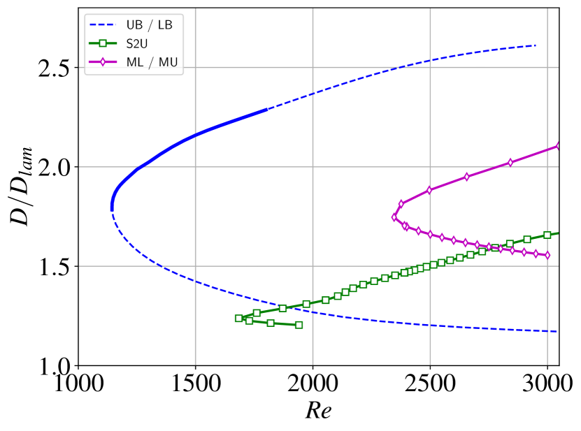
Figure 1: Bifurcation diagram showing solution branches for flows with $\alpha=1.25$.

(a)

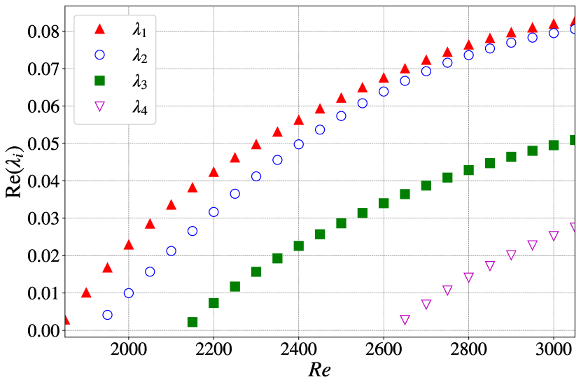
(b)

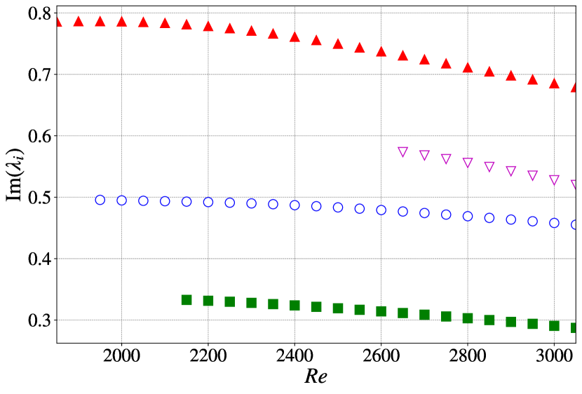
Figure 2: The $Re$-dependence of leading eigenvalues of UB solution. (a) Real part and (b) imaginary part of unstable complex eigenvalues. No purely real eigenvalue exists; thus the “odd-number limitation” is not encountered.

(a)

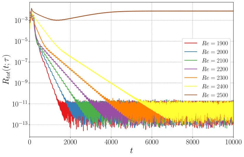
(b)

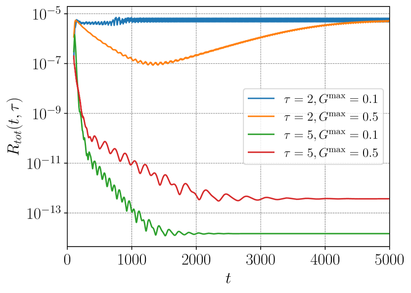
Figure 3: Time series in the relative residual, $R_{\mathrm{tot}}(t;\tau)$ for attempted TDF stabilisation of UB. (a) shows $Re=1900$,$2000$,$2100$,$2200$,$2300$,$2400$,$2500$ for TDF parameters $\tau=2$ and $G^{\max}=0.5,$ stabilisation fails for $Re>2400$. Right plot (b) shows the $Re=2500$ case with $\tau=2,\,5$ and $G^{\max}=0.1$ and 0.5, demonstrating consistency with the linear analysis. The simulations are initiated with UB at each Reynolds number. Note that recording $R_{\mathrm{tot}}(t;\tau)$ initiates at $t=\tau$.

In the absence of any simpler solutions to use for validation (the laminar HP flow is linearly stable at least up to $Re=10^{7}$, see Meseguer & Trefethen (2003)), we attempt to stabilise known unstable travelling waves (Willis et al., 2013) at low $Re$ first. For the parameter values of $\alpha=1.25$ ($L_{z}\approx 5R$) and $Re=2400$, we are able to stabilise the travelling waves ML, UB, S2U in their respective symmetric subspace (see table 1). These travelling waves have only complex unstable eigenvalues at $\alpha=1.25$ and $Re=2400$ and in their symmetry subspaces, meaning that the odd-number issue is not applicable, or rather is avoided by projection into those subspaces (see Lucas & Yasuda, 2022, for a discussion).

In order to investigate the effectiveness of TDF as the stability of a target solution changes, we concentrate on the UB solution and vary $Re,$ returning to the other solutions in § 5.3. Figure 1 shows the bifurcation diagram with the continuation of the UB solution branch (blue) as a function of $Re$ (alongside ML and S2U). This is generated numerically using the Newton–GMRES–hookstep method (Viswanath, 2007, 2009) packaged with the openpipeflow code (Willis, 2017). This confirms that UB originates in a saddle-node bifurcation at $Re\approx 1150$. On increasing $Re$, the stable upper branch (solid line in figure 1) of UB becomes unstable via a supercritical Hopf bifurcation at $Re\approx 1800$ (unstable solution in dashed blue).

In figure 2 we plot the real and imaginary parts of the complex growth rates of the UB solution which demonstrates the expected increase in instability. A sequence of further bifurcations are observed and new unstable directions are formed as more eigenvalues cross the real axis. The solution has only complex eigenvalues at least up to $Re=3050$, therefore it is free from the odd-number limitation (Nakajima, 1997).

Armed with this stability information we attempt to stabilise UB at various $Re$ using TDF. The initial condition is UB such that $\bm{U}(r,\theta,z,0)=\bm{U}_{\mathsf{UB}}$. We set $t_{s}=10$ such that the trajectory is still close to the UB solution when TDF is activated, avoiding the need to consider if our initial condition falls inside the basin of attraction for now. In this sense this section verifies a necessary condition for stabilisation and we will investigate more generic initial conditions later.

In order to quantify the size of the TDF force term, we define the relative residual, $R_{\mathrm{tot}}$, between the current state and the translated and delayed state, as

$$R_{\mathrm{tot}}=\frac{\|\mathcal{T}_{z}(s_{z})\bm{U}(r,\theta,z,t-\tau)-\bm{U}(r,\theta,z,t)\|_{2}}{\|\bm{U}(r,\theta,z,t)\|_{2}}$$ (24)

where $\|\bm{A}\|_{2}=\sqrt{\frac{1}{2}\int\bm{A}\cdot\bm{A}\mathrm{d}V.}$ Figure 3 shows time series in $R_{\mathrm{tot}}$ for seven Reynolds numbers, $Re=1900$, 2000, 2100, 2200, 2300, 2400, 2500, with $\tau=2,$ $G^{\mathrm{max}}=0.5,$ $\gamma_{s}=0.1,$ $t_{s}=10,$ $a=0.1,$ $b=100.$ At $Re=1900$, stabilisation of UB is achieved quickly such that $R_{\mathrm{tot}}$ has decreased to $O(10^{-12})$ by $t=2000$. As expected the rate of attraction of the travelling wave decreases as $Re$ increases with all other parameters held fixed.

At $Re=2500$, stabilisation is unsuccessful; even by increasing $G^{\mathrm{max}}$ we are unable to stabilise the UB state at this $Re.$ It turns out that the growth rate is not the key quantity preventing stabilisation in this case, and neither is it the appearance of an odd-numbered eigenvalue (in contrast to the findings in Lucas & Yasuda (2022)). UB at $Re=2500$ has three unstable eigenfrequencies, which are decreasing as a function of $Re;$ it is these values which fall outside the domain of stabilisation of our method. In the next subsection, we analyse the TDF control from the perspective of “frequency damping” (Akervik et al., 2006; Shaabani-Ardali et al., 2017) and linear stability analysis.

3.3 Frequency damping and linear stability with TDF

Predicting the outcome of TDF in these scenarios is difficult due to the relatively high dimension of the unstable manifold (of the uncontrolled solution) and the highly nonlinear nature of the solution. Nevertheless we can approximate the effect of the TDF terms on the unstable part of the eigenvalue spectrum. Starting from equation (1)-(2), assuming $\bm{X}=\bar{\bm{X}}+\bm{v}e^{\lambda t},$ with $\bar{\bm{X}}$ a steady state solution to (1), assuming $G$ is now constant and linearising in the usual way results in the modified eigenvalue problem

$$\lambda\bm{v}=\mathcal{J}\bm{v}+G\bm{v}\left(e^{-\lambda\tau}-1\right),$$ (25)

with eigenvalue $\lambda,$ eigenvector $\bm{v}$ and $\mathcal{J}$ being the Jacobian of $\bm{f}.$ The eigenvalue problem is now transcendental and so requires some numerical root searching to obtain the eigenvalues. Lucas & Yasuda (2022) tackled this difficulty by assuming $|\lambda\tau|\ll 1$ and expanding the exponential, however we are unable to make this assumption here. Moreover, root-searching for $\lambda$ in the full problem, i.e. some numerical linearisation of (3), would be impractical. Instead we create a “synthetic” $\mathcal{J},$ which we design to have the same unstable eigenvalues as the uncontrolled solution, and some randomly chosen eigenvectors. At $Re=2500$, with three pairs of unstable, complex eigenvalues, this amounts to a 6 dimensional real-valued system. We can then solve the transcendental characteristic equation numerically with a simple Newton search to obtain all of the roots and hence eigenvalues. This procedure is able to predict well the effect of TDF on the UB solution; at the parameters shown in figure 3 the analysis finds that the largest eigenvalue crosses the imaginary axis at $Re\approx 2450.$ Moreover it is sufficiently efficient that we can explore the $(G,\tau)$ parameter space. Figure 4 shows two plots of the largest real-part of the eigenvalues of our approximated TDF system at $Re=2500$. We observe that for $\tau=2$ no value of $G$ results in stability, however increasing slightly to $\tau=5$ results in a region of stability for relatively small $G,$ we see $G\approx 0.1$ is roughly optimal. This is slightly surprising as one would have assumed that as solutions become more unstable the remedy would be to apply larger gains to move eigenvalues back across the imaginary axis. It should be noted that this analysis is only an approximation to the problem, in particular it does not predict whether TDF may destabilise stable modes.

(a)

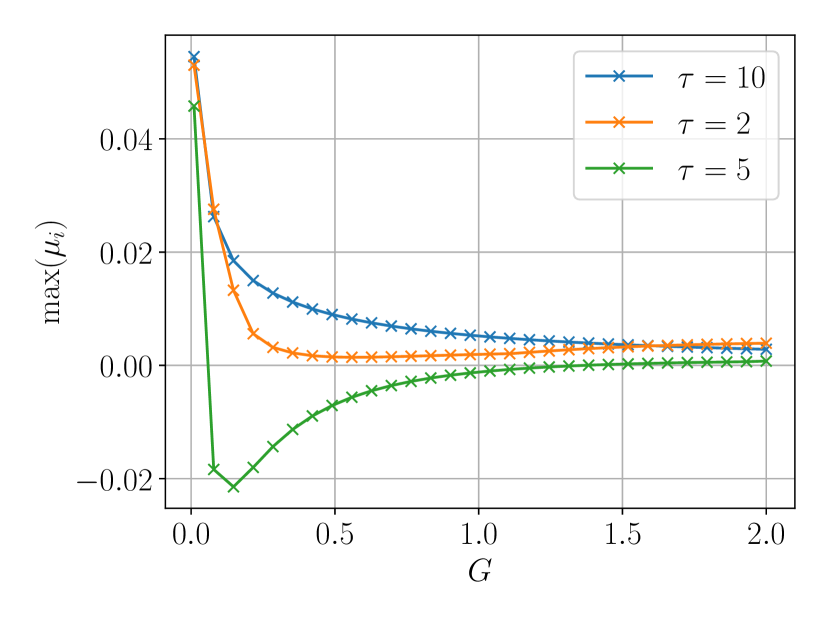
(b)

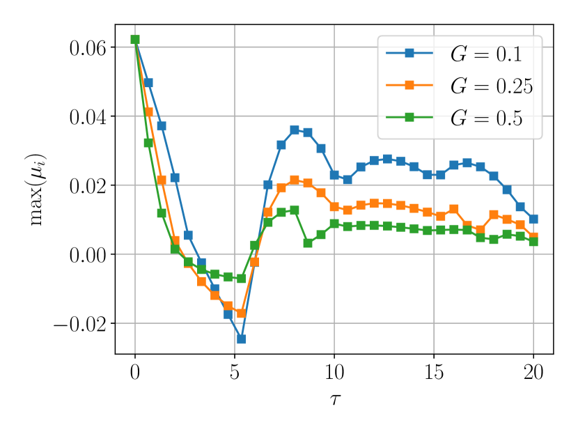
Figure 4: Dependence of the largest real-part of the eigenvalue spectrum $\max_{i}\mu_{i}$ ($\lambda_{i}=\mu_{i}+\mathrm{i}\omega_{i},$) with $G$ (left (a)) and $\tau,$ (right (b)) for $Re=2500$ UB solution, according to the approximate linear theory.

We can verify these predictions by performing some additional numerical simulations with TDF in the full Navier-Stokes equations. Figure 3 (b) demonstrates that stability is observed for $\tau=5$ and $G^{\mathrm{max}}=0.1.$ Moreover $G^{\mathrm{max}}=0.5$ is less strongly stable, and $\tau=2$, $G^{\mathrm{max}}=0.1$ is more strongly unstable, all of which is consistent with the above analysis. While this stability analysis is useful in validating and optimising TDF, it does not offer much insight into, for instance, why $\tau\approx 5$ is optimal in this example. Following the “frequency damping” interpretation of TDF (e.g. Akervik et al., 2006; Shaabani-Ardali et al., 2017), we define the transfer function

$$H_{\mathrm{TDF}}(\mathrm{i}\omega,\tau)=\frac{1}{G}\frac{\mathcal{L}\{\mathbf{F}_{\mathrm{T}DF}\}}{\mathcal{L}\{\mathbf{u}\}}=e^{-\mathrm{i}\omega\tau}-1$$

with $\mathcal{L}\{.\}(\omega)=\int_{0}^{\infty}.\,e^{-\omega t}dt$ the Laplace transform. The Laplace transform of the control term is $\mathcal{L}\{\mathbf{F}_{\mathrm{TDF}}\}(\omega)=-G(1-e^{-\omega\tau})\mathcal{L}\{u\}.$ $H_{\mathrm{TDF}}(\mathrm{i}\omega)$ allows us to ascertain the relative influence of the control term upon the temporal frequencies of the system in general (unlike a specific linear stability analysis). Figure 5 plots the magnitude of the transfer function against a normalised angular frequency. The first observation is that any zero mode is undamped by TDF control; this is an alternative explanation of the odd-number limitation where a purely real-valued eigenvalue cannot be stabilised in isolation. The next observation is that any harmonic of the feedback frequency $\frac{2\pi}{\tau}$ is also unaffected by the control. The consequence of these facts mean that any unstable eigenvalue of the target ECS with a frequency that is either close to zero, or close to the feedback frequency (or harmonic thereof) will not be stabilised. For high $Re$ travelling waves this means that careful tuning of the delay period, $\tau,$ may be necessary as the likelihood of an unstable eigenfrequency falling near a zero of the transfer function will increase.

We may use this analysis to interrogate the behaviour of TDF across a range of delay periods for the UB solution at $Re=2500$ discussed above. Defining $H_{n}(\tau)=|H_{\mathrm{TDF}}(\mathrm{i}\omega_{n},\tau)|$ with $\omega_{n}$ the unstable eigenfrequencies of the uncontrolled solution as shown in figure 2 (b), namely at $Re=2500,$ $\omega_{1}=0.75,\,\omega_{2}=0.48,\,\omega_{3}=0.32,$ we plot the product $H_{1}H_{2}H_{3}$ in figure 5. This demonstrates clear agreement with the linear analysis of figure 4 and therefore also the stabilisation of UB in figure 3. We see that the product of transfer functions is maximised at $\tau\approx 5$ and distinct zeros at harmonics of the eigenperiods, also coinciding with maxima of $\max(\mu)$ in figure 4. More specifically the first zero of $H_{1}H_{2}H_{3}$ is at $\tau=\frac{2\pi}{\omega_{1}}=8.25$ in the same location as the first maximum of $\max(\mu)$ for these parameters, indicating, as expected, TDF will fail for poorly chosen time delays.

3.4 A data-driven approach to setting TDF parameters

We have gained good insight into the behaviour of TDF in this example, however this analysis relies on knowledge of the unstable spectrum of the target solution. One goal when developing TDF would be the ability to obtain new, unknown solutions, without any knowledge of their properties in advance. In the example above we set off with this approach, i.e. $\tau=2$ and $G^{\max}=0.5,$ used in figure 3, are set speculatively after a little trial and error. If we examine the bifurcation which occurs at $Re\approx 2450$ with this TDF term active, we observe two complex conjugate pairs of eigenvalues crossing the axis with $\omega\approx 0.16\approx\omega_{2}/2$ and $\omega\approx 0.246\approx\omega_{2}/2.$ In fact when $|\lambda\tau|\ll 1,$ i.e. substituting $e^{-\lambda\tau}\approx 1-\lambda\tau$ in equation (25), we see that the effect of TDF on eigenvalues of $\mathcal{L}$ is rescaling by $1+G\tau.$ Hence, since $\tau$ is too small to effectively damp the lowest frequency eigenvalues, we observe them crossing the axis with frequencies $\frac{\omega}{1+G\tau}.$ This means, if we can capture an estimate of these frequencies it would be possible to perform the frequency domain analysis above and choose more carefully tailored $\tau.$ We might expect, near the onset of such supercritical bifurcations, to observe these frequencies in the numerical simulation. Taking the time-series for the total kinetic energy $E(t)$ for the $Re=2500$ case with $\tau=2$ and $G^{\max}=0.5,$ as shown in figure 3, and performing a Fourier transform, we observe, in figure 5 (b) a low-frequency/zero mode associated with a transient growth/decay of energy, but also two dominant modes almost exactly at $0.246$ and $0.16.$ Similarly we show the case with $\tau=2$ and $G^{\max}=0.1,$ which has peaks in the power spectrum at $\omega_{2}/1.2\approx 0.4$ and $\omega_{3}/1.2\approx 0.266,$ as we have predicted, but also $\omega_{2}/1.2-\omega_{3}/1.2,$ indicating some nonlinear interactions taking place at slightly larger amplitude from the bifurcation.

This approach may allow one, in theory, to diagnose more effective time-delays when TDF fails to stabilise a solution and results in an, invasive, low dimensional state.

(a)

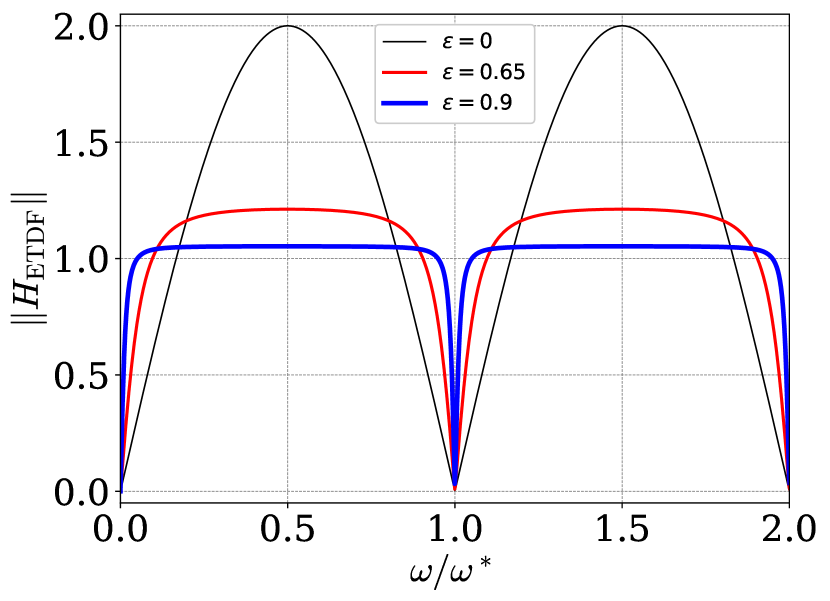
(b)

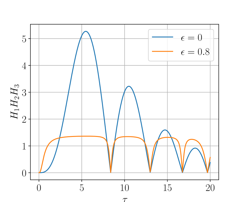
Figure 5: Transfer functions for TDF ($\epsilon=0$) and ETDF (various $\epsilon\neq 0$). (a) shows $H_{\mathrm{ETDF}}(\omega/\omega^{*})$ where $\omega^{*}=2\pi/\tau$ demonstrating peaks at subharmonics and zeros at harmonics of $\tau.$ (b) shows the product of $H_{n}=H_{\mathrm{ETDF}}(\omega_{n},\tau)$ for the three unstable eigenfrequencies of UB at $Re=2500.$ This indicates an optimal $\tau,$ for TDF, of around 5.5. This is consistent with the linear analysis shown in figure 4.

4 Generalising time-delayed feedback control

4.1 Extended time-delayed feedback

In the analysis of the previous section we observe relatively narrow operating windows for which TDF will stabilise the target solution, which, as expected, decrease as $Re$ in increases. A common way to address this problem is via “extended time-delayed feedback control” (ETDF). This feeds an extended historical record into the control term by including times $t-k\tau$ for increasing integers $k$ as time evolves. For our implementation this would read, neglecting, for now, translations in $z,$

$$F_{\mathrm{ETDF}}(t) = G\bigg{[}(1-\epsilon)\sum_{k=1}^{\infty}\epsilon^{k-1}u(t-k\tau)-u(t)\bigg{]}\>,$$ (26)

$$= G[u(t-\tau)-u(t)]+\epsilon F_{\mathrm{ETDF}}(t-\tau)\>,$$

where $0\leq\epsilon\leq 1$, see Socolar et al. (1994). $\epsilon=0$ reduces the control back to the standard Pyragas control. This has the effect of broadening and flattening the transfer function:

$$H_{\mathrm{ETDF}}(\mathrm{i}\omega,\tau)=\frac{1}{G}\frac{\mathcal{L}\{\mathbf{F}_{\mathrm{T}DF}\}}{\mathcal{L}\{\mathbf{u}\}}=\frac{e^{-\mathrm{i}\omega\tau}-1}{1-\epsilon e^{-\mathrm{i}\omega\tau}},$$

see figure 5. This method is attractive as it is relatively simple to implement and in practice only requires storing one additional history array for $F_{\mathrm{ETDF}}(t-\tau)$ (over a period). However, for our case, in particular for the analysis performed above with UB, we observe that the flattening of the transfer function results in much less distinct maxima, in particular the peak at $\tau=5.5$ is much smaller (Figure 5) and is unlikely to result in the same stabilisation observed with regular TDF. Moreover we have seen that attempting to stabilise states with several unstable eigenfrequencies is challenging, and ETDF gives only a marginal advantage in this regard, particularly if the frequencies are well separated.

4.2 Multiple time-delayed feedback

In the previous example for UB the instability observed at $Re=2500$ using $\tau=2$ was remedied following a careful analysis of the effect of TDF terms on the unstable eigenvalues of the uncontrolled system. It was noted that the frequencies are key in choosing an appropriate time-delay and that they may be observed in unsuccessful, invasive TDF dynamics.

To attenuate oscillations across several frequencies, we introduce multiple time-delayed feedback (MTDF), $\bm{F}_{\mathrm{MTDF}}$, such that

$$\bm{F}_{\mathrm{MTDF}}(r,\theta,z,t)=\sum_{i}^{N}G_{i}(t)[\mathcal{T}_{z}(s_{z})\bm{u}(r,\theta,z,t-\tau_{i})-\bm{u}(r,\theta,z,t)]\>,$$ (27)

where the $i$th time delay is $\tau_{i}$ ($i=1,2,\cdots,N$) and we translate the $i$-th delayed state, $\bm{u}(\bm{x},t-\tau_{i})$, by the streamwise shift, $s_{z}(t;\tau_{i})$. Delayed feedback with multiple delays was previously used in the low-dimensional chaotic system of Chua’s circuit by Ahlborn & Parlitz (2004), to stabilise a nonlinear steady solution. They reported that multiple time-delayed feedback helped to expand the basin of attraction of equilibrium solutions, being more efficient than extended time-delayed feedback (ETDF) (Socolar et al., 1994; Sukow et al., 1997).

We can repeat the analysis of § 3.3 with MTDF by simply introducing a second TDF term into equation (25). We will begin by investigating the effect of introducing a second term to the unstable $Re=2500$ case, i.e. $\tau_{1}=2,$ $G_{1}=0.5$ and varying $\tau_{2}$ and $G_{2}.$ Given that we have observed $\omega_{2}/2$ and $\omega_{3}/2$ in the TDF example, it would be sensible to choose a $\tau_{2}$ to stabilise these modes. Via the transfer function analysis of the previous section, now with $H_{n}^{*}=|H_{\mathrm{TDF}}(\mathrm{i}\omega_{n}/(1+G_{1}\tau_{1}),\tau_{2})|,$ we are again able to predict an optimal $\tau_{2}$. The maxima of the product $H_{2}^{*}H_{3}^{*}$ line up with the minima of $\max(\mu_{i})$ from the MTDF linear theory, indicating an optimal $\tau_{2}\approx 16$, see figures 6b and 7a. The interpretation here is that the second term should act to attenuate the frequencies modified by the first term (or vice-versa). It should also be noted that there is now a far larger range of $\tau_{2}$ and $G_{2}$ which stabilises UB, meaning less speculative tuning of parameters, particularly of $G_{2}.$

Note one could define a transfer function $H_{\mathrm{MTDF}},$ for MTDF, given by

$$H_{\mathrm{MTDF}}(\mathrm{i}\omega)=\frac{1}{\sum_{i}^{N}G_{i}}\frac{\mathcal{L}\{F_{\mathrm{MTDF}}\}}{\mathcal{L}\{u\}}=\frac{\sum_{i}^{N}G_{i}\exp(-i\omega\tau_{i})}{\sum_{i}^{N}G_{i}}-1$$ (28)

However applying this to the case under discussion effectively yields a repeat of the single TDF result, in that the optimal $\tau_{2}$ to stabilise the three eigenfrequencies, with $\tau_{1}=5,$ is around 5; $H_{\mathrm{MTDF}}$ does not accurately predict the effect of combinations of time-delays upon a given state.

(a)

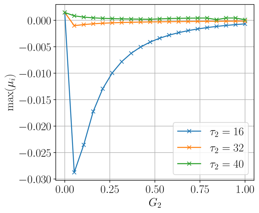
(b)

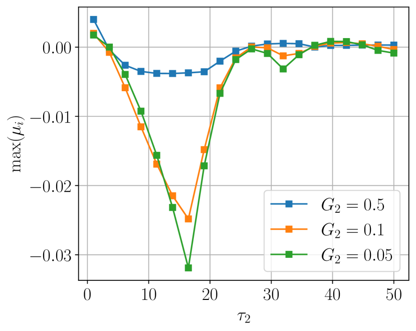
Figure 6: Dependence of the largest real-part of the eigenvalue spectrum $\max_{i}\mu_{i}$ with $G_{2}$ and $\tau_{2},$ for $Re=2500$ UB solution with two-term MTDF and $\tau_{1}=2$ and $G_{1}=0.5$. Most effective stabilisation is observed with $\tau_{2}\approx 16$ and the rather modest $G_{2}\approx 0.05.$

(a)

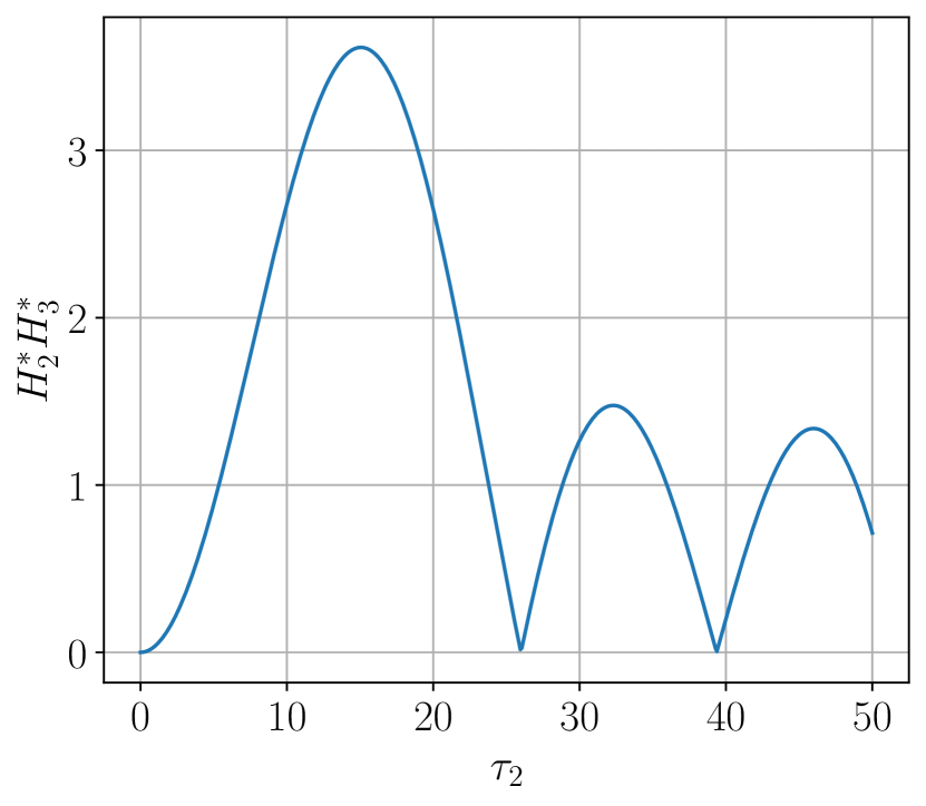
(b)

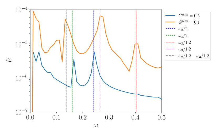
Figure 7: (a) shows the product of transfer functions $H_{1}^{*}H_{2}^{*}$ as defined in the text, for the modified eigenfrequencies when attempting to stabilise UB at $Re=2500$ using $\tau=2$ and $G=0.5.$ Note that the peak coincides with figure 6b, i.e. $\tau_{2}\approx 16$ is around the optimal. (b) shows the power spectrum of energy, $\hat{E}$, for the unsuccessful TDF cases at $Re=2500$ with $\tau=2$ and $G=0.5$ and 0.1. Vertical lines show that the peaks in these spectra follow the expected scaling by $1/(1+\tau G).$

(a)

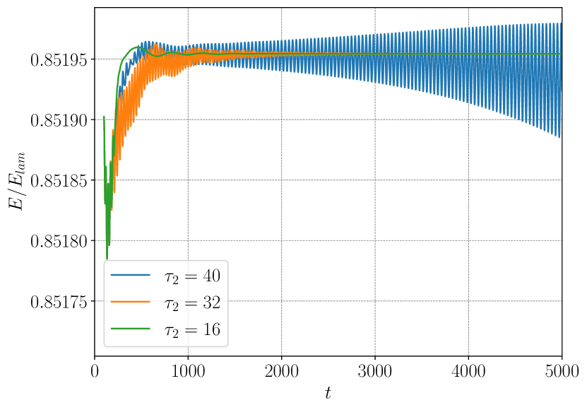
(b)

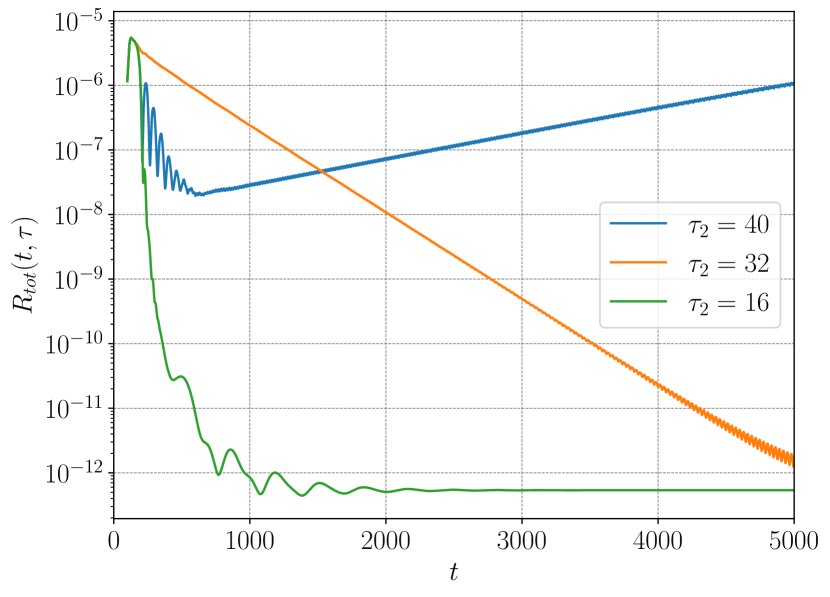
Figure 8: MTDF stabilisation of UB travelling wave at $Re=2500$, shown via time series of $E/E_{\mathrm{lam}}$ (a) and $R_{\mathrm{tot}}$ (b). Comparison shows various choices of $\tau_{2}$ with $\tau_{1}=2,$ $G_{1}=0.5,$ and $G_{2}=0.1.$ We see rapid stabilisation for the optimal $\tau_{2}=16,$ moderate stabilisation for $\tau_{2}=32$ and instability for $\tau=40.$

5 Stabilisation of nonlinear travelling wave from turbulence

Having described the ability of MTDF to successfully damp instability of nonlinear travelling waves, in this section we will demonstrate that such stabilised states can have suitably large basins of attractions and that it is possible to stabilise them from turbulence. We proceed as if the properties of the target solutions are unknown and allow the multiscale fluctuations of turbulence to fully develop before attempting stabilisation using MTDF. Turbulent fluctuations may include much longer timescales than the eigenperiods of the target solution. We imagine that some well chosen delays can suppress sufficient spatiotemporal fluctuations in turbulence, without relaminarising the flow completely, at the same time as achieving stabilisation of the target solution. In other words, there is some motivation for including MTDF terms to widen the basin of attraction of the target state, as well as to force eigenvalues across the imaginary axis. However, this introduces a challenge: the more delays we use, the more parameters we need to adjust to stabilise nonlinear travelling waves successfully.

Without prior knowledge of the solution’s instability, we seek to exploit some automatic techniques for obtaining stabilising parameter values. We have seen how $\tau_{i}$ may be chosen in some data-driven manner; in the next section we discuss the adaptive gain method of (Lehnert et al., 2011), which automates the selection of $G$ and seeks to avoid a laborious parameter search.

(a)

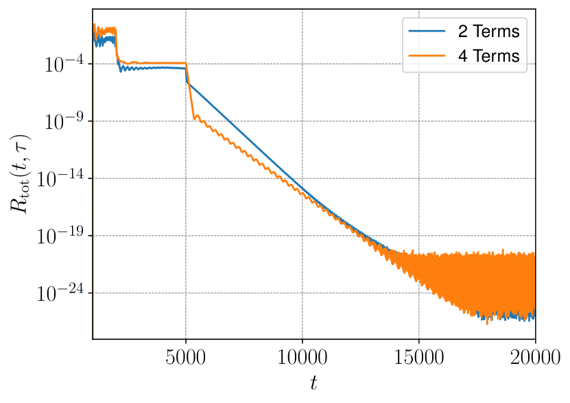
(b)

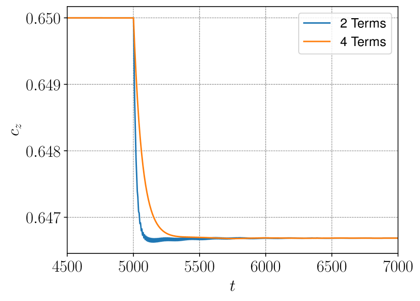
(c)

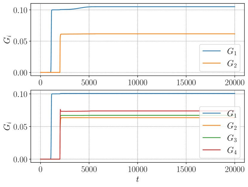
(d)

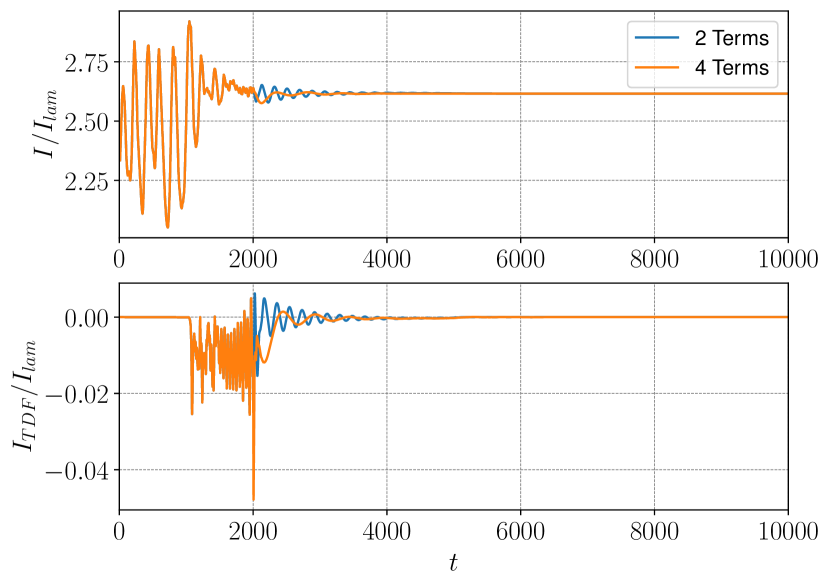
Figure 9: Successful stabilisation of UB at $Re=3000$ from a turbulent state using MTDF (27) with two terms ($\tau_{1}=2$, $\tau_{2}=9$) and four terms ($\tau_{1}=2$, $\tau_{2}=9$, $\tau_{3}=17,$ $\tau_{4}=33$). (a) $R_{\mathrm{tot}}$, (b) $c_{z}$. (c) $G_{i}$, The gain, $G_{1}(t)$, is switched on at $t=1000$. Here, $G_{1}(t)$ is initially increased following the sigmoid gain function (19) where ($t_{s}$,$G_{1}^{\max}$,$a$,$b$)=(1000,0.1,0.1,100). Then at $t=2000$ $G_{i}$ evolves via the adaptive method equation (35) where $\gamma_{i}^{G}=0.1$ for all terms. The adaptive shift method is switched on at $t=5000$, where $\gamma^{s}=0.1$ and $c_{z}(0)=0.65$.

(a)

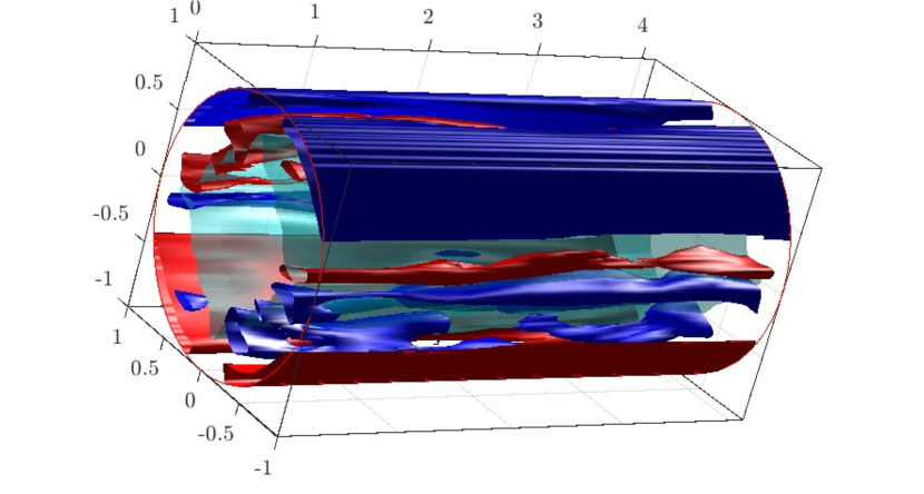
(b)

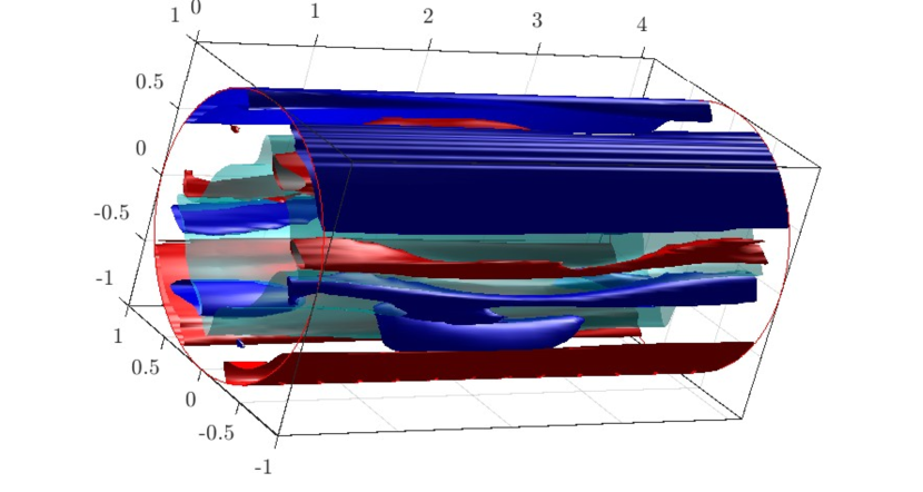
Figure 10: Two snapshots from the simulation using MTDF with two delays (see figure 9). (a) Turbulent field at $t=10000$ and (b) stabilised UB at $t=30000$. The cyan isosurface denotes $u_{z}=-0.1$. The red and blue isosurfaces denote $\omega_{z}=0.15$ and $-0.15$, respectively, where $\omega_{z}=(\nabla\times\bm{u})_{z}$ is the streamwise fluctuating vorticity.

5.1 Adaptive gain method

The speed-gradient method of Lehnert et al. (2011) seeks to find an optimal TDF gain by dynamically adjusting $G(t)$ by a gradient descent method. In order to exploit this method, we need to extend it to handle multiple terms and the translation operator which is applied to the control term(s). We define the cost function, $Q_{i}(t)$, for the $i$-th feedback term as:

$$Q_{i}(t)=\frac{1}{2}\int|\mathcal{T}_{z}(s_{z})\bm{u}(\bm{x},t-\tau_{i})-\bm{u}(\bm{x},t)|^{2}\mathrm{d}V\>,$$ (29)

and successful control yields $Q_{i}(t)\rightarrow 0$ as $t\rightarrow\infty$. The speed gradient algorithm in the differential form is given by

$$\frac{\mathrm{d}}{\mathrm{d}t}{G}_{i}(t)=-\gamma_{i}^{G}\nabla_{G_{i}}\frac{\mathrm{d}{Q}_{i}}{\mathrm{d}t}\>,$$ (30)

where $\gamma_{i}^{G}>0$ is a free parameter controlling the descent rate and $\nabla_{G_{i}}$ denotes $\partial/\partial G_{i}$. By taking time-derivative of (29), we have

$$\frac{\mathrm{d}{Q}_{i}}{\mathrm{d}t}=\int g_{i}(\bm{x},t)\mathrm{d}V\>,$$ (31)

where

$$g_{i}(\bm{x},t)=[\mathcal{T}_{z}(s_{z})\bm{u}(\bm{x},t-\tau_{i})-\bm{u}(\bm{x},t)]\bigg{[}\mathcal{T}_{z}(s_{z})\frac{\partial\bm{u}}{\partial t}(\bm{x},t-\tau_{i})-\frac{\partial\bm{u}}{\partial t}(\bm{x},t)\bigg{]}$$ (32)

and we have assumed that $\gamma_{s}$ is chosen such that $\frac{\mathrm{d}s_{z}}{\mathrm{d}t}\ll 1,$ hence $s_{z}$ is approximately constant for the purposes of updating $G_{i}(t).$ Using the Navier–Stokes momentum equations with MTDF in the form

$$\frac{\partial}{\partial t}\bm{u}(\bm{x},t)=\bm{f}(\bm{x},t)+\sum_{i}^{N}G_{i}[\mathcal{T}_{z}(s_{z})\bm{u}(\bm{x},t-\tau_{i})-\bm{u}(\bm{x},t)]\>,$$ (33)

where $\bm{f}$ includes all the terms from the right-hand side of the momentum equation, alongside (30) and (31), we obtain the following formula:

$$\frac{\mathrm{d}}{\mathrm{d}t}{G}_{i}(t)=-\gamma_{i}^{G}\int h_{i}(\bm{x},t)\mathrm{d}V,$$ (34)

where

$$h_{i}(\bm{x},t)=[\mathcal{T}_{z}(s_{z})\bm{u}(\bm{x},t-\tau_{i})-\bm{u}(\bm{x},t)]\\ [\bm{u}(\bm{x},t)-2\mathcal{T}_{z}(s_{z})\bm{u}(\bm{x},t-\tau_{i})+\mathcal{T}_{z}(2s_{z})\bm{u}(\bm{x},t-2\tau_{i})]\>.$$ (35)

Note than on taking $\nabla_{G_{i}}$ only the MTDF terms contribute to $h_{i}.$ Equation (35) indicates that the code should store instantaneous velocity field data over 2 delay periods, $2\tau_{i},$ when using this adaptive gain method, hence doubling the storage requirements, However, we implement a temporal interpolation procedure using cubic splines (Shaabani-Ardali et al., 2017) to enable us to store longer historical records of $\bm{u}$ albeit at the cost of some approximation error in the interpolation method.

5.2 Results

Here we attempt to stabilise UB at $Re=3000$ from a turbulent state, in the ($S$,$Z_{2}$)-symmetric invariant subspace using MTDF. In this subspace, UB at $Re=3000$ has 4 pairs of complex unstable eigenvalues, and therefore it is unaffected by the odd-number limitation (Nakajima, 1997). We approach this problem as if the eigenvalues are unknown and we select $\tau_{i}$’s and other MTDF parameters without any linear analysis to steer our choices.

We consider first an MTDF case with two delays, $(\tau_{1},\tau_{2})=(2,9)$. We set the following parameters for $\tau_{1}$; ($t_{s}$,$G^{\max}$,$a$,$b$,$\gamma^{s}$)=(1000,0.5,0.1,100,0.1), i.e. TDF becomes active at $t=1000,$ giving a period of turbulent activity, and an an initial sigmoid profile of $G(t)$. The adaptive gain method for $G_{1}(t)$, with $\gamma_{1}^{G}=0.1$, is then started at $t=2000$, and $G_{1}(t)$ evolves following the ODE (30). The second feedback term with gain, $G_{2}(t)$, evolves from zero at $t=2000$ through the adaptive gain method ($\gamma_{2}^{G}=0.1$). Without knowing successful values of $G_{i}$ and $s_{z}(t;\tau_{i})$ in advance, we successfully stabilise UB at $Re=3000$ using this double-delay MTDF (see figure 9). In order to verify the non-invasive nature of the stabilisation in the MTDF cases, the definition of $R_{\mathrm{tot}}$ requires updating

$$R_{\mathrm{tot}}=\frac{\|\sum_{i}^{N}\left[\mathcal{T}_{z}(s_{z})\bm{U}(r,\theta,z,t-\tau_{i})-\bm{U}(r,\theta,z,t)\right]\|_{2}}{\|\bm{U}(r,\theta,z,t)\|_{2}}.$$ (36)

Successful, non-invasive stabilisation is quantitatively confirmed by the very small values of both $R_{\mathrm{tot}}$ (figure 9 (a)) and $I_{\mathrm{TDF}}/I_{\mathrm{lam}}$, the latter being of order of $10^{-8}$ at $t=10000$ (see figure 9 (d)). $c_{z}$ is also evolved onto it’s exact value through the adaptive translation method and we observe $G_{i}$ being adjusted by the speed-gradient method onto stabilising values. A snapshot of the stabilised UB at $t=10000$ is shown in figure 10(b) with a turbulent field at $t=1000$ for comparison in figure 10(a).

Figure 9 also shows an MTDF case with four delays where $\tau_{1}=2$, $\tau_{2}=9$, $\tau_{3}=17$, $\tau_{4}=33$. Motivated by our frequency-domain analysis in § 3.3, these delays are carefully chosen to be non-commensurate and provide broad coverage of the temporal spectrum. As in the two-delay case, only $G_{1}(t)$ is switched on at $t=1000$ following the sigmoid gain funtion (19) , where ($t_{s}$,$G_{1}^{\max}$,$a$,$b$,$\gamma^{s}$)=(1000,0.1,0.1,100,0.1). The adaptive gain method is switched on at $t=2000$ with $\gamma^{G}=0.1$ for all the terms, . Once the time-dependent gains are turned on, $I_{\mathrm{TDF}}/I_{\mathrm{lam}}$ starts to fluctuate with the amplitude smaller than 0.02 and then exhibits a damped oscillatory behaviour, similar to the case with two delays. There are no significant qualitative differences between the two and four term MTDF cases; in the four delay case $G_{3}$ is the second largest (recall $\tau_{3}=17$) and $G_{2}$ takes a smaller value at stabilisation than the two-delay case. $G_{4}$ is the smallest but still make a significant contribution. This suggests that the terms are all influencing the stabilisation, while the two-delay case demonstrates that not all terms are necessary for stabilisation. The rate of attraction is of the same order in both cases, this may suggest that the principle benefit of additional terms in MTDF is to widen the parameter windows under which UB is stabilised. If stabilising $G$ are not obtained, it may be observed that the state is brought near the target solution, but then moves away from it along some unstable manifold, similar to the blue curves in figure 8. The adaptive method gives the gains freedom to find values which succeed in stabilisation, instead of this close approach. It is worth noting that the energy injected by the forcing is only around 2-3% of the energy injected by the imposed pressure gradient, see figure 9(d). This means that, even at early times when the MTDF terms are largest, the overall energetic influence of MTDF on the flow is quite small. This may provide motivation for development of TDF or MTDF in real-world experimental control situations; TDF does not need to intervene strongly to stabilise these travelling waves.

(a)

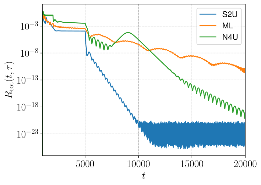
(b)

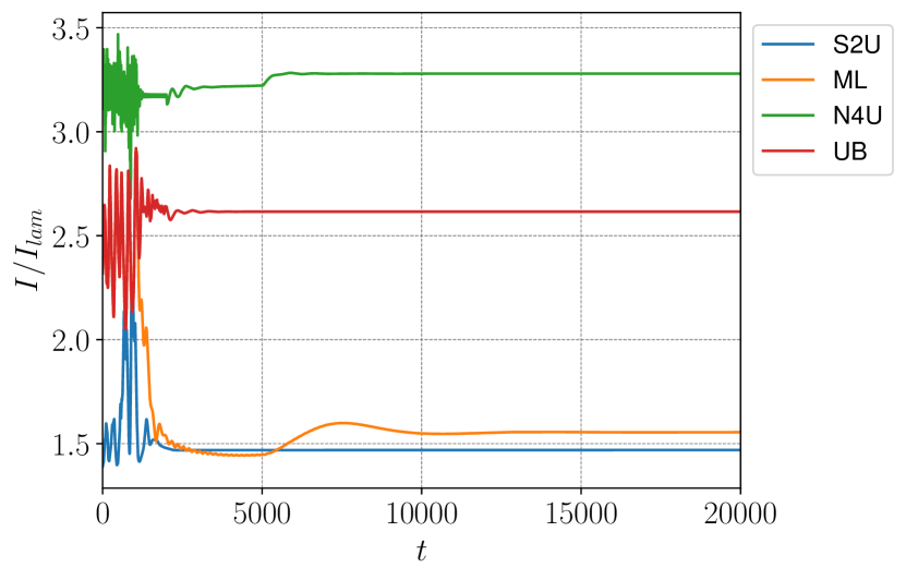
(c)

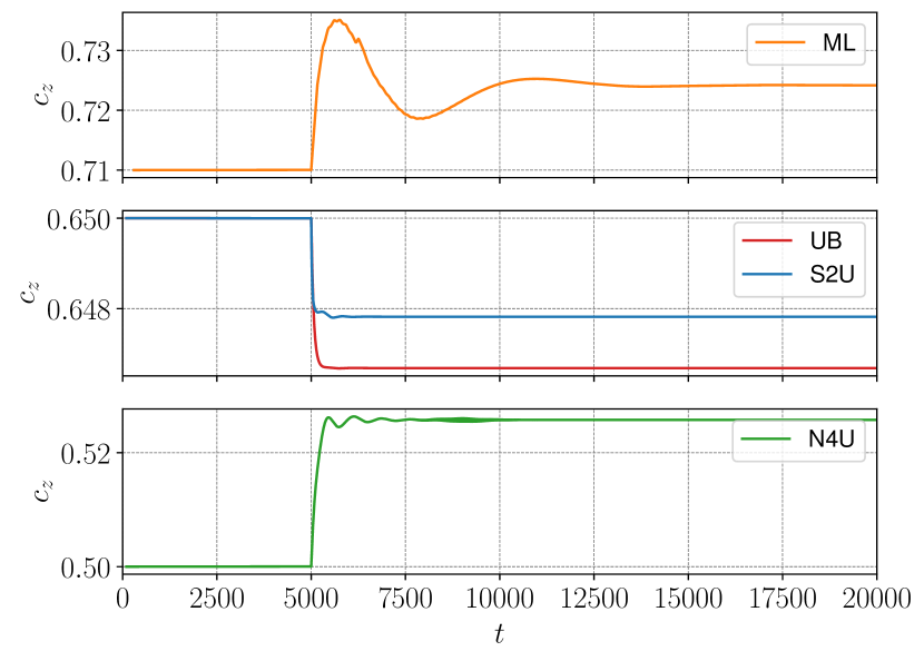
(d)

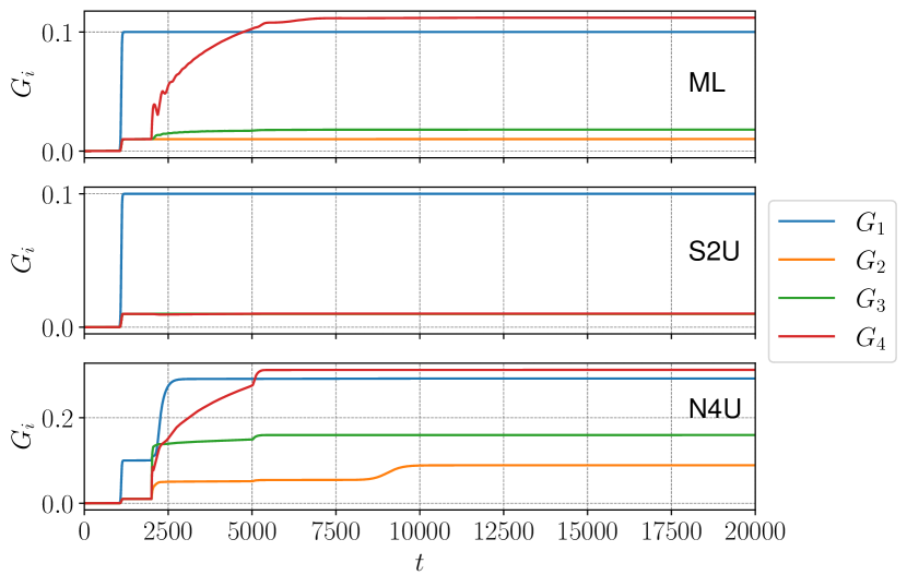
Figure 11: Plots showing successful stabilisation of S2U, ML, N4U in their respective subspaces, from a turbulent state using four-term MTDF (27). Specific parameter values can be found in table 2. (a) Shows the residual $R_{\mathrm{tot}},$ (b) the energy input $I/I_{\mathrm{lam}},$ (c) the phase speeds $c_{z}$ dynamically converging to their exact values, and (d) the time-dependent gains $G_{i}(t).$

(a)

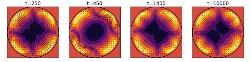
(b)

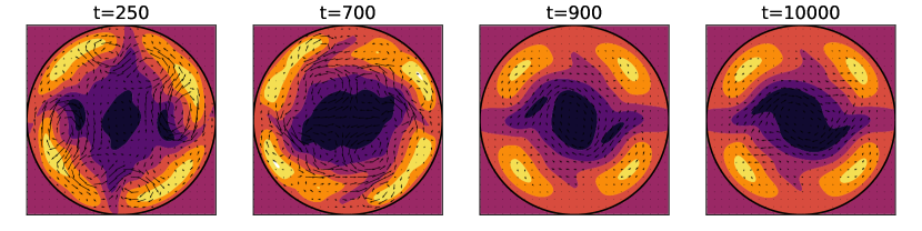
(c)

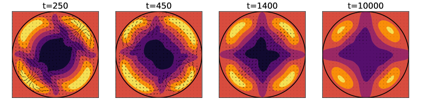
(d)

Figure 12: Snapshots of the $(r,\theta)$ plane at $z=0$ in the frame of reference translating with $c_{z}$ of the travelling waves for the MTDF cases outlined in table 2 From top to bottom (a) UB (b) S2U (c) ML N4U. Coloured contours represent $u_{z}$ (each with 7 contours evenly spaced in $[-0.45,0.45]$ except S2U which uses $[-0.35,0.35]$) and arrows to represent the in-plane velocity vector. Final snapshot at $t=1000$ shows the stabilised state.

5.3 Travelling waves S2U, ML, N3 and N4U

Having shown that UB is able to be stabilised from the turbulent state by our adaptive MTDF approach, we now demonstrate the generality of these results by presenting the stabilisation of the other travelling waves outlined in table 1, the stabilising parameters can be found in table 2.

sol.	sym.	$Re$	$\alpha$	$\tau_{1}$	$\tau_{2}$	$\tau_{3}$	$\tau_{4}$	$G_{1}^{\max}$	$G_{i\neq 1}^{\max}$	$\gamma^{G}$	$c_{z}(0)$
UB	$S$,$Z_{2}$	$3000$	1.25	2	9	17	33	0.1	0	0.1	0.65
ML	$S$,$Z_{2}$	$3000$	1.25	2	9	33	150	0.1	0.01	0.5	0.71
S2U	$S$	$2400$	1.25	2	9	17	33	0.1	0.01	0.1	0.65
N4U	$S$,$Z_{4}$	$2500$	1.7	2	9	17	33	0.1	0.01	0.1	0.5

Table 2: Table summarising the parameters used in the four-term MTDF stabilisation of the travelling waves discussed. In all cases the start time $t_{s}=1000$ is used, $a=0.1,\,b=100$ for the sigmoid initialisation of $G_{i}$ with adaptivity started at $t=2000$ for all terms in all cases. Adaptivity of the translation (or phase speed) is initiated at $t=5000$ with $\gamma^{s}=0.1$ in all casses, with initial value shown in the table as $c_{z}(0)$.

First we tackle S2U at $Re=2400$ in the $S$ symmetry subspace where the solution has one pair of unstable eigenvalues $\lambda_{\pm}=0.14\pm 0.13\mathrm{i}$ (note in the full space this solution violates the odd-number condition, see table 1). In theory this solution should be able to be stabilised with a single TDF term, provided $\tau$ and $G$ take suitable values. However, as in the previous case, we continue with MTDF as though we did not know the stability information, and start from the turbulent attractor. We use four terms with the same choices for $\tau_{i},$ i.e. 2, 9, 17 and 33, as before. In the course of calibrating our adaptive methods it was noted that starting $G_{i}$ from 0 could lead to some slight instability; individual “speed-gradients” begin with a large value (not only when targeting this solution but in general). A simple way to avoid this is to begin with small non-zero gains before starting to adapt, but again initialised with a sigmoid function. In this case we keep all other parameters the same as the four term UB case of figure 9, only with $G_{i}^{\max}=0.01$ for $i=2,3,4,$ and in the $S$ subspace, see table 2. Figure 11 shows a similar picture to figure 9, this time the gains do not undergo any significant dynamical adjustment and S2U is rapidly stabilised. An accurate $c_{z}$ is again able to be obtained and the residual is observed becoming very small. Figure 12(b) shows snapshots of this stabilisation.

ML is quite weakly unstable, in the $(S,Z_{2})$ subspace at $Re=3000$ and the solution has only one unstable direction with $\lambda_{\pm}=0.0087\pm 0.019\mathrm{i}.$ This provides a useful test case to demonstrate that in this subspace at this Reynolds number, multiple solutions can be stabilised by only adjusting the MTDF parameters without requiring special treatment of the initial condition. Note that the unstable eigenfrequency is very small for this solution which necessitates using larger delay periods, tests with similar parameters used to stabilise UB either restabilise UB or relaminarise. In this instance we choose $\tau_{i}\in{2,9,33,150}$ and initiate with $c_{z}(0)=0.71,$ the only other difference from earlier cases is that $\gamma^{G}=0.5$ for all terms (see table 2). As is shown in figure 11, ML, despite being much less unstable that the other cases we have studied, shows weaker stabilisation. In addition we see that $G_{4}$ undergoes significant growth once the speed-gradient method is initiated at $t=2000,$ becoming the largest gain of the four. Only once $G_{4}$ has grown do we observe the solution stabilising, indicating that this term is dominant in ensuring stabilisation, which is consistent with the frequency domain analysis. In retrospect a larger starting $G^{\max}_{4}$ is likely to improve the stabilisation of ML. Nevertheless the adaptive approach has been able to determine stabilising gains automatically. Figure 12(c) shows snapshots of this stabilisation.

Noting that ML and UB have been successfully stabilised at the same Reynolds number, in the same symmetry subspace and with quite similar MTDF parameters, we have verified that taking the parameters used to stabilise ML (row 2 of table 2) and changing only $c_{z}(0)=0.65$ results in the stabilisation of UB. In other words both solutions can be obtained varying only $c_{z}(0).$

N4U is stabilised in the $(S,Z_{4})$ subspace, $Re=2500,\,\alpha=1.7$ with the same MTDF parameters used in the S2U case only now with $c_{z}(0)=0.5,$ as outlined in table 2. There are few significant differences in this case, $G_{4}$ and $G_{1}$ both grow to values $\approx 0.3$ with $G_{3}$ also becoming relatively large. As with earlier examples an analysis of the unstable eigenfrequencies would indicate which terms are necessary in this case, but in the interests of brevity we will not repeat a similar calculation here, noting that, even without this analysis, significant parameter tuning was not necessary to stabilise this solution. As with the other travelling waves, the residual $R_{\mathrm{tot}}$ only begins to fall to values for which MTDF may be considered non-invasive as the phase-speed converges to its final value, i.e. $t>5000$. Figure 12(d) shows snapshots of this stabilisation.

N3 presents another interesting case. In $S,Z_{3}$ the solution is stable, meaning that stabilisation is not necessary. However we have confirmed that by applying the symmetry operator $SZ_{3}$ to the TDF terms, e.g.

$$\bm{F}_{\mathrm{MTDF}}(r,\theta,z,t)=\sum_{i}^{N}G_{i}(t)[SZ_{3}\mathcal{T}_{z}(s_{z})\bm{u}(r,\theta,z,t-\tau_{i})-\bm{u}(r,\theta,z,t)]\>,$$ (37)

stabilisation can be obtained in the full-space with some arbitrary (small) $\tau$ and $G.$ As explained in Lucas & Yasuda (2022), TDF or MTDF will simply drive the dynamics onto the symmetry subspace where the travelling wave is an attractor. This result suggests that the MTDF results shown earlier could be repeated in less-restrictive subspaces, with symmetry operators embedded in the MTDF terms, similarly to Lucas & Yasuda (2022).

6 Conclusion

In this paper, we present the first successful non-invasive stabilisation of nonlinear travelling waves in a straight circular pipe through the use of an improved control method involving time-delayed feedback (TDF). Our novel TDF protocol allows for the stabilisation of multiple nonlinear travelling waves, at a range of Reynolds numbers, in a variety of symmetry subspaces, from a generic turbulent history and with speculative control parameters.

Furthermore, our development of the TDF method has led to a deeper understanding of the principles governing time-delayed feedback in terms of an “approximate” linear stability analysis and frequency-domain analysis (see e.g., § 3.2). We have shown that the effect of TDF and MTDF on the unstable part of solution’s eigenvalue spectrum can be approximated surprisingly well, enough to point a parameter study in the right direction. Moreover it has provided clearer insight into the frequency domain interpretation of the control method, which in turn gives a helpful means to choose delay periods in these cases. Finally we have shown that, if stabilisation is nearly achieved, it can be possible to diagnose eigenfrequencies and hence pick more appropriate time-delays, using a data-driven approach, without the need for an a’priori stability analysis of the target solution. How practical this approach would be in an attempt to stabilise a real unknown solution remains to be seen, however this is a promising first step.

In order to enhance the performance of our TDF method, we implemented several optimisation methods that enables the feedback term(s) to vanish, as depicted in figure 9b. Because the bulk flow in pipe flow is driven by an imposed axial pressure gradient, all invariant solutions take the form of relative solutions, such as travelling waves and relative periodic orbits. Therefore, applying a translation operator to the delay term(s) is essential. To achieve this, we utilised the adaptive shift method (see § 3), which dynamically adjusts the translations to match the phase speeds of the target solution through a simple ODE (20). We have demonstrated here, for the first time, that by changing the initial condition for $s_{z},$ or $c_{z}$ different travelling waves can be stabilised.

In the chaotic pipe flow system, we find that multiple time-delayed feedback control (MTDF) is effective at improving the control’s ability to stabilise a wide range of unstable eigenfrequencies, as shown in § 4.2. A helpful consequence of MTDF is that it will serve to damp very slow temporal oscillations, which are typical in pipe flow (Shih et al., 2016). As demonstrated in the results of § 5.2 and § 5.3 successful stabilisations are found when MTDF is initiated with a short time delay ($\tau_{1}=2$ in all our cases), which acts for some time period before the rest of the terms become active. The effect is to suppress slow oscillations, importantly without relaminarising, giving the remaining terms a better chance at controlling the target travelling wave. In other words this initial delay is an effective means to widen the basin of attraction. In some cases $\tau_{1}$ contributes directly to altering the linear stability of the travelling waves, in others it only provides a nonlinear effect.

We have also sought to avoid expensive parametric studies. To achieve this, we have introduced the adaptive gain method (§ 5.1) into our TDF protocol. This method automates our search for an appropriate gain, thereby avoiding an exhaustive parametric search for $G_{i}$. We have observed this approach to be highly effective, for instance in § 5.3 when stabilising ML the longest time delay gain $G_{4}$ is observed to grow significantly, compared to the other terms, showing that $\tau=150$ was important in ensuring stabilisation. This is consistent with our frequency analysis when noticing that this travelling wave has a very large unstable eigenperiod of around 330.

During this work we have demonstrated that TDF, or more accurately MTDF, can stabilise multiple states at the same parameter values. In other words multiple attractors can coexist; UB and ML are stabilised varying only the initial $c_{z}.$ In this example the two states are relatively well separated in phase-space (upper and lower branch solutions, see figure 1) so it is perhaps surprising that ML is stabilised from a turbulent initial condition. This is a promising result as it demonstrates that the method does not require significant intervention to move from one solution to the next, however it does opens up a number of interesting questions. In particular, how might one design a systematic search, or data-driven approach, to explore basins of attraction of various potential stabilisable solutions? For instance UB at $Re=2400$ in the $S$ subspace is highly unstable and has 9 complex pairs of eigenvalues, in theory this could be stabilised by MTDF, however it will “compete” with S2U which is much less unstable (1 unstable direction), is also upper branch and has a very similar phase speed (see table 1). If any of the 9 eigenvalues has a particularly small eigenfrequency, necessitating a long time-delay, then close proximity to the solution is likely to be necessary for any stabilisation to be successful.

We have also seen that trialling various subspaces and/or embedding symmetry operators into TDF terms is a useful way to obtain different solutions, avoid the odd-number issue and avoid dealing with multiple attractors. However we have not conducted an exhaustive search of all possible subspaces, pipe lengths and $Re.$ We expect there will be many other travelling wave solutions, or even relative periodic orbits, which can be stabilised with TDF, not to mention in other wall-bounded shear flows.

In this paper, we have not tackled the odd-number limitation (Nakajima, 1997), which is a contentious issue in the TDF literature. Further improvements of this method are necessary in order to stabilise odd-number solutions. One possibility is the half-period TDF (Nakajima & Ueda, 1998a) which is similar in spirit to the use of symmetries here and in Lucas & Yasuda (2022). Another is “act-and-wait” TDF (Pyragas & Pyragas, 2018, 2019), where a time-dependent switching of the TDF gain is applied meaning uncontrolled dynamics are always used in the delay period, or “unstable ETDF” (Pyragas, 2001), where an additional unstable degree of freedom is introduced into the problem to create an even pair of exponents. We have demonstrated that there is some potential for this method in controlling nonlinear states in spatiotemporal chaos, which will hopefully serve as motivation for further developments tackling both the odd-number issue and even higher dimensional problems at large Reynolds number and in large domains. Potentially the most promising avenue for TDF in fluid flows is as a control method in a real physical system where a non-trivial flow state, perhaps of a specific dissipation or mixing rate, is desired but full spatiotemporal chaos is not. We have shown that with careful application of a time-delayed approach various kinds of target solution can be relatively easily obtained with minimal intervention.

[Funding]This work is supported by EPSRC New Investigator Award EP/S037055/1, “Stabilisation of exact coherent structures in fluid turbulence.”

References

- Ahlborn & Parlitz (2004) Ahlborn, A. & Parlitz, U. 2004 Stabilizing unstable steady states using multiple delay feedback control. Phys. Rev. Lett. 93, 264101.
- Akervik et al. (2006) Akervik, E., Brandt, L., Henningson, D. S., Hoepffner, J. & Schlatter, P. 2006 Steady solutions of the Navier–Stokes equations by selective frequency damping. Phys. Fluids 18, 068102.
- Azimi et al. (2020) Azimi, Sajjad, Ashtari, Omid & Schneider, Tobias M 2020 Adjoint-based variational method for constructing periodic orbits of high-dimensional chaotic systems. arXiv preprint arXiv:2007.06427 .
- Beaume et al. (2011) Beaume, Cédric, Bergeon, Alain & Knobloch, Edgar 2011 Homoclinic snaking of localized states in doubly diffusive convection. Physics of Fluids 23 (9), 094102.
- Budanur et al. (2017) Budanur, N. B., Short, K. Y., Farazmand, M., Willis, A. P. & Cvitanović, P. 2017 Relative periodic orbits form the backbone of turbulent pipe flow. J. Fluid Mech. 833, 274–301.
- Chandler & Kerswell (2013) Chandler, Gary J & Kerswell, Rich R 2013 Invariant recurrent solutions embedded in a turbulent two-dimensional Kolmogorov flow. Journal of Fluid Mechanics 722, 554–595.
- Darbyshire & Mullin (2006) Darbyshire, A. G. & Mullin, T. 2006 Transition to turbulence in constant-mass-flux pipe flow. J. Fluid Mech. 289, 83–114.
- Duguet et al. (2008a) Duguet, Y., Pringle, C. C. T. & Kerswell, R. R. 2008a Relative periodic orbits in transitional pipe flow. Phys. Fluids 20 (11), 114102.
- Duguet et al. (2008b) Duguet, Y., Willis, A. P. & Kerswell, R. R. 2008b Transition in pipe flow: the saddle structure on the boundary of turbulence. J. Fluid Mech. 613, 255–274.
- Faisst & Eckhardt (2003) Faisst, H. & Eckhardt, B. 2003 Traveling waves in pipe flow. Phys. Rev. Lett. 91, 224502.
- Farazmand (2016) Farazmand, M 2016 An adjoint-based approach for finding invariant solutions of Navier–Stokes equations. Journal of Fluid Mechanics 795, 278–312.
- Fiedler et al. (2011) Fiedler, B, Flunkert, V, Hövel, P & Schöll, E 2011 Beyond the odd number limitation of time-delayed feedback control of periodic orbits. The European Physical Journal Special Topics 191 (1), 53–70.
- Flunkert & Schöll (2011) Flunkert, V & Schöll, E 2011 Towards easier realization of time-delayed feedback control of odd-number orbits. Physical Review E 84 (1), 71–12.
- Graham & Floryan (2021) Graham, M. D. & Floryan, D. 2021 Exact coherent states and the nonlinear dynamics of wall-bounded turbulent flows. Annu. Rev. Fluid Mech. 53, 227–253.
- Hof et al. (2006) Hof, Björn, Westerweel, Jerry, Schneider, Tobias M & Eckhardt, Bruno 2006 Finite lifetime of turbulence in shear flows. Nature 443 (7107), 59–62.
- Itano & Toh (2001) Itano, Tomoaki & Toh, Sadayoshi 2001 The Dynamics of Bursting Process in Wall Turbulence. Journal of the Physical Society of Japan 70 (3), 703–716.
- Just et al. (1999) Just, Wolfram, Reibold, Ekkehard, Benner, Harmut, Kacperski, Krzysztof, Fronczak, Piotr & Hołyst, Janusz 1999 Limits of time-delayed feedback control. Physics Letters A 254 (3), 158 – 164.
- Kawahara et al. (2012) Kawahara, Genta, Uhlmann, Markus & van Veen, Lennaert 2012 The Significance of Simple Invariant Solutions in Turbulent Flows. Annual Review of Fluid Mechanics 44 (1), 203–225.
- Kreilos & Eckhardt (2012) Kreilos, Tobias & Eckhardt, Bruno 2012 Periodic orbits near onset of chaos in plane Couette flow. Chaos: An Interdisciplinary Journal of Nonlinear Science 22 (4), 047505.
- Lehnert et al. (2011) Lehnert, J, Hövel, P, Flunkert, V, Guzenko, P Yu, Fradkov, A L & Schöll, E 2011 Adaptive tuning of feedback gain in time-delayed feedback control. Chaos: An Interdisciplinary Journal of Nonlinear Science 21 (4), 043111–7.
- Lucas & Caulfield (2017) Lucas, Dan & Caulfield, C. P. 2017 Irreversible mixing by unstable periodic orbits in buoyancy dominated stratified turbulence. Journal of Fluid Mechanics 832.
- Lucas et al. (2017) Lucas, Dan, Caulfield, C. P. & Kerswell, Rich R. 2017 Layer formation in horizontally forced stratified turbulence: connecting exact coherent structures to linear instabilities. Journal of Fluid Mechanics 832, 409—437.
- Lucas & Kerswell (2017) Lucas, Dan & Kerswell, Rich 2017 Sustaining processes from recurrent flows in body-forced turbulence. Journal of Fluid Mechanics 817, R3–11.
- Lucas & Kerswell (2015) Lucas, Dan & Kerswell, Rich R 2015 Recurrent flow analysis in spatiotemporally chaotic 2-dimensional Kolmogorov flow. Physics of Fluids 27 (4), 045106–27.
- Lucas & Yasuda (2022) Lucas, D. & Yasuda, T. 2022 Stabilization of exact coherent structures in two-dimensional turbulence using time-delayed feedback. Phys. Rev. Fluids 7, 014401.
- Lüthje et al. (2001) Lüthje, O, Wolff, S & Pfister, G 2001 Control of Chaotic Taylor-Couette Flow with Time-Delayed Feedback. Physical Review Letters 86 (9), 1745–1748.
- Meseguer & Trefethen (2003) Meseguer, Á & Trefethen, L. N. 2003 Linearized pipe flow to Reynolds number . J. Comput. Phys. 186, 178–197.
- Nagata (1990) Nagata, M 1990 Three-dimensional finite-amplitude solutions in plane Couette flow: bifurcation from infinity. Journal of Fluid Mechanics 217 (-1), 519–527.
- Nakajima (1997) Nakajima, Hiroyuki 1997 On analytical properties of delayed feedback control of chaos. Physics Letters A 232 (3), 207–210.
- Nakajima & Ueda (1998a) Nakajima, Hiroyuki & Ueda, Yoshisuke 1998a Half-period delayed feedback control for dynamical systems with symmetries. Phys. Rev. E 58, 1757–1763.
- Nakajima & Ueda (1998b) Nakajima, H & Ueda, Y 1998b Limitation of generalized delayed feedback control. Physica D 111 (1-4), 143–150.
- Ozcakir et al. (2019) Ozcakir, O., Hall, P. & Tanveer, S. 2019 Nonlinear exact coherent structures in pipe flwo and their instabilities. J. Fluid Mech. 868, 341–368.
- Ozcakir et al. (2016) Ozcakir, O., Tanveer, S., Hall, P. & Overman II, E. A. 2016 Travelling wave states in pipe flow. J. Fluid Mech. 791, 284–328.
- Page et al. (2021) Page, Jacob, Brenner, Michael P. & Kerswell, Rich R. 2021 Revealing the state space of turbulence using machine learning. Phys. Rev. Fluids 6, 034402.
- Page et al. (2023) Page, Jacob, Holey, Joe, Brenner, Michael P. & Kerswell, Rich R. 2023 Exact coherent structures in two-dimensional turbulence identified with convolutional autoencoders, arXiv: 2309.12754.
- Page et al. (2024) Page, Jacob, Norgaard, Peter, Brenner, Michael P. & Kerswell, Rich R. 2024 Recurrent flow patterns as a basis for two-dimensional turbulence: Predicting statistics from structures. Proceedings of the National Academy of Sciences 121 (23), e2320007121, arXiv: https://www.pnas.org/doi/pdf/10.1073/pnas.2320007121.
- Popovych et al. (2005) Popovych, Oleksandr V, Hauptmann, Christian & Tass, Peter A 2005 Effective Desynchronization by Nonlinear Delayed Feedback. Physical Review Letters 94 (16), 670–4.
- Pringle et al. (2009) Pringle, C. C. T., Duguet, Y. & Kerswell, R. R. 2009 Highly symmetric travelling waves in pipe flow. Philosophical Transactions of the Royal Society A: Mathematical, Physical and Engineering Sciences 367 (1888), 457–472.
- Pyragas (1992) Pyragas, K 1992 Continuous control of chaos by self-controlling feedback. Physics Letters A 170 (6), 421–428.
- Pyragas (2001) Pyragas, K 2001 Control of Chaos via an Unstable Delayed Feedback Controller. Physical Review Letters 86 (11), 2265–2268.
- Pyragas & Pyragas (2018) Pyragas, V. & Pyragas, K. 2018 Act-and-wait time-delayed feedback control of autonomous systems. Phys. Lett. A 382, 574–580.
- Pyragas & Pyragas (2019) Pyragas, V. & Pyragas, K. 2019 State-dependent act-and-wait time-delayed feedback control algorithm. Commun. Nonlinear Sci. Numer. Simulat. 73, 338–350.
- Reetz & Schneider (2020) Reetz, Florian & Schneider, Tobias M. 2020 Invariant states in inclined layer convection. part 1. temporal transitions along dynamical connections between invariant states. Journal of Fluid Mechanics 898, A22.
- Salwen et al. (1980) Salwen, H., Cotton, F. W. & Grosch, C. E. 1980 Linear stability of Poiseuille flow in a circular pipe. J. Fluid Mech. 98, 273–284.
- Schuster & Stemmler (1997) Schuster, H. G. & Stemmler, M. B. 1997 Control of chaos by oscillating feedback. Phys. Rev. E 56, 6410–6417.