Decoherence of Histories: Chaotic Versus Integrable Systems

Abstract

We study the emergence of decoherent histories in isolated systems based on exact numerical integration of the Schrödinger equation for a Heisenberg chain. We reveal that the nature of the system, which we switch from (i) chaotic to (ii) interacting integrable to (iii) non-interacting integrable, strongly impacts decoherence. From a finite size scaling law we infer a strong exponential suppression of coherences for (i), a weak exponential suppression for (ii) and no exponential suppression for (iii) on a relevant short (nonequilibrium) time scale. Moreover, for longer times we find stronger decoherence for (i) but the opposite for (ii), hinting even at a possible power-law decay for (ii) at equilibrium time scales. This behaviour is encoded in the multi-time properties of the quantum histories and it can not be explained by environmentally induced decoherence. Our results suggest that chaoticity plays a crucial role in the emergence of classicality in finite size systems.

Introduction.—The decoherence functional (DF)—quantifying the (de)coherence between different paths or histories in an isolated quantum system (precisely defined below)—plays a crucial role to explain the emergence of classicality [1, 2, 3, 4]. Historically, owing to the complexity of the DF, research has been restricted to evaluating it explicitly for the case of quantum Brownian motion only [5, 6, 7, 8, 9, 10, 11]. This non-interacting integrable model has been solved for a bath prepared in a canonical ensemble, a state that is highly mixed and contains (in the conventionally considered continuum limit) an infinite amount of classical noise. This leaves it unclear whether the microscopic origin of the observed decoherence is an intrinsic feature of the dynamics or an artifact of the classical initial state. Also other indirect arguments for emergent decoherent histories were based on linear oscillator chains [12]. In addition, the thermodynamic limit makes the question how exactly decoherence emerges as a function of system size inaccessible.

The main contribution of this letter is an approximation-free evaluation of the DF for a realistic many-body system (a Heisenberg chain) based on exact numerical integration of the Schrödinger equation [13] without using classical ensembles. By leveraging the power of modern computers we extract a finite size scaling law and reveal that the nature of the system (chaotic, interacting integrable or free) strongly influences the emergence of decoherence (at least for finite size systems). Our results support an old conjecture by van Kampen [14] and significantly extend a few related studies evaluating the DF for pure states and finite size systems numerically [15, 16, 17, 18, 19, 20, 21, 22, 23] or on a quantum computer [24].

Our results further shed light on the debated relation between environmentally induced decoherence (EID) [25, 26, 27] and decoherent histories [28, 29, 30, 31, 32, 21]. In our model, the relevant reduced density matrix exactly commutes with the relevant observable at all times, yet the histories are not exactly decoherent as one might naively expect. Since the block-diagonal form of the reduced density matrix is in our example caused by symmetry, this does not contradict the idea of EID, but it illustrates how subtle the relation is: it is a clear-cut example for emergent decoherent histories that are not caused by the entanglement between subsystems.

More broadly seen, our letter contributes to a deeper understanding of complex quantum dynamics beyond single time expectation values and reduced density matrices. While most current research debates the use of Loschmidt echos [33], out-of-time-order correlators [34] or process tensors [35] as a diagnostic tool of quantum chaos (see, e.g., Refs. [36, 37, 38, 39, 40, 41, 42, 43, 44]), our results suggest quantum histories as another sensitive tool. Our example illustrates that histories contain crucial information about the nature of the system that is not revealed in the dynamical behaviour of single-time expectation values.

Preliminaries.—We consider an isolated quantum system with Hamiltonian $H$, Hilbert space ${\cal H}$ with dimension $D=\dim{\cal{H}}$ and initial state $|\psi_{0}\rangle$. We divide the Hilbert space ${\cal{H}}=\bigoplus_{x}{\cal{H}}_{x}$ into orthogonal subspaces ${\cal{H}}_{x}$ corresponding to a complete set of orthogonal projectors $\{\Pi_{x}\}_{x=1}^{M}$ satisfying $\Pi_{x}\Pi_{y}=\delta_{x,y}\Pi_{x}$ and $\sum_{x=1}^{M}\Pi_{x}=I$ (with $I$ the identity). We call the set $\{\Pi_{x}\}$ a coarse-graining because in applications related to the emergence of classicality the projectors $\Pi_{x}$ belong to some coarse observable $A=\sum_{x=1}^{M}a_{x}\Pi_{x}$ characterized by large subspace dimensions $V_{x}\equiv\dim{\cal{H}}_{x}\gg 1$.

In spirit of a generalized Feynman path integral, we now write the unitary evolution of the wave function as a sum over histories

$$|\psi_{n}\rangle=\sum_{x_{n}}\cdots\sum_{x_{1}}\sum_{x_{0}}|\psi(x_{n},\dots,x_{1},x_{0})\rangle,$$ (1)

where $(x_{n},\dots,x_{1},x_{0})$ denotes a history corresponding to a state passing through subspaces $x_{k}$ at times $t_{k}$:

$$|\psi(x_{n},\cdots,x_{1},x_{0})\rangle\equiv\Pi_{x_{n}}U_{n,n-1}\cdots\Pi_{x_{1}}U_{1,0}\Pi_{x_{0}}|\psi_{0}\rangle.$$ (2)

Here, $U_{k,i}=e^{-iH(t_{k}-t_{i})}$ is the unitary time evolution operator from time $t_{i}$ to $t_{k}$ ($\hbar\equiv 1$). For brevity, we denote a history as $\boldsymbol{x}=(x_{n},\dots,x_{1},x_{0})$ such that Eq. (1) becomes $|\psi_{n}\rangle=\sum_{\boldsymbol{x}}|\psi(\boldsymbol{x})\rangle$. Moreover, the length of a history is given by $L=n+1$.

The central object of study in the following is the decoherence functional (DF) [1, 2, 3, 4]

$${\mathfrak{D}}(\boldsymbol{x};\boldsymbol{y})\equiv\langle\psi(\boldsymbol{y})|\psi(\boldsymbol{x})\rangle,$$ (3)

which quantifies the overlap, or interference, between different histories $\boldsymbol{x}$ and $\boldsymbol{y}$. Note that due to $\Pi_{x}\Pi_{y}=\delta_{x,y}\Pi_{x}$, it is always true that $\mathfrak{D}(\boldsymbol{x};\boldsymbol{y})\sim\delta_{x_{n},y_{n}}$, i.e, the DF is always “diagonal” with respect to the final points of the history. However, it is usually not true that the DF is also diagonal with respect to earlier times $t_{n-1},\cdots,t_{0}$ of the history. The special case where this holds for all times,

$$\mathfrak{D}(\boldsymbol{x};\boldsymbol{y})=0\text{ for all }\boldsymbol{x}\neq\boldsymbol{y},$$ (4)

is known as the decoherent histories condition (DHC). Then, only the diagonal elements of the DF survive, which equal the probability $\mathfrak{D}(\boldsymbol{x};\boldsymbol{x})$ to get measurement outcomes $\boldsymbol{x}$ according to Born’s rule. As a result, interference effects vanish and the coherent superposition $|\psi_{n}\rangle=\sum_{\boldsymbol{x}}|\psi(\boldsymbol{x})\rangle$ effectively behaves like the incoherent mixture $\rho(t_{n})=\sum_{\boldsymbol{x}}|\psi(\boldsymbol{x})\rangle\langle\psi(\boldsymbol{x})|$ (for a more detailed account highlighting the importance of the DHC see, e.g., Refs. [45, 1, 2, 6, 7, 3, 4, 46, 21, 47]).

In reality, for finite systems Eq. (4) only strictly holds in trivial cases, e.g., when the projectors commute with the time evolution operator. Usually, the off-diagonal elements of the DF are non-zero complex numbers and it becomes more appropriate to quantify the amount of (de)coherence between histories via [6]

$$\epsilon(\boldsymbol{x};\boldsymbol{y})\equiv\frac{\mathfrak{D}(\boldsymbol{x};\boldsymbol{y})}{\sqrt{\mathfrak{D}(\boldsymbol{x};\boldsymbol{x})\mathfrak{D}(\boldsymbol{y};\boldsymbol{y})}}.$$ (5)

We then have $|\epsilon(\boldsymbol{x};\boldsymbol{y})|\leq 1$ (by Cauchy-Schwarz) such that an appropriate notion of decoherence arises for $|\epsilon(\boldsymbol{x};\boldsymbol{y})|\ll 1$. The central objective of this letter is to study the decay of $\epsilon(\boldsymbol{x};\boldsymbol{y})$ as a function of the particle number $N$ for different classes of systems discussed more precisely below: non-integrable (or chaotic), interacting integrable and non-interacting integrable (or free).

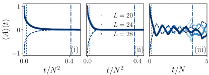
Figure 1: The expectation value $\langle A\rangle(t)$ of the coarse spin imbalance as a function of rescaled time for initial states $|\psi^{+}_{0}\rangle$ (solid line) and $|\psi^{-}_{0}\rangle$ (dashed line) for the chaotic (i), interacting integrable (ii) and non-interacting integrable (iii) cases. The dotted (dash-dotted) vertical line represents $T=T_{\text{neq}}$ ($T=T_{\text{eq}}$), where $T_{\text{neq}}$ indicates the time at which $\langle A\rangle(t)$ decays to $e^{-1}$ of its initial value and $T_{\text{eq}}=20T_{\text{neq}}$.

Since it is cumbersome to study $\epsilon(\boldsymbol{x};\boldsymbol{y})$ for every pair of histories $(\boldsymbol{x};\boldsymbol{y})$, we consider two quantities. First, we quantify the average amount of decoherence by

$$\overline{\epsilon}=\frac{1}{M^{2L-1}-M^{L}}\sum_{\boldsymbol{x}\neq\boldsymbol{y}}|\epsilon(\boldsymbol{x};\boldsymbol{y})|,$$ (6)

where $M^{2L-1}-M^{L}$ equals the number of non-trivial pairs $(\boldsymbol{x};\boldsymbol{y})$ (excluding those for which $\boldsymbol{x}=\boldsymbol{y}$ and $x_{n}\neq y_{n}$). Second, to capture the behaviour of statistical outliers we quantify the worst case scenario (the maximum coherence between histories) by

$$\epsilon_{\text{max}}=\max_{\boldsymbol{x}\neq\boldsymbol{y}}|\epsilon(\boldsymbol{x};\boldsymbol{y})|.$$ (7)

Model.—As a paradigmatic and non-trivial quantum many-body system we consider a XXZ Heisenberg spin chain with Hamiltonian

$$H=\sum_{\ell=1}^{N}\left(s_{x}^{\ell}s_{x}^{\ell+1}+s_{y}^{\ell}s_{y}^{\ell+1}+\Delta_{1}s_{z}^{\ell}s_{z}^{\ell+1}+\Delta_{2}s_{z}^{\ell}s_{z}^{\ell+2}\right),$$ (8)

where $s^{\ell}_{x,y,z}=\sigma^{\ell}_{x,y,z}/2$ are spin operators at lattice sites $\ell$, $N$ is the length of the chain, and we assume periodic boundary conditions. Crucial for our purposes is that Eq. (8) contains three classes of systems for different parameter regimes: (i) for $\Delta_{1}\neq 0\neq\Delta_{2}$ (we choose $\Delta_{1}=1.5$, $\Delta_{2}=0.5$) the model is non-integrable (or chaotic) meaning that nearest-level-spacing follows a Wigner-Dyson distribution [48], and it satisfies the eigenstate thermalization hypothesis [49, 50]; (ii) for $\Delta_{1}\neq 0$ but $\Delta_{2}=0$ (we choose $\Delta_{1}=1.5$) it is an interacting integrable model, which is solvable by Bethe ansatz [51]; (iii) for $\Delta_{1}=\Delta_{2}=0$ the model is non-interacting integrable (or free) and can be mapped to a quadratic Hamiltonian (a set of free fermions) via Jordan-Wigner and Bogoliubov transformation [52]. Note that the fact that (ii) is integrable but can not be mapped to free fermions like (iii) is crucial: it qualitatively influences its transport behavior [53], operator complexity [54] and, as we reveal below, its decoherence.

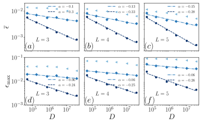
Figure 2: Average $\overline{\epsilon}$ and maximum $\epsilon_{\text{max}}$ amount of coherence versus Hilbert space dimension $D$ for the (i) chaotic (dark blue disks), (ii) interacting integrable (medium blue diamonds) and (iii) free (light blue triangles) case for $L\in\{3,4,5\}$. The dashed and dash-dotted line fit a scaling law of the form $D^{-\alpha}$ to (i) and (ii). The time step is $T=T_{\text{neq}}$ and the system sizes are $N=18,20,\dots,28$. Note the double-logarithmic scale.

As an interesting observable we study the spin-imbalance operator,

$$A_{0}=S_{z}^{L}-S_{z}^{R}=\sum_{\ell=1}^{\frac{N}{2}}s_{z}^{\ell}-\sum_{\ell=\frac{N}{2}+1}^{N}s_{z}^{\ell},$$ (9)

which quantifies a “magnetization bias” between the left and right half of the spin chain. Denoting its eigenvectors and eigenvalues by $A_{0}|a_{k}\rangle=a_{k}|a_{k}\rangle$, we construct a coarse observable $A=\Pi_{+}-\Pi_{-}$ with projectors

$$\Pi_{+}=\sum_{a_{k}\geq 0}|a_{k}\rangle\langle a_{k}|\quad\text{and}\quad\Pi_{-}=\sum_{a_{k}<0}|a_{k}\rangle\langle a_{k}|.$$ (10)

As the total magnetization $S_{z}=\sum_{\ell=1}^{N}s_{z}^{\ell}$ in $z$-direction commutes with $H$, we restrict the dynamics to a subspace with fixed $S_{z}$. We choose $S_{z}=0$ for system size $N=4k+2$ with resulting Hilbert space dimension $D=\binom{N}{2k+1}$ and $S_{z}=1$ for $N=4k$ with $D=\binom{N}{2k+2}$, where $k\in\mathbb{N}$. In this way, we ensure equal subspace dimensions $V_{+}=V_{-}$ with $V_{\pm}=\dim{\cal{H}}_{\pm}$.

An interesting consequence of these choices is that the spin imbalance $A_{0}=S_{z}^{L}-S_{z}^{R}$ can be determined by only measuring $S_{z}^{L}$ or $S_{z}^{R}$, owing to the conservation of $S_{z}=S_{z}^{L}+S_{z}^{R}$. Also owing to the conservation of $S_{z}$, the reduced density matrix of the left (right) half of the spin chain always commutes with $S_{z}^{L}$ ($S_{z}^{R}$), i.e., it is always block diagonal in the eigenbasis of $S_{z}^{L}$ ($S_{z}^{R}$). This is a consequence of symmetry and not of EID. Nevertheless, as we will see below, the histories are not exactly decoherent in that basis.

Numerical results.—To get an overall picture of the average dynamics we plot the expectation value $\langle A\rangle(t)$ of the coarse spin imbalance as a function of time in Fig. 1. This is done for two different non-equilibrium initial states $|\psi_{0}^{\pm}\rangle$, where $|\psi_{0}^{\pm}\rangle$ is a Haar random state restricted to the subspace ${\cal{H}}_{\pm}$. Remarkably, the behaviour in case (i) and (ii) agrees quantitatively: the system relaxes exponentially to its thermal equilibrium value $\langle A\rangle_{\text{eq}}=0$ with an equilibration time scale $\propto N^{2}$. In contrast, in case (iii) $\langle A\rangle(t)$ decays on a time scale $\propto N$ and fluctuates around $\langle A\rangle_{\text{eq}}$ without any clearly visible equilibration (up to the time that we considered).

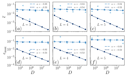
Figure 3: Identical to Fig. 2 except for time steps $T=T_{\text{eq}}$.

The emergence of classicality is investigated in Figs. 2 and 3 for Haar random initial states $|\psi_{0}\rangle$. We plot in double logarithmic scale $\overline{\epsilon}$ and $\epsilon_{\text{max}}$ versus the Hilbert space dimension $D$ for histories of lengths $L\in\{3,4,5\}$; the case $L=2$ has a universal typical decay owing to the Haar random nature of the initial state [20] as exemplified in the supplemental material (SM). The plots are obtained for constant time intervals $t_{k}-t_{k-1}=T$ for two different $T$: a nonequilibrium time scale $T_{\text{neq}}$ in Fig. 2 (identical to the dotted line in Fig. 1) and an equilibrium time scale $T_{\text{eq}}$ in Fig. 3 (identical to the dash-dotted line in Fig. 1). More precisely, $T_{\text{neq}}$ is defined as the time at which $\langle A\rangle(t)$ decays to $e^{-1}$ of its initial value [55] and the equilibrium time scale is defined as $T_{\text{eq}}=20T_{\text{neq}}$. While in the free model (iii) there is no clearly visible equilibration in Fig. 1, we use the same convention for $T_{\text{eq}}$ for better comparison. Finally, each data point in Figs. 2 and 3 is obtained by averaging $\overline{\epsilon}$ and $\epsilon_{\text{max}}$ over $2^{30-N}$ different realizations of $|\psi_{0}\rangle$. In the SM we show that the variance of $\overline{\epsilon}$ and $\epsilon_{\text{max}}$ decays as $D^{-1}$ for all three cases (i), (ii) and (iii) (likely as a consequence of dynamical typicality [56, 57]), which justifies our focus on the average behaviour.

We then observe in Figs. 2 and 3 the following (an explanation follows later). First, for the chaotic case (i) we find a scaling law of the form $D^{-\alpha}$ (note that $D$ scales exponentially with the number of spins $N$) with $\alpha\approx 0.35$ ($\alpha\approx 0.25$) for $\overline{\epsilon}$ ($\epsilon_{\text{max}}$) at the nonequilibrium time scale and with $\alpha\approx 0.5$ for both $\overline{\epsilon}$ and $\epsilon_{\text{max}}$ at the equilibrium time scale. This indicates a robust exponential suppression (with respective to system size $N$) of coherences in chaotic systems. For the interacting integrable case (ii) we find three major differences compared to (i). First, we can safely conclude that the exponent $\alpha$ is smaller in all cases. Second, for $T_{\text{eq}}$ $\alpha$ is smaller than for $T_{\text{neq}}$, conversely to case (i). Indeed, for $T_{\text{eq}}$ (Fig. 3) we even find $\alpha\approx 0$, indicating a possible sub-exponential or power-law suppression (with respect to $N$) of coherences. Third, the exponent $\alpha$ for $\epsilon_{\text{max}}$ is roughly half the magnitude than $\alpha$ for $\overline{\epsilon}$ at $T_{\text{neq}}$, indicating stronger fluctuations in the DF among different pairs $(\boldsymbol{x};\boldsymbol{y})$ of histories. Finally, the free case (iii) is characterized for $T_{\text{neq}}$ by much larger coherences and for $T_{\text{eq}}$ by strong fluctuations among different $N$, making it unjustified to even speak of any scaling law $D^{-\alpha}$.

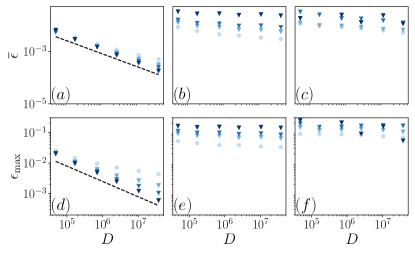
Figure 4: Average $\overline{\epsilon}$ and maximum $\epsilon_{\text{max}}$ amount of coherence versus Hilbert space dimension $D$ for history length $L=5$ for chaotic (a,d), interacting integrable (b,e) and non-interacting integrable (c,f) cases for time steps $T=T_{\text{neq}},2T_{\text{neq}},3T_{\text{neq}},T_{\text{eq}}$ (from light to dark blue). The dashed line indicate the scaling $D^{-1/2}$. The system size is $N=18,20,\dots,28$.

A particularly intriguing observation is the distinctive behaviour of decoherence as a function of $T$, which is further studied in Fig. 4. Whereas in case (i) $\overline{\epsilon}$ and $\epsilon_{\text{max}}$ consistently decrease and the exponent grows to $\alpha\approx 0.5$ for increasing $T$, the opposite happens for case (ii): decoherence becomes consistently weaker for larger $T$ and no exponential scaling is visible anymore for $\epsilon_{\text{max}}$ at $T_{\text{eq}}$. Finally, for case (iii) no clear pattern is visible and the large fluctuations make it difficult to speak of any scaling at all.

Explanation.—We start by noting that there is some consensus about the qualitative origin of decoherence (whether in the histories or EID framework), namely that coarse and slow (or “quasi-conserved”) observables of many-body systems behave classical. However, other qualitative questions (e.g., is non-integrability essential or not?) have not been addressed in the past, and useful estimates of the DF are hard to obtain in general [20, 21]. Nevetherless, it seems that al least a transparent explanation for the quantitative behaviour of the DF for chaotic systems can be given.

To this end, recall that the overlap $\langle\phi|\chi\rangle$ between two Haar random vectors $|\phi\rangle$ and $|\chi\rangle$ scales like $1/\sqrt{D}$ and that the subspace dimensions $V_{x}$ are proportional to $D$ for many relevant coarse-grainings. Thus, for equilibrium time scales $T_{\text{eq}}$ the history states $|\psi(\boldsymbol{x})\rangle$ in a chaotic system behave like randomly drawn typical states because they had time to explore the available Hilbert space in an unbiased way owing to the absence of conserved quantities (besides energy). Now, for nonequilibrium time scales $T_{\text{neq}}$ the history states $|\psi(\boldsymbol{x})\rangle$ will not look fully randomized as they contain further information compared to the equilibrium case. Therefore, the exponent $\alpha=\alpha(T)$ is expected to grow with $T$ until it reaches $\alpha(T)\approx 0.5$ for $T\gtrsim T_{\text{eq}}$. Which values it takes precisely is, however, determined by $H$, $\{\Pi_{x}\}$ and $|\psi_{0}\rangle$ in a complicated way.

Unfortunatey, it seems much more complicated to explain the behaviour for cases (ii) and (iii). Certainly, owing to the extensive number of conserved quantities, the states $|\psi(\boldsymbol{x})\rangle$ can not explore the available Hilbert space in an unbiased fashion, which causes deviations from the behaviour of typical states. Yet, why the exponent $\alpha(T)$ becomes even smaller for larger $T$ remains a mystery. A speculative guess could be that at short time scales the dynamics is governed by time-dependent perturbation theory (Fermi’s golden rule), which is more determined by the rough structure of the spectrum of the Hamiltonian. At long times, instead, the fine structure of the Hamiltonian (its conserved quantities) become increasingly important for the dynamical behaviour.

Conclusion.—We numerically extracted finite size scaling laws for the DF of a realistic quantum many-body system in an approximation-free way and we revealed decisive differences depending on the nature of the system. The chaotic case (i) showed a strong and robust emergence of decoherence in contrast to the interacting integrable case (ii) with a quantitatively much weaker form of decoherence. Note that this difference could not have been guessed from the quantitatively almost identical single-time behaviour shown in Fig. 1. A qualitative even weaker form of decoherence was observed for free models (iii), making it even hard to speak of any definite signature of decoherence, even though our finite size calculations do not directly invalidate conclusions obtained from free models in the thermodynamic limit [5, 6, 7, 8, 10, 11, 12]. In particular, for another model (energy exchanges in an Ising chain, studied in the SM) we found a clear signature of decoherence also for the free case (while still being much weaker compared to the chaotic case).

Our findings motivate the conjecture that the normalized DF in Eq. (5) can be written in the chaotic case for slow and coarse observables as

$$\epsilon(\boldsymbol{x};\boldsymbol{y})=\frac{r_{\boldsymbol{x},\boldsymbol{y}}}{D^{\alpha}}\leavevmode\nobreak\ \leavevmode\nobreak\ \leavevmode\nobreak\ \text{for }\boldsymbol{x}\neq\boldsymbol{y}.$$ (11)

Here, $D^{-\alpha}$ describes the overall scaling with an exponent $\alpha$ that depends on many details (initial state, considered time interval, etc.) but is often not much smaller than $0.5$. Moreover, the coefficients $r_{\boldsymbol{x},\boldsymbol{y}}$ are of order one and do not depend on $D$. While they are in principle determined by $H$, $\{\Pi_{x}\}$ and $|\psi_{0}\rangle$, they depend on so many experimentally uncontrollable microscopic parameters such that they appear erratic and unpredictable (similar to the off-diagonal elements in the eigenstate thermalization hypothesis [49, 50]), a point that we further support in the SM. The conjecture (11) is in unison with previous analytical estimates [20, 21] and scaling laws [22], and it breaks down when the number of histories $M^{L}$ becomes of the order of the Hilbert space dimension $D$ [23].

Outlook.—Our results motivate further research in various directions. On a quantitative level, for instance, it remains open to understand the precise behaviour of $\alpha(T)$ (and in particular the peculiarities of integrable models) as well as the effect of long histories with $L\gg 1$, which was numerically inaccessible to us. On a qualitative level, it would be intriguing to find out whether other classes of systems (e.g., disordered or localized systems) and phases of matter (e.g., close to criticality or topological phases) also have such a strong influence on the behaviour of decoherence as seen here.

Acknowledgement.—JW is financially supported by the Deutsche Forschungsgemeinschaft (DFG), under Grant No. 531128043, as well as under Grant No. 397107022, No. 397067869, and No. 397082825 within the DFG Research Unit FOR 2692, under Grant No. 355031190. PS is financially supported by “la Caixa” Foundation (ID 100010434, fellowship code LCF/BQ/PR21/11840014) as well as the MICINN with funding from European Union NextGenerationEU (PRTR-C17.I1), by the Generalitat de Catalunya (project 2017-SGR-1127), the European Commission QuantERA grant ExTRaQT (Spanish MICIN project PCI2022-132965), and the Spanish MINECO (project PID2019-107609GB-I00) with the support of FEDER funds. Additionally, we greatly acknowledge computing time on the HPC3 at the University of Osnabrück, granted by the DFG, under Grant No. 456666331.

Supplemental material

We here report on further numerical results that strengthen our main message. We start by supplementing additional results for the XXZ Heisenberg chain studied in the main text (subsection S1), continued by comparing the chaotic and free case for energy exchanges in an Ising chain (subsection S2), and finally we look at the level statistics to demonstrate that our models are chaotic (subsection S3).

.1 S1. Additional numerical results in XXZ model

We begin by showing plots similar to Figs. 2 and 3 in the main text, but for time-interval $T=2T_{\text{neq}}$ and $T=3T_{\text{neq}}$. Since $T_{\text{neq}}<T<T_{\text{eq}}$, we expect that Figs. S1 and S2 interpolates between the conclusions we obtained from Figs. 2 and 3, which is indeed the case. We find a stronger exponential suppression of decoherence for case (i) and a weaker exponential suppression for case (ii). Interestingly, the magnitude of decoherence for case (iii) is similar to case (ii) in contrast to Fig. 2, but it starts to fluctuate more, making a fit to a scaling law $D^{-\alpha}$ unreasonable as in Fig. 3.

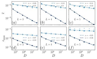
Figure S1: Identical to Figs. 2 and 3 in the main text except for time steps $T=2T_{\text{neq}}$.

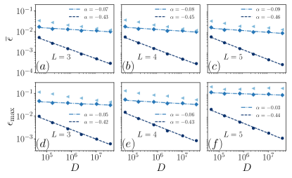
Figure S2: Identical to Figs. 2 and 3 in the main text except for time steps $T=3T_{\text{neq}}$.

In Fig. S3 we display $\overline{\epsilon}$ and $\epsilon_{\text{max}}$ for the shortest possible non-trivial history with length $L=2$. As claimed in the main mansuscript, we observe consistently a $D^{-0.5}$ scaling in all three cases (i), (ii) and (iii). This effect is due to the Haar random choice of the initial state and the fact that the Haar measure is invariant under unitary transformations. Thus, the first unitary time evolution $U_{1,0}$ is barely able to change the decoherence properties of the system.

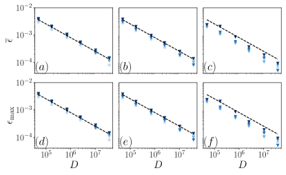
Figure S3: $\overline{\epsilon}$ and $\epsilon_{\text{max}}$ versus Hilbert space dimension $D$ for $L=2$, for chaotic (a,d), interacting integrable (b,e) and non-interacting integrable (c,f) cases for time steps $T=T_{\text{neq}},2T_{\text{neq}},3T_{\text{neq}},T_{\text{eq}}$ (from light to dark). The dashed line indicates the scaling $D^{-0.5}$ as a guidance to the eyes.

Next, we consider the variance of $\overline{\epsilon}$ and $\epsilon_{\text{max}}$ for $T_{\text{neq}}$ in Fig. S4 and $T_{\text{eq}}$ in Fig. S5. This is extracted from a histogram of the $2^{30-N}$ different realizations of $|\psi_{0}\rangle$. As we can see in all three cases (i), (ii) and (iii), the variance is orders of magnitude smaller than the mean and scales roughly like $1/D$, likely as a consequence of dynamical typicality. This is the reason why we can focus on the averaged values in the main text.

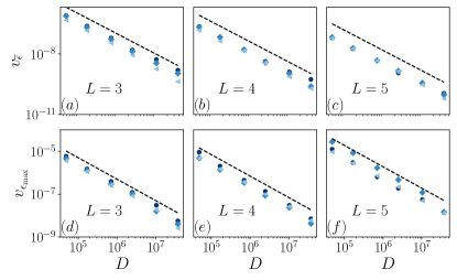
Figure S4: Variance of $\overline{\epsilon}$ and $\epsilon_{\text{max}}$ versus Hilbert space dimension $D$ for cases (i) (dark blue disks), (ii) (medium blue diamonds) and (iii) (light blue triangles) for $L=3,4,5$. The dashed line indicates the scaling $\propto D^{-1}$. The time step is $T=T_{\text{neq}}$ and the system sizes are $N=18,20,\dots,28$.

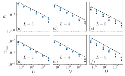
Figure S5: Similar to Fig. S4 but for the time scale $T=T_{\text{eq}}$.

Furthermore, we directly compare in Fig. S6 how the average $\overline{\epsilon}$ and maximum $\epsilon_{\text{max}}$ coherence changes as a function of $L$ for the chaotic case. We observe an almost constant behaviour for $\overline{\epsilon}$ if $T=T_{\text{eq}}$ and only some mild changes for $T_{\text{neq}}$, which could be a result of the finite amount of samples. For $\epsilon_{\text{max}}$ instead we consistenly observe (slightly) larger values for larger $L$ for both $T_{\text{eq}}$ and $T_{\text{neq}}$. This is most likely caused by the fact that the DF has more entries for larger $L$ (the number of non-trivial entries grows like $M^{2L-1}-M^{L}$). Since $\epsilon_{\text{max}}$ was defined to measure statistical outliers, it is clear that there are bigger chances for stronger deviations if there are more elements to sample from.

In addition to the averaged and maximum value of $\epsilon_{\boldsymbol{x},\boldsymbol{y}}$, we also study its distribution. As an example, in Fig. S7, we show the distribution of the real and imaginary part of $\epsilon_{\boldsymbol{x},\boldsymbol{y}}$ for $N=20,\ L=5,\ T=T_{\text{eq}}$, where we exclude pairs of $\boldsymbol{x},\boldsymbol{y}$ for which $x_{n}\neq y_{n}$ or $x_{0}\neq y_{0}$. Data from $2^{10}$ different initial random states are taken into account. In the chaotic case (i), a similar shape of distribution is found for the real ($f_{R}(\epsilon)$) and imaginary part ($f_{I}(\epsilon)$). However, slight deviations are clearly observed, especially in the variance (second moments), indicating that $\epsilon_{\boldsymbol{x},\boldsymbol{y}}$ can not be random numbers in a strict sense. This is due to the fact that in a real system, starting from the same initial state, different histories are nevertheless correlated. However, in comparison with the integrable cases (ii) and (iii), where we observe large deviations between $f_{R}(\epsilon)$ and $f_{I}(\epsilon)$, the correlations in the chaotic case are almost negligible.

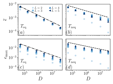
Figure S6: $\overline{\epsilon}$ and $\epsilon_{\text{max}}$ versus Hilbert space dimension $D$ for the chaotic case (i) for $L\in\{3,4,5\}$. The time step is $T={T_{\text{eq}}}$ in (a,c) and $T=T_{\text{neq}}$ in (b,d). The dashed-dotted (dashed) line indicates the $\sim D^{-0.5}$ ($\sim D^{-0.3}$) scaling as a guidance to the eyes.

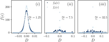
Figure S7: Distribution of real ($f_{R}(\epsilon)$) and imaginary ($f_{I}(\epsilon)$) part of ${\epsilon}_{\boldsymbol{x},\boldsymbol{y}}$ in the XXZ model for $N=20$, $L=5$ and $T=T_{\text{eq}}$ for (i) chaotic; (ii) interacting integrable and (iii) free cases. $\sigma_{R,I}$ indicates the standard variance of $f_{R,I}(\epsilon)$.

S2. Numerical results in Ising model

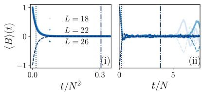
Figure S8: The expectation value $\langle B\rangle(t)$ of the coarse energy imbalance in the Ising model as a function of rescaled time for initial states $|\psi^{+}_{0}\rangle$ (solid line) and $|\psi^{-}_{0}\rangle$ (dashed line) for chaotic (i) and free (ii) cases. The dotted (dash-dotted) vertical line represents $T=T_{\text{neq}}$ ($T=T_{\text{eq}}$), where $T_{\text{neq}}$ indicates the time at which $\langle B\rangle(t)$ decays to $e^{-1}$ of its initial value and $T_{\text{eq}}=20T_{\text{neq}}$.

To analyze the generality of our main results, we also consider an Ising chain with Hamiltonian

$$H=\sum_{\ell=1}^{N}\left(h_{x}\sigma_{x}^{\ell}+h_{z}\sigma_{z}^{\ell}+J\sigma_{z}^{\ell}\sigma_{z}^{\ell}\right).$$ (S1)

We assume periodic boundary condition and set $J=h_{x}=1.0$. Two different values of $h_{z}$ are considered: (i) for $h_{z}=0.5$ (titled field) the system is chaotic; (ii) for $h_{z}=0.0$ (transverse field) the system is integrable and can be mapped to free fermions. A natural operator of interest here is an energy imbalance operator,

$$B_{0}=H^{L}-H^{R},$$ (S2)

where

$$H^{L}=\sum_{\ell=1}^{\frac{N}{2}}(h_{x}\sigma_{x}^{\ell}+h_{z}\sigma_{z}^{\ell})+\sum_{\ell=1}^{\frac{N}{2}-1}J\sigma_{z}^{\ell}\sigma_{z}^{\ell+1},$$

$$H^{R}=\sum_{\ell=\frac{N}{2}+1}^{N}(h_{x}\sigma_{x}^{\ell}+h_{z}\sigma_{z}^{\ell})+\sum_{\ell=\frac{N}{2}-1}^{N-1}J\sigma_{z}^{\ell}\sigma_{z}^{\ell+1}.$$ (S3)

It quantifies an “energy bias” between the left and right half of the spin chain. Denoting its eigenvectors and eigenvalues by $B_{0}|b_{k}\rangle=b_{k}|b_{k}\rangle$, we construct a coarse observable $B=\Pi^{B}_{+}-\Pi^{B}_{-}$ with projectors

$$\Pi^{B}_{+}=\sum_{b_{k}\geq 0}|b_{k}\rangle\langle b_{k}|\quad\text{and}\quad\Pi^{B}_{-}=\sum_{b_{k}<0}|b_{k}\rangle\langle b_{k}|.$$ (S4)

The subspaces are denoted by ${\cal H}^{B}_{\pm}$, with Hilbert space dimension $V^{B}_{\pm}=\text{dim}{\cal H^{B}_{\pm}}=\text{Tr}[\Pi^{B}_{\pm}]$. In this model, $V^{B}_{+}\approx V^{B}_{-}$.

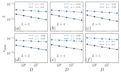
Figure S9: Average $\overline{\epsilon}$ and maximum $\epsilon_{\text{max}}$ amount of coherence versus Hilbert space dimension $D$ in Ising model for the (i) chaotic (dark blue disks) and (ii) interacting integrable (medium blue diamonds) case. The dashed and dash-dotted line fit a scaling law of the form $D^{-\alpha}$ to (i) and (ii). The time step is $T=T_{\text{neq}}$ and the system sizes are $N=18,20,\dots,26$.

As a start, we plot the expectation value $\langle B\rangle(t)$ of the coarse energy imbalance as a function of time in Fig. S8. This is done for two different non-equilibrium initial states $|\psi_{0}^{\pm}\rangle$, where $|\psi_{0}^{\pm}\rangle$ is a Haar random state restricted to the subspace ${\cal{H}}^{B}_{\pm}$. In the chaotic case (i) the system relaxes to its thermal equilibrium value $\langle B\rangle_{\text{eq}}=0$ with an equilibration time scale $\propto N^{2}$. In contrast, in the free case (ii) $\langle B\rangle(t)$ decays on a time scale $\propto N$ and fluctuates around $\langle B\rangle_{\text{eq}}$ without any clearly visible equilibration (up to the time that we considered). Note, however, that—compared to the free case of the Heisenberg chain considered in the main text [cf. Fig. 1]—equilibration seems to work much better for the free case of the Ising model.

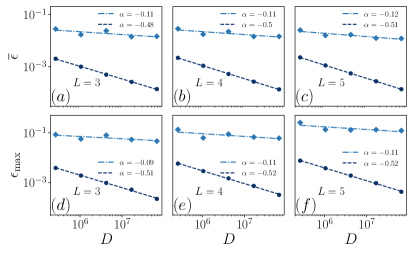
Figure S10: Identical to Fig. S9 except for time steps $T=T_{\text{eq}}$.

The emergence of decoherence is investigated in Figs. S9 and S10 for Haar random initial states $|\psi_{0}\rangle$. We plot in double logarithmic scale $\overline{\epsilon}$ and $\epsilon_{\text{max}}$ versus the Hilbert space dimension $D$ for histories of lengths $L\in\{3,4,5\}$ for two different $T$: a nonequilibrium time scale $T_{\text{neq}}$ in Fig. S9 (identical to the dotted line in Fig. S8) and an equilibrium time scale $T_{\text{eq}}$ in Fig. S10 (identical to the dash-dotted line in Fig. S8). Finally, each data point in Figs. S9 and S10 is obtained by averaging $\overline{\epsilon}$ and $\epsilon_{\text{max}}$ over $2^{28-N}$ different realizations of $|\psi_{0}\rangle$.

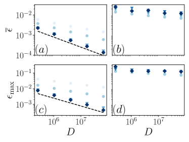
Figure S11: Average $\overline{\epsilon}$ and maximum $\epsilon_{\text{max}}$ amount of coherence versus Hilbert space dimension $D$ for history length $L=5$ in the Ising model for chaotic (a,c) and non-interacting integrable (b,d) cases for time steps $T=0.5T_{\text{neq}},T_{\text{neq}},2T_{\text{neq}},3T_{\text{neq}},T_{\text{eq}}$ (from light to dark blue). The dashed line indicate the scaling $\sim D^{-1/2}$. The system size $N=18,20,\dots,26$.

For the chaotic case (i) we find a scaling law of the form $D^{-\alpha}$ (note that $D\propto 2^{N}$) with $\alpha\approx 0.3$ at the nonequilibrium time scale and with $\alpha\approx 0.5$ at the equilibrium time scale (with the same $\alpha$ for both $\overline{\epsilon}$ and $\epsilon_{\text{max}}$). This again indicates a robust exponential suppression (with respective to system size $N$) of coherences in chaotic systems. For the non-interacting integrable case (ii) we find smaller exponents $\alpha\approx 0.1$ in all cases, yet it is remarkable compared to the free case of the Heisenberg chain studied in the main text that there seemingly is a scaling law. This illustrates how subtle the emergence of decoherence depends on the model under study and a possible reason for this descrepancy could also be the structure of the observable itself instead of the considered model.

The behaviour of decoherence as a function of $T$, is further studied in Fig. S11. For chaotic case (i) $\overline{\epsilon}$ and $\epsilon_{\text{max}}$ consistently decrease and the exponent grows to $\alpha\approx 0.5$ for increasing $T$. In contrast, for integrable case (ii), decoherence becomes (approximately) weaker for larger $T$, but it is again not as clear as for the example of the main text.

To summarize, in the Ising model we find again a strong difference between the chaotic and integrable case in terms of the finite size scaling of $\overline{\epsilon}$ and $\epsilon_{\text{max}}$ and their behavior as a function of $T$. This is qualitatively in unison with what we found in the main text and for the chaotic case it is even quantitatively in unison. However, we also found that the free case in the Ising model displays a much stronger form of decoherence compared to the free case in the Heisenberg model, showing that much care is required when one wants to generalize conclusions obtained for one specific integrable model.

S3. Level statistics

The study the chaocity (integrability) of the considered models, we analyze the distribution of the nearest-level spacing of the unfolded spectrum. After unfolding, the averaged level density becomes constant (usually set to $1$, as is done here). The ordered eigenvalues of the unfolded spectrum are denoted by $\tilde{E}_{i}$. As an indicator of quantum chaos, we study the distribution of $s_{i}=\tilde{E}_{i+1}-\tilde{E}_{i}$, denoted by $P(s)$. $P(s)$ differentiates between chaotic and integrable systems: i) For chaotic systems, $P(s)$ follows a Wigner-Dyson distribution, where for systems with time-reversal symmetry,

$$P(s)=P_{\text{GOE}}(s)=\frac{\pi}{2}se^{-\frac{\pi}{4}s^{2}},$$ (S5)

which is the prediction of Gaussian Orthogonal Ensemble (GOE); ii) For integrable systems, $P(s)$ follows a Poisson distribution

$$P(s)=P_{\text{Poisson}}(s)=e^{-s}\ .$$ (S6)

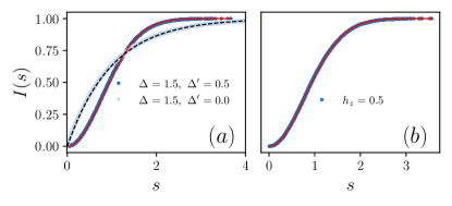
Figure S12: Level statistics: cumulative distribution of the nearest-level spacing $I(s)$ versus $s$, for (a) XXZ model ($N=24$) and (b) Ising model ($N=20$). The solid and dashed line indicates $I_{\text{GOE}}(s)$ and $I_{\text{Poisson}}(s)$, respectively (Eq. (S8)).

In practise, we consider the cumulative distribution of $P(s)$

$$I(s)=\int_{0}^{s}P(r)dr,$$ (S7)

and compare it to

$$I_{\text{GOE}}(s)=1-\exp{(-\frac{\pi}{4}s^{2})},\ I_{\text{Poisson}}(s)=1-\exp{(-s)}.$$ (S8)

In both models, due to the existence of additional global symmetries (e.g., translational invariance, reflection, et al.) alongside with the total energy, our analysis is confined to a specific subspace. We compute the $P(s)$ by considering $1/2$ of the total eigenvalues located in the middle of the spectrum, and results are shown in Fig. S12. Good agreement with the Wigner-Dyson distribution is observed in the XXZ model ($\Delta_{1}=1.5,\ \Delta_{2}=0.5$) and in the Ising model ($h_{z}=0.5$), indicating the systems are chaotic with respect to the corresponding parameter. In contrast, in XXZ model ($\Delta_{1}=1.5,\ \Delta_{2}=0.0$), a Possion distribution is found, which suggests that the system is integrable. The results are in line with our findings in the main text. The results for trivial cases, where the model is equivalent to free fermions, e.g., XXZ model ($\Delta_{1}=\Delta_{2}=0$) and Ising model $(h_{z}=0.0)$, are not shown here.

References

- Gell-Mann and Hartle [1990] M. Gell-Mann and J. B. Hartle, Complexity, Entropy and the Physics of Information (Reading: Addison-Wesley, 1990) Chap. Quantum Mechanics in the Light of Quantum Cosmology, pp. 425–459.
- Omnès [1992] R. Omnès, Consistent interpretations of quantum mechanics, Rev. Mod. Phys. 64, 339 (1992).
- Halliwell [1995] J. J. Halliwell, A Review of the Decoherent Histories Approach to Quantum Mechanics, Ann. (N.Y.) Acad. Sci. 755, 726 (1995).
- Dowker and Kent [1996] F. Dowker and A. Kent, On the consistent histories approach to quantum mechanics, J. Stat. Phys. 82, 10.1007/BF02183396 (1996).
- Schmid [1987] A. Schmid, Repeated measurements on dissipative linear quantum systems, Ann. Phys. 173, 103 (1987).
- Dowker and Halliwell [1992] H. F. Dowker and J. J. Halliwell, Quantum mechanics of history: The decoherence functional in quantum mechanics, Phys. Rev. D 46, 1580 (1992).
- Gell-Mann and Hartle [1993] M. Gell-Mann and J. B. Hartle, Classical equations for quantum systems, Phys. Rev. D 47, 3345 (1993).
- Halliwell [1999] J. J. Halliwell, Somewhere in the universe: Where is the information stored when histories decohere?, Phys. Rev. D 60, 105031 (1999).
- Brun and Hartle [1999] T. A. Brun and J. B. Hartle, Classical dynamics of the quantum harmonic chain, Phys. Rev. D 60, 123503 (1999).
- Halliwell [2001] J. J. Halliwell, Approximate decoherence of histories and ’t Hooft’s deterministic quantum theory, Phys. Rev. D 63, 085013 (2001).
- Subaşı and Hu [2012] Y. Subaşı and B. L. Hu, Quantum and classical fluctuation theorems from a decoherent histories, open-system analysis, Phys. Rev. E 85, 011112 (2012).
- Halliwell [2003] J. J. Halliwell, Decoherence of histories and hydrodynamic equations for a linear oscillator chain, Phys. Rev. D 68, 025018 (2003).
- [13] In this paper we numerically integrate the Schrödinger equation using the Chebyshev polynomial algorithm [58, 59] until convergence is reached.
- Van Kampen [1954] N. Van Kampen, Quantum statistics of irreversible processes, Physica 20, 603 (1954).
- Brun and Halliwell [1996] T. A. Brun and J. J. Halliwell, Decoherence of hydrodynamic histories: A simple spin model, Phys. Rev. D 54, 2899 (1996).
- Gemmer and Steinigeweg [2014] J. Gemmer and R. Steinigeweg, Entropy increase in -step Markovian and consistent dynamics of closed quantum systems, Phys. Rev. E 89, 042113 (2014).
- Schmidtke and Gemmer [2016] D. Schmidtke and J. Gemmer, Numerical evidence for approximate consistency and Markovianity of some quantum histories in a class of finite closed spin systems, Phys. Rev. E 93, 012125 (2016).
- Nation and Porras [2020] C. Nation and D. Porras, Taking snapshots of a quantum thermalization process: Emergent classicality in quantum jump trajectories, Phys. Rev. E 102, 042115 (2020).
- Albrecht et al. [2022] A. Albrecht, R. Baunach, and A. Arrasmith, Einselection, equilibrium, and cosmology, Phys. Rev. D 106, 123507 (2022).
- Strasberg et al. [2023a] P. Strasberg, A. Winter, J. Gemmer, and J. Wang, Classicality, Markovianity, and local detailed balance from pure-state dynamics, Phys. Rev. A 108, 012225 (2023a).
- Strasberg [2023] P. Strasberg, Classicality with(out) decoherence: Concepts, relation to Markovianity, and a random matrix theory approach, SciPost Phys. 15, 024 (2023).
- Strasberg et al. [2023b] P. Strasberg, T. E. Reinhard, and J. C. Schindler, Everything Everywhere All At Once: A First Principles Numerical Demonstration of Emergent Decoherent Histories, arXiv: 2304.10258 (2023b).
- Strasberg and Schindler [2023] P. Strasberg and J. Schindler, Shearing Off the Tree: Emerging Branch Structure and Born’s Rule in an Equilibrated Multiverse, arXiv: 2310.06755 (2023).
- Arrasmith et al. [2019] A. Arrasmith, L. Cincio, A. T. Sornborger, W. H. Zurek, and P. J. Coles, Variational consistent histories as a hybrid algorithm for quantum foundations, Nature communications 10, 3438 (2019).
- Joos et al. [2003] E. Joos, H. D. Zeh, C. Kiefer, D. Giulini, J. Kupsch, and I.-O. Stamatescu, Decoherence and the Appearance of a Classical World in Quantum Theory (Springer, Berlin Heidelberg, 2003).
- Zurek [2003] W. H. Zurek, Decoherence, einselection, and the quantum origins of the classical, Rev. Mod. Phys. 75, 715 (2003).
- Schlosshauer [2019] M. Schlosshauer, Quantum decoherence, Phys. Rep. 831, 1 (2019).
- Kiefer [1991] C. Kiefer, Interpretation of the decoherence functional in quantum cosmology, Class. Quant. Grav. 8, 379 (1991).
- Albrecht [1992] A. Albrecht, Investigating decoherence in a simple system, Phys. Rev. D 46, 5504 (1992).
- Finkelstein [1993] J. Finkelstein, Definition of decoherence, Phys. Rev. D 47, 5430 (1993).
- Paz and Zurek [1993] J. P. Paz and W. H. Zurek, Environment-induced decoherence, classicality, and consistency of quantum histories, Phys. Rev. D 48, 2728 (1993).
- Riedel et al. [2016] C. J. Riedel, W. H. Zurek, and M. Zwolak, Objective past of a quantum universe: Redundant records of consistent histories, Phys. Rev. A 93, 032126 (2016).
- Gorin et al. [2006] T. Gorin, T. Prosen, T. H. Seligman, and M. Žnidarič, Dynamics of Loschmidt echoes and fidelity decay, Phys. Rep. 435, 33 (2006).
- Swingle [2018] B. Swingle, Unscrambling the physics of out-of-time-order correlators, Nat. Phys. 14, 988 (2018).
- Milz and Modi [2021] S. Milz and K. Modi, Quantum Stochastic Processes and Quantum non-Markovian Phenomena, PRX Quantum 2, 030201 (2021).
- Cucchietti et al. [2003] F. M. Cucchietti, D. A. R. Dalvit, J. P. Paz, and W. H. Zurek, Decoherence and the Loschmidt Echo, Phys. Rev. Lett. 91, 210403 (2003).
- Kitaev [2015] A. Kitaev, A simple model of quantum holography (KITP 2015, 2015).
- Maldacena et al. [2016] J. Maldacena, S. H. Shenker, and D. Stanford, A bound on chaos, J. High Energy Phys. 2016, 106.
- Rozenbaum et al. [2017] E. B. Rozenbaum, S. Ganeshan, and V. Galitski, Lyapunov exponent and out-of-time-ordered correlator’s growth rate in a chaotic system, Phys. Rev. Lett. 118, 086801 (2017).
- Murthy and Srednicki [2019] C. Murthy and M. Srednicki, Bounds on Chaos from the Eigenstate Thermalization Hypothesis, Phys. Rev. Lett. 123, 230606 (2019).
- Xu et al. [2020] T. Xu, T. Scaffidi, and X. Cao, Does Scrambling Equal Chaos?, Phys. Rev. Lett. 124, 140602 (2020).
- Sánchez et al. [2022] C. M. Sánchez, A. K. Chattah, and H. M. Pastawski, Emergent decoherence induced by quantum chaos in a many-body system: A Loschmidt echo observation through NMR, Phys. Rev. A 105, 052232 (2022).
- Dowling et al. [2023] N. Dowling, P. Kos, and K. Modi, Scrambling Is Necessary but Not Sufficient for Chaos, Phys. Rev. Lett. 131, 180403 (2023).
- Dowling and Modi [2024] N. Dowling and K. Modi, Operational metric for quantum chaos and the corresponding spatiotemporal-entanglement structure, PRX Quantum 5, 010314 (2024).
- Griffiths [1984] R. B. Griffiths, Consistent histories and the interpretation of quantum mechanics, J. Stat. Phys. 36, 219 (1984).
- Hartle [2016] J. B. Hartle, Decoherent Histories Quantum Mechanics Starting with Records of What Happens, arXiv 1608.04145 (2016).
- Szańkowski and Cywiński [2023] P. Szańkowski and L. Cywiński, Objectivity of classical quantum stochastic processes, arXiv: 2304.07110 (2023).
- Richter et al. [2020] J. Richter, A. Dymarsky, R. Steinigeweg, and J. Gemmer, Eigenstate thermalization hypothesis beyond standard indicators: Emergence of random-matrix behavior at small frequencies, Phys. Rev. E 102, 042127 (2020).
- D’Alessio et al. [2016] L. D’Alessio, Y. Kafri, A. Polkovnikov, and M. Rigol, From quantum chaos and eigenstate thermalization to statistical mechanics and thermodynamics, Adv. Phys. 65, 239 (2016).
- Deutsch [2018] J. M. Deutsch, Eigenstate thermalization hypothesis, Rep. Prog. Phys. 81, 082001 (2018).
- Bethe [1931] H. Bethe, Zur Theorie der Metalle: I. Eigenwerte und Eigenfunktionen der linearen Atomkette, Zeitschrift für Physik 71, 205 (1931).
- Sachdev [2011] S. Sachdev, Quantum Phase Transitions, 2nd ed. (Cambridge University Press, 2011).
- Bertini et al. [2021] B. Bertini, F. Heidrich-Meisner, C. Karrasch, T. Prosen, R. Steinigeweg, and M. Žnidarič, Finite-temperature transport in one-dimensional quantum lattice models, Rev. Mod. Phys. 93, 025003 (2021).
- Parker et al. [2019] D. E. Parker, X. Cao, A. Avdoshkin, T. Scaffidi, and E. Altman, A universal operator growth hypothesis, Phys. Rev. X 9, 041017 (2019).
- [55] Specifically, we obtain from the data of the largest system size . Then, for smaller sizes we set with for (i) and (ii) and for (iii).
- Reimann and Gemmer [2020] P. Reimann and J. Gemmer, Why are macroscopic experiments reproducible? Imitating the behavior of an ensemble by single pure states, Physica A 552, 121840 (2020).
- Teufel et al. [2023] S. Teufel, R. Tumulka, and C. Vogel, Time Evolution of Typical Pure States from a Macroscopic Hilbert Subspace, J. Stat. Phys. 190, 69 (2023).
- De Raedt et al. [2007] K. De Raedt, K. Michielsen, H. De Raedt, B. Trieu, G. Arnold, M. Richter, T. Lippert, H. Watanabe, and N. Ito, Massively parallel quantum computer simulator, Computer Physics Communications 176, 121 (2007).
- Jin et al. [2010] F. Jin, H. De Raedt, S. Yuan, M. I. Katsnelson, S. Miyashita, and K. Michielsen, Approach to equilibrium in nano-scale systems at finite temperature, Journal of the Physical Society of Japan 79, 124005 (2010).