MS-0001-1922.65

Liao and Kroer

Statistical Inference in Market Equilibrium

Statistical Inference and A/B Testing in Fisher Markets and Paced Auctions

Luofeng Liao Department of Industrial Engineering and Operations Research, Columbia University, ll3530@columbia.edu Christian Kroer Department of Industrial Engineering and Operations Research, Columbia University, ck2945@columbia.edu

We initiate the study of statistical inference and A/B testing for two market equilibrium models: linear Fisher market (LFM) equilibrium and first-price pacing equilibrium (FPPE). LFM arises from fair resource allocation systems such as allocation of food to food banks and notification opportunities to different types of notifications. For LFM, we assume that the data observed is captured by the classical finite-dimensional Fisher market equilibrium, and its steady-state behavior is modeled by a continuous limit Fisher market. The second type of equilibrium we study, FPPE, arises from internet advertising where advertisers are constrained by budgets and advertising opportunities are sold via first-price auctions. For platforms that use pacing-based methods to smooth out the spending of advertisers, FPPE provides a hindsight-optimal configuration of the pacing method. We propose a statistical framework for the FPPE model, in which a continuous limit FPPE models the steady-state behavior of the auction platform, and a finite FPPE provides the data to estimate primitives of the limit FPPE. Both LFM and FPPE have an Eisenberg-Gale convex program characterization, the pillar upon which we derive our statistical theory. We start by deriving basic convergence results for the finite market to the limit market. We then derive asymptotic distributions, and construct confidence intervals. Furthermore, we establish the asymptotic local minimax optimality of estimation based on finite markets. We then show that the theory can be used for conducting statistically valid A/B testing on auction platforms. Synthetic and semi-synthetic experiments verify the validity and practicality of our theory.

first-price auctions, Fisher market equilibrium, statistical inference, A/B testing

1 Introduction

Statistical inference is a crucial tool for measuring and improving a variety of real-world systems with multiple agents, including large-scale systems such as internet advertising platforms and resource allocation systems. However, statistical interference is a crucial issue in such systems. Past work has often focus on interference such as networks effects, which may arise due to user interactions on social media platforms. In this paper, we focus on a different type of interference: interference effects arising from competition between agents on a platform. To be concrete, consider the case of A/B testing for internet advertising: budgets are prevalent among advertisers on such platforms, and these budgets mean that the actions of one advertiser can affect the actions of another. Often, in such systems, randomization is performed e.g. at the user level and then budget-splitting is used to clone advertisers into the A and B treatment. However, budget interactions may cause all users in e.g. the A or B treatment to be related to each other, and thus it is not at all clear that one can apply standard statistical methods that treat each user as an independent sample. Instead, a theory of equilibrium interference is needed, and we need to understand how statistical interference can be performed when such interference is present. We study statistical inference and A/B testing in two related equilibrium models: First, we study one of the most classical competitive equilibrium models: the linear Fisher market (LFM) equilibrium. Second, we study the first-price pacing equilibrium (FPPE), which is a model that captures the budget-management tools often employed on internet advertising platforms.

In a Fisher market, there is a set of $n$ budget-constrained buyers that are interested in buying goods from a seller. A market equilibrium (ME) is an allocation of the goods and a corresponding set of prices on the goods such that the market clears, meaning that demand equals supply. In a linear Fisher market, a buyers’ utility is linear in their allocation. Beyond being a classical model of price formation, the Fisher market equilibrium arises in resource allocation systems via the the competitive equilibrium from equal incomes (CEEI) mechanism (Varian 1974, Budish 2011). In CEEI, each individual is given an endowment of faux currency and reports her valuation for the goods; then, a market equilibrium is computed, and the goods are allocated accordingly. The resulting allocation has many desirable properties such as Pareto optimality, envy-freeness and proportionality. Below we list three examples of allocation systems where a Fisher market equilibrium naturally arises.

Example 1.1 (Allocation of resources)

Scarce resource allocation is prevalent in real life. In systems that assign blood donation to hospitals and blood banks (McElfresh et al. 2023), or donated food to charities in different sectors of community (Aleksandrov et al. 2015, Sinclair et al. 2022), scarce compute resources to users (Ghodsi et al. 2011, Parkes et al. 2015, Kash et al. 2014, Devanur et al. 2018), course seats to students (Othman et al. 2010, Budish et al. 2016), the CEEI mechanism is already in use or serves as a fair and efficient alternative. For systems that implement CEEI, we may be interested in quantifying the variability of the amount of resources (blood or food donation) received by the participants (hospitals or charities) of these systems as well as the variability of fairness and efficiency metrics of interest in the long run. Enabling statistical inference in such systems enables better tools for both evaluating and improving these systems.

Example 1.2 (Fair notification allocation)

In certain social media mobile apps, users are notified of events such as other users liking or commenting on their posts. Notifications are important for increasing user engagement, but too many notifications can be disruptive for users. Moreover, in practice, different types of notification are managed by distinct teams, competing for the chances to push their notifications to users. Kroer et al. (2023a) propose to use Fisher markets to fairly control allocation of notifications. They treat notification types as buyers, and users as items in a Fisher market. Platforms are often interested in measuring outcome properties of such notification systems. In Section 6.2 we will present a simulation study of our uncertainty quantification methods applied to the notification allocation problem.

The second type of equilibrium model we study is the FPPE model, which arises in internet advertising. First, we review how impressions are sold in internet advertising, where first or second-price auction generalizations are used. When a user shows up on a platform, an auction is run in order to determine which ads to show, before the page is returned to the user. Such an auction must run extremely fast. This is typically achieved by having each advertiser specify the following ahead of time: their target audience, their willingness-to-pay for an impression (or values per click, which are then multiplied by platform-supplied click-through-rate estimates), and a budget. Then, the bidding for individual impressions is managed by a proxy bidder controlled by the platform. As a concrete example, to create an ad campaign on Meta Ads Manager, advertisers need to specify the following parameters: (1) the conversion location (how do you want people to reach out to you, via say website, apps, Messenger and so on), (2) optimization and delivery (target your ads to users with specific behavior patterns, such as those who are more likely to view the ad or click the ad link), (3) audience (age, gender, demographics, interests and behaviors), and (4) how much money do you want to spend (budget). Given the above parameters reported by the advertiser, the (algorithmic) proxy bidder supplied by the platform is then responsible for bidding in individual auctions to maximize advertiser utility, while respecting the budget constraint.

An important role of these proxy bidders is to ensure smooth spending of budgets. Two prevalent budget management methods are throttling and pacing. Throttling tries to enforce budget constraints by adaptively selecting which auctions the advertiser should participate in. Pacing, on the other hand, modifies the advertiser’s bids by applying a shading factor, referred to as a (multiplicative) pacing multiplier. Tuning the pacing multiplier changes the spending rate: the larger the pacing multiplier, the more aggressive the bids. The goal of the proxy bidder is to choose this pacing multiplier such that the advertiser exactly exhausts their budget (or alternatively use a multiplier of one in the case where their budget is not exhausted by using unmodified bids). In this paper we focus on pacing-based budget management systems.

First-price pacing equilibrium (Conitzer et al. 2022a) is a market-equilibrium-like model that captures the steady-state outcome of a system where all buyers employ a proxy bidder that uses multiplicative pacing. Conitzer et al. (2022a) showed that an FPPE always exists and is unique. Moreover, as a pacing configuration method, FPPE enjoys lots of nice properties such as being revenue-maximizing among all budget-feasible pacing strategies, shill-proof (the platform does not benefit from adding fake bids under first-price auction mechanism) and revenue-monotone (revenue weakly increases when adding bidders, items or budget). The FPPE model specifically captures the setting where each auction is a first-price auction. First and second-price auctions are both prevalent in practice, but equilibrium models for second-price auctions are much less tractable (in fact, even finding one is computationally hard (Chen et al. 2023)). To that end, we focus on the first-price auction setting in this paper; the second-price setting is interesting, but we expect that it will be much harder to give satisfying statistical inference results for it.

Quantifying uncertainty in FPPE system is important for online advertising business. Basic statistical tasks, such as the prediction of bidding behavior of advertisers and revenue of the whole platform require a statistical theory to model the intricacies of the bidding process. A/B testing, a method that seeks to understand the effect of rolling out a new feature, also requires a rigorous theoretical treatment to handle the equilibrium effect. To the best of our knowledge, our results are the first to provide a statistical theory that captures the competitive interference effects due to budgets that one would expect on an internet advertising platform.

Although LFM and FPPE have vastly different use cases, each of them has an Eisenberg-Gale convex program characterization (Eisenberg and Gale 1959, Eisenberg 1961). This is the unifying theme that allows us to study these two models using similar tools. In particular, this allows us to reduce inference about market equilibrium to inference about stochastic programs, where many classical tools from mathematical programming (Shapiro et al. 2021) and empirical processes theory (Vaart and Wellner 1996) can be applied.

1.1 Contributions

Statistical models for resource allocation systems and first-price pacing auction platforms.

We leverage the infinite-dimensional Fisher market model of Gao and Kroer (2022) in order to propose a statistical model for resource allocation systems and first-price pacing auction platforms. In this model, we observe market equilibria formed with a finite number of items that are i.i.d. draws from some distribution, and aim to make inferences about several primitives of the limit market, such as revenue, Nash social welfare (a fair metric of efficiency), and other quantities of interest; see Table 1. Importantly, this lays the theoretical foundation for A/B testing in resource allocation systems and auction markets, which is a difficult statistical problem because buyers interfere with each other through the supply and the budget constraints. With the presence of equilibrium effects, traditional statistical approaches which rely on the i.i.d.  assumption or SUTVA (stable unit treatment value assumption, Imbens and Rubin (2015)) fail. The key lever we use to approach this problem is a convex program characterization of the equilibria, called the Eisenberg-Gale (EG) program. With the EG program, the inference problem reduces to an $M$-estimation problem (Shapiro et al. 2021, Van der Vaart 2000) on a constrained non-smooth convex optimization problem.

FPPE	LFM
pacing multipliers $\beta^{*}$ revenue ${\mathsf{{REV}}}^{*}$	inverse bang-per-bucks $\beta^{*}$ utilities $u^{*}$ Nash social welfare ${\mathsf{{NSW}}}^{*}$

Table 1: Quantities of interest in LFM and FPPE.

Convergence and inference results for LFM and FPPE.

We show that the finite market, which represents the observed data, is a good estimator for the limit market by showing a hierarchy of results: strong consistency, convergence rates, and asymptotic normality. We also establish that the observed market is an optimal estimator of the limit market in the asymptotic local minimax sense (Van der Vaart 2000, Le Cam et al. 2000, Duchi and Ruan 2021). Finally, we provide consistent variance estimators, whose consistency is proved by a uniform law-of-large-numbers over certain function classes. A common challenge for developing statistical theory for both LFM and FPPE is nonsmoothness. The objective function in the EG convex program is non-differentiable almost surely as it involves the max operator (cf. Eq. 1). For FPPE, there is a more prominent issue: the parameter-on-boundary issue, which means that the optimal population solution might be on the boundary of the constraint set. Here we briefly discuss how we handle the two issues when deriving asymptotic distribution results for FPPE, which is one of the more difficult results in the paper. First, asymptotic distribution results for M estimation are known to hold under certain regularity conditions on stochastic programs (Shapiro 1989, Theorem 3.3). One such condition is about the differentiability of the population objective. We provide low-level sufficient conditions for differentiability, and show they have natural interpretations from an economic perspective (Section 3). Another important condition to verify is stochastic equicontinuity (Cond. 12.2.c), which we establish by leveraging empirical process theory (Vaart and Wellner 1996, Kosorok 2008).

Statistically reliable A/B testing in resource allocation systems and FPPE platforms.

Applying our theory, we develop an A/B testing design for item-side randomization that resembles practical A/B testing methodology. In the proposed design, treatment and control markets are formed independently, and buyer’s budgets are split proportionally between them, while items are randomly assigned to treatment or control markets. Then, based on the equilibrium outcomes, we construct estimators and confidence intervals that enable statistical inference.

1.2 Related Works

A/B testing in two-sided markets. Empirical studies by Blake and Coey (2014), Fradkin (2019) demonstrate bias in experiments due to marketplace interference. Basse et al. (2016) study the bias and variance of treatment effects under two randomization schemes for auction experiments. Bojinov and Shephard (2019) study the estimation of causal quantities in time series experiments. Some recent state-of-the-art designs are the multiple randomization designs (Liu et al. 2021b, Johari et al. 2022, Bajari et al. 2021) and the switch-back designs (Sneider et al. 2018, Hu and Wager 2022, Li et al. 2022, Bojinov et al. 2022, Glynn et al. 2020). The surveys by Kohavi and Thomke (2017), Bojinov and Gupta (2022) contain detailed accounts of A/B testing in internet markets. See Larsen et al. (2022) for an extensive survey on statistical challenges in A/B testing. Compared to these papers, our paper is the first to focus on A/B testing with equilibrium effects.

Pacing equilibrium. Pacing and throttling are two prevalent budget-management methods on ad auction platforms. Here we focus on pacing methods since that is our setting. In the first-price setting, Borgs et al. (2007) study first price auctions with budget constraints in a perturbed model, whose limit prices converge to those of an FPPE. Building on the work of Borgs et al. (2007), Conitzer et al. (2022a) introduce the FPPE model and discover several properties of FPPE such as shill-proofness and monotonicity in buyers, budgets and goods. There it is also established that FPPE is closely related to the quasilinear Fisher market equilibrium (Chen et al. 2007, Cole et al. 2017). Gao and Kroer (2022) propose an infinite-dimensional variant of the quasilinear Fisher market, which lays the probability foundation of the current paper. Gao et al. (2021), Liao et al. (2022) study online computation of the infinite-dimensional Fisher market equilibrium. In the second-price setting, Balseiro et al. (2015) investigate budget-management in second-price auctions through a fluid mean-field approximation; Balseiro and Gur (2019) study adaptive pacing strategy from buyers’ perspective in a stochastic continuous setting; Balseiro et al. (2021) study several budget smoothing methods including multiplicative pacing in a stochastic context; Conitzer et al. (2022b) study second price pacing equilibrium, and shows that the equilibria exist under fractional allocations.

$M$-estimation when the parameter is on the boundary There is a long literature on the statistical properties of $M$-estimators when the parameter is on the boundary (Geyer 1994, Shapiro 1990, 1988, 1989, 1991, 1993, 2000, Andrews 1999, 2001, Knight 1999, 2001, 2006, 2010, Dupacová and Wets 1988, Dupačová 1991, Self and Liang 1987). Some recent works on the statistical inference theory for constrained $M$-estimation include Li (2022), Hong and Li (2020), Hsieh et al. (2022). Our work leverages Shapiro (1989), which develops a general set of conditions for central limit theorems (CLT) of constrained $M$-estimators when the objective function is nonsmooth. Working under the specific model of FPPE, we build on and go beyond these contributions by deriving sufficient condition for asymptotic normality in FPPE, establishing local asymptotic minimax theory and developing valid inferential procedures.

Statistical learning and inference with equilibrium effects Wager and Xu (2021), Munro et al. (2023), Sahoo and Wager (2022) take a mean-field game modeling approach and perform policy learning with a gradient descent method.

Statistical learning and inference has been investigated for other equilibrium models, such as general exchange economy (Guo et al. 2021, Liu et al. 2022) and matching markets (Cen and Shah 2022, Dai and Jordan 2021, Liu et al. 2021a, Jagadeesan et al. 2021, Min et al. 2022). Our work is also related to the rich literature of inference under interference (Hudgens and Halloran 2008, Aronow and Samii 2017, Athey et al. 2018, Leung 2020, Hu et al. 2022, Li and Wager 2022). In the FPPE model, the interference among buyers is caused by the supply and budget constraint and the revenue-maximizing incentive of the platform. In the economic literature, researchers have studied how to estimate auction market primitives from bid data; see Athey and Haile (2007) for a survey.

Closely related to our work is the one by Munro et al. (2023), and we discuss it here. They consider a potential outcome framework where the outcome of an agent depends on the treatments of all agents, but only through the equilibrium price. The equilibrium price is attained by a market clearance condition. Although both their work and our work consider a mean-field market equilibrium, there are differences. First, Munro et al. (2023) send the number of agents to infinity while we consider the asymptotics where the number of items grows. Second, Munro et al. (2023) present a rather general market equilibrium framework that requires abstract regularity conditions, while we focus on equilibria arising from resource allocation systems and auction pacing systems, and consequently we are able to present low-level conditions that facilitate statistical inference.

This paper builds upon two preliminary papers (Liao et al. 2023, Liao and Kroer 2023). This paper gives a more unified presentation, and provides some additional results on the statistical theory of Fisher markets and FPPE. Perhaps most importantly, this paper conducts two semisynthetic experiments based on an ad auction dataset (Liao et al. 2014) and an Instagram notification dataset (Kroer et al. 2023b), demonstrating the practicality of the proposed theory. This paper also provides strong consistency and convergence rate for FPPE, minimax optimality results for LFM, and a novel closed-form expression for the Hessian matrix of the population EG objective (Eq. 2) using results from differential geometry (Kim and Pollard 1990). Building on the preliminary versions of the present paper, Liao and Kroer (2023) extends the FPPE statistical theory to the cases where degenerate buyers are present and develops bootstrap inference methods.

1.3 Notations

Let $e_{i}$ be the $i$-th basis vector in ${\mathbb{R}^{n}}$. Furthermore, we let $A^{\dagger}$ be the Moore-Penrose pseudo inverse of a matrix $A$.

Let $\mathop{}\!\mathrm{d}\theta$ denote the Lebesgue measure in ${\mathbb{R}}^{D}$. For a measurable space $(\Theta,\mathop{}\!\mathrm{d}\theta)$, we let $L^{p}$ (and $L^{p}_{+}$, resp.) denote the set of (nonnegative, resp.) $L^{p}$ functions on $\Theta$ w.r.t the integrating measure $\mathop{}\!\mathrm{d}\theta$ for any $p\in[1,\infty]$ (including $p=\infty$). We treat all functions that agree on all but a measure-zero set as the same. For a sequence of random variables $\{X_{n}\}$, we say $X_{n}=O_{p}(1)$ if for any $\epsilon>0$ there exists a finite $M_{\epsilon}$ and a finite $N_{\epsilon}$ such that ${\mathbb{P}}(|X_{n}|>M_{\epsilon})<\epsilon$ for all $n\geq N_{\epsilon}$. We say $X_{n}=o_{p}(1)$ if $X_{n}$ converges to zero in probability. We say $X_{n}=O_{p}(a_{n})$ (resp. $o_{p}(a_{n})$) if $X_{n}/a_{n}=O_{p}(1)$ (resp. $o_{p}(1)$). The subscript $i$ is for indexing buyers and superscript $\tau$ is for items.

2 Linear Fisher Market and First-Price Pacing Equilibrium

In this section we introduce the Fisher market equilibrium and the first-price pacing equilibrium, and review their properties. We start by presenting components that are common to both models, and then introduce each equilibrium concept. In both LFM and FPPE, we have a set of $n$ buyers and a set of items, and the goal is to find market-clearing prices for the items. The items are represented by a set $\Theta\in{\mathbb{R}}^{D}$, a compact set with $\int{\mathds{1}}(\Theta)\mathop{}\!\mathrm{d}\theta>0$. Clearly the measure sapce $(\Theta,{\mathop{}\!\mathrm{d}\theta})$ is atomless.

Both LFM and FPPE require the following elements; see Figure 1 for an illustration.

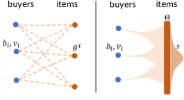
Figure 1: Budgets, values and supply.

• The budget $b_{i}$ of buyer $i$. Let $b=(b_{1},\dots,b_{n})$.

• The valuation for buyer $i$ is a function $v_{i}\in L^{1}_{+}$. Buyer $i$ has valuation $v_{i}(\theta)$ (per unit supply) of item $\theta\in\Theta$. Let $v:\Theta\to{\mathbb{R}^{n}}$, $v(\theta)=[v_{1}(\theta),\dots,v_{n}(\theta)]$. We assume ${\bar{v}}=\max_{i}\sup_{\theta}v_{i}(\theta)<\infty$. Also let $\nu_{i}=\int v_{i}s\mathop{}\!\mathrm{d}\theta$ be the monopolistic utility of buyer $i$, and ${\bar{\nu}}=\max_{i}\nu_{i}$.

• The supplies of items are given by a function $s\in L^{\infty}_{+}$, i.e., item $\theta\in\Theta$ has $s(\theta)$ units of supply. Without loss of generality, we assume a unit total supply $\int_{\Theta}s\mathop{}\!\mathrm{d}\theta=1$, which makes $s$ a probability measure. Let ${\mathbb{P}}$ denote the probability measure induced by $s$, i.e., ${\mathbb{P}}(A)=\int_{A}s{\mathop{}\!\mathrm{d}\theta}$ for a measurable set $A$. Given $g:\Theta\to{\mathbb{R}}$, we let ${\mathbb{E}}[g]=\int g(\theta)s(\theta)\mathop{}\!\mathrm{d}\theta$ and ${\operatorname{Var}}[g]={\mathbb{E}}[g^{2}]-({\mathbb{E}}[g])^{2}$. Given $t$ i.i.d. draws $\{\theta^{1},\dots,\theta^{t}\}$ from $s$, let $P_{t}g({\cdot})=\frac{1}{t}{\sum_{\tau=1}^{t}}g({\theta^{\tau}})$. Let ${v_{i}^{\tau}}=v_{i}({\theta^{\tau}})$.

Equilibria in both LFM and FPPE are characterized by a particular type of convex program known as an Eisenberg-Gale (EG) convex program. For statistical inference purposes, we will focus on the duals of these EG programs, which is a convex optimization problem over the space of pacing multipliers $\beta\in{\mathbb{R}^{n}_{+}}$ (these pacing multipliers turn out to represent the price-per-utility of buyers in equilibrium). In both cases, the dual EG objective separates into per-item convex terms

$$F(\theta,\beta)=f(\theta,\beta)-{\sum_{i=1}^{n}}b_{i}\log\beta_{i}\;,\;\;f(\theta,\beta)=\max_{i\in[n]}\beta_{i}v_{i}(\theta)\;.$$ (1)

and the population and sample EG objectives are

$$H(\beta)={\mathbb{E}}[F(\theta,\beta)]\;,\;\;H_{t}(\beta)=P_{t}F({\cdot},\beta)\;.$$ (2)

The reason we focus on the duals is that they can be cast as sample average approximations of the limit convex programs. This interpretation is not possible for the original primal EG programs.

2.1 Linear Fisher Markets (LFM)

The LFM model has two primary uses. Its original intent is as a model of competition, and how prices are determined in a competitive market. An additional, and practically important, use of LFM is as a tool for fair and efficient resource allocation (with the items being the resources). If every individual in a resource allocation problem is given one unit of faux currency, then the resulting LFM equilibrium allocation is known to be both Pareto efficient and satisfy the fairness desiderata of envy-freeness and proportionality (Nisan et al. 2007). This fair allocation approach is known as competitive equilibrium from equal incomes (CEEI) (Varian 1974).

We now describe the competitive equilibrium concept. Imagine there is a central policymaker that sets prices $p(\cdot)$ for the items $\Theta$. Upon observing the prices, buyer $i$ maximizes their utility subject to their budget. Their demand set is the set of bundles that are optimal under the prices:

$$D_{i}(p):=\argmax_{x_{i}\in L^{\infty}_{+}(\Theta)}\bigg{\{}\int v_{i}x_{i}s\mathop{}\!\mathrm{d}\theta:\int px_{i}s\mathop{}\!\mathrm{d}\theta\leq b_{i}\bigg{\}}\;.$$

Of course, due to the supply constraints, if prices are too low, there will be a supply shortage. On the other hand, if prices are too high, a surplus occurs. A competitive equilibrium is a set of prices and bundles such that all items are sold exactly at their supply (or have price zero). We call such an equilibrium the limit LFM equilibrium for the supply function $s$ (Gao and Kroer 2022).

Definition 2.1 (Limit LFM)

The limit equilibrium, denoted ${\mathsf{{LFM}}}(b,v,s,\Theta)$, is an allocation-price tuple $(x,p({\cdot}))$ such that the following holds.

1. (Supply feasibility and market clearance) $\sum_{i}x_{i}\leq 1$ and $\int p(1-\sum_{i}x_{i})s\mathop{}\!\mathrm{d}\theta=0$.

2. (Buyer optimality) $x_{i}\in D_{i}(p)$ all $i$.

Gao and Kroer (2022) show that an equilibrium of a limit LFM must exist, and that when the measure space $(\Theta,{\mathop{}\!\mathrm{d}\theta})$ is atomless, a pure equilibrium allocation must exist. Given an equilibrium $(x^{*},p^{*})$, let

$${u^{*}_{i}}=\int v_{i}s{x^{*}_{i}}\mathop{}\!\mathrm{d}\theta\;,\quad{\beta^{*}_{i}}=b_{i}/{u^{*}_{i}}\;,\quad{\mathsf{{NSW}}}^{*}={\sum_{i=1}^{n}}b_{i}\log({u^{*}_{i}})$$

be buyer $i$’ utility, her inverse bang-per-buck, and the (log) Nash social welfare of the whole market. The inverse bang-per-buck $\beta_{i}^{*}$ can also be seen as the price-per-utility of buyer $i$ in equilibrium. In a general LFM, the equilibrium allocation may not be unique, but the equilibrium quantities $p^{*},\beta^{*},u^{*}$ are unique. In order to facilitate statistical inference, we will impose certain differentiability condition, which turn out to imply uniqueness and purity of the equilibrium allocation $x^{*}$.

Next we introduce the finite LFM, which models the data we observe in a market. The finite LFM equilibrium is nothing but a limit LFM equilibrium where the item set $\Theta$ is the finite set of observed items $\gamma$. Let ${\gamma}=\{\theta^{1},\dots,\theta^{t}\}$ be $t$ i.i.d. samples from the supply distribution $s$, each with supply $\sigma\in{\mathbb{R}_{+}}$.

Definition 2.2 (Finite LFM, Eisenberg and Gale (1959), Eisenberg (1961))

The finite observed LFM, denoted ${\widehat{\mathsf{{LFM}}}}(b,v,\sigma,\gamma)$, is a allocation-price tuple $({x},p)\in{\mathbb{R}}^{t\times n}_{+}\times{\mathbb{R}^{n}_{+}}$ such that the following hold:

1. (Supply feasibility and market clearance) ${\sum_{i}}{x^{\tau}_{i}}\leq 1$ and $\sum_{\tau}{p^{\tau}}(1-{\sum_{i}}{x_{i}^{\tau}})=0$.

2. (Buyer optimality) $x_{i}\in D_{i}(p)=\argmax_{x_{i}}\{\sum_{\tau}{x_{i}^{\tau}}{v_{i}^{\tau}}:\sigma\sum_{\tau}{x_{i}^{\tau}}{p^{\tau}}\leq b_{i},{x_{i}^{\tau}}\geq 0\}$, the demand set given the prices.

Let $(x^{\gamma},{p^{\gamma}})\in{\widehat{\mathsf{{LFM}}}}(b,v,\sigma=1/t,\gamma)$ , where $x^{\gamma}=({x_{i}^{\tau}})_{i,\tau}$ and price ${p^{\gamma}}=[p^{1},\dots,p^{t}]$. Buyer $i$’s utility is $u^{\gamma}_{i}=\sigma{\sum_{\tau=1}^{t}}{v_{i}^{\tau}}{x^{\tau}_{i}}=\frac{1}{t}{\sum_{\tau=1}^{t}}{v_{i}^{\tau}}{x^{\tau}_{i}}$, and the inverse bang-per-buck is $\beta^{\gamma}_{i}=b_{i}/u^{\gamma}_{i}$. The (log) Nash social welfare is ${\mathsf{{NSW}}}^{\gamma}={\sum_{i}}b_{i}\log(u^{\gamma}_{i})$.

We now introduce several properties of LFM: natural bounds on $\beta$, fairness and efficiency as a resource allocation mechanism, scale-invariance, and the convex program characterization.

There exists natural bounds on $\beta^{*}$ in limit LFM. Recall $\nu_{i}=\int v_{i}s{\mathop{}\!\mathrm{d}\theta}$ is the expected value of buyer $i$. By Gao and Kroer (2022), we know that $b_{i}/\nu_{i}\leq{\beta^{*}_{i}}\leq(\sum_{i^{\prime}}b_{i^{\prime}})/(\min_{i^{\prime}}\nu_{i^{\prime}})$. We define

$$C_{\mathsf{{LFM}}}=\prod_{i=1}^{n}\bigg{[}\frac{b_{i}}{2\nu_{i}},\frac{2\sum_{i^{\prime}}b_{i^{\prime}}}{\min_{i^{\prime}}\nu_{i^{\prime}}}\bigg{]}\subset{\mathbb{R}^{n}_{+}}$$ (3)

to be the region whose interior $\beta^{*}$ must lie in.

A major use case for LFM is fair and efficient allocation of resources. Similar to the classical finite LFM, the infinite LFM enjoys fairness and efficiency properties (Gao and Kroer 2022). Let $x^{*}$ be an equilibrium allocation. First, this allocation is Pareto optimal, meaning there does not exist an $\tilde{x}\in(L_{+}^{\infty})^{n}$, ${\sum_{i}}\tilde{x}_{i}\leq 1$, such that $\int v_{i}\tilde{x}_{i}s{\mathop{}\!\mathrm{d}\theta}\geq\int v_{i}{x^{*}_{i}}s{\mathop{}\!\mathrm{d}\theta}$ for all $i$ and one of the inequalities is strict. The allocation $x^{*}$ is envy-free in a budget-weighted sense, meaning $\int v_{i}{x^{*}_{i}}s{\mathop{}\!\mathrm{d}\theta}/b_{i}\geq\int v_{j}x^{*}_{j}s{\mathop{}\!\mathrm{d}\theta}/b_{j}$ for all $i\neq j$. Finally, it is proportional: $\int v_{i}{x^{*}_{i}}s{\mathop{}\!\mathrm{d}\theta}\geq\int v_{i}s{\mathop{}\!\mathrm{d}\theta}\cdot(b_{i}/\sum_{i^{\prime}}b_{i^{\prime}})$, that is, each buyer gets at least the utility of its proportional share allocation.

LFM enjoys certain scale-invariance properties. First, buyers cannot change the equilibrium by scaling their value functions. Suppose $\alpha_{1},\dots,\alpha_{n}$ are positive scalars, and that $(x,p)$ are the equilibrium allocations and prices in ${\mathsf{{LFM}}}(b,v,s,\Theta)$. Then $(x,p)$ will also be the equilibrium quantities in ${\mathsf{{LFM}}}(b,(\alpha_{1}v_{1},\dots,\alpha_{n}v_{n}),s,\Theta)$. This is easily seen by the fact that valuation scaling does not change the demand function. Second, if all buyers’ budgets are scaled by the same factor, or the supply is scaled by the same factor, the equilibrium does not change. That is, if $\alpha_{1},\alpha_{2}$ are two positive scalars, and $(x,p)={\mathsf{{LFM}}}(b,v,s,\Theta)$, then $(x,(\alpha_{1}/\alpha_{2})p)={\mathsf{{LFM}}}(\alpha_{1}b,v,\alpha_{2}s,\Theta)$. These scale-invariances hold for finite LFM as well . Based on the invariance, we impose the normalization that ${\sum_{i=1}^{n}}b_{i}=1$ and that all buyers’ expected values are 1, i.e., $\int v_{i}(\theta)s(\theta)\mathop{}\!\mathrm{d}\theta=1$. Then in the limit LMF, the budge-supply ratio is ${\sum_{i=1}^{n}}b_{i}/\int s\mathop{}\!\mathrm{d}\theta=1$. With the normalization, we have $C_{\mathsf{{LFM}}}=\prod_{i=1}^{n}[b_{i}/2,2]$. In order for the budget-to-supply ratio to match in the sampled finite LFM and the limit LFM, we use supplies of $1/t$ for each item in the finite LFM. Thus we study finite LFM of the form ${\widehat{\mathsf{{LFM}}}}(b,v,1/t,\gamma)$.

It is well-known (Eisenberg and Gale 1959, Cole et al. 2017, Gao and Kroer 2022) that the equilibrium inverse bang-per-buck in a limit (resp. finite) LFM uniquely solves the population (resp. sample) dual EG program

$$\beta^{*}=\argmin_{\beta\in{\mathbb{R}^{n}_{+}}}H(\beta)\;,\;\beta^{\gamma}=\argmin_{\beta\in{\mathbb{R}^{n}_{+}}}H_{t}(\beta)\;.$$ (4)

2.2 First-Price Pacing Equilibrium (FPPE)

The FPPE setting (Conitzer et al. 2022a) models an economy that typically occurs on internet advertising platforms: the buyers (advertisers in the internet advertising setting) are subject to budget constraints, and must participate in a set of first-price auctions, each of which sells a single item. Each buyer is assigned a pacing multiplier $\beta_{i}\in[0,1]$ by the platform to scale down their bids in the auctions, and submits bids of the form $\beta_{i}v_{i}(\theta)$ for each item $\theta$. From the platform’s perspective, the goal of choosing $\beta_{i}$ is to ensure there is no unnecessary pacing, i.e., buyers spend their budget exactly, or they spend less than their budget but they do not scale down their bids. In the FPPE model, all auctions occur simultaneously, and thus the buyers choose a single $\beta_{i}$ that determines their bid in all auctions. The utility of a buyer in FPPE is quasilinear: it is the sum of their value received from items plus their leftover budget (this is equivalent for decision-making purposes to the utility being the value received from items minus the payments).

Definition 2.3 (Limit FPPE, Gao and Kroer (2022))

A limit FPPE, denoted ${\textsf{{FPPE}}}(b,v,s,\Theta)$, is the unique tuple $(\beta,p({\cdot}))\in[0,1]^{n}\times L^{1}_{+}(\Theta)$ such that there exist $x_{i}:\Theta\to[0,1]$, $i\in[n]$ satisfying

1. (First-price) Prices are determined by first-price auctions: for all items $\theta\in\Theta$, $p(\theta)=\max_{i}\beta_{i}v_{i}(\theta)$. Only the highest bidders win: for all $i$ and $\theta$, $x_{i}(\theta)>0$ implies $\beta_{i}{v_{i}(\theta)}=\max_{k}\beta_{k}v_{k}(\theta)$

2. (Feasibility, market clearing) Let ${\small\textsf{{pay}}}_{i}=\int x_{i}(\theta)p(\theta)s(\theta)\mathop{}\!\mathrm{d}\theta$ be the expenditure of buyer $i$. Buyers satisfy budgets: for all $i$, ${\small\textsf{{pay}}}_{i}\leq b_{i}$. There is no overselling: for all $\theta$, ${\sum_{i=1}^{n}}x_{i}(\theta)\leq 1$. All items are fully allocated: for all $\theta$, $p(\theta)>0$ implies ${\sum_{i=1}^{n}}x_{i}(\theta)=1$.

3. (No unnecessary pacing) For all $i$, ${\small\textsf{{pay}}}_{i}<b_{i}$ implies $\beta_{i}=1$.

FPPE is a hindsight and static solution concept for internet ad auctions. Suppose the platform knows all the items that are going to show up on a platform. FPPE describes how the platform could configure the $\beta_{i}$’s in a way that ensures that all buyers satisfy their budgets, while maintaining their expressed valuation ratios between items. In practice, the $\beta_{i}$’s are learned by an online algorithm that is run by the platform (Balseiro and Gur 2019, Conitzer et al. 2022a). FPPE has many nice properties, such as the fact that it is a competitive equilibrium, it is revenue-maximizing, revenue-monotone, shill-proof, has a unique set of prices, and so on (Conitzer et al. 2022a). We refer readers to Conitzer et al. (2022a), Kroer and Stier-Moses (2022) for more context about the use of FPPE in internet ad auctions.

Gao and Kroer (2022) show that a limit FPPE always exists and is unique, and when the item space is atomless, a pure allocation exists. Let $\beta^{*}$ and $p^{*}$ be the unique FPPE equilibrium multipliers and prices. Revenue in the limit FPPE is

$${\mathsf{{REV}}}^{*}=\int p^{*}(\theta)s(\theta)\mathop{}\!\mathrm{d}\theta\;.$$ (5)

It is also easy to see that ${\mathsf{{REV}}}^{*}={\sum_{i}}{\small\textsf{{pay}}}_{i}$. Although the equilibrium allocation $x^{*}$ may not be unique in general, for statistical inference we will impose certain differentiability assumption which imply uniqueness of $x^{*}$. When $x^{*}$ is unique, we let ${\delta^{*}_{i}}=b_{i}-{\small\textsf{{pay}}}_{i}$ be the leftover budget.

In an FPPE, based on the pacing multiplier and the budget expenditure, we can categorize buyers in terms of how they satisfy the no unnecessary pacing condition. As we will see later, the statistical behavior of pacing multipliers varies by category.

• Paced buyers (${\beta^{*}_{i}}<1$). We use $I^{c}=\{i:{\beta^{*}_{i}}<1\}$ to denote them. Due to the budget constraints, they are not able to bid their value in the auctions at equilibrium, and by the no unnecessary pacing condition in Def. 2.3, their budgets are fully exhausted, i.e. ${\delta^{*}_{i}}=0$.

• Unpaced buyers (${\beta^{*}_{i}}=1$). We use $I=\{i:{\beta^{*}_{i}}=1\}$ to denote them. They can be further divided according to their budget expenditure.

  • Buyers who have leftover budgets (${\beta^{*}_{i}}=1,0<{\delta^{*}_{i}}\leq b_{i}$), denoted $I_{+}$. Note this category also includes buyers who dot not win any items (${\beta^{*}_{i}}=1,{\delta^{*}_{i}}=b_{i}$).

  • Degenerate buyers (${\beta^{*}_{i}}=1,{\delta^{*}_{i}}=0$), denoted $I_{0}$. They are the edge-cases in the FPPE model. If these buyers were given more budgets, they would become $I_{+}$-type buyers at equilibrium. For the FPPE statistical theory developed in this paper, we assume absence of such buyers (Section 5.2). In follow-up work to the conference version of the present paper, Liao and Kroer (2024) give some results for the case where degenerate buyers exist.

We let ${\gamma}=\{\theta^{1},\dots,\theta^{t}\}$ be $t$ i.i.d. draws from $s$, each with supply $\sigma=1/t$. They represent the items observed in an auction market. The definition of a finite FPPE is parallel to that of a limit FPPE, except that we change the supply function to be a discrete distribution supported on $\gamma$.

Definition 2.4 (Finite FPPE, Conitzer et al. (2022a))

The finite observed FPPE, ${\widehat{\textsf{{FPPE}}}}(b,v,\sigma,\gamma)$, is the unique tuple $(\beta,p)\in[0,1]^{n}\times{\mathbb{R}}^{t}_{+}$ such that there exists $x_{i}^{\tau}\in[0,1]$ satisfying:

1. (First-price) For all $\tau$, ${p^{\tau}}=\max_{i}\beta_{i}{v_{i}^{\tau}}$. For all $i$ and $\tau$, ${x_{i}^{\tau}}>0$ implies $\beta_{i}{v_{i}^{\tau}}=\max_{k}\beta_{k}v_{k}^{\tau}$.

2. (Supply and budget feasible) For all $i$, $\sigma\sum_{\tau}{x_{i}^{\tau}}{p^{\tau}}\leq b_{i}$. For all $\tau$, ${\sum_{i}}{x_{i}^{\tau}}\leq 1$.

3. (Market clearing) For all $\tau$, ${p^{\tau}}>0$ implies ${\sum_{i}}{x_{i}^{\tau}}=1$.

4. (No unnecessary pacing) For all $i$, $\sigma\sum_{\tau}{x_{i}^{\tau}}{p^{\tau}}<b_{i}$ implies $\beta_{i}=1$.

Let $(\beta^{\gamma},{p^{\gamma}})={\widehat{\textsf{{FPPE}}}}(b,v,\sigma=1/t,\gamma)$. Given the equilibrium price ${p^{\gamma}}=[p^{1},\dots,p^{t}]^{\top}$, the revenue in a finite FPPE is ${\mathsf{{REV}}}^{\gamma}=\sigma{\sum_{\tau=1}^{t}}{p^{\tau}}=\frac{1}{t}{\sum_{\tau=1}^{t}}{p^{\tau}}$.

FPPE has some of the same scale-invariance properties as LFM. In particular, scaling the budget and supply at the same time does not change the market equilibrium. That is, given a positive scalar $\alpha$, if $(\beta,p)$ are the equilibrium pacing multiplier and prices in the market ${\textsf{{FPPE}}}(b,v,s,\Theta)$, then $(\beta,p)$ are the equilibrium quantities in the market ${\textsf{{FPPE}}}(\alpha b,v,\alpha s,\Theta)$. The same scale-invariance holds for the finite FPPE, i.e., if $(\beta,p)={\widehat{\textsf{{FPPE}}}}(b,v,\sigma,\gamma)$, then $(\beta,p)={\widehat{\textsf{{FPPE}}}}(\alpha b,v,\alpha\sigma,\gamma)$. Given the invariance, we can see that in order for the budget-supply ratio to match the limit market ${\textsf{{FPPE}}}(b,v,s,\Theta)$, the finite market should be configured as either ${\widehat{\textsf{{FPPE}}}}(tb,v,1,\gamma)$ or ${\widehat{\textsf{{FPPE}}}}(b,v,1/t,\gamma)$. We will study the latter, and simply refer to it as the finite FPPE. Unlike LFM, FPPE does not enjoy invariance to valuation scaling, because buyers have a pacing multiplier of at most one in FPPE.

It is well-known (Cole et al. 2017, Conitzer et al. 2022a, Gao and Kroer 2022) that $\beta$ in a limit (resp. finite) FPPE uniquely solves the population (resp. sample) dual EG program

$$\beta^{*}=\argmin_{\beta\in(0,1]^{n}}H(\beta)\;,\;\beta^{\gamma}=\argmin_{\beta\in(0,1]^{n}}H_{t}(\beta)\;,$$ (6)

where the objectives $H$ and $H_{t}$ are the same as in Eq. 4. The difference between the LFM and FPPE convex programs is that for FPPE we impose the constraint $(0,1]^{n}$.

The EG program and certain quantities of the FPPE are related as follows.

Lemma 2.5

Suppose $H$ is twice continuously differentiable at $\beta^{*}$, the equilibrium pacing multiplier. Then $\nabla H(\beta^{*})=-{\delta^{*}}$, and $\nabla^{2}H(\beta^{*})\beta^{*}=[b_{1}/\beta^{*}_{1},\dots,b_{n}/\beta^{*}_{n}]^{\top}$.

Proof sketch The first equality follows from the fact that leftover budgets are the Lagrange multipliers corresponding to the constraint $\beta\leq 1\in{\mathbb{R}^{n}}$. The second equality follows from the first-order homogeneity of $f(\theta,\beta)=\max_{i}\beta_{i}{v_{i}(\theta)}$ in Eq. 1. See Section 12 for details.

3 Differentiability of EG Objective

This section is dedicated to describing the differentiability properties of the EG objective $H$ in Eq. 2. The second part of $H$ is clearly a nice function, and so we focus on its first part ${\bar{f}}(\beta)={\mathbb{E}}[f(\theta,\beta)]$. Differentiability of the EG objective is important because the following assumption is needed when deriving the asymptotic distribution of LFM and FPPE.

[SMO] Let $\beta^{*}$ denote the equilibrium inverse bang-per-buck in LFM, or the equilibrium pacing multiplier in FPPE. Assume the map $\beta\mapsto{\bar{f}}(\beta)={\mathbb{E}}_{s}[\max_{i}\beta_{i}{v_{i}(\theta)}]$ is $C^{2}$ in a neighborhood of $\beta^{*}$. We let ${\mathcal{H}}=\nabla^{2}H(\beta^{*})$.

We start with the differential structure of $f(\theta,\beta)=\max_{i}\beta_{i}{v_{i}(\theta)}$. The function $f(\theta,\beta)$ is a convex function of $\beta$ and its subdifferential $\partial_{\beta}f(\theta,\beta)$ is the convex hull of $\{v_{i}e_{i}\in{\mathbb{R}^{n}_{+}}:\text{index $i$ such that $\beta_{i}{v_{i}(\theta)}=\max_{k}\beta_{k}v_{k}(\theta)$}\}$, with $e_{i}$ being the base vector in ${\mathbb{R}^{n}}$. When $\max_{i}\beta_{i}v_{i}(\theta)$ is attained by a unique $i^{*}$, the function $f$ is differentiable. In that case, the $i$-th entry of $\nabla_{\beta}f(\theta,\beta)$ is $v_{i}(\theta)$ for $i=i^{*}$ and zero otherwise.

3.1 First-order Differentiability

We introduce notation for characterizing first-order differentiability of ${\bar{f}}(\beta)={\mathbb{E}}_{s}[f(\theta,\beta)]$. Define the gap between the highest and the second-highest bid under pacing multiplier $\beta$ by

$${\mathsf{{bidgap}}}(\beta,\theta)=\max\{\beta_{i}{v_{i}(\theta)}\}-\operatorname{secondmax}\{\beta_{i}{v_{i}(\theta)}\}\;,$$ (7)

here $\operatorname{secondmax}$ is the second-highest entry; e.g., $\operatornamewithlimits{secondmax}([1,1,2])=1$. When there is a tie for an item $\theta$, we have ${\mathsf{{bidgap}}}(\beta,\theta)=0$. When there is no tie for an item $\theta$, the gap ${\mathsf{{bidgap}}}(\beta,\theta)$ is strictly positive. The gap function characterizes smoothness of $f$: $f(\cdot,\theta)$ is differentiable at $\beta$ iff ${\mathsf{{bidgap}}}(\beta,\theta)$ is strictly positive.

Theorem 3.1 (First-order differentiability)

The following are equivalent. (i) The dual objective $H$ is differentiable at a point $\beta$. (ii) The function $\theta\mapsto{\mathsf{{bidgap}}}(\beta,\theta)$ is strictly positive $s$-almost surely:

$${\mathbb{P}}(\theta:{\mathsf{{bidgap}}}(\beta,\theta)>0)=1\;.$$ (8)

(iii) The set of items that incur ties under pacing profile $\beta$ is $s$-measure zero: ${\mathbb{P}}(\theta\in\Theta:\beta_{i}{v_{i}(\theta)}=\beta_{k}v_{k}(\theta)\text{ for some $i\neq k$})=0$.

When one and thus all of the above conditions hold for some $\beta$, the gradient $\nabla_{\beta}f(\theta,\beta)$ is well-defined for $s$-almost every $\theta$, and $\nabla{\bar{f}}(\beta)={\mathbb{E}}[\nabla f(\theta,\beta)]$. Proof and further technical remarks given in Section 8.2.

3.2 Second-order Differentiability

Given the neat characterization of differentiability of the dual objective via the gap function ${\mathsf{{bidgap}}}(\beta,\theta)$, it is natural to explore higher-order smoothness, which is needed for some of our asymptotic normality results. Example 8.3 in the appendix is one where Eq. 8 holds at a point, say $\beta$, and ${\bar{f}}$ is differentiable in a neighborhood of $\beta$, and yet ${\bar{f}}$ is not twice differentiable at $\beta$. We now provide three sufficient conditions that imply twice differentiability of objective $H$.

Theorem 3.2 (Second-order differentiability, informal)

If any of the following conditions hold, then ${\bar{f}}$ and thus $H$ are $C^{2}$ at a point $\beta$. (i) A stronger form of Eq. 8 holds: ${\mathbb{E}}[{\mathsf{{bidgap}}}(\beta,\theta)^{-1}]<\infty$. (ii) The angular component of the random vector $v=(v_{1},\dots,v_{n}):\Theta\to{\mathbb{R}^{n}_{+}}$ is smoothly distributed. (iii) $\Theta=[0,1]$, $s$ is the Lebesgue measure, the valuations $v_{i}(\cdot)$’s are linear functions, and $\beta$ is the equilibrium inverse bang-per-buck in LFM. See Appendix 8 for formal statements.

We show in Appendix 8.3 that when $H$ is twice differentiable, the Hessian matrix of $H$ has a closed-form expression.

4 Statistical Results for Linear Fisher Markets

We now turn to investigating the statistical convergence properties of finite LFMs to the limit LFM. Suppose we sample an LFM (${\widehat{\mathsf{{LFM}}}}(b,v,1/t,\gamma)$), where $\gamma$ consists of $t$ i.i.d. samples from $s$. We will study how such finite LFMs are distributed around the limit LFM (${\mathsf{{LFM}}}(b,v,s,\Theta)$) as $t$ grows. In LFM we focus on convergence of the following quantities: individual utilities, (log) Nash social welfare (NSW), and the pacing multiplier vector $\beta$ (which characterizes the equilibrium, as shown in Eq. 4). Section 4.1 presents strong consistency and convergence rate results. Section 4.2 presents asymptotic distributions for the quantities of interest, and a local minimax theory based on Le Cam et al. (2000), showing that the finite LFM provides an optimal estimate for the limit LFM in a local asymptotic sense. Section 4.3 discusses estimation of asymptotic variance of NSW.

4.1 Basic Convergence Properties

In this section we show that we can treat observed quantities in the finite LFM as consistent estimators of their counterparts in the limit LFM. Below we state the consistency results; the formal versions can be found in Section 9.1. We say an estimator sequence $\{\hat{a}_{t}\}$ is strongly consistent for $a$ if ${\mathbb{P}}(\lim_{t\to\infty}\hat{a}_{t}=a)=1$.

Theorem 4.1 (Strong Consistency)

The NSW, pacing multiplier vector, and utility vectors in the finite LFM are strongly consistent estimators of their counterparts in the limit LFM.

Next, we refine the consistency results and provide finite sample guarantees. We start by focusing on Nash social welfare and the set of approximate market equilibria. The convergence of utilities and pacing multipliers will then be derived from the latter result.

Theorem 4.2

For any failure probability $0<\eta<1$, let $t\geq 2{{\bar{v}^{2}}{\log(4n/\eta)}}$. Then with probability greater than $1-\eta$, we have $|{\mathsf{{NSW}}}^{\gamma}-{\mathsf{{NSW}}}^{*}|\leq O(1){{\bar{v}}\big{(}\sqrt{n\log((n+{\bar{v}})t)}+\sqrt{\log(1/\eta)}\big{)}}{t^{-1/2}},$ where $O(1)$ hides only constants. Proof in Appendix 11.2.

Theorem 4.2 establishes a convergence rate $|{\mathsf{{NSW}}}^{\gamma}-{\mathsf{{NSW}}}^{*}|=\tilde{O}_{p}({\bar{v}}\sqrt{n}t^{-1/2})$. The proof proceeds by first establishing a pointwise concentration inequality and then applies a discretization argument.

To state the result for the pacing multipliers $\beta$, we define approximate market equilibria (which we define in terms of approximately optimal pacing multiplier vectors $\beta$). Let

$${\mathcal{B}}^{\gamma}(\epsilon)=\{\beta\in{\mathbb{R}^{n}_{++}}:H_{t}(\beta)\leq\inf_{\beta}H_{t}(\beta)+\epsilon\},\;{\mathcal{B}}^{*}(\epsilon)=\{\beta\in{\mathbb{R}^{n}_{++}}:H(\beta)\leq\inf_{\beta}H(\beta)+\epsilon\}\;.$$ (9)

be the sets of $\epsilon$-approximate solutions to the sample and the population EG programs, respectively. The next theorem shows that the set of $\epsilon/2$-approximate solutions to the sample EG program is contained in the set of $\epsilon$-approximate solutions to the population EG program with high probability.

Theorem 4.3 (Convergence of Approximate Market Equilibrium)

Let ${\epsilon}>0$ be a tolerance parameter and $\alpha\in(0,1)$ be a failure probability. Then for any $0\leq\delta\leq{\epsilon}/2$, to ensure ${\mathbb{P}}\big{(}C_{\mathsf{{LFM}}}\cap{\mathcal{B}^{\gamma}}(\delta)\subset C_{\mathsf{{LFM}}}\cap{\mathcal{B}^{*}}(\epsilon)\big{)}\geq 1-2\alpha$ it suffices to set

$$t\geq O(1){\bar{v}^{2}}\min\bigg{\{}\frac{1}{\underaccent{\bar}{b}\epsilon},\frac{1}{\epsilon^{2}}\bigg{\}}\bigg{(}n\log\Big{(}\tfrac{16(2n+{\bar{v}})}{{\epsilon}-\delta}\Big{)}+\log\tfrac{1}{\alpha}\bigg{)}\;,$$ (10)

where the set $C_{\mathsf{{LFM}}}$, defined in Eq. 3, is the natural region in which $\beta^{*}$ must lie, and $O(1)$ hides absolute constants. Proof in Appendix 11.3.

By construction of $C_{\mathsf{{LFM}}}$ we know $\beta^{*}\in C_{\mathsf{{LFM}}}$ holds, and so $C_{\mathsf{{LFM}}}\cap{\mathcal{B}^{*}}(\epsilon)$ is not empty. In the appendix, Lemma 10.1 shows that for $t$ sufficiently large, $\beta^{\gamma}\in C_{\mathsf{{LFM}}}$ with high probability, in which case the set $C_{\mathsf{{LFM}}}\cap{\mathcal{B}^{\gamma}}(\delta)$ is not empty. By simply taking $\delta=0$ in Theorem 4.3 we obtain the corollary below.

Corollary 4.4

Let $t$ satisfy Eq. 10. Then with probability $\geq 1-2\alpha$ it holds $H(\beta^{\gamma})\leq H(\beta^{*})+\epsilon$.

More importantly, it establishes the fast statistical rate $H(\beta^{\gamma})-H(\beta^{*})=\tilde{O}_{p}(t^{-1})$ for $t$ sufficiently large, where we use $\tilde{O}_{p}$ to ignore logarithmic factors. In words: the limit LFM objective value of the finite LFM solution $\beta^{\gamma}$ converges to the optimal limit LFM objective value with a rate $1/t$.

By the strong convexity of the dual objective, the containment result can be translated to high-probability convergence of the pacing multipliers and the utility vector.

Corollary 4.5

Let $t$ satisfy Eq. 10. Then with probability at least $1-2\alpha$ we have $\|\beta^{\gamma}-\beta^{*}\|_{2}\leq\sqrt{\frac{8\epsilon}{\underaccent{\bar}{b}}}$ and $\|u^{\gamma}-u^{*}\|_{2}\leq\frac{4}{\underaccent{\bar}{b}}\sqrt{8\epsilon/\underaccent{\bar}{b}}$.

We compare the above corollary with Theorem 9 from Gao and Kroer (2022) which establishes the convergence rate of the stochastic approximation estimator based on the dual averaging algorithm (Xiao 2010). In particular, they show that the average of the iterates, denoted $\beta_{\mathrm{DA}}$, enjoys a convergence rate of $\|\beta_{\mathrm{DA}}-\beta^{*}\|_{2}^{2}=\tilde{O}_{p}\big{(}\frac{{\bar{v}}^{2}}{\underaccent{\bar}{b}^{2}}\frac{1}{t}\big{)}$, where $t$ is the number of sampled items. The rate achieved in Corollary 4.5 is $\|\beta^{\gamma}-\beta^{*}\|_{2}^{2}=\tilde{O}_{p}\big{(}\frac{n{\bar{v}^{2}}}{\underaccent{\bar}{b}^{2}}\frac{1}{t}\big{)}$. We see that our rate is worse off by a factor of $n$. We conjecture that it can be removed by using the more involved localization arguments (Bartlett et al. 2005). And yet our estimates are produced by the strategic behavior of the agents without any extra computation at all. Moreover, in the computation of the dual averaging estimator the knowledge of the values $v_{i}(\theta)$ is required, while again $\beta^{\gamma}$ can be just observed naturally.

4.2 Asymptotics of Linear Fisher Market

In this section we derive asymptotic normality results for Nash social welfare, utilities and pacing multipliers. As we will see, a central limit theorem for Nash social welfare holds under basically no additional assumptions. However, the CLTs of pacing multipliers and utilities will require twice continuous differentiability of the population dual objective $H$ at optimality, with a nonsingular Hessian matrix. We present CLT results under such a premise; Theorem 3.2 gave three quite general settings under which these conditions hold.

Theorem 4.6 (Asymptotic Normality of Nash Social Welfare)

It holds that

$$\sqrt{t}({\mathsf{{NSW}}}^{\gamma}-{\mathsf{{NSW}}}^{*}){\,\overset{{\,d\,\,}}{\rightarrow}\,}{\mathcal{N}}(0,\sigma^{2}_{{\mathsf{{NSW}}}})\;,$$ (11)

where $\sigma^{2}_{{\mathsf{{NSW}}}}={\operatorname{Var}}(p^{*})=\int(p^{*})^{2}s{\mathop{}\!\mathrm{d}\theta}-(\int p^{*}s{\mathop{}\!\mathrm{d}\theta})^{2}$. Proof in Appendix 11.4.

As stated previously, our asymptotic results for $\beta$ and $u$ require that $H$ is twice-continuously differentiable at $\beta^{*}$. When this differentiability holds, by Theorem 3.1, the set of items that incur ties is $s$-measure zero, and thus the equilibrium allocation $x^{*}$ in the limit LFM is unique and must be pure. Now we define a map ${\mu^{*}}:\Theta\to{\mathbb{R}^{n}_{+}}$, which represents the utility all buyers obtain from the item $\theta$ at equilibrium. Formally,

$${\mu^{*}}(\theta)=[x^{*}_{1}(\theta)v_{1}(\theta),\dots,x^{*}_{n}(\theta)v_{n}(\theta)]^{\top}.$$ (12)

Since $x^{*}$ is pure, only one entry of ${\mu^{*}}(\theta)$ is nonzero. Clearly $\int{\mu^{*}}s\mathop{}\!\mathrm{d}\theta=[u^{*}_{1},\dots,u^{*}_{n}]^{\top}$.

Theorem 4.7 (Asymptotic Normality of Pacing Multipliers and Utilities)

Let Section 3 hold with non-singular Hessian matrix ${\mathcal{H}}=\nabla^{2}H(\beta^{*})$. Then

$$\sqrt{t}(\beta^{\gamma}-\beta^{*}){\,\overset{{\,d\,\,}}{\rightarrow}\,}\allowbreak{\mathcal{N}}\big{(}0,\Sigma_{\beta}\big{)},\quad\sqrt{t}(u^{\gamma}-u^{*}){\,\overset{{\,d\,\,}}{\rightarrow}\,}\allowbreak{\mathcal{N}}\big{(}0,\Sigma_{u}\big{)},$$ (13)

where $\Sigma_{\beta}={\mathcal{H}}^{-1}\allowbreak{\operatorname{Cov}}({\mu^{*}}){\mathcal{H}}^{-1}$ and $\Sigma_{u}={\operatorname*{diag}}(-b_{i}/({\beta^{*}_{i}})^{2})\allowbreak{\mathcal{H}}^{-1}\allowbreak{\operatorname{Cov}}({\mu^{*}})\allowbreak{\mathcal{H}}^{-1}\allowbreak{\operatorname*{diag}}(-b_{i}/({\beta^{*}_{i}})^{2}).$ Proof in Appendix 11.4.

Theorem 4.6 can also be derived from Theorem 4.7 using the delta method, since ${\mathsf{{NSW}}}^{*}={\sum_{i=1}^{n}}b_{i}\log({u^{*}_{i}})={\sum_{i}}b_{i}\log(b_{i}/{\beta^{*}_{i}})$ is a smooth function of $\beta^{*}$.

We will show that the asymptotic variances in Theorem 4.7 are the best achievable, in an asymptotic local minimax sense. To make this precise, we need to introduce “supply neighborhoods” obtained through perturbing the original supply $s$.

4.2.1 Perturbed Supply

First we introduce notation to parametrize neighborhoods of the supply $s$. Let $g\in G_{d}=\{g:\Theta\to{\mathbb{R}}^{d}:{\mathbb{E}}[g]=0,{\mathbb{E}}[\|g\|^{2}]<\infty\}$ be a direction along which we wish to perturb the supply $s$. Given a vector $\alpha\in{\mathbb{R}}^{d}$ signifying the magnitude of perturbation, we want to scale the original supply of item $\theta$ by $\exp(\alpha^{\top}g(\theta))$ and then obtain a perturbed supply distribution by appropriate normalization. To do this we define the perturbed supply by

$$s_{\alpha,g}(\theta)=C^{-1}[{1+\alpha^{\top}g(\theta)}]s(\theta)$$ (14)

with a normalizing constant $C=1+\int\alpha^{\top}g(\theta)s(\theta)\mathop{}\!\mathrm{d}\theta$. As $\alpha\to 0$, the perturbed supply $s_{\alpha,g}$ effectively approximates $s_{\alpha,g}(\theta)\propto\exp(\alpha^{\top}g(\theta))s(\theta).$

We let $\beta^{*}_{\alpha,g}$, $u^{*}_{\alpha,g}$ and ${\mathsf{{NSW}}}^{*}_{\alpha,g}$ be the limit inverse bang-per-buck, price and revenue in ${\mathsf{{LFM}}}(b,v,s_{\alpha,g},\Theta)$. Clearly $\beta^{*}=\beta^{*}_{0,g}$ for any $g$ and similarly for $u^{*}_{0,g}$ and ${\mathsf{{NSW}}}_{0,g}$.

4.2.2 Asymptotic Local Minimax Optimality

Given the asymptotic normality of observed LFM, it is desirable to understand the best possible statistical procedure for estimating the limit LFM. One way to discuss the optimality is to measure the difficulty of estimating the limit LFM when the supply distribution varies over small neighborhoods of the true supply $s$, asymptotically. When an estimator achieves the best worst-case risk over these small neighborhoods, we say it is asymptotically locally minimax optimal. For general references, see Vaart and Wellner (1996), Le Cam et al. (2000). More recently Duchi and Ruan (2021, Sec. 3.2) develop asymptotic local minimax theory for constrained convex optimization, and we rely on their results.

Let $L:{\mathbb{R}^{n}}\to{\mathbb{R}}$ be any symmetric quasi-convex loss . In asymptotic local minimax theory we are interested in the local asymptotic risk: given a sequence of estimators $\{\hat{\beta}_{t}:\Theta^{t}\to{\mathbb{R}^{n}}\}_{t}$,

$${\mathsf{{LAR}}}_{\beta}(\{\hat{\beta}_{t}\}_{t})={\sup_{g\in G_{d},d\in\mathbb{N}}\lim_{c\to\infty}\liminf_{t\to\infty}\sup_{\|\alpha\|_{2}\leq\frac{c}{\sqrt{t}}}{\mathbb{E}}_{s_{\alpha,g}^{\otimes t}}[L(\sqrt{t}(\hat{\beta}_{t}-\beta^{*}_{\alpha,g}))]}\;.$$

If we ignore the limits and consider a fixed $t$, then ${\mathsf{{LAR}}}_{\beta}$ roughly measures the worst-case risk for the estimators $\{\hat{\beta}_{t}\}$. Note that $\alpha$ is a $d$-vector, and thus the shrinking norm-balls depend on $d$, and the expectation is taken w.r.t. the $t$-fold product of the perturbed supply.

Similarly, define the risk for utility $u$ (resp. Nash social welfare ${\mathsf{{NSW}}}$) given an estimator sequence $\{\hat{u}_{t}\}$ (resp. $\{\widehat{\mathsf{{NSW}}}_{t}\}$):

$${\mathsf{{LAR}}}_{u}(\{\hat{u}_{t}\}_{t})={\sup_{g\in G_{d},d\in\mathbb{N}}\lim_{c\to\infty}\liminf_{t\to\infty}\sup_{\|\alpha\|_{2}\leq\frac{c}{\sqrt{t}}}{\mathbb{E}}_{s_{\alpha,g}^{\otimes t}}[L(\sqrt{t}(\hat{u}_{t}-u^{*}_{\alpha,g}))]}\;,$$

$${\mathsf{{LAR}}}_{\mathsf{{NSW}}}(\{\widehat{\mathsf{{NSW}}}_{t}\}_{t})={\sup_{g\in G_{d},d\in\mathbb{N}}\lim_{c\to\infty}\liminf_{t\to\infty}\sup_{\|\alpha\|_{2}\leq\frac{c}{\sqrt{t}}}{\mathbb{E}}_{s_{\alpha,g}^{\otimes t}}[L(\sqrt{t}(\widehat{\mathsf{{NSW}}}_{t}-{\mathsf{{NSW}}}^{*}_{\alpha,g}))]}\;.$$

Theorem 4.8

Let Section 3 hold. Then

$$\inf_{\hat{\beta}_{t}}{\mathsf{{LAR}}}_{\beta}(\{\hat{\beta}_{t}\})\geq{\mathbb{E}}[L({\mathcal{N}}(0,\Sigma_{\beta}))]\;,$$

$$\inf_{\hat{u}_{t}}{\mathsf{{LAR}}}_{u}(\{\hat{u}_{t}\})\geq{\mathbb{E}}[L({\mathcal{N}}(0,\Sigma_{u}))]\;,$$

$$\inf_{\widehat{\mathsf{{NSW}}}_{t}}{\mathsf{{LAR}}}_{\mathsf{{NSW}}}(\{\widehat{\mathsf{{NSW}}}_{t}\})\geq{\mathbb{E}}[L({\mathcal{N}}(0,\sigma^{2}_{\mathsf{{NSW}}}))]\;,$$

where $\sigma^{2}_{\mathsf{{NSW}}}$ is defined in Theorem 4.6, and $\Sigma_{\beta},\Sigma_{u}$ in Theorem 4.7. Proof in Section 11.5

4.3 Variance Estimation and Inference

In this section we show how to construct confidence intervals for Nash social welfare. We will show how to construct confidence intervals for pacing multipliers and utilities in the FPPE section. The procedure is similar for LFM, and thus we omit it here.

First, regarding inference, it is interesting to note that the observed NSW (${\mathsf{{NSW}}}^{\gamma}$) is a negatively-biased estimate of the limit NSW (${\mathsf{{NSW}}}^{*}$), i.e., ${\mathbb{E}}[{\mathsf{{NSW}}}^{\gamma}]-{\mathsf{{NSW}}}^{*}\leq 0$. Moreover, it can be shown that, when the items are i.i.d. ${\mathbb{E}}[\min H_{t}]\leq{\mathbb{E}}[\min H_{t+1}]$ by a simple argument from Proposition 16 from Shapiro (2003). Monotonicity tells us that increasing the market size produces, on average, less biased estimates of the limit NSW.

To construct confidence intervals for Nash social welfare, one needs to estimate the asymptotic variance. Let ${p^{\tau}}$ be the price of item ${\theta^{\tau}}$ in the finite market, and $\bar{p}=\frac{1}{t}{\sum_{\tau=1}^{t}}{p^{\tau}}$. The variance estimator is then

$$\hat{\sigma}_{{\mathsf{{NSW}}}}^{2}=\frac{1}{t}{\sum_{\tau=1}^{t}}\big{(}{p^{\tau}}-\bar{p}\big{)}^{2}\;.$$ (15)

We emphasize that in the computation of the variance estimator $\hat{\sigma}_{{\mathsf{{NSW}}}}^{2}$ one does not need knowledge of the valuations $\{{v_{i}(\theta^{\tau})}\}_{i,\tau}$. All that is needed is the equilibrium prices ${p^{\gamma}}=(p^{1},\dots,p^{t})$ for the items. Given the variance estimator, we construct the confidence interval $\big{[}{\mathsf{{NSW}}}^{\gamma}\pm z_{\alpha/2}\frac{\hat{\sigma}_{{\mathsf{{NSW}}}}}{\sqrt{t}}\big{]}$, where $z_{\alpha}$ is the $\alpha$-th quantile of a standard normal. The next theorem establishes validity of the variance estimator.

Theorem 4.9

It holds that $\hat{\sigma}^{2}_{{\mathsf{{NSW}}}}{\,\overset{{p}}{\to}\,}\sigma_{{\mathsf{{NSW}}}}^{2}$. Given $0<\alpha<1$, it holds that $\lim_{t\to\infty}{\mathbb{P}}\big{(}{\mathsf{{NSW}}}^{*}\in[{\mathsf{{NSW}}}^{\gamma}\pm z_{\alpha/2}\hat{\sigma}_{{\mathsf{{NSW}}}}/\sqrt{t}\,]\big{)}=1-\alpha$. Proof in Appendix 11.6.

5 Statistical Results for FPPE

Next we study statistical inference questions for the FPPE model. Since FPPE is characterized by an EG-style program similar to that of LFM, many of the results for FPPE are similar to those for LFM. However, an important difference is that the FPPE model has constraints on the pacing multipliers, which makes the asymptotic theory more involved. As for LFM, we assume that we observe a finite auction market ${\widehat{\textsf{{FPPE}}}}(b,v,1/t,\gamma)$ with $\gamma$ being $t$ i.i.d. draws from $s(\cdot)$, and we use it to estimate quantities from the limit market ${\textsf{{FPPE}}}(b,v,s,\Theta)$. In FPPE we mainly focus on the revenue of the limit market, and for the same reason as in LFM, since FPPE is characterized by EG program with optimizing variable being the pacing multiplier, we also present results for $\beta$. Similarly to the LFM case, one could use results for $\beta$ to derive estimators for buyer utilities.

5.1 Basic Convergence Properties

Since FPPE has a similar convex program characterization as LFM, strong consistency and convergence rate results can be derived using similar ideas.

Theorem 5.1

We have $\beta^{\gamma}{\,\overset{\mathrm{{a.s.\;}}}{\longrightarrow}\,}\beta^{*}$, and ${\mathsf{{REV}}}^{\gamma}{\,\overset{\mathrm{{a.s.\;}}}{\longrightarrow}\,}{\mathsf{{REV}}}^{*}$. Proof in Appendix 13.1.

We complement the strong consistency result with the following rate results. They are derived using a discretization argument.

Theorem 5.2

It holds that $\|\beta^{\gamma}-\beta^{*}\|_{2}=\tilde{O}_{p}(\frac{\sqrt{n}({\bar{v}}+2{\bar{\nu}}n+1)}{\underaccent{\bar}{b}\sqrt{t}})$ and $|{\mathsf{{REV}}}^{\gamma}-{\mathsf{{REV}}}^{*}|=\tilde{O}_{p}(\frac{{\bar{v}}\sqrt{n}({\bar{v}}+2{\bar{\nu}}n+1)}{\underaccent{\bar}{b}}\frac{1}{\sqrt{t}}).$ Proof in Appendix 13.2.

The above bounds hold for a broad class of limit FPPE models and may be loose for a particular model. In Section 5.2, we show that for buyers $i\in\{i:{\beta^{*}_{i}}=1\}$, their pacing multipliers converge at a rate faster than $\tilde{O}_{p}(1/\sqrt{t})$.

5.2 Asymptotics of FPPE

As in LFM, our statistical inference results require the limit market to behave smoothly around the optimal pacing multipliers $\beta^{*}$. To that end, we will assume Section 3 as in LFM. Similar to LFM, under Section 3, the equilibrium allocation $x^{*}$ is unique and must be pure. Again we can define

$${\mu^{*}}(\theta)=[x^{*}_{1}(\theta)v_{1}(\theta),\dots,x^{*}_{n}(\theta)v_{n}(\theta)]^{\top}\;.$$ (16)

Under Section 3, the equilibrium allocation $x^{*}$ is unique, so ${\mu^{*}}(\cdot)$ is also unique. Moreover, ${\mu^{*}}(\theta)=\nabla f(\theta,\beta^{*})$, and $(\beta^{*})^{\top}{\mu^{*}}(\theta)=p^{*}(\theta)$ (the set of nondifferentiable points has measure zero, and thus we can ignore such points). Also let

$${\bar{\mu}^{*}}=\int{\mu^{*}}s{\mathop{}\!\mathrm{d}\theta}\in{\mathbb{R}^{n}_{+}}$$ (17)

to denote the utility from items. Note that in the FPPE model, buyers’ utility consists of two parts: utility from items and leftover budgets. In FPPE, the pacing multipliers relate budgets and utilities via (Conitzer et al. 2022a)

$${\bar{\mu}^{*}_{i}}+{\delta^{*}_{i}}=b_{i}/{\beta^{*}_{i}}\;.$$ (18)

In the unconstrained case, classical $M$-estimation theory says that, under regularity conditions, an $M$-estimator is asymptotically normal with covariance matrix ${\mathcal{H}}^{-1}{\operatorname{Var}}(\text{gradient}){\mathcal{H}}^{-1}$ (Van der Vaart 2000, Chap. 5). However, in the case of FPPE which is characterized by a constrained convex problem, the Hessian matrix needs to be adjusted to take into account the geometry of the constraint set $B=(0,1]^{n}$ at the optimum $\beta^{*}$. We let ${\mathcal{P}}={\operatorname*{diag}}({\mathds{1}}({\beta^{*}_{i}}<1))$ be an “indicator matrix” of buyers whose ${\beta^{*}_{i}}<1$, and define the projected Hessian

$${\mathcal{H}}_{B}={\mathcal{P}}{\mathcal{H}}{\mathcal{P}}\;.$$ (19)

It will be shown that the asymptotic variance of $\beta^{\gamma}$ is ${\mathcal{H}}_{B}^{\dagger}{\operatorname{Var}}(\text{gradient}){\mathcal{H}}_{B}^{\dagger}$ and the “gradient” is exactly ${\mu^{*}}$.

[SCS] Strict complementary slackness holds: ${\beta^{*}_{i}}=1$ implies $\delta^{*}_{i}>0$.

Section 5.2 can be viewed as a non-degeneracy condition from a convex programming perspective, since $\delta_{i}$ corresponds to a Lagrange multiplier on $\beta_{i}\leq 1$. From a market perpective, Section 5.2 requires that if a buyer’s bids are not paced (${\beta^{*}_{i}}=1$), then their leftover budget $\delta^{*}_{i}$ must be strictly positive. This can again be seen as a market-based non-degeneracy condition: if ${\delta^{*}_{i}}=0$ then the budget constraint of buyer $i$ is binding, yet ${\beta^{*}_{i}}=1$ would imply that they have no use for additional budget. If Section 5.2 fails, one could slightly increase the budgets of buyers for which Section 5.2 fails, i.e., those who do not pace yet have exactly zero leftover budget, and obtain a market instance with the same equilibrium, but where Section 5.2 holds.

From a technical viewpoint, Section 5.2 is a stronger form of first-order optimality. Note $\nabla H(\beta^{*})=-{\delta^{*}}$ (cf. Lemma 2.5). The usual first-order optimality condition is

$$-\nabla H(\beta^{*})\in{\mathcal{N}}_{B}(\beta^{*})\;,$$ (20)

where ${\mathcal{N}}_{B}(\beta)=\prod_{i=1}^{n}J_{i}(\beta)$ is the normal cone with $J_{i}(\beta)=[0,\infty)$ if $\beta_{i}=1$ and $J_{i}(\beta)=\{0\}$ if $\beta_{i}<1$ for $\beta\in{\mathbb{R}^{n}_{++}}$. Then Eq. 20 translates to the condition that ${\beta^{*}_{i}}=1$ implies ${\delta^{*}_{i}}\geq 0$. On the other hand, when written in terms of the normal cone, Section 5.2 is equivalent to

$$-\nabla H(\beta^{*})\in{\operatorname*{relint}}({\mathcal{N}}_{B}(\beta^{*}))\;.$$

Given that ${\operatorname*{relint}}({\mathcal{N}}_{B}(\beta^{*}))\subset{\mathcal{N}}_{B}(\beta^{*})$, Section 5.2 is obviously a stronger form of first-order condition. The Section 5.2 condition is commonly seen in the study of statistical properties of constrained $M$-estimators (Duchi and Ruan 2021, Assumption B and Shapiro 1989). In the proof of Theorem 5.3, Section 5.2 forces the critical cone to reduce to a hyperplane and thus ensures asymptotic normality of the estimates. Without Section 5.2, the asymptotic distribution of $\beta^{\gamma}$ could be non-normal.

5.2.1 Central Limit Theorems

We now show that the observed pacing multipliers $\beta^{\gamma}$ and the observed revenue ${\mathsf{{REV}}}^{\gamma}$ are asymptotically normal. Define the influence functions

$$D_{\beta}(\theta) =-({\mathcal{H}}_{B})^{\dagger}({\mu^{*}}(\theta)-{\bar{\mu}^{*}}),$$ (21)

$$D_{\mathsf{{REV}}}(\theta) =p^{*}(\theta)-{\mathsf{{REV}}}^{*}+({\bar{\mu}^{*}})^{\top}D_{\beta}(\theta).$$

Recall ${\mu^{*}}$ is defined in Eq. 16, ${\bar{\mu}^{*}}$ in Eq. 17, ${\mathcal{H}}_{B}$ in Eq. 19. And note ${\mathbb{E}}[D_{\beta}]=0$ and ${\mathbb{E}}[D_{\mathsf{{REV}}}]=0$.

Theorem 5.3

If Sections 3 and 5.2 hold, then

$$\sqrt{t}(\beta^{\gamma}-\beta^{*})=\frac{1}{{\sqrt{t}}}{\sum_{\tau=1}^{t}}D_{\beta}({\theta^{\tau}})+o_{p}(1)\;,$$

$$\sqrt{t}({\mathsf{{REV}}}^{\gamma}-{\mathsf{{REV}}}^{*})=\frac{1}{{\sqrt{t}}}{\sum_{\tau=1}^{t}}D_{\mathsf{{REV}}}({\theta^{\tau}})+o_{p}(1)\;.$$

Consequently, $\sqrt{t}(\beta^{\gamma}-\beta^{*})$ and $\sqrt{t}({\mathsf{{REV}}}^{\gamma}-{\mathsf{{REV}}}^{*})$ are asymptotically normal with means zero and variances $\Sigma_{\beta}={\mathbb{E}}[D_{\beta}D_{\beta}^{\top}]=({\mathcal{H}}_{B})^{\dagger}{\operatorname{Var}}({\mu^{*}})({\mathcal{H}}_{B})^{\dagger}$ and $\sigma^{2}_{\mathsf{{REV}}}={\mathbb{E}}[D_{\mathsf{{REV}}}(\theta)^{2}]$. Proof in Appendix 13.3.

The functions $D_{\beta}$ and $D_{\mathsf{{REV}}}$ are called the influence functions of the estimates $\beta^{\gamma}$ and ${\mathsf{{REV}}}^{\gamma}$ because they measure the change in the estimates caused by adding a new item to the market (asymptotically).

Theorem 5.3 implies fast convergence rate of $\beta^{\gamma}_{i}$ for $i\in\{{\beta^{*}_{i}}=1\}$. To see this, we suppose wlog. that $I=[k]$, i.e. the first $k$ buyers are the ones with $\beta_{i}=1$. Then the pseudo-inverse of the projected Hessian $({\mathcal{H}}_{B})^{\dagger}={\operatorname*{diag}}(0_{k\times k},({\mathcal{H}}_{{I^{c}}{I^{c}}})^{-1})$ where ${\mathcal{H}}_{{I^{c}}{I^{c}}}$ is the lower right $(n-k)\times(n-k)$ block of ${\mathcal{H}}$. Consequently, the upper $k$ diagonal entries of $\Sigma_{\beta}$ are zeros. This result shows that the constraint set $B$ “improves” the covariance by zeroing out the entries corresponding to the active constraints $I$. Consequently, $\sqrt{t}(\beta^{\gamma}_{i}-{\beta^{*}_{i}})$ and $\sqrt{t}(u^{\gamma}_{i}-{u^{*}_{i}})$ are of order $o_{p}(1)$ for $i\in I$, and thus converging faster than the usual $O_{p}(1)$ rate. The fast rate phenomenon is empirically investigated in Section 6.1.2.

The practical implication is the following. By Section 5.2 we have $I=\{i:{\beta^{*}_{i}}=1\}=\{i:{\delta^{*}_{i}}>0\}$, i.e., $I$ is the set of buyers who are not budget constrained, and ${I^{c}}=\{i:{\beta^{*}_{i}}<1\}=\{i:{\delta^{*}_{i}}=0\}$, i.e., ${I^{c}}\,$ is the set of buyers who exhaust their budgets. In the context of first-price auctions, the fast rate $o_{p}(t^{-1/2})$ implies that the platform can identify which buyers are budget constrained even when the finite market is small.

The proof of Theorem 5.3 proceeds by showing that FPPE satisfy a set of regularity conditions that are sufficient for asymptotic normality (Shapiro 1989, Theorem 3.3); the conditions are stated in Lemma 12.2 in the appendix. Maybe the hardest condition to verify is the so called stochastic equicontinuity condition (Cond. 12.2.c), which we establish with tools from the empirical process literature. In particular, we show that the class of functions, parameterized by a pacing multiplier vector $\beta$, that map each item to its corresponding first-price auction allocation under the given $\beta$, is a VC-subgraph class. This in turn implies stochastic equicontinuity. Section 5.2 is used to ensure normality of the limit distribution.

Finally, we remark that the CLT result for revenue holds true even if $I=\emptyset$, i.e., ${\beta^{*}_{i}}<1$ for all $i$. If $\beta^{\gamma}_{i}<1$ for all $i$, then all buyers’ budgets are exhausted in the observed FPPE, and so we have ${\mathsf{{REV}}}^{\gamma}={\mathsf{{REV}}}^{*}={\sum_{i=1}^{n}}b_{i}$. By the convergence $\beta^{\gamma}{\,\overset{{p}}{\to}\,}\beta^{*}$, we know that ${\mathsf{{REV}}}^{\gamma}={\mathsf{{REV}}}^{*}$ with high probability for all large $t$ if $I=\emptyset$. In that case, it must be that the asymptotic variance of revenue equals zero. Our result covers this case because one can show $\sigma^{2}_{\mathsf{{REV}}}=0$ using ${\mathcal{H}}\beta^{*}={\bar{\mu}^{*}}$ if $I=\emptyset$ (Lemma 2.5), and $(\beta^{*})^{\top}{\mu^{*}}(\theta)=p^{*}(\theta)$.

In an FPPE individual utilities and Nash social welfare can be similarly defined. By applying the delta method and the results in Theorem 5.3, we can derive asymptotic distributions for individual utilities $u^{\gamma}$, leftover budget $\delta^{\gamma}$ and Nash social welfare, since they are smooth functions of $\beta$. See Section 13.4 for more details.

5.2.2 Asymptotic Local Minimax Optimality

Given the asymptotic distributions for $\beta,u,{\mathsf{{NSW}}}$ and ${\mathsf{{REV}}}$, we will show that the observed FPPE estimates are optimal in an asymptotic local minimax sense. Recall in Section 4.2.1 we have defined the perturbed supply family $G_{d}$ of dimension $d$ with perturbation $(\alpha,g)$.

Asymptotic local minimax optimality for $\beta$.

We first focus on estimation of pacing multipliers. For a given perturbation ${(\alpha,g)}$, we let $\beta^{*}_{\alpha,g}$, $p^{*}_{\alpha,g}$ and ${\mathsf{{REV}}}^{*}_{\alpha,g}$ be the limit FPPE pacing multiplier, price and revenue under supply distribution $s_{\alpha,g}$. Clearly $\beta^{*}=\beta^{*}_{0,g}$ for any $g$ and similarly for $p^{*}_{\alpha,g}$ and ${\mathsf{{REV}}}_{\alpha,g}$. Let $L:{\mathbb{R}^{n}}\to{\mathbb{R}}$ be any symmetric quasi-convex loss. In asymptotic local minimax theory we are interested in the local asymptotic risk: given a sequence of estimators $\{\hat{\beta}_{t}:\Theta^{t}\to{\mathbb{R}^{n}}\}_{t}$,

$${\mathsf{{LAR}}}_{\beta}(\{\hat{\beta}_{t}\}_{t})={\sup_{g\in G_{d},d\in\mathbb{N}}\lim_{c\to\infty}\liminf_{t\to\infty}\sup_{\|\alpha\|_{2}\leq\frac{c}{\sqrt{t}}}{\mathbb{E}}_{s_{\alpha,g}^{\otimes t}}[L(\sqrt{t}(\hat{\beta}_{t}-\beta^{*}_{\alpha,g}))]}\;.$$

As an immediate application of Theorem 1 from Duchi and Ruan (2021), it holds that

$$\inf_{\{\hat{\beta}_{t}\}_{t}}{\small\textsc{{LAR}}}_{\beta}(\{\hat{\beta}_{t}\}_{t})\geq{\mathbb{E}}[L({\mathcal{N}}(0,({\mathcal{H}}_{B})^{\dagger}{\operatorname{Var}}({\mu^{*}})({\mathcal{H}}_{B})^{\dagger}))]\;.$$

where the expectation is taken w.r.t. a normal specified above. Moreover, the lower bound is achieved by the observed FPPE pacing multipliers $\beta^{\gamma}$ according to the CLT result in Theorem 5.3.

Asymptotic local minimax optimality for revenue estimation.

For pacing multipliers, the result is a direct application of the perturbation result from Duchi and Ruan (2021). The result for revenue estimation is more involved. Given a symmetric quasi-convex loss $L:{\mathbb{R}}\to{\mathbb{R}}$, we define the local asymptotic risk for any procedure $\{\hat{r}_{t}:\Theta^{t}\to{\mathbb{R}}\}$ that aims to estimate the revenue:

$${\mathsf{{LAR}}}_{\mathsf{{REV}}}(\{\hat{r}_{t}\})=\sup_{g\in G_{d},d\in\mathbb{N}}\lim_{c\to\infty}\liminf_{t\to\infty}\sup_{\|\alpha\|_{2}\leq\frac{c}{\sqrt{t}}}{\mathbb{E}}_{s_{\alpha,g}^{\otimes t}}[L(\sqrt{t}(\hat{r}_{t}-{\mathsf{{REV}}}^{*}_{\alpha,g}))]\;.$$

Theorem 5.4 (Asymptotic local minimaxity for revenue)

If Sections 3 and 5.2 hold, then

$$\inf_{\{\hat{r}_{t}\}}{\mathsf{{LAR}}}_{\mathsf{{REV}}}(\{\hat{r}_{t}\})\geq{\mathbb{E}}[L({\mathcal{N}}(0,\sigma^{2}_{\mathsf{{REV}}}))]\;.$$

Proof in Appendix 13.5. In the proof we calculate the derivative of revenue w.r.t. $\alpha$, which in turn uses a perturbation result for constrained convex programs from Duchi and Ruan (2021), Shapiro (1989). Again, the lower bound is achieved by the observed FPPE revenue ${\mathsf{{REV}}}^{\gamma}$ according to the CLT result in Theorem 5.3. Similar optimality statements can be made for $u$ and ${\mathsf{{NSW}}}$ by finding the corresponding derivative expressions.

5.3 Variance Estimation and Inference

In order to perform inference, we need to construct estimators for the influence functions Eq. 21. In turn, this requires estimators for the projected Hessian ${\mathcal{H}}_{B}$ (Eq. 19) and the variance of the utility map ${\mu^{*}}$ (Eq. 16).

The Hessian. Given a sequence of smoothing parameters $\varepsilon_{t}=o(1)$, we estimate the projection matrix ${\mathcal{P}}$ by $\hat{\mathcal{P}}={\operatorname*{diag}}({\mathds{1}}(\beta^{\gamma}_{i}<1-\varepsilon_{t}))\;.$ For the same sequence $\varepsilon_{t}$, we introduce a numerical difference estimator $\hat{\mathcal{H}}$ for the Hessian matrix ${\mathcal{H}}$, whose $(i,j)$-th entry is

$$\hat{{\mathcal{H}}}_{ij}=[H_{t}(\beta^{\gamma}_{++})-H_{t}(\beta^{\gamma}_{+-})-H_{t}(\beta^{\gamma}_{-+})+H_{t}(\beta^{\gamma}_{--})]/4\varepsilon_{t}^{2}$$ (22)

with $\beta^{\gamma}_{\pm\pm}=\beta^{\gamma}\pm e_{i}\varepsilon_{t}\pm e_{j}\varepsilon_{t}$, and $H_{t}$ is defined in Eq. 2. Finally, $\hat{\mathcal{H}}_{B}=\hat{\mathcal{P}}\hat{\mathcal{H}}\hat{\mathcal{P}}$ is the estimator of ${\mathcal{H}}_{B}$.

The term ${\operatorname{Cov}}({\mu^{*}})$. Let $x^{\gamma}=({x_{i}^{\tau}})_{i,\tau}$ and price ${p^{\gamma}}=[p^{1},\dots,p^{t}]^{\top}$ be the allocation and prices in the finite FPPE. Mimicking Eqs. 16 and 17, define the finite sample analogues

$$\mu^{\tau}=[x_{1}^{\tau}v_{1}^{\tau},\dots,x_{n}^{\tau}v_{n}^{\tau}]^{\top},\;\quad\bar{\mu}=\frac{1}{t}{\sum_{\tau=1}^{t}}\mu^{\tau}\;.$$ (23)

Recall ${\mathsf{{REV}}}^{\gamma}=\frac{1}{t}{\sum_{\tau=1}^{t}}{p^{\tau}}$. Then we define the following influence function estimators

$$\hat{D}_{\beta}^{\tau}=-(\hat{\mathcal{H}}_{B})^{\dagger}(\mu^{\tau}-\bar{\mu})\;,\quad\hat{D}_{\mathsf{{REV}}}^{\tau}={p^{\tau}}-{\mathsf{{REV}}}^{\gamma}+(\bar{\mu})^{\top}\hat{D}_{\beta}^{\tau}\;.$$

Given that the asymptotic variance of $\beta^{\gamma}$ (resp. ${\mathsf{{REV}}}^{\gamma}$) is ${\mathbb{E}}[D_{\beta}D_{\beta}^{\top}]$ (resp. ${\mathbb{E}}[D_{\mathsf{{REV}}}^{2}]$), plug-in estimators for the (co)variance are naturally

$$\hat{\Sigma}_{\beta}=\frac{1}{t}{\sum_{\tau=1}^{t}}\hat{D}_{\beta}^{\tau}(\hat{D}_{\beta}^{\tau})^{\top}\;,\;\;\hat{\sigma}^{2}_{\mathsf{{REV}}}=\frac{1}{t}{\sum_{\tau=1}^{t}}(\hat{D}_{\mathsf{{REV}}}^{\tau})^{2}\;.$$ (24)

For any $\alpha\in(0,1)$, the $(1-\alpha)$-confidence regions for $\beta^{*}$ and ${\mathsf{{REV}}}^{*}$ are

$${\mathsf{{CR}}}_{\beta}=\beta^{\gamma}+(\chi_{n,\alpha}/\sqrt{t})\hat{\Sigma}_{\beta}^{1/2}{\mathbb{B}}\;,$$ (25)

$${\mathsf{{CI}}}_{\mathsf{{REV}}}=\Big{[}{\mathsf{{REV}}}^{\gamma}\pm z_{\alpha/2}\hat{\sigma}_{{\mathsf{{REV}}}}/\sqrt{t}\Big{]}\;.$$ (26)

where $\chi_{n,\alpha}$ is the $(1-\alpha)$-th quantile of a chi-square distribution with degree $n$, ${\mathbb{B}}$ is the unit ball in ${\mathbb{R}^{n}}$, and $z_{\alpha/2}$ is the $(1-\frac{\alpha}{2})$-th quantile of a standard normal distribution. The coverage rate of ${\mathsf{{CI}}}_{\mathsf{{REV}}}$ is empirically verified in Section 6.3.1.

Theorem 5.5

Under the conditions of Theorem 5.3, let $\varepsilon_{t}\sqrt{t}\to\infty$ and $\varepsilon_{t}=o(1)$. Then $\hat{\Sigma}_{\beta}{\,\overset{{p}}{\to}\,}\Sigma_{\beta}$ and $\hat{\sigma}_{\mathsf{{REV}}}^{2}{\,\overset{{p}}{\to}\,}\sigma_{\mathsf{{REV}}}^{2}$. Consequently, for any $\alpha\in(0,1)$, ${\mathbb{P}}(\beta^{*}\in{\mathsf{{CR}}}_{\beta})\to 1-\alpha$ and ${\mathbb{P}}({\mathsf{{REV}}}^{*}\in{\mathsf{{CI}}}_{\mathsf{{REV}}})\to 1-\alpha$. Proof in Appendix 13.6.

The theorem suggests choosing smoothing parameter $\varepsilon_{t}=t^{-d}$ for $0<d<\frac{1}{2}$. Section 6.1.1 studies how the choice of $d$ affects the Hessian estimation numerically.

5.4 Application: A/B Testing in First-Price Auction Platforms

Consider an auction market with $n$ buyers with a continuum of items $\Theta$ with supply function $s$. Now suppose that we are interested in the effect of deploying some new technology (e.g. new machine learning models for estimating click-through rates in the ad auction setting). To model treatment application we introduce the potential value functions

$$v(0)=(v_{1}(0,\cdot),\dots,v_{n}(0,\cdot)),\;v(1)=(v_{1}(1,\cdot),\dots,v_{n}(1,\cdot)).$$

If item $\theta$ is exposed to treatment $w\in\{0,1\}$, then its value to buyer $i$ will be $v_{i}(w,\theta)$.

Suppose we are interested in estimating the change in the auction market when treatment 1 is deployed to the entire item set $\Theta$. In this section we describe how to do this using A/B testing, specifically for estimating the treatment effect on revenue. Formally, we wish to look at the difference in revenues between the markets

$${\textsf{{FPPE}}}(b,v(0),s)\text{ and }{\textsf{{FPPE}}}(b,v(1),s),$$

where ${\textsf{{FPPE}}}(b,v(0),s)$ is the market with treatment 1, and ${\textsf{{FPPE}}}(b,v(1),s)$ is the one with treatment 0. The treatment effects on revenue is defined as

$$\tau_{{\mathsf{{REV}}}}={\mathsf{{REV}}}^{*}(1)-{\mathsf{{REV}}}^{*}(0)\;,$$

where ${\mathsf{{REV}}}^{*}(w)$ is revenue in the equilibrium ${\textsf{{FPPE}}}(b,v(w),s)$.

We will refer to the experiment design as budget splitting with item randomization. The design works in two steps, and closely mirrors how A/B testing is conducted at large tech companies.

Step 1. Budget splitting. We create two markets, and every buyer is replicated in each market. For each buyer $i$ we allocate $\pi b_{i}$ of their budget to the market with treatment $w=1$, and the remaining budget, $(1-\pi)b_{i}$, to the market with treatment $w=0$. Each buyer’s budget is managed separately in each market.

Step 2. Item randomization. Let $(\theta^{1},\theta^{2},\dots)$ be i.i.d. draws from the supply distribution $s$. For each sampled item, it is applied treatment $1$ with probability $\pi$ and treatment $0$ with probability $1-\pi$. The total A/B testing horizon is $t$. When the end of the horizon is reached, two observed FPPEs are formed. Each item has a supply of $\pi/t_{1}$ in the 1-treated market and $(1-\pi)/t_{0}$ in the 0-treated market. The $1/t_{1}$ is the scaling required for our CLTs and the $\pi$ factor ensures the budget-supply ratio agrees with the limit market; due to FPPE scale-invariance, we could equivalently rescale budgets.

Let $t_{0}$ be the number of $0$-treated items, and $t_{1}$ be the number of $1$-treated items. Conditional on the total number of items $t=t_{1}+t_{0}$, the random variable $t_{1}$ is a binomial random variable with mean $\pi t$. Let $\gamma(0)=(\theta^{1,1},\dots,\theta^{1,t_{1}})$ be the set of $0$-treated items, and similarly $\gamma(1)=(\theta^{0,1},\dots,\theta^{0,t_{0}})$. The total item set $\gamma=\gamma(0)\cup\gamma(1)$. The observables in the described A/B testing experiment are

$${\widehat{\textsf{{FPPE}}}}\big{(}\pi b,v(1),\tfrac{\pi}{t_{1}},\gamma(1)\big{)},\;{\widehat{\textsf{{FPPE}}}}\big{(}(1-\pi)b,v(0),\tfrac{1-\pi}{t_{0}},\gamma(0)\big{)},$$

both defined in Def. 2.4. Let ${\mathsf{{REV}}}^{\gamma}(w)$ denote the observed revenue in the $w$-treated market. The estimator of the treatment effect on revenue is

$$\hat{\tau}_{{\mathsf{{REV}}}}={\mathsf{{REV}}}^{\gamma}(1)-{\mathsf{{REV}}}^{\gamma}(0).$$

For fixed $(b,s)$, the variance $\sigma^{2}_{\mathsf{{REV}}}$ in Theorem 5.3 is a functional of the value functions. We will use $\sigma^{2}_{\mathsf{{REV}}}(w)$ to represent the revenue variance in the equilibrium ${\textsf{{FPPE}}}(b,v(w),s)$. Each variance can be estimated using Eq. 24.

Theorem 5.6 (Revenue treatment effects CLT)

Suppose Section 3 and Section 5.2 hold in the limit markets ${\textsf{{FPPE}}}(b,v(1),s)$ and ${\textsf{{FPPE}}}(b,v(0),s)$. Then $\sqrt{t}(\hat{\tau}_{\mathsf{{REV}}}-\tau_{\mathsf{{REV}}}){\,\overset{{\,d\,\,}}{\rightarrow}\,}{\mathcal{N}}\allowbreak\big{(}0,\frac{\sigma^{2}_{\mathsf{{REV}}}(1)}{\pi}\allowbreak+\allowbreak\frac{\sigma^{2}_{\mathsf{{REV}}}(0)}{(1-\pi)}\big{)}.$ Proof in Appendix 13.7.

Based on the theorem, an A/B testing procedure is the following. Compute the revenue variance as Eq. 24 for each market, obtaining $\hat{\sigma}^{2}_{\mathsf{{REV}}}(1)$ and $\hat{\sigma}^{2}_{\mathsf{{REV}}}(0)$, and form the confidence interval

$$\hat{\tau}_{\mathsf{{REV}}}\pm z_{\alpha/2}\bigg{(}\frac{\hat{\sigma}^{2}_{\mathsf{{REV}}}(1)}{\pi}\allowbreak+\allowbreak\frac{\hat{\sigma}^{2}_{\mathsf{{REV}}}(0)}{(1-\pi)}\bigg{)}.$$ (27)

If zero is on the left (resp. right) of the CI, we conclude that the new feature increases (resp. decreases) revenue with $(1-\alpha)\times 100\%$ confidence. If zero is in the interval, the effect is undecided. See Section 6.3.2 for a semi-synthetic study verifying the validity of this procedure.

6 Experiment

6.1 Synthetic Experiment

6.1.1 Hessian Estimation

Recall that a key component in the variance estimator is the Hessian matrix, which we estimate by the finite-difference method in Eq. 22. Finite difference estimation requires the smoothing parameter $\varepsilon_{t}$. The smoothing $\varepsilon_{t}$ is used to (1) estimate the active constraints and (2) construct the numerical difference estimator $\hat{\mathcal{H}}$. Theorem 5.5 suggests a choice of $\varepsilon_{t}=t^{-d}$ for some $0<d<\tfrac{1}{2}$. In Section 14.1, we investigate the effect of $d$ numerically. Here we give high-level take-aways. We find that $d$ represents a bias-variance trade-off. For small $d$, the variance of the estimated value $\hat{\mathcal{H}}_{ii}$ is small and yet bias is large. For a large $d$ variance is large and yet the bias is small (the estimates are stationary around some point). Our experiments suggest using $d\in(0.32,0.47)$.

6.1.2 Visualization of the FPPE Distribution

Next we look at how the FPPE distribution behaves in a simple setting. We choose the FPPE instances as follows. Consider a finite FPPE with $n=25$ buyers and $t=1000$ items. Let $U_{i}$ be i.i.d. uniform random variables on $[0,1]$. Buyers’ budgets are generated by $b_{i}=U_{i}+1$ for $i=1,\dots,5$ and $b_{i}=U_{i}$ for $i=6,\dots,25$. The extra budgets are to ensure we observe ${\beta^{*}_{i}}=1$ for the first few buyers. The valuations $\{v_{1},\cdots,v_{n}\}$ i.i.d. uniform, exponential, or truncated standard normal distributions. Under each configuration we form 100 observed FPPEs, and plot the histogram of each $\sqrt{t}(\beta^{\gamma}_{i}-{\beta^{*}_{i}})$. The population EG Eq. 6 is a constrained stochastic program and can be solved with stochastic gradient based methods. The true value $\beta^{*}$ is computed by the dual averaging algorithm (Xiao 2010). The mean square error decays as ${\mathbb{E}}[\|\beta^{\text{da},t}-\beta^{*}\|^{2}]=O(t^{-1})$ with $t$ being the number of iterations, and so if we choose $t$ large enough, we should still observe asymptotic normality for the quantities $\sqrt{t}(\beta^{\text{da},t}-\beta^{\gamma})$.

Results.

Figure 2: Finite sample distributions of $\sqrt{t}(\beta^{\gamma}_{i}-{\beta^{*}_{i}})$ of 5 buyers in an FPPE. We see that for buyer 25, its finite-sample pacing multiplier is exactly 1 for most of the time. For buyer 21, its limit pacing multiplier is very close to 1 and so its distribution is not normal for small samples. For buyers 22 – 24, their finite sample distribution is close to normal distributions. The full figure is in Figure 10.

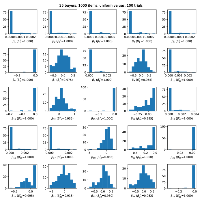
Figure 10: Distribution of $\sqrt{t}{(\beta^{\gamma}_{i}-{\beta^{*}_{i}})}$ for all $i\in[n]$. Non-normality and fast convergence for buyers with ${\beta^{*}_{i}}=1$. Uniform values.

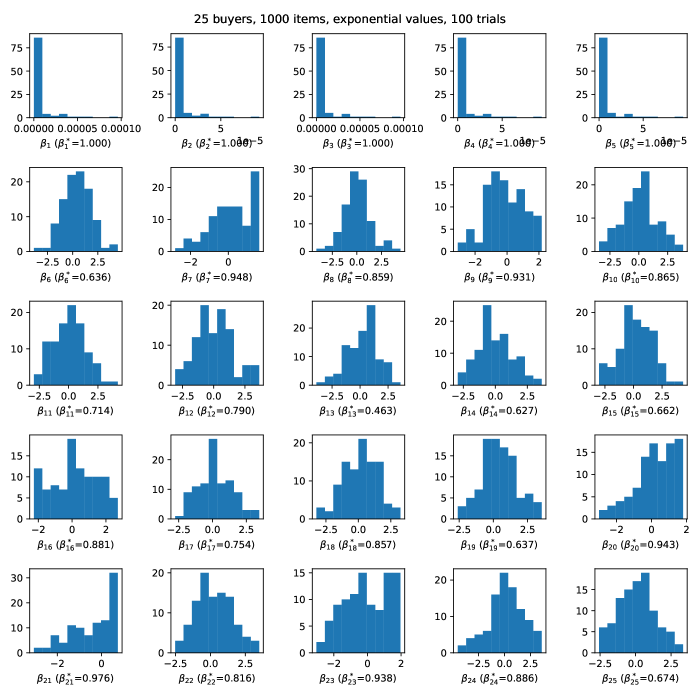
Figure 11: Distribution of $\sqrt{t}{(\beta^{\gamma}_{i}-{\beta^{*}_{i}})}$ for all $i\in[n]$. Non-normality and fast convergence for buyers with ${\beta^{*}_{i}}=1$. Exponential values.

Figure 2 shows five out of 25 distributions for pacing multipliers. Full plots for all three distributions are given in Figures 10, 11 and 12. We see that (i) if ${\beta^{*}_{i}}<1$ then the finite sample distribution is close to a normal distribution, and (ii) if ${\beta^{*}_{i}}=1$ (or very close to $1$, such as $\beta_{14,21}$ in the uniform value plots, $\beta_{20,23}$ in exponential), the finite sample distribution puts most of the probability mass at 1. For cases where ${\beta^{*}_{i}}$ is close, but not very close, to 1, we need to further increase the number of items to observe normality.

6.2 Semi-real Experiment: Nash Social Welfare Estimation in Instagram Notification System

Notifications are important in enhancing the user experience and user engagement in mobile apps. Nevertheless, an excessive barrage of notifications can be disruptive for users. Typically, a mobile application has various notification types, overseen by separate teams, each with potentially conflicting objectives. And so it is necessary to regulate notifications and send only those of most value to users. Kroer et al. (2023b) propose to use Fisher market equilibrium-based methods to efficiently send notifications, where they treat the opportunity to send a user a notification as an item, and different types of notifications as buyers. In this section, we use the inference method developed in Section 4.3 to quantify uncertainty in equilibrium-based notification allocation methods.

The data. The dataset released by Kroer et al. (2023b) contains about $400,000$ generated notifications of four types for a subset of about $60,000$ Instagram users from September 14–23, 2022. The four types of notifications (buyers) are likes, daily digest of stories, feed suite organic campaign (notification about new posts on the user’s feed), and comments subscribed. The value $v_{i}(\theta)$ of a notification type $i$ to a user $\theta$ at a specific time is predicted by the platform’s algorithm and available in the dataset as a numerical value in $[0,1]$. The budgets of notification types are also given. For a user-notification type pair, we average over the whole time window and use the average to represent $v_{i}(\theta)$, resulting in a user-notification type matrix. However, even after aggregation over time, there are lots of missing values, i.e., many users do not have every notification type generate a potential notification.

Value imputation and simulation by the Gaussian copula. We assume the values in the notification system admit the following representation. There exists unique monotone functions $f_{i}:{\mathbb{R}}\to[0,1]$, such that $(v_{1},\dots,v_{4})=(f_{1}(Z_{1}),\dots,f_{4}(Z_{4}))$, where $Z=[Z_{1},\dots,Z_{4}]$ follows a multivariate Gaussian distribution with standard normal marginals. Such an assumption is equivalent to assuming the value distribution possesses a Gaussian copula (Zhao and Udell 2020, Lemma 1 and Liu et al. 2009, Lemma 1). Given this representation, we propose a two-step simulation method. In the first step, we learn the monotone functions by matching the quantiles of values with the quantiles of a standard normal. We use isotonic regression to learn the monotone functions. Second, given the learned functions $\hat{f}_{i}$ and inverses $\hat{f}_{i}^{-1}:[0,1]\to{\mathbb{R}}$, we transform $v_{i}$ to $\hat{f}_{i}^{-1}(v_{i})$, and compute the covariance matrix of $\hat{f}_{i}^{-1}(v_{i})$, denoted $\hat{\Sigma}$. Even though some values are missing, the covariance $\Sigma$ can still be estimated by $\hat{\Sigma}$ if values are missing at random. Now to simulate a new item for buyers, we draw $Z\sim N(0,\hat{\Sigma})$, and return $[\hat{f}_{1}(Z_{1}),\dots,\hat{f}_{4}(Z_{4})]^{\top}$ as the value. There are multiple advantages to this method. First, the dependence structure of the available dataset is preserved. Second, the generated values are within the range $[0,1]$ as the original data are. Third, the marginal distribution of values are also preserved in the simulated data.

As a final step to mimic realistic data, since some users may turn off notifications of certain types, the values of those notifications will be zero. We simulate this by setting certain values to zero according to the sparsity pattern in the original dataset. See Figure 3 for a comparison between original dataset and simulated data.

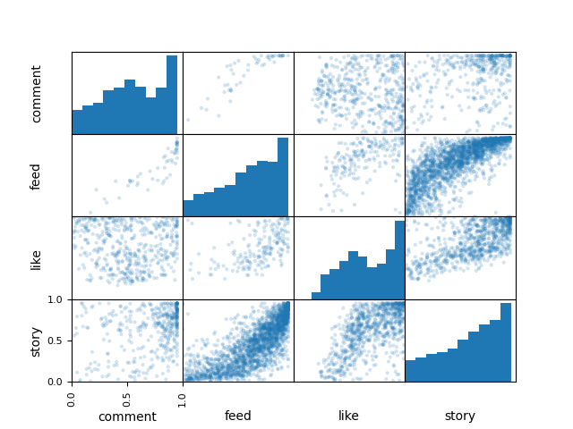
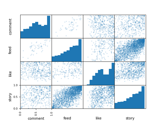
Figure 3: The fair notification allocation data. Left: original data with missing values. Right: simulated data.

Setup and results. We apply the confidence interval in Theorem 4.9 and study the coverage properties. The nominal coverage rate is set to 95%. First, we do see that even for a small sample size of 100, the nominal coverage rate is achieved. And as we increase the size of markets $t$, the coverage maintains at around 95% and the width of the CI shrinks roughly at the rate $1/\sqrt{t}$.

items	(coverage rate, width of CI)
100	(0.94, 0.88)
200	(0.95, 0.63)
400	(0.93, 0.43)
600	(0.97, 0.35)

Table 2: Coverage rate of log Nash social welfare in fair notification allocation. To help interpret the CI width, the log Nash social welfare in the limit market is around -16.

6.3 Semi-real Experiment: A/B Testing of Revenue in First-Price Auction Platforms

In this section we apply our revenue estimation method to a real-world dataset, the iPinYou dataset (Liao et al. 2014). The iPinYou dataset (Liao et al. 2014) contains raw log data of the bid, impression, click, and conversion history on the iPinYou platform in the weeks of March 11–17, June 8–15 and October 19–27. We use the impression and click data of 5 advertisers on June 8, 2013, containing a total of 1.8 million impressions and 1,200 clicks. As in the main text, let $i\in\{1,2,3,4,5\}$ index advertisers (buyers) and let $\tau$ index impressions/users (items in FPPE terminology). The five advertiser are labeled by number and their categories are given: 1459 (Chinese e-commerce), 3358 (software), 3386 (international e-commerce) and 3476 (tire). From the raw log data, the following dataset can be extracted. The response variable is a binary variable ${\small\textsc{{click}}}_{i}^{\tau}\in\{0,1\}$ that indicates whether the user clicked the ad or not. The relevant predictors include a categorical variable Adexchange of three levels that records from which ad-exchange the impression was generated, a categorical variable Region of 35 levels indicating provinces of user IPs, and finally 44 boolean variables, each a Usertag, indicating whether a user belongs to certain user groups defined based on demographic, geographic and other information. We select the top-10 most frequent user tags and denote them by ${\small\textsc{{Usertag}}}_{1},\dots,{\small\textsc{{Usertag}}}_{10}\in\{0,1\}$. Both Adexchange and Usertag are masked, and we do not know their real-world meaning.

Simulate advertisers with logistic regression. The raw data contains only five advertisers. In order to simulate new realistic advertiser, we logistic regression and then perturb the fitted coefficients to generate more advertisers. We posit the following logistic regression model for click-through rates (CTRs). For a user $\tau$ that saw the ad of advertiser $i$, the click process is governed by

$${\small\textsc{{CTR}}}_{i}^{\tau}={\mathbb{P}}({\small\textsc{{click}}}_{i}^{\tau}=1\,|\,{\theta^{\tau}})=\frac{1}{1+\exp(w_{i}^{\top}\theta^{\tau})},$$

$$\theta^{\tau}=[1,{\small\textsc{{Adexchange}}}_{2},{\small\textsc{{Adexchange}}}_{3},{\small\textsc{{Region}}}_{2},\dots,{\small\textsc{{Region}}}_{35},{\small\textsc{{Usertag}}}_{1},\dots,{\small\textsc{{Usertag}}}_{10}]\in\{1\}\times\{0,1\}^{46}$$

where the weight vectors $w_{i}\in{\mathbb{R}}^{47}$ are the coefficients to be estimated from the data. Note that ${\small\textsc{{Adexchange}}}_{1}$ and ${\small\textsc{{Region}}}_{1}$ are absorbed in the intercept. By running 5 logistic regressions, we obtain regression coefficients $w_{1},w_{2},\dots,w_{5}$. To visualize the fitted regression, in Figure 4 we show the estimated click-through rate distributions of the five advertisers. The diagonal plots are the histogram of CTRs, and the off-diagonal panels are the pair-wise scatter plots of CTRs. To generate more advertisers, we take a convex combination of the coefficients $w_{i}$’s, add uniform noise, and obtain a new parameter, say $w^{\prime}$. Given an item, the CTR of the newly generated advertisers will be $\frac{1}{1+\exp(\theta^{\top}w^{\prime})}$. The value distribution is the historical distribution of the simulated advertisers’ predicted CTRs of the 1.8 million impressions.

6.3.1 Revenue Coverage

Setup. In this section we aim to produce confidence interval of the revenue with the CI constructed from Eq. 26. Firstly, the sum equals $n$ times the average price-per-utility of advertisers, a measure of efficiency of the system. Secondly, since most quantities in FPPE, such as revenue and social welfare, are smooth functions of pacing multipliers , being able to perform inference about a linear combination of $\beta$’s indicates the ability to infer first-order estimates of those quantities.

An experiment has parameters $(t,n,d,\alpha)$. Here $t\in\{100,300,500\}$ is the number of items and $n\in\{10,20,30,50\}$ the number of advertisers. Parameter $d$ is the exponent of the finite-difference stepsize $\varepsilon_{t}$ in Eq. 22, i.e, $\varepsilon_{t}=t^{-d}$. We try $d$ over the grid $\{0.4,0.3,0.2,0.1,0.05\}$. Finally, $\alpha\in\{0.1,0.3,0.5\}$ is the proportion of advertisers that are not budget-constrained (i.e., $\beta=1$). To control $\alpha$ in the experiments, we select budgets as follows. Give infinite budgets to the first $\lfloor\alpha n\rfloor$ advertisers. Initialize the rest of the advertisers’ budgets randomly, and keep decreasing their budgets until their pacing multipliers are strictly less than 1. In the experiment $(t,n,d,\alpha)$, we first compute the pacing multiplier in the limit market using dual averaging (Xiao 2010, Gao et al. 2021, Liao et al. 2022). Then we sample one FPPE by drawing values from the synthetic value distribution obtained previously. Now given one FPPE, apply the formula in Eq. 26 to construct CI and record coverage. The reported coverage rate for an experiment with parameters $(t,n,d,\alpha)$ is averaged over 100 FPPEs.

Results. Representative results are presented in Table 3; we present the full table in Table 6. As the number of item increases, we observe the empirical coverage rate achieving the nominal 90% coverage rate, while the width of confidence interval is narrowing. We also observe that the confidence interval is robust against the Hessian estimation and the proportion of unpaced buyers; for different choices of exponent in the differencing stepsize ($\varepsilon_{t}$ in Eq. 22) and proportion of unpaced buyers ($\alpha$), the coverage performance remains similar.

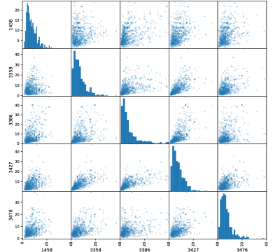
Figure 4: Click-through rate (in basis points, i.e. 0.01%) distributions from logistic regression.

Table 3: Coverage of revenue CI. $\alpha$ = proportion of $\beta_{i}=1$, $d$ is the exponent in finite difference stepsize $\epsilon_{t}=t^{-d}$.

	buyers	20				50				80
	$\alpha$	0.05	0.10	0.20	0.30	0.05	0.10	0.20	0.30	0.05	0.10	0.20	0.30
$d$	items
0.40	100	0.79 (1.72)	0.79 (1.82)	0.93 (1.87)	0.9 (1.81)	0.87 (1.84)	0.81 (1.91)	0.89 (1.82)	0.88 (2.00)	0.81 (1.89)	0.89 (1.89)	0.97 (1.97)	0.9 (1.95)
	200	0.88 (1.33)	0.88 (1.36)	0.87 (1.35)	0.9 (1.34)	0.88 (1.32)	0.93 (1.36)	0.89 (1.37)	0.94 (1.40)	0.87 (1.37)	0.93 (1.37)	0.88 (1.42)	0.86 (1.42)
	400	0.84 (0.93)	0.88 (0.99)	0.93 (0.99)	0.91 (0.98)	0.9 (0.95)	0.94 (0.98)	0.92 (0.98)	0.84 (1.00)	0.88 (0.97)	0.85 (0.98)	0.86 (1.01)	0.85 (1.01)
	600	0.89 (0.76)	0.88 (0.79)	0.9 (0.81)	0.89 (0.80)	0.8 (0.77)	0.87 (0.80)	0.81 (0.80)	0.92 (0.83)	0.86 (0.80)	0.83 (0.80)	0.97 (0.83)	0.89 (0.83)

6.3.2 Treatment Effect Coverage

Setup. In this experiment, we fix the differencing stepsize in Hessian estimation to be $\varepsilon_{t}=t^{-0.4}$ and the proportion of unpaced buyers to be 30%, which is a realistic number for real-world auction platforms.

An experiment has parameters $(t,n,\pi)$, where $t$ is the number of items, $n$ the number of users, and $\pi$ the treatment probability (see Section 5.4). To model treatment application, we use the shift of value distribution. Choose two sets of logistic regression parameters, $\{w_{i}(0)\}_{i}$ and $\{w_{i}(1)\}$. Then if a user $\theta$ is applied treatment $\omega\in\{0,1\}$, then its value to buyer $i$ will be $1/(1+\exp(w_{i}(\omega)^{\top}\theta))$, $i\in[n]$. In an experiment, the limit revenues in the two limit markets ${\textsf{{FPPE}}}(b,v(0),s,\Theta)$ and ${\textsf{{FPPE}}}(b,v(1),s,\Theta)$, and the limit treatment effect will be calculated first. Then we perform the a/b test experiments 100 times, and construct 100 CIs for the treatment effect. We report coverage rates and widths of CIs.

Results. Representative results are presented in Table 4; in Table 5 we present the full results. First, the overall coverage rates across different market setups and treatment probabilities $\pi$ are around the nominal 90%, and the width of confidence interval shrinks as sample size grows. Second, when the number of items is sufficiently large (say over 400), we observe a $U$-shape relationship between the width of CI and treatment probability $\pi$; the CI widths are wider when $\pi$ is close to the extreme points (say 0.1 and 0.9) than when $\pi$ stays away from the extreme points. This is explained by the treatment effect variance formula in Theorem 5.6. Holding the two variances fixed, the treatment effect variance tends to infinity if we send $\pi\to 0$ or $1$.

Table 4: Coverage of treatment effect. $\pi$ = treatment probability, the finite difference stepsize $\epsilon_{t}=t^{-0.4}$, proportion of unpaced buyers $\beta_{i}=1$ is 30%

	items	100	200	400	600
buyers	$\pi$
50	0.1	0.88 (8.45)	0.88 (4.75)	0.92 (1.87)	0.88 (1.54)
	0.3	0.95 (3.49)	0.96 (2.37)	0.86 (1.28)	0.93 (1.03)
	0.5	0.92 (3.76)	0.95 (5.05)	0.9 (1.26)	0.94 (0.98)
	0.7	0.85 (3.10)	0.95 (2.27)	0.98 (1.85)	0.95 (1.28)
	0.9	0.76 (3.36)	0.87 (2.87)	0.92 (2.78)	0.96 (9.33)

7 Conclusion

We introduced a theory of statistical inference for Fisher markets, resource allocation systems that deploy the CEEI mechanism, and first-price auction platforms. We showed that quantities observed in the finite market equilibrium observed from these systems are good estimators of their corresponding limit market values. We presented convergence rate results, asymptotic distribution characterizations, local minimax optimality results, and constructed confidence interval tools. Finally, we showed how to use these tools to develop a theory of statistical inference in A/B testing under competition effects.

A few open questions remain. In practice, the item arrival process exhibits nonstationarity and seasonality. A set of statistical theory for LFM and FPPE that incorporates temporal dependence is desirable. It would also be desirable to design a notion of online confidence intervals for the limit market, since, in practice, items arrive on the system sequentially. For FPPE we assumed the absence of degenerate buyers in Section 5.2. A fully general asymptotic and inferential theory for FPPE is also interesting. Finally, we restricted our attention to the first-price setting. In practice, second-price auctions are also widespread. A theory of statistical inference for second-price auctions is also desirable, though we expect it to be significantly weaker, due to computational complexity barriers, as well as non-uniqueness issues.

This research was supported by the Office of Naval Research awards N00014-22-1-2530 and N00014-23-1-2374, and the National Science Foundation awards IIS-2147361 and IIS-2238960. This work has been presented in Conference on Neural Information Processing Systems (2022), International Conference on Machine Learning (2023), Sequential Markets and Mechanism Design session in INFORMS annual meeting (2023) Stanford Rising Star Workshop (2024), Workshop on Marketplace Innovation (2024) for helpful discussion, and invited for presentation by the Ads Experimentation team at Meta. We thank attendees of these workshops and conferences for many helpful discussions.

Proofs for Analytical Properties of the Dual Objective

8 Analytical Properties of the Dual Objective

8.1 Formal Statements

We provide three sufficient conditions in Theorem 3.2. Based on the differentiability characterization, it is natural to search for a stronger form of Eq. 8 and hope that such a refinement could lead to second-order differentiability. Condition (i) gives two such refinements. Condition (ii) is motivated by the idea that expectation operator tends to produce smooth functions. The exact smoothness requirement is presented in the appendix, which we show is easy to verify for several common distributions. Finally, Condition (iii) considers the linear-valuations setting of Gao and Kroer (2022), where the authors provide tractable convex programs for computing the infinite-dimensional equilibrium. Here we give another interesting properties of this setup by showing that the dual objective is $C^{2}$. Piecewise linear value functions are discussed in the appendix.

The tied buyers for an item will be useful for later discussions. Let $I(\beta,\theta)=\argmax_{i}{\beta_{i}v_{i}(\theta)}$ be the set of maximizing indices, which could be non-unique. We say there is no tie for item $\theta$ at $\beta$ if $I(\beta,\theta)$ is single-valued, in which case we use $i(\beta,\theta)$ to denote the unique maximizing index. Moreover, by Theorem 3.50 from Beck (2017), the subgradient $\partial_{\beta}f(\theta,\beta)$ is the convex hull of the set $\{v_{i}e_{i},i\in I(\beta,\theta)\}$. When $I(\beta,\theta)$ is single-valued, the subgradient set is a singleton, and thus $f$ is differentiable.

Markets with sufficient bid gap

A natural idea is to search for a stronger form of Eq. 8 and hope that such a refinement could lead to second-order differentiability. In particular, this section is concerned with statement (i) of Theorem 3.2. First we show the condition based on the expectation.

Theorem 8.1

Suppose $H$ is differentiable in a neighborhood of $\beta^{*}$ and

$${\mathbb{E}}\bigg{[}\frac{1}{{\mathsf{{bidgap}}}(\beta^{*},\theta)}\bigg{]}=\int_{\Theta}\frac{1}{{\mathsf{{bidgap}}}(\beta^{*},\theta)}s(\theta)\mathop{}\!\mathrm{d}\theta<\infty\;,$$ (INT)

then $H$ is twice differentiable at $\beta^{*}$. Furthermore, it holds $\nabla^{2}{\bar{f}}(\beta^{*})=0$ and $\nabla^{2}H(\beta^{*})={\operatorname*{diag}}(b_{i}/({\beta^{*}_{i}})^{2})$.

Proof in Section 8.2.

We compare the integrability condition in the above theorem with Eq. 8. Both Eq. INT and Eq. 8 can be interpreted as a form of robustness of the market equilibrium. The quantity ${\mathsf{{bidgap}}}(\beta,\theta)$ measures the advantage the winner of item $\theta$ has over other losing bidders. The larger ${\mathsf{{bidgap}}}(\beta,\theta)$ is, the more slack there is in terms of perturbing the pacing multiplier before affecting the allocation at $\theta$. In contrast to Eq. 8 which only imposes an item-wise requirement on the winning margin, the above assumption requires the margin exists in a stronger sense. Concretely, such a moment condition on the margin function $\epsilon$ represents a balance between how small the margin could be and the size of item sets for which there is a small winning margin.

Second we consider the condition based on the essential supremum. For any buyer $i$ and her winning set $\Theta_{i}^{*}$, there exists a positive constant ${\epsilon}_{i}>0$ such that

$${\beta^{*}_{i}}v_{i}(\theta)\geq\max_{k\neq i}\beta^{*}_{k}v_{k}(\theta)+{\epsilon}_{i}\,,\forall\theta\in\Theta_{i}^{*}\quad\Leftrightarrow\quad\operatorname*{ess\,sup}_{\theta\in\Theta}1/{\mathsf{{bidgap}}}(\beta,\theta)<K<\infty$$ (GAP)

It requires that the buyer wins the items without tying bids uniformly over the winning item set. The existence of a constant $K<\infty$ such that $1/{\mathsf{{bidgap}}}(\beta,\theta)<K$ for almost all items makes a stronger requirement than Eq. INT. From a practical perspective, it is also evidently a very strong assumption: for example, it won’t occur with many natural continuous valuation functions. Instead, the condition requires the valuation functions to be discontinuous at the points in $\Theta$ where the allocation changes. Empirically, since $\beta^{\gamma}$ is a good approximation of $\beta^{*}$ for a market of sufficiently large size, Eq. GAP can be approximately verified by replacing $\beta^{*}$ with $\beta^{\gamma}$. As a trade-off, Eq. INT is a weaker condition than Eq. GAP but is harder to verify in practical application.

Below we present two examples where Eq. INT holds.

Example 8.2 (Discrete Values)

Suppose the values are supported on a discrete set, i.e., $[v_{1},\dots,v_{n}]\in\{V_{1},\dots,V_{K}\}\subset{\mathbb{R}^{n}}$ a.s. Suppose there is no tie for each item at $\beta^{*}$. Then Eq. GAP and thus Eq. INT hold.

Example 8.3 (Continuous Values)

Here we give a numeric example of market with two buyers where Eq. INT holds. Suppose the values are uniformly distributed over the sets $\{v\geq 0:v_{2}\leq 1,v_{2}\geq 2v_{1}\}$ and $\{v\geq 0:v_{1}\leq 1,v_{2}\leq\frac{1}{2}v_{1}\}$. See Figure 5 for an illustration. By calculus, we can show the map ${\bar{f}}(\beta)={\mathbb{E}}[\max\{v_{1}\beta_{1},v_{2}\beta_{2}\}]$ is

$${\bar{f}}(\beta)=\begin{cases}\big{(}\frac{5}{12}-\frac{1}{3}\frac{\beta_{1}}{\beta_{2}}\big{)}\beta_{1}+\frac{2\beta_{2}}{3\beta_{1}}\beta_{2}&\text{if $\beta_{2}\geq 2\beta_{1}$}\\ \frac{1}{3}(\beta_{1}+\beta_{2})&\text{if $\tfrac{1}{2}\beta_{1}<\beta_{2}<2\beta_{1}$}\\ \big{(}\frac{5}{12}-\frac{1}{3}\frac{\beta_{2}}{\beta_{1}}\big{)}\beta_{2}+\frac{2\beta_{1}}{3\beta_{2}}\beta_{1}&\text{if $\beta_{2}\leq\frac{1}{2}\beta_{1}$}\end{cases}\;.$$

Next, we derive the Hessian of ${\bar{f}}$. On $\{\tfrac{1}{2}\beta_{1}<\beta_{2}<2\beta_{1}\}$ we have $\nabla^{2}{\bar{f}}=0$. In the region $\{\beta_{2}>2\beta_{1}\}$, the Hessian is

$$\nabla^{2}{\bar{f}}(\beta)=\begin{bmatrix}\frac{2\,{\beta_{2}}^{2}}{3\,{\beta_{1}}^{3}}&-\frac{2\,\beta_{2}}{3\,{\beta_{1}}^{2}}\\ -\frac{2\,\beta_{2}}{3\,{\beta_{1}}^{2}}&\frac{2}{3\,\beta_{1}}\end{bmatrix}\;.$$

The Hessian on the region $\{\beta_{2}<\frac{1}{2}\beta_{1}\}$ has a completely symmetric expression by switching $\beta_{1}$ and $\beta_{2}$. The Hessian can also be derived using formulas in Section 8.3. From here we can see the function ${\bar{f}}$ is $C^{2}$ except on the lines $\beta_{2}=2\beta_{1}$ and $\beta_{2}=\beta_{1}/2$.

Consider $\beta$ on $B=\{\beta>0:\frac{1}{2}\beta_{1}<\beta_{2}<2\beta_{1}\}$. Eq. INT holds. And that $\nabla^{2}{\bar{f}}(\beta)=0$ on $B$, which agrees with Theorem 8.1.

Consider $\beta$ in the interior of region $\{\beta>0:\beta_{2}>2\beta_{1}\}$. The function ${\bar{f}}$ is twice continuously differentiable but Eq. INT does not hold.

Consider $\beta$ on the ray $\{\beta>0:\beta_{2}=2\beta_{1}\}$. For these $\beta$’s the set $\{\theta:{\mathsf{{bidgap}}}(\beta,\theta)=0\}$ is measure zero and yet $\nabla^{2}{\bar{f}}(\beta)$ is not twice differentiable at these $\beta$’s. This implies Eq. 8 does not necessarily imply twice differentiability.

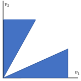
Figure 5: Value distribution in Example 8.3

Markets with linear values

Now we consider the condition (iii) of Theorem 3.2: linear valuations. We adopt the setup in Section 4 from Gao and Kroer (2022) where we impose an extra normalization on the values; the reasoning extends to the cases where at any point there are at most two lines intersecting at that point. Suppose the item space is $\Theta=[0,1]$ with supply $s(\theta)=1$. The valuation of each buyer $i$ is linear and nonnegative: $v_{i}(\theta)=c_{i}\theta+d_{i}\geq 0$. Moreover, assume the valuations are normalized so that $\int_{[0,1]}v_{i}\mathop{}\!\mathrm{d}\theta=1\Leftrightarrow c_{i}/2+d_{i}=1$. Assume the intercepts of $v_{i}$ are ordered such that $2\geq d_{1}>\cdots>d_{n}\geq 0$.

We briefly review the structure of equilibrium allocation in this setting. By Lemma 5 from Gao and Kroer (2022), there is a unique partition $0=a^{*}_{0}<a_{1}^{*}<\cdots<a_{n}^{*}=1$ such that buyer $i$ receives $\Theta_{i}=\left[a_{i-1}^{*},a_{i}^{*}\right]$. In words, the item set $[0,1]$ will be partitioned into $n$ segments and assigned to buyers $1$ to $n$ one by one starting from the leftmost segments. Intuitively, buyer 1 values items on the left of the interval more than those on the right, which explains the allocation structure. Moreover, the equilibrium prices $p^{*}(\cdot)$ are convex piecewise linear with exactly $n$ linear pieces, corresponding to intervals that are the pure equilibrium allocations to the buyers.

Theorem 8.4

In the market set up as above, the dual objective $H$ is $C^{2}$ at $\beta^{*}$.

Proof in Section 8.2.

The above result also extends to most cases of piecewise linear (PWL) valuations discussed in Section 4.3 of Gao and Kroer (2022)). In the PWL setup there is a partition of $[0,1]$, $A_{0}=0\leq A_{1}\leq\cdots\leq A_{K-1}\leq A_{K}=1$, such that all $v_{i}(\theta)$’s are linear on $[A_{k-1},A_{k}]$. At the equilibrium of a market with PWL valuations, we call an item $\theta$ an allocation breakpoint if there is a tie, i.e., $I(\beta^{*},\theta)=\argmax_{i}\beta_{i}{v_{i}(\theta)}$ is multivalued. Now suppose the following two conditions hold: (i) none of the allocation breakpoints coincide with any of the valuation breakpoints $\{A_{k}\}$, and (ii) at any allocation breakpoint there are exactly two buyers in a tie. Under these two conditions, one can show that in a small enough neighborhood of the optimal pacing multiplier $\beta^{*}$, the allocation breakpoints are differentiable functions of the pacing multiplier. This in turn implies twice differentiability of the dual objective by repeating the argument in the proof of Theorem 8.4. However, if either condition (i) or (ii) mentioned above breaks, the dual objective is not twice differentiable.

Markets with angularly smooth values

We first use a change of variable, and let $z=v/\|v\|_{2}$ be the projection of $v$ onto the unit sphere. It represents the angular component of the vector $v$. Let $f(v,\beta)=\max_{i}\beta_{i}{v_{i}(\theta)}$. Using a change of variable $z=v/\|v\|_{2}$ and $r=\|v\|_{2}$ and homogeneity of $f$, the integral $\int f(v,\beta)f_{v}\mathop{}\!\mathrm{d}v$ can be written as

$$\int_{S_{n}}\int_{0}^{\infty}f(rz,\beta)r^{n-1}f_{v}(rz)\mathop{}\!\mathrm{d}r\mathop{}\!\mathrm{d}z=\int_{S_{n}}f(z,\beta)\bigg{(}\int_{0}^{\infty}r^{n}f_{v}(rz)\mathop{}\!\mathrm{d}r\bigg{)}\mathop{}\!\mathrm{d}z$$ (28)

where $\mathop{}\!\mathrm{d}z$ is the surface measure on the unit ball $S_{n}$ in ${\mathbb{R}^{n}}$. From this representation, it is not unreasonable to say that if $\int_{0}^{\infty}r^{n}f_{v}(rz)\mathop{}\!\mathrm{d}r$ is a smooth function of the angular component $z$, then ${\bar{f}}(\beta)$ will also be a smooth function of $\beta$. Taking $v_{i}=rz_{i}$, $v_{k}=z_{k}/z_{i}$, and so $\int_{0}^{\infty}r^{n}f_{v}(rz)\mathop{}\!\mathrm{d}r=\int_{0}^{\infty}v_{i}^{n}f_{v}(v_{i}v_{1},v_{i}v_{2},\dots,v_{i},\dots,v_{i}v_{n})\mathop{}\!\mathrm{d}v_{i}/(z_{i})^{n}$. So equivalently we require smoothness of $v_{-i}\mapsto\int_{0}^{\infty}v_{i}^{n}f_{v}(v_{i}v_{1},v_{i}v_{2},\dots,v_{i},\dots,v_{i}v_{n})\mathop{}\!\mathrm{d}v_{i}$.

Now we make this precise. First we introduce some extra notations. For each $i\in[n]$, define the map $\sigma_{i}:{\mathbb{R}^{n}_{+}}\to{\mathbb{R}^{n}_{+}}$,

$$\sigma_{i}(v)=[v_{1}v_{i},\,\dots,\,v_{i-1}v_{i},\,v_{i},\,v_{i+1}v_{i},\,\dots,\,v_{n}v_{i}]^{\top}$$

for $i\in[n]$, which multiplies all except the $i$-th entry of $v$ by $v_{i}$.

Definition 8.5 (Angular regularity)

Let $f:{\mathbb{R}^{n}_{+}}\to{\mathbb{R}_{+}}$ be the probability density function (w.r.t. the Lebesgue measure) of a positive-valued random vector with finite first moment. We say the density $f$ is angularly regular if for all $h_{i}(v_{-i})=\int_{0}^{\infty}f\big{(}\sigma_{i}(v)\big{)}v_{i}^{n}\mathop{}\!\mathrm{d}v_{i}\,$, $i\in[n]$, it holds (i) $h_{i}$ is continuous on ${\mathbb{R}}^{n-1}_{++}$, and (ii) all lower dimensional density functions of $h_{i}$ are continuous (treating $h_{i}$ as a scaled probability density function).

Theorem 8.6

Assume the random vector $[v_{1},\dots,v_{n}]:\Theta\to{\mathbb{R}^{n}_{+}}$ has a distribution absolutely continuous w.r.t. the Lebesgue measure on ${\mathbb{R}^{n}}$ with density function $f_{v}$. If $f_{v}$ is angularly regular, then $H$ is twice continuously differentiable on ${\mathbb{R}^{n}_{++}}$.

Proof in Section 8.2.

The above regularity conditions are easy to verify when the values are i.i.d. draws from a distribution. In that case, many smooth distributions supported on the positive reals fall under the umbrella of the described regularity. Below we examine three cases: the truncated Gaussian distribution, the exponential distribution and the uniform distribution.

When values are i.i.d. truncated standard Gaussians, the joint density $f(v)=c_{1}\prod_{i=1}^{n}\exp(-v_{i}^{2}/2)$ and $h_{i}(v_{-i})=c_{1}\int_{\mathbb{R}_{+}}v_{i}^{n}\exp({-\frac{1}{2}v_{i}^{2}(1+\sum_{k\neq i}v_{k}^{2})})\mathop{}\!\mathrm{d}v_{i}=c_{2}(\sum_{k\neq i}v_{k}^{2})^{-n/2},$ which are regular. Here $c_{i}$, $i=1,2$, are appropriate constants. Similarly, for the i.i.d. exponential case with the rate parameter equal to one, the density $f(v)=\prod_{i=1}^{n}\exp(-v_{i})$ and $h_{i}(v_{-i})=(\sum_{k\neq i}v_{k})^{-n}$ satisfy the required continuity conditions. Finally, suppose the values are i.i.d. uniforms on $[0,1]$. The joint density is $f(v)=\prod_{i=1}^{n}{\mathds{1}}\{0<v_{i}<1\}$ and for example, if $i=1$, $h_{1}(v_{-1})=(\min\{1,v_{2}^{-1},\dots,v_{n}^{-1}\})^{n+1}/(n+1)$, which also satisfies the required continuity conditions.

8.2 Proofs

Proof 8.7 (Proof of Theorem 3.1)

Recall $f(\theta,\beta)=\max_{i}\beta_{i}{v_{i}(\theta)}$. Note $f$ is differentiable at $\beta$ if and only if ${\mathsf{{bidgap}}}(\beta,\theta)>0$. Let $\Theta_{\mathrm{diff}}(\beta)=\{\theta:f(\theta,\beta)\text{ is continuously differentiable at $\beta$}\}$. Then

$$\Theta_{\mathrm{diff}}(\beta)=\bigg{\{}\theta:\frac{1}{{\mathsf{{bidgap}}}(\beta,\theta)}<\infty\bigg{\}}=\{\theta:I(\beta,\theta)\text{ is single-valued}\}\;.$$

By Proposition 2.3 from Bertsekas (1973) we know ${\bar{f}}(\beta)={\mathbb{E}}[f(\theta,\beta)]=\int_{\Theta}f(\theta,\beta)s(\theta)\mathop{}\!\mathrm{d}\theta$ is differentiable at $\beta$ if and only if $\int{\mathds{1}}(\Theta_{\mathrm{diff}}(\beta))s(\theta){\mathop{}\!\mathrm{d}\theta}=1$. From here we obtain Theorem 3.1.

Remark 8.8

Suppose Eq. 8 holds in a neighborhood $N$ of $\beta^{*}$, i.e., $\frac{1}{{\mathsf{{bidgap}}}(\beta,\theta)}$ is finite a.s. for each $\beta\in N$, then by Theorem 3.1 we know $H$ is differentiable on $N$. In fact, a stronger statement holds: $H$ is continuously differentiable on $N$. See Proposition 2.1 from Shapiro (1989).

Remark 8.9 (Comment on Theorem 3.1)

We briefly discuss why differentiability is related to the gap in buyers’ bids. Recall ${\bar{f}}(\beta)={\mathbb{E}}[\max_{i}\beta_{i}v_{i}(\theta)]$. Let $\delta\in{\mathbb{R}^{n}_{+}}$ be a direction with positive entries, and let $I(\beta,\theta)=\argmax_{i}{\beta_{i}v_{i}(\theta)}$ be the set of winners of item $\theta$ which could be multivalued. Consider the directional derivative of ${\bar{f}}$ at $\beta$ along the direction $\delta$:

$$\lim_{t\downarrow 0}{\mathbb{E}}\bigg{[}\frac{\max_{i}(\beta_{i}+t\delta_{i})v_{i}(\theta)-\max_{i}\beta_{i}v_{i}(\theta)}{t}\bigg{]}$$

$$={\mathbb{E}}\bigg{[}\lim_{t\downarrow 0}\frac{\max_{i}(\beta_{i}+t\delta_{i})v_{i}(\theta)-\max_{i}\beta_{i}v_{i}(\theta)}{t}\bigg{]}$$

$$={\mathbb{E}}\Big{[}\max_{i\in I(\beta,\theta)}v_{i}(\theta)\delta_{i}\Big{]}\;,$$

where the exchange of limit and expectation is justified by the dominated convergence theorem. Similarly, the left limit is

$$\lim_{t\uparrow 0}{\mathbb{E}}\bigg{[}\frac{\max_{i}(\beta_{i}+t\delta_{i})v_{i}(\theta)-\max_{i}\beta_{i}v_{i}(\theta)}{t}\bigg{]}={\mathbb{E}}\Big{[}\min_{i\in I(\beta,\theta)}v_{i}(\theta)\delta_{i}\Big{]}\;.$$

If there is a tie at $\beta$ with positive probability, i.e., the set $I(\beta,\theta)$ is multivalued for a non-zero measure set of items, then the left and right directional derivatives along the direction $\delta$ do not agree. Since differentiability at a point $\beta$ implies existence of directional derivatives, we conclude differentiability implies Eq. 8.

Proof 8.10 (Proof of Theorem 8.1)

By assumption, there is a neighborhood of $\beta^{*}$, say $N$, on which $H$ is differentiable. By Theorem 3.1, for $\beta\in N$, $f$ is differentiable at $\beta$ almost surely. Define $G:N\times\Theta\to{\mathbb{R}^{n}_{+}}$, $G(\beta,\theta)=\nabla f(\theta,\beta)$. To compute the Hessian w.r.t. the first term ${\bar{f}}$, we look at the limit

$$\lim_{h\to 0}{\mathbb{E}}\bigg{[}\frac{G(\beta^{*}+h,\theta)-G(\beta^{*},\theta)}{\|h\|}\bigg{]}\;.$$ (29)

Suppose we could exchange expectation and limit in Eq. 29, then the above expression would become zero: for a fixed $\theta$, since Eq. 8 holds at $\beta^{*}$, i.e, ${\mathsf{{bidgap}}}(\beta^{*},\theta)>0$, we apply Lemma 8.11 and obtain $\lim_{h\to 0}{(G(\beta^{*}+h,\theta)-G(\beta^{*},\theta))}/{\|h\|}=0.$ This implies that $H$ is twice differentiable at $\beta^{*}$ with Hessian $\nabla^{2}H(\beta^{*})=\nabla^{2}\Psi(\beta^{*})$. It is then natural to ask for sufficient conditions for exchanging limit and expectation.

Lemma 8.11 (${\mathsf{{bidgap}}}(\beta,\theta)$ as Lipschitz parameter of $G$)

Let $\beta,\beta^{\prime}\in N$.

• If $\|\beta-\beta^{\prime}\|_{\infty}\leq{\mathsf{{bidgap}}}(\beta,\theta)/{\bar{v}}$ then $G(\beta^{\prime},\theta)=G(\beta,\theta)$.

• It holds ${\|G(\beta^{\prime},\theta)-G(\beta,\theta)\|_{2}}{}\leq 6{\bar{v}}^{2}\cdot\frac{1}{{\mathsf{{bidgap}}}(\beta,\theta)}\|\beta^{\prime}-\beta\|_{2}$.

By Lemma 8.11, we know the ratio ${(G(\beta^{*}+h,\theta)-G(\beta^{*},\theta))}/{\|h\|}$ is dominated by $6{\bar{v}}{\mathsf{{bidgap}}}(\beta^{*},\theta)^{-1}$, which by Eq. INT is integrable. By dominated convergence theorem, we can exchange limit and expectation, and the claim follows.

Proof 8.12 (Proof of Lemma 8.11)

Note that for any $\beta$ and $\theta$ with ${\mathsf{{bidgap}}}(\beta,\theta)>0$, and any $\beta^{\prime}=\beta+h$,

$$\frac{\|G(\beta+h,\theta)-G(\beta,\theta)\|_{2}}{\|h\|_{2}}\leq 6{\bar{v}}^{2}\cdot\frac{1}{{\mathsf{{bidgap}}}(\beta,\theta)}\;.$$ (30)

To see this, we notice that on one hand, if $\|h\|_{\infty}\leq\epsilon/(3{\bar{v}})$ where $\epsilon={\mathsf{{bidgap}}}(\beta,\theta)$, then for $i=i(\beta,\theta)$ and all $\theta\in\Theta_{i}(\beta)$,

$$\beta^{\prime}_{i}v_{i}(\theta) =(\beta_{i}+h_{i})v_{i}(\theta)$$

$$\geq\beta_{i}v_{i}(\theta)-\epsilon/3$$ (A)

$$\geq\beta_{k}v_{k}(\theta)+\epsilon-\epsilon/3$$ (B)

$$\geq\beta^{\prime}_{k}v_{k}(\theta)-\epsilon/3+\epsilon-\epsilon/3\;,$$ (C)

where $(A)$ and $(C)$ use the fact $\|h\|_{\infty}\leq\epsilon/(3{\bar{v}})$, and (B) uses the definition of $\epsilon$. This implies $\argmax_{i}\beta^{\prime}_{i}{v_{i}(\theta)}=\argmax_{i}\beta_{i}{v_{i}(\theta)}$ and thus $G(\beta+h,\theta)-G(\beta,\theta)=0$. On the other hand, if $\|h\|_{\infty}>\epsilon/(3{\bar{v}})$, then $\|h\|_{2}\geq\|h\|_{\infty}>\epsilon/(3{\bar{v}})$. Using the bound $\|G\|_{2}\leq{\bar{v}}$, we obtain Eq. 30. This completes proof of Lemma 8.11.

Proof 8.13 (Proof of Theorem 8.4)

Recall the normalization on values $c_{i}/2+d_{i}=1$. By Lemma 5 from Gao and Kroer (2022), we know that at the LFM equilibrium the there exists unique breakpoints $0=a_{0}^{*}<a_{1}^{*}<\cdots<a_{n}^{*}=1$, $a^{*}_{i}=(-{\beta^{*}_{i}}d_{i}+\beta^{*}_{i+1}d_{i+1})/({\beta^{*}_{i}}c_{i}-\beta^{*}_{i+1}c_{i+1})$, such that buyer $i$ receives the item set $[a_{i-1}^{*},a_{i}^{*}]\subset\Theta=[0,1]$. Moreover, it holds

$$\beta^{*}_{1}d_{1}>\beta^{*}_{2}d_{2}>\dots>\beta^{*}_{n}d_{n}\;,$$

$$\beta^{*}_{1}c_{1}<\beta^{*}_{2}c_{2}<\dots<\beta^{*}_{n}c_{n}\;.$$

Now we consider a small enough neighborhood $N$ of $\beta^{*}$. For each $\beta\in N$, we define the breakpoint $a_{i}^{*}(\beta)=(-\beta_{i}d_{i}+\beta_{i+1}d_{i+1})/(\beta_{i}c_{i}-\beta_{i+1}c_{i+1})$ by solving for $\theta$ through $\beta_{i}(c_{i}\theta+d_{i})=\beta_{i+1}(c_{i+1}\theta+d_{i+1})$ for $i\in[n-1]$, $a_{0}^{*}(\beta)=0$, and $a_{n}^{*}(\beta)=1$. Let $\Theta_{i}(\beta)=\{\theta\in\Theta:v_{i}(\theta)\beta_{i}\geq v_{k}(\theta)\beta_{k},\forall k\neq i\}$.

Lemma 8.14

There is a neighborhood $N$ of $\beta^{*}$, so that $\Theta_{i}(\beta)=[a_{i-1}^{*}(\beta),a_{i}^{*}(\beta)]$ for $\beta\in N$.

When exists, the gradient is always $\nabla{\bar{f}}(\beta)={\sum_{i=1}^{n}}e_{i}\int{\mathds{1}}(\Theta_{i}(\beta))v_{i}(\theta)s(\theta){\mathop{}\!\mathrm{d}\theta}$. For $\beta\in N$, it further simplifies to

$$\nabla{\bar{f}}(\beta) ={\sum_{i=1}^{n}}e_{i}\int{\mathds{1}}([a_{i-1}^{*}(\beta),a_{i}^{*}(\beta)])(c_{i}\theta+d_{i})\mathop{}\!\mathrm{d}\theta$$

$$={\sum_{i=1}^{n}}e_{i}\bigg{(}\frac{c_{i}}{2}\big{(}[a_{i}^{*}(\beta)]^{2}-[a_{i-1}^{*}(\beta)]^{2}\big{)}+d_{i}\big{(}a_{i}^{*}(\beta)-a_{i-1}^{*}(\beta)\big{)}\bigg{)}\;.$$

From this we see that continuous differentiability of the breakpoints $a^{*}_{i}(\beta)$ implies continuous differentiability of $\nabla^{2}{\bar{f}}$. This finishes the proof of Theorem 8.4.

Proof 8.15 (Proof of Lemma 8.14)

We construct such a neighborhood $N$. Define

$$\delta=\min\bigg{\{}\frac{1}{2}\underaccent{\bar}{\Delta}_{\beta d}/\bar{\Delta}_{d},\frac{1}{2}\underaccent{\bar}{\Delta}_{\beta c}/\bar{\Delta}_{c},\frac{1}{4}\underaccent{\bar}{\Delta}_{a}\underaccent{\bar}{\Delta}_{\beta c}/{\bar{v}}\bigg{\}}\;,$$

where $\underaccent{\bar}{\Delta}_{a}=\min|a_{i}-a_{i-1}|$, $\underaccent{\bar}{\Delta}_{\beta c}=\min\{\beta^{*}_{i-1}c_{i-1}-\beta^{*}_{i}c_{i}\}>0$, $\bar{\Delta}_{c}=\max_{i}\{c_{i-1}-c_{i}\}>0$, and $\underaccent{\bar}{\Delta}_{\beta d}>0$ and $\bar{\Delta}_{d}>0$ are similarly defined. Let $N=\{\beta:\|\beta-\beta^{*}\|_{\infty}<\delta\}$. The neighborhood $N$ is constructed so that on $N$ it holds

$$\beta_{1}d_{1}>\beta_{2}d_{2}>\dots>\beta_{n}d_{n}\;,$$

$$\beta_{1}c_{1}<\beta_{2}c_{2}<\dots<\beta_{n}c_{n}\;,$$

$$0=a_{0}^{*}(\beta)<a_{1}^{*}(\beta)<\cdots<a_{n}^{*}(\beta)=1\;,$$

where the first inequality follows from $\delta\leq\frac{1}{2}\underaccent{\bar}{\Delta}_{\beta d}/\bar{\Delta}_{d}$, the second inequality from $\delta\leq\frac{1}{2}\underaccent{\bar}{\Delta}_{\beta c}/\bar{\Delta}_{c}$, and the third inequality follows from $\delta\leq\underaccent{\bar}{\Delta}_{a}\underaccent{\bar}{\Delta}_{\beta c}/(4{\bar{v}})$, where ${\bar{v}}=\max_{i}\sup_{\theta\in[0,1]}c_{i}\theta+d_{i}$. For $\theta\in[0,a_{1}^{*}(\beta)]$, $\max_{i}\beta_{i}(c_{i}\theta+d_{i})$ is achieved by $i=1$. Similarly for $i=2,\dots,n$. So we have shown $\Theta_{i}(\beta)=[a_{i-1}^{*}(\beta),a_{i}^{*}(\beta)]$ for $\beta\in N$.

Proof 8.16 (Proof of Theorem 8.6)

We need the following technical lemma on the continuous differentiability of integral functions.

Lemma 8.17 (Adapted from Lemma 2.5 from Wang (1985))

Let $u=[u_{1},\dots,u_{n}]\in{\mathbb{R}^{n}_{++}}$, and

$$I(u)=\int_{0}^{u_{1}}\mathop{}\!\mathrm{d}t_{1}\dots\int_{0}^{u_{n}}h(t_{1},t_{2},\dots,t_{n})\mathop{}\!\mathrm{d}t_{n}\;,$$

where $h$ is a continuous density function of a probabilistic distribution function on ${\mathbb{R}^{n}_{+}}$ and such that all lower dimensional density functions are also continuous. Then the integral $I(u)$ is continuously differentiable.

Remark 8.18

The difference between the above lemma and the original statement is that the original theorem works with density $h$ and integral function $I(u)$ both defined on ${\mathbb{R}^{n}}$, while the adapted version works with density $h$ and integral $I(u)$ defined only on ${\mathbb{R}^{n}_{++}}$.

The gradient expression is

$$\nabla{\bar{f}}(\beta)={\sum_{i=1}^{n}}e_{i}\int v_{i}{\mathds{1}}(V_{i}(\beta))f_{v}(v)\mathop{}\!\mathrm{d}v\;,$$

where the set $V_{i}(\beta)=\{v\in{\mathbb{R}^{n}_{+}}:v_{i}\beta_{i}\geq v_{k}\beta_{k},k\neq i\},i\in[n]$, is the values for which buyer $i$ wins. For now, we focus on the first entry of the gradient, i.e., $\int v_{1}{\mathds{1}}(V_{1}(\beta))f_{v}(v)\mathop{}\!\mathrm{d}v$. We write the integral more explicitly as follows. By Fubini’s theorem,

$$\int v_{1}{\mathds{1}}(V_{1}(\beta))f_{v}(v)\mathop{}\!\mathrm{d}v$$ (31)

$$=\int_{0}^{\infty}\mathop{}\!\mathrm{d}v_{1}\int_{0}^{\frac{\beta_{1}v_{1}}{\beta_{2}}}\mathop{}\!\mathrm{d}v_{2}\int_{0}^{\frac{\beta_{1}v_{1}}{\beta_{3}}}\mathop{}\!\mathrm{d}v_{3}\dots\int_{0}^{\frac{\beta_{1}v_{1}}{\beta_{n}}}\underbrace{(v_{1}f_{v}(v_{1},\dots,v_{n}))}_{=:A_{1}(v)}\mathop{}\!\mathrm{d}v_{n}\;.$$ (32)

To apply the lemma we use a change of variable. Let $t=T(v)=[v_{1},\frac{v_{2}}{v_{1}},\dots,\frac{v_{n}}{v_{1}}]$ and $v=T^{-1}(t)=[t_{1},t_{2}t_{1},\dots,t_{n}t_{1}]$. Then Eq. 32 is equal to

$$\int_{0}^{\infty}\mathop{}\!\mathrm{d}t_{1}\int_{0}^{\frac{\beta_{1}}{\beta_{2}}}\mathop{}\!\mathrm{d}t_{2}\int_{0}^{\frac{\beta_{1}}{\beta_{3}}}\mathop{}\!\mathrm{d}t_{3}\dots\int_{0}^{\frac{\beta_{1}}{\beta_{n}}}\underbrace{\big{(}t_{1}^{n}f_{v}(t_{1},t_{2}t_{1},\dots,t_{n}t_{1})\big{)}}_{=:A_{2}(t)}\mathop{}\!\mathrm{d}t_{n}\;.$$ (33)

Note ${\mathbb{E}}[v_{1}(\theta)]=\int_{\mathbb{R}^{n}_{++}}A_{1}(v)\mathop{}\!\mathrm{d}v=\int_{\mathbb{R}^{n}_{++}}A_{2}(t)\mathop{}\!\mathrm{d}t=1$. We use Fubini’s theorem and obtain

$$\lx@cref{creftype~refnum}{eq:after_change_of_var}=\int_{0}^{\frac{\beta_{1}}{\beta_{2}}}\mathop{}\!\mathrm{d}t_{2}\int_{0}^{\frac{\beta_{1}}{\beta_{3}}}\mathop{}\!\mathrm{d}t_{3}\dots\int_{0}^{\frac{\beta_{1}}{\beta_{n}}}h(t_{-1})\mathop{}\!\mathrm{d}t_{n}\;,$$

where we have defined $h(t_{-1})=\int_{\mathbb{R}_{+}}t_{1}^{n}f_{v}(t_{1},t_{2}t_{1},\dots,t_{n}t_{1})\mathop{}\!\mathrm{d}t_{1}$. By the smoothness assumption on $h$ and Lemma 8.17, we know that the map $u_{-1}\mapsto\int_{0}^{u_{2}}\mathop{}\!\mathrm{d}t_{2}\dots\int_{0}^{u_{n}}h(t_{-1})\mathop{}\!\mathrm{d}t_{n}$ is $C^{1}$ for all $u_{-1}\in{\mathbb{R}^{n-1}_{++}}$. Moreover, the map $\beta\mapsto[\frac{\beta_{1}}{\beta_{2}},\dots,\frac{\beta_{1}}{\beta_{n}}]$ is $C^{1}$. We conclude the first entry of $\nabla{\bar{f}}(\beta)$ is $C^{1}$ in the parameter $\beta$. A similar argument applies to other entries of the gradient. We complete the proof of Theorem 8.6.

8.3 Closed-form Expression for Hessian

In this section we derive closed form expression for $\nabla^{2}{\bar{f}}(\beta)$ for some $\beta\in{\mathbb{R}^{n}_{+}}$ using tools from differential geometry. Let $f_{v}(v)$ be the density of values w.r.t. the Lebesgue measure on ${\mathbb{R}^{n}}$. Let ${\mathcal{K}}=\nabla^{2}{\bar{f}}(\beta)$. Then $\nabla^{2}H(\beta)={\mathcal{K}}+{\operatorname*{diag}}(b_{i}/(\beta_{i})^{2})$. Fix a buyer $k$. Now we derive ${\mathcal{K}}_{k,h}$ for $h\in[n]$. We need to introduce a few sets. Let

$$V=\{v\in{\mathbb{R}^{n}_{+}}:\beta_{i}v_{i}\leq\beta_{k}v_{k},i\in[n]\}\;,$$

$$S_{h}=\{v\in{\mathbb{R}^{n}_{+}}:\beta_{k}v_{k}=\beta_{h}v_{h},\beta_{i}v_{i}\leq\beta_{k}v_{k},i\neq k,h\}=V\cap\{v:\beta_{k}v_{k}=\beta_{h}v_{h}\}\;,$$

$$\Pi_{h}=\{v_{-k}\in{\mathbb{R}}^{n-1}_{+}:\beta_{i}v_{i}\leq\beta_{h}v_{h},i\neq k,h\}\;.$$

Figure 6: Illustration of $V$, $S_{h}$ and $\Pi_{h}$.

The cone $V$, which we call the winning cone of buyer $k$, is the set of valuation vectors such that buyer $k$ wins under the pacing profile $\beta$. The set $S_{h}$ is a face of $V$, which represents the values for which there is a tie between buyers $k$ and $h$. It is clear $\Pi_{h}$ is the projection of $S_{h}$ onto $\{v\in{\mathbb{R}^{n}}:v_{k}=0\}$. In Figure 6 we present an illustration of these sets.

We will show that the Hessian $\mathcal{K}$ can be characterized as

$${\mathcal{K}}_{k,h}=-\frac{\beta_{h}}{\beta_{k}^{2}}\int_{\Pi_{h}}v_{h}^{2}f_{v}(v_{1},\dots,v_{k-1},\frac{\beta_{h}v_{h}}{\beta_{k}},v_{k+1},\dots,v_{n})\mathop{}\!\mathrm{d}v_{-k}\quad\text{ for }h\neq k\;,$$ (34)

$${\mathcal{K}}_{k,k}=\sum_{h\neq k}\frac{\beta_{h}^{2}}{\beta_{k}^{3}}\int_{\Pi_{h}}v_{h}^{2}f_{v}(v_{1},\dots,v_{k-1},\frac{\beta_{h}v_{h}}{\beta_{k}},v_{k+1},\dots,v_{n})\mathop{}\!\mathrm{d}v_{-k}\;.$$ (35)

The formulae indicate that only the value of $f_{v}$ on the faces $S_{h}$, $h\neq k$ matters for the Hessian.

Let $\Delta=\beta_{k}e_{k}-\beta_{h}e_{h}$ and $\Delta_{u}=\beta_{k}e_{k}-ue_{h}$ for a scalar $u$. The $k$-th entry of $\nabla{\bar{f}}(\beta)$ is $\int{\mathds{1}}(V(\beta))v_{k}f_{v}\mathop{}\!\mathrm{d}v$ and so the second-order derivative of ${\bar{f}}$ can be written as

$${\mathcal{K}}_{k,h}=\frac{\partial}{\partial\beta_{h}}\int{\mathds{1}}(V(\beta))v_{k}f_{v}\mathop{}\!\mathrm{d}v\;.$$

Define the rotation matrix

$$T_{u}=\bigg{(}I_{n}-\frac{\Delta_{u}\Delta_{u}^{\top}}{\|\Delta_{u}\|_{2}^{2}}\bigg{)}\bigg{(}I_{n}-\frac{\Delta\Delta^{\top}}{\|\Delta\|_{2}^{2}}\bigg{)}+\frac{1}{\|\Delta\|_{2}\|\Delta_{u}\|_{2}}\Delta_{u}\Delta^{\top}\;.$$

The map $T_{u}$ is a diffeomorphism that maps $\{v:\Delta^{\top}v\geq 0\}$ to the region $\{v:\Delta_{u}^{\top}v\geq 0\}$. It can be seen that $T_{u}(\Delta/\|\Delta\|_{2})=\Delta_{u}/\|\Delta_{u}\|_{2}$ and $T_{\beta_{h}}=I_{n}$. Notice that if we increase $\beta_{h}$, $h\neq k$, the face $S_{h}$ rotates inward in $V$, pivoting at the origin. By a result from Section 5 in Kim and Pollard (1990), the derivative of the volume of a parametrized region can be written as a surface integral on the boundary of the region. Concretely, in our case, we have that

$$\frac{\partial}{\partial\beta_{h}}\int{\mathds{1}}(V(\beta))v_{k}f_{v}\mathop{}\!\mathrm{d}v=\int{\mathds{1}}(S_{h})v_{k}f_{v}n(v)^{\top}\Big{(}\frac{\partial}{\partial u}T_{u}v\Big{|}_{u=\beta_{h}}\Big{)}\mathop{}\!\mathrm{d}\sigma_{h}\;,$$

where $n(v)$ is the normal vector of $S_{h}$ pointing inside the winning cone $V$, and $\mathop{}\!\mathrm{d}\sigma_{h}$ is the surface measure on $S_{h}$. Now plug in

$$\frac{\partial}{\partial u}T_{u}v\Big{|}_{u=\beta_{h}}=-\frac{v_{h}}{\|\Delta\|_{2}^{2}}\Delta\text{ for $v\in S_{h}$}\;,$$

$$n(v)=\frac{\Delta}{\|\Delta\|_{2}}\;,\quad\mathop{}\!\mathrm{d}\sigma_{h}=\sqrt{1+(\beta_{h}/\beta_{k})^{2}}\mathop{}\!\mathrm{d}v_{-k}\;,$$

and obtain

$$\int{\mathds{1}}(S_{h})v_{k}f_{v}n(v)^{\top}\Big{(}\frac{\partial}{\partial u}T_{u}v\Big{|}_{u=\beta_{h}}\Big{)}\mathop{}\!\mathrm{d}\sigma_{h}$$

$$=-\int_{S_{h}}v_{k}v_{h}f_{v}\|\Delta\|_{2}^{-1}\mathop{}\!\mathrm{d}\sigma_{h}$$

$$=-\frac{\beta_{h}}{\beta_{k}^{2}}\int_{\Pi_{h}}v_{h}^{2}f_{v}(v_{1},\dots,v_{k-1},\frac{\beta_{h}v_{h}}{\beta_{k}},v_{k+1},\dots,v_{n})\mathop{}\!\mathrm{d}v_{-k}\;.$$

Now we investigate ${\mathcal{K}}_{k,k}$. Notice that if we increase $\beta_{k}$, all $n-1$ faces, $\{S_{h}\}_{h\neq k}$, of the winning cone $V$ rotate outward, pivoting at the origin. And so we could again use the results from Kim and Pollard (1990). However, we show a simpler approach to deriving ${\mathcal{K}}_{k,k}$ using first-order homogeneity of the function ${\bar{f}}(\beta)={\mathbb{E}}[\max_{i}\beta_{i}{v_{i}(\theta)}]$. By Euler’s homogenous function theorem, we have ${\bar{f}}(\beta)={\sum_{i=1}^{n}}\beta_{i}(\partial/\partial\beta_{i}){\bar{f}}(\beta)$. Taking $(\partial/\partial\beta_{k})$ on both sides we obtain

$$\frac{\partial}{\partial\beta_{k}}{\bar{f}}(\beta)=\frac{\partial}{\partial\beta_{k}}{\bar{f}}(\beta)+\beta_{k}{\mathcal{K}}_{k,k}+\sum_{h\neq k}\beta_{h}{\mathcal{K}}_{k,h}\;,$$

and thus ${\mathcal{K}}_{k,k}=-\sum_{h\neq k}\beta_{h}{\mathcal{K}}_{k,h}/\beta_{k}$.

Proofs of Fisher Market Results

9 Appendix to Linear Fisher Market

9.1 Consistency

Theorem 9.1 (Consistency)

It holds that

1. NSW and individual utilities in the finite LFM are strongly consistent estimators of their limit LFM counterparts, i.e., ${\sum_{i=1}^{n}}b_{i}\log(u^{\gamma}_{i}){\,\overset{\mathrm{{a.s.\;}}}{\longrightarrow}\,}{\sum_{i=1}^{n}}b_{i}\log(u^{*}_{i})$ and $u^{\gamma}_{i}{\,\overset{\mathrm{{a.s.\;}}}{\longrightarrow}\,}u^{*}_{i}.$

2. The pacing multiplier in the finite LFM is a strongly consistent estimator of its limit LFM counterpart, i.e., $\beta^{\gamma}_{i}{\,\overset{\mathrm{{a.s.\;}}}{\longrightarrow}\,}\beta^{*}_{i}$.

3. Convergence of approximate market equilibrium: $\limsup_{t}{\mathcal{B}}^{\gamma}(\epsilon)\subset{\mathcal{B}}^{*}(\epsilon)\text{ for all }\epsilon\geq 0$ and $\limsup_{t}{\mathcal{B}}^{\gamma}(\epsilon_{t})\subset{\mathcal{B}}^{*}(0)=\{\beta^{*}\}\text{ for all }\epsilon_{t}\downarrow 0$. Recall the approximate solutions set, ${\mathcal{B}^{\gamma}}$ and ${\mathcal{B}^{*}}$, are defined in Eq. 9.

Proof in Section 11.

We briefly comment on Part 9.1.3. The set limit result can be interpreted from a set distance point of view. We define the inclusion distance from a set $A$ to a set $B$ by $d_{\subset}(A,B)=\inf_{\epsilon}\{\epsilon\geq 0:A\subset\{y:\operatorname{dist}(y,B)\leq\epsilon\}\}$ where $\operatorname{dist}(y,B)=\inf\{\|y-b\|:b\in B\}$. Intuitively, $d_{\subset}(A,B)$ measures how much one should enlarge $B$ such that it covers $A$. Then for any sequence $\epsilon_{n}\downarrow 0$, by the second claim in Part 9.1.3, we know $d_{\subset}({\mathcal{B}}^{\gamma}(\epsilon_{t}),\{\beta^{*}\})\to 0$. This shows that the set of approximate solutions of $H_{t}$ with increasing accuracy centers around $\beta^{*}$ as market size grows.

10 Technical Lemmas for LFM

We abbriviate $C_{\mathsf{{LFM}}}$ to $C$, and recall that under the normalization that ${\sum_{i=1}^{n}}b_{i}=1$ and $\nu_{i}=\int v_{i}s{\mathop{}\!\mathrm{d}\theta}=1$, the set $C=\prod_{i=1}^{n}[b_{i}/2,2]\subset{\mathbb{R}}^{n}$.

Lemma 10.1

Define the event $A_{t}=\{\beta^{\gamma}\in C\}$ . (i) If $t\geq 2{\bar{v}^{2}}{\log(2n/\eta)}$, then ${\mathbb{P}}(A_{t})\geq{\mathbb{P}}(\frac{1}{2}\leq\frac{1}{t}{\sum_{\tau=1}^{t}}{v_{i}(\theta^{\tau})}\leq 2,\forall i)\geq 1-\eta$. (ii) It holds ${\mathbb{P}}(A_{t}\text{ eventually})=1$. Proof in Section 10.

Proof 10.2 (Proof of Lemma 10.1)

Recall the event $A_{t}=\{\beta^{\gamma}\in C\}$. Define ${\bar{v}_{i}^{t}}=\frac{1}{t}{\sum_{\tau=1}^{t}}{v_{i}(\theta^{\tau})}$.

First we notice concentration of values implies membership of $\beta^{\gamma}$ to $C$, i.e., $\{1/2\leq{\bar{v}_{i}^{t}}\leq 2,\forall i\}\subset\{\beta^{\gamma}\in C\}$. To see this, note that $u^{\gamma}_{i}\leq\frac{1}{t}{\sum_{\tau=1}^{t}}{v_{i}(\theta^{\tau})}$ and $u^{\gamma}_{i}\geq\frac{1}{t}\frac{b_{i}}{{\sum_{i=1}^{n}}b_{i}}{\sum_{\tau=1}^{t}}{v_{i}(\theta^{\tau})}$, and through the equation $\beta^{\gamma}_{i}=b_{i}/u^{\gamma}_{i}$ the inclusion follows. Note $0\leq{v_{i}(\theta^{\tau})}\leq{\bar{v}}$ is a bounded random variable with mean ${\mathbb{E}}[{v_{i}(\theta^{\tau})}]=1$. By Hoeffding’s inequality we have ${\mathbb{P}}(|{\bar{v}_{i}^{t}}-1|\geq\delta)\leq 2\exp(-\frac{2\delta^{2}t}{{\bar{v}}^{2}})$. Next we use a union bound and obtain

$${\mathbb{P}}(\beta^{\gamma}\notin C)\leq{\mathbb{P}}\bigg{(}\bigcup_{i=1}^{n}\big{\{}|{\bar{v}_{i}^{t}}-1|\geq\delta\big{\}}\bigg{)}\leq 2n\exp\Big{(}-\frac{2\delta^{2}t}{{\bar{v}}^{2}}\Big{)}\;.$$ (36)

By setting $2n\exp(-\frac{2\delta^{2}t}{{\bar{v}}^{2}})=\eta$ and $\delta=1/2$ and solving for $t$ we obtain item (i) in claim.

To show item (ii), we use the Borel-Cantelli lemma. By choosing $\delta=1/2$ in the Eq. 36 we know ${\mathbb{P}}(A_{t}^{c})\leq{\mathbb{P}}(\{1/2\leq{\bar{v}_{i}^{t}}\leq 2,\forall i\}^{c})\leq 2n\exp(-t/(2{\bar{v}^{2}}))$. Then we have $\sum_{t=1}^{\infty}{\mathbb{P}}(A_{t}^{c})<\infty\;.$ By the Borel-Cantelli lemma it follows that ${\mathbb{P}}(\{A_{t}^{c}\text{ infinitely often}\})=0$, or equivalently ${\mathbb{P}}(A_{t}\text{ eventually})=1$.

Lemma 10.3 (Smoothness and Curvature)

It holds that both $H$ and $H_{t}$ are $L$-Lipschitz and $\lambda$-strongly convex w.r.t the $\ell_{\infty}$-norm on $C$ with $L=2n+{\bar{v}}$ and $\lambda=\underaccent{\bar}{b}/4$. Moreover, $H_{t}$ and $H$ are $({\bar{v}}+2\sqrt{n})$-Lipschitz w.r.t. $\ell_{2}$-norm.

Proof 10.4 (Proof of Lemma 10.3)

Now we verify that $H_{t}$ and $H$ are $({\bar{v}}+2n)$-Lipschitz on the compact set $C$ w.r.t. the $\ell_{\infty}$-norm. For $\beta,\beta^{\prime}\in C$,

$$|H_{t}(\beta)-H_{t}(\beta^{\prime})|$$

$$\leq\frac{1}{t}{\sum_{\tau=1}^{t}}\big{|}\max_{i}\{{v_{i}(\theta^{\tau})}\beta_{i}\}-\max_{i}\{{v_{i}(\theta^{\tau})}\beta_{i}^{\prime}\}\big{|}+{\sum_{i=1}^{n}}b_{i}\big{|}\log\beta_{i}-\log\beta_{i}^{\prime}\big{|}$$

$$\leq{\bar{v}}\|\beta-\beta^{\prime}\|_{\infty}+{\sum_{i=1}^{n}}b_{i}\cdot\frac{1}{{\underaccent{\bar}{\beta}_{i}}/2}|\beta_{i}-\beta_{i}^{\prime}|$$

$$=({\bar{v}}+2n)\|\beta-\beta^{\prime}\|_{\infty}\;.$$

This concludes the $({\bar{v}}+2n)$-Lipschitzness of $H_{t}$ on $C$. Similar argument goes through for $H$. From the above reasoning we can also conclude $|H_{t}(\beta)-H_{t}(\beta^{\prime})|\leq{\bar{v}}\|\beta-\beta^{\prime}\|_{2}+2\|\beta-\beta^{\prime}\|_{1}\leq({\bar{v}}+2\sqrt{n})\|\beta-\beta^{\prime}\|_{2}$. This concludes $({\bar{v}}+2\sqrt{n})$-Lipschitzness of $H_{t}$ w.r.t. $\ell_{2}$-norm.

Recall $H={\bar{f}}+\Psi$ where ${\bar{f}}(\beta)={\mathbb{E}}[\max_{i}\{v_{i}(\theta)\beta_{i}\}]$ and $\Psi(\beta)=-{\sum_{i=1}^{n}}b_{i}\log\beta_{i}$. The function $\Psi$ is smooth with the first two derivatives

$$\nabla\Psi(\beta)=-[b_{1}/\beta_{1},\dots,b_{n}/\beta_{n}]^{\top},\quad\nabla^{2}\Psi(\beta)={\operatorname*{diag}}(\{b_{i}/(\beta_{i})^{2}\})\;.$$

It is clear that for all $\beta\in C$ it holds $\beta_{i}\leq 2$. So $\nabla^{2}\Psi(\beta)\succ\min_{i}\{b_{i}/4\}I=\lambda I$. To verify the strong-convexity w.r.t $\|\cdot\|_{\infty}$ norm, we note for all $\beta^{\prime},\beta\in C$.

$$H(\beta^{\prime})-H(\beta)-{\langle}z+\nabla\Psi(\beta),\beta^{\prime}-\beta{\rangle}\geq(\lambda/2)\|\beta^{\prime}-\beta\|_{2}^{2}\geq(\lambda/2)\|\beta^{\prime}-\beta\|_{\infty}^{2}\;,$$

where $z\in\partial{\bar{f}}(\beta)$ and $z+\nabla\Psi(\beta)\in\partial H(\beta)$. This completes the proof.

Lemma 10.5 (Estimation of ${\operatorname{Cov}}({\mu^{*}})$)

Let $\beta^{*}$ be the pacing multiplier in the limit LFM, and $\beta^{\gamma}$ be that in the finite LFM. Suppose $H$ be differentiable on a neighborhood of $\beta^{*}$. Let $\mu^{\tau}=[x_{1}^{\tau}v_{1}^{\tau},\dots,x_{n}^{\tau}v_{n}^{\tau}]^{\top}$, where $\{{x^{\tau}_{i}}\}_{i,\tau}$ is the equilibrium allocation. Then

$$\frac{1}{t}{\sum_{\tau=1}^{t}}\mu^{\tau}-{\mathbb{E}}[\nabla f(\theta,\beta^{*})]=o_{p}(1),$$ (37)

$$\frac{1}{t}{\sum_{\tau=1}^{t}}\mu^{\tau}(\mu^{\tau})^{\top}-{\mathbb{E}}[\nabla f(\theta,\beta^{*})\nabla f(\theta,\beta^{*})^{\top}]=o_{p}(1)$$ (38)

Proof 10.6 (Proof of Lemma 10.5)

By the differentiability condition, there exists a neighborhood $N$ of $\beta^{*}$ so that for all $\beta\in N$ it holds ${\mathbb{P}}(\theta:f\text{ is differentiable at $\beta$})=1$. Define $D_{f}:{\mathbb{R}^{n}_{+}}\times\Theta\to{\mathbb{R}^{n}}$, $D_{f,i}(\beta,\theta)=v_{i}(\theta)\prod_{k=1}^{n}{\mathds{1}}(\beta_{i}{v_{i}(\theta)}\geq\beta_{k}v_{k}(\theta))$. Then $D_{f}=\nabla f$ if $f$ is differentiable at $\beta$. Moreover, for $\beta\in N$, it holds ${\mathbb{P}}(\theta:D_{f}(\theta,\beta)\text{ not continuous at $\beta$})=0$. By Theorem 7.53 of Shapiro et al. (2021) (a uniform law of large number result for continuous random functions), it holds

$$\sup_{\beta\in N}\big{\|}\frac{1}{t}{\sum_{\tau=1}^{t}}D_{f}({\theta^{\tau}},\beta)-{\mathbb{E}}[\nabla f(\theta,\beta)]\big{\|}=o_{p}(1),$$ (39)

$$\sup_{\beta\in N}\|\frac{1}{t}{\sum_{\tau=1}^{t}}D_{f}({\theta^{\tau}},\beta)D_{f}({\theta^{\tau}},\beta)^{\top}-{\mathbb{E}}[\nabla f(\theta,\beta)\nabla f(\theta,\beta)^{\top}]\|_{2}=o_{p}(1)$$ (40)

By $\beta^{\gamma}{\,\overset{{p}}{\to}\,}\beta^{*}$, we know ${\mathbb{P}}(\beta^{\gamma}\in N)\to 1$. And under event $\{\beta^{\gamma}\in N\}$, it must be that $\mu^{\tau}=D_{f}({\theta^{\tau}},\beta^{\gamma},)$. The desired claim is proved.

Definition 10.7 (Definition 7.29 in Shapiro et al. (2021))

A sequence $f_{k}:{\mathbb{R}^{n}}\to\bar{\mathbb{R}}$, $k=1,\dots$, of extended real valued functions epi-converge to a function $f:{\mathbb{R}^{n}}\to\bar{\mathbb{R}}$, if for any point $x\in{\mathbb{R}^{n}}$ the following conditions hold

(1) For any sequence $x_{k}\to x$, it holds $\liminf_{k\rightarrow\infty}f_{k}\left(x_{k}\right)\geq f(x)$,

(2) There exists a sequence $x_{k}\to x$ such that $\limsup_{k\rightarrow\infty}f_{k}\left(x_{k}\right)\leq f(x)$.

Definition 10.8

A function $f:{\mathbb{R}^{n}}\to\bar{\mathbb{R}}$ is level-coercive if $\liminf_{\|x\|\to\infty}f(x)/\|x\|>0$. It is equivalent to $\lim_{\|x\|\rightarrow+\infty}f(x)=+\infty$. This is Definition 3.25, Rockafellar and Wets (2009), see also Definition 11.11 and Proposition 14.16 from Bauschke et al. (2011)

Lemma 10.9 (Corollary 11.13, Rockafellar and Wets (2009))

For any proper, lsc function $f$ on ${\mathbb{R}^{n}}$, level coercivity implies level boundedness. When $f$ is convex the two properties are equivalent.

Lemma 10.10 (Theorem 7.17, Rockafellar and Wets (2009))

Let $h_{n}:{\mathbb{R}}^{d}\to\bar{\mathbb{R}}$, $h:{\mathbb{R}}^{d}\to\bar{\mathbb{R}}$ be closed convex and proper. Then $h_{n}{\,\overset{\mathrm{epi}}{\longrightarrow}\,}h$ is equivalent to either of the following conditions.

(1) There exists a dense set $A\subset{\mathbb{R}}^{d}$ such that $h_{n}(v)\to h(v)$ for all $v\in A$.

(2) For all compact $C\subset{\operatorname*{Dom}\,}h$ not containing a boundary point of ${\operatorname*{Dom}\,}h$, it holds

$$\lim_{n\to\infty}\sup_{v\in C}|h_{n}(v)-h(v)|=0\;.$$

Lemma 10.11 (Proposition 7.33, Rockafellar and Wets (2009))

Let $h_{n}:{\mathbb{R}}^{d}\to\bar{\mathbb{R}}$, $h:{\mathbb{R}}^{d}\to\bar{\mathbb{R}}$ be closed and proper. If $h_{n}$ has bounded sublevel sets and $h_{n}{\,\overset{\mathrm{epi}}{\longrightarrow}\,}h$, then $\inf_{v}h_{n}(v)\to\inf_{v}h(v)$.

Lemma 10.12 (Theorem 7.31, Rockafellar and Wets (2009))

Let $h_{n}:{\mathbb{R}}^{d}\to\bar{\mathbb{R}}$, $h:{\mathbb{R}}^{d}\to\bar{\mathbb{R}}$ satisfy $h_{n}{\,\overset{\mathrm{epi}}{\longrightarrow}\,}$ and $-\infty<\inf h<\infty$. Let $S_{n}(\varepsilon)=\left\{\theta\mid h_{n}(\theta)\leq\inf h_{n}+\varepsilon\right\}$ and $S(\varepsilon)=\left\{\theta\mid h(\theta)\leq\inf h+\varepsilon\right\}$. Then $\limsup_{n}S_{n}(\varepsilon)\subset S(\varepsilon)$ for all $\varepsilon\geq 0$, and $\limsup_{n}S_{n}(\varepsilon_{n})\subset S(0)$ whenever $\varepsilon_{n}\downarrow 0$.

Lemma 10.13 (Theorem 5.7, Shapiro et al. (2021), Asymptotics of SAA Optimal Value)

Consider the problem

$$\min_{x\in X}f(x)={\mathbb{E}}[F(x,\xi)]$$

where $X$ is a nonempty closed subset of ${\mathbb{R}}^{n}$, $\xi$ is a random vector with probability distribution $P$ on a set $\Xi$ and $F:X\times\Xi\to{\mathbb{R}}$. Assume the expectation is well-defined, i.e., $f(x)<\infty$ for all $x\in X$. Define the sample average approxiamtion (SAA) problem

$$\min_{x\in X}f_{N}(x)=\frac{1}{N}\sum_{i=1}^{N}F(x,\xi_{i})$$

where $\xi_{i}$ are i.i.d. copies of the random vector $\xi$. Let $v_{N}$ (resp., $v^{*}$) be the optimal value of the SAA problem (resp., the original problem). Assume the following.

1. The set $X$ is compact.

2. For some point $x\in X$ the expectation ${\mathbb{E}}[F(x,\xi)^{2}]$ is finite.

3. There is a measurable function $C:\Xi\to{\mathbb{R}}_{+}$ such that ${\mathbb{E}}[C(\xi)^{2}]<\infty$ and $\left|F(x,\xi)-F\left(x^{\prime},\xi\right)\right|\leq C(\xi)||x-x^{\prime}\|$ for all $x,x^{\prime}\in X$ and almost every $\xi\in\Xi$.

4. The function $f$ has a unique minimizer $x^{*}$ on $X$.

Then

$${v}_{N}={f}_{N}(x^{*})+o_{p}(N^{-1/2})\;,\quad\sqrt{N}(v_{N}-v^{*}){\,\overset{{\,d\,\,}}{\rightarrow}\,}{\mathcal{N}}\big{(}0,{\operatorname{Var}}\big{(}{F(x^{*},\xi)}\big{)}\big{)}\;.$$

11 Proofs of Main Theorems of LFM

11.1 Proof of Theorem 9.1

Proof 11.1 (Proof of Theorem 9.1)

We show epi-convergence (see Def. 10.7) of $H_{t}$ to $H$. Epi-convergence is closely related to the question of whether we have convergence of the set of minimizers. In particular, epi-convergence is a suitable notion of convergence under which one can guarantee that the set of minimizers of the sequence of approximate optimization problems converges to the minimizers of the original problem.

To work under the framework of epi-convergence, we extend the definition of $H_{t}$ and $H$ to the entire Euclidean space as follows. We extend $\log$ to the entire real by defining $\log(x)=-\infty$ if $x<0$. Let

$$\tilde{F}(\theta,\beta)=\begin{cases}F(\theta,\beta)=\max_{i}v_{i}(\theta)\beta_{i}-{\sum_{i=1}^{n}}b_{i}\log\beta_{i}&\text{if $\beta\in{\mathbb{R}^{n}_{++}}$}\\ +\infty&\text{else}\end{cases},$$

and

$$\tilde{H}(\beta):{\mathbb{R}}^{n}\to\bar{\mathbb{R}},\beta\mapsto\begin{cases}H(\beta)&\text{if $\beta\in{\mathbb{R}^{n}_{++}}$}\\ +\infty&\text{else}\end{cases},\quad\tilde{H}_{t}(\beta):{\mathbb{R}}^{n}\to\bar{\mathbb{R}},\beta\mapsto\begin{cases}H_{t}(\beta)&\text{if $\beta\in{\mathbb{R}^{n}_{++}}$}\\ +\infty&\text{else}\end{cases}.$$

It is clear that for $\beta\in{\mathbb{R}^{n}}$ it holds $\tilde{H}(\beta)={\mathbb{E}}[\tilde{F}(\theta,\beta)]$ and $\tilde{H}_{t}(\beta)=\frac{1}{t}{\sum_{\tau=1}^{t}}\tilde{F}({\theta^{\tau}},\beta)$. In order to prove the result, we will invoke Lemmas 10.10, 10.11, and 10.12. To invoke those lemmas, we will need the following four properties that we each prove immediately after stating them.

1. Check that $\tilde{H}$ is closed, proper and convex, and $\tilde{H}_{t}$ is closed, proper and convex almost surely. Convexity and properness of the functions $\tilde{H}_{t}$ and $\tilde{H}$ is obvious. Recall for a proper convex function, closedness is equivalent to lower semicontinuity (Rockafellar 1970, Page 52). It is obvious that $\tilde{H}_{t}$ is continuous and thus closed almost surely.

   It remains to verify lower semicontinuity of $\tilde{H}$, i.e., for all $\beta\in{\mathbb{R}^{n}}$, $\liminf_{\beta^{\prime}\to\beta}\tilde{H}(\beta^{\prime})\geq\tilde{H}(\beta)$. For any $\beta\in{\mathbb{R}^{n}}$, we have that $\tilde{f}(\theta,\beta)=\max_{i}{v_{i}(\theta)}\beta_{i}+\delta_{{\mathbb{R}^{n}_{+}}}(\beta)\geq 0$, where $\delta_{A}(\beta)=\infty$ if $\beta\notin A$ and $0$ if $\beta\in A$. With this definition of $\tilde{f}$ we have $\tilde{F}(\theta,\beta)=\tilde{f}(\theta,\beta)-{\sum_{i=1}^{n}}b_{i}\log\beta_{i}$. Applying Fatou’s lemma (for extended real-valued random variables), we get $\liminf_{\beta^{\prime}\to\beta}{\mathbb{E}}[\tilde{f}(\theta,\beta^{\prime})]\geq{\mathbb{E}}[\liminf_{\beta^{\prime}\to\beta}\tilde{f}(\theta,\beta^{\prime})]\geq{\mathbb{E}}[\tilde{f}(\theta,\beta)]$ where in the last step we used lower semicontinuity of $\beta\mapsto\tilde{f}(\theta,\beta)$. And thus

   $$\liminf_{\beta^{\prime}\to\beta}\tilde{H}(\beta^{\prime})$$

   $$=\liminf_{\beta^{\prime}\to\beta}{\mathbb{E}}\bigg{[}\tilde{f}(\theta,\beta^{\prime})-{\sum_{i=1}^{n}}b_{i}\log\beta^{\prime}_{i}\bigg{]}$$

   $$\geq\liminf_{\beta^{\prime}\to\beta}{\mathbb{E}}[\tilde{f}(\theta,\beta^{\prime})]-{\sum_{i=1}^{n}}b_{i}\log\beta_{i}$$

   $$\geq{\mathbb{E}}\bigg{[}\tilde{f}(\theta,\beta)-{\sum_{i=1}^{n}}b_{i}\log\beta_{i}\bigg{]}$$

   $$=\tilde{H}(\beta)$$

   This shows $\tilde{H}$ is lower semicontinuous.

2. Check $\tilde{H}_{t}$ pointwise converges to $\tilde{H}$ on ${\mathbb{Q}}^{n}$. Let ${\mathbb{Q}}^{n}$ be the set of $n$-dimensional vectors with rational entries. For a fixed $\beta\in{\mathbb{R}^{n}}$, define the event $E_{\beta}=\{\lim_{t\to\infty}\tilde{H}_{t}(\beta)=\tilde{H}(\beta)\}$. Since ${v_{i}(\theta^{\tau})}\leq{\bar{v}}$ almost surely by assumption, the strong law of large numbers implies that ${\mathbb{P}}(E_{\beta})=1$. Define

   $$E=\Big{\{}\lim_{t\to\infty}\tilde{H}_{t}(\beta)=\tilde{H}(\beta),\text{ for all }\beta\in{\mathbb{Q}}^{n}\Big{\}}=\bigcap_{\beta\in{\mathbb{Q}}^{n}}E_{\beta}.$$

   Then by a union bound we obtain ${\mathbb{P}}(E^{c})={\mathbb{P}}(\bigcup_{\beta\in{\mathbb{Q}}^{n}}E_{\beta}^{c})\leq\sum_{\beta\in{\mathbb{Q}}^{n}}{\mathbb{P}}(E_{\beta}^{c})=0$, implying $E$ has measure one.

3. Check $-\infty<\inf_{\beta}\tilde{H}<\infty$. This is obviously true since valuations are bounded.

4. Check that for almost every sample path $\omega$, $\tilde{H}_{t}$ has bounded sublevel sets (eventually). By Lemma 10.9, this property is equivalent to eventual coerciveness of $\tilde{H}_{t}$, i.e., there is a (random) $N$ such that for all $t\geq N$, it holds $\lim_{\|\beta\|\to\infty}\tilde{H}_{t}(\beta)=+\infty$. By Lemma 10.1, we know for almost every $\omega$, there is a finite constant $N_{\omega}$ such that for all $t\geq N_{\omega}$ it holds ${\bar{v}_{i}^{t}}\geq 1/2$. Then it holds for this $\omega$, all $t\geq N_{\omega}$, and all $\beta\in{\mathbb{R}^{n}}$,

   $$\tilde{H}_{t}(\beta) =\frac{1}{t}{\sum_{\tau=1}^{t}}\max_{i}{v_{i}(\theta^{\tau})}\beta_{i}-{\sum_{i=1}^{n}}b_{i}\log\beta_{i}$$

   $$\geq\max_{i}({\bar{v}_{i}^{t}}\beta_{i})-{\sum_{i=1}^{n}}b_{i}\log\beta_{i}$$

   $$\geq\frac{1}{2}\|\beta\|_{\infty}-{\sum_{i=1}^{n}}b_{i}\log\beta_{i}\to+\infty\quad\text{as $\|\beta\|\to\infty$}\;.$$

   This implies $\tilde{H}_{t}$ has bounded sublevel sets.

With the above item 1 and item 2 we invoke Lemma 10.10 and obtain that

$${\mathbb{P}}\big{(}\tilde{H}_{t}(\beta){\,\overset{\mathrm{epi}}{\longrightarrow}\,}\tilde{H}(\beta)\big{)}=1\;,$$ (41)

and that the convergence is uniform on any compact set.

The epi-convergence result Eq. 41 along with item 4 allows us to invoke Lemma 10.11 and obtain

$$\inf_{\beta\in{\mathbb{R}^{n}}}\tilde{H}_{t}(\beta)\to\inf_{\beta\in{\mathbb{R}^{n}}}\tilde{H}(\beta)\text{ a.s.}$$ (42)

which also implies $\inf_{{\mathbb{R}^{n}_{++}}}H_{t}\to\inf_{\mathbb{R}^{n}_{++}}H$ a.s.

With the epi-convergence result Eq. 41 along with item 3 we invoke Lemma 10.12 and obtain

$$\begin{split}\limsup_{t}{\mathcal{B}}^{\gamma}(\epsilon)\subset{\mathcal{B}}^{*}(\epsilon)\text{ for all }\epsilon\geq 0\;,\\ \limsup_{t}{\mathcal{B}}^{\gamma}(\epsilon_{t})\subset{\mathcal{B}}^{*}(0)\text{ for all }\epsilon_{t}\downarrow 0\;.\end{split}$$ (43)

Putting together. At this stage all statements in the theorem are direct implications of the above results.

Proof of Part 9.1.1

Convergence of Nash social welfare follows from Eq. 42 and strong duality, i.e., ${\mathsf{{NSW}}}^{\gamma}=\inf_{\beta\in{\mathbb{R}^{n}_{++}}}H_{t}(\beta)+{\sum_{i=1}^{n}}(b_{i}\log b_{i}-b_{i})$ and ${\mathsf{{NSW}}}^{*}=\inf_{\beta\in{\mathbb{R}^{n}_{++}}}H(\beta)+{\sum_{i=1}^{n}}(b_{i}\log b_{i}-b_{i})$.

Proof of Part 9.1.2

Now we show consistency of the pacing multiplier via Lemma 10.10 and Lemma 10.11. Recall the compact set $C=\prod_{i=1}^{n}[{\underaccent{\bar}{\beta}_{i}}/2,2{\bar{\beta}}]=\prod_{i=1}^{n}[b_{i}/2,2]\subset{\mathbb{R}}^{n}$. By construction, $\beta^{*}\in C$. First note that for almost every sample path $\omega$, $1/2\leq{\bar{v}_{i}^{t}}\leq 2$ eventually, and thus $\beta^{\gamma}_{i}=b_{i}/u^{\gamma}_{i}\leq b_{i}/(b_{i}{\bar{v}_{i}^{t}})\leq 2$ and $\beta^{\gamma}_{i}\geq b_{i}/2$ eventually. So $\beta^{\gamma}\in C$ eventually. Now we can invoke Lemma 10.10 Item (2) to get

$$\lim_{t\to\infty}\sup_{\beta\in C}|H_{t}(\beta)-H(\beta)|\to 1\quad\text{a.s.}$$ (44)

Now we can show that the value of $H$ on the sequence $\beta^{\gamma}$ converges to the value at $\beta^{*}$:

$$0\leq\lim_{t\to\infty}H(\beta^{\gamma})-H(\beta^{*})=\lim_{t\to\infty}[H(\beta^{\gamma})-H_{t}(\beta^{\gamma})]+\lim_{t\to\infty}[H_{t}(\beta^{\gamma})-H(\beta^{*})]=0\;.$$

Here the first term tends to zero due to (44), and the second term by Eq. 42. For any limit point of the sequence $\{\beta^{\gamma}\}_{t}$, $\beta^{\infty}$, by lower semicontinuity of $H$,

$$0 \leq H(\beta^{\infty})-H(\beta^{*})\leq\liminf_{t\to\infty}H(\beta^{\gamma})-H(\beta^{*})=0\;.$$

So it holds that $H(\beta^{\infty})=H(\beta^{*})$ for all limit points $\beta^{\infty}$. By uniqueness of the optimal solution $\beta^{*}$, we have $\beta^{\gamma}\to\beta^{*}$ a.s.

Proof of Part 9.1.3

Convergence of approximate equilibrium follows from Eq. 43.

11.2 Proof of Theorem 4.2

Proof 11.2 (Proof of Theorem 4.2)

We abbriviate $C_{\mathsf{{LFM}}}$ to $C$, and recall its definition $C=\prod_{i=1}^{n}[b_{i}/2,2]\subset{\mathbb{R}}^{n}$ and the normalization ${\sum_{i=1}^{n}}b_{i}=1$ and $\nu_{i}=1$ for all $i$. Recall the event $A_{t}=\{\beta^{\gamma}\in C\}$. By Lemma 10.1 we know that if $t\geq 2{{\bar{v}^{2}}{\log(4n/\eta)}}$ then event $A_{t}$ happens with probability $\geq 1-\eta/2$. Now the proof proceeds in two steps.

Step 1. A covering number argument.

Let ${\mathcal{B}}^{o}$ be an $\epsilon$-covering of the compact set $C$, i.e, for all $\beta\in C$ there is a $\beta^{o}(\beta)\in{\mathcal{B}}^{o}$ such that $\|\beta-\beta^{o}(\beta)\|_{\infty}\leq\epsilon$. It is easy to see that such a set can be chosen with cardinality bounded by $|{\mathcal{B}}^{o}|\leq(2/\epsilon)^{n}$.

Recall $H_{t}$ and $H$ are $L$-Lipschitz w.r.t. $\ell_{\infty}$-norm on $C$. Using this fact we get the following uniform concentration bound over the compact set $C$.

$$\sup_{\beta\in C}|H_{t}(\beta)-H(\beta)|$$

$$\leq\sup_{\beta\in C}\big{\{}|H_{t}(\beta)-H_{t}(\beta^{o}(\beta))|+|H(\beta)-H(\beta^{o}(\beta))|+|H_{t}(\beta^{o}(\beta))-H(\beta^{o}(\beta))|\big{\}}$$

$$\leq 2({\bar{v}}+2n)\epsilon+\sup_{\beta^{o}\in{\mathcal{B}}^{o}}|H_{t}(\beta^{o})-H(\beta^{o})|\;.$$

Next we bound the second term in the last expression. For some fixed $\beta\in C$, let $X^{\tau}=\max_{i}{v_{i}(\theta^{\tau})}\beta_{i}$ and let its mean be $\mu$. Note $0\leq X^{\tau}\leq{\bar{v}}\|\beta\|_{\infty}\leq 2{\bar{v}}$ due to $\beta\in C$. So $X^{\tau}$’s are bounded random variables. By Hoeffding’s inequality we have

$${\mathbb{P}}\big{(}|H_{t}(\beta)-H(\beta)|\geq\delta\big{)}={\mathbb{P}}\bigg{(}\Big{|}\frac{1}{t}{\sum_{\tau=1}^{t}}X^{\tau}-\mu\Big{|}\geq\delta\bigg{)}\leq 2\exp\bigg{(}-\frac{\delta^{2}t}{2{\bar{v}^{2}}}\bigg{)}\;.$$

By a union bound we get

$${\mathbb{P}}\bigg{(}\sup_{\beta^{o}\in{\mathcal{B}}^{o}}|H_{t}(\beta^{o})-H(\beta^{o})|\geq\delta\bigg{)}\leq 2|{\mathcal{B}}^{o}|\exp\bigg{(}-\frac{\delta^{2}t}{2{\bar{v}^{2}}}\bigg{)}\leq 2\exp\bigg{(}-\frac{\delta^{2}t}{2{\bar{v}^{2}}}+n\log(2/\epsilon)\bigg{)}\;.$$

Define the event

$$E_{t}=\Big{\{}\sup_{\beta^{o}\in{\mathcal{B}}^{o}}|H_{t}(\beta^{o})-H(\beta^{o})|\leq\frac{2{\bar{v}}}{\sqrt{t}}\sqrt{\log(4/\eta)+n\log(2/\epsilon)}=:\iota\Big{\}}\;.$$ (45)

By setting $2\exp(-{\delta^{2}t}/{(2{\bar{v}^{2}})}+n\log(2/\epsilon))=\eta/2$ and solving for $\eta$, we have that ${\mathbb{P}}(E_{t})\geq 1-\eta/2$.

Step 2. Putting together.

Recall the event $A_{t}=\{\beta^{\gamma}\in C\}$. Now let events $A_{t}$ and $E_{t}$ hold. Note ${\mathbb{P}}(A_{t}\cap E_{t})\geq 1-\eta$ if $t\geq 2{{\bar{v}^{2}}{\log(4n/\eta)}}$. Then

$$\Big{|}\sup_{\beta\in{\mathbb{R}^{n}_{++}}}H_{t}(\beta)-\sup_{\beta\in{\mathbb{R}^{n}_{++}}}H(\beta)\Big{|}$$

$$=\Big{|}\sup_{\beta\in C}H_{t}(\beta)-\sup_{\beta\in C}H(\beta)\Big{|}$$

$$\leq\sup_{\beta\in C}|H_{t}(\beta)-H(\beta)|$$

$$\leq 2({\bar{v}}+2n)\epsilon+\iota\;,$$ (46)

where the first equality is due to event $A_{t}$ and the last inequality is due to event $E_{t}$ defined in Eq. 45. Now we choose the discretization error as $\epsilon=\frac{1}{\sqrt{t}({\bar{v}}+2n)}$. Then, the expression in Eq. 46 can be upper bounded as follows.

$$2({\bar{v}}+2n)\epsilon+\iota$$

$$=\frac{2}{\sqrt{t}}+\frac{2{\bar{v}}}{\sqrt{t}}\sqrt{\log(4/\eta)+{n}{\log(2\sqrt{t}({\bar{v}}+2n))}}\;.$$

This completes the proof.

11.3 Proof of Theorem 4.3

Proof 11.3 (Proof of Theorem 4.3)

The proof idea of this theorem closely follows Section 5.3 of Shapiro et al. (2021).

We first need some additional notations. Define the approximate solutions sets of surrogate problems as follows: For a closed set $A\subset{\mathbb{R}^{n}_{++}}$, let

$${\mathcal{B}}^{*}_{A}(\epsilon) =\{\beta\in A:H(\beta)\leq\min_{A}H+{\epsilon}\}\;,$$

$${\mathcal{B}}^{\gamma}_{A}(\epsilon) =\{\beta\in A:H_{t}(\beta)\leq\min_{A}H_{t}+{\epsilon}\}\;.$$

In words, they solve the surrogate optimization problems which are defined with a new constraint set $A$. Note that if $\beta^{*}\in A$ then ${\mathcal{B}}^{*}_{A}(\epsilon)=A\cap{\mathcal{B}}^{*}({\epsilon})$. Recall on the compact set $C$, both $H_{t}$ and $H$ are $L$-Lipschitz and $\lambda$-strongly convex w.r.t the $\ell_{\infty}$-norm, where $L=({\bar{v}}+2n)$ and $\lambda=\underaccent{\bar}{b}/4$.

Let $r=\sup\{H(\beta)-H^{*}:\beta\in C\}$. Then if $\epsilon\geq r$ then $C\subset{\mathcal{B}^{*}}(\epsilon)$ and the claim is trivial. Now we assume $\epsilon<r$.

Define $a=\min\{2\epsilon,(r+{\epsilon})/2\}$. Note ${\epsilon}<a<r$. Define $S=C\cap{\mathcal{B}^{*}}(a)$. The role of $S$ will be evident as follows. We will show that, with high probability, the following chain of inclusions holds

$${\mathcal{B}^{\gamma}_{C}}(\delta)\overset{(1)}{\subset}{\mathcal{B}^{\gamma}_{S}}(\delta)\overset{(2)}{\subset}{\mathcal{B}^{*}_{S}}(\epsilon)\overset{(3)}{\subset}{\mathcal{B}^{*}_{C}}(\epsilon)\,.$$

Step 1. Reduction to discretized problems. We let $S^{\prime}$ be a $\nu$-cover of the set $S={\mathcal{B}^{*}}(a)\cap C$. Let $X=S^{\prime}\cup\{\beta^{*}\}$. In this part the goal is to show

$${\mathbb{P}}\big{(}{\mathcal{B}^{\gamma}_{C}}(\delta)\subset{\mathcal{B}^{*}_{C}}({\epsilon})\big{)}\geq{\mathbb{P}}\big{(}{\mathcal{B}}^{\gamma}_{X}(\delta^{\prime})\subset{\mathcal{B}}^{*}_{X}(\epsilon^{\prime})\big{)}$$

where

$$\nu=({\epsilon}^{\prime}-\delta^{\prime})/4>0\,,\quad\delta^{\prime}=\delta+L\nu>0\,,\quad\epsilon^{\prime}=\epsilon-L\nu>0\,.$$

First, we claim

Claim 1

It holds ${\mathcal{B}}^{\gamma}_{X}(\delta^{\prime})\subset{\mathcal{B}}^{*}_{X}(\epsilon^{\prime})\implies{\mathcal{B}^{\gamma}_{S}}(\delta)\overset{}{\subset}{\mathcal{B}^{*}_{S}}(\epsilon)$ (Inclusion (2)).

Next, we show

Claim 2

Inclusion (2) implies Inclusion (1): ${\mathcal{B}^{\gamma}_{S}}(\delta)\overset{}{\subset}{\mathcal{B}^{*}_{S}}(\epsilon)\implies{\mathcal{B}^{\gamma}_{C}}(\delta)\overset{}{\subset}{\mathcal{B}^{\gamma}_{S}}(\delta)\,.$

Proofs of Claim 1 and Claim 2 are deferred after the proof of Theorem 4.3. At a high level, Claim 1 uses the covering property of the set $X$. Claim 2 exploits convexity of the problem.

Finally, we show Inclusion (3) ${\mathcal{B}^{*}_{S}}(\epsilon)\overset{}{\subset}{\mathcal{B}^{*}_{C}}(\epsilon)$. Note that $\beta^{*}$ belongs to both $C$ and $S$. And thus for any $\beta\in{\mathcal{B}^{*}_{S}}(\epsilon)$, it holds $H(\beta)\leq\min_{X}H+{\epsilon}={H^{*}}+{\epsilon}=\min_{S}H+{\epsilon}\,.$ We obtain $\beta\in{\mathcal{B}^{*}_{C}}(\epsilon)$.

To summarize, Claim 1 shows that ${\mathcal{B}}^{\gamma}_{X}(\delta^{\prime})\subset{\mathcal{B}}^{*}_{X}(\epsilon^{\prime})$ implies Inclusion (2). Inclusion (3) holds automatically. By Claim 2 we know Inclusion (2) implies Inclusion (1). So it holds deterministically that

$$\{{\mathcal{B}}^{\gamma}_{X}(\delta^{\prime})\subset{\mathcal{B}}^{*}_{X}(\epsilon^{\prime})\}\subset\{{\mathcal{B}^{\gamma}_{C}}(\delta)\subset{\mathcal{B}^{*}_{C}}({\epsilon})\}\;.$$

Step 2. Probability of inclusion for discretized problems. Now we bound the probability ${\mathbb{P}}({\mathcal{B}}^{\gamma}_{X}(\delta^{\prime})\subset{\mathcal{B}}^{*}_{X}(\epsilon^{\prime}))$.

For now, we forget the construction $X=S^{\prime}+\{\beta^{*}\}$ where $S^{\prime}$ is a $\nu$-cover of $S$. Let $X\subset C$ be any discrete set with cardinality $|X|$.

Let ${\beta^{*}_{X}}\in\argmin_{X}H$ be a minimizer of $H$ over the set $X$. For $\beta\in X$ define the random variable $Y^{\tau}_{\beta}=F({\theta^{\tau}},{\beta^{*}_{X}})-F({\theta^{\tau}},\beta)$. Also let $\mu_{\beta}={\mathbb{E}}[Y^{\tau}_{\beta}]$, which is well-defined by the i.i.d. item assumption. Let $D=\sup_{\beta\in X}\|\beta-{\beta^{*}_{X}}\|_{\infty}$.

Consider any $0\leq\delta^{\prime}<\epsilon^{\prime}$. If $X-{\mathcal{B}}^{*}_{X}(\epsilon^{\prime})$ is empty, then all elements in $X$ are $\epsilon^{\prime}$-optimal for the problem $\min_{X}H$. Next assume $X-{\mathcal{B}}^{*}_{X}(\epsilon^{\prime})$ is not empty. We upper bound the probability of the event ${\mathcal{B}}^{\gamma}_{X}(\delta^{\prime})\not\subset{\mathcal{B}}^{*}_{X}(\epsilon^{\prime})$.

$${\mathbb{P}}\big{(}{\mathcal{B}}^{\gamma}_{X}(\delta^{\prime})\not\subset{\mathcal{B}}^{*}_{X}(\epsilon^{\prime})\big{)}$$

$$={\mathbb{P}}\big{(}\text{there exists }\beta\in X-{\mathcal{B}}^{*}_{X}(\epsilon^{\prime}),\,H_{t}(\beta)\leq H_{t}({\beta^{*}_{X}})+\delta^{\prime}\big{)}$$

$$\leq\sum_{\beta\in X-{\mathcal{B}}^{*}_{X}(\epsilon^{\prime})}{\mathbb{P}}\big{(}H_{t}(\beta)\leq H_{t}({\beta^{*}_{X}})+\delta^{\prime}\big{)}$$

$$=\sum_{\beta\in X-{\mathcal{B}}^{*}_{X}(\epsilon^{\prime})}{\mathbb{P}}\bigg{(}\frac{1}{t}{\sum_{\tau=1}^{t}}Y^{\tau}_{\beta}\geq-\delta^{\prime}\bigg{)}$$

$$\leq\sum_{\beta\in X-{\mathcal{B}}^{*}_{X}(\epsilon^{\prime})}{\mathbb{P}}\bigg{(}\frac{1}{t}{\sum_{\tau=1}^{t}}Y^{\tau}_{\beta}-\mu_{\beta}\geq{\epsilon}^{\prime}-\delta^{\prime}\bigg{)}$$ (A)

$$\leq\sum_{\beta\in X-{\mathcal{B}}^{*}_{X}(\epsilon^{\prime})}\exp\Big{(}-\frac{2t({\epsilon}^{\prime}-\delta^{\prime})^{2}}{L_{f}^{2}\|\beta-\beta^{*}\|_{\infty}^{2}}\Big{)}$$ (B)

$$\leq|X|\exp\Big{(}-\frac{2t({\epsilon}^{\prime}-\delta^{\prime})^{2}}{L_{f}^{2}\|\beta-{\beta^{*}_{X}}\|_{\infty}^{2}}\Big{)}\,.$$ (47)

Here in (A) we use the fact that $\mu_{\beta}=H({\beta^{*}_{X}})-H(\beta)>-{\epsilon}^{\prime}$ for $\beta\in X-{\mathcal{B}}^{*}_{X}(\epsilon^{\prime})$. In (B), using $L_{f}$-Lipschitzness of $f$ on the set $C$, we obtain $|Y^{\tau}_{\beta}-\mu_{\beta}|\leq 2L_{f}\|\beta-{\beta^{*}_{X}}\|_{\infty}$ and then apply Hoeffding’s inequality for bounded random variables. Setting Eq. 47 equal to $\alpha$ and solving for $t$, we have that if

$$t\geq c^{\prime}\cdot\frac{L_{f}^{2}D^{2}}{({\epsilon}^{\prime}-\delta^{\prime})^{2}}\Big{(}\log|X|+\log\frac{1}{\alpha}\Big{)}\,,$$ (48)

then ${\mathbb{P}}\big{(}{\mathcal{B}}^{\gamma}_{X}(\delta^{\prime})\not\subset{\mathcal{B}}^{*}_{X}(\epsilon^{\prime})\big{)}\leq\alpha$. Note the above derivation applies to any finite set $X\subset S$.

Now we use the construction $X=S^{\prime}+\{\beta^{*}\}$. Then the cardinality of $X$ can be upper bounded by $(4/\nu)^{n}$. Note since $\beta^{*}\in X$ it holds $\beta^{*}={\beta^{*}_{X}}$. We apply the result in Eq. 48 with the following parameters

$$\nu=({\epsilon}^{\prime}-\delta^{\prime})/(4L)\,,\quad\delta^{\prime}=\delta+L\nu\,,\quad\epsilon^{\prime}=\epsilon-L\nu\,,\quad\epsilon^{\prime}-\delta^{\prime}=\frac{1}{2}(\epsilon-\delta)\,,$$

$$D=\min\{\sqrt{2a/\lambda},2\}\,,\quad|X|\leq\Big{(}\frac{16L}{{\epsilon}-\delta}\Big{)}^{n}\,.$$

We justify the choice of $D$. First, $S\subset C$ implies $D\leq 2$. By the $\lambda$-strong convexity of $H$ on $C$: for all $\beta\in X\subset S\subset{\mathcal{B}^{*}}(a)$, it holds

$$(1/2)\lambda\|\beta-{\beta^{*}_{X}}\|^{2}_{\infty}=(1/2)\lambda\|\beta-\beta^{*}\|^{2}_{\infty}\leq H(\beta)-{H^{*}}\leq a$$

$$\implies D=\sup_{\beta\in X}\|X-{\beta^{*}_{X}}\|_{\infty}\leq\sqrt{2a/\lambda}\,.$$

Substituting these quantities into the bound Eq. 48 the expression becomes

$$t \geq c^{\prime}\cdot\frac{L_{f}^{2}}{({\epsilon}-\delta)^{2}}\cdot\min\bigg{\{}\frac{2a}{\lambda},4\bigg{\}}\cdot\bigg{(}n\log\Big{(}\frac{16L}{{\epsilon}-\delta}\Big{)}+\log\frac{1}{\alpha}\bigg{)}\,.$$

Here $c^{\prime}$ is an absolute constant that changes from line to line. Moreover, noting that $a\leq 2\epsilon$ and $\delta\leq\epsilon/2$ implies $a/(\epsilon-\delta)^{2}\leq 8/\epsilon$, we know that if

$$t \geq c^{\prime}\cdot L_{f}^{2}\min\bigg{\{}\frac{1}{\lambda\epsilon},\frac{1}{\epsilon^{2}}\bigg{\}}\cdot\bigg{(}n\log\Big{(}\frac{16L}{{\epsilon}-\delta}\Big{)}+\log\frac{1}{\alpha}\bigg{)}\;,$$ (49)

then ${\mathbb{P}}\big{(}{\mathcal{B}}^{\gamma}_{X}(\delta^{\prime})\subset{\mathcal{B}}^{*}_{X}(\epsilon^{\prime})\big{)}\geq 1-\alpha$. By plugging in $L_{f}={\bar{v}}$, $L=(2n+{\bar{v}})$ and $\lambda=\underaccent{\bar}{b}/4$, we know ${\mathbb{P}}\Big{(}{\mathcal{B}^{\gamma}_{S}}(\delta)\overset{}{\subset}{\mathcal{B}^{*}_{S}}(\epsilon)\Big{)}\geq 1-\alpha$ as long as

$$t\geq c^{\prime}\cdot{\bar{v}}^{2}\min\bigg{\{}\frac{1}{\underaccent{\bar}{b}\epsilon},\frac{1}{\epsilon^{2}}\bigg{\}}\cdot\bigg{(}n\log\Big{(}\frac{16(2n+{\bar{v}})}{{\epsilon}-\delta}\Big{)}+\log\frac{1}{\alpha}\bigg{)}\;.$$

Step 3. Putting together. By Lemma 10.1, if $t\geq 2{\bar{v}^{2}}{\log(2n/\alpha)}$ then $\beta^{\gamma}\in C$ with probability $\geq 1-\alpha$. Under the event $\beta^{\gamma}\in C$, it holds ${\mathcal{B}^{\gamma}_{C}}(\delta)=C\cap{\mathcal{B}^{\gamma}}(\delta)$. Since $\beta^{*}\in C$ it holds that ${\mathcal{B}^{*}_{C}}({\epsilon})=C\cap{\mathcal{B}^{*}}({\epsilon})$. Moreover, if $t$ satisfies the bound in Eq. 49, we know Inclusion (2) holds with probability $\geq 1-\alpha$, which then implies Inclusion (1). So if $t$ satisfies the two requirements, $t\geq 2{\bar{v}^{2}}{\log(2n/\alpha)}$ and Eq. 49, then with probability $\geq 1-2\alpha$,

$$C\cap{\mathcal{B}^{\gamma}}(\delta)={\mathcal{B}^{\gamma}_{C}}(\delta)\subset{\mathcal{B}^{*}_{C}}({\epsilon})=C\cap{\mathcal{B}^{*}}({\epsilon})\,.$$

Proof 11.4 (Proof of Claim 1)

To see this, for $\beta\in{\mathcal{B}^{\gamma}_{S}}(\delta)$ let $\beta^{\prime}\in X$ be such that $\|\beta-\beta^{\prime}\|_{\infty}\leq\nu$. By Lipschitzness of $H_{t}$ on $C$, we know

$$H_{t}(\beta^{\prime}) \leq H_{t}(\beta)+L\nu H_{t}$$ (Lipschitzness of )

$$\leq\min_{S}H_{t}+\delta+L\nu \beta\in{\mathcal{B}^{\gamma}_{S}}(\delta)$$ ()

$$\leq\min_{X}H_{t}+\delta+L\nu X\subset S$$ ()

$$=\min_{X}H_{t}+\delta^{\prime}\,.$$

This implies the membership $\beta^{\prime}\in{\mathcal{B}^{\gamma}_{X}}(\delta^{\prime})$. Furthermore, we have

$${\mathcal{B}^{\gamma}_{X}}(\delta^{\prime})\subset{\mathcal{B}^{*}_{X}}({\epsilon}^{\prime})\subset{\mathcal{B}^{*}_{C}}(\epsilon^{\prime})\,.$$

Here the first inclusion is simply the assumption that ${\mathcal{B}}^{\gamma}_{X}(\delta^{\prime})\subset{\mathcal{B}}^{*}_{X}(\epsilon^{\prime})$. The second inclusion follows by the construction of $X$; since $\beta^{*}\in X$, we know ${\mathcal{B}^{*}_{X}}(\epsilon^{\prime})\subset{\mathcal{B}^{*}_{C}}(\epsilon^{\prime})$ and thus $\min_{X}H=\min_{X}H={H^{*}}$. We now obtain

$$\beta^{\prime}\in{\mathcal{B}^{*}_{C}}(\epsilon^{\prime})\,.$$

Using the Lipschitzness of $H$ on $C$, we have for all $\beta\in{\mathcal{B}^{\gamma}_{S}}(\delta)$

$$H(\beta) \leq H(\beta^{\prime})+L\nu H$$ (Lipschitzness of )

$$\leq\min_{C}H+\epsilon^{\prime}+L\nu \beta^{\prime}\in{\mathcal{B}^{*}_{C}}(\epsilon^{\prime})$$ ()

$$=\min_{C}H+\epsilon\,.$$

So we conclude $\beta\in{\mathcal{B}^{*}_{C}}(\epsilon)$, implying ${\mathcal{B}^{\gamma}_{S}}(\delta)\subset{\mathcal{B}^{*}_{C}}(\epsilon)$. This completes the proof of Claim 1.

Proof 11.5 (Proof of Claim 2)

This claim relies on convexity of the problem.

Assume, for the sake of contradiction, there exists ${\beta^{\diamond}}\in{\mathcal{B}^{\gamma}_{C}}(\delta)$ but ${\beta^{\diamond}}\not\in{\mathcal{B}^{\gamma}_{S}}(\delta)$. The only possibility this can happen is ${\beta^{\diamond}}\in C$ but ${\beta^{\diamond}}\not\in S=C\cap{\mathcal{B}^{*}}(a)$. So ${\beta^{\diamond}}\not\in{\mathcal{B}^{*}}(a)$ (note $a<r$ implies the set $C-{\mathcal{B}^{*}}(a)$ is not empty), which by definition means

$$H({\beta^{\diamond}})-{H^{*}}>a\,.$$ (50)

Now define

$${\bar{\beta}}=\argmin_{\beta\in S}H_{t}(\beta)\in{\mathcal{B}^{\gamma}_{S}}(\delta)\,.$$

By the assumption ${\mathcal{B}^{\gamma}_{S}}(\delta)\overset{}{\subset}{\mathcal{B}^{*}_{S}}(\epsilon)$, we know ${\bar{\beta}}\in{\mathcal{B}^{*}_{S}}({\epsilon})$ and so

$$H({\bar{\beta}})-{H^{*}}\leq\epsilon\,.$$ (51)

Next, let $\beta^{c}=c{\bar{\beta}}+(1-c){\beta^{\diamond}}$ with $c\in[0,1]$, which is a point lying on the line segment joining the two points ${\bar{\beta}}$ and ${\beta^{\diamond}}$. By the optimality of ${\beta^{\diamond}}\in{\mathcal{B}^{\gamma}_{C}}(\delta)$ and ${\bar{\beta}}\in C$, we know $H_{t}({\beta^{\diamond}})\leq H({\bar{\beta}})+\delta$. By convexity of $H_{t}$, we have for all $c\in[0,1]$,

$$H_{t}(\beta^{c})\leq\max\{H_{t}({\bar{\beta}}),H_{t}({\beta^{\diamond}})\}\leq H_{t}({\bar{\beta}})+\delta\,.$$ (52)

Now consider the map $K:[0,1]\to{\mathbb{R}}_{+},c\mapsto H(\beta^{c})-{H^{*}}$. Since any convex function is continuous on its effective domain (Rockafellar 1970, Corollary 10.1.1), we know $H$ is continuous. Continuity of $H$ implies continuity of $K$. Note $K(0)=H({\beta^{\diamond}})-{H^{*}}>a$ by Eq. 50 and $K(1)=H({\bar{\beta}})-{H^{*}}\leq\epsilon$ by Eq. 51. By intermediate value theorem, there is $c^{*}\in[0,1]$ such that ${\epsilon}<H(\beta^{c*})-{H^{*}}<a$. Moreover, by $H(\beta^{c*})-{H^{*}}<a$ and $\beta^{c*}\in C$ we obtain $\beta^{c*}\in S={\mathcal{B}^{*}}(a)\cap C$. In addition, recalling $H_{t}(\beta^{c*})\leq H_{t}({\bar{\beta}})+\delta$ (Eq. 52), we conclude by definition $\beta^{c*}\in{\mathcal{B}^{\gamma}_{S}}(\delta)$.

At this point we have shown the existence of a point $\beta^{c*}$ such that

$$\beta^{c*}\in{\mathcal{B}^{\gamma}_{S}}(\delta)\,,\quad\beta^{c*}\not\in{\mathcal{B}^{*}}({\epsilon})\,.$$

This clearly contradicts the assumption ${\mathcal{B}^{\gamma}_{S}}(\delta)\overset{}{\subset}{\mathcal{B}^{*}_{S}}(\epsilon)={\mathcal{B}^{*}}(\epsilon)\cap S$. This completes the proof of Claim 2.

Proof 11.6 (Proof of Corollary 4.4)

Under the event $\{\beta^{\gamma}\in C\}$, the set $C\cap{\mathcal{B}^{\gamma}}(0)=\{\beta^{\gamma}\}$. Moreover, $\beta^{\gamma}\in C\cap{\mathcal{B}^{*}}(\epsilon)$ implies $H(\beta^{\gamma})\leq H(\beta^{*})+\epsilon$. This completes the proof.

Proof 11.7 (Proof of Corollary 4.5)

Under the event $\{\beta^{\gamma}\in C\}$, we use strong convexity of $H$ over $C$ w.r.t. $\ell_{2}$-norm and obtain $\frac{\lambda}{2}\|\beta^{\gamma}-\beta^{*}\|_{2}^{2}\leq H(\beta^{\gamma})-H(\beta^{*})$ where $\lambda=\underaccent{\bar}{b}/4$ is the strong-convexity parameter.

For the second claim we use the equality $\beta^{\gamma}_{i}=b_{i}/u^{\gamma}_{i}$ and ${\beta^{*}_{i}}=b_{i}/{u^{*}_{i}}$. For $\beta,\beta^{\prime}\in C$, it holds $|\frac{1}{\beta_{i}}-\frac{1}{\beta^{\prime}_{i}}|\leq\frac{4}{{b_{i}}^{2}}|\beta_{i}-\beta^{\prime}_{i}|$. And so $\|u^{\gamma}-u^{*}\|_{2}={\sum_{i}}(b_{i})^{2}(\frac{1}{\beta^{\gamma}_{i}}-\frac{1}{{\beta^{*}_{i}}})^{2}\leq{\sum_{i}}\frac{16}{(b_{i})^{2}}|\beta^{\gamma}_{i}-{\beta^{*}_{i}}|^{2}\leq\frac{16}{(\underaccent{\bar}{b})^{2}}\|\beta^{\gamma}-\beta^{*}\|_{2}^{2}$. So we obtain $\|u^{\gamma}-u^{*}\|_{2}\leq\frac{4}{\underaccent{\bar}{b}}\|\beta^{\gamma}-\beta^{*}\|_{2}$. We complete the proof.

11.4 Proof of Theorems 4.6 and 4.7

Proof 11.8 (Proof of Theorem 4.6)

By strong duality of EG programs, ${\mathsf{{NSW}}}^{\gamma}-{\mathsf{{NSW}}}^{*}=H_{t}(\beta^{\gamma})-H^{*}(\beta^{*})$. Denote $H_{t}(\beta^{\gamma})$ by $H^{\gamma}$ and $H(\beta^{*})$ by $H^{*}$. We aim to apply Lemma 10.13 to our problem. To do this we first introduce surrogate problems

$$H^{\gamma}_{C}=\min_{\beta\in C}H_{t}(\beta)\;,\quad H^{*}_{C}=\min_{\beta\in C}H(\beta)\;.$$

Since $\beta^{*}\in C$ we know $H^{*}_{C}={H^{*}}$. We write down the decomposition

$$\sqrt{t}(H^{\gamma}-{H^{*}})=\sqrt{t}(H^{\gamma}-H^{\gamma}_{C})+\sqrt{t}(H^{\gamma}_{C}-H^{*}_{C})\;.$$

For the first term we show that $\sqrt{t}(H^{\gamma}-H^{\gamma}_{C}){\,\overset{{p}}{\to}\,}0$. Choose any ${\epsilon}>0$, define the event $A^{\epsilon}_{t}=\{\sqrt{t}|H^{\gamma}-H^{\gamma}_{C}|\geq{\epsilon}\}$. By Lemma 10.1 we know that with probability 1, $\beta^{\gamma}\in C$ eventually and so $H^{\gamma}-H^{\gamma}_{C}=0$ eventually. This implies ${\mathbb{P}}((A^{\epsilon}_{t})^{c}\text{ eventually})=1\Leftrightarrow$ ${\mathbb{P}}(A^{\epsilon}_{t}\text{ infinitely often})=0$. By Fatou’s lemma, $\limsup_{t\to\infty}{\mathbb{P}}(A^{\epsilon}_{t})\leq{\mathbb{P}}(\limsup_{t\to\infty}A^{\epsilon}_{t})=0.$ We conclude for all $\epsilon>0$, $\lim_{t\to\infty}{\mathbb{P}}(\sqrt{t}|H^{\gamma}-H^{\gamma}_{C}|>\epsilon)=0$.

For the second term, we invoke Lemma 10.13 and obtain $\sqrt{t}(H^{\gamma}_{C}-H^{*}_{C}){\,\overset{{\,d\,\,}}{\rightarrow}\,}{\mathcal{N}}(0,{\operatorname{Var}}[F(\theta,\beta^{*})])$, where we recall $F(\theta,\beta)=\max_{i}\beta_{i}v_{i}(\theta)-{\sum_{i=1}^{n}}b_{i}\log\beta_{i}$. To do this we verify all hypotheses in Lemma 10.13.

• The set $C$ is compact and therefore Cond. 10.13.a is satisfied.

• The function $F$ is finite for all $\beta\in{\mathbb{R}^{n}_{++}}$ and thus Cond. 10.13.b holds.

• The function $F(\cdot,\theta)$ is $(2n+{\bar{v}})$-Lipschitz on $C$ for all $\theta$, and thus Cond. 10.13.c holds.

• Cond. 10.13.d holds because the function $H$ has a unique minimizer over $C$.

Now we calculate the variance term.

$${\operatorname{Var}}(F(\theta,\beta^{*}))={\operatorname{Var}}(f(\theta,\beta^{*}))={\operatorname{Var}}(\max_{i}v_{i}(\theta){\beta^{*}_{i}})={\operatorname{Var}}(p^{*}(\theta))$$

By Slutsky’s theorem, we obtain the claimed result.

Proof 11.9 (Proof of Theorem 4.7)

We verify all the conditions in Theorem 2.1 from Hjort and Pollard (2011). This theorem is handy since it uses convexity and avoids verifying stochastic equicontinuity of certain processes.

Because $H$ is $C^{2}$ at $\beta^{*}$, there exists a neighborhood $N$ of $\beta^{*}$ such that $H$ is continuously differentiable on $N$. By Theorem 3.1 this implies that the random variable ${\mathsf{{bidgap}}}(\beta,\cdot)^{-1}$ is finite almost surely for each $\beta\in N$. This implies $I(\beta,\theta)$ is single valued a.s. for $\beta\in N$.

Define

$$D(\theta)=\nabla F(\theta,\beta^{*})=\nabla f(\theta,\beta^{*})-\nabla\Psi(\beta^{*})$$

where we recall the subgradient $\nabla f(\theta,\beta^{*})=e_{i(\beta^{*},\theta)}v_{i(\beta^{*},\theta)}$ and $i(\beta^{*},\theta)=\argmax_{i}{\beta^{*}_{i}}v_{i}(\theta)$ is the winner of item $\theta$ when the pacing multiplier of buyers is $\beta^{*}$. By optimality of $\beta^{*}$ we know $\nabla H(\beta^{*})={\mathbb{E}}[D(\theta)]=0$. Moreover, by twice differentiability of $H$ at $\beta^{*}$, the following expansion holds:

$$H(\beta^{*}+h)-H(\beta^{*})=\frac{1}{2}h^{\top}\big{(}\nabla^{2}H(\beta^{*})\big{)}h+o(\|h\|_{2}^{2})\;.$$

For any $h\to 0$, define

$$R(\theta)=(F(\theta,\beta^{*}+h)-F(\theta,\beta^{*})-D(\theta)^{\top}h)/\|h\|_{2}$$

measure the first-order approximation error. To invoke Theorem 2.1 from Hjort and Pollard (2011), we check the following stochastic version of differentiability condition holds

$${\mathbb{E}}[R(\theta,h)^{2}]=o(1)\quad\text{as }h\to 0\;.$$ (53)

By $H$ being differentiable at $\beta^{*}$, we know $R(\theta,h){\,\overset{\mathrm{{a.s.\;}}}{\longrightarrow}\,}0$. Since we assume $\max_{i}\operatorname*{ess\,sup}v_{i}(\theta)<\infty$, we know the sequence of random variables $R(\theta,h)$ is bounded. We conclude Eq. 53.

At this stage we have verified all the conditions in Theorem 2.1 from Hjort and Pollard (2011). Invoking the theorem we obtain

$$\sqrt{t}(\beta^{\gamma}-\beta^{*})=-[\nabla^{2}H(\beta^{*})]^{-1}\Bigg{(}\frac{1}{\sqrt{t}}{\sum_{\tau=1}^{t}}D({\theta^{\tau}})\Bigg{)}+o_{p}(1)\;.$$

In particular, $\sqrt{t}(\beta^{\gamma}-\beta^{*}){\,\overset{{\,d\,\,}}{\rightarrow}\,}{\mathcal{N}}(0,[\nabla^{2}H(\beta^{*})]^{-1}{\operatorname{Cov}}(D)[\nabla^{2}H(\beta^{*})]^{-1})$. Finally, note ${\operatorname{Cov}}(D)={\operatorname{Cov}}({\mu^{*}})$.

Proof of Asymptotic Distribution for $\beta$. This follows from the discussion above.

Proof of Asymptotic Distribution for $u$. We use the delta method. Take $g(\beta)=[b_{1}/\beta_{1},\dots,b_{n}/\beta_{n}]$. Then the asymptotic variance of $\sqrt{t}(g(\beta^{\gamma})-g(\beta^{*}))$ is $\nabla g(\beta^{*})^{\top}\Sigma_{\beta}\nabla g(\beta^{*})$. Note $\nabla g(\beta^{*})$ is the diagonal matrix ${\operatorname*{diag}}(\{-b_{i}/{\beta^{*}_{i}}^{2}\})$. From here we obtain the expression for $\Sigma_{u}$.

11.5 Proof of Theorem 4.8

Proof 11.10 (Proof of Theorem 4.8)

Pacing multiplier $\beta$. The lower bound result for $\beta$ is an immediate application of Theorem 1 from Duchi and Ruan (2021).

NSW and utility. Based on Le Cam’s local asymptotic normality theory (Le Cam et al. 2000), to establish the local asymptotic minimax optimality of a statistical procedure, one needs to verify two things. First, the class of perturbed distributions (the class $\{s_{\alpha,g}\}_{\alpha,g}$ in our case) satisfies the locally asymptotically normal (LAN) condition (Vaart and Wellner 1996, Le Cam et al. 2000). This part is completed by Lemma 8.3 from Duchi and Ruan (2021) since our construction of perturbed supply distributions follows theirs. Second, one should verify the asymptotic variance of the statistical procedure equals to the minimax optimal variance.

For a given perturbation ${(\alpha,g)}$, we let $p^{*}_{\alpha,g}$ and ${\mathsf{{REV}}}^{*}_{\alpha,g}$ be the limit FPPE price and revenue under supply distribution $s_{\alpha,g}$. Let $S_{\alpha,g}(\theta)=\nabla_{\alpha}\log s_{\alpha,g}(\theta)$ be the score function. So $\nabla_{\alpha}s_{\alpha,g}=s_{\alpha,g}S_{\alpha,g}$ and $\int S_{\alpha,g}s_{\alpha,g}\mathop{}\!\mathrm{d}\theta=0$. Obviously with our parametrization of $s_{\alpha,g}$ we have $S_{0,g}(\theta)=g(\theta)$ by Eq. 14.

Let ${\mathsf{{NSW}}}_{\alpha,g}$ be the Nash social welfare under supply $s_{\alpha,g}$. Then ${\mathsf{{NSW}}}_{\alpha,g}=\int F(\theta,\beta^{*}_{\alpha,g})s_{\alpha,g}\mathop{}\!\mathrm{d}\theta+\text{constant that does not depend on $\alpha$}$. So

$$\nabla_{\alpha}{\mathsf{{NSW}}}_{\alpha,g}=\int[\nabla_{\beta}F(\theta,\beta^{*}_{\alpha,g})\nabla_{\alpha}\beta^{*}_{\alpha,g}+F(\theta,\beta^{*}_{\alpha,g})S_{\alpha,g}(\theta)]s_{\alpha,g}(\theta)\mathop{}\!\mathrm{d}\theta=0+\int F(\theta,\beta^{*}_{\alpha,g})g(\theta)s_{\alpha,g}\mathop{}\!\mathrm{d}\theta,$$

and $\nabla_{\alpha}{\mathsf{{NSW}}}_{\alpha,g}|_{\alpha=0}=\int F(\theta,\beta^{*})gs\mathop{}\!\mathrm{d}\theta$. Following the argument in Duchi and Ruan (2021, Sec. 8.3) it holds that the asymptotic local mimimax risk $\geq{\mathbb{E}}[L({\mathcal{N}}(0,{\operatorname{Cov}}(F(\theta,\beta^{*}))))]={\mathbb{E}}[L({\mathcal{N}}(0,\sigma^{2}_{{\mathsf{{NSW}}}}))]$.

Let $u^{*}_{\alpha,g}$ be the utility under supply $s_{\alpha,g}$. Note $u^{*}_{\alpha,g}=[b_{1}/\beta^{*}_{\alpha,g,1},\dots,b_{n}/\beta^{*}_{\alpha,g,n}]$. By a perturbation result by Lemma 8.1 and Prop. 1 from Duchi and Ruan (2021), under twice differentiability, $\nabla_{\alpha}\beta^{*}_{\alpha,g}|_{\alpha=0}=-{\mathcal{H}}^{-1}{\mathbb{E}}[\nabla F(\theta,\beta^{*})g(\theta)^{\top}]$. Then $\nabla_{\alpha}u^{*}_{\alpha,g}|_{\alpha=0}={\operatorname*{diag}}(-b_{i}/({\beta^{*}_{i}})^{2})(\nabla_{\alpha}\beta^{*}_{\alpha,g}|_{\alpha=0})=-{\operatorname*{diag}}(-b_{i}/({\beta^{*}_{i}})^{2}){\mathcal{H}}^{-1}{\mathbb{E}}[\nabla F(\theta,\beta^{*})g(\theta)^{\top}]$. We conclude the asymptotic local mimimax risk is lower bounded by ${\mathbb{E}}[L({\mathcal{N}}(0,\Sigma_{u}))]$ where $\Sigma_{u}={\operatorname*{diag}}(-b_{i}/({\beta^{*}_{i}})^{2}){\mathcal{H}}^{-1}{\mathbb{E}}[\nabla F(\theta,\beta^{*})\nabla F(\theta,\beta^{*})^{\top}]{\mathcal{H}}^{-1}{\operatorname*{diag}}(-b_{i}/({\beta^{*}_{i}})^{2})$.

11.6 Proof of Theorem 4.9

Proof 11.11 (Proof of Theorem 4.9)

Define the functions $\hat{\sigma}^{2}(\beta)=\frac{1}{t}{\sum_{\tau=1}^{t}}(F({\theta^{\tau}},\beta)-H_{t}(\beta))^{2}$ and $\sigma^{2}(\beta)={\operatorname{Var}}(F(\theta,\beta))={\mathbb{E}}[(F(\theta,\beta)-H(\beta))^{2}]$. We will show uniform convergence of $\hat{\sigma}^{2}$ to $\sigma^{2}$ on $C$, i.e., $\sup_{\beta\in C}|\hat{\sigma}^{2}-\sigma^{2}|{\,\overset{\mathrm{{a.s.\;}}}{\longrightarrow}\,}0$. We first rewrite ${\hat{\sigma}^{2}}$ as follows ${\hat{\sigma}^{2}}(\beta)={\frac{1}{t}{\sum_{\tau=1}^{t}}\big{(}F({\theta^{\tau}},\beta)-H(\beta)\big{)}^{2}}-{(H_{t}(\beta)-H(\beta))^{2}}:={\mathrm{{I}}}(\beta)-{\mathrm{{II}}}(\beta)$. By Theorem 7.53 of Shapiro et al. (2021) (a uniform law of large number result for convex random functions), the following uniform convergence results hold $\sup_{\beta\in C}|{\mathrm{{I}}}(\beta)-\sigma^{2}(\beta)|{\,\overset{\mathrm{{a.s.\;}}}{\longrightarrow}\,}0$ and $\sup_{\beta\in C}|{\mathrm{{II}}}(\beta)|{\,\overset{\mathrm{{a.s.\;}}}{\longrightarrow}\,}0$. The above two inequalities imply $\sup_{\beta\in C}|\hat{\sigma}^{2}-\sigma^{2}|{\,\overset{\mathrm{{a.s.\;}}}{\longrightarrow}\,}0$. Note the variance estimator $\hat{\sigma}^{2}_{{\mathsf{{NSW}}}}=\hat{\sigma}^{2}(\beta^{\gamma})$ and the asymptotic variance $\sigma^{2}_{{\mathsf{{NSW}}}}=\sigma^{2}(\beta^{*})$. By $\beta^{\gamma}{\,\overset{\mathrm{{a.s.\;}}}{\longrightarrow}\,}\beta^{*}$ we know, $|\hat{\sigma}^{2}_{{\mathsf{{NSW}}}}-\sigma^{2}_{{\mathsf{{NSW}}}}|=|\hat{\sigma}^{2}(\beta^{\gamma})-\sigma^{2}(\beta^{*})|\leq|\hat{\sigma}^{2}(\beta^{\gamma})-\sigma^{2}(\beta^{\gamma})|+|\sigma^{2}(\beta^{\gamma})-\sigma^{2}(\beta^{*})|\to 0\text{ a.s.}$ where the first term vanishes by the uniform convergence just established, the second term by continuity of $\sigma^{2}(\cdot)$ at $\beta^{*}$. Now we have shown $\hat{\sigma}^{2}_{{\mathsf{{NSW}}}}$ is a consistent variance estimator for the asymptotic variance. Then by Slutsky’s theorem we know ${\sqrt{t}{(\hat{\sigma}_{\mathsf{{NSW}}})^{-1}}({\mathsf{{NSW}}}^{\gamma}-{\mathsf{{NSW}}}^{*})}{\,\overset{{\,d\,\,}}{\rightarrow}\,}{\mathcal{N}}(0,1)$. This completes the proof of Theorem 4.9.

Proofs of FPPE Results

12 Technical Lemmas for FPPE

Proof 12.1 (Proof of Lemma 2.5)

To show the first equality, note

$$\nabla H(\beta^{*}) ={\mathbb{E}}[\nabla_{\beta}\max_{i}\beta_{i}{v_{i}(\theta)}]-[b_{1}/(\beta^{*}_{1}),\dots,b_{n}/(\beta^{*}_{n})]^{\top}$$

$$={\bar{\mu}^{*}}-[b_{1}/(\beta^{*}_{1}),\dots,b_{n}/(\beta^{*}_{n})]^{\top}=-{\delta^{*}_{i}}\;.$$

To show the second equality, note for any twice differentiable first-order homogenous function $\bar{f}:{\mathbb{R}^{n}}\mapsto{\mathbb{R}}$, it must hold $\nabla^{2}{\bar{f}}(\beta)\beta=0$. And we have $\nabla^{2}H(\beta^{*})\beta^{*}={\operatorname*{diag}}(b_{i}/({\beta^{*}_{i}})^{2})\beta^{*}=[b_{1}/\beta^{*}_{1},\dots,b_{n}/\beta^{*}_{n}]^{\top}$.

12.1 A CLT for constrained $M$-estimator

We introduce a CLT result from Shapiro (1989) that handles $M$-estimation when the true parameter is on the boundary of the constraint set. Throughout this section, when we refer to assumptions A1, A2, B2, etc, we mean those assumptions in Shapiro (1989).

Let $(\Theta,P)$ be a probability space. Consider $f:\Theta\times{\mathbb{R}}^{n}\to{\mathbb{R}}$ and a set $B\subset{\mathbb{R}}^{n}$. Let $\theta_{1},\ldots,\theta_{t}$ be a sample of independent random variables with values in $\Theta$ having the common probability distribution $P$. Let $\phi(\beta)=Pf(\cdot,\beta)={\mathbb{E}}[f(\theta,\beta)]$, and $\psi_{t}(\beta)=P_{t}f(\cdot,\beta)=\frac{1}{t}\sum_{i=1}^{t}f(\theta_{i},\beta)$. Let $\beta_{0}$ be the unique minimizer of $\phi$ over $B$ (Assumption A4 in Shapiro (1989)). Let $\vartheta_{t}=\inf_{B}\psi_{t}$ and $\hat{\beta}$ be an optimal solution.

We begin with some blanket assumptions. Suppose the geometry of $B$ at $\beta_{0}$ is given by functions $g_{i}(\beta)$ (Assumption B1), i.e., there exists a neighborhood $N$ such that

$$B\cap{N}=\left\{\beta\in{N}:g_{i}(\beta)=0,i\in K;g_{i}(\beta)\leq 0,i\in J\right\},$$

where $K$ and $J$ are finite index sets and the constraints in $J$ are active at $\beta_{0}$, meaning $g_{i}\left(\beta_{0}\right)=0$ for all $i\in J$. Assume the functions $g_{i},i\in K\cup J$, are twice continuously differentiable in a neighborhood of $\beta_{0}$ (Assumption B2). Define the Lagrangian function by $l(\beta,\lambda)=\phi(\beta)+\sum_{i\in K\cup J}\lambda_{i}g_{i}(\beta).$ Let $\Lambda_{0}$ be the set of optimal Lagrange multipliers, i.e., $\lambda\in\Lambda_{0}$ iff $\nabla l\left(\beta_{0},\lambda\right)=0$ (assuming differentiability) and $\lambda_{i}\geq 0,i\in J$.

Lemma 12.2 (Theorems 3.1 and 3.2 from Shapiro (1989))

Assume there exists a neighborhood $N$ of $\beta_{0}$ such that the following holds.

1. Conditions on the objective function $f$ and the distribution $P$.

   • (Assumption A1 in the original paper) For almost every $\theta$, $f(\theta,\beta)$ is a continuous function of $\beta$, and for all $\beta\in B$, $f(\theta,\beta)$ is a measurable function of $\theta$.

   • (Assumption A2) The family $\{f(\theta,\beta)\},\beta\in B$, is uniformly integrable.

   • (Assumption A4) For all $\theta$, there exist a positive constant $K(\theta)$ such that $|f(\theta,w)-f(\theta,\beta)|\leq K(\theta)\|w-\beta\|$ for all $\beta,w\in{N}$.

   • (Assumption A5) For each fixed $\beta\in{N},f(\theta,\cdot)$ is continuously differentiable at $\beta$ for almost every $\theta$.

   • (Assumption A6) The family $\{\nabla f(\theta,\beta)\}_{\beta\in{N}}$, is uniformly integrable.

   • (Assumption D) The expectation ${\mathbb{E}}[\left\|\nabla f\left(\theta,\beta_{0}\right)\right\|^{2}]$ is finite.

   • (Assumption B4) The function $\phi$ is twice continuously differentiable in a neighborhood of $\beta_{0}$.

2. Conditions on the optimal solution.

   • (Assumption B3) A constraint qualification, the Mangasarian-Fromovitz condition: The gradient vectors $\nabla g_{i}\left(\beta_{0}\right),i\in K$, are linearly independent, and there exists a vector $w$ such that $w^{\top}\nabla g_{i}\left(\beta_{0}\right)=0,i\in K$ and $w^{\top}\nabla g_{i}\left(\beta_{0}\right)<0,i\in J.$

   • (Assumption B5) Second-order sufficient conditions: Let $C$ be the cone of critical directions

     $$C=\left\{w:w^{\top}\nabla g_{i}\left(\beta_{0}\right)=0,i\in K;w^{\top}\nabla g_{i}\left(\beta_{0}\right)\leq 0,i\in J;w^{\top}\nabla\phi\left(\beta_{0}\right)\leq 0\right\}.$$ (54)

     The assumption requires that for all nonzero $w\in C$, $\max_{\lambda\in\Lambda_{0}}w^{\top}\nabla^{2}l\left(\beta_{0},\lambda\right)w>0,$

3. Stochastic equicontinuity, a modified version of Assumption C1 in the original paper. For any sequence $\delta_{t}=o(1)$, the variable

   $$\sup_{\beta:\|\beta-\beta_{0}\|\leq\delta_{t}}\frac{\left\|(\nabla\psi_{t}-\nabla\phi)(\beta)-(\nabla\psi_{t}-\nabla\phi)(\beta_{0})\right\|}{t^{-1/2}+\left\|\beta-\beta_{0}\right\|}=o_{p}(1)$$ (55)

   as $t\rightarrow\infty$. Here the supremum is taken over $\beta$ such that $\nabla\psi_{t}(\beta)$ exists.

Then it holds that $\hat{\beta}{\,\overset{{p}}{\to}\,}\beta_{0}$. Let

$$\zeta_{t}=\nabla\psi_{t}\left(\beta_{0}\right)-\nabla\phi\left(\beta_{0}\right),$$ (56)

and

$$q(w)=\max_{\lambda\in\Lambda_{0}}\{w^{\top}\nabla^{2}l\left(\beta_{0},\lambda\right)w\}.$$ (57)

Then

$$\vartheta_{t}=\inf_{B}\psi_{t}=\psi_{t}\left(\beta_{0}\right)+\min_{w\in C}\{w^{\top}\zeta_{t}+\frac{1}{2}q(w)\}+o_{p}(t^{-1}).$$

Furthermore, suppose for all $\zeta$ the function $w\mapsto w^{\top}\zeta+\frac{1}{2}q(w)$ has a unique minimizer $\bar{\omega}(\zeta)$ over $C$. Then

$$\|\hat{\beta}-\beta_{0}-\bar{\omega}(\zeta_{t})\|=o_{p}(t^{-1/2}).$$

Remark 12.3 (The stochastic equicontinuity condition)

By inspecting the proof, the original Assumption C1, $\sup_{\beta\in B\cap{N}}{\left\|\nabla\psi_{t}(\beta)-\nabla\phi(\beta)-\nabla\psi_{t}\left(\beta_{0}\right)+\nabla\phi\left(\beta_{0}\right)\right\|}/[{t^{-1/2}+\left\|\beta-\beta_{0}\right\|}]=o_{p}(1)$, which requires uniform convergence over a fixed neighborhood $N$, can be relaxed to the uniform convergence in a shrinking neighborhood of $\beta_{0}$. The shrinking neighborhood condition is in fact standard, see, e.g., Pakes and Pollard (1989), Newey and McFadden (1994).

Remark 12.4

The limit distribution of the minimizer is characterized by three objects: the limit distribution of $\zeta_{t}$ defined in Eq. 56, the critical cone $C$ defined in Eq. 54 and the piecewise quadratic function $q$ defined in Eq. 57.

Hessian matrix estimation at the optimum $\beta_{0}$ can be done via the numerical difference method.

Lemma 12.5 (Hessian estimation via numerical difference)

This lemma is adapted from Theorem 7.4 from Newey and McFadden (1994) Recall $\phi(\beta)=Pf(\cdot,\beta)$, $\psi_{t}(\beta)=P_{t}f(\cdot,\beta)$ and $\zeta_{t}=\nabla\psi_{t}(\beta_{0})-\nabla\phi(\beta_{0})$. We are interested in the Hessian matrix $H=\nabla^{2}\phi(\beta_{0})$. Let $\beta_{0}$ be any point and let $\hat{\beta}$ be an estimate of $\beta_{0}$. Assume

1. $\hat{\beta}-\beta_{0}=O_{p}(t^{-1/2})$;

2. $\phi$ is twice differentiable at $\beta_{0}$ with non-singular Hessian matrix $H$;

3. $\sqrt{t}\zeta_{t}{\,\overset{{\,d\,\,}}{\rightarrow}\,}N(0,\Omega)$ for some matrix $\Omega$;

4. for any positive sequence $\delta_{t}=o(1)$, the stochastic equicontinuity condition Eq. 55 holds.

Suppose $\varepsilon_{t}\to 0$ and $\varepsilon_{t}\sqrt{t}\to\infty$. Then $\hat{H}{\,\overset{{p}}{\to}\,}H$, where $\hat{H}$ is the numerical difference estimator whose $(i,j)$-th entry is

$$\hat{H}_{ij}= {[\psi_{t}(\hat{\beta}+e_{i}\varepsilon_{t}+e_{j}\varepsilon_{t})-\psi_{t}(\hat{\beta}-e_{i}\varepsilon_{t}+{e}_{j}\varepsilon_{t})-\psi_{t}(\hat{\beta}+e_{i}\varepsilon_{t}-e_{j}\varepsilon_{t}).}$$

$$+\psi_{t}(\hat{\beta}-e_{i}\varepsilon_{t}-e_{j}\varepsilon_{t})]/4\varepsilon_{t}^{2}.$$

Proof 12.6 (Proof of Lemma 12.5)

We provide a proof sketch following Theorem 7.4 from Newey and McFadden (1994) and Lemma 3.3 in Shapiro (1989). By Cond. 12.5.a and $t^{-1/2}=o(\varepsilon_{t})$ we know for any vector $a\in{\mathbb{R}^{n}}$, it holds $\|\hat{\beta}+\varepsilon_{t}a-\beta_{0}\|=O_{p}(\varepsilon_{t})$. Let $\beta=\hat{\beta}+a\varepsilon_{t}$. By a mean value theorem for locally Lipschitz functions (see Clarke (1990); the lemma is also used in the proof of Lemma 3.3 in Shapiro (1989)), there is a (sample-path dependent) $\beta^{\prime}$ on the segment joining $\beta$ and $\beta_{0}$ such that

$$(\psi_{t}-\phi)(\beta)-(\psi_{t}-\phi)(\beta_{0})=(\zeta^{*}_{t})^{\top}(\beta-\beta_{0}).$$

for some $\zeta^{*}_{t}\in\partial\psi_{t}(\beta^{\prime})-\nabla\phi(\beta^{\prime})$. Then

$$|(\psi_{t}-\phi)(\beta)-(\psi_{t}-\phi)(\beta_{0})| \leq\|\zeta_{t}\|\|\beta-\beta_{0}\|+\|\zeta^{*}_{t}-\zeta_{t}\|\|\beta-\beta_{0}\|$$

$$=\|\zeta_{t}\|\|\beta-\beta_{0}\|+o_{p}(t^{-1/2}+\|\beta^{\prime}-\beta_{0}\|)\|\beta-\beta_{0}\|$$ (by Cond. 12.5.d )

$$=O_{p}(t^{-1/2})O_{p}(\varepsilon_{t})+o_{p}(t^{-1/2}+O_{p}(\varepsilon_{t}))O_{p}(\varepsilon_{t})$$ (by Cond. 12.5.c )

$$=o_{p}(\varepsilon_{t}^{2})$$ (58)

Next by Cond. 12.5.b we have a quadratic expansion

$$\phi(\beta)-\phi(\beta_{0})-\nabla\phi(\beta_{0})^{\top}(\beta-\beta_{0})-\frac{1}{2}(\beta-\beta_{0})^{\top}H(\beta-\beta_{0})=o_{p}(\varepsilon_{t}^{2}).$$ (59)

Let $a_{\pm\pm}=\pm e_{i}\varepsilon_{t}\pm e_{j}\varepsilon_{t}$, $\hat{\beta}_{\pm\pm}=\hat{\beta}+a_{\pm\pm}$ and $d_{\pm\pm}=\hat{\beta}_{\pm\pm}-\beta_{0}$. Then $d_{\pm\pm}=O_{p}(\varepsilon_{t})$ and $d_{\pm\pm}=a_{\pm\pm}+o_{p}(\varepsilon_{t})$. Applying the above bounds with $\beta\leftarrow\hat{\beta}_{\pm\pm}$, recalling the definition of $\hat{H}_{ij}$, we have

$$\hat{H}_{ij} =[\psi_{t}(\hat{\beta}_{++})-\psi_{t}(\hat{\beta}_{-+})-\psi_{t}(\hat{\beta}_{+-})+\psi_{t}(\hat{\beta}_{--})]/(4\varepsilon_{t}^{2})$$

$$=[\phi(\hat{\beta}_{++})-\phi(\hat{\beta}_{-+})-\phi(\hat{\beta}_{+-})+\phi(\hat{\beta}_{--})+o_{p}(\varepsilon_{t}^{2})]/(4\varepsilon_{t}^{2})$$ (by Eq. 58)

$$=[\nabla\phi(\beta_{0})^{\top}(d_{++}-d_{-+}-d_{+-}+d_{--})$$

$$\quad+\frac{1}{2}(d_{++}^{\top}Hd_{++}-d_{+-}^{\top}Hd_{+-}-d_{-+}^{\top}Hd_{-+}+d_{--}^{\top}Hd_{--})+o_{p}(\varepsilon_{t}^{2})]/(4\varepsilon_{t}^{2})$$ (by Eq. 59)

$$=[0+\frac{1}{2}(a_{++}^{\top}Ha_{++}-a_{-+}^{\top}Ha_{-+}-a_{+-}^{\top}Ha_{+-}+a_{--}^{\top}Ha_{--})+o_{p}(\varepsilon_{t}^{2})]/(4\varepsilon_{t}^{2})$$

$$=[4\varepsilon_{t}^{2}H_{ij}+o_{p}(\varepsilon_{t}^{2})]/(4\varepsilon_{t}^{2})$$

$$=H_{ij}+\frac{o_{p}(\varepsilon_{t}^{2})}{\varepsilon_{t}^{2}}=H_{ij}+o_{p}(1).$$

In the above we use $d_{++}^{\top}Hd_{++}=(d_{++}-a_{++})^{\top}Hd_{++}+(d_{++}-a_{++})^{\top}Ha_{++}+a_{++}^{\top}Ha_{++}=o_{p}(\varepsilon_{t}^{2})+a_{++}^{\top}Ha_{++}$, and similarly for other terms. This completes the proof of Lemma 12.5.

The original conditions for Lemma 12.5 in Newey and McFadden (1994) require the true parameter $\beta_{0}$ to lie in the interior of $B$. However, this condition is only used to derive the bound $\hat{\beta}-\beta_{0}=O_{p}(t^{-1/2})$, which is assumed in our adapted version.

12.2 Stochastic equicontinuity and VC-subgraph function classes

Next we review classical results from the empirical process literature (Vaart and Wellner 1996, Giné and Nickl 2021).

We begin with the notions of Donsker function class and stochastic equicontinuity.

Let $(\Theta,P)$ be a probability space. Let ${\mathcal{F}}$ be a class of measurable functions of finite second moment. The class ${\mathcal{F}}$ is called $P$-Donsker if a certain central limit theorem holds for the class of random variables $\{\sqrt{t}(P_{t}-P)f:f\in{\mathcal{F}}\}$, where $P_{t}f=\frac{1}{t}\sum_{i=1}^{t}f(X_{i})$ where $X_{i}$’s are i.i.d. draws from $P$. Because Donskerness will be used as an intermediate step that we will not actually need to show directly or utilize directly, we refer the reader to Definition 3.7.29 from Giné and Nickl (2021) for a precise definition.

Lemma 12.7 (Donskerness $\Leftrightarrow$ stochastic equicontinuity)

Let $d_{P}^{2}(f,g)=P(f-g)^{2}-(P(f-g))^{2}$ and consider the pseudo-metric space $\left(\mathcal{F},d_{P}\right)$. Assume ${\mathcal{F}}$ satisfies the condition $\sup_{f\in{\mathcal{F}}}|f(x)-Pf|<\infty$ for all $x\in\Theta$. Then the following are equivalent

• ${\mathcal{F}}$ is $P$-Donsker.

• $\left(\mathcal{F},d_{P}\right)$ is totally bounded, and stochastic equicontinuity under the L2 function norm holds, i.e., for any $\delta_{t}=o(1)$,

  $$\sup_{(f,g)\in[\delta_{t}]_{L^{2}}}|\sqrt{t}\left(P_{t}-P\right)(f-g)|=o_{p}(1)$$

  as $t\to\infty$, where $[\delta_{t}]_{L^{2}}=\{(f,g):f,g\in\mathcal{F},d_{P}(f,g)\leq\delta_{t}\}$.

See Theorem 3.7.31 from Giné and Nickl (2021).

Lemma 12.7 reduces the problem of showing stochastic equicontinuity under the L2 function norm to showing Donskerness. In order to show Donskerness, we will show that our function class is VC-subgraph, which implies Donskerness. At the end, we will connect stochastic equicontinuity under the L2 function norm to the stochastic equicontinuity that we need (see Lemma 12.14).

Let $\mathcal{C}$ be a class of subsets of a set $\Theta$. Let $A\subseteq\Theta$ be a finite set. We say that $\mathcal{C}$ shatters $A$ if every subset of $A$ is the intersection of $A$ with some set $C\in\mathcal{C}$. The subgraph of a real function $f$ on $\Theta$ is the set $G_{f}=\{(s,t):s\in\Theta,t\in\mathbb{R},t\leq f(s)\}.$

Definition 12.8 (VC-subgraph function classes)

A collection of sets $\mathcal{C}$ is a Vapnik-Červonenkis class $(\mathcal{C}$ is $VC)$ if there exists $k<\infty$ such that $\mathcal{C}$ does not shatter any subsets of $\Theta$ of cardinality $k$. A class of functions $\mathcal{F}$ is $VC$-subgraph if the class of sets $\mathcal{C}=\left\{G_{f}:f\in\mathcal{F}\right\}$ is $VC$. See Definition 3.6.1 and 3.6.8 from Giné and Nickl (2021)

Lemma 12.9 (VC subgraph + envelop square integrability $\implies$ Donskerness)

If ${\mathcal{F}}$ is VC-subgraph, and there exists a measurable $F$ such that $f\leq F$ for all $f\in{\mathcal{F}}$ with $PF^{2}<\infty$, then ${\mathcal{F}}$ is $P$-Donsker. See Theorem 3.7.37 from Giné and Nickl (2021)

Since VC-subgraph implies Donskerness which is equivalent to stochastic equicontinuity, our problem reduces to showing the VC-subgraph property. The following lemmas show how to construct complex VC-subgraph function classes from simpler ones, and will be used in our proof.

Lemma 12.10 (Preservation of VC class of sets, Lemma 2.6.17 from Vaart and Wellner (1996))

If ${\mathcal{C}}$ and ${\mathcal{D}}$ are VC classes of sets. Then ${\mathcal{C}}\cap{\mathcal{D}}=\{C\cap D:C\in{\mathcal{C}},D\in{\mathcal{D}}\}$ is VC.

Lemma 12.11 (Preservation of VC-subgraph function classes)

Let $\mathcal{F}$ and $\mathcal{G}$ be $VC$-subgraph classes of functions on a set $\Theta$ and $g:\Theta\mapsto\mathbb{R}$ be a fixed function. Then $\mathcal{F}\vee\mathcal{G}=\{f\vee g:f\in\mathcal{F},g\in\mathcal{G}\}$, $\mathcal{F}+g=\{f+g:f\in\mathcal{F}\}$, $\mathcal{F}\circ\phi=\{f\circ\phi:f\in\mathcal{F}\}$ is VC-subgraph for fixed $\phi:{\mathcal{X}}\to\Theta$, and $\mathcal{F}\cdot g=\{fg:f\in\mathcal{F}\}$ are VC-subgraph. See Lemma 2.6.18 from Vaart and Wellner (1996)

Lemma 12.12 (Problem 9 Section 2.6 from Vaart and Wellner (1996))

If a collection of sets $\mathcal{C}$ is a VC-class, then the collection of indicators of sets in $\mathcal{C}$ is a VC-subgraph class of the same index.

In general, the VC-subgraph property is not preserved by multiplication, whereas Donskerness is. Thus, our proof will use the VC-subgraph property up until a final step where we need to invoke multiplication, which will instead be applied on the Donskerness property.

Lemma 12.13 (Corollary 9.32 from Kosorok (2008))

Let ${\mathcal{F}}$ and ${\mathcal{G}}$ be Donsker, then ${\mathcal{F}}\cdot{\mathcal{G}}$ is Donsker if both ${\mathcal{F}}$ and ${\mathcal{G}}$ are uniformly bounded.

For parametric function classes, if the parametrization is continuous in a certain sense, then stochastic equicontinuity holds w.r.t. the norm in the parameter space.

Lemma 12.14 (From $L^{2}$-norm to parameter norm)

Suppose the function class ${\mathcal{F}}=\{f(\cdot,\beta),\beta\in B\}$, $B\subset{\mathbb{R}^{n}}$, is $P$-Donsker, with an envelope $F$ such that $PF^{2}<\infty$. Suppose $\int\left[f(\cdot,\beta)-f\left(\cdot,\beta_{0}\right)\right]^{2}dP\rightarrow 0$ as $\beta\rightarrow\beta_{0}$. Then for any positive sequence $\delta_{t}=o(1)$, it holds

$$\sup_{\beta:\|\beta-\beta_{0}\|<\delta_{t}}|\sqrt{t}\left(P_{t}-P\right)(f(\cdot,\beta)-f\left(\cdot,\beta_{0}\right))|=o_{p}(1).$$ (60)

See Lemma 2.17 from Pakes and Pollard (1989); see also Lemma 1 from Chen et al. (2003)

Lemma 12.15 (Andrews (1994))

If for any $\delta_{t}=o(1)$ Eq. 60 holds, then for any random elements $\beta_{t}$ such that $\|\beta_{t}-\beta_{0}\|_{2}=o_{p}(1)$, it holds $\sqrt{t}(P_{t}-P)(f(\cdot,\beta_{t})-f(\cdot,\beta_{0}))=o_{p}(1).$

Lemma 12.16

Given any $n$ fixed functions $v_{i}:\Theta\to{\mathbb{R}}$, $i\in[n]$, the following two function classes

$${\mathcal{F}}_{1} =\{\theta\mapsto\max_{i}\{\beta_{1}v_{1}(\theta),\dots,\beta_{n}v_{n}(\theta)\}:\beta\in B\}$$

$${\mathcal{F}}_{2} =\{\theta\mapsto[D_{f,1},\dots,D_{f,n}](\theta,\beta):\beta\in B\}$$

are VC-subgraph and Donsker. Here $D_{f,i}(\theta,\beta)=v_{i}(\theta)\prod_{k=1}^{n}{\mathds{1}}(\beta_{i}{v_{i}(\theta)}\geq\beta_{k}v_{k}(\theta))$ and $B=[0,1]^{n}$

Proof 12.17 (Proof of Lemma 12.16)

We show ${\mathcal{F}}_{1}$ is VC-subgraph. For each $i$, the class $\{\theta\mapsto v_{i}(\theta)\beta_{i}:\beta_{i}\in[0,1]\}$ is VC-subgraph (Proposition 4.20 from Wainwright (2019), and Example 19.17 from Van der Vaart (2000)). By the fact the VC-subgraph function classes are preserved by pairwise maximum (Lemma 12.11), we know ${\mathcal{F}}_{1}$ is VC-subgraph. Moreover, the required envelope condition holds since $\operatorname*{ess\,sup}_{\theta}f\leq{\bar{v}}$ for all $f\in{\mathcal{F}}_{1}$, so ${\mathcal{F}}_{1}$ is Donsker by Lemma 12.9.

We now show ${\mathcal{F}}_{2}$ is VC-subgraph. For a vector-valued function class, we say it is VC-subgraph if each coordinate is VC-subgraph. First, the class of sets $\{\{v\in{\mathbb{R}^{n}}:\beta_{i}v_{i}\geq\beta_{k}v_{k}\}\subset{\mathbb{R}^{n}}:\beta\in B\}$ is VC, for all $k\neq i$. By Lemma 12.10, we know the class of sets $\{\{v\in{\mathbb{R}^{n}}:\beta_{i}v_{i}\geq\beta_{k}v_{k},\forall k\neq i\}\subset{\mathbb{R}^{n}}:\beta\in B\}$ is VC. By Lemma 12.12, we obtain that the class $\{\theta\mapsto\prod_{k=1}^{n}{\mathds{1}}(\beta_{i}{v_{i}(\theta)}\geq\beta_{k}v_{k}(\theta)):\beta\in B\}$ is VC-subgraph. Finally, multiplying all functions by a fixed function preserves VC-subgraph classes (Lemma 12.11), and so $\{\theta\mapsto v_{i}(\theta)\prod_{k=1}^{n}{\mathds{1}}(\beta_{i}{v_{i}(\theta)}\geq\beta_{k}v_{k}(\theta)):\beta\in B\}$ is VC-subgraph. Repeat the argument for each coordinate, and we obtain that ${\mathcal{F}}_{2}$ is VC-subgraph. Moreover, the required envelope condition holds since $\operatorname*{ess\,sup}_{\theta}\|D_{f}(\theta,\beta)\|_{2}\leq n{\bar{v}}$ for all $D_{f}\in{\mathcal{F}}_{2}$, and so ${\mathcal{F}}_{2}$ is Donsker by Lemma 12.9. We conclude the proof of Lemma 12.16.

13 Proofs for Main Theorems in FPPE

13.1 Proof of Theorem 5.1

The convergence $\beta^{\gamma}{\,\overset{\mathrm{{a.s.\;}}}{\longrightarrow}\,}\beta^{*}$ follows the same proof as Theorem 9.1 and is ommitted. To show almost sure convergence of revenue, we note

$$\Big{|}\frac{1}{t}{\sum_{\tau=1}^{t}}{p^{\tau}}-\int_{\Theta}p^{*}(\theta)s(\theta)\mathop{}\!\mathrm{d}\theta\Big{|}$$

$$\leq\frac{1}{t}{\sum_{\tau=1}^{t}}|\max_{i}\{{v_{i}(\theta^{\tau})}\beta^{\gamma}_{i}\}-\max_{i}\{{v_{i}(\theta^{\tau})}\beta^{*}_{i}\}|+\Big{|}\frac{1}{t}{\sum_{\tau=1}^{t}}\max_{i}\{{v_{i}(\theta^{\tau})}\beta^{*}_{i}\}-\int_{\Theta}p^{*}(\theta)s(\theta)\mathop{}\!\mathrm{d}\theta\Big{|}$$

$$\leq{\bar{v}}\|\beta^{\gamma}-\beta^{*}\|_{\infty}+\Big{|}\frac{1}{t}{\sum_{\tau=1}^{t}}\max_{i}\{{v_{i}(\theta^{\tau})}\beta^{*}_{i}\}-\int_{\Theta}p^{*}(\theta)s(\theta)\mathop{}\!\mathrm{d}\theta\Big{|}{\,\overset{\mathrm{{a.s.\;}}}{\longrightarrow}\,}0\;.$$

Here the first term converges to zero a.s. by $\beta^{\gamma}{\,\overset{\mathrm{{a.s.\;}}}{\longrightarrow}\,}\beta^{*}$, and the second term converges to $0$ a.s. by strong law of large numbers and noting ${\mathbb{E}}[\max_{i}\{v_{i}(\theta)\beta^{*}_{i}\}]={\mathbb{E}}[p^{*}(\theta)]={\mathsf{{REV}}}^{*}$.

13.2 Proof of Theorem 5.2

Proof 13.1 (Proof of Theorem 5.2)

First, by Gao and Kroer (2022), there is a natural lower bound for the equilibrium pacing multipliers. To lower bound ${\beta^{*}_{i}}$, note ${\beta^{*}_{i}}=b_{i}/{u^{*}_{i}}=b_{i}/({\delta^{*}_{i}}+\mu^{*}_{i})\geq b_{i}/(b_{i}+\int v_{i}s\mathop{}\!\mathrm{d}\theta)=b_{i}/(b_{i}+\nu_{i})$. Then $b_{i}/(b_{i}+\nu_{i})\leq{\beta^{*}_{i}}\leq 1$. Define the set

$$C_{\textsf{{FPPE}}}=\prod_{i=1}^{n}\bigg{[}\frac{b_{i}}{2\nu_{i}+b_{i}},1\bigg{]}\;.$$

Clearly we have $\beta^{*}\in C_{\textsf{{FPPE}}}$. Furthermore, for $t$ large enough $\beta^{\gamma}\in C_{\textsf{{FPPE}}}$ with high probability. To see this, if $t$ satisfies $t\geq 2({\bar{v}}/\min_{i}{\nu_{i}})^{2}\log(2n/\eta)$, then $\frac{1}{t}{\sum_{\tau=1}^{t}}{v_{i}(\theta^{\tau})}\leq 2{\mathbb{E}}[v_{i}(\theta)]$ for all $i$ with probability $\geq 1-\eta$. By a bound on $\beta^{\gamma}$ in the QME $\beta^{\gamma}_{i}\geq\frac{b_{i}}{b_{i}+\frac{1}{t}{\sum_{\tau=1}^{t}}{v_{i}(\theta^{\tau})}}$ (see Section 6 in Gao and Kroer (2022)), we obtain $\beta^{\gamma}_{i}\geq\frac{b_{i}}{b_{i}+2\nu_{i}}$ (recall $\nu_{i}={\mathbb{E}}[v_{i}(\theta)]$).

Let $L_{\textsf{{FPPE}}}$ and $\lambda_{\textsf{{FPPE}}}$ be the Lipschitz constant and strong convexity constants of $H$ and $H_{t}$ w.r.t $\ell_{\infty}$-norm on $C_{\textsf{{FPPE}}}$. We estimate $L_{\textsf{{FPPE}}}$ and $\lambda_{\textsf{{FPPE}}}$. On $C_{\textsf{{FPPE}}}$, the minimum eigenvalue of $\nabla^{2}\Psi(\beta)={\operatorname*{diag}}\{\frac{b_{i}}{(\beta_{i})^{2}}\}$ can be lower bounded by $\underaccent{\bar}{b}$. So we conclude $\lambda_{\textsf{{FPPE}}}=\underaccent{\bar}{b}$. And the Lipschitzness constant can be seen by the following. For $\beta,\beta^{\prime}\in C_{\textsf{{FPPE}}}$,

$$|H_{t}(\beta)-H_{t}(\beta^{\prime})|$$

$$\leq\frac{1}{t}{\sum_{\tau=1}^{t}}\big{|}\max_{i}\{{v_{i}(\theta^{\tau})}\beta_{i}\}-\max_{i}\{{v_{i}(\theta^{\tau})}\beta_{i}^{\prime}\}\big{|}+{\sum_{i=1}^{n}}b_{i}\big{|}\log\beta_{i}-\log\beta_{i}^{\prime}\big{|}$$

$$\leq{\bar{v}}\|\beta-\beta^{\prime}\|_{\infty}+{\sum_{i=1}^{n}}b_{i}\cdot\frac{1}{b_{i}/(2{\nu_{i}}+b_{i})}|\beta_{i}-\beta_{i}^{\prime}|$$

$$\leq\big{(}{\bar{v}}+2{\bar{\nu}}n+1\big{)}\|\beta-\beta^{\prime}\|_{\infty}\;,$$

where we used ${\sum_{i}}b_{i}=1$. Similar argument shows that $H$ is also $({\bar{v}}+2{\bar{\nu}}n+1)$-Lipschitz on $C_{\textsf{{FPPE}}}$. We conclude $L_{\textsf{{FPPE}}}=({\bar{v}}+2{\bar{\nu}}n+1)$.

To obtain the convergence rate, we simply repeat the proof of Theorem 4.3. We obtain from Eq. 49 that with probability $\geq 1-2\alpha$, there exists a constant $c^{\prime}$ such that as long as

$$t \geq c^{\prime}\cdot L_{\textsf{{FPPE}}}^{2}\min\bigg{\{}\frac{1}{\lambda_{\textsf{{FPPE}}}\epsilon},\frac{1}{\epsilon^{2}}\bigg{\}}\cdot\bigg{(}n\log\Big{(}\frac{16L_{\textsf{{FPPE}}}}{{\epsilon}-\delta}\Big{)}+\log\frac{1}{\alpha}\bigg{)}\;,$$ (61)

it holds $|H(\beta^{\gamma})-H(\beta^{*})|<\epsilon$ and that $\beta^{\gamma}\in C_{\textsf{{FPPE}}}$ (see Corollary 4.4). Now Eq. 61 shows that for $\epsilon<\underaccent{\bar}{b}$ (so that the $1/(\lambda_{\textsf{{FPPE}}}\epsilon)$ term in the min becomes dominant) we have

$$|H(\beta^{\gamma})-H(\beta^{*})|=\tilde{O}_{p}\bigg{(}\frac{n\big{(}{\bar{v}}+2{\bar{\nu}}n+1\big{)}^{2}}{\underaccent{\bar}{b}t}\bigg{)}\;,$$

where we use $\tilde{O}_{p}$ to ignore logarithmic factors of $t$. Moreover,

$$\|\beta^{\gamma}-\beta^{*}\|_{\infty}\leq\|\beta^{\gamma}-\beta^{*}\|_{2}\leq\sqrt{2|H(\beta^{\gamma})-H(\beta^{*})|/\lambda_{\textsf{{FPPE}}}}=\tilde{O}_{p}\bigg{(}\frac{\sqrt{n}\big{(}{\bar{v}}+2{\bar{\nu}}n+1\big{)}}{\underaccent{\bar}{b}\sqrt{t}}\bigg{)}\;.$$

From here we obtain

$$|{\mathsf{{REV}}}^{\gamma}-{\mathsf{{REV}}}^{*}|$$

$$\leq{\bar{v}}\|\beta^{\gamma}-\beta^{*}\|_{\infty}+\Big{|}\frac{1}{t}{\sum_{\tau=1}^{t}}\max_{i}\{{v_{i}(\theta^{\tau})}\beta^{*}_{i}\}-\int_{\Theta}p^{*}(\theta)s(\theta){\mathop{}\!\mathrm{d}\theta}\Big{|}$$

$$=\tilde{O}_{p}\bigg{(}\frac{{\bar{v}}\sqrt{n}\big{(}{\bar{v}}+2{\bar{\nu}}n+1\big{)}}{\underaccent{\bar}{b}\sqrt{t}}\bigg{)}+O_{p}\bigg{(}\frac{{\bar{v}}}{\sqrt{t}}\bigg{)}$$

$$=\tilde{O}_{p}\bigg{(}\frac{{\bar{v}}\sqrt{n}\big{(}{\bar{v}}+2{\bar{\nu}}n+1\big{)}}{\underaccent{\bar}{b}\sqrt{t}}\bigg{)}\;.$$

We conclude $|{\mathsf{{REV}}}^{\gamma}-{\mathsf{{REV}}}^{*}|=\tilde{O}_{p}\Big{(}\frac{{\bar{v}}\sqrt{n}({\bar{v}}+2{\bar{\nu}}n+1)}{\underaccent{\bar}{b}\sqrt{t}}\Big{)}$. This completes the proof of Theorem 5.2.

13.3 Proof of Theorem 5.3

Proof 13.2 (Proof of Theorem 5.3)

We verify all the conditions in Lemma 12.2. Recall $I=\{i:{\beta^{*}_{i}}=1\}$ is the set of active constraints. The local geometry of $B$ at $\beta^{*}$ is described by the $|I|$ constraint functions $g_{i}(\beta)=e_{i}^{\top}\beta-1$, $i\in I$.

First, we verify the conditions on the probability distribution and the objective function. A1 holds obviously for the map $\beta\mapsto\max_{i}\beta_{i}v_{i}(\theta)$. A2 holds by $f\leq{\bar{v}}$. A4 holds with Lipschitz constant ${\bar{v}}$. A5 holds since by Section 3 there is a neighborhood ${N_{\text{diff}}}$ of $\beta^{*}$ such that for all $\beta\in{N_{\text{diff}}}$, the set $\{\theta:f(\theta,\cdot)\text{ not differentiable at $\beta$}\}$ is measure zero. A6 holds by $\|\nabla f(\theta,\beta)\|_{2}\leq n{\bar{v}}$. B4 holds by Section 3.

Second, we verify the conditions on the optimality. B3 holds since the constraint functions are $g_{i}(\beta)=e_{i}^{\top}\beta-1$, $i\in I$, whose gradient vectors are obviously linear independent. Moreover, the set $\{\beta:\beta_{i}>0,i\in I\}$ is nonempty. B5 holds by $\nabla^{2}H(\beta^{*})=\nabla^{2}{\bar{f}}(\beta^{*})+{\operatorname*{diag}}(b_{i}/{\beta^{*}_{i}}^{2})\succcurlyeq{\operatorname*{diag}}(b_{i}/{\beta^{*}_{i}}^{2})$ being positive definite.

Finally, we verify the stochastic equicontinuity condition. Recall the definitions of the following two function classes from Lemma 12.16

$${\mathcal{F}}_{1} =\{\theta\mapsto\max_{i}\{\beta_{1}v_{1}(\theta),\dots,\beta_{n}v_{n}(\theta)\}:\beta\in B\},$$

$${\mathcal{F}}_{2} =\{\theta\mapsto D_{f}(\theta,\beta):\beta\in B\}.$$

Here $B=[0,1]^{n}$. For any $\beta\in{N_{\text{diff}}}$ we have $\nabla f(\cdot,\beta)=D_{f}(\cdot,\beta)\in{\mathcal{F}}_{2}$. In Lemma 12.16 we show that ${\mathcal{F}}_{2}$ is VC-subgraph and Donsker. By Lemma 12.9 we know that a stochastic equicontinuity condition w.r.t. the $L^{2}$ norm holds, i.e.,

$$\sup_{\beta\in[\delta_{t}]_{L^{2}}}\nu_{t}(D_{f}(\cdot,\beta)-D_{f}(\cdot,\beta^{*}))=o_{p}(1)$$ (62)

where $[\delta_{t}]_{L^{2}}=\{\beta:\beta\in{N_{\text{diff}}},\int\|D_{f}(\cdot,\beta)-D_{f}(\cdot,\beta^{*})\|_{2}^{2}s{\mathop{}\!\mathrm{d}\theta}\leq\delta_{t}\}$, $\nu_{t}D_{f}=t^{-1/2}(P_{t}-P)D_{f}=t^{-1/2}{\sum_{\tau=1}^{t}}(D_{f}({\theta^{\tau}})-\int D_{f}s{\mathop{}\!\mathrm{d}\theta})$. Next, we note for (almost every) fixed $\theta$, $\lim_{\beta\to\beta^{*}}\|D_{f}(\theta,\beta)-D_{f}(\theta,\beta^{*})\|^{2}=0$ by ${\Theta_{\text{tie}}}(\beta^{*})$ is measure zero (a condition implied by Section 3). Moreover, note

$$\lim_{\beta\to\beta^{*}}{\mathbb{E}}[\|D_{f}(\theta,\beta)-D_{f}(\theta,\beta^{*})\|_{2}^{2}]={\mathbb{E}}\big{[}\lim_{\beta\to\beta^{*}}\|D_{f}(\theta,\beta)-D_{f}(\theta,\beta^{*})\|_{2}^{2}\big{]}=0$$

where the exchange of limit and expectation is justified by bounded convergence theorem, and by Lemma 12.14, we can replace $[\delta_{t}]_{L^{2}}$ with $[\delta_{t}]=\{\beta:\beta\in{N_{\text{diff}}},\|\beta-\beta^{*}\|_{2}\leq\delta_{t}\}$ in Eq. 62. Finally, note $\nabla{\bar{f}}(\beta^{*})={\mathbb{E}}[D_{f}(\theta,\beta^{*})]$, and if $H_{t}$ is differentiable at $\beta\in{N_{\text{diff}}}$, then $\nabla f({\theta^{\tau}},\beta)=D_{f}({\theta^{\tau}},\beta)$ for all $\tau\in[t]$. Then

$$\sup_{[\delta_{t}]\cap\{\nabla H_{t}(\beta)\text{ exists}\}}\frac{\|(\nabla H_{t}-\nabla H)(\beta)-(\nabla H_{t}-\nabla H)(\beta^{*})\|_{2}}{t^{-1/2}+\|\beta-\beta^{*}\|_{2}}$$

$$=\sup_{[\delta_{t}]\cap\{\nabla H_{t}(\beta)\text{ exists}\}}\frac{\|(P_{t}-P)D_{f}(\cdot,\beta)-(P_{t}-P)D_{f}(\cdot,\beta^{*})\|_{2}}{t^{-1/2}+\|\beta-\beta^{*}\|_{2}}$$ (63)

$$\leq\sup_{[\delta_{t}]}\sqrt{t}\|(P_{t}-P)D_{f}(\cdot,\beta)-(P_{t}-P)D_{f}(\cdot,\beta^{*})\|_{2}=o_{p}(1)$$ (by Eq. 62)

and thus the required stochastic equicontinuity condition holds.

Now we are ready to invoke Lemma 12.2. We need to find the three objects, $C,q,\zeta_{t}$ as in the lemma that characterize the limit distribution. The critical cone $C$ is

$$C =\{w\in{\mathbb{R}^{n}}:w^{\top}e_{i}=0\text{ if $i\in I$ and ${\delta^{*}_{i}}>0$},\quad w^{\top}e_{i}\leq 0\text{ if $i\in I$ and ${\delta^{*}_{i}}=0$}\}$$

$$=\{w:Aw=0\}$$ (Section 5.2)

where $A\in{\mathbb{R}}^{|I|\times n}$ whose rows are $\{e_{i}^{\top},i\in I\}$. From here we can see the role of Section 5.2 is to ensure the critical cone is a hyperplane, which ensures asymptotic normality of $\beta^{\gamma}$.

If $|I|=0$, i.e., $\beta^{*}$ lies in the interior of $B$, then ${\mathcal{P}}$ is identity matrix, and the limit distribution is ture.

Now assume $|I|\geq 1$. Note $AA^{\top}$ is an identity matrix of size ${|I|}$ and $A^{\top}A={\operatorname*{diag}}({\mathds{1}}(i\in I))={\operatorname*{diag}}({\mathds{1}}({\beta^{*}_{i}}=1))$. The optimal Lagrangian multiplier is unique and so the piecewise quadratic function $q$ is $q(w)=w^{\top}{\mathcal{H}}w$. Finally, the gradient error term is

$$\zeta_{t}=\frac{1}{t}{\sum_{\tau=1}^{t}}\big{(}x^{*}({\theta^{\tau}})\odot v({\theta^{\tau}})-{\bar{\mu}^{*}}\big{)}.$$ (64)

The unique minimizer of $w\mapsto\frac{1}{2}w^{\top}{\mathcal{H}}w+\zeta w$ over $\{w:Aw=0\}$ is $-({\mathcal{P}}{\mathcal{H}}{\mathcal{P}})^{\dagger}\zeta$ where

$${\mathcal{P}}=I_{n}-A^{\top}(AA^{\top})^{\dagger}A={\operatorname*{diag}}({\mathds{1}}(i\in{I^{c}}))={\operatorname*{diag}}({\mathds{1}}({\beta^{*}_{i}}<1)).$$

For completeness, we provide details for solving this quadratic problem. By writing down the KKT conditions, the optimality condition is

$$\begin{bmatrix}{\mathcal{H}}&A^{\top}\\ A&0\end{bmatrix}\begin{bmatrix}w\\ \lambda\end{bmatrix}=\begin{bmatrix}-\zeta\\ 0\end{bmatrix}\implies\begin{bmatrix}w\\ \lambda\end{bmatrix}=\begin{bmatrix}-({\mathcal{H}}^{-1}-{\mathcal{H}}^{-1}A^{\top}(A{\mathcal{H}}^{-1}A^{\top})^{-1}A{\mathcal{H}}^{-1})\zeta\\ -((A{\mathcal{H}}^{-1}A^{\top})^{-1}A{\mathcal{H}}^{-1})\zeta\end{bmatrix}$$

where $\lambda\in{\mathbb{R}}^{|I|}$ is the Lagrangian multiplier. By a matrix equality, for any symmetric positive definite ${\mathcal{H}}$ of size $n$ and $A\in{\mathbb{R}}^{|I|\times n}$ of rank $|I|$, it holds

$${\mathcal{H}}^{-1}-{\mathcal{H}}^{-1}A^{\top}(A{\mathcal{H}}^{-1}A^{\top})^{-1}A{\mathcal{H}}^{-1}=P_{A}(P_{A}{\mathcal{H}}P_{A})^{\dagger}P_{A}=(P_{A}{\mathcal{H}}P_{A})^{\dagger}$$ (65)

with $P_{A}=I_{n}-A^{\top}(AA^{\top})^{\dagger}A$. We conclude that the asymptotic expansion

$$\sqrt{t}(\beta^{\gamma}-\beta^{*})=\frac{1}{\sqrt{t}}{\sum_{\tau=1}^{t}}D_{\beta}({\theta^{\tau}})+o_{p}(1)$$ (66)

holds, where

$$D_{\beta}(\theta)=-({\mathcal{P}}{\mathcal{H}}{\mathcal{P}})^{\dagger}(x^{*}(\theta)\odot v(\theta)-{\bar{\mu}^{*}}),$$

and that the asymptotic distribution of $\sqrt{t}(\beta^{\gamma}-\beta^{*})$ is ${\mathcal{N}}(0,\Sigma_{\beta})$ with $\Sigma_{\beta}={\mathbb{E}}[D_{\beta}D_{\beta}^{\top}]$. Note ${\mathbb{E}}[D_{\beta}]=0$.

Proof of $\beta^{\gamma}{\,\overset{{p}}{\to}\,}\beta^{*}$. This follows from Lemma 12.2.

Proof of Asymptotic Distribution for pacing multiplier $\beta$. This follows from the above discussion.

Proof of Asymptotic Distribution for revenue ${\mathsf{{REV}}}$. We use a stochastic equicontinuity argument. Given the item sequence ${\gamma}=(\theta^{1},\theta^{2}\dots)$, define the (random) operator

$$\nu_{t}g=\sqrt{t}(P_{t}-P)g=\frac{1}{\sqrt{t}}{\sum_{\tau=1}^{t}}(g({\theta^{\tau}})-{\mathbb{E}}[g])\;.$$

where $g:\Theta\to{\mathbb{R}}$, ${\mathbb{E}}[g]=\int gs{\mathop{}\!\mathrm{d}\theta}$. Note $p^{*}(\theta)=\max_{i}{\beta^{*}_{i}}{v_{i}(\theta)}=f(\theta,\beta^{*})$, ${\mathsf{{REV}}}^{*}=Pf(\cdot,\beta^{*})$, ${p^{\gamma}}({\theta^{\tau}})=f({\theta^{\tau}},\beta^{\gamma})$ and ${\mathsf{{REV}}}^{\gamma}=P_{t}f(\cdot,\beta^{\gamma})$ we obtain the decomposition

$$\sqrt{t}({\mathsf{{REV}}}^{\gamma}-{\mathsf{{REV}}}^{*})=\underbrace{\frac{1}{\sqrt{t}}{\sum_{\tau=1}^{t}}\big{(}f({\theta^{\tau}},\beta^{*})-{\bar{f}}(\beta^{*})\big{)}}_{=:{\mathrm{{I}}}_{t}}+\underbrace{\nu_{t}(f(\cdot,\beta^{\gamma})-f(\cdot,\beta^{*}))}_{=:{\mathrm{{II}}}_{t}}$$

$$+\underbrace{\sqrt{t}(\bar{f}(\beta^{\gamma})-\bar{f}(\beta^{*}))}_{=:{\mathrm{{III}}}_{t}}$$

For the term ${\mathrm{{I}}}_{t}$, it can be written as ${\mathrm{{I}}}_{t}=\nu_{t}(p^{*}(\cdot)-{\mathsf{{REV}}}^{*})$. By the linear representation for $\beta^{\gamma}-\beta^{*}$ in Eq. 66, applying the delta method, we get the linear representation result

$${\mathrm{{III}}}_{t}=\frac{1}{\sqrt{t}}{\sum_{\tau=1}^{t}}\nabla{\bar{f}}(\beta^{*})^{\top}D_{\beta}({\theta^{\tau}})+o_{p}(1)=\frac{1}{\sqrt{t}}{\sum_{\tau=1}^{t}}({\bar{\mu}^{*}})^{\top}D_{\beta}({\theta^{\tau}})+o_{p}(1)$$

We will show ${\mathrm{{II}}}_{t}=o_{p}(1)$. The difficulty lies in that the operator $\nu_{t}$ and the pacing multiplier $\beta^{\gamma}$ depend on the same batch of items. This can be handled with the stochastic equicontinuity argument. The desired claim ${\mathrm{{II}}}_{t}=o_{p}(1)$ follows by verifying that the function class ${\mathcal{F}}_{1}=\{\theta\mapsto f(\cdot,\beta):\beta\in B\}$ (same as that defined in Lemma 12.16) is VC-subgraph and Donsker. This is true by Lemma 12.16. By Lemma 12.7 we know for any $\delta_{t}\downarrow 0$,

$$\sup_{w\in[\delta_{t}]_{L^{2}}}\nu_{t}(f(\cdot,w)-f(\cdot,\beta^{*}))=o_{p}(1)$$ (67)

where $[\delta_{t}]_{L^{2}}=\{\beta:\beta\in B,\int(f(\cdot,\beta)-f(\cdot,\beta^{*}))^{2}s{\mathop{}\!\mathrm{d}\theta}\leq\delta_{t}\}$. Noting that for all $\beta,w,\theta$, it holds $|f(\theta,\beta)-f(\theta,w)|\leq{\bar{v}}\|\beta-w\|_{\infty}$, we know that $\int\left[f(\cdot,\beta)-f\left(\cdot,\beta^{*}\right)\right]^{2}s{\mathop{}\!\mathrm{d}\theta}\rightarrow 0$ as $\beta\rightarrow\beta^{*}$. Then by Lemma 12.14, we know Eq. 67 holds with $[\delta_{t}]_{L^{2}}$ replaced with $[\delta_{t}]=\{\beta:\beta\in B,\|\beta-\beta^{*}\|_{2}\leq\delta_{t}\}$. Combined with the fact that $\beta^{\gamma}{\,\overset{{p}}{\to}\,}\beta^{*}$, by Lemma 12.15 we know ${\mathrm{{II}}}_{t}=o_{p}(1)$.

To summarize, we obtain the linear expansion

$$\sqrt{t}({\mathsf{{REV}}}^{\gamma}-{\mathsf{{REV}}}^{*})=\frac{1}{\sqrt{t}}{\sum_{\tau=1}^{t}}(p^{*}({\theta^{\tau}})-{\mathsf{{REV}}}^{*}+({\bar{\mu}^{*}})^{\top}D_{\beta}({\theta^{\tau}}))+o_{p}(1).$$ (68)

We complete the proof of Theorem 5.3.

13.4 Proof of Normality of NSW, $u$, and $\delta$ in FPPE

We define NSW and utility in limit FPPE. We use $(.)^{*}$ to denote limit FPPE quantities. Given an FPPE $(\beta^{*},p^{*})$, we define by

$${\delta^{*}_{i}}=b_{i}-\int p^{*}s{x^{*}_{i}}{\mathop{}\!\mathrm{d}\theta}\;,\quad{\bar{\mu}^{*}_{i}}=\int v_{i}s{x^{*}_{i}}{\mathop{}\!\mathrm{d}\theta}\;,$$

$${u^{*}_{i}}={\bar{\mu}^{*}_{i}}+{\delta^{*}_{i}}\;.$$ (69)

the leftover budget, the item utility and the total utility of buyer $i$. Let ${\delta^{*}},{\bar{\mu}^{*}},u^{*}$ be the vectors that collect these quantities for all buyers. In FPPE it holds that

$${u^{*}_{i}}=b_{i}/{\beta^{*}_{i}}.$$

We next define these quantities in finite FPPE. To emphasize dependence on the item sequence $\gamma$, we use $(.)^{\gamma}$ to denote equilibrium quantities in ${\widehat{\textsf{{FPPE}}}}(b,v,1/t,\gamma)$. We let $(\beta^{\gamma},{p^{\gamma}})$ be an observed FPPE with $x^{\gamma}=(x^{\gamma}_{1},\dots)$. The leftover budget $\delta^{\gamma}_{i}=b_{i}-\sigma\sum_{\tau}{p^{\tau}}{x^{\gamma,\tau}_{i}}$, item utility ${\bar{\mu}^{\gamma}_{i}}=\sigma{\sum_{\tau=1}^{t}}{v_{i}^{\tau}}{x^{\gamma,\tau}_{i}}$ and total utility $u^{\gamma}_{i}=\delta^{\gamma}_{i}+{\bar{\mu}^{\gamma}_{i}}$ are defined similarly. Let $\delta^{\gamma},{\bar{\mu}^{\gamma}},u^{\gamma}$ be the vectors that collect these quantities for all buyers. The observed revenue is ${\mathsf{{REV}}}^{\gamma}=\sigma{\sum_{\tau=1}^{t}}{p^{\gamma}}({\theta^{\tau}})$, and NSW is ${\mathsf{{NSW}}}^{\gamma}={\sum_{i=1}^{n}}b_{i}\log u^{\gamma}_{i}$.

Corollary 13.3

Under the same conditions as Theorem 5.3, $\sqrt{t}(u^{\gamma}-u^{*})$, $\sqrt{t}(\delta^{\gamma}-{\delta^{*}})$ and $\sqrt{t}({\mathsf{{NSW}}}^{\gamma}-{\mathsf{{NSW}}}^{*})$ are asymptotically normal with (co)variances $\Sigma_{u}=\allowbreak{\operatorname*{diag}}{({b_{i}}/({{\beta^{*}_{i}}})^{2})}\allowbreak\Sigma_{\beta}\allowbreak{\operatorname*{diag}}({b_{i}}/({{\beta^{*}_{i}}})^{2})$, $\Sigma_{\delta}=\allowbreak(I_{n}-{\mathcal{H}}({\mathcal{H}}_{B})^{\dagger})\allowbreak\Omega\allowbreak(I_{n}-{\mathcal{H}}({\mathcal{H}}_{B})^{\dagger})^{\top}$, and $\sigma^{2}_{\mathsf{{NSW}}}={\operatorname*{Vec}}(b_{i}/{\beta^{*}_{i}})^{\top}\allowbreak\Sigma_{\beta}\allowbreak{\operatorname*{Vec}}(b_{i}/{\beta^{*}_{i}})$, respectively.

Proof 13.4 (Proof of Corollary 13.3)

Proof of Asymptotic Distribution for individual utility $u$. We use the delta method; see Theorem 3.1 from Van der Vaart (2000). Note $u^{*}=g(\beta^{*})$ with $g:{\mathbb{R}^{n}}\to{\mathbb{R}^{n}},g(\beta)=[b_{1}/\beta_{1},\dots,b_{n}/\beta_{n}]^{\top}$. By Eq. 66, it holds

$$\sqrt{t}(u^{\gamma}-u^{*})=\frac{1}{\sqrt{t}}{\sum_{\tau=1}^{t}}\nabla g(\beta^{*})D_{\beta}({\theta^{\tau}})+o_{p}(1).$$ (70)

Finally, noting $\nabla g(\beta^{*})={\operatorname*{diag}}(-b_{i}/({\beta^{*}_{i}})^{2})$ we complete the proof.

Proof of Asymptotic Distribution for Nash social welfare ${\mathsf{{NSW}}}$. We use the delta method. Note ${\mathsf{{NSW}}}^{*}=g(\beta^{*})$ with $g:{\mathbb{R}^{n}}\to{\mathbb{R}},g(\beta)={\sum_{i=1}^{n}}b_{i}\log(b_{i}/\beta_{i})$. By Eq. 66 it holds

$$\sqrt{t}({\mathsf{{NSW}}}^{\gamma}-{\mathsf{{NSW}}}^{*})=\frac{1}{\sqrt{t}}{\sum_{\tau=1}^{t}}\nabla g(\beta^{*})^{\top}D_{\beta}({\theta^{\tau}})+o_{p}(1).$$ (71)

Finally, noting $\nabla g(\beta^{*})={\operatorname*{Vec}}(b_{i}/{\beta^{*}_{i}})$.

Proof of Asymptotic Distribution for leftover budget $\delta$. This is a direct consequence of Theorem 4.1 in Shapiro (1989). By that theorem, it holds that

$$\sqrt{t}\begin{bmatrix}\beta^{\gamma}-\beta^{*}\\ \delta^{\gamma}_{I}-\delta^{*}_{I}\end{bmatrix}{\,\overset{{\,d\,\,}}{\rightarrow}\,}{\mathcal{N}}(0,\Sigma_{\text{joint}})$$

with

$$\Sigma_{\text{joint}}=\begin{bmatrix}{\mathcal{H}}&A^{\top}\\ A&0\end{bmatrix}^{-1}\begin{bmatrix}\Omega&0\\ 0&0\end{bmatrix}\begin{bmatrix}{\mathcal{H}}&A^{\top}\\ A&0\end{bmatrix}^{-1}=\begin{bmatrix}({\mathcal{H}}_{B})^{\dagger}\Omega({\mathcal{H}}_{B})^{\dagger}&[Q\Omega({\mathcal{H}}_{B})^{\dagger}]^{\top}\\ Q\Omega({\mathcal{H}}_{B})^{\dagger}&Q\Omega Q^{\top}\end{bmatrix}$$

where $Q=(A{\mathcal{H}}^{-1}A^{\top})^{-1}A{\mathcal{H}}^{-1}\in{\mathbb{R}}^{|I|\times n}$ and $\Omega={\operatorname{Cov}}({\mu^{*}})$. By a matrix equality, noting matrix $A$’s rows are distinct basis vectors, it holds

$$(A{\mathcal{H}}^{-1}A^{\top})^{-1}A{\mathcal{H}}^{-1}=A(I_{n}-{\mathcal{H}}({\mathcal{H}}_{B})^{\dagger})$$

Moreover, for other entries of $\delta^{\gamma}$, i.e., $\delta^{\gamma}_{{I^{c}}}\,$, their asymptotic variance will be zero. The matrix $(I_{n}-{\mathcal{H}}({\mathcal{H}}_{B})^{\dagger})\Omega(I_{n}-{\mathcal{H}}({\mathcal{H}}_{B})^{\dagger})^{\top}$ is zero at the $(i,j)$-th entry if $i$ or $j\in{I^{c}}$. Summarizing, the asymptotic variance of $\sqrt{t}(\delta^{\gamma}-{\delta^{*}})$ is $(I_{n}-{\mathcal{H}}({\mathcal{H}}_{B})^{\dagger})\Omega(I_{n}-{\mathcal{H}}({\mathcal{H}}_{B})^{\dagger})^{\top}$.

An alternative proof is by the delta method and a stochastic equicontinuity argument. It holds $\sqrt{t}({\delta^{\gamma}-{\delta^{*}}}){\,\overset{{\,d\,\,}}{\rightarrow}\,}{\mathcal{N}}(0,(I_{n}-{\mathcal{H}}({\mathcal{H}}_{B})^{\dagger})\Omega(I_{n}-{\mathcal{H}}({\mathcal{H}}_{B})^{\dagger})^{\top})$ and the linear expansion

$$\sqrt{t}(\delta^{\gamma}-{\delta^{*}})=t^{-1/2}{\sum_{\tau=1}^{t}}(I_{n}-{\mathcal{H}}({\mathcal{H}}_{B})^{\dagger})({\mu^{*}}({\theta^{\tau}})-{\bar{\mu}^{*}})+o_{p}(1)$$ (72)

holds. In the case where $I=\emptyset$, i.e., ${\delta^{*}_{i}}=0$ for all $i$, we have ${\mathcal{H}}_{B}={\mathcal{H}}$ and so $I_{n}-{\mathcal{H}}({\mathcal{H}}_{B})^{\dagger}=0$.

We complete the proof of Corollary 13.3

13.5 Proof of Theorem 5.4

Proof 13.5 (Proof of Theorem 5.4)

According to the discussion in Section 11.5, we calculate the derivative of the map $\alpha\mapsto{\mathsf{{REV}}}^{*}_{\alpha,g}$ at $\alpha=0$.

For a given perturbation ${(\alpha,g)}$, we let $p^{*}_{\alpha,g}$ and ${\mathsf{{REV}}}^{*}_{\alpha,g}$ be the limit FPPE price and revenue under supply distribution $s_{\alpha,g}$. Let $S_{\alpha,g}(\theta)=\nabla_{\alpha}\log s_{\alpha,g}(\theta)$ be the score function. So $\nabla_{\alpha}s_{\alpha,g}=s_{\alpha,g}S_{\alpha,g}$ and $\int S_{\alpha,g}s_{\alpha,g}\mathop{}\!\mathrm{d}\theta=0$. Obviously with our parametrization of $s_{\alpha,g}$ we have $S_{0,g}(\theta)=g(\theta)$ by Eq. 14. We next find the derivative of $\alpha\mapsto{\mathsf{{REV}}}^{*}_{\alpha,g}$ at $\alpha=0$. Recall $f$ is defined as $f(\theta,\beta)=\max_{i}{v_{i}(\theta)}\beta_{i}$ and the price is produced by the highest bid, i.e., $p^{*}_{\alpha,g}(\theta)=\max_{i}\beta^{*}_{\alpha,g}{v_{i}(\theta)}=f(\theta,\beta^{*}_{\alpha,g})$.

$$\nabla_{\alpha}{\mathsf{{REV}}}^{*}_{\alpha,g}=\nabla_{\alpha}\int f(\theta,\beta^{*}_{\alpha,g})s_{\alpha,g}(\theta)\mathop{}\!\mathrm{d}\theta$$

$$=\int[\nabla_{\beta}f(\theta,\beta^{*}_{\alpha,g})\nabla_{\alpha}\beta^{*}_{\alpha,g}+f(\theta,\beta^{*}_{\alpha,g})S_{\alpha,g}(\theta)]s_{\alpha,g}(\theta)\mathop{}\!\mathrm{d}\theta\;.$$

Above we exchange the gradient and the expectation and then apply the chain rule. By a perturbation result by Lemma 8.1 and Prop. 1 from Duchi and Ruan (2021), under Section 3 and Section 5.2,

$$\nabla_{\alpha}\beta^{*}_{\alpha,g}|_{\alpha=0}=-({\mathcal{H}}_{B})^{\dagger}\Sigma_{{\mu^{*}},g}$$

with $\Sigma_{{\mu^{*}},g}={\mathbb{E}}_{s}[({\mu^{*}}(\theta)-{\bar{\mu}^{*}})g(\theta)^{\top}]$. Plugging in ${\mathbb{E}}_{s}[\nabla_{\beta}f(\theta,\beta^{*}_{0,g})]={\bar{\mu}^{*}}$, $f(\theta,\beta^{*}_{0,g})=p^{*}(\theta)$ and $S_{0,g}=g$, we obtain

$$\nabla_{\alpha}{\mathsf{{REV}}}^{*}_{\alpha,g}|_{\alpha=0} =-({\bar{\mu}^{*}})^{\top}({\mathcal{H}}_{B})^{\dagger}\Sigma_{{\mu^{*}},g}+{\mathbb{E}}_{s}[(p^{*}(\theta)-{\mathsf{{REV}}}^{*})g(\theta)]$$

$$={\mathbb{E}}\big{[}\big{(}-({\bar{\mu}^{*}})^{\top}({\mathcal{H}}_{B})^{\dagger}({\mu^{*}}(\theta)-{\bar{\mu}^{*}})+(p^{*}(\theta)-{\mathsf{{REV}}}^{*})\big{)}g(\theta)\big{]}$$

$$={\mathbb{E}}[D_{\mathsf{{REV}}}(\theta)g(\theta)].$$

Now we have the two components required to invoke the local minimax result. Given a symmetric quasi-convex loss $L:{\mathbb{R}}\to{\mathbb{R}}$, we recall the local asymptotic risk for any procedure $\{\hat{r}_{t}:\Theta^{t}\to{\mathbb{R}}\}$ that aims to estimate the revenue:

$${\mathsf{{LAR}}}_{\mathsf{{REV}}}(\{\hat{r}_{t}\})=$$

$$\sup_{g\in G_{d},d\in\mathbb{N}}\lim_{c\to\infty}\liminf_{t\to\infty}\sup_{\|\alpha\|_{2}\leq\frac{c}{\sqrt{t}}}{\mathbb{E}}_{s_{\alpha,g}^{\otimes t}}[L(\sqrt{t}(\hat{r}_{t}-{\mathsf{{REV}}}^{*}_{\alpha,g}))]\;.$$

Following the argument in Duchi and Ruan (2021, Sec. 8.3) it holds

$$\inf_{\{\hat{r}_{t}\}}{\mathsf{{LAR}}}_{\mathsf{{REV}}}(\{\hat{r}_{t}\})\geq{\mathbb{E}}[L({\mathcal{N}}(0,{\mathbb{E}}[D_{\mathsf{{REV}}}^{2}(\theta)]))]\;.$$

We complete the proof of Theorem 5.4.

13.6 Proof of Theorem 5.5

Proof 13.6 (Proof of Theorem 5.5)

We first show $\hat{\mathcal{H}}{\,\overset{{p}}{\to}\,}{\mathcal{H}}$ by verifying conditions in Lemma 12.5. All conditions are easy to verify except the stochastic equicontinuity condition. By Lemma 12.16 we know the SE condition holds. We conclude $\hat{\mathcal{H}}{\,\overset{{p}}{\to}\,}{\mathcal{H}}$.

Next we show ${\mathbb{P}}(\hat{\mathcal{P}}={\mathcal{P}})\to 1$. Recall ${\mathcal{P}}={\operatorname*{diag}}({\mathds{1}}({\beta^{*}_{i}}<1))$ indicates the set of inactive constraints. For $i$ such that ${\beta^{*}_{i}}=1$, we know $\beta^{\gamma}_{i}-1=O_{p}(\frac{1}{\sqrt{t}})$ by the central limit theorem results Theorem 5.3 (actually the strong result $\beta^{\gamma}_{i}-1=o_{p}(\frac{1}{\sqrt{t}})$ holds). Then

$${\mathbb{P}}(\beta^{\gamma}_{i}<1-\varepsilon_{t})={\mathbb{P}}(O_{p}(1)>\sqrt{t}\varepsilon_{t})\to 0, \varepsilon_{t}\sqrt{t}\to\infty$$ (by )

using the smoothing rate condition $\sqrt{t}\varepsilon_{t}\to\infty$. For $i$ such that ${\beta^{*}_{i}}<1$, we know $\beta^{\gamma}-{\beta^{*}_{i}}=o_{p}(1)$ by consistency of $\beta^{\gamma}$. Then

$${\mathbb{P}}(\beta^{\gamma}_{i}<1-\varepsilon_{t})={\mathbb{P}}(o_{p}(1)<(1-{\beta^{*}_{i}})-\varepsilon_{t})\to 1. \varepsilon_{t}=o(1) 1-{\beta^{*}_{i}}>0$$ (by and )

We conclude ${\mathbb{P}}(\hat{\mathcal{P}}={\mathcal{P}})\to 1$.

We now show $(\hat{\mathcal{P}}\hat{\mathcal{H}}\hat{\mathcal{P}})^{\dagger}{\,\overset{{p}}{\to}\,}({\mathcal{P}}{\mathcal{H}}{\mathcal{P}})^{\dagger}$. For any $\epsilon>0$,

$${\mathbb{P}}(\|(\hat{\mathcal{P}}\hat{\mathcal{H}}\hat{\mathcal{P}})^{\dagger}-({\mathcal{P}}{\mathcal{H}}{\mathcal{P}})^{\dagger}\|_{F}>{\epsilon})$$

$$\leq{\mathbb{P}}(\|(\hat{\mathcal{P}}\hat{\mathcal{H}}\hat{\mathcal{P}})^{\dagger}-({\mathcal{P}}{\mathcal{H}}{\mathcal{P}})^{\dagger}\|_{F}>{\epsilon},\hat{\mathcal{P}}={\mathcal{P}})+{\mathbb{P}}(\hat{\mathcal{P}}\neq{\mathcal{P}})$$

$$={\mathbb{P}}(\|[\hat{\mathcal{H}}_{{I^{c}}{I^{c}}}]^{-1}-[{\mathcal{H}}_{{I^{c}}{I^{c}}}]^{-1}\|_{F}>{\epsilon})+{\mathbb{P}}(\hat{\mathcal{P}}\neq{\mathcal{P}})\to 0 \hat{\mathcal{H}}{\,\overset{{p}}{\to}\,}{\mathcal{H}}$$ (by )

Next we show $\Omega={\mathbb{E}}[(x^{*}\odot v-{\bar{\mu}^{*}})^{\otimes 2}]={\operatorname{Cov}}(\nabla f(\theta,\beta^{*}))$ can be consistently estimated by $\frac{1}{t}{\sum_{\tau=1}^{t}}(\mu^{\tau}-{\bar{\mu}^{\gamma}})(\mu^{\tau}-{\bar{\mu}^{\gamma}})^{\top}$, $\mu^{\tau}=[x_{1}^{{\gamma},\tau}v_{1}^{\tau},\dots,x_{n}^{{\gamma},\tau}v_{n}^{\tau}]^{\top}$, and $\bar{\mu}=\frac{1}{t}{\sum_{\tau=1}^{t}}\mu^{\tau}$. This can be shown following the same argument in the proof of Lemma 10.5.

Proof of $\hat{\Sigma}_{\beta}{\,\overset{{p}}{\to}\,}\Sigma_{\beta}$. We rewrite $\hat{\Sigma}_{\beta}$ as

$$\hat{\Sigma}_{\beta} =(\hat{\mathcal{P}}\hat{\mathcal{H}}\hat{\mathcal{P}})^{\dagger}\bigg{(}\frac{1}{t}{\sum_{\tau=1}^{t}}(x^{\gamma}({\theta^{\tau}})\odot v({\theta^{\tau}})-{\bar{\mu}^{\gamma}})^{\otimes 2}\bigg{)}(\hat{\mathcal{P}}\hat{\mathcal{H}}\hat{\mathcal{P}})^{\dagger}$$

$$=(\hat{\mathcal{P}}\hat{\mathcal{H}}\hat{\mathcal{P}})^{\dagger}\hat{\Omega}(\hat{\mathcal{P}}\hat{\mathcal{H}}\hat{\mathcal{P}})^{\dagger}$$

$${\,\overset{{p}}{\to}\,}({\mathcal{P}}{\mathcal{H}}{\mathcal{P}})^{\dagger}\Omega({\mathcal{P}}{\mathcal{H}}{\mathcal{P}})^{\dagger}=\Sigma_{\beta}$$

Proof of $\hat{\sigma}^{2}_{\mathsf{{REV}}}{\,\overset{{p}}{\to}\,}\sigma^{2}_{\mathsf{{REV}}}$. In Lemma 12.16 we have shown both ${\mathcal{F}}_{1}$ and ${\mathcal{F}}_{2}$ are VC-subgraph, and thus a uniform law of large number holds. We rewrite

$$\sigma^{2}_{\mathsf{{REV}}}=\underbrace{{\mathbb{E}}[(p^{*}-{\mathsf{{REV}}}^{*})^{2}]}_{{\mathrm{{I}}}_{t}}+\underbrace{({\bar{\mu}^{*}})^{\top}({\mathcal{P}}{\mathcal{H}}{\mathcal{P}})^{\dagger}\Omega({\mathcal{P}}{\mathcal{H}}{\mathcal{P}})^{\dagger}{\bar{\mu}^{*}}}_{{\mathrm{{II}}}_{t}}$$

$$+\underbrace{2{\mathbb{E}}[(p^{*}-{\mathsf{{REV}}}^{*})(x^{*}\odot v-{\bar{\mu}^{*}})]^{\top}({\mathcal{P}}{\mathcal{H}}{\mathcal{P}})^{\dagger}{\bar{\mu}^{*}}}_{{\mathrm{{III}}}_{t}}$$

and

$$\hat{\sigma}^{2}_{\mathsf{{REV}}}=\underbrace{\frac{1}{t}{\sum_{\tau=1}^{t}}({p^{\gamma}}({\theta^{\tau}})-{\mathsf{{REV}}}^{\gamma})^{2}}_{\hat{\mathrm{{I}}}_{t}}+\underbrace{({\bar{\mu}^{\gamma}})^{\top}(\hat{\mathcal{P}}\hat{\mathcal{H}}\hat{\mathcal{P}})^{\dagger}\hat{\Omega}(\hat{\mathcal{P}}\hat{\mathcal{H}}\hat{\mathcal{P}})^{\dagger}{\bar{\mu}^{\gamma}}}_{\hat{\mathrm{{II}}}_{t}}$$

$$+\underbrace{2\bigg{(}\frac{1}{t}{\sum_{\tau=1}^{t}}({p^{\gamma}}({\theta^{\tau}})-{\mathsf{{REV}}}^{\gamma})(x^{\gamma}({\theta^{\tau}})\odot v({\theta^{\tau}})-{\bar{\mu}^{\gamma}})\bigg{)}^{\top}(\hat{\mathcal{P}}\hat{\mathcal{H}}\hat{\mathcal{P}})^{\dagger}{\bar{\mu}^{\gamma}}}_{\hat{\mathrm{{III}}}_{t}}$$

We have $\hat{\mathrm{{I}}}_{t}{\,\overset{{p}}{\to}\,}{\mathrm{{I}}}_{t}$ by invoking Lemma 12.16, applying a uniform LLN and using the fact that $\beta^{\gamma}{\,\overset{{p}}{\to}\,}\beta^{*}$. And $\hat{\mathrm{{II}}}_{t}{\,\overset{{p}}{\to}\,}{\mathrm{{II}}}$ holds by ${\bar{\mu}^{\gamma}}{\,\overset{{p}}{\to}\,}{\bar{\mu}^{*}}$, $(\hat{\mathcal{P}}\hat{\mathcal{H}}\hat{\mathcal{P}})^{\dagger}{\,\overset{{p}}{\to}\,}({\mathcal{P}}{\mathcal{H}}{\mathcal{P}})^{\dagger}$ and $\hat{\Omega}{\,\overset{{p}}{\to}\,}\Omega$, and applying Slutsky’s theorem. Finally, $\hat{\mathrm{{III}}}_{t}{\,\overset{{p}}{\to}\,}{\mathrm{{III}}}$ by ${\mathcal{F}}_{1}\cdot{\mathcal{F}}_{2}$ is Donsker by Lemma 12.13 and thus a uniform law of large number holds, and that $\beta^{\gamma}{\,\overset{{p}}{\to}\,}\beta^{*}$.

We complete the proof of Theorem 5.5.

13.7 Proof of Theorem 5.6

Proof 13.7 (Proof of Theorem 5.6)

By the EG characterization of FPPE, we know that $\beta^{\gamma}(1)$, the pacing multiplier of the observed FPPE ${\widehat{\textsf{{FPPE}}}}\big{(}\pi b,v(1),\frac{\pi}{t_{1}},\gamma(1)\big{)}$, solves the following dual EG program

$$\min_{B}\frac{1}{t_{1}}\sum_{\tau=1}^{t_{1}}\max_{i}{v_{i}(\theta^{\tau})}\beta_{i}-{\sum_{i=1}^{n}}b_{i}\log(\beta_{i})$$ (73)

The major technical challenge is that the number of summands in the first summation is also random. Given a fixed integer $k$ and a sequence of items $(\theta^{1,1},\dots,\theta^{1,k})$, define

$$\beta^{\text{lin},k}(1)=\beta^{*}(1)+\frac{1}{{k}}\sum_{\tau=1}^{k}D_{\beta}(1,\theta^{1,\tau}),$$

$$\beta^{k}(1)=\text{the unique pacing multiplier in ${\widehat{\textsf{{FPPE}}}}(b,v(1),k^{-1},(\theta^{1,1},\dots,\theta^{1,k}))$}$$

Here $D_{\beta}(1,\cdot)=-({\mathcal{H}}_{B}(1))^{\dagger}({\mu^{*}}(1,\cdot)-{\bar{\mu}^{*}}(1))$ where ${\mathcal{H}}_{B}(1),{\mu^{*}}(1,\cdot)$ and ${\bar{\mu}^{*}}(1)$ are the projected Hessian in Eq. 19, item utility function in Eq. 16, and total item utility vector in Eq. 17 in the limit market ${\textsf{{FPPE}}}(b,v(1),s)$. Note ${\mathbb{E}}[D_{\beta}(1,\cdot)]=0$. Note $\beta^{\gamma}(1)=\beta^{t_{1}}$ since scaling the supply and the budget at the same time does not change the equilibrium pacing multiplier. We introduce the following asymptotic equivalence results:

Lemma 13.8

Recall $t_{1}\sim\text{Bin}(\pi,t)$. If Section 5.2 and Section 3 hold for the limit market ${\textsf{{FPPE}}}(b,v(1),s)$, then

• $\sqrt{t}(\beta^{\gamma}(1)-\beta^{\text{lin},t_{1}})=o_{p}(1)$ as $t\to\infty$.

• $\sqrt{t}(\beta^{\text{lin},t_{1}}-\beta^{\text{lin},\lfloor\pi t\rfloor})=o_{p}(1)$ as $t\to\infty$.

Here $\lfloor a\rfloor$ is the greatest integer less than or equal to $a\in{\mathbb{R}}$. A similar result holds for the market limit ${\textsf{{FPPE}}}(b,v(0),s)$ and the influence function $D_{\beta}(0,\cdot)$ is defined similarly.

With Lemma 13.8, we write

$$\sqrt{t}(\hat{\tau}_{\beta}-\tau_{\beta})$$

$$=\sqrt{t}(\beta^{\gamma}(1)-\beta^{*}(1))-\sqrt{t}(\beta^{\gamma}(0)-\beta^{*}(0))$$

$$=\sqrt{t}\bigg{(}\frac{1}{\sqrt{\lfloor\pi t\rfloor}}\sum_{\tau=1}^{\lfloor\pi t\rfloor}D_{\beta}(1,\theta^{1,\tau})-\frac{1}{\sqrt{\lfloor(1-\pi)t\rfloor}}\sum_{\tau=1}^{\lfloor(1-\pi)t\rfloor}D_{\beta}(0,\theta^{0,\tau})\bigg{)}+o_{p}(1)$$ (Lemma 13.8)

$${\,\overset{{\,d\,\,}}{\rightarrow}\,}{\mathcal{N}}\bigg{(}0,\frac{1}{\pi}{\operatorname{Var}}[D_{\beta}(1,\cdot)]+\frac{1}{{(1-\pi)}}{\operatorname{Var}}[D_{\beta}(0,\cdot)]\bigg{)}. \{\theta^{1,\tau}\}_{\tau} \{\theta^{0,\tau}\}_{\tau}$$ (independence between and )

Proof of CLT for $\tau_{\beta}$. It follows from the above discussion.

Proof of CLT for $\tau_{u}$. We begin with the linear expansion Eq. 70 and repeat the same argument.

Proof of CLT for $\tau_{\mathsf{{REV}}}$. We begin with the linear expansion Eq. 68 and repeat the same argument.

Proof of CLT for $\tau_{\mathsf{{NSW}}}$. We begin with the linear expansion Eq. 71 and repeat the same argument.

We complete the proof of Theorem 5.6.

In order to prove Lemma 13.8, we will need the following lemma.

Lemma 13.9

If $X_{t}=o_{p}(1)$ and $T\sim\text{Bin}(\pi,t)$ and $T$ and the sequence are independent, then $X_{T}=o_{p}(1)$.

Proof 13.10 (Proof of Lemma 13.9)

By $X_{t}=o_{p}(1)$ we know for all ${\epsilon}>0$ it holds ${\mathbb{P}}(|X_{t}|>{\epsilon})\to 0$, or equivalently $\sup_{k\geq t}{\mathbb{P}}(|X_{k}|>{\epsilon})\to 0$ as $t\to\infty$. By a concentration for binomial distribution, we know for all $\delta>0$, it holds ${\mathbb{P}}(|T-\pi t|>\delta\pi t)\leq 2\exp(-\delta^{2}\pi t/3)$. Now write

$${\mathbb{P}}(|X_{T}|>\epsilon) \leq{\mathbb{P}}(|X_{T}|>{\epsilon},T\in(1\pm\delta)\pi t)+{\mathbb{P}}(T\notin(1\pm\delta)\pi t)$$

$$\leq\sum_{k\in(1\pm\delta)\pi t}{\mathbb{P}}(|X_{k}|>{\epsilon}){\mathbb{P}}(T=k)+2\exp(-\delta^{2}\pi t/3)$$

$$\leq\sup_{k\geq(1-\delta)\pi t}{\mathbb{P}}(|X_{k}|>{\epsilon})+2\exp(-\delta^{2}\pi t/3)\to 0\text{ as $t\to\infty$}$$

where in the second inequality we use the independence between $T$ and the sequence. We conclude $X_{T}=o_{p}(1)$, completing proof of Lemma 13.9.

Proof 13.11 (Proof of Lemma 13.8)

The first statement uses the independence between $t_{1}$ and the items $(\theta^{1,1},\theta^{1,2},\dots)$. Define $R(k)=\sqrt{t}(\beta^{k}(1)-\beta^{\text{lin},k}(1))$. By Eq. 66, we have $R(k)=o_{p}(1)$ as $k\to\infty$. With this notation, the first statement is equivalent to $R(t_{1})=o_{p}(1)$ where $t_{1}\sim\text{Bin}(\pi,t)$, which holds true by Lemma 13.9.

The second statement is equivalent to $\sqrt{\lfloor\pi t\rfloor}\big{(}\beta^{\text{lin},t_{1}}(1)-\beta^{\text{lin},\lfloor\pi t\rfloor}(1)\big{)}=o_{p}(1)$. To prove this we use a Komogorov’s inequality. By Theorem 2.5.5 from Durrett (2019), for any ${\epsilon}>0$, (let $\sigma_{D_{\beta}}={\mathbb{E}}[\|D_{\beta}(1,\theta)\|_{2}^{2}]^{1/2}$)

$${\mathbb{P}}\bigg{(}\sqrt{\lfloor\pi t\rfloor}\sup_{(1-{\epsilon})\lfloor\pi t\rfloor\leq m\leq(1+{\epsilon})\lfloor\pi t\rfloor}\|\beta^{\text{lin},m}(1)-\beta^{\text{lin},(1-{\epsilon})\lfloor\pi t\rfloor}(1)\|_{2}\geq\delta\sigma_{D_{\beta}}\bigg{)}\leq\frac{2{\epsilon}}{\delta^{2}}.$$

Then

$${\mathbb{P}}\big{(}\sqrt{\lfloor\pi t\rfloor}\big{\|}\beta^{\text{lin},t_{1}}(1)-\beta^{\text{lin},\lfloor\pi t\rfloor}(1)\big{\|}_{2}\geq\delta\big{)}$$

$$\leq{\mathbb{P}}\big{(}\sqrt{\lfloor\pi t\rfloor}\big{\|}\beta^{\text{lin},t_{1}}(1)-\beta^{\text{lin},\lfloor\pi t\rfloor}(1)\big{\|}_{2}\geq\delta,\;(1-{\epsilon})\lfloor\pi t\rfloor\leq t_{1}\leq(1+{\epsilon})\lfloor\pi t\rfloor\big{)}$$

$$\quad+{\mathbb{P}}\big{(}t_{1}\notin\big{[}(1-{\epsilon})\lfloor\pi t\rfloor,(1+{\epsilon})\lfloor\pi t\rfloor\big{]}\big{)}$$

$$\leq\frac{2{\epsilon}\sigma_{D_{\beta}}^{2}}{\delta^{2}}+{\mathbb{P}}\big{(}t_{1}\notin\big{[}(1-{\epsilon})\lfloor\pi t\rfloor,(1+{\epsilon})\lfloor\pi t\rfloor\big{]}\big{)}\to\frac{2{\epsilon}\sigma_{D_{\beta}}^{2}}{\delta^{2}}$$

Finally, since the above holds for all $\epsilon>0$, we obtain $\sqrt{\lfloor\pi t\rfloor}(\beta^{\text{lin},t_{1}}-\beta^{\text{lin},\lfloor\pi t\rfloor})=o_{p}(1)$. We complete the proof of Lemma 13.8.

14 Experiments

14.1 Hessian Estimation

Setup. We look at the following configuration of markets and the smoothing parameter $d$. Note we will be evaluating Hessian at a prespecified point and do not need to form any market equilibria in this experiment. We consider $n=9$ buyers. The item size $t$ ranges from 200 to 5000, at a log scale. Budget does not need to be specified. Buyers’ values are drawn from uniform, exponential, or truncated standard normal distributions. The smoothing parameter $d$ is chosen from the grid [0.10, 0.17, 0.25, 0.32, 0.40, 0.47, 0.55, 0.62, 0.70]. We evaluate the Hessian $\nabla^{2}H$ at a pre-specified point $\beta=[0.200,0.333,0.467,0.600,0.733,0.867,1.000]$, and plot the estimated diagonal values, $\hat{\mathcal{H}}_{ii}$ for $i\in[7]$, against the number of items $t$. Under each configuration we repeat for 10 trials.

Results. See Figures 7, 8 and 9. We see that $d$ represents a bias-variance trade-off. For a small $d$ (0.10, 0.17, 0.25), the variance of the estimated value $\hat{\mathcal{H}}_{ii}$ is small and yet bias is large (since the plots seem to be trending to some point as number of item increases). For a large $d$ (0.55, 0.62, 0.70) variance is large and yet the bias is small (the estimates are stationary around some point). It is suggested to use $d\in(0.32,0.47)$.

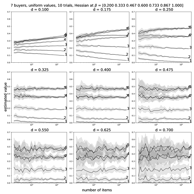
Figure 7: Effect of smoothing parameter on numerical difference estimation of Hessian. Each curve represents the estimated value of ${\mathcal{H}}_{ii}$. Uniform values.

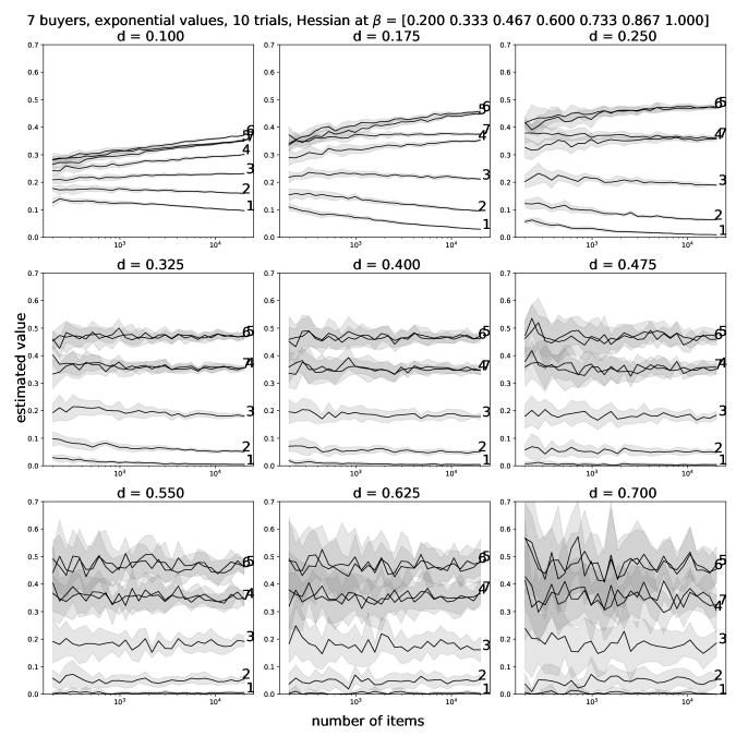
Figure 8: Effect of smoothing parameter on numerical difference estimation of Hessian. Each curve represents the estimated value of ${\mathcal{H}}_{ii}$. Exponential values.

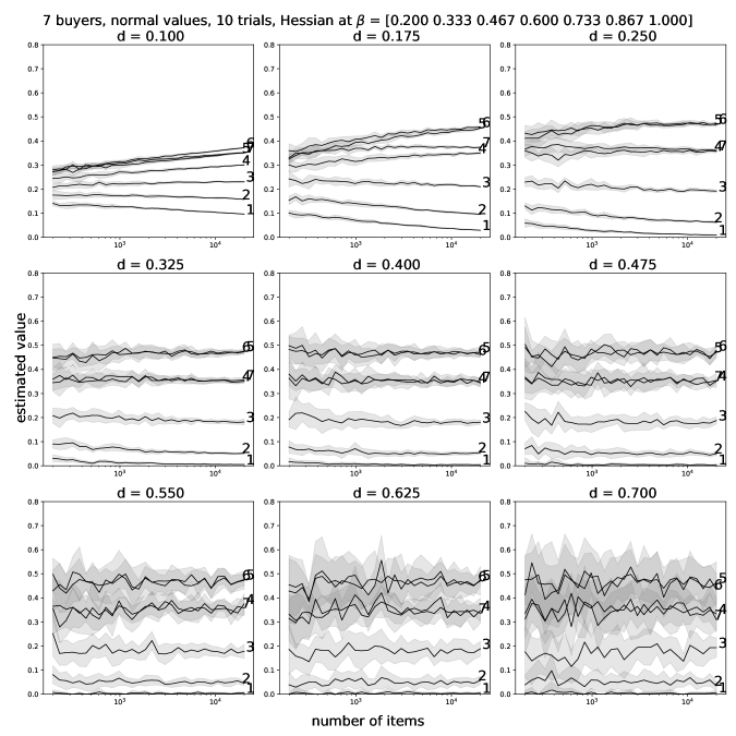
Figure 9: Effect of smoothing parameter on numerical difference estimation of Hessian. Each curve represents the estimated value of ${\mathcal{H}}_{ii}$. Truncated normal values.

14.2 Visualization of FPPE Distribution

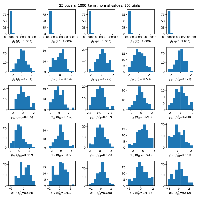
Figure 12: Distribution of $\sqrt{t}({\beta^{\gamma}_{i}-{\beta^{*}_{i}}})$ for all $i\in[n]$. Non-normality and fast convergence for buyers with ${\beta^{*}_{i}}=1$. Truncated normal values.

14.3 Full Version of Table 4

Table 5: Coverage of treatment effect. $\pi$ = treatment probability, the finite difference stepsize $\epsilon_{t}=t^{-0.4}$, proportion of unpaced buyers $\beta_{i}=1$ is 30%

	items	100	200	400	600
buyers	$\pi$
20	0.1	0.8 (5.09)	0.89 (4.96)	0.89 (2.71)	0.92 (1.60)
	0.3	0.91 (3.43)	0.91 (1.74)	0.93 (1.12)	0.92 (0.94)
	0.5	0.91 (3.53)	0.92 (1.47)	0.92 (1.07)	0.92 (0.86)
	0.7	0.92 (3.76)	0.88 (1.96)	0.89 (1.16)	0.9 (0.96)
	0.9	0.79 (3.50)	0.89 (3.57)	0.96 (2.75)	0.91 (2.10)
30	0.1	0.85 (4.20)	0.91 (3.07)	0.9 (25.55)	0.92 (2.98)
	0.3	0.95 (4.26)	0.93 (4.42)	0.94 (1.38)	0.93 (1.03)
	0.5	0.92 (2.80)	0.93 (1.86)	0.92 (1.89)	0.84 (0.97)
	0.7	0.92 (3.91)	0.94 (3.47)	0.91 (1.40)	0.89 (1.09)
	0.9	0.86 (5.09)	0.89 (4.70)	0.92 (2.58)	0.88 (3.15)
40	0.1	0.86 (4.09)	0.91 (3.52)	0.92 (2.00)	0.87 (2.08)
	0.3	0.93 (6.37)	0.94 (4.67)	0.93 (1.26)	0.93 (1.11)
	0.5	0.94 (9.78)	0.9 (2.17)	0.87 (1.21)	0.96 (1.31)
	0.7	0.91 (9.30)	0.96 (6.72)	0.94 (1.73)	0.89 (1.17)
	0.9	0.85 (5.00)	0.85 (5.87)	0.9 (6.01)	0.97 (6.13)
50	0.1	0.88 (8.45)	0.88 (4.75)	0.92 (1.87)	0.88 (1.54)
	0.3	0.95 (3.49)	0.96 (2.37)	0.86 (1.28)	0.93 (1.03)
	0.5	0.92 (3.76)	0.95 (5.05)	0.9 (1.26)	0.94 (0.98)
	0.7	0.85 (3.10)	0.95 (2.27)	0.98 (1.85)	0.95 (1.28)
	0.9	0.76 (3.36)	0.87 (2.87)	0.92 (2.78)	0.96 (9.33)

14.4 Full Version of Table 3

Table 6: Coverage of revenue CI. $\alpha$ = proportion of $\beta_{i}=1$, $d$ is the exponent in finite difference stepsize $\epsilon_{t}=t^{-d}$.

	buyers	20				50				80
	$\alpha$	0.05	0.10	0.20	0.30	0.05	0.10	0.20	0.30	0.05	0.10	0.20	0.30
$d$	items
0.40	100	0.79 (1.72)	0.79 (1.82)	0.93 (1.87)	0.9 (1.81)	0.87 (1.84)	0.81 (1.91)	0.89 (1.82)	0.88 (2.00)	0.81 (1.89)	0.89 (1.89)	0.97 (1.97)	0.9 (1.95)
	200	0.88 (1.33)	0.88 (1.36)	0.87 (1.35)	0.9 (1.34)	0.88 (1.32)	0.93 (1.36)	0.89 (1.37)	0.94 (1.40)	0.87 (1.37)	0.93 (1.37)	0.88 (1.42)	0.86 (1.42)
	400	0.84 (0.93)	0.88 (0.99)	0.93 (0.99)	0.91 (0.98)	0.9 (0.95)	0.94 (0.98)	0.92 (0.98)	0.84 (1.00)	0.88 (0.97)	0.85 (0.98)	0.86 (1.01)	0.85 (1.01)
	600	0.89 (0.76)	0.88 (0.79)	0.9 (0.81)	0.89 (0.80)	0.8 (0.77)	0.87 (0.80)	0.81 (0.80)	0.92 (0.83)	0.86 (0.80)	0.83 (0.80)	0.97 (0.83)	0.89 (0.83)
0.33	100	0.8 (1.75)	0.8 (1.88)	0.9 (1.89)	0.87 (1.87)	0.9 (1.82)	0.88 (1.93)	0.87 (1.84)	0.86 (1.96)	0.88 (1.88)	0.88 (1.90)	0.87 (1.97)	0.93 (1.99)
	200	0.85 (1.29)	0.84 (1.37)	0.91 (1.38)	0.84 (1.38)	0.88 (1.31)	0.93 (1.38)	0.89 (1.38)	0.87 (1.43)	0.89 (1.38)	0.96 (1.37)	0.89 (1.42)	0.9 (1.42)
	400	0.87 (0.93)	0.92 (0.97)	0.91 (0.99)	0.84 (0.98)	0.88 (0.95)	0.93 (0.98)	0.88 (0.97)	0.85 (1.00)	0.95 (0.98)	0.86 (0.96)	0.86 (1.01)	0.86 (1.01)
	600	0.9 (0.76)	0.89 (0.80)	0.84 (0.80)	0.83 (0.80)	0.87 (0.78)	0.87 (0.80)	0.88 (0.81)	0.85 (0.83)	0.9 (0.80)	0.9 (0.80)	0.84 (0.83)	0.89 (0.83)
0.17	100	0.81 (1.80)	0.86 (1.85)	0.89 (1.85)	0.9 (1.87)	0.81 (1.86)	0.84 (1.87)	0.92 (1.91)	0.9 (1.96)	0.93 (1.87)	0.87 (1.85)	0.89 (1.97)	0.92 (1.95)
	200	0.91 (1.30)	0.9 (1.37)	0.88 (1.38)	0.86 (1.37)	0.85 (1.32)	0.87 (1.38)	0.9 (1.36)	0.86 (1.41)	0.9 (1.37)	0.94 (1.38)	0.85 (1.41)	0.9 (1.43)
	400	0.89 (0.93)	0.89 (0.97)	0.89 (0.97)	0.91 (0.98)	0.89 (0.95)	0.88 (0.99)	0.91 (0.97)	0.89 (1.01)	0.96 (0.98)	0.88 (0.97)	0.87 (1.02)	0.9 (1.02)
	600	0.89 (0.76)	0.89 (0.80)	0.84 (0.80)	0.84 (0.80)	0.9 (0.78)	0.89 (0.81)	0.82 (0.80)	0.91 (0.83)	0.89 (0.80)	0.9 (0.81)	0.91 (0.83)	0.89 (0.83)
0.08	100	0.87 (1.80)	0.85 (1.80)	0.87 (1.91)	0.83 (1.87)	0.86 (1.80)	0.95 (1.90)	0.86 (1.89)	0.87 (1.95)	0.89 (1.88)	0.87 (1.86)	0.88 (1.94)	0.89 (1.94)
	200	0.92 (1.30)	0.87 (1.34)	0.9 (1.36)	0.92 (1.35)	0.85 (1.35)	0.88 (1.37)	0.93 (1.36)	0.92 (1.42)	0.87 (1.39)	0.83 (1.36)	0.92 (1.40)	0.91 (1.47)
	400	0.9 (0.93)	0.91 (0.97)	0.93 (0.99)	0.88 (0.97)	0.86 (0.95)	0.91 (0.99)	0.89 (0.98)	0.91 (1.01)	0.9 (0.97)	0.89 (0.97)	0.86 (1.01)	0.89 (1.02)
	600	0.9 (0.76)	0.82 (0.80)	0.93 (0.80)	0.95 (0.81)	0.91 (0.78)	0.88 (0.81)	0.93 (0.81)	0.93 (0.83)	0.92 (0.81)	0.93 (0.80)	0.9 (0.84)	0.88 (0.83)
0.06	100	0.84 (1.79)	0.87 (1.89)	0.85 (1.88)	0.89 (1.81)	0.88 (1.84)	0.93 (1.91)	0.91 (1.88)	0.91 (1.94)	0.91 (1.89)	0.94 (1.91)	0.91 (1.96)	0.87 (2.00)
	200	0.93 (1.30)	0.8 (1.35)	0.92 (1.40)	0.92 (1.35)	0.81 (1.34)	0.89 (1.38)	0.91 (1.34)	0.86 (1.41)	0.91 (1.38)	0.93 (1.39)	0.89 (1.41)	0.91 (1.42)
	400	0.94 (0.93)	0.87 (0.96)	0.8 (0.97)	0.91 (0.97)	0.8 (0.94)	0.93 (1.00)	0.82 (0.97)	0.96 (1.02)	0.9 (0.98)	0.91 (0.99)	0.85 (1.01)	0.91 (1.03)
	600	0.92 (0.76)	0.9 (0.80)	0.88 (0.80)	0.9 (0.80)	0.86 (0.78)	0.92 (0.81)	0.88 (0.80)	0.93 (0.84)	0.88 (0.81)	0.88 (0.80)	0.93 (0.83)	0.93 (0.83)

References

• Aleksandrov et al. (2015) Aleksandrov M, Aziz H, Gaspers S, Walsh T (2015) Online fair division: Analysing a food bank problem. arXiv preprint arXiv:1502.07571 .
• Andrews (1994) Andrews DW (1994) Asymptotics for semiparametric econometric models via stochastic equicontinuity. Econometrica: Journal of the Econometric Society 43–72.
• Andrews (1999) Andrews DW (1999) Estimation when a parameter is on a boundary. Econometrica 67(6):1341–1383.
• Andrews (2001) Andrews DW (2001) Testing when a parameter is on the boundary of the maintained hypothesis. Econometrica 69(3):683–734.
• Aronow and Samii (2017) Aronow PM, Samii C (2017) Estimating average causal effects under general interference, with application to a social network experiment. The Annals of Applied Statistics 11(4):1912–1947.
• Athey et al. (2018) Athey S, Eckles D, Imbens GW (2018) Exact p-values for network interference. Journal of the American Statistical Association 113(521):230–240.
• Athey and Haile (2007) Athey S, Haile PA (2007) Nonparametric approaches to auctions. Handbook of econometrics 6:3847–3965.
• Bajari et al. (2021) Bajari P, Burdick B, Imbens GW, Masoero L, McQueen J, Richardson T, Rosen IM (2021) Multiple randomization designs. arXiv preprint arXiv:2112.13495 .
• Balseiro et al. (2021) Balseiro S, Kim A, Mahdian M, Mirrokni V (2021) Budget-management strategies in repeated auctions. Operations research (3):859–876.
• Balseiro et al. (2015) Balseiro SR, Besbes O, Weintraub GY (2015) Repeated auctions with budgets in ad exchanges: Approximations and design. Management Science 61(4):864–884.
• Balseiro and Gur (2019) Balseiro SR, Gur Y (2019) Learning in repeated auctions with budgets: Regret minimization and equilibrium. Management Science 65(9):3952–3968.
• Bartlett et al. (2005) Bartlett PL, Bousquet O, Mendelson S (2005) Local rademacher complexities. The Annals of Statistics 33(4), ISSN 0090-5364, URL http://dx.doi.org/10.1214/009053605000000282.
• Basse et al. (2016) Basse GW, Soufiani HA, Lambert D (2016) Randomization and the pernicious effects of limited budgets on auction experiments. Artificial Intelligence and Statistics, 1412–1420 (PMLR).
• Bauschke et al. (2011) Bauschke HH, Combettes PL, et al. (2011) Convex analysis and monotone operator theory in Hilbert spaces, volume 408 (Springer).
• Beck (2017) Beck A (2017) First-Order Methods in Optimization, volume 25 (SIAM).
• Bertsekas (1973) Bertsekas DP (1973) Stochastic optimization problems with nondifferentiable cost functionals. Journal of Optimization Theory and Applications 12(2):218–231.
• Blake and Coey (2014) Blake T, Coey D (2014) Why marketplace experimentation is harder than it seems: The role of test-control interference. Proceedings of the fifteenth ACM conference on Economics and computation, 567–582.
• Bojinov and Gupta (2022) Bojinov I, Gupta S (2022) Online experimentation: Benefits, operational and methodological challenges, and scaling guide. Harvard Data Science Review 4(3).
• Bojinov and Shephard (2019) Bojinov I, Shephard N (2019) Time series experiments and causal estimands: exact randomization tests and trading. Journal of the American Statistical Association 114(528):1665–1682.
• Bojinov et al. (2022) Bojinov I, Simchi-Levi D, Zhao J (2022) Design and analysis of switchback experiments. Management Science .
• Borgs et al. (2007) Borgs C, Chayes J, Immorlica N, Jain K, Etesami O, Mahdian M (2007) Dynamics of bid optimization in online advertisement auctions. Proceedings of the 16th international conference on World Wide Web, 531–540.
• Budish (2011) Budish E (2011) The combinatorial assignment problem: Approximate competitive equilibrium from equal incomes. Journal of Political Economy 119(6):1061–1103.
• Budish et al. (2016) Budish E, Cachon GP, Kessler JB, Othman A (2016) Course match: A large-scale implementation of approximate competitive equilibrium from equal incomes for combinatorial allocation. Operations Research 65(2):314–336.
• Cen and Shah (2022) Cen SH, Shah D (2022) Regret, stability & fairness in matching markets with bandit learners. International Conference on Artificial Intelligence and Statistics, 8938–8968 (PMLR).
• Chen et al. (2007) Chen L, Ye Y, Zhang J (2007) A note on equilibrium pricing as convex optimization. International Workshop on Web and Internet Economics, 7–16 (Springer).
• Chen et al. (2023) Chen X, Kroer C, Kumar R (2023) The complexity of pacing for second-price auctions. Mathematics of Operations Research .
• Chen et al. (2003) Chen X, Linton O, Van Keilegom I (2003) Estimation of semiparametric models when the criterion function is not smooth. Econometrica 71(5):1591–1608.
• Clarke (1990) Clarke FH (1990) Optimization and Nonsmooth Analysis (Society for Industrial and Applied Mathematics), URL http://dx.doi.org/10.1137/1.9781611971309.
• Cole et al. (2017) Cole R, Devanur NR, Gkatzelis V, Jain K, Mai T, Vazirani VV, Yazdanbod S (2017) Convex program duality, fisher markets, and Nash social welfare. 18th ACM Conference on Economics and Computation, EC 2017 (Association for Computing Machinery, Inc).
• Conitzer et al. (2022a) Conitzer V, Kroer C, Panigrahi D, Schrijvers O, Stier-Moses NE, Sodomka E, Wilkens CA (2022a) Pacing equilibrium in first price auction markets. Management Science .
• Conitzer et al. (2022b) Conitzer V, Kroer C, Sodomka E, Stier-Moses NE (2022b) Multiplicative pacing equilibria in auction markets. Operations Research 70(2):963–989.
• Dai and Jordan (2021) Dai X, Jordan M (2021) Learning in multi-stage decentralized matching markets. Ranzato M, Beygelzimer A, Dauphin Y, Liang P, Vaughan JW, eds., Advances in Neural Information Processing Systems, volume 34, 12798–12809 (Curran Associates, Inc.), URL https://proceedings.neurips.cc/paper/2021/file/6a571fe98a2ba453e84923b447d79cff-Paper.pdf.
• Devanur et al. (2018) Devanur NR, Garg J, Mehta R, Vaziranb VV, Yazdanbod S (2018) A new class of combinatorial markets with covering constraints: Algorithms and applications. Proceedings of the Twenty-Ninth Annual AC$M$-SIAM Symposium on Discrete Algorithms, 2311–2325 (SIAM).
• Duchi and Ruan (2021) Duchi JC, Ruan F (2021) Asymptotic optimality in stochastic optimization. The Annals of Statistics 49(1):21–48.
• Dupačová (1991) Dupačová J (1991) On non-normal asymptotic behavior of optimal solutions for stochastic programming problems and on related problems of mathematical statistics. Kybernetika 27(1):38–52.
• Dupacová and Wets (1988) Dupacová J, Wets R (1988) Asymptotic behavior of statistical estimators and of optimal solutions of stochastic optimization problems. The annals of statistics 16(4):1517–1549.
• Durrett (2019) Durrett R (2019) Probability: theory and examples, volume 49 (Cambridge university press).
• Eisenberg (1961) Eisenberg E (1961) Aggregation of utility functions. Management Science 7(4):337–350.
• Eisenberg and Gale (1959) Eisenberg E, Gale D (1959) Consensus of subjective probabilities: The pari-mutuel method. The Annals of Mathematical Statistics 30(1):165–168.
• Fradkin (2019) Fradkin A (2019) A simulation approach to designing digital matching platforms. Boston University Questrom School of Business Research Paper Forthcoming .
• Gao and Kroer (2022) Gao Y, Kroer C (2022) Infinite-dimensional fisher markets and tractable fair division. Operation Research .
• Gao et al. (2021) Gao Y, Peysakhovich A, Kroer C (2021) Online market equilibrium with application to fair division. Advances in Neural Information Processing Systems 34:27305–27318.
• Geyer (1994) Geyer CJ (1994) On the asymptotics of constrained $m$-estimation. The Annals of statistics 1993–2010.
• Ghodsi et al. (2011) Ghodsi A, Zaharia M, Hindman B, Konwinski A, Shenker S, Stoica I (2011) Dominant resource fairness: Fair allocation of multiple resource types. Nsdi, volume 11, 24–24.
• Giné and Nickl (2021) Giné E, Nickl R (2021) Mathematical foundations of infinite-dimensional statistical models (Cambridge university press).
• Glynn et al. (2020) Glynn PW, Johari R, Rasouli M (2020) Adaptive experimental design with temporal interference: A maximum likelihood approach. Larochelle H, Ranzato M, Hadsell R, Balcan M, Lin H, eds., Advances in Neural Information Processing Systems, volume 33, 15054–15064 (Curran Associates, Inc.), URL https://proceedings.neurips.cc/paper/2020/file/abd987257ff0eddc2bc6602538cb3c43-Paper.pdf.
• Guo et al. (2021) Guo W, Kandasamy K, Gonzalez JE, Jordan MI, Stoica I (2021) Online learning of competitive equilibria in exchange economies. arXiv preprint arXiv:2106.06616 .
• Hjort and Pollard (2011) Hjort NL, Pollard D (2011) Asymptotics for minimisers of convex processes. arXiv preprint arXiv:1107.3806 .
• Hong and Li (2020) Hong H, Li J (2020) The numerical bootstrap. The Annals of Statistics 48(1):397–412.
• Hsieh et al. (2022) Hsieh YW, Shi X, Shum M (2022) Inference on estimators defined by mathematical programming. Journal of Econometrics 226(2):248–268.
• Hu et al. (2022) Hu Y, Li S, Wager S (2022) Average direct and indirect causal effects under interference. Biometrika .
• Hu and Wager (2022) Hu Y, Wager S (2022) Switchback experiments under geometric mixing. arXiv preprint arXiv:2209.00197 .
• Hudgens and Halloran (2008) Hudgens MG, Halloran ME (2008) Toward causal inference with interference. Journal of the American Statistical Association 103(482):832–842.
• Imbens and Rubin (2015) Imbens GW, Rubin DB (2015) Causal inference in statistics, social, and biomedical sciences (Cambridge University Press).
• Jagadeesan et al. (2021) Jagadeesan M, Wei A, Wang Y, Jordan M, Steinhardt J (2021) Learning equilibria in matching markets from bandit feedback. Advances in Neural Information Processing Systems 34:3323–3335.
• Johari et al. (2022) Johari R, Li H, Liskovich I, Weintraub GY (2022) Experimental design in two-sided platforms: An analysis of bias. Management Science .
• Kash et al. (2014) Kash I, Procaccia AD, Shah N (2014) No agent left behind: Dynamic fair division of multiple resources. Journal of Artificial Intelligence Research 51:579–603.
• Kim and Pollard (1990) Kim J, Pollard D (1990) Cube root asymptotics. The Annals of Statistics 191–219.
• Knight (1999) Knight K (1999) Epi-convergence in distribution and stochastic equi-semicontinuity. Unpublished manuscript 37(7):14.
• Knight (2001) Knight K (2001) Limiting distributions of linear programming estimators. Extremes 4(2):87–103.
• Knight (2006) Knight K (2006) Asymptotic theory for $m$-estimators of boundaries. The Art of Semiparametrics, 1–21 (Springer).
• Knight (2010) Knight K (2010) On the asymptotic distribution of the analytic center estimator. Nonparametrics and Robustness in Modern Statistical Inference and Time Series Analysis: A Festschrift in honor of Professor Jana Jurecková 123.
• Kohavi and Thomke (2017) Kohavi R, Thomke S (2017) The surprising power of online experiments. Harvard business review 95(5):74–82.
• Kosorok (2008) Kosorok MR (2008) Introduction to empirical processes and semiparametric inference. (Springer).
• Kroer et al. (2023a) Kroer C, Sinha D, Zhang X, Cheng S, Zhou Z (2023a) Fair notification optimization: An auction approach. arXiv preprint arXiv:2302.04835 .
• Kroer et al. (2023b) Kroer C, Sinha D, Zhang X, Cheng S, Zhou Z (2023b) Fair notification optimization: An auction approach. URL http://dx.doi.org/10.3886/K3QX-XZ33.
• Kroer and Stier-Moses (2022) Kroer C, Stier-Moses NE (2022) Market equilibrium models in large-scale internet markets. Innovative Technology at the Interface of Finance and Operations. Springer Series in Supply Chain Management. Springer Natures, Forthcoming .
• Larsen et al. (2022) Larsen N, Stallrich J, Sengupta S, Deng A, Kohavi R, Stevens N (2022) Statistical challenges in online controlled experiments: A review of a/b testing methodology. arXiv preprint arXiv:2212.11366 .
• Le Cam et al. (2000) Le Cam L, LeCam LM, Yang GL (2000) Asymptotics in statistics: some basic concepts (Springer Science & Business Media).
• Leung (2020) Leung MP (2020) Treatment and spillover effects under network interference. Review of Economics and Statistics 102(2):368–380.
• Li et al. (2022) Li H, Zhao G, Johari R, Weintraub GY (2022) Interference, bias, and variance in two-sided marketplace experimentation: Guidance for platforms. Proceedings of the ACM Web Conference 2022, 182–192.
• Li (2022) Li J (2022) The proximal bootstrap for constrained estimators .
• Li and Wager (2022) Li S, Wager S (2022) Random graph asymptotics for treatment effect estimation under network interference. The Annals of Statistics 50(4):2334–2358.
• Liao et al. (2014) Liao H, Peng L, Liu Z, Shen X (2014) ipinyou global rtb bidding algorithm competition dataset. Proceedings of the Eighth International Workshop on Data Mining for Online Advertising, 1–6.
• Liao et al. (2022) Liao L, Gao Y, Kroer C (2022) Nonstationary dual averaging and online fair allocation. Advances in Neural Information Processing Systems 35:37159–37172.
• Liao et al. (2023) Liao L, Gao Y, Kroer C (2023) Statistical inference for fisher market equilibrium. International Conference on Learning Representations.
• Liao and Kroer (2023) Liao L, Kroer C (2023) Statistical Inference and A/B Testing for First-Price Pacing Equilibria. International Conference on Machine Learning.
• Liao and Kroer (2024) Liao L, Kroer C (2024) Bootstrapping fisher market equilibrium and first-price pacing equilibrium.
• Liu et al. (2009) Liu H, Lafferty J, Wasserman L (2009) The nonparanormal: Semiparametric estimation of high dimensional undirected graphs. Journal of Machine Learning Research 10(10).
• Liu et al. (2021a) Liu LT, Ruan F, Mania H, Jordan MI (2021a) Bandit learning in decentralized matching markets. J. Mach. Learn. Res. 22:211–1.
• Liu et al. (2021b) Liu M, Mao J, Kang K (2021b) Trustworthy and powerful online marketplace experimentation with budget-split design. Proceedings of the 27th ACM SIGKDD Conference on Knowledge Discovery & Data Mining, 3319–3329.
• Liu et al. (2022) Liu Z, Lu M, Wang Z, Jordan M, Yang Z (2022) Welfare maximization in competitive equilibrium: Reinforcement learning for markov exchange economy. International Conference on Machine Learning, 13870–13911 (PMLR).
• McElfresh et al. (2023) McElfresh DC, Kroer C, Pupyrev S, Sodomka E, Sankararaman K, Chauvin Z, Dexter N, Dickerson JP (2023) Matching algorithms for blood donation. Nature Machine Intelligence 5(10):1108–1118, ISSN 2522-5839, URL http://dx.doi.org/10.1038/s42256-023-00722-5.
• Min et al. (2022) Min Y, Wang T, Xu R, Wang Z, Jordan MI, Yang Z (2022) Learn to match with no regret: Reinforcement learning in markov matching markets. arXiv preprint arXiv:2203.03684 .
• Munro et al. (2023) Munro E, Wager S, Xu K (2023) Treatment effects in market equilibrium. arXiv preprint arXiv:2109.11647 .
• Newey and McFadden (1994) Newey WK, McFadden D (1994) Large sample estimation and hypothesis testing. Handbook of econometrics 4:2111–2245.
• Nisan et al. (2007) Nisan N, Roughgarden T, Tardos E, Vazirani VV (2007) Algorithmic game theory (Cambridge University Press).
• Othman et al. (2010) Othman A, Sandholm T, Budish E (2010) Finding approximate competitive equilibria: efficient and fair course allocation. AAMAS, volume 10, 873–880.
• Pakes and Pollard (1989) Pakes A, Pollard D (1989) Simulation and the asymptotics of optimization estimators. Econometrica: Journal of the Econometric Society 1027–1057.
• Parkes et al. (2015) Parkes DC, Procaccia AD, Shah N (2015) Beyond dominant resource fairness: Extensions, limitations, and indivisibilities. ACM Transactions on Economics and Computation (TEAC) 3(1):1–22.
• Rockafellar (1970) Rockafellar RT (1970) Convex analysis, volume 18 (Princeton university press).
• Rockafellar and Wets (2009) Rockafellar RT, Wets RJB (2009) Variational analysis, volume 317 (Springer Science & Business Media).
• Sahoo and Wager (2022) Sahoo R, Wager S (2022) Policy learning with competing agents. arXiv preprint arXiv:2204.01884 .
• Self and Liang (1987) Self SG, Liang KY (1987) Asymptotic properties of maximum likelihood estimators and likelihood ratio tests under nonstandard conditions. Journal of the American Statistical Association 82(398):605–610.
• Shapiro (1988) Shapiro A (1988) Sensitivity analysis of nonlinear programs and differentiability properties of metric projections. SIAM Journal on Control and Optimization 26(3):628–645.
• Shapiro (1989) Shapiro A (1989) Asymptotic properties of statistical estimators in stochastic programming. The Annals of Statistics 17(2):841–858.
• Shapiro (1990) Shapiro A (1990) On differential stability in stochastic programming. Mathematical Programming 47(1):107–116.
• Shapiro (1991) Shapiro A (1991) Asymptotic analysis of stochastic programs. Annals of Operations Research 30(1):169–186.
• Shapiro (1993) Shapiro A (1993) Asymptotic behavior of optimal solutions in stochastic programming. Mathematics of Operations Research 18(4):829–845.
• Shapiro (2000) Shapiro A (2000) On the asymptotics of constrained local $m$-estimators. Annals of statistics 948–960.
• Shapiro (2003) Shapiro A (2003) Monte carlo sampling methods. Handbooks in operations research and management science 10:353–425.
• Shapiro et al. (2021) Shapiro A, Dentcheva D, Ruszczynski A (2021) Lectures on stochastic programming: modeling and theory (SIAM).
• Sinclair et al. (2022) Sinclair SR, Banerjee S, Yu CL (2022) Sequential fair allocation: Achieving the optimal envy-efficiency tradeoff curve. Abstracts of the 2022 SIGMETRICS/Performance Joint International Conference on Measurement and Modeling of Computer Systems.
• Sneider et al. (2018) Sneider C, Tang Y, Tang Y (2018) Experiment rigor for switchback experiment analysis. URL: https://doordash. engineering/2019/02/20/experiment-rigor-for-switchback-experiment-analysis .
• Vaart and Wellner (1996) Vaart AW, Wellner JA (1996) Weak convergence. Weak convergence and empirical processes, 16–28 (Springer).
• Van der Vaart (2000) Van der Vaart AW (2000) Asymptotic statistics, volume 3 (Cambridge university press).
• Varian (1974) Varian HR (1974) Equity, envy, and efficiency. Journal of Economic Theory 9(1):63–91.
• Wager and Xu (2021) Wager S, Xu K (2021) Experimenting in equilibrium. Management Science 67(11):6694–6715, URL http://dx.doi.org/10.1287/mnsc.2020.3844.
• Wainwright (2019) Wainwright MJ (2019) High-dimensional statistics: A non-asymptotic viewpoint, volume 48 (Cambridge University Press).
• Wang (1985) Wang J (1985) Distribution sensitivity analysis for stochastic programs with complete recourse. Mathematical Programming 31(3):286–297.
• Xiao (2010) Xiao L (2010) Dual averaging methods for regularized stochastic learning and online optimization. Journal of Machine Learning Research 11:2543–2596.
• Zhao and Udell (2020) Zhao Y, Udell M (2020) Missing value imputation for mixed data via gaussian copula. Proceedings of the 26th ACM SIGKDD international conference on knowledge discovery & data mining, 636–646.
\ECSwitch
{APPENDICES}
\ECHead