The next galactic supernova can uncover mass and couplings of particles decaying to neutrinos

Abstract

Many particles predicted by extensions of the Standard Model feature interactions with neutrinos, e.g., Majoron-like bosons $\phi$. If the mass of $\phi$ is larger than about $10\,\rm keV$, they can be produced abundantly in the core of the next galactic core-collapse supernova through neutrino coalescence, and leave it with energies of around 100 MeV. Their subsequent decay to high-energy neutrinos and anti-neutrinos provides a distinctive signature at Earth. Ongoing and planned neutrino and dark matter experiments allow us to reconstruct the energy, flavor, and time of arrival of these high-energy neutrinos. For the first time, we show that these measurements can help pinpointing the mass of $\phi$ and its couplings to neutrinos of different flavor. Our results can be generalized in a straightforward manner to other hypothetical feebly interacting particles, like novel gauge bosons or heavy neutral leptons, that decay into neutrinos.

1 Introduction

Because neutrinos interact weakly with other particles of the Standard Model (SM), their properties are the least understood, making them compelling candidates to act as portals to new physics [1, 2, 3]. Many proposed extensions of the SM posit new particles that couple to neutrinos, including new neutral leptons [4, 5], bosons associated with novel gauge symmetries [6, 7, 8, 9], and Goldstone and pseudo-Goldstone bosons associated with the spontaneous breaking of global symmetries [10, 11, 12, 13]. The search for physics beyond the SM (BSM) through neutrinos spans astrophysical, cosmological, and laboratory observations; for a necessarily limited list, see Refs. [14, 15, 16, 17, 18, 19, 20, 21, 22, 23, 24, 25, 26, 27, 28, 29, 30, 31, 32, 33, 34, 35, 36, 37, 38, 39, 40, 41, 42, 43, 44, 45, 46, 47, 48, 49].

Together with the early universe, the hot, dense cores of collapsing stars are the only places where neutrinos can reach thermal equilibrium. At such large temperatures and densities, supernovae (SNe) might be powerful factories of new particles that couple to neutrinos. These include Majoron-like bosons, $\phi$, hereafter simply called Majorons, whose interaction with neutrinos is of the form (see, e.g., Ref. [25])

$$\mathcal{L}_{\text{int}}=-\sum_{\alpha}\frac{g_{\alpha}}{2}\,\psi_{\alpha}^{T}\sigma_{2}\psi_{\alpha}\phi+\textrm{h.c.}\;,$$ (1.1)

where $\psi_{\alpha}$ is the two-component Majorana neutrino field with flavor $\alpha=e,\mu,\tau$, and $g_{\alpha}$ is the coupling, which must be a real number. For simplicity, we restrict ourselves to the case of flavor-diagonal couplings. The above coupling entails lepton number violation.

If Majorons have a mass $m_{\phi}\gtrsim 10\,\rm keV$, they could be produced abundantly in the cores of SNe through neutrino coalescence, $\nu\nu\to\phi$. These Majorons can leave the core with energies of hundreds of MeV, take energy away from the core, and shorten the duration of the standard neutrino signal expected at neutrino detectors. As a result, one can infer neutrino cooling bounds on $\phi$—akin to those on the QCD axion [50, 51, 52, 53], axion-like particles [54, 55, 56, 57, 58, 59], dark photons [60, 61], or millicharged particles [62, 63]—by looking at the time distribution of the SN 1987A neutrinos detected by Kamiokande II [64, 65, 66, 67, 68], the Irvine–Michigan–Brookhaven [69, 70, 71], and the Baksan Underground Scintillation Telescope (BUST) [72, 73]. However, it was pointed out in Ref. [43] that $\phi$ could have decayed back to neutrinos away from the cooling proto-neutron star, producing a flux of neutrinos with unexpectedly high energies compared to the standard tens-of-MeV neutrinos emitted from the neutrinosphere. Since such flux was not observed from SN 1987A, one can draw constraints which are always stronger than the cooling bounds. (See also Ref. [74] for an application to a list of models.)

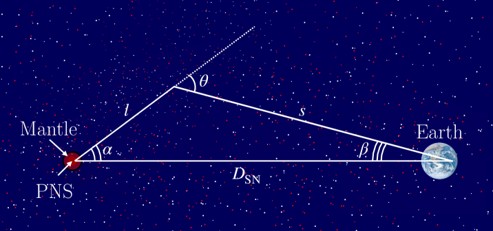
Figure 1: Difference between the time of arrival of neutrinos sourced by the neutrinosphere and by Majoron decay. The length travelled by a neutrino emitted by the PNS surface is $D_{\rm SN}$, while a neutrino produced through Majoron decay accumulates a delay. The resulting time spread of the signal depends on the Majoron coupling to neutrinos, $g$, but not on the Majoron mass, $m_{\phi}$ (see Appendix A); figure is not to scale, since for our parameter space $l\ll D_{\rm SN}$. Combining timing and energy information one can obtain the mass and coupling of the Majoron to neutrinos.

As observed in Ref. [75], the next galactic core-collapse SN constitutes a preferred target for future searches of novel particles that couple to neutrinos. Upcoming neutrino detectors will be orders-of-magnitude larger than present ones, and the latest large dark-matter detectors will also be able to observe neutrinos from SNe. In this paper, we revisit the discovery reach of Majorons by combining new detectors and showing how the results depend on the assumed SN model. Crucially, we show that combining all the information on the time-dependent (rather than the time-integrated) neutrino flux at Earth, i.e., energy, flavor, and time of arrival of the neutrinos, we might be able to partially reconstruct the couplings and mass of $\phi$. First, the flavor information, which can be uncovered from the different event topologies in the detector, can be directly connected with the individual flavor couplings $g_{\alpha}$. Second, although the time-integrated flux depends on the combination $g_{\alpha}m_{\phi}$, the high-energy neutrinos produced by Majoron decays would arrive spread in time with respect to the standard SN neutrinos (see Fig. 1), with the width of the spread depending on the couplings only, thus breaking the degeneracy between couplings and mass. While we obtain our results explicitly for the simple interaction Lagrangian of Eq. (1.1), mutatis mutandis one can generalize our findings to any BSM scenario featuring a particle light enough to be produced by SNe and that can decay to neutrinos.

2 Neutrinos from Majoron decay

In the SN core, neutrinos and anti-neutrinos have thermal potentials of equal size but opposite signs, dominated by neutrons, with absolute value $|V|=G_{\rm F}\rho/\sqrt{2}m_{N}\sim 10$ eV, where $m_{N}$ is the nucleon mass, for a typical nuclear density $\rho\sim 3\times 10^{14}$ g cm^-3. For a typical neutrino energy $E_{\nu}\sim 100$ MeV, if the Majoron mass $m_{\phi}\gtrsim\sqrt{|V|E_{\nu}}\sim 10$ keV, the dominant Majoron production channel is the coalescence of pairs of neutrinos, $\nu_{\alpha}+\nu_{\alpha}\to\phi$, and anti-neutrinos, $\bar{\nu}_{\alpha}+\bar{\nu}_{\alpha}\to\phi$. Summing over neutrinos and anti-neutrinos of all flavors ($\alpha=e,\mu,\tau$), the resulting energy spectrum of emitted Majorons of energy $E_{\phi}$, per unit volume and time, is [43]

$$\frac{d\dot{n}_{\phi}}{dE_{\phi}}=\sum_{\sigma=\pm}\sum_{\alpha}\frac{g_{\alpha}^{2}m_{\phi}^{2}}{64\pi^{3}}\int_{E_{-}}^{E_{+}}\!\!dE_{\nu}\,f^{\sigma}_{\alpha}(E_{\nu})f^{\sigma}_{\alpha}(E_{\phi}-E_{\nu})\;,$$ (2.1)

where $f^{\sigma}_{\alpha}(E_{\nu})=\bigl{[}e^{(E_{\nu}-\sigma\mu_{\alpha})/T}+1\bigr{]}^{-1}$ is the Fermi-Dirac distribution of $\nu_{\alpha}$ (for $\sigma=+1$) or $\bar{\nu}_{\alpha}$ (for $\sigma=-1$), which are in local thermal equilibrium with temperature $T$ and have chemical potential $\sigma\mu_{\alpha}$, $E_{\pm}\equiv\frac{1}{2}(E_{\phi}\pm p_{\phi})$, and $p_{\phi}=\sqrt{E_{\phi}^{2}-m_{\phi}^{2}}$ is the momentum of the Majoron. Local thermal equilibrium holds throughout the proto-neutron star (PNS), where the bulk of the Majoron emission occurs. Because inside the PNS electron neutrinos are degenerate, with a chemical potential of $\mu_{e}\sim 100$ MeV, they dominate the Majoron production and thus the typical energy of the Majorons is comparable, i.e., $E_{\phi}\sim\mu_{e}$.

The total number of Majorons produced throughout the SN evolution is

$$\frac{dN_{\phi}}{dE_{\phi}}=\int\frac{d\dot{n}_{\phi}}{dE_{\phi}}dVdt\;,$$ (2.2)

where the integral is over the spatial and temporal profiles of a supernova simulation. We use two one-dimensional supernova models, SFHo-18.8 and LS220-s20.0, that were evolved using the Prometheus Vertex code with six-species neutrino transport [76]. They represent, respectively, the case of a very heavy (final neutron star baryonic mass of $1.926\;M_{\odot}$, where $M_{\odot}$ is one solar mass) and a very light PNS (final neutron star baryonic mass of $1.351\;M_{\odot}$). The profiles of temperature and chemical potential for both models are shown in the Supplemental Material of Ref. [43]. Following Refs. [54, 56, 43, 63], we dub them the hot and cold models, respectively, as they present comparably high (up to $60$ MeV) and low temperatures (up to $40$ MeV). We extract the chemical potentials for $\nu_{e}$ and $\nu_{\mu}$ from the simulations. For $\nu_{\tau}$, for which the chemical potential is not available, we consider zero chemical potential. In reality, for the latter, a small chemical potential does build up, because $\overline{\nu}_{\tau}$ interact less with nucleons than $\nu_{\tau}$ due to weak-magnetism corrections to the cross sections [77], but remains significantly smaller than for the other neutrino species.

The Majoron energy emission is in general time-dependent. Its time structure, which is shown in the Supplemental Material of Ref. [43], peaks immediately after the bounce, since it is correlated with the large chemical potential of neutrinos. However, for our analyses we always consider the time-integrated emission of Majorons, Eq. (2.2).

After Majorons are emitted, they decay via $\phi\to\nu_{\alpha}+\nu_{\alpha}$ at a rest-frame rate of

$$\Gamma_{\phi\to\nu\nu}=\sum_{\alpha}\frac{g_{\alpha}^{2}m_{\phi}}{32\pi}\;,$$ (2.3)

and at an identical rate via $\phi\to\bar{\nu}_{\alpha}+\bar{\nu}_{\alpha}$; hence, their total decay rate is $2\Gamma_{\phi\to\nu\nu}$. In the laboratory frame, the Majoron lifetime is lengthened by a factor $E_{\phi}/m_{\phi}$ due to time dilation. Nevertheless, for the ranges of couplings and masses that we consider, the Majorons decay long before reaching Earth. Even for a coupling of $gm_{\phi}\sim 10^{-11}$ MeV, the decay length of a Majoron with energy $E_{\phi}\sim 100$ MeV is about $10^{-3}$ pc, tiny compared to the 10-kpc-scale distances to the SN that we consider. The daughter neutrinos have energies comparable to the parent Majoron, i.e., in the $100$-MeV range, significantly higher than standard SN neutrinos (Section 3), whose energies are in the 10-MeV range. Thus, the detection of high-energy neutrinos at Earth would provide an identifying signature of Majorons.

Majorons decay into $\nu_{\alpha}$ or $\bar{\nu}_{\alpha}$ with branching ratios $\mathrm{Br}(\phi\to\nu_{\alpha}+\nu_{\alpha})=\mathrm{Br}(\phi\to\bar{\nu}_{\alpha}+\bar{\nu}_{\alpha})=g_{\alpha}^{2}/(2\sum_{\beta}g_{\beta}^{2})$; the factor of $2$ accounts for the decay in neutrinos and anti-neutrinos evenly. As neutrinos propagate, they mix; upon reaching Earth, the fraction of $\nu_{\alpha}$ in the total flux is $f_{\alpha}=\sum_{i=1,2,3}\sum_{\beta=e,\mu,\tau}|U_{\alpha i}|^{2}|U_{\beta i}|^{2}\mathrm{Br}(\phi\to\nu_{\beta}+\nu_{\beta})$, where $U$ is the Pontecorvo-Maki-Nakagawa-Sakata (PMNS) matrix. The energy spectrum of the daughter neutrinos from the decay of Majorons has a characteristic box shape flat in neutrino energy, so the energy fluence of $\nu_{\alpha}$ at Earth is

$$\frac{d\mathcal{F}_{\alpha}}{dE_{\nu}}=\frac{2f_{\alpha}}{4\pi D_{\mathrm{SN}}^{2}}\int_{E_{\rm min}}^{\infty}\frac{dE_{\phi}}{p_{\phi}}\frac{dN_{\phi}}{dE_{\phi}}\Big{|}_{E_{\phi}}\;,$$ (2.4)

and identically for $\overline{\nu}_{\alpha}$, where $D_{\mathrm{SN}}$ is the SN distance from Earth; the factor $2$ accounts for the two daughter neutrinos produced in each decay. We use $D_{\mathrm{SN}}=10$ kpc as a reference value, corresponding roughly to a SN occurring at the galactic center. The minimum Majoron energy needed to produce a neutrino of energy $E_{\nu}$ is $E_{\rm min}=E_{\nu}+m_{\phi}^{2}/(4E_{\nu})$. Setting $f_{\alpha}=1/6$ in Eq. (2.4) reproduces the analogous result of Ref. [43]. The spectrum of the neutrinos emitted from the Majoron decay is shown in Fig. 2 of Ref. [43].

For sufficiently small couplings, $g_{\alpha}$, and large masses, $m_{\phi}$, the Majorons would be significantly slowed down compared to the standard neutrinos. The typical time scale after which a Majoron decays is roughly $\tau_{\phi}\sim E_{\phi}/(\Gamma_{\phi\to\nu\nu}m_{\phi})\sim E_{\phi}/\sum_{\alpha}g_{\alpha}^{2}m_{\phi}^{2}$. Within this time scale, the Majoron accumulates a delay due to its velocity, $v_{\phi}=\sqrt{1-m_{\phi}^{2}/E_{\phi}^{2}}$, of about $\tau_{\phi}(1-v_{\phi})\sim 1/\sum_{\alpha}g_{\alpha}^{2}E_{\phi}$. The daughter neutrinos are produced at a typical angle $\theta\sim m_{\phi}^{2}/E_{\phi}^{2}$ with respect to the direction of the Majoron, so this angular deflection produces a comparable delay. The net result is that the neutrino emission from Majoron decay is not delayed relative to the emission of standard neutrinos, since some of the Majorons decay early, but rather stretched over a time scale of about $\tau_{\phi}(1-v_{\phi})$, which is independent of the Majoron mass, as it would be for any BSM model with an operator of dimension 4. We account for the above effects by computing the time-dependent neutrino energy spectrum at Earth as

$$\frac{d\Phi_{\alpha}(t)}{dE_{\nu}}=\frac{d\mathcal{F}_{\alpha}}{dE_{\nu}}\exp\left[-\frac{2\Gamma_{\phi}E_{\nu}t}{m_{\phi}}\right]\frac{2\Gamma_{\phi}E_{\nu}}{m_{\phi}}\;.$$ (2.5)

In Eq. (2.5), while the spectrum of daughter neutrinos, $d\mathcal{F}_{\alpha}/dE_{\nu}$, depends on the Majoron couplings and mass—roughly $\propto g_{\alpha}m_{\phi}$, for low values of $m_{\phi}$—the terms introduced by the stretching of their emission time depend only on the coupling. In our time-dependent analysis (Section 5.2) this will break the degeneracy between coupling and mass. We review the derivation of Eq. (2.5) in Appendix A; see also, e.g., Ref. [78].

3 Standard supernova neutrinos

The vast majority of the neutrinos from the next galactic core-collapse SN will be made in SM processes. For the purpose of our work, they act as background to our search for the neutrinos made in the decay of Majorons. Here we review the main properties of the standard SN neutrino flux and discuss how we model it. For a more detailed discussion of SN neutrino emission, we refer to dedicated reviews, e.g., Ref. [79].

The SN explosion is triggered by the collapse of the core of a very massive star. When the core reaches nuclear densities, the collapse is suddenly halted and a shock wave is launched towards the outer stellar layers. Neutrinos in the inner regions are kept in thermal and chemical equilibrium by weak interactions with the surrounding nuclear matter, with $\nu_{e}$ being highly degenerate due to the relatively large lepton number trapped in the SN core. The region where neutrinos remain in equilibrium with matter is approximately bounded by a neutrinosphere, beyond which the neutrino interaction rate with matter drops sufficiently for neutrinos to escape; this happens typically at a distance of about $20$ km from the center of the core. In reality, the concept of neutrinosphere is a fuzzy one, and different species decouple at different distances, but it provides a qualitative grasp on the distances involved.

At the earliest stage of the SN, neutrino emission is due to the shock breakout from the neutrinosphere, leading to a burst—the neutronization burst—of $\nu_{e}$ produced in the neutronization of free protons $p+e^{-}\to n+\nu_{e}$ in the core. This burst has a high instantaneous luminosity, of the order of $10^{53}$ erg s^-1, but it is short, lasting only about 50 ms. In our analysis, we do not consider neutrinos from the neutronization burst. Rather, our focus is on the longer-duration neutrino emission of later SN stages, and on the high-energy neutrinos created in the decays of Majorons, altogether spanning tens of seconds.

After the shock breakout, the matter behind the shock starts to accrete onto the surface of the PNS, powering neutrino emission. During this accretion phase, lasting 0.5–1 s, the shock wave remains essentially stalled. The PNS undergoes sustained neutrino emission with typical luminosities of $10^{52}$ erg s^-1. In the neutrino delayed shock mechanism, a fraction of this energy is deposited below the shock wave, reviving it and leading to the SN explosion. Afterwards, the PNS undergoes a cooling phase, where neutrinos are emitted with a quasi-thermal spectrum, for a typical duration of $5$–$6\,\rm s$. At later times, additional emission might come from fallback accretion of material, an intrinsically three-dimensional process which is known with less certainty than the previous phases.

The total energy of the emitted neutrinos, $E_{\rm tot}$, is roughly $10^{53}$ erg, and has a marked dependence on the mass of the PNS, with heavier PNSs yielding higher neutrino luminosities; the equation of state can also impact the neutrino emission. The average energy of the emitted neutrinos, $E_{0}$, is typically 12–14 MeV. Following Refs. [80, 81, 82], we model the time-integrated (excluding the neutronization burst), all-species energy spectrum of the emitted neutrinos as

$$\frac{dN_{\nu}}{dE_{\nu}}=\frac{E_{\mathrm{tot}}}{E_{0}^{2}}\frac{(1+\alpha)^{1+\alpha}}{\Gamma(1+\alpha)}\left(\frac{E_{\nu}}{E_{0}}\right)^{\alpha}e^{-(1+\alpha)E_{\nu}/E_{0}}\;,$$ (3.1)

where $\Gamma$ is the Gamma function and $\alpha$ is the pinch parameter; $\alpha=2$ corresponds to a Maxwell-Boltzmann spectrum. The emitted spectra are different for the different species, with $\nu_{e}$ having lower energies than the other ones due to their higher interaction rate, which keeps them in equilibrium with nuclear matter at larger radii with lower temperatures. However, the differences are generally small, with the average energy of $\nu_{e}$ typically around $9$ MeV and of the other species typically around $12$ MeV. The total emitted energy for different species is quite similar, with up to $\sim 5\%$ differences (see, e.g., Table VII of Ref. [83]). We ignore these small differences and assume a common shape, Eq. (3.1), for the spectrum of all neutrino species. For the two SN models that we consider, we use the values of the parameters in Eq. (3.1) from Ref. [43]: in the cold model, $E_{\rm tot}=1.98\times 10^{53}$ erg, $E_{0}=12.7$ MeV, and $\alpha=2.39$; in the hot model, $E_{\rm tot}=3.93\times 10^{53}$ erg, $E_{0}=14.3$ MeV, and $\alpha=2.07$.

The flavor composition of the neutrino flux detected at Earth, i.e., the proportion of $\nu_{e}$, $\nu_{\mu}$, and $\nu_{\tau}$ in it, is affected by neutrino mixing and its interplay with weak interactions. In the regions close to the neutrinosphere, weak interactions can induce fast flavor conversions [84, 85, 86, 87, 88, 89, 90, 91] where neutrinos traveling along different directions change flavor via the refractive forward scattering $\bar{\nu}_{e}+\nu_{e}\to\bar{\nu}_{\mu}+\nu_{\mu}$. Although the kinetic equations describing fast flavor conversions are well-known [92, 93, 94, 95, 96, 97, 98, 99, 100, 101, 102], their outcome and impact on supernova evolution largely is not; see, e.g., Refs. [89, 103] and references therein. The typical length scale over which flavor would change is of the order of cm, much shorter compared to the hydrodynamical scale, making a direct numerical implementation of both scales a formidable problem beyond current computational capabilities. When the dynamics is entirely driven by the refractive exchange, numerical [104] and theoretical [105] arguments suggest that flavor equipartition is reached along certain directions, but the interplay between the refractive exchange and neutrino collisions with matter remains an open question [106, 107, 108, 109, 110, 111, 112, 113, 114, 115, 116]. In any case, the feedback of the altered neutrino flavor composition on the hydrodynamical simulations has not been self-consistently studied, although it appears that if large changes occur there could be considerable impact on the supernova evolution [117, 118].

In the outer regions of the SN, where the neutrino density is lower, the interplay between neutrino mixing in vacuum and refractive flavor exchange could still induce slow flavor conversions, which could give rise to energy-dependent flavor swaps [119, 120, 121]. In addition, standard Mikheyev–Smirnov–Wolfenstein (MSW) resonances [122, 123] in neutrino-matter interactions would affect neutrino mixing, but their precise effect depends on the unknown degree of adiabaticity of the matter density profile and the ordering of the neutrino mass eigenstates, and thus remains unclear; for details, see Refs. [124, 103] and references therein. In any case, predictions of these behaviors in the outer regions are unavoidably conditioned by the lack of understanding of fast conversions.

In view of the above uncertainties, we restrict ourselves to the simplest assumption of species equipartition in the standard SN neutrino flux at Earth, i.e., that the flux is evenly divided among $\nu_{e}$, $\bar{\nu}_{e}$, $\nu_{\mu}$, $\bar{\nu}_{\mu}$, $\nu_{\tau}$, and $\bar{\nu}_{\tau}$ but point out that this should be revisited later, once flavor conversions inside SNe are better understood. These uncertainties do not affect Majoron emission, which happens in the core, where neutrinos are in chemical equilibrium with the surrounding matter and neutrino mixing is inhibited.

As pointed out above, the standard neutrino flux acts as a background to our search for the high-energy neutrinos from Majoron decays. Since the abundance of the latter peaks in the $100$-MeV range, there is a clear separation between the two neutrino signals, and our sensitivity to neutrinos from Majoron decays comes mainly from these high energies. This fact renders the impact of how we model the standard SN signal on our results largely unimportant. In the energy window between 30–70 MeV, the overlap between the standard and non-standard SN components does require that the two are disentangled. Hence, we model the time-integrated SN neutrino fluence with the spectrum from Eq. (3.1), assuming, as mentioned above, equipartition among different species. Relieving these analysis choices would enlarge the model parameter space of our analysis without adding any new qualitative feature to it, nor affecting our results sizably, since they rest rather on the starkly different energy scales of the standard and non-standard neutrino fluxes.

We only model the time-integrated neutrino fluence. In principle, for a time-dependent analysis like the one we perform later (Section 5), it would be helpful to also disentangle the standard neutrino flux from the flux of neutrinos from Majoron decays by using some parametrization of the time-dependent standard flux. However, no such parametrization presently exists. A first attempt in this direction has only recently been performed in Ref. [125]; however, it is only for the time dependence of the energy-integrated neutrino luminosity, not for the energy spectrum. Thus, when we do turn to a time-dependent analysis, we choose conservatively to simply remove the low-energy events in order to eliminate the SN neutrino flux rather than model it, as we discuss in detail in Section 5.

4 Neutrino detection from the next galactic supernova

The next galactic supernova will lead to the detection of a very large signal at a host of different observatories. Here, we are mainly interested in the possibility that a small fraction of high-energy events might be observed, which would be a smoking-gun signature of novel bosons produced in the SN core such as the Majoron we study here. If these events were to be observed, we aim to understand to what degree they could be used to reconstruct the properties of the novel bosons. Below, we review the main detection channels of SN neutrinos and estimate their expected detection rate.

4.1 Neutrino detection processes

All of the neutrino detection processes entail the scattering of a neutrino or an anti-neutrino off a nucleus, a nucleon, or an electron. We list below the main processes.

4.1.1   Quasi-elastic (QE) electron neutrino scattering

In water Cherenkov detectors, $\overline{\nu}_{e}$ can be detected via inverse beta decay (IBD) on free protons, $\bar{\nu}_{e}+p\to n+e^{+}$, and both $\nu_{e}$ and $\overline{\nu}_{e}$ through their charged-current scattering on oxygen nuclei, $\nu_{e}+\ce{{}^{1}6O}\to e^{-}+X$ and $\bar{\nu}_{e}+\ce{{}^{1}6O}\to e^{+}+Y$, where $X$ and $Y$ denote final excited nuclear states. For $\bar{\nu}_{e}$, the latter reactions dominate over IBD at neutrino energies larger than about 70 MeV. Above the kinematic threshold, the cross section for QE neutrino–nucleus ($\nu A$) scattering grows as $\sigma_{\nu_{e}A}\propto E_{\nu}^{2}$. Therefore, a high-energy neutrino from Majoron decay is more likely to be detected than a lower-energy standard SN neutrino. We neglect the recoil energy of the nucleus, so that the energy of the final-state electron is simply $E_{e}=E_{\nu}-Q_{\nu_{e}A}$, and $E_{e}=E_{\nu}-Q_{\bar{\nu}_{e}A}$ for the positron, where the transferred momentum, $Q_{\nu_{e}A}$ or $Q_{\bar{\nu}_{e}A}$, depends on the type of nucleus; specifically, $Q_{\bar{\nu}_{e}p}=1.29$ MeV, $Q_{\bar{\nu}_{e}O}=11.4$ MeV, and $Q_{\nu_{e}O}=15.4$ MeV. Therefore, the differential number of electrons produced by $\nu_{e}A$ interactions is

$$\frac{dN_{e^{-}}}{dE_{e}dt}=\sum_{A=p,O}N_{A,\mathrm{tg}}\sigma_{\nu_{e}A}(E_{e}+Q_{\nu_{e}A})\left.\frac{d\Phi_{\alpha}}{dE_{\nu}}\right|_{E_{\nu}=E_{e}+Q_{\nu_{e}A}}\;,$$ (4.1)

where $N_{A,\mathrm{tg}}$ is the number of target nuclei $A$. The expression for the number of positrons produced by $\bar{\nu}_{e}A$ interactions, $dN_{e^{+}}/dE_{e}dt$, is analogous, with $\sigma_{\nu_{e}A}\to\sigma_{\bar{\nu}_{e}A}$ and $Q_{\nu_{e}A}\to Q_{\bar{\nu}_{e}A}$. We use the total QE neutrino–nucleus cross sections, $\sigma_{\nu_{e}A}$ and $\sigma_{\bar{\nu}_{e}A}$, from Refs. [126, 127, 128, 129], collected in Fig. S1 of Ref. [43].

4.1.2   Quasi-elastic (QE) muon neutrino scattering

Muon neutrinos and anti-neutrinos are detected via reactions analogous to the ones above, but with a different kinematic threshold. For $\bar{\nu}_{\mu}$ with energies larger than $E_{\nu,\textrm{thres}}\equiv m_{\mu}+m_{n}-m_{p}\simeq 107$ MeV, where $m_{\mu}$, $m_{n}$, and $m_{p}$ are, respectively, the masses of the muon, neutron, and proton, the reaction $\bar{\nu}_{\mu}+p\to\mu^{+}+n$ is kinematically allowed [129]. While this reaction is practically irrelevant for standard SN neutrinos because of the threshold, it is important for neutrinos from Majoron decays. The charged-current reactions $\nu_{\mu}+\ce{{}^{1}6O}\to\mu^{-}+X$ and $\bar{\nu}_{\mu}+\ce{{}^{1}6O}\to\mu^{+}+Y$ are likewise relevant above a similar energy threshold. Like before, the cross section scales as $\sigma_{\nu_{\mu}A}\propto E_{\nu}^{2}$. Again, we neglect the nucleus recoil and write the energy of the final-state muon as $E_{\mu}=E_{\nu}-Q_{\nu_{\mu}A}$, and similarly for the final-state anti-muon. Because the transferred momenta depend only on the nucleus properties, they are the same for $\nu_{\mu}$ and $\bar{\nu}_{\mu}$ as for $\nu_{e}$ and $\bar{\nu}_{e}$, i.e., $Q_{\nu_{\mu}A}=Q_{\nu_{e}A}$ and $Q_{\bar{\nu}_{\mu}A}=Q_{\bar{\nu}_{e}A}$. In analogy to Eq. (4.1), the differential number of muons produced by $\nu_{\mu}A$ interactions is

$$\frac{dN_{\mu^{-}}}{dE_{\mu}dt}=\sum_{A}N_{A,\mathrm{tg}}\sigma_{\nu_{\mu}A}(E_{\mu}+Q_{\nu_{\mu}A})\left.\frac{d\Phi_{\alpha}}{dE_{\nu}}\right|_{E_{\nu}=E_{\mu}+Q_{\nu_{\mu}A}}\;,$$ (4.2)

and analogously for the number of anti-muons from $\bar{\nu}_{\mu}A$ interactions, $dN_{\mu^{+}}/dE_{\mu}dt$. We use the total cross sections, $\sigma_{\nu_{\mu}A}$ and $\sigma_{\bar{\nu}_{\mu}A}$, from Refs. [129, 126], collected in Fig. S1 of Ref. [43].

Final-state muons with energies above $E_{\mu,\mathrm{Cher}}=160\,\rm MeV$ produce Cherenkov radiation in water. These “visible muons” can be identified in water Cherenkov detectors. Their detection rate, based off of Eq. (4.2), is

$$\frac{dN^{\mathrm{vis}}_{\mu^{\pm}}}{dE_{\mu}dt}=\frac{dN_{\mu^{\pm}}}{dE_{\mu}dt}\Theta(E_{\mu}-E_{\mu,\mathrm{Cher}})\;,$$ (4.3)

where $\Theta$ is the Heaviside theta function.

In contrast, lower-energy muons do not emit Cherenkov radiation. Instead, they stop quickly due to energy losses by ionization. These “invisible muons” decay, at rest, into detectable electrons and positrons whose energy spectrum is the Michel spectrum,

$$\frac{dN_{\mu\to e}}{dE_{e}}=\frac{4}{m_{\mu}}\left(\frac{2E_{e}}{m_{\mu}}\right)^{2}\left(3-\frac{4E_{e}}{m_{\mu}}\right)\;,$$ (4.4)

normalized here to yield one electron or positron from the decay of one muon or anti-muon. The spectrum has a sharp cut-off at $E_{e}=m_{\mu}/2$. Thus, the differential number of electrons and positrons produced from invisible muons is

$$\frac{dN_{e^{\pm}}^{\mathrm{inv}}}{dE_{e}dt}=\frac{dN_{\mu\to e}}{dE_{e}}\int^{E_{\mu,\mathrm{Cher}}}_{m_{\mu}}dE_{\mu}\frac{dN_{\mu^{\pm}}}{dE_{\mu}dt}\;.$$ (4.5)

The Michel electrons and positrons carry no memory of the original $\nu_{\mu}$ and $\bar{\nu}_{\mu}$ spectrum. Invisible muons cannot be separated on an event-by-event basis from other types of events that are also detected via final-state electrons and positrons, but their Michel spectrum, with its characteristic cut-off, can be identified via the statistical analysis we perform below, providing some information on the flavor composition of high-energy neutrinos.

4.1.3   Neutrino-electron elastic scattering (ES)

In addition to the above QE reactions, neutrinos and anti-neutrinos of all flavors can undergo ES on electrons, $\nu_{\alpha}+e^{-}\to\nu_{\alpha}+e^{-}$. The cross section for this channel, $\sigma_{\nu_{\alpha}e}$, differs for neutrinos of different flavors—it is largest for $\nu_{e}$—but is generally much smaller than the QE neutrino-nucleus cross sections, and grows instead as $\sigma_{\nu_{\alpha}e}\propto m_{e}E_{\nu}$. This is insufficient to compensate the rapidly falling neutrino flux at high energies (Fig. 4). Nevertheless, we do include it, as it provides some sensitivity to all the different flavors, differently from the QE neutrino-nucleus scatterings and especially from IBD.

The final-state electrons in ES are emitted in the forward direction, since the scattered electron is much lighter than the average neutrino energies. In contrast, electrons from QE neutrino-nucleus scatterings are emitted isotropically due to the large nucleus mass. Photons from the de-excitation of the final-state nuclei in QE scattering, as well as the time delay to neutron capture in IBD interactions, improve the tagging of these types of events [130]. Thus, we consider ES events as a separate topology, distinguishable from the others by selecting events that point back to the direction of the SN from whence they come.

The rate of $\nu_{\alpha}+e\to\nu_{\alpha}+e$ interactions in the detector is

$$\frac{dN_{e}}{dE_{e}dt}=N_{e,\mathrm{tg}}\int dE_{\nu}\frac{d\Phi_{\nu_{\alpha}}}{dE_{\nu}}\frac{d\sigma_{\nu_{\alpha}e}}{dE_{e}}\;,$$ (4.6)

where $N_{e,\mathrm{tg}}$ is the number of target electrons. The expression for the rate of $\bar{\nu}_{\alpha}+e\to\bar{\nu}_{\alpha}+e$ interactions is analogous, with $d\sigma_{\nu_{\alpha}e}/dE_{e}\to d\sigma_{\bar{\nu}_{\alpha}e}/dE_{e}$. We adopt the cross sections, $d\sigma_{\nu_{\alpha}e}/dE_{e}$ and $d\sigma_{\bar{\nu}_{\alpha}e}/dE_{e}$ valid for $E_{\nu}>5$ MeV, from Eqs. (10.17)–(10.18) of Ref. [18]. In principle, for the high-energy neutrinos that we target, the reaction $\nu_{\mu}+e^{-}\to\nu_{e}+\mu^{-}$ might also be accessible if $E_{\nu}>m_{\mu}\approx 105$ MeV. However, in analogy to $\nu_{e}e$ ES, the $\nu_{\mu}e$ ES rate above 100 MeV is negligible, so we do not consider it.

4.1.4   Coherent elastic neutrino-nucleus scattering

Detectors sensitive to low-energy nuclear recoils can measure coherent elastic neutrino-nucleus scattering (CE$\nu$NS), $\nu+A\to\nu+A$ [131, 132, 133, 134]. The cross section for this interaction, $\sigma_{\textrm{CE}\nu\textrm{NS}}$, is flavor-blind at tree level and $\sigma_{\textrm{CE}\nu\textrm{NS}}\propto N_{n}^{2}$, where $N_{n}$ is the number of neutrons in the nucleus $A$. Thus, one could wonder whether the flavor-blind contribution from CE$\nu$NS can complement the information from the other topologies, sensitive only to the electron and muon flavors, to pinpoint the flavor composition of the BSM neutrinos. We find that the rate of CE$\nu$NS is very small in the detector that we adopt (see, e.g., Fig. 4) and that it does not substantially affect our results, but we include it in our calculations nevertheless.

The differential rate of recoil nuclei from CE$\nu$NS is

$$\frac{dN_{A}}{dE_{R}dt}=N_{A,\mathrm{tg}}\int dE_{\nu}\frac{d\Phi_{\nu}}{dE_{\nu}}\frac{d\sigma_{\textrm{CE}\nu\textrm{NS}}}{dE_{R}}\ \;,$$ (4.7)

where $N_{A,\mathrm{tg}}$ is the number of target nuclei, and $E_{R}$ is the observed recoil energy. Here, $d\Phi_{\nu}/dE_{\nu}$ is the all-species flux. We consider the cross section as in Ref. [135]. From the kinematics of the reaction, the maximum nuclear recoil energy for a neutrino of energy $E_{\nu}$ is

$$E^{\textrm{max}}_{R}=\frac{2E^{2}_{\nu}}{2E_{\nu}+m_{A}}\simeq\frac{2E^{2}_{\nu}}{m_{A}}\,,$$ (4.8)

where $m_{A}$ is the mass of the target nucleus; for xenon, this is of the order of $100$ GeV. Hence, for neutrinos with energies of tens of MeV, the recoil energies are typically in the keV range. Only scatterings with momentum transfer lower than about 50 MeV are coherent on nuclei [136], as enforced by the nuclear form factors embedded in the CE$\nu$NS cross section. While there are significant uncertainties in the form factors for large momentum transfer [137], we do not worry about them, given the small impact of CE$\nu$NS on our results.

In conclusion, for our analysis, we consider four distinct detection channels. QE electron neutrino scattering combined with the Michel spectrum (dubbed “QE $e^{\pm}+$ Inv. $\mu^{\pm}$”) primarily provide information about the $\nu_{e}$ and $\nu_{\mu}$ content of the Majoron neutrino fluxes. Visible $\mu^{\pm}$ from QE muon neutrino scattering inform our analysis about the $\nu_{\mu}$ content alone. ES and CE$\nu$NS are used as independent probes, providing information about all flavors.

4.2 Experimental facilities

A collection of next-generation neutrino observatories are currently under construction or being planned. These are generally multi-purpose detectors with a broad physics program. Here, we comment on the neutrino detectors considered in our analysis—Hyper-Kamiokande and DARWIN—and the potential contributions of other experiments.

4.2.1   Hyper-Kamiokande

Hyper-Kamiokande [138] is the planned successor of Kamiokande and Super-Kamiokande. As a water Cherenkov detector, it is suitable for the study of neutrinos with energies from few MeV to hundreds of GeV. In this work, we consider an experimental configuration of two tanks with a fiducial volume of 187 kton each. This corresponds to a total number of $2.5\times 10^{34}$ proton targets, $1.25\times 10^{34}$ $\ce{{}^{1}6O}$ targets, and $1.25\times 10^{35}$ electrons. In our analysis, we include events from the QE scattering of electron and muon neutrinos and anti-neutrinos, and from ES on electrons separately.

4.2.2   DARWIN

DARWIN [139, 140] will be a dark matter and neutrino detector consisting of 30 tonnes of xenon, corresponding to $1.8\times 10^{29}$ target nuclei, for which we assume an isotopic composition following that of its natural abundance. It will be sensitive to CE$\mathbf{\nu}$NS, although, as pointed out above, the detection rate for the BSM signal would be too low to help. DARWIN will also be sensitive to elastic neutrino-electron scattering, but we do not consider this detection channel in it, since the interaction rates at Hyper-Kamiokande will dominate.

4.2.3   Other experiments

Our analysis is focused on Hyper-Kamiokande and DARWIN. Although other neutrino detectors might be in operation by the time the next galactic SN explodes, these two detectors, together, encompass all the detection channels listed above. Below, we list a few other detectors that could observe the SN, though we do not consider them in our work.

The European Spallation Source Neutrino Beam (ESS$\nu$B) [141] is a planned Cherenkov detector consisting of two enormous water tanks that act as far detectors. They are comparable in size to Hyper-Kamiokande and so could increase significantly the number of detected events via IBD, QE neutrino-nucleus scattering, and neutrino-electron scattering. If built, ESS$\nu$B would increase the effective volume for Hyper-Kamiokande and consequently improve our results; however, we do not include it in our current analysis.

Liquid-scintillator detectors like the Jiangmen Underground Neutrino Observatory (JUNO) [142, 143] are sensitive to $\bar{\nu}_{e}$ via IBD, to neutrino ES on electrons, and to QE scattering on carbon, in analogy to water Cherenkov detectors. However, because JUNO is roughly twenty times smaller than Hyper-Kamiokande, its contribution to the detection rate would be unimportant in comparison to it.

Although primarily conceived as a long-baseline neutrino oscillation experiment, the planned Deep Underground Neutrino Experiment (DUNE) can also detect neutrinos with energies above 1 MeV [144, 145]. DUNE will detect neutrinos and anti-neutrinos via their charged-current and neutral-current interactions on liquid argon, and will observe the electron neutrino component of the flux via $\nu_{e}+\ce{{}^{4}0Ar}\to e^{-}+\ce{{}^{4}0K}^{*}$. However, despite the relatively large cross section of this process, the limited fiducial volume of DUNE would yield a number of events much lower than the number of IBD events detected by Hyper-Kamiokande.

Besides DARWIN, other CE$\nu$NS detectors, like LZ [146], PandaX [147], PICO [148], and RES-NOVA [149] might be able to observe a few more neutrinos from the decay of Majorons. Nonetheless, the comparatively small target mass of these detectors and the uncertainties in the nuclear form factors for large momentum transfer severely limit their sensitivity.

The IceCube neutrino telescope, located at the South Pole, is a km-scale in-ice Cherenkov detector optimized for the study of neutrinos with energies above 100 GeV. However, it is expected to be sensitive also to tens-of-MeV neutrinos from a galactic SN [150, 151]. For SN neutrinos, the large size of IceCube could, in principle, yield a large detection rate. However, IceCube cannot resolve individual neutrino events from a SN because their energies are too low. Instead, its conventional search strategy for SN neutrinos is to look for a detector-wide increase in the activity of the detector modules.

Looking for coincidences between modules [152, 153] would allow one to reconstruct at least the average energy of the SN neutrino spectrum, but the latter would be largely dominated by the standard SN neutrinos. Thus, any information on the possible presence of high-energy BSM neutrinos would be lost. For a search like ours, that seeks to disentangle the high-energy, non-standard component from the low-energy, standard component, this is a serious limitation. Thus, we do not include IceCube among the experiments that we use in our work, since by itself it cannot provide a unique signature of the neutrinos from Majoron decay. In principle, should the data from other experiments—Hyper-Kamiokande in particular—reveal high-energy neutrinos, the IceCube observations could be combined with these data to enhance statistics. Such an analysis would not rely on any qualitatively new observable, but it would require carefully combining the high-statistics, energy-blind information from IceCube with the low-statistics, energy-dependent information from Hyper-Kamiokande. Hence, we deem it more instructive to perform it with real data, should the next galactic SN reveal hints of new physics, and do not include it in our projections.

Recently, Ref. [154] proposed to use the time structure of the high-statistics signal at IceCube to probe either i) light Majorons ($m_{\phi}\lesssim 10$ MeV) whose decay produces neutrinos peaking at bounce time, rather than at $0.1\,\rm s$ as the standard signal does, or ii) heavy Majorons ($m_{\phi}\approx 200$ MeV) producing neutrinos with a substantial stretch in time ($\sim 10\,\rm s$). We believe that in both cases the use of IceCube alone cannot really probe these scenarios, since it cannot separate the high-energy non-standard neutrinos from the lower-energy standard neutrinos.

For case i), the signature proposed in Ref. [154] is an excess within the first $0.1$ s. However, for the size of the Majoron couplings that are considered, $g_{\phi}\sim 10^{-10}$, the daughter neutrinos from their decay would induce an excess of only about $500$ counts within the first $0.1$ s, whereas the standard flux would produce about $10^{4}$ counts in the same time window (numbers extracted from Fig. 3 of Ref. [154]). This excess is only about $5\%$ of the overall signal. To unambiguously claim that such an excess is non-standard without knowing the energy of the individual events requires a comparable systematic uncertainty on the theoretical SN models of 1–10%. The uncertainty due to the unknown equation of state and PNS mass, as well as the impact of many other microphysical aspects (e.g., convection, the presence of muons, the modeling of neutrino–nucleon interaction rates) is much larger (see, e.g., the simulations in Ref. [83] and related fits in Ref. [125]). Therefore, it seems unlikely that such an excess would truly allow us to identify new physics. Observations made by other experiments will likely provide some information to reconstruct the standard SN signal, but this means that meaningful conclusions regarding neutrinos from Majoron decays involving IceCube could be drawn only from a combined analysis of different detectors, accounting for both energy and timing information. We do not expect such analysis to improve on the results of Hyper-Kamiokande alone, since an $\mathcal{O}(1)$ excess of events at Hyper-Kamiokande corresponds approximately to a fraction $10^{-4}$ of the number of standard SN events, much smaller than the 1–10% fraction that can be constrained by IceCube.

For case ii), the time window that seems to dominate the projected IceCube bounds, identified in Fig. 3 of Ref. [154], is between $0.05$ s and $11$ s. The ratio between the signal and the background is still of the order of 1-10%, so our comments for case $\textit{i})$ apply. In addition, this case also depends on the standard signal at late times, a phase which is quite uncertain. While the cooling phase lasts up to $7$ s, it is entirely possible that standard neutrinos are emitted over many tens of seconds, driven by the late-time accretion of stellar material onto the PNS; see, e.g., Refs. [155, 156, 157, 158, 159, 160, 161, 162]. In fact, a recent reanalysis of the SN 1987A observations [83] shows that fallback accretion after 9–10 s is a likely explanation for the late-time events observed at Kamiokande and BUST, which would otherwise be challenging to explain within a pure PNS cooling picture.

Aside from the above issues, the projected bounds on the Majoron coupling from Hyper-Kamiokande in Ref. [154] are a factor-of-4 weaker than the bounds we obtain ourselves in Section 5.1.1 (which in turn agree with those in Ref. [75] to within about 40%, as well as with our order-of-magnitude estimates). This discrepancy corresponds to a factor-of-16 difference in event rates. It originates from Ref. [154] assuming an atmospheric background over a full day [163]. In reality, the SN neutrino burst lasts only 10 seconds, and even for relatively heavy Majorons with masses $m_{\phi}\sim 100$ MeV, for the smallest couplings that can be constrained at Hyper-Kamiokande (see Fig. 3), the spread in the signal reaches at most $10^{3}$ s. Considering a full day of exposure ($86400$ s) for the atmospheric flux overestimates the background by 2–4 orders of magnitude. Using a background rate for a single tank of Hyper-Kamiokande of $55$ events per day (re-scaled from the $2$ events per day expected at IMB to the $187$ kton volume of Hyper-Kamiokande) we find that even in $10^{3}$ s, less than one background event is expected. For light Majorons, the relevant duration is closer to $1$–$10$ s, with an even smaller background. So, the search should be considered as background-free, justifying our neglect of atmospheric neutrinos in this work, akin to what was done in Ref. [74]. The Hyper-Kamiokande reach obtained in this work is stronger than the reach of IceCube and IceCube-Gen2, which was, in any case, obtained assuming perfect knowledge of the SN signal.

4.3 Expected event rates

To compute the expected number of detected events, we use the predicted non-standard (Section 2) and standard (Section 3) SN neutrino flux, and the interaction rates of the different detection channels we consider (Section 4). We account for the uncertainty in the energy of detected events by using a Gaussian energy resolution function centered on the true value $E_{\rm tr}$ of the final-state electron, positron, muon, or anti-muon,

$$\mathcal{R}(E_{\rm tr},E_{\rm rec})=\frac{1}{\sqrt{2\pi}\delta(E_{\rm tr})}\mathrm{exp}\left(-\frac{(E_{\rm tr}-E_{\rm rec})^{2}}{2\delta(E_{\rm tr})^{2}}\right)\;,$$ (4.9)

where $\delta=c_{1}E_{\rm tr}+c_{2}\sqrt{E_{\rm tr}}+c_{3}$ is the width of the resolution and $E_{\rm rec}$ is the reconstructed energy. Table 1 contains the values of constants used for each detection channel. Thus, the event rate as a function of the reconstructed energy is

$$\frac{dN}{dE_{\mathrm{rec}}dt}=\int dE_{\mathrm{tr}}\frac{dN}{dE_{\mathrm{tr}}dt}\mathcal{R}(E_{\mathrm{tr}},E_{\mathrm{rec}})\;,$$ (4.10)

where $dN/dE_{\rm tr}dt$ is either Eq. (4.1), (4.3), (4.5), (4.6), or (4.7). We assume perfect detection efficiency, given the lack of a precise estimate of the attainable efficiency. In reality, a lower efficiency could be compensated by a larger detector volume. In any case, it is not expected to significantly affect the region of parameter space probed, given that the event rate is proportional to the square of the coupling, which is therefore weakly sensitive to order-unity changes in the rate.

Table 1: Parameters of the energy resolution function in neutrino detection. The function, $\delta$, is defined immediately below Eq. (4.9).

Channel	Detector	$c_{1}$	$c_{2}$ [MeV1/2]	$c_{3}$ [MeV]	Ref.
QE $e^{\pm}$ + Inv. $\mu^{\pm}$	Kamiokande	0	0.866	0	[164]
QE $e^{\pm}$ + Inv. $\mu^{\pm}$	IMB	0	1.16	0	[164]
QE $e^{\pm}$ + Inv. $\mu^{\pm}$	Hyper-Kamiokande	0	0.1	0	[165]
Visible $\mu^{\pm}$	Hyper-Kamiokande	0	0.1	0	[165]
Electron scattering	Hyper-Kamiokande	0.0397	0.349	-0.0839	[166]
CE$\nu$NS	DARWIN	7.7$\times 10^{-2}$	7.3$\times 10^{-3}$	6.9$\times 10^{-5}$	[167]

5 Analysis of the neutrino signal from the next galactic supernova

Neutrino detection has come a long way since the observation of SN 1987A. The current and imminent neutrino and dark matter detectors will collect enough data from the next galactic SN to either place much more powerful bounds on BSM particles coupling to neutrinos, or potentially to discover an additional flux component on top of the standard SN neutrinos. The number of detected events could be large enough to probe the flavor-dependent couplings of a Majorons to neutrinos (Section 1). We explore both possibilities by identifying the regions of the mass and coupling parameter space that will become accessible when the next galactic supernova is detected. For our projections, unless otherwise specified, we stick to the cold SN model—but marginalize over the cold and hot model in our statistical treatment—meaning that if a hotter SN were to explode, the results could be much better due to the larger number of detected neutrinos.

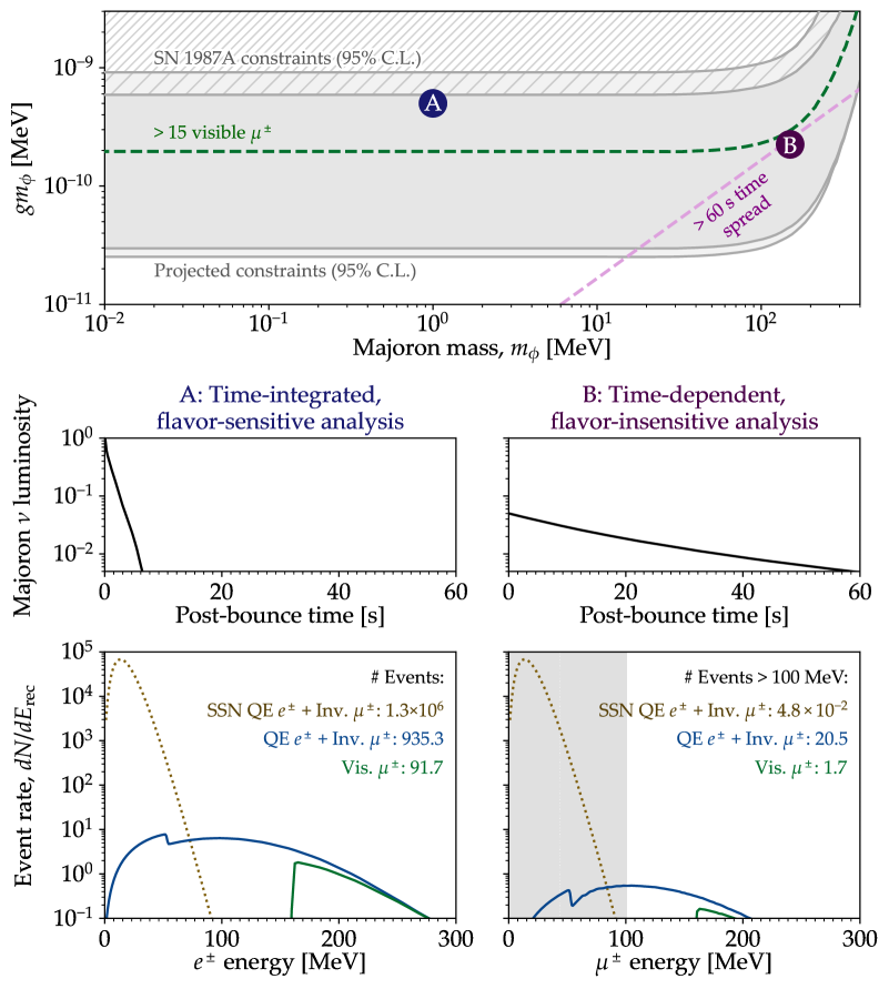
Figure 2: A schematic of our analysis in the Majoron–neutrino coupling parameter space. Top panel: The plane $gm_{\phi}$–$m_{\phi}$ of flavor-universal coupling, $g$, and Majoron mass, $m_{\phi}$, showing current SN 1987A and projected flavor-universal constraints. Flavor-dependent coupling analysis is possible with a high-enough Visible $\mu^{\pm}$ event rate, illustrated with the contour showing $>15$ visible muons. A mass-reconstruction analysis using timing information is possible with a long-enough time spread, illustrated with the contour showing a $>60$ s time spread. The lower panels show the timing (middle) and energy (bottom) distributions of neutrinos predicted for the time-independent, flavor-sensitive benchmark (left), and the time-dependent, flavor-insensitive benchmark (right). For the energy spectrum, we also show results for the Standard SN (SSN) neutrinos, exclusively for the QE $e^{\pm}$ + Inv. $\mu^{\pm}$ signal.

Figure 2 sketches our analysis, which is two-fold, depending on the size of the couplings:

Time-integrated, flavor-sensitive analysis

For large enough couplings, large samples of detected events will be available that could allow us not only to detect the high-energy, non-standard signal from Majoron decays, but also to reconstruct, at least in part, the flavor structure of the coupling, i.e., to measure the values of the couplings of the different neutrino flavors, $g_{e}$, $g_{\mu}$, and $g_{\tau}$, individually. Because, for such large couplings, the typical time spread of the neutrinos from Majoron decay is short compared to the duration of the standard SN neutrino signal, we perform a time-integrated analysis. Our sensitivity is driven by the interplay of the QE $e^{\pm}$ + Inv. $\mu^{\pm}$ and visible $\mu^{\pm}$ channels, which are sensitive to different flavors (Section 4). In Fig. 2, we identify coarsely the region in the parameter space of Majoron mass and coupling (flavor-universal coupling, for illustration) where such a time-integrated, flavor-sensitive analysis is viable due to there being more than $15$ high-energy detected visible muons from Majoron decay.

Time-dependent, flavor-insensitive analysis

For a sufficiently small value of the coupling $g$, the Majoron time spread estimated in Section 2 can become larger than the standard duration of the burst. While the number of detected events is lower in this region of the parameter space, the time structure of the detected neutrino signal would provide a direct probe of the size of the coupling, whereas the number of detected events would depend primarily on the combination $gm_{\phi}$ of coupling and mass. We will show that this allows for a clear disentangling of the two parameters and, therefore, an explicit reconstruction of the Majoron mass. In Fig. 2, this region of the parameter space is coarsely identified by the requirement that the typical time spread, $m_{\phi}/2\Gamma_{\phi}E_{\nu}$, is larger than $60$ s for a 100-MeV neutrino.

When real data become available, a complete time-dependent analysis with flavor sensitivity might provide more detailed information. Today, however, this poses serious technical challenges, since there is no flexible parametrization for the time- and energy-dependent signal from a SN. Nevertheless, our approach needs not face these challenges, instead using the conservative strategy based on the separation between the energies of the standard and non-standard neutrinos.

5.1 Time-integrated, flavor-sensitive analysis

5.1.1   Bounds from the non-observation of high-energy neutrinos

Before asking the question of how well one could reconstruct the Majoron properties in case a high-energy SN neutrino signal were observed, we deal with the more pessimistic scenario in which no such signal is observed. In this case, the next galactic SN will still provide novel bounds on the Majoron coupling more powerful than the current ones.

Previously, Refs. [74, 154] reported projected bounds from a galactic SN. Here, we independently compute projected bounds. We make projections assuming both the cold and hot models, while Ref. [74] used the cold model only and Ref. [154] used a model of electron-capture SN with a very low progenitor mass [168], using an equation of state nowadays not strongly favored [169]; apart from this, such a model should give results quite close to the cold model given the similar PNS mass. Further, Refs. [74, 154] considered only the QE $e^{\pm}$ + Inv. $\mu^{\pm}$ topology, although this should not affect too much the bounds which are sensitive to the total number of non-standard events, largely dominated by this class of events.

Bounds from SN 1987A

First, we obtain present-day bounds on the Majoron mass and coupling using the SN 1987A observations. These bounds were obtained in Ref. [43] for the case of $g_{e}=g_{\mu}=g_{\tau}$. We follow closely the same procedure, but extend it to the case where $g_{e}$, $g_{\mu}$, and $g_{\tau}$ can be different from one another. For the bounds based on the legacy data from SN 1987A we use only the $e^{\pm}$ signal from QE scattering detected by Kamiokande and IMB, and neglect the visible muons due to the uncertainties in how the detectors would have seen such a signal.

We briefly summarize the statistical procedure here, emphasizing the few differences with Ref. [43]. We use the unbinned likelihood function

$$\mathcal{L}\left(g_{\alpha},m_{\phi};\bm{\theta}_{\mathrm{SN}},\bm{\theta}_{\mathrm{mix}}\right)=\; \mathrm{exp}\left(-\int_{E_{\rm min}}^{E_{\rm max}}dE_{\rm rec}\frac{dN_{\rm QE}}{dE_{\rm rec}}\right)\prod_{k}\frac{dN_{\rm QE}}{dE_{\rm rec}}(E_{k})$$

$$\times\pi_{12}(\theta_{12})\pi_{13}(\theta_{13})\pi_{23,{\rm CP}}(\theta_{23},\delta_{\rm CP})\;,$$ (5.1)

where $E_{\rm rec}$ is the reconstructed energy of the event, ${dN_{\rm QE}}/{dE_{\rm rec}}$ is the event rate in the QE $e^{\pm}$ + Inv. $\mu^{\pm}$ detection channel, Eqs. (4.1), (4.5), and (4.10), and $E_{k}$ is the observed energy of each event at Kamiokande and IMB. The minimum energy $E_{\rm min}$ is chosen for each experiment following the prescription in Ref. [43], chosen to minimize the contamination from background. The maximum energy $E_{\rm max}=600$ MeV, but the results are independent of this value since the signal peaks at approximately $150$ MeV. In the likelihood, we make explicit the dependence on the Majoron couplings and mass, $g_{\alpha}$ and $m_{\phi}$, the parameters of the standard SN flux [Eq. (3.1)], $\bm{\theta}_{\mathrm{SN}}=\left\{E_{\mathrm{tot}},E_{0},\alpha\right\}$, and the neutrino mixing parameters that parametrize the PMNS matrix [170], $\bm{\theta}_{\mathrm{mix}}=\left\{\theta_{12},\theta_{13},\theta_{23},\delta_{\rm CP}\right\}$. Differently from Ref. [43], we also introduce pull factors, $\pi$, that evaluate the probability distribution function (PDF) of the mixing parameters. For these, we adopt the $\chi^{2}$ distributions from the NuFit 5.2 global fit to oscillation data, assuming normal neutrino mass ordering [171, 172]. For the mixing parameters $\theta_{12}$ and $\theta_{13}$, the PDFs are one-dimensional; for $\theta_{23}$ and $\delta_{\rm CP}$, the joint PDF is two-dimensional, since they are highly correlated. In the case of flavor-universal couplings studied in Ref. [43], the neutrino flux at Earth is independent of the mixing matrix, so the pull factors were inessential and not used. In our analysis, this is no longer true.

To obtain the bounds, for each trial value of $g_{\alpha}$ and $m_{\phi}$ we compute the profiled likelihood $\overline{\mathcal{L}}(g_{\alpha},m_{\phi})=\mathrm{max}_{\theta_{\mathrm{SN}},\theta_{\mathrm{mix}}}\mathcal{L}$. The one exception is that we do not profile over the value of the pinch parameter, $\alpha$, since the sparse data of SN 1987A are essentially insensitive to it [173, 83]. Instead, we use the fixed value of $\alpha$ for the hot and cold SN models reported in Section 3. For each value of $m_{\phi}$, the likelihood is maximum for vanishing values of $g_{\alpha}$, confirming that the SN 1987A detection did not provide any hint of Majorons. Therefore, we define the test statistic (TS), $\mathrm{TS}(g_{\alpha},m_{\phi})=-2\,\left(\log\left[\overline{\mathcal{L}}(g_{\alpha},m_{\phi})\right]-\log\left[\mathrm{max}_{g_{\alpha}}(\overline{\mathcal{L}}(g_{\alpha},m_{\phi}))\right]\right)$. Under the null hypothesis that a Majoron with parameters $g_{\alpha}$ and $m_{\phi}$ exists, for each value of $m_{\phi}$ the value of TS should be distributed as a half-$\chi^{2}$ distribution (i.e., $\chi^{2}/2$) with one degree of freedom [174]. To obtain the bounds, we set the $95\%$ confidence level (C.L.) threshold value, $\mathrm{TS}(g_{\alpha},m_{\phi})=2.7$.

Figure 3 shows the bounds we obtain for four benchmark cases of the flavor texture of the couplings: universal flavor couplings ($g_{e}=g_{\mu}=g_{\tau}$, as in Ref. [43]), $\nu_{e}$-only coupling ($g_{e}\neq 0$, $g_{\mu}=g_{\tau}=0$), $\nu_{\mu}$-only coupling ($g_{\mu}\neq 0$, $g_{e}=g_{\tau}=0$), and $\nu_{\tau}$-only coupling ($g_{\tau}\neq 0$, $g_{e}=g_{\mu}=0$). We show bounds separately under the assumptions that the neutrinos from Majoron decay are produced in the cold and hot SN models. The bounds made in the cold and hot model, respectively, should then be interpreted as being conservative and aggressive.

For the flavor-universal case, we reproduce the results of Ref. [43], as expected, since we follow the same procedure, up to the anticipated $10\%$ differences induced by the different treatment of Majoron production from $\nu_{\tau}$. For the cold model, the Majorons produced from $\nu_{e}\nu_{e}$ coalescence are by far the dominant ones. Hence, the case $g_{e}\neq 0$ alone leads to bounds that are even more restrictive than the flavor-universal case, because the rate of Majoron production is mostly unchanged but the flavor composition in the decay contains more $\overline{\nu}_{e}$ at Earth, which contribute to the largest detection channel, IBD. For the same reason, the cases $g_{\mu}\neq 0$ and $g_{\tau}\neq 0$ lead to significantly weaker bounds, since they are worsened both by the much lower Majoron production and fraction of $\overline{\nu}_{e}$ at Earth. For the hot model, the Majoron production from $\nu_{\mu}\nu_{\mu}$ coalescence is nearly comparable with the production from $\nu_{e}\nu_{e}$ coalescence, due to the high temperatures in the SN core that lead to the build-up of a degenerate $\overline{\nu}_{\mu}$ population. Therefore, the bounds for $g_{\mu}\neq 0$ and $g_{\tau}\neq 0$ are quite closer to the bounds for $g_{e}\neq 0$.

Reference [74] obtained bounds on the Majoron couplings akin to ours, for the cold model only, and with some differences. The bounds are comparable (see Fig. 5 in Ref. [74]), but ours are weaker by about $40\%$, implying a difference of nearly a factor of $2$ in the event rate. Since for SN 1987A we use the same strategy as Ref. [43], which Ref. [74] also follows, this difference is probably not due to the analysis procedure. When computing Majoron production, Ref. [74] used the neutrino chemical potentials from a digitized version of the contour plots in Ref. [43] which likely introduced imprecision in their values that led to the discrepancy in the bounds [175].

Projected bounds

Having obtained the present-day bounds, we can now obtain projected ones. We consider all the event topologies introduced earlier (Section 4.1) to compute the event rates following the procedure in Section 4.3. We build a mock event sample by simulating the response of the detector to a hypothetical next galactic SN located at a distance $d=10$ kpc. We assume the next galactic SN to match the cold or the hot model in turn. In simulating the signal we are not being conservative or aggressive, since this choice does not determine the strategy of analysis; in the analysis, we are always conservative and assume no knowledge of the simulated SN model. Our choice only determines whether the next galactic SN will be a cold or a hot one, bracketing the range of possibilities.

For each of the simulated SN models, we consider only the Asimov data sample, namely, that the experiment will detect a signal exactly equal to the expected one [174]. In principle, the real signal might fluctuate around its mean, but the projected bounds are dominated by the high-energy region, above $100$ MeV, where the standard flux produces essentially no expected events and therefore fluctuations are irrelevant. Even for our discovery prospects (Sections 5.1.2 and 5.2), we neglect fluctuations away from the Asimov data sample, with the understanding that they may shift the best-fit values of the Majoron mass and coupling.

The expected value of the log-likelihood function, which is the quantity used to set the bounds (see, e.g., the discussion in Section IV.B of Ref. [176]), is

$$\begin{split}\chi^{2}(g_{\alpha},m_{\phi})=&-2\,\mathrm{max}_{\bm{\theta}_{\mathrm{SN}}}\langle\log\mathcal{L}\left(g_{\alpha},m_{\phi};\bm{\theta}_{\rm SN}\right)\rangle\\ =&-2\sum_{\rm t}\left[\int_{0}^{E_{\rm max}}dE_{\rm rec}\,\frac{dN_{\rm t,true}}{dE_{\rm rec}}\,\text{ln}\left(\frac{dN_{\rm t,test}(g_{\alpha},m_{\phi};\bm{\theta}_{\mathrm{SN}})}{dE_{\rm rec}}\right)\right.\\ &\left.-\int_{0}^{E_{\rm max}}\,dE_{\rm rec}\,\frac{dN_{\rm t,test}(g_{\alpha},m_{\phi};\bm{\theta}_{\mathrm{SN}})}{dE_{\rm rec}}\right]\;,\end{split}$$ (5.2)

where $\langle\log\mathcal{L}\rangle$ is the likelihood function averaged over all possible realizations of the true distribution of the events—which corresponds to using the Asimov data sample—and $dN_{\rm t,test}/dE_{\rm rec}$ is the rate of events of topology t, evaluated at test values $g_{\alpha}$ and $m_{\phi}$ and test values of the SN parameters $\bm{\theta}_{\rm SN}$. The latter includes, as before, the parameters of the standard SN flux, $E_{\rm tot}$, $E_{0}$, and $\alpha$ (though $\alpha$ remains fixed, as for the SN 1987A bounds), but now also includes the choice between the hot and cold SN model, which we profile over when computing bounds. Similarly, $dN_{\rm t,true}/dE_{\rm rec}$ is the event rate evaluated at the assumed “true” values of the parameters. In Eq. (5.2), we set the maximum energy of integration to $E_{\rm max}=600$ MeV for the QE $e^{\pm}$ + Inv. $\mu^{\pm}$, visible $\mu^{\pm}$, and electron scattering channels, and to 10 eV for CE$\nu$NS; these choices cover the full width of the event energy distributions. Like before, we define a test statistic,

$$\mathrm{TS}(g_{\alpha},m_{\phi})=\chi^{2}(g_{\alpha},m_{\phi})-\chi^{2}(\hat{g}_{\alpha},m_{\phi})\;,$$ (5.3)

where $\hat{g}_{\alpha}$ is the best-fit value of the coupling. We compute constraints for varying values of $m_{\phi}$. Because we use Asimov data samples, the best-fit value of the coupling always coincides with the assumed true value. We fix the mixing parameters to their present-day best-fit values from NuFit 5.2 [171, 172], assuming normal mass ordering, but ignore the future uncertainty on them, since we expect that it will be sizably reduced by upcoming oscillation experiments [177]. Like for the SN 1987A bounds, we set the $95\%$ C.L. threshold at ${\rm TS}(g_{\alpha},m_{\phi})=2.7$.

To compute the projected bounds, we assume as true values $g_{\alpha}=0$. The set of simulated SN parameters, $\bm{\theta}_{\rm SN}$, corresponds to the choice between the cold or hot SN model. However, regardless of the choice of the true SN model, we always profile the likelihood over both the hot and cold models. In fact, profiling over the SN model in our analysis is perhaps an overly conservative step, since in reality the large standard SN signal would presumably allow us to infer quite precisely the mass of the PNS and to understand whether the SN was truly closer to a cold or a hot model. Thus, our projected bounds are conservative, since they do not assume knowledge of the SN model.

Figure 3 shows that the resulting projected bounds are a substantial improvement over the SN 1987A bounds. The improvement can be understood from simple order-of-magnitude estimates. Since the volume we use for Hyper-Kamiokande is $55$ times larger than the $6.8$ kton volume of IMB, we expect an improvement in the bounds of a factor of $\sqrt{55}\approx 7$. Our simulated SN is placed at a distance of $10$ kpc, shorter by a factor $5$ than SN 1987A, leading to an additional improvement of a factor of $5$. This totals an improvement of a factor $35$ in the bounds, in agreement with the results of our full numerical analysis in Fig. 3. Our bounds differ from those of Ref. [154], as pointed out in Section 4.2.3.

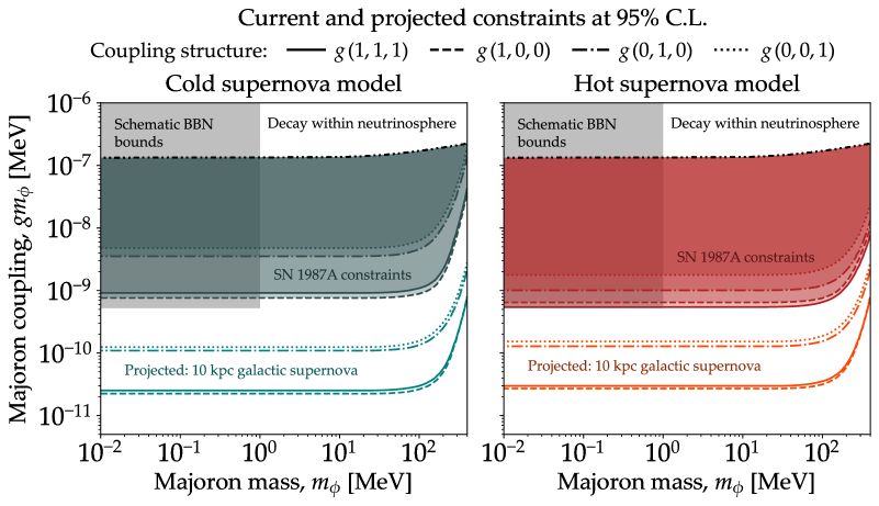
Figure 3: Majoron mass and coupling constraints from SN 1987A data and from a projected next galactic SN at 10 kpc. The schematic BBN bounds are taken from [43]. Above $gm_{\phi}\sim 10^{-7}$ MeV, our bounds do not apply due to trapping since Majorons decay within the neutrinosphere. The SN 1987A bounds are obtained assuming that the SN was cold (left) or hot (right); hence, they are conservative and aggressive. The projected bounds are obtained assuming that the next galactic SN will be cold (left) or hot (right), but in both cases we do not assume knowledge of the model in the analysis; hence, the bounds are pessimistic and optimistic but in both cases conservative.

5.1.2   Measuring couplings to different neutrino flavors

If a sufficiently large high-energy neutrino flux is detected, the different detection channels allow for a partial reconstruction of the flavor structure of the Majoron couplings. To quantify this, we simulate the neutrino signal detected from the decay of a Majoron with $m_{\phi}=1$ MeV and $gm_{\phi}=5\times 10^{-10}$ MeV, which is currently not excluded, but lies near the edge of the most aggressive present-day bounds (Fig. 3). For Majoron masses $m_{\phi}<10$ MeV, the event rate is essentially independent of the mass, so the results would be identical for any other value of the Majoron mass in this range. We adopt only the cold SN model as true, though we still profile the likelihood over the hot and cold models. This makes our projections pessimistic, since if a hotter SN exploded instead, we would expect higher event rates and more precise measurements.

In reconstructing the flavor structure of the couplings, we are faced with a Majoron parameter space including three diagonal couplings, $g_{e}$, $g_{\mu}$, and $g_{\tau}$, and the Majoron mass, $m_{\phi}$. In principle, there could be additional off-diagonal couplings of the form $g_{\alpha\beta}$, with $\alpha\neq\beta$, that violate lepton-flavor conservation; however, we choose to fix them to zero in our work [Eq. (1.1)]. A comprehensive analysis of the entire parameter space would presumably be instructive to perform with real data. When making projections, such an analysis would only widen the parameter space and make the results less intuitive. Hence, we focus on a corner of the parameter space where $g_{e}$, $g_{\mu}$, or both are the only nonzero couplings, and we treat them as free parameters whose values we will determine.

For the light Majorons that we consider for this analysis, with $m_{\phi}<10$ MeV, the energy spectrum and time distribution of the neutrinos from their decay are essentially independent of the value of $m_{\phi}$ as discussed in Ref. [43], so we do not expect to have a strong sensitivity to its value. In addition, discriminating between $g_{\mu}$ and $g_{\tau}$ is challenging, since, because the mixing between them is near-maximal due to $\theta_{23}\approx 45^{\circ}$, they lead to similar flavor composition at Earth and, for the cold model, even similar Majoron production rates, as discussed in Section 2. We simulate three benchmark cases, corresponding to the coupling structures $(g_{e},g_{\mu},g_{\tau})=g\,(1,1,0)$, $g\,(1,0,0)$, and $g\,(0,1,0)$, where $g$ is the parameter whose value we float.

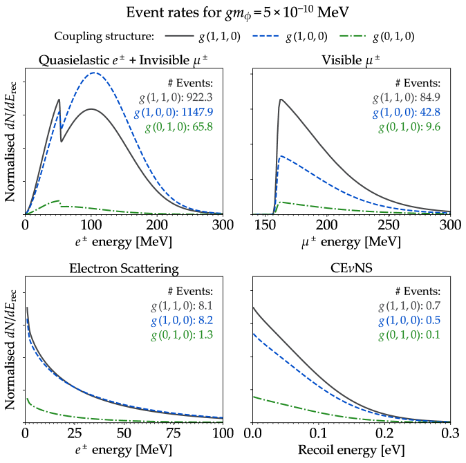
Figure 4: Flavor-dependent analysis benchmark event rates in each of the detection topologies. We simulate a light Majoron with a mass of $m_{\phi}=1$ MeV, with couplings allowed by current SN 1987A bounds of $gm_{\phi}=5\times 10^{-10}$ MeV. For the pessimistic choice $gm_{\phi}=2\times 10^{-10}$ MeV (not shown), the flux trivially scales with the square of the coupling. Events were simulated assuming a cold SN model.

Figure 4 shows the event rates for all three cases. First, there is a clear dependence of the total number of events on the coupling structure, which is understood based on our earlier analysis of the Majoron signal: for the cold model, a nonzero coupling to $\nu_{e}$ only leads to a much larger event rate than a nonzero coupling to $\nu_{\mu}$. When only $g_{e}\neq 0$, the event rates are larger than when both $g_{e}$ and $g_{\mu}$ are nonzero and equal, since in the latter case, for the cold model, the additional small Majoron emission from $\nu_{\mu}\nu_{\mu}$ coalescence in the SN is offset by the enhanced fraction of $\overline{\nu}_{e}$ for Majoron decay to $\overline{\nu}_{e}+\overline{\nu}_{e}$.

However, the absolute number of events cannot discriminate different coupling structures, since it is degenerate with the unknown absolute value of the coupling. Luckily, we easily identify other features of the signal that break the degeneracy: the height of the peak of Michel electrons and positrons relative to the peak of the event rate in the QE $e^{\pm}$ + Inv. $\mu^{\pm}$ channel, and number of events in the visible $\mu^{\pm}$ channel are good proxies of the fraction of muon neutrinos at Earth. The number of events in the ES channel could also be a good proxy of the all-flavor flux, but the event rates are low even for our optimistic benchmark case with the largest coupling. Finally, for CE$\nu$NS, less than one event is expected in all cases, so this channel does not play a role in our analysis.

For the statistical analysis, we use the same definition of the likelihood function as before, in Eq. (5.2), except that it now depends on $g_{e}$ and $g_{\mu}$ separately, and the true flux now includes the standard SN neutrinos from the cold SN model plus the neutrinos from the decay of a light Majoron with $m_{\phi}=1$ MeV (like before, we do not profile the likelihood over $m_{\phi}$). We consider two cases: an optimistic one with $gm_{\phi}=5\times 10^{-10}$ MeV and a pessimistic one with $gm_{\phi}=2\times 10^{-10}$ MeV. For a fixed value of $gm_{\phi}$, the outcome is essentially independent of $m_{\phi}$ unless it is of tens of MeV, where Majoron production starts to be kinematically suppressed. Hence, our projected reconstruction is valid for any Majoron mass lower than tens of MeV and larger than tens of keV, below which it becomes comparable to the neutrino thermal mass; see Section 2. The test statistic, TS, is given by Eq. (5.3), evaluated now at test values of $g_{e}$ and $g_{\mu}$ separately. Since we are no longer setting upper bounds on the couplings (Section 5.1.1), but measuring their values, the TS is expected to follow a $\chi^{2}$ distribution with two degrees of freedom, $g_{e}m_{\phi}$ and $g_{\mu}m_{\phi}$, and so the threshold value for $95\%$ C.L. is TS = 6.

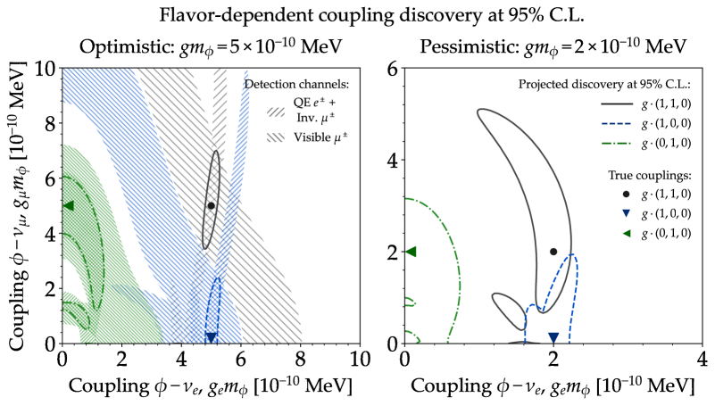
Figure 5: Discovery of a Majoron-neutrino flavor-dependent coupling. We show the $95\%$ C.L. discovery regions for different flavor textures of the Majoron-neutrino coupling, assuming optimistic (left) and pessimistic (right) illustrative values of the coupling.

Figure 5 shows the resulting projected joint allowed regions of $g_{e}m_{\phi}$ and $g_{\mu}m_{\phi}$, for the above optimistic and pessimistic benchmarks of their true values, and assuming three sample flavor textures: pure $g_{e}$ coupling, pure $g_{\mu}$ coupling, and $g_{e}=g_{\mu}$ couplings. For the optimistic benchmark, we also show separately the discovery contours using only events in the QE $e^{\pm}$ + Inv. $\mu^{\pm}$ channel and in the visible $\mu^{\pm}$ channel, to highlight their contributions. For this benchmark, the large number of detected events allows for a precise measurement of the couplings, thanks to the complementary information carried by the different topologies. The QE $e^{\pm}$ + Inv. $\mu^{\pm}$ channel yields a narrow interval of $g_{e}$, since even a tiny increase or decrease in $g_{e}$ would dramatically alter the expected number of high-energy neutrino events in this topology. However, this channel alone provides nearly no sensitivity to $g_{\mu}$, which is provided by visible $\mu^{\pm}$. Moreover, Fig. 5 shows that the three sample flavor textures can be discriminated from one another.

For the pessimistic benchmark, the event rates are reduced by more than a factor $4$ due to the lower coupling, and the allowed regions of $g_{e}m_{\phi}$ and $g_{\mu}m_{\phi}$ are widened. The allowed regions are characteristically multi-humped, and in the $g(1,1,0)$ they become even disconnected, due to profiling the likelihood function over the cold and hot SN models. As we stated out earlier, even though we adopt the cold SN model as the true one when generating our mock observations, we assume no knowledge of the SN model in the statistical analysis. This allows us to explain the mock observations also using the hot SN model with lower values of the couplings compared to those preferred by the cold SN model. As pointed out in Section 5.1.1, this is an overly conservative step, since in reality the information from the low-energy standard SN events would allow us to resolve the mass of the PNS, and to discriminate between the hot and cold models. Regardless, even in the pessimistic benchmark, the three sample flavor textures may be discriminated from each other.

5.2 Time-dependent, flavor-insensitive analysis

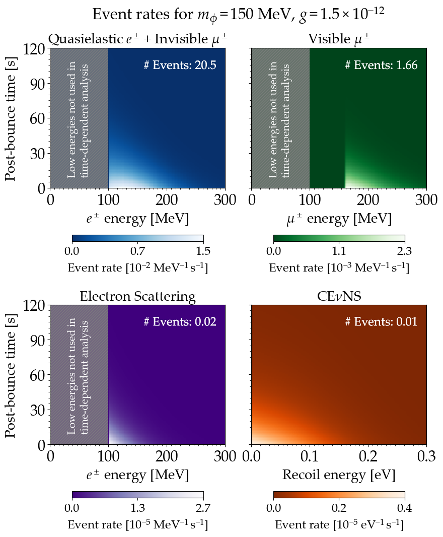
Figure 6: Timing-dependent analysis benchmark event rates for each detection topology. We simulate a Majoron of $m_{\phi}=150$ MeV with flavor-universal coupling $g=1.5\times 10^{-12}$. The gray bars indicate the energy cut of our analysis that removes events below $100$ MeV in order to eliminate the standard SN neutrino flux. We show the electron scattering and CE$\nu$NS event rates here, but do not include them in our analysis.

Majorons are produced mostly in the very first second post-bounce in the SN core, when neutrinos are strongly degenerate. Therefore, if a high-energy neutrino flux from their decay were to be observed over a much longer duration, at several tens of seconds post-bounce, this would be a natural indication that the Majoron is heavy. Measuring the time scale would allow us to break the degeneracy between the Majoron coupling and mass that would otherwise exist. Crucially, however, detecting neutrinos at these late times is not by itself a unique signature of the presence of Majorons, since standard late-time SN emission from fallback accretion is possible (Section 4.2.3). Only by virtue of their high energies we can be sure of their origin.

Disentangling the neutrinos from Majoron decay from the standard SN neutrinos is a more complex task in a time-dependent analysis than in our earlier time-integrated one. While the standard neutrino fluence in the cooling phase is described well by Eq. (3.1), there is no available parametrization of the time-dependent flux. This situation is even worse for the late-time neutrino emission. We circumvent this limitation by cutting from our analysis all events with energies below $100$ MeV, so that the expected number of events from Majoron decay across all topologies is $52.4$ for the hot model and 22.2 for the cold model, while the expected number of standard SN events is, respectively, only $6.5$ and 0.05, less than the Poisson fluctuations on our signal. The potential contamination from late-time fallback accretion has typically even lower energy than during the cooling phase. Thus, in our analysis we neglect the standard SN contamination above 100 MeV. This hard cut in energy is conservative, meant to show the potential of a time-dependent analysis. In reality, below $100$ MeV the neutrinos from Majoron decay exhibit unique signatures, such as the characteristic shape of the spectrum of Michel positrons from the decay of higher-energy muons, that could be used to identify them even in the absence of a parametrization of the time-dependent standard SN flux.

Figure 6 shows the distributions in time and energy of the expected events, for the cold SN model, and for benchmark choices of the model parameters. We adopt a benchmark heavy Majoron with flavor-universal couplings of $g_{e}=g_{\mu}=g_{\tau}\equiv g=1.5\times 10^{-12}$ and mass of $m_{\phi}=150$ MeV. The only two topologies with a detectable number of events are QE $e^{\pm}$ + Inv. $\mu^{\pm}$ and visible $\mu^{\pm}$. As the coupling considered is small, electron scattering and CE$\nu$NS yield negligible event rates.

Since we discard the standard neutrinos above 100 MeV, only the neutrinos from Majoron decay contribute to the event rates. We define the likelihood function in analogy to Eq. (5.2), but now using the joint energy and time distribution of the events, i.e.,

$$\begin{split}\chi^{2}(g,m_{\phi})=&-2\,\mathrm{max}_{\bm{\theta}_{\mathrm{SN}}}\langle\log\mathcal{L}\left(g,m_{\phi};\bm{\theta}_{\rm SN}\right)\rangle\\ =&-2\sum_{\rm t}\left[\int dt\int_{90\;\mathrm{MeV}}^{E_{\mathrm{max}}}dE_{\rm rec}\,\frac{dN_{\rm t,true}}{dtdE_{\rm rec}}\,\text{ln}\left(\frac{dN_{\rm t,test}(g,m_{\phi};\bm{\theta}_{\mathrm{SN}})}{dtdE_{\rm rec}}\right)\right.\\ &\left.-\int\,dt\int_{90\;\mathrm{MeV}}^{E_{\mathrm{max}}}dE_{\rm rec}\,\frac{dN_{\rm t,test}(g,m_{\phi};\bm{\theta}_{\mathrm{SN}})}{dtdE_{\rm rec}}\right]\;,\end{split}$$ (5.4)

where now $\bm{\theta}_{\rm SN}$ represents the choice between the cold and hot SN models. In analogy to Eq. (5.3), the test statistic is

$$\mathrm{TS}(g,m_{\phi})=\chi^{2}(g,m_{\phi})-\chi^{2}(\hat{g},\hat{m}_{\phi})\;,$$ (5.5)

where, unlike our earlier analyses, we now minimize TS simultaneously over $g$ and $m_{\phi}$; in Eq. (5.5), $\hat{g}$ and $\hat{m}_{\phi}$ are their best-fit values, which coincide with the true values. We evaluate the true event spectrum at the same benchmark choices of the model parameters as in Fig. 6 and the test event rate at test values of $g$ and $m_{\phi}$. The TS is obtained by profiling over the SN hot and cold models; it is expected to follow a $\chi^{2}$ distribution with two degrees of freedom, so the regions of $g$ and $m_{\phi}$ allowed at $95\%$ C.L. are obtained by setting $\mathrm{TS}=6$.

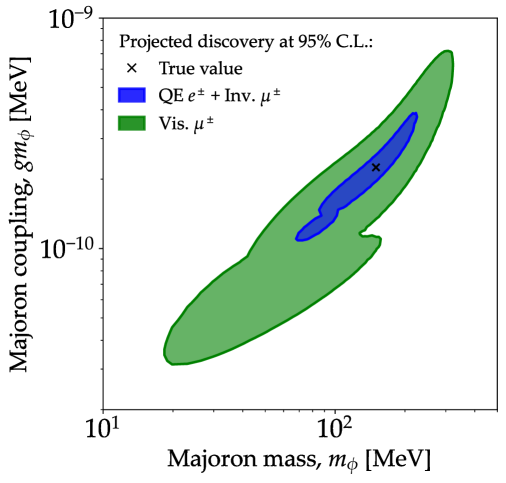
Figure 7: Majoron mass reconstruction. The measurement is based on our time-dependent, flavor-insensitive analysis strategy. The true, simulated Majoron mass and flavor-universal coupling are $m_{\phi}=150$ MeV and $g=1.5\times 10^{-12}$. We show separately the result of using the two topologies with the highest event rates: QE $e^{\pm}$+Inv. $\mu^{\pm}$ and visible $\mu^{\pm}$.

Figure 7 shows the $95\%$ C.L. allowed regions of the Majoron mass and coupling. We show separate contours for the two visible detection channels, but the sensitivity of reconstruction is driven primarily by the QE $e^{\pm}$ + Inv. $\mu^{\pm}$ channel due to its much higher rate. The Majoron mass is reconstructed to within about 60% of its true value. The allowed region is two-humped, with the two humps resulting from profiling over the hot and cold SN models. This is because, even if the simulated SN assumed the cold model, the observed SN signal can also be explained with a lower coupling if the original SN model was hot. As stated previously, in reality, thanks to the copious low-energy SN neutrinos, we should be able to assert whether the model was truly cold or hot, and thus the allowed region would be smaller.

6 Summary and outlook

It is general agreement that a copious detection of neutrinos from the next galactic supernova (SN) will be a powerful testbed for new physics. However, this statement is sometimes used as an overly optimistic motto, especially since many of the observables currently used to probe new physics would not benefit significantly from a signal seen with a large number of detected events. A paradigmatic example is the celebrated SN 1987A cooling bound [18], based on the duration of the neutrino burst. This constraint is presumably not limited by experimental uncertainties—after all, the detected neutrino events were sufficient to pinpoint the duration of the SN 1987A burst certainly to within a factor of 2—but rather by theoretical ones, since convection and neutrino-nucleon opacities seem to play the key role in shaping the duration of the cooling phase [83], an aspect unaccounted for in the historical studies of the cooling bounds. The main possibility to learn about beyond the Standard Model (BSM) physics from the boon of neutrino data expected from the next galactic SN is to directly detect the neutrinos produced in the decay of Majorons or other feebly interacting particles. This strategy would benefit from a large event rates, leading either to much more stringent bounds or to a discovery. Making best use of this possibility requires a concrete strategy relating the properties of the BSM model to the observables of the neutrino signal, marginalizing over our ignorance of the SN physics details. This is the open question we tackled in this work.

We have considered the production of high-energy Majorons via the coalescence of neutrinos inside the proto-neutron star (PNS) of a SN. For this setup, the lepton number violation maximizes the energy of the BSM neutrinos, which are produced primarily from the coalescence of $\nu_{e}$ with large chemical potential. The subsequent decay of the Majorons into neutrinos leads to a high-energy component in the flux observable at Earth. Each neutrino event detected in ongoing and planned neutrino and dark matter experiments will be characterized by a limited number of features, namely its energy, the event topology in the detector, and the time of arrival. Compared to the existing literature, we exploit for the first time all these features to reconstruct the properties of the underlying BSM model, i.e., the mass of the Majoron and its couplings to $\nu_{e}$, $\nu_{\mu}$, and $\nu_{\tau}$.

We have geared our forecasts to the detection of SN neutrinos by upcoming observatories Hyper-Kamiokande and DARWIN. They provide sensitivity to multiple neutrino detection channels: Hyper-Kamiokande, to quasi-elastic (QE) $\nu_{e}$ and $\nu_{\mu}$ scattering, and to neutrino–electron ES, and DARWIN, to coherent elastic neutrino-nucleon scattering (CE$\nu$NS). Combined, the different detection channels grant us partial sensitivity to the flavor composition of the SN neutrino flux. Concretely, we gain access to the content of $\nu_{e}$ and $\nu_{\mu}$ in the flux by contrasting the number of detected high-energy visible muons, the number of events from $\nu_{e}$ QE scattering, and the height of the peak of Michel $e^{\pm}$ coming from invisible muon decays relative to the remaining $\nu_{e}$ QE scattering events. At high energies, the expected rate of CE$\nu$NS events is, unfortunately, negligible.

The only observable that allows us to unambiguously distinguish the standard SN neutrino flux from the neutrinos produced by Majoron decay is the energy spectrum. As pointed out in Refs. [75, 43], neutrinos from Majoron decay have energies higher ($\sim 100\,\rm MeV$) than standard SN neutrinos ($\sim 10\,\rm MeV$). The possibility of measuring the energy of individual neutrinos allows us to obtain results that depend only weakly on the uncertainties in the standard SN neutrino production.

We have shown the potential use of the signal from the next galactic SN via three separate kinds of analyses. In the first analysis, we focus on the negative viewpoint that no high-energy neutrino will be observed, in which case we will only obtain bounds on BSM physics. While this is a possibility, the best-case scenario would of course be the one in which a signal is observed. Therefore, our second and third analyses refer to the case in which a high-energy neutrino signal will be detected from the next galactic SN. Below, we detail each of these analyses.

First, in case no event with a particularly high energy is observed, we can constrain Majoron couplings to neutrinos of different flavors. Such bounds rely on two observables—the energy spectrum and the topologies of the detected events. We have revisited the projected bounds on heavy Majorons by considering two largely different cases for the PNS profiles of density and temperature, a cold and a hot simulated model. The bounds we find on the couplings are consistent with simple order-of-magnitude estimates, and highlight the dependence on the flavor texture of the couplings. In our analysis we are overly conservative, assuming that we have no knowledge of the mass of the PNS, which determines the typical temperature and luminosity of the model; practically, we always profile over the hot or cold model. In reality, the large standard neutrino signal in the tens-of-MeV energy range would allow us to pinpoint the mass of the PNS and potentially improve the bounds, especially if the next galactic SN involves a heavy PNS.

Second, for a large coupling, many neutrinos from Majoron decays will be observed in all the different topologies within a span of a few seconds. For this scenario, we show that the combining different event topologies allows us to reconstruct the separate couplings $g_{e}m_{\phi}$ and $g_{\mu}m_{\phi}$. Extending this analysis to more general coupling structures would presumably be more useful to pursue in case of a real observation; here we show as a proof of principle that a partial flavor structure reconstruction of the model is possible with the expected event rates, focusing on couplings of the order of $g_{\alpha}m_{\phi}\sim 10^{-10}$ MeV.

Third, for large masses and low couplings (our benchmark is a mass $m_{\phi}=150\,\rm MeV$ and a flavor-universal coupling $g=1.5\times 10^{-12}$), the time distribution of the detected events can be stretched by up to tens of seconds. Folding both the time and energy distributions in our analysis allows us to jointly measure the Majoron mass and coupling. The current absence of a parametrization of the time dependence of the standard SN neutrino production motivates us to discard events with energies below 100 MeV from our analysis in order to remove the otherwise dominant standard signal. We show that the timing information can be used to infer the BSM parameters, while the high energy of the events involved guarantees minimal-to-no sensitivity to the SN physics uncertainties.

As a general comment, we are of course unaware of what properties the next galactic SN will have. However, most of our results turn out to be qualitatively independent of this ignorance. For all of our reconstruction prospects, we consider that the next galactic SN will resemble our cold model, which is a pessimistic choice, since a hotter SN would produce a larger signal and allow us to reconstruct the Majoron properties more precisely. We assume that the SN will occur 10 kpc away; for the projected bounds that we draw, the bounds on the couplings scale linearly with the distance. Similarly, if a SN should explode before Hyper-Kamiokande starts operations, one can still benefit from the exposure of its predecessor Super-Kamiokande [178], which is currently active. In that case, the bounds on $g_{\alpha}$ would be worsened by the square root of the effective volume ratio for the two experiments. For the projected reconstruction of the BSM parameters, the impact of a different distance must be assessed by a dedicated analysis. Finally, the next galactic SN might fail to produce a neutron star, with the remnant quickly collapsing into a black hole and interrupting neutrino emission during the cooling of the PNS. This would be to our advantage, since the Majorons would still be produced within the first second, before the collapse to a black hole, while the standard neutrino emission would be cut off, reducing the background for BSM searches.

Overall, for the first time, we have shown that the multiple topologies and timing of the events detected from the next galactic SN could allow us to reconstruct the mass and couplings of Majorons that decay into neutrinos. Our findings can be applied to a plethora of different models positing particles that decay into neutrinos, such as novel gauge bosons or sterile neutrinos.

Appendix A Time distribution of decay neutrinos

In this appendix we derive explicitly the time distribution for the neutrinos produced in the decay of a Majoron. The geometry of the process is illustrated in Fig. 1. We assume the Majoron has an energy $E_{\phi}$ and thus moves with a velocity $v_{\phi}=\sqrt{1-m_{\phi}^{2}/E_{\phi}^{2}}$; we do not assume ultra-relativistic Majorons.

The time delay of a neutrino from the decay of a Majoron, compared to the arrival time of a neutrino moving in straight line, is

$$t=\frac{\ell}{v_{\phi}}+s-D_{\mathrm{SN}}\;,$$ (A.1)

where $\ell$ is the distance that the Majoron travels before it decays and $s$ is the distance that its daughter neutrinos travel from there to the Earth. We can safely assume that $\ell\ll D_{\mathrm{SN}}\sim~{}{\rm kpc}$, since $\ell$ is roughly the size of the decay length of the boosted Majoron, i.e., $\ell_{\phi}\sim E_{\phi}/\sum_{\alpha}g_{\alpha}^{2}m_{\phi}^{2}$. Even for $gm_{\phi}\ll 10^{-12}$ MeV, much lower than what we will be able to probe with future experiments, for a Majoron energy of $E_{\phi}\sim 100$ MeV, this yields $\ell_{\phi}\simeq 2\times 10^{15}~{}{\rm cm}\ll D_{\mathrm{SN}}$. Thus, we can approximate $s\simeq D_{\rm SN}-\ell\cos\alpha\gg\ell$, where $\alpha$ is the angle at which the Majoron is emitted from the PNS, measured with respect to the straight-line distance from the PNS to Earth. It also follows from here that the angle with which the neutrinos arrive at Earth, also measured with respect to the straight-line distance from the PNS to Earth is $\beta\ll 1$; concretely,

$$\beta\simeq\frac{\ell\sin\alpha}{s}\simeq\frac{\ell\sin\alpha}{D_{\rm SN}}\;.$$ (A.2)

With this approximation, the angle $\alpha$ of emission of the Majoron and the angle $\theta$ between its direction and the direction of the neutrinos are nearly identical, since $\beta\ll\alpha$, i.e., $\theta\simeq\alpha$.

We now connect the angle of emission with the energy of the emitted neutrinos. From the kinematics of the Majoron decay, we find that

$$\cos\theta=\frac{1}{v_{\phi}}\left(1-\frac{m_{\phi}^{2}}{2E_{\phi}E_{\nu}}\right)\;.$$ (A.3)

Replacing $s$ and $\alpha$ in Eq. (A.1) yields

$$t=\frac{\ell m_{\phi}^{2}}{2E_{\nu}E_{\phi}v_{\phi}}\;.$$ (A.4)

The time delay is proportional to the length, $\ell$, travelled by the Majoron before it decays. As is well known, this length has a probability distribution $\propto e^{-\ell/\ell_{\phi}}$, i.e.,

$$P(\ell)d\ell=\exp\left(-\frac{\Gamma_{\phi}m_{\phi}\ell}{E_{\phi}v_{\phi}}\right)\frac{\Gamma_{\phi}m_{\phi}}{E_{\phi}v_{\phi}}d\ell\;,$$ (A.5)

where we have multiplied the decay rate, $\Gamma_{\phi}=1/\ell_{\phi}$, by the Lorentz boost factor $E_{\phi}/m_{\phi}$. From here, using Eq. (A.4), the distribution of time delays is

$$P(t)dt=\exp\left[-\frac{2\Gamma_{\phi}E_{\nu}t}{m_{\phi}}\right]\frac{2\Gamma_{\phi}E_{\nu}}{m_{\phi}}dt\;.$$ (A.6)

Since this distribution does not depend on the Majoron energy, but only on the neutrino energy, we can simply multiply it by the neutrino energy spectrum to obtain the joint time and energy distribution of the neutrinos that reach Earth, recovering the result in Eq. (2.5) in the main text.

References

- [1] R. N. Mohapatra et al., Theory of neutrinos: A white paper, Rept. Prog. Phys. 70 (2007) 1757 [hep-ph/0510213].
- [2] V. Cirigliano and M. J. Ramsey-Musolf, Low Energy Probes of Physics Beyond the Standard Model, Prog. Part. Nucl. Phys. 71 (2013) 2 [1304.0017].
- [3] J. M. Berryman et al., Neutrino self-interactions: A white paper, Phys. Dark Univ. 42 (2023) 101267 [2203.01955]. (2022 Snowmass Summer Study).
- [4] T. Asaka and M. Shaposhnikov, The MSM, dark matter and baryon asymmetry of the universe, Phys. Lett. B 620 (2005) 17 [hep-ph/0505013].
- [5] D. Gorbunov and M. Shaposhnikov, How to find neutral leptons of the MSM?, JHEP 10 (2007) 015 [0705.1729]. [Erratum: JHEP 11, 101 (2013)].
- [6] M. Gell-Mann, P. Ramond and R. Slansky, Color Embeddings, Charge Assignments, and Proton Stability in Unified Gauge Theories, Rev. Mod. Phys. 50 (1978) 721.
- [7] E. Witten, Neutrino Masses in the Minimal O(10) Theory, Phys. Lett. B 91 (1980) 81.
- [8] R. N. Mohapatra and G. Senjanovic, Neutrino Mass and Spontaneous Parity Nonconservation, Phys. Rev. Lett. 44 (1980) 912.
- [9] Y. Chikashige, G. Gelmini, R. D. Peccei and M. Roncadelli, Horizontal Symmetries, Dynamical Symmetry Breaking and Neutrino Masses, Phys. Lett. B 94 (1980) 499.
- [10] Y. Chikashige, R. N. Mohapatra and R. D. Peccei, Are There Real Goldstone Bosons Associated with Broken Lepton Number?, Phys. Lett. B 98 (1981) 265.
- [11] G. B. Gelmini and M. Roncadelli, Left-Handed Neutrino Mass Scale and Spontaneously Broken Lepton Number, Phys. Lett. B 99 (1981) 411.
- [12] J. Schechter and J. W. F. Valle, Neutrino Decay and Spontaneous Violation of Lepton Number, Phys. Rev. D 25 (1982) 774.
- [13] H. M. Georgi, S. L. Glashow and S. Nussinov, Unconventional Model of Neutrino Masses, Nucl. Phys. B 193 (1981) 297.
- [14] Y. B. Zeldovich, A. A. Klypin, M. Y. Khlopov and V. M. Chechetkin, Astrophysical constraints on the mass of heavy stable neutral leptons, Sov. J. Nucl. Phys. 31 (1980) 664.
- [15] M. Gronau, C. N. Leung and J. L. Rosner, Extending Limits on Neutral Heavy Leptons, Phys. Rev. D 29 (1984) 2539.
- [16] J. E. Kim, Light Pseudoscalars, Particle Physics and Cosmology, Phys. Rept. 150 (1987) 1.
- [17] E. D. Carlson, Limits on a new U(1) coupling, Nucl. Phys. B 286 (1987) 378.
- [18] G. G. Raffelt, Stars as laboratories for fundamental physics: The astrophysics of neutrinos, axions, and other weakly interacting particles. 5, 1996.
- [19] DELPHI Collaboration, P. Abreu et al., Search for neutral heavy leptons produced in Z decays, Z. Phys. C 74 (1997) 57. [Erratum: Z. Phys. C 75, 580 (1997)].
- [20] L. M. Johnson, D. W. McKay and T. Bolton, Extending sensitivity for low mass neutral heavy lepton searches, Phys. Rev. D 56 (1997) 2970 [hep-ph/9703333].
- [21] NuTeV, E815 Collaboration, A. Vaitaitis et al., Search for neutral heavy leptons in a high-energy neutrino beam, Phys. Rev. Lett. 83 (1999) 4943 [hep-ex/9908011].
- [22] A. D. Dolgov, S. H. Hansen, G. Raffelt and D. V. Semikoz, Heavy sterile neutrinos: Bounds from big bang nucleosynthesis and SN1987A, Nucl. Phys. B 590 (2000) 562 [hep-ph/0008138].
- [23] M. Kachelrieß, R. Tomàs and J. W. F. Valle, Supernova bounds on Majoron emitting decays of light neutrinos, Phys. Rev. D 62 (2000) 023004 [hep-ph/0001039].
- [24] L3 Collaboration, P. Achard et al., Search for heavy neutral and charged leptons in annihilation at LEP, Phys. Lett. B 517 (2001) 75 [hep-ex/0107015].
- [25] Y. Farzan, Bounds on the coupling of the Majoron to light neutrinos from supernova cooling, Phys. Rev. D 67 (2003) 073015 [hep-ph/0211375].
- [26] EXO-200 Collaboration, J. B. Albert et al., Search for Majoron-emitting modes of double-beta decay of 136Xe with EXO-200, Phys. Rev. D 90 (2014) 092004 [1409.6829].
- [27] E. Hardy and R. Lasenby, Stellar cooling bounds on new light particles: plasma mixing effects, JHEP 02 (2017) 033 [1611.05852].
- [28] CMS Collaboration, A. M. Sirunyan et al., Search for heavy neutral leptons in events with three charged leptons in proton-proton collisions at 13 TeV, Phys. Rev. Lett. 120 (2018) 221801 [1802.02965].
- [29] K. Bondarenko, A. Boyarsky, D. Gorbunov and O. Ruchayskiy, Phenomenology of GeV-scale Heavy Neutral Leptons, JHEP 11 (2018) 032 [1805.08567].
- [30] F. Kling and S. Trojanowski, Heavy Neutral Leptons at FASER, Phys. Rev. D 97 (2018) 095016 [1801.08947].
- [31] G. Magill, R. Plestid, M. Pospelov and Y.-D. Tsai, Dipole Portal to Heavy Neutral Leptons, Phys. Rev. D 98 (2018) 115015 [1803.03262].
- [32] P. Ballett, T. Boschi and S. Pascoli, Heavy Neutral Leptons from low-scale seesaws at the DUNE Near Detector, JHEP 03 (2020) 111 [1905.00284].
- [33] ATLAS Collaboration, G. Aad et al., Search for heavy neutral leptons in decays of bosons produced in 13 TeV collisions using prompt and displaced signatures with the ATLAS detector, JHEP 10 (2019) 265 [1905.09787].
- [34] A. De Gouvêa, M. Sen, W. Tangarife and Y. Zhang, Dodelson-Widrow Mechanism in the Presence of Self-Interacting Neutrinos, Phys. Rev. Lett. 124 (2020) 081802 [1910.04901].
- [35] L. Mastrototaro, A. Mirizzi, P. D. Serpico and A. Esmaili, Heavy sterile neutrino emission in core-collapse supernovae: Constraints and signatures, JCAP 01 (2020) 010 [1910.10249].
- [36] M. Escudero and S. J. Witte, A CMB search for the neutrino mass mechanism and its relation to the Hubble tension, Eur. Phys. J. C 80 (2020) 294 [1909.04044].
- [37] K. J. Kelly, M. Sen and Y. Zhang, Intimate Relationship between Sterile Neutrino Dark Matter and Neff, Phys. Rev. Lett. 127 (2021) 041101 [2011.02487].
- [38] V. Brdar, A. Greljo, J. Kopp and T. Opferkuch, The Neutrino Magnetic Moment Portal: Cosmology, Astrophysics, and Direct Detection, JCAP 01 (2021) 039 [2007.15563].
- [39] C. A. Argüelles, N. Foppiani and M. Hostert, Heavy neutral leptons below the kaon mass at hodoscopic neutrino detectors, Phys. Rev. D 105 (2022) 095006 [2109.03831].
- [40] S. A. Kharusi et al., Search for Majoron-emitting modes of 136Xe double beta decay with the complete EXO-200 dataset, Phys. Rev. D 104 (2021) 112002 [2109.01327].
- [41] CUPID-0 Collaboration, O. Azzolini et al., Search for Majoron-like particles with CUPID-0, Phys. Rev. D 107 (2023) 032006 [2209.09490].
- [42] A. M. Abdullahi et al., The present and future status of heavy neutral leptons, J. Phys. G 50 (2023) 020501 [2203.08039].
- [43] D. F. G. Fiorillo, G. G. Raffelt and E. Vitagliano, Strong Supernova 1987A Constraints on Bosons Decaying to Neutrinos, Phys. Rev. Lett. 131 (2023) 021001 [2209.11773].
- [44] D. F. G. Fiorillo, G. G. Raffelt and E. Vitagliano, Large Neutrino Secret Interactions Have a Small Impact on Supernovae, Phys. Rev. Lett. 132 (2024) 021002 [2307.15115].
- [45] P. Carenza, G. Lucente, L. Mastrototaro, A. Mirizzi and P. D. Serpico, Comprehensive constraints on heavy sterile neutrinos from core-collapse supernovae, Phys. Rev. D 109 (2024) 063010 [2311.00033].
- [46] V. Brdar, A. de Gouvêa, Y.-Y. Li and P. A. N. Machado, Neutrino magnetic moment portal and supernovae: New constraints and multimessenger opportunities, Phys. Rev. D 107 (2023) 073005 [2302.10965].
- [47] D. F. G. Fiorillo, G. G. Raffelt and E. Vitagliano, Supernova emission of secretly interacting neutrino fluid: Theoretical foundations, Phys. Rev. D 109 (2024) 023017 [2307.15122].
- [48] S. Sandner, M. Escudero and S. J. Witte, Precision CMB constraints on eV-scale bosons coupled to neutrinos, Eur. Phys. J. C 83 (2023) 709 [2305.01692].
- [49] G. Chauhan, S. Horiuchi, P. Huber and I. M. Shoemaker, Low-Energy Supernovae Bounds on Sterile Neutrinos, 2309.05860.
- [50] J. H. Chang, R. Essig and S. D. McDermott, Supernova 1987A Constraints on Sub-GeV Dark Sectors, Millicharged Particles, the QCD Axion, and an Axion-like Particle, JHEP 09 (2018) 051 [1803.00993].
- [51] P. Carenza, T. Fischer, M. Giannotti, G. Guo, G. Martínez-Pinedo and A. Mirizzi, Improved axion emissivity from a supernova via nucleon-nucleon bremsstrahlung, JCAP 10 (2019) 016 [1906.11844]. [Erratum: JCAP 05, E01 (2020)].
- [52] P. Carenza, B. Fore, M. Giannotti, A. Mirizzi and S. Reddy, Enhanced Supernova Axion Emission and its Implications, Phys. Rev. Lett. 126 (2021) 071102 [2010.02943].
- [53] A. Caputo and G. Raffelt, Astrophysical Axion Bounds: The 2024 Edition, PoS COSMICWISPers (2024) 041 [2401.13728].
- [54] R. Bollig, W. DeRocco, P. W. Graham and H.-T. Janka, Muons in Supernovae: Implications for the Axion-Muon Coupling, Phys. Rev. Lett. 125 (2020) 051104 [2005.07141]. [Erratum: Phys. Rev. Lett. 126, 189901 (2021)].
- [55] D. Croon, G. Elor, R. K. Leane and S. D. McDermott, Supernova Muons: New Constraints on ’ Bosons, Axions and ALPs, JHEP 01 (2021) 107 [2006.13942].
- [56] A. Caputo, G. Raffelt and E. Vitagliano, Muonic boson limits: Supernova redux, Phys. Rev. D 105 (2022) 035022 [2109.03244].
- [57] A. Caputo, G. Raffelt and E. Vitagliano, Radiative transfer in stars by feebly interacting bosons, JCAP 08 (2022) 045 [2204.11862].
- [58] A. Caputo, H.-T. Janka, G. Raffelt and E. Vitagliano, Low-Energy Supernovae Severely Constrain Radiative Particle Decays, Phys. Rev. Lett. 128 (2022) 221103 [2201.09890].
- [59] R. Z. Ferreira, M. C. D. Marsh and E. Müller, Strong supernovae bounds on ALPs from quantum loops, JCAP 11 (2022) 057 [2205.07896].
- [60] W. DeRocco, P. W. Graham, D. Kasen, G. Marques-Tavares and S. Rajendran, Observable signatures of dark photons from supernovae, JHEP 02 (2019) 171 [1901.08596].
- [61] C. S. Shin and S. Yun, Dark gauge boson emission from supernova pions, Phys. Rev. D 108 (2023) 055014 [2211.15677].
- [62] S. Davidson, S. Hannestad and G. Raffelt, Updated bounds on millicharged particles, JHEP 05 (2000) 003 [hep-ph/0001179].
- [63] D. F. G. Fiorillo and E. Vitagliano, Self-interacting dark sectors in supernovae are fluid, 2404.07714.
- [64] Kamiokande-II Collaboration, K. Hirata et al., Observation of a Neutrino Burst from the Supernova SN1987A, Phys. Rev. Lett. 58 (1987) 1490.
- [65] K. S. Hirata et al., Observation in the Kamiokande-II detector of the neutrino burst from supernova SN1987A, Phys. Rev. D 38 (1988) 448.
- [66] K. S. Hirata, Search for supernova neutrinos at Kamiokande-II, Ph.D. thesis, Tokyo University, 1991. Link to KEK repository.
- [67] M. Koshiba, Observational neutrino astrophysics, Phys. Rept. 220 (1992) 229.
- [68] Y. Oyama, Re-examination of the Time Structure of the SN1987A Neutrino Burst Data in Kamiokande-II, Astrophys. J. 922 (2021) 223 [2108.01783].
- [69] R. M. Bionta et al., Observation of a Neutrino Burst in Coincidence with Supernova SN 1987A in the Large Magellanic Cloud, Phys. Rev. Lett. 58 (1987) 1494.
- [70] IMB Collaboration, R. Svoboda et al., Neutrinos from Supernova 1987A in the IMB Detector, in: ESO Workshop on the SN 1987A, Garching, July 6–8, 1987.
- [71] IMB Collaboration, C. B. Bratton et al., Angular distribution of events from SN1987A, Phys. Rev. D 37 (1988) 3361.
- [72] E. N. Alekseev, L. N. Alekseeva, V. I. Volchenko and I. V. Krivosheina, Possible Detection of a Neutrino Signal on 23 February 1987 at the Baksan Underground Scintillation Telescope of the Institute of Nuclear Research, JETP Lett. 45 (1987) 589. http://jetpletters.ru/ps/1245/article_18825.pdf.
- [73] E. N. Alekseev, L. N. Alekseeva, I. V. Krivosheina and V. I. Volchenko, Detection of the neutrino signal from SN 1987A in the LMC using the INR Baksan Underground Scintillation Telescope, Phys. Lett. B 205 (1988) 209.
- [74] K. Akita, S. H. Im, M. Masud and S. Yun, Limits on heavy neutral leptons, bosons and majorons from high-energy supernova neutrinos, 2312.13627.
- [75] K. Akita, S. H. Im and M. Masud, Probing non-standard neutrino interactions with a light boson from next galactic and diffuse supernova neutrinos, JHEP 12 (2022) 050 [2206.06852].
- [76] Garching core-collapse supernova research archive, https://wwwmpa.mpa-garching.mpg.de/ccsnarchive/.
- [77] C. J. Horowitz, Weak magnetism for anti-neutrinos in supernovae, Phys. Rev. D 65 (2002) 043001 [astro-ph/0109209].
- [78] L. Oberauer, C. Hagner, G. Raffelt and E. Rieger, Supernova bounds on neutrino radiative decays, Astropart. Phys. 1 (1993) 377.
- [79] H.-T. Janka, Explosion Mechanisms of Core-Collapse Supernovae, Ann. Rev. Nucl. Part. Sci. 62 (2012) 407 [1206.2503].
- [80] M. T. Keil, G. G. Raffelt and H.-T. Janka, Monte Carlo study of supernova neutrino spectra formation, Astrophys. J. 590 (2003) 971 [astro-ph/0208035].
- [81] I. Tamborra, B. Müller, L. Hüdepohl, H.-T. Janka and G. Raffelt, High-resolution supernova neutrino spectra represented by a simple fit, Phys. Rev. D 86 (2012) 125031 [1211.3920].
- [82] E. Vitagliano, I. Tamborra and G. Raffelt, Grand Unified Neutrino Spectrum at Earth: Sources and Spectral Components, Rev. Mod. Phys. 92 (2020) 45006 [1910.11878].
- [83] D. F. G. Fiorillo, M. Heinlein, H.-T. Janka, G. Raffelt, E. Vitagliano and R. Bollig, Supernova simulations confront SN 1987A neutrinos, Phys. Rev. D 108 (2023) 083040 [2308.01403].
- [84] R. F. Sawyer, ’Classical’ instabilities and ’quantum’ speed-up in the evolution of neutrino clouds, hep-ph/0408265.
- [85] R. F. Sawyer, Speed-up of neutrino transformations in a supernova environment, Phys. Rev. D 72 (2005) 045003 [hep-ph/0503013].
- [86] R. F. Sawyer, Neutrino cloud instabilities just above the neutrino sphere of a supernova, Phys. Rev. Lett. 116 (2016) 081101 [1509.03323].
- [87] S. Chakraborty, R. S. Hansen, I. Izaguirre and G. Raffelt, Self-induced neutrino flavor conversion without flavor mixing, JCAP 03 (2016) 042 [1602.00698].
- [88] I. Izaguirre, G. Raffelt and I. Tamborra, Fast Pairwise Conversion of Supernova Neutrinos: A Dispersion-Relation Approach, Phys. Rev. Lett. 118 (2017) 021101 [1610.01612].
- [89] I. Tamborra and S. Shalgar, New Developments in Flavor Evolution of a Dense Neutrino Gas, Ann. Rev. Nucl. Part. Sci. 71 (2021) 165 [2011.01948].
- [90] M. C. Volpe, Neutrinos from dense environments : Flavor mechanisms, theoretical approaches, observations, and new directions, 2301.11814.
- [91] D. F. G. Fiorillo and G. G. Raffelt, Theory of neutrino fast flavor evolution. I. Linear response theory and stability conditions, 2406.06708.
- [92] A. D. Dolgov, Neutrinos in the early universe, Sov. J. Nucl. Phys. 33 (1981) 700. [Yad. Fiz. 33 (1981) 1309].
- [93] M. A. Rudzsky, Kinetic equations for neutrino spin- and type-oscillations in a medium, Astrophys. Space Sci 165 (1990) 65.
- [94] G. Sigl and G. Raffelt, General kinetic description of relativistic mixed neutrinos, Nucl. Phys. B 406 (1993) 423.
- [95] M. Sirera and A. Pérez, Relativistic Wigner function approach to neutrino propagation in matter, Phys. Rev. D 59 (1999) 125011 [hep-ph/9810347].
- [96] S. Yamada, Boltzmann equations for neutrinos with flavor mixings, Phys. Rev. D 62 (2000) 093026 [astro-ph/0002502].
- [97] A. Vlasenko, G. M. Fuller and V. Cirigliano, Neutrino Quantum Kinetics, Phys. Rev. D 89 (2014) 105004 [1309.2628].
- [98] C. Volpe, D. Väänänen and C. Espinoza, Extended evolution equations for neutrino propagation in astrophysical and cosmological environments, Phys. Rev. D 87 (2013) 113010 [1302.2374].
- [99] J. Serreau and C. Volpe, Neutrino-antineutrino correlations in dense anisotropic media, Phys. Rev. D 90 (2014) 125040 [1409.3591].
- [100] A. Kartavtsev, G. Raffelt and H. Vogel, Neutrino propagation in media: Flavor, helicity, and pair correlations, Phys. Rev. D 91 (2015) 125020 [1504.03230].
- [101] D. F. G. Fiorillo, G. G. Raffelt and G. Sigl, Collective neutrino-antineutrino oscillations in dense neutrino environments?, Phys. Rev. D 109 (2024) 043031 [2401.02478].
- [102] D. F. G. Fiorillo, G. G. Raffelt and G. Sigl, Inhomogeneous Kinetic Equation for Mixed Neutrinos: Tracing the Missing Energy, 2401.05278.
- [103] F. Capozzi and N. Saviano, Neutrino Flavor Conversions in High-Density Astrophysical and Cosmological Environments, Universe 8 (2022) 94 [2202.02494].
- [104] H. Nagakura and M. Zaizen, Time-Dependent and Quasisteady Features of Fast Neutrino-Flavor Conversion, Phys. Rev. Lett. 129 (2022) 261101 [2206.04097].
- [105] D. F. G. Fiorillo and G. Raffelt, Fast flavor conversions at the edge of instability, 2403.12189.
- [106] S. Shalgar and I. Tamborra, A change of direction in pairwise neutrino conversion physics: The effect of collisions, Phys. Rev. D 103 (2021) 063002 [2011.00004].
- [107] J. D. Martin, J. Carlson, V. Cirigliano and H. Duan, Fast flavor oscillations in dense neutrino media with collisions, Phys. Rev. D 103 (2021) 063001 [2101.01278].
- [108] G. Sigl, Simulations of fast neutrino flavor conversions with interactions in inhomogeneous media, Phys. Rev. D 105 (2022) 043005 [2109.00091].
- [109] H. Sasaki and T. Takiwaki, A detailed analysis of the dynamics of fast neutrino flavor conversions with scattering effects, PTEP 2022 (2022) 073E01 [2109.14011].
- [110] L. Johns, Collisional Flavor Instabilities of Supernova Neutrinos, Phys. Rev. Lett. 130 (2023) 191001 [2104.11369].
- [111] I. Padilla-Gay, I. Tamborra and G. G. Raffelt, Neutrino fast flavor pendulum. II. Collisional damping, Phys. Rev. D 106 (2022) 103031 [2209.11235].
- [112] R. S. L. Hansen, S. Shalgar and I. Tamborra, Enhancement or damping of fast neutrino flavor conversions due to collisions, Phys. Rev. D 105 (2022) 123003 [2204.11873].
- [113] L. Johns and Z. Xiong, Collisional instabilities of neutrinos and their interplay with fast flavor conversion in compact objects, Phys. Rev. D 106 (2022) 103029 [2208.11059].
- [114] Y.-C. Lin and H. Duan, Collision-induced flavor instability in dense neutrino gases with energy-dependent scattering, Phys. Rev. D 107 (2023) 083034 [2210.09218].
- [115] Z. Xiong, L. Johns, M.-R. Wu and H. Duan, Collisional flavor instability in dense neutrino gases, Phys. Rev. D 108 (2023) 083002 [2212.03750].
- [116] D. F. G. Fiorillo, I. Padilla-Gay and G. G. Raffelt, Collisions and collective flavor conversion: Integrating out the fast dynamics, Phys. Rev. D 109 (2024) 063021 [2312.07612].
- [117] J. Ehring, S. Abbar, H.-T. Janka, G. Raffelt and I. Tamborra, Fast neutrino flavor conversion in core-collapse supernovae: A parametric study in 1D models, Phys. Rev. D 107 (2023) 103034 [2301.11938].
- [118] J. Ehring, S. Abbar, H.-T. Janka, G. Raffelt and I. Tamborra, Fast Neutrino Flavor Conversions Can Help and Hinder Neutrino-Driven Explosions, Phys. Rev. Lett. 131 (2023) 061401 [2305.11207].
- [119] H. Duan, G. M. Fuller, J. Carlson and Y.-Z. Qian, Simulation of Coherent Non-Linear Neutrino Flavor Transformation in the Supernova Environment. 1. Correlated Neutrino Trajectories, Phys. Rev. D 74 (2006) 105014 [astro-ph/0606616].
- [120] G. G. Raffelt and A. Y. Smirnov, Adiabaticity and spectral splits in collective neutrino transformations, Phys. Rev. D 76 (2007) 125008 [0709.4641].
- [121] G. G. Raffelt and A. Y. Smirnov, Self-induced spectral splits in supernova neutrino fluxes, Phys. Rev. D 76 (2007) 081301 [0705.1830]. [Erratum: Phys. Rev. D 77, 029903 (2008)].
- [122] L. Wolfenstein, Neutrino Oscillations in Matter, Phys. Rev. D 17 (1978) 2369.
- [123] S. P. Mikheyev and A. Y. Smirnov, Resonance Amplification of Oscillations in Matter and Spectroscopy of Solar Neutrinos, Sov. J. Nucl. Phys. 42 (1985) 913.
- [124] H. Duan, G. M. Fuller and Y.-Z. Qian, Collective Neutrino Oscillations, Ann. Rev. Nucl. Part. Sci. 60 (2010) 569 [1001.2799].
- [125] G. Lucente, M. Heinlein, H. T. Janka and A. Mirizzi, Simple fits for the neutrino luminosities from protoneutron star cooling, 2405.00769.
- [126] J. Marteau, J. Delorme and M. Ericson, Neutrino oxygen interactions: Role of nuclear physics in the atmospheric neutrino anomaly, in 34th Rencontres de Moriond: Electroweak Interactions and Unified Theories, pp. 121–126, 1999, hep-ph/9906449.
- [127] E. Kolbe, K. Langanke and P. Vogel, Estimates of weak and electromagnetic nuclear decay signatures for neutrino reactions in Super-Kamiokande, Phys. Rev. D 66 (2002) 013007.
- [128] A. Strumia and F. Vissani, Precise quasielastic neutrino/nucleon cross-section, Phys. Lett. B 564 (2003) 42 [astro-ph/0302055].
- [129] J. A. Formaggio and G. P. Zeller, From eV to EeV: Neutrino Cross Sections Across Energy Scales, Rev. Mod. Phys. 84 (2012) 1307 [1305.7513].
- [130] K. Scholberg, Supernova Neutrino Detection, Ann. Rev. Nucl. Part. Sci. 62 (2012) 81 [1205.6003].
- [131] D. Z. Freedman, Coherent Neutrino Nucleus Scattering as a Probe of the Weak Neutral Current, Phys. Rev. D 9 (1974) 1389.
- [132] COHERENT Collaboration, D. Akimov et al., Observation of Coherent Elastic Neutrino-Nucleus Scattering, Science 357 (2017) 1123 [1708.01294].
- [133] CONUS Collaboration, H. Bonet et al., Constraints on elastic neutrino nucleus scattering in the fully coherent regime from the CONUS experiment, Phys. Rev. Lett. 126 (2021) 041804 [2011.00210].
- [134] M. Abdullah et al., Coherent elastic neutrino-nucleus scattering: Terrestrial and astrophysical applications, 2203.07361.
- [135] R. F. Lang, C. McCabe, S. Reichard, M. Selvi and I. Tamborra, Supernova neutrino physics with xenon dark matter detectors: A timely perspective, Phys. Rev. D 94 (2016) 103009 [1606.09243].
- [136] K. Scholberg, Coherent Elastic Neutrino-Nucleus Scattering, J. Phys. Conf. Ser. 1468 (2020) 012126.
- [137] D. K. Papoulias, T. S. Kosmas, R. Sahu, V. K. B. Kota and M. Hota, Constraining nuclear physics parameters with current and future COHERENT data, Phys. Lett. B 800 (2020) 135133 [1903.03722].
- [138] Hyper-Kamiokande Collaboration, K. Abe et al., Hyper-Kamiokande Design Report, 1805.04163.
- [139] J. Aalbers et al., A next-generation liquid xenon observatory for dark matter and neutrino physics, J. Phys. G 50 (2023) 013001 [2203.02309].
- [140] DARWIN Collaboration, J. Aalbers et al., DARWIN: towards the ultimate dark matter detector, JCAP 11 (2016) 017 [1606.07001].
- [141] ESSnuSB Collaboration, A. Alekou et al., The ESSnuSB Design Study: Overview and Future Prospects, Universe 9 (2023) 347 [2303.17356].
- [142] JUNO Collaboration, F. An et al., Neutrino Physics with JUNO, J. Phys. G 43 (2016) 030401 [1507.05613].
- [143] JUNO Collaboration, A. Abusleme et al., JUNO physics and detector, Prog. Part. Nucl. Phys. 123 (2022) 103927 [2104.02565].
- [144] DUNE Collaboration, B. Abi et al., Supernova neutrino burst detection with the Deep Underground Neutrino Experiment, Eur. Phys. J. C 81 (2021) 423 [2008.06647].
- [145] DUNE Collaboration, B. Abi et al., Deep Underground Neutrino Experiment (DUNE), Far Detector Technical Design Report, Volume II: DUNE Physics, 2002.03005.
- [146] LZ Collaboration, D. Khaitan, Supernova neutrino detection in LZ, JINST 13 (2018) C02024 [1801.05651].
- [147] B. Pang et al., Detecting Neutrinos from Supernova Bursts in PandaX-4T, 2403.06220.
- [148] T. Kozynets, S. Fallows and C. B. Krauss, Sensitivity of the PICO-500 Bubble Chamber to Supernova Neutrinos Through Coherent Nuclear Elastic Scattering, Astropart. Phys. 105 (2019) 25 [1806.01417].
- [149] RES-NOVA Collaboration, L. Pattavina et al., RES-NOVA sensitivity to core-collapse and failed core-collapse supernova neutrinos, JCAP 10 (2021) 064 [2103.08672].
- [150] L. Köpke and (for the IceCube Collaboration), Supernova Neutrino Detection with IceCube, Journal of Physics: Conference Series 309 (2011) 012029.
- [151] IceCube Collaboration, R. Abbasi et al., IceCube Sensitivity for Low-Energy Neutrinos from Nearby Supernovae, Astron. Astrophys. 535 (2011) A109 [1108.0171]. [Erratum: Astron. Astrophys. 563, C1 (2014)].
- [152] IceCube Collaboration, S. R. Klein, Recent Highlights from IceCube, Braz. J. Phys. 44 (2014) 540 [1311.6519].
- [153] IceCube Collaboration, A. Fritz and D. Kappesser, IceCube’s response to supernovae and periodic features in the count rates, 2108.05138.
- [154] J. Lazar, Y.-Y. Li, C. A. Arguelles and V. Brdar, Supernovae Time Profiles as a Probe of New Physics at Neutrino Telescopes, 2403.09781.
- [155] R. A. Chevalier, Neutron Star Accretion in a Supernova, Astrophys. J. 346 (1989) 847.
- [156] H.-T. Janka, Neutrino from SN 1987 A: Can they tell even more?, in Astro-Particle Physics (A. Weiss, G. Raffelt, W. Hillebrandt and F. von Feilitzsch, eds.), p. 154, Technische Universität München, Jan., 1996, astro-ph/9505034.
- [157] W.-Q. Zhang, S. E. Woosley and A. Heger, Fallback and Black Hole Production in Massive Stars, Astrophys. J. 679 (2008) 639 [astro-ph/0701083].
- [158] T. Sukhbold, T. Ertl, S. E. Woosley, J. M. Brown and H. T. Janka, Core-Collapse Supernovae from 9 to 120 Solar Masses Based on Neutrino-powered Explosions, Astrophys. J. 821 (2016) 38 [1510.04643].
- [159] C. D. Ott, L. F. Roberts, A. da Silva Schneider, J. M. Fedrow, R. Haas and E. Schnetter, The Progenitor Dependence of Core-collapse Supernovae from Three-dimensional Simulations with Progenitor Models of 12–40 M⊙, Astrophys. J. Lett. 855 (2018) L3 [1712.01304].
- [160] D. Vartanyan, A. Burrows and D. Radice, Temporal and Angular Variations of 3D Core-Collapse Supernova Emissions and their Physical Correlations, Mon. Not. Roy. Astron. Soc. 489 (2019) 2227 [1906.08787].
- [161] A. Burrows, D. Radice, D. Vartanyan, H. Nagakura, M. A. Skinner and J. Dolence, The Overarching Framework of Core-Collapse Supernova Explosions as Revealed by 3D Fornax Simulations, Mon. Not. Roy. Astron. Soc. 491 (2020) 2715 [1909.04152].
- [162] S. W. Li, L. F. Roberts and J. F. Beacom, Exciting Prospects for Detecting Late-Time Neutrinos from Core-Collapse Supernovae, Phys. Rev. D 103 (2021) 023016 [2008.04340].
- [163] J. Lazar, Private communication, 2024.
- [164] B. Jegerlehner, F. Neubig and G. Raffelt, Neutrino oscillations and the supernova SN1987A signal, Phys. Rev. D 54 (1996) 1194 [astro-ph/9601111].
- [165] P. Martínez-Miravé, I. Tamborra and M. Tórtola, The Sun and core-collapse supernovae are leading probes of the neutrino lifetime, JCAP 05 (2024) 002 [2402.00116].
- [166] Super-Kamiokande Collaboration, K. Abe et al., Solar Neutrino Measurements in Super-Kamiokande-IV, Phys. Rev. D 94 (2016) 052010 [1606.07538].
- [167] M. Schumann, L. Baudis, L. Bütikofer, A. Kish and M. Selvi, Dark matter sensitivity of multi-ton liquid xenon detectors, JCAP 10 (2015) 016 [1506.08309].
- [168] L. Hudepohl, B. Muller, H. T. Janka, A. Marek and G. G. Raffelt, Neutrino Signal of Electron-Capture Supernovae from Core Collapse to Cooling, Phys. Rev. Lett. 104 (2010) 251101 [0912.0260]. [Erratum: Phys. Rev. Lett. 105, 249901 (2010)].
- [169] H.-T. Janka, Private communication, 2024.
- [170] Particle Data Group Collaboration, R. L. Workman et al., Review of Particle Physics, PTEP 2022 (2022) 083C01.
- [171] I. Esteban, M. C. González-García, M. Maltoni, T. Schwetz and A. Zhou, The fate of hints: updated global analysis of three-flavor neutrino oscillations, JHEP 09 (2020) 178 [2007.14792].
- [172] I. Esteban, M. C. González-García, M. Maltoni, T. Schwetz and A. Zhou. http://www.nu-fit.org/, 2022. NuFIT 5.2.
- [173] A. Mirizzi and G. G. Raffelt, New analysis of the SN 1987A neutrinos with a flexible spectral shape, Phys. Rev. D 72 (2005) 063001 [astro-ph/0508612].
- [174] G. Cowan, K. Cranmer, E. Gross and O. Vitells, Asymptotic formulae for likelihood-based tests of new physics, Eur. Phys. J. C 71 (2011) 1554 [1007.1727]. [Erratum: Eur. Phys. J. C 73, 2501 (2013)].
- [175] K. Akita, Private communication, 2024.
- [176] D. F. G. Fiorillo, V. B. Valera, M. Bustamante and W. Winter, Searches for dark matter decay with ultrahigh-energy neutrinos endure backgrounds, Phys. Rev. D 108 (2023) 103012 [2307.02538].
- [177] N. Song, S. W. Li, C. A. Argüelles, M. Bustamante and A. C. Vincent, The Future of High-Energy Astrophysical Neutrino Flavor Measurements, JCAP 04 (2021) 054 [2012.12893].
- [178] Super-Kamiokande Collaboration, Y. Fukuda et al., The Super-Kamiokande detector, Nucl. Instrum. Meth. A 501 (2003) 418.