Dr.E Bridges Graphs with Large Language Models through Words

Abstract

Significant efforts have been directed toward integrating powerful Large Language Models (LLMs) with diverse modalities, particularly focusing on the fusion of vision, language, and audio data. However, the graph-structured data, inherently rich in structural and domain-specific knowledge, have not yet been gracefully adapted to LLMs. Existing methods either describe the graph with raw text, suffering the loss of graph structural information, or feed Graph Neural Network (GNN) embeddings directly into LLM at the cost of losing semantic representation. To bridge this gap, we introduce an innovative, end-to-end modality-aligning framework, equipped with a pretrained Dual-Residual Vector Quantized-Variational AutoEncoder (Dr.E). This framework is specifically designed to facilitate token-level alignment with LLMs, enabling an effective translation of the intrinsic ‘language’ of graphs into comprehensible natural language. Our experimental evaluations on standard GNN node classification tasks demonstrate competitive performance against other state-of-the-art approaches. Additionally, our framework ensures interpretability, efficiency, and robustness, with its effectiveness further validated under both fine-tuning and few-shot settings. This study marks the first successful endeavor to achieve token-level alignment between GNNs and LLMs.

1 Introduction

Until recently, Large Language Models (LLMs) [2, 23, 1] were primarily regarded as text readers, limited to communication through dialogue boxes and exhibiting inferior performance with visual inputs. However, since ChatGPT-o made its debut in mid-2024, multi-modal, end-to-end pretrained LLMs have taken center stage. The advanced model possesses the capability to ‘see’ and ‘hear’ the real world, enabling them to engage with humans in a natural and fluid manner. This advancement is underpinned by significant research efforts [17, 33, 24] that have successfully integrated visual, linguistic, and audio modalities, demonstrating that a diverse and high-quality dataset enhances LLMs’ performance. Despite these, the integration of graph-structured data into LLMs has not seen comparable breakthroughs.

Graph data [10], characterized by its domain-specific nature and diverse forms of features, is ubiquitous across various domains [37, 30, 29, 28]. For instance, in citation networks [15], it is utilized to predict the category of a named paper, while in drug-drug interaction networks [16], it aids in predicting potential side-effects among drugs. As it often lacks textual attributes, graph data poses challenges to constructing uniform input representation for LLMs. Traditional graph-based methods, such as heuristic approaches (e.g., Random Walk [21]), and contemporary Graph Neural Networks (GNNs [30]), have struggled to create a unified embedding space that aligns well with LLMs. Existing methods [32, 22, 36, 9, 12, 4, 27] primarily focus on raw text or embedding-level alignment.

Language serves as a natural medium to describe graphs, since large language models (LLMs) are pretrained on similar textual datasets. However, non-linguistic features often elude interpretation through verbal descriptions and, as a result, cannot be processed effectively by LLMs. An alternative strategy involves directly integrating graph embeddings into LLMs, but this approach neither fully exploits the linguistic interpretability of LLMs nor is cost-effective. It also incurs significant training expenses to develop an end-to-end multimodal LLM, rendering it inefficient. Furthermore, within the graph convolution process, there is a risk of losing layer-specific information, which can be detrimental to the ability of LLMs to grasp structural knowledge effectively.

Contrary to these methods, we propose a novel framework harnessing the innate linguistic processing capabilities of LLMs. By aligning graph tokens with the LLMs’ vocabulary, our approach enables LLMs to interpret graph structures linguistically, using an interesting technique that reconstructs graphs with tokens used in LLMs. This method not only enhances the linguistic interpretability of graph data but also maintains the integrity of the graph structure during the translation process.

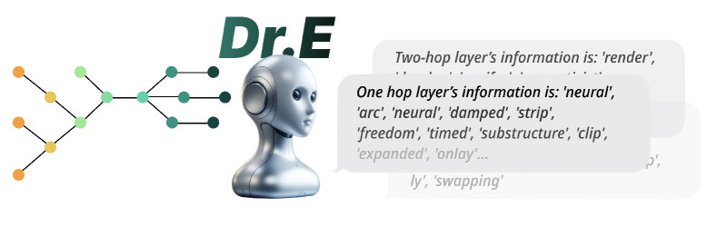
Figure 1: Overview of Dr.E

In this paper, we introduce the Dual-Residual Vector Quantized-Variational AutoEncoder (Dr.E), our ‘graph language’ translator designed to seamlessly map graph data to LLM-compatible tokens and subsequently decode these tokens back into their original graph structures. This approach also addresses the limitations of existing GNN methods, which lack general knowledge and often lose crucial information during the iterative message-passing process. Detailed architecture of Dr.E can be found in  3. To validate the robustness of our proposed method, we evaluated Dr.E’s superior graph data modeling capabilities compared to the baselines, not only on classical node representation tasks but also on few-shot tasks on graphs, demonstrating its excellent generalization performance.

The main contributions of our work are summarized as follows:

• Dr.E represents the first and a pioneering effort to achieve token-level alignment between GNNs and LLMs, setting a new standard for the integration of graph data in multi-modal learning environments.

• By implementing intra-layer and inter-layer residuals, we ensure the preservation of multi-layer perspectives at each convolution step, allowing for robust information transmission from the surrounding nodes to the center.

• We evaluate Dr.E on node classification tasks, where it notably surpasses most GNN-based and LLM-based methods under both fine-tuning and few-shot scenarios, demonstrating the effectiveness of our approach.

2 Background

We mainly introduce the key research directions discussed in the Introduction section and highlight some representative works within these areas, i.e., Vector Quantized Variational AutoTokenizer, Integration of Large Language Model and Graph Neural Network, and Few-shot Learning on Graphs.

2.1 Vector Quantized Variational AutoTokenizer

Among research of modality fusion in computer vision, Vector Quantized-Variational AutoEncoder (VQ-VAE) [25] emerges as an appropriate architectural choice as it trained a discrete codebook that closely resembles the structure of LLMs’ token embeddings. Leveraging the latent expressive capabilities of the codebook in VQ-VAE, endeavors have been directed toward aligning visual tokens with LLMs’ vocabulary. LQAE [14] employed the RoBERTa-augmented VQ-VAE model on few-shot settings, after which the CLIP [17] model has been utilized to augment visual and textual alignment in SPAE [35] and V2L-tokenizer [38].

However, despite these advancements in aligning visual and textual modalities, there has not been a pretrained language-graph contrastive model as CLIP given the uniqueness of graph-structured data. However, since VQ-VAE architecture was first proposed, various refined versions have been developed [19]. Particularly within the domain of GNNs, VQ-VAE has been adapted to facilitate distillation from GNNs to Multilayer Perceptrons (MLPs) [31]. TIGER [18] has employed a residual approach to conduct sequential generative retrieval drawing from the experience of RQ-VAE [11], as we will also apply in our quantizing process to enhance sequential generation and in case of codebook’s collapse.

2.2 Integration of Large Language Model and Graph Neural Network

The integration of GNNs and LLMs has demonstrated significant potential for enhancing model performance across domain-specific tasks [4]. Previous research has established the efficacy of utilizing LLMs as feature-level enhancers, such as in SimTeg [5] and TAPE [8], which delivered frustratingly promising results but limited the full reasoning capabilities of LLMs by relying solely on their pretrained knowledge. Instead of merely utilizing LLMs as annotators, it is more advantageous to engage them as predictors.

An early attempt was to inject the graph embeddings directly into the prompt, thereby enabling LLMs to process node features, a technique employed by InstructGLM [32] through instruction-tuning of the LLM. Later, GraphGPT [22] sought to add new tokens into LLMs vocabulary through a dual-stage tuning process. Furthermore, methods such as LLaGA [3], which avoided fine-tuning the LLM, instead employ a projector to map graph embeddings to token embeddings, subtly encoding graph structural information. In contrast, UniGraph [9] not only trains a graph encoder but also fine-tunes an LLM to execute general GNN tasks using language models. Our research builds upon these methodologies, particularly adopting a similar training procedure as UniGraph to maximize the synergy between graph and language model architectures, thereby unlocking the full potential of this integrated approach.

2.3 Few-shot Learning on Graphs

Given the considerable cost associated with fine-tuning, the concept of few-shot in-context learning emerges as a means to efficiently utilize LLMs. Traditional few-shot learning methods for graph-structured data typically involve learning transferable priors before applying them to similar tasks [6, 26]. However, these approaches are often constrained by requirements such as pretraining on tasks of a similar nature and necessitating uniform input formats. As a response to these limitations, recent research has shifted towards harnessing the inherent capabilities of language models to enable zero-shot or few-shot predictions. For instance, TAG [13] employs raw text alongside pretrained masked language models as input, leveraging the adjacency matrix to learn prior logits for prediction. Similarly, ENG [34] leverages LLMs to generate nodes and edges, thereby expanding the dataset and providing supervision signals, resulting in significant performance improvements.

3 Method

With the goal being infusing the LLMs with knowledge embedded in the graph, the proposed architecture includes two stages of training.

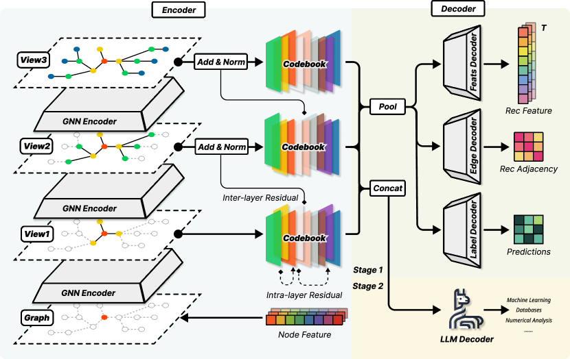
Figure 2: Dual Residual VQ-VAE

Initially, in the first stage, we aim to train Dr.E. This stage involves transforming the node embeddings from the graph into tokens derived from the LLMs’ vocabulary, effectively encoding the contextual information of each node. The Dr.E acts as a pivotal translator within our framework, converting node embeddings into a code that can then be decoded back into node features and graph edges.

In the subsequent second stage, we refine the integration by finetuning the GNN encoder, which is informed by the previous stage, in conjunction with the LLM. This fine-tuning process is conducted in an end-to-end manner, focusing on achieving a fluent translation of the ‘graph’s language’. By structuring our training in this way, we enable the model to leverage the deep semantic understanding of LLMs, thereby enhancing the interpretability and utility of graph data within multi-modal applications.

3.1 Dual-Residual Quantization

During the training of both stages, a subgraph $\mathcal{G}=\left(\mathcal{V},\mathcal{E}\right)$ with node features being $\left\{\mathbf{x}_{v},\forall v\in\mathcal{V}\right\}$ is sampled as described in GraphSage [7], on which we perform both intra-layer and inter-layer residual (i.e., dual-residual) propagation within the encoder of Dr.E.

Codebook

Given a node $v$ with its embedding $\mathbf{h}_{v}$, our goal is to align $\mathbf{h}_{v}$ with the input of LLMs. Within a standard VQ-VAE architecture, a discrete latent variable $\mathbf{e}_{i}$ is selected to represent the observation of a picture (or graph), denoted as $\mathbf{x}$ from a shared codebook by a pair of encoder and decoder, formulated as:

Quantize $(E(\mathbf{x}))=\mathbf{e}_{i},\quad$where $i=\arg\min{{}_{j}}\left\|E(\mathbf{x})-\mathbf{e}_{j}\right\|.$

$E(\mathbf{x})$ denotes the embeddings after non-linear mapping of the input $\mathbf{x}$ by encoder and quantizing process is to find the nearest vector in the codebook. Then the decoder reconstructs the picture (or graph) through another non-linear mapping function. The overall object of standard VQ-VAE is described as:

$$\mathcal{L}(\mathbf{x},D(\mathbf{e}))=\|\mathbf{x}-D(\mathbf{e})\|_{2}^{2}+\|sg[E(\mathbf{x})]-\mathbf{e}\|_{2}^{2}+\beta\|sg[\mathbf{e}]-E(\mathbf{x})\|_{2}^{2},$$

where $\|\mathbf{x}-D(\mathbf{e})\|_{2}^{2}$ is used to update the parameters of the decoder, $\|sg[E(\mathbf{x})]-\mathbf{e}\|_{2}^{2}$ is codebook loss assuring the codes in is close to encoder’s output and $\|sg[\mathbf{e}]-E(\mathbf{x})\|_{2}^{2}$ is commit loss encouraging the encoder generating output close to codes.

In our situation, aiming to select tokens that LLMs are able to read, an intuitive approach involves retrieving the most similar embedding $\mathbf{e}_{C}$ from a codebook $\mathcal{C}$, which can both effectively represent the node and carry semantic meanings. The most straightforward solution is to replace the dynamic codebook from the original VQ-VAE with the token embeddings from LLMs, a method already validated by LQAE [14].

$$\mathcal{C}=\{(c,\mathbf{e}_{c})\mid c\in\mathcal{O}\},$$

where $\mathbf{e}(c)$ denotes the token embedding of index $c$ and $\mathcal{O}$ is the subset of LLMs’ vocabulary. It is worth noting that the tokens chosen by Dr.E do not necessarily convey explainable sentences to humans, but is solely required to be readable to the LLM. However, in order to boost the interpretability of codes selected from the codebook, we preprocess the token and pick out semantically meaningful tokens before transmitting it to the decoder.

Intra-Layer Residual

However, using a single token per layer proves insufficient to capture information embedded within neighboring nodes. To address this, we employ a residual quantization technique to generate codes in sequence. We first select the closest code to the output of the encoder from codebook $\mathcal{C}$, and then subtract the code embedding from the original output to form a new output and iteratively generate new codes, defined as:

$$\mathbf{z}_{v,k}=\arg\min_{\mathbf{e}_{c}}\left\|\mathbf{h}_{v,k-1}-\mathbf{z}_{v,k-1}-\mathbf{e}_{c}\right\|,$$

where $\mathbf{z}_{v,k}$ denotes the embedding after quantized. Subsequently, the update equation for $\mathbf{h}_{v,k}$ is expressed as as:

$$\mathbf{h}_{v,k}=\mathbf{h}_{v,k-1}-\mathbf{z}_{v,k},$$

for $k=1,\ldots,K$, where $k$ means the $k$-th code selected from the codebook and $K$ is number of codes used to quantize a node, while $\mathbf{h}_{v,0}=\mathbf{h}_{v}$ and $\mathbf{z}_{v,0}=\mathbf{0}$. The $K$ codes combined together represent the node $v$, with the intra-layer residual $\mathbf{r}_{v,k}$ at step $k$ being $\mathbf{h}_{v,k}-\mathbf{h}_{v,k-1}$.

Inter-Layer Residual

Instead of using the embedding after aggregating the whole subgraph for downstream tasks, which may lose layer-specific information resulting in insufficient representation on the node, we first extract the central node $v$’s quantized embeddings $\{\mathbf{z}^{t}_{v,k}\}_{k=1}^{K}$ at each convolution step $t$ and save it into the cache. Then we conduct a pooling operation on quantized embeddings and add it onto node embedding before aggregating surrounding nodes $\mathcal{N}(v)$’s embeddings, through which the over-smoothing problem will be alleviated. The forward propagation is defined as:

$$\mathbf{h}^{t+1}_{v}=\sigma\left(\mathbf{W}^{t}\cdot\textsc{CONCAT}\left(\mathbf{h}_{v}^{t}+\textsc{POOL}(\{\mathbf{z}^{t}_{v,k}\}_{k=1}^{K}),\mathbf{h}_{\mathcal{N}(v)}^{t}\right)\right),$$

where $\forall u\in\mathcal{N}(v)$ with $\mathcal{N}(v)$ denoting neighbouring nodes of central node $v$, and $t=1,\dots,T$ with $T$ being number of convolution steps, while $\mathbf{h}_{v}^{0}=\mathbf{x}_{v}$ and $\mathbf{z}_{v,k}^{0}=\mathbf{0}$. The inter-layer residual $\mathbf{r}^{t}_{v}$ at this step is $\mathbf{r}^{t}_{v}=h^{t}_{v}-h^{t-1}_{v}$.

More formally, the embeddings $\mathbf{h}^{t}_{v}$ at step $t$ is an abstraction of embeddings $\mathbf{h}^{t+1}_{v}$ at step $t+1$ as $\mathbf{h}^{t+1}_{v}$ contains information of neighboring nodes one hop farther while sharing the same embedding size of $\mathbf{h}^{t}_{v}$. Also considering multiple layers of views used, fewer codes are needed to represent node $v$, since the representation space is the multiply of codes number at each step $t$:

$$\|\mathcal{E}\|=\|\mathcal{C}\|^{T},$$

where $\|\mathcal{E}\|$ is the representation space of Dr.E’s encoder and $\|\mathcal{C}\|$ is the size of codebook $\mathcal{C}$.

Additionally, the dual-residual generation mirrors the token generation process during LLMs’ inference stage and enhances the representation of sequential information as the newly generated code depends on the previously obtained codes described as:

$$z_{v,k}^{t}=\arg\max_{z_{v,k}^{t}}P\left(z_{v,k}^{t}\mid z_{v,1}^{1},z_{v,2}^{1},\ldots,z_{v,K}^{1},\ldots,z_{v,k-1}^{t}\right)$$

Graph Reconstruction

In terms of the decoder, we fetch the code embeddings $\{\{\mathbf{e}^{t}_{v,k}\}_{k=1}^{K}\}_{t=1}^{T}$ saved from the previous part, pool and direct them into three distinct single-layer linear networks tasked with feature, adjacency and label reconstruction. A simple structured decoder is proven to enhance the expressiveness of the code combinations derived from the codebook and helps in preventing it from collapsing. Mean Squared Error (MSE) Loss and Cross-Entrophy (CE) Loss are employed for feature reconstruction and label prediction. For adjacency reconstruction, considering the sparsity induced by our method of subgraph sampling—where a predefined number of neighbors are selected at each hop—the standard Binary Cross Entropy loss is modified to a Weighted Binary Cross Entropy loss, as also practiced by VGAE, defined as:

$$\mathcal{L}_{adjacency}=-\frac{1}{N}\sum_{i=1}^{N}\left[w_{i}y_{i}\log\left(\hat{y}_{i}\right)+\left(1-y_{i}\right)\log\left(1-\hat{y}_{i}\right)\right],$$

where $N=\left\|\mathcal{V}\right\|^{2}$, representing the total number of possible edges within the graph $\mathcal{G}$, $y_{i},\hat{y}_{1}\in[0,1]$ denoting the ground truth and predictions of whether there exists an edge, $w_{i}=\frac{N}{2*N_{i}}$ is the weight of the $i$-th sample used to adjust its contribution in the loss function, countering the influence of sample imbalance. The overall loss function during the first stage is defined as:

$$\mathcal{L}=\mathcal{L}_{features}+\alpha\mathcal{L}_{labels}+\beta\mathcal{L}_{adjacency},$$

where $\alpha$ and $\beta$ are weighting factors for each corresponding loss component, commit loss in regular VQ-VAE is omitted due to the progressive nature of our quantization process during the generation of new quantized representations.

3.2 Token Alignment Finetuing

During the end-to-end fine-tuning stage, we replace label and edge reconstruction layers with LLM as language decoder. Leveraging Dr.E’s proficiency in translating graphs into tokens, we are able to decode these tokens back into semantically meaningful words and fine-tune the LLM using natural language instructions.

Figure 3: Prompt template for Dr.E’s stage-2 tuning

During the second stage of training, the Dr.E is not frozen but consistently adjusts itself to accommodate the language patterns of the LLM. Throughout this phase, the overall loss function is formulated as follows:

$$\mathcal{L}=\mathcal{L}_{features}+\gamma\mathcal{L}_{LLM}.$$

Here, $\mathcal{L}_{LLM}=-\sum_{i=1}^{N}y_{i}\log(p_{i})$ is a standard cross-entropy loss for language modeling and $\gamma$ denotes the weight attributed to the loss of the LLM decoder.

4 Experiments

To evaluate the efficacy of our framework, Dr.E has been tested on three benchmark datasets—OGBN-Arxiv, PubMed, and Cora—conducting node classification tasks under both fine-tuning and few-shot transfer scenarios. Each of these datasets is a citation network, where the task involves predicting the category label of a target node.

More specifically, we fine-tune our model on these three datasets to fully harness the capabilities of Dr.E. Additionally, we explore the model’s generalizability by pretraining the encoder on OGBN-Arxiv, the largest of the three datasets, to align nodes with textual tokens, followed by making few-shot predictions on PubMed and Cora. It is also important to note that while Dr.E is adept at handling Text-Attributed Graphs (TAG), it can also be generalized to non-textual graphs. However, our study focuses on these particular datasets due to their data availability.

4.1 Experiment Settings

To enhance the reproducibility of our experiments and ensure fair comparison with prior work, we employ the LLaMA-2-7B as our LLM decoder, which is also widely used in various other studies. Consequently, we exclude comparisons with studies utilizing variants of LLaMA or other LLMs as foundational models, despite acknowledging the novelty and effectiveness of approaches like InstructGLM [32], GraphGPT [22], LLaGA [23] and so on.

Dr.E incorporates three graph convolution layers as an encoder to obtain three-layer perspectives when encoding a node into tokens. We incorporate an activation function and a quantizing module following dropout regularization to prevent zero values from populating the embeddings. The convolution blocks are uniform and can be scaled to stack multiple times. Cosine similarity is employed to identify the nearest token, which has proven to outperform a language model (LM) head layer in terms of convergence speed.

We implement LoRA PEFT for LLaMA-2 and establish two independent learning rates for the GNN encoder and LLM decoder, set at 1e-3 and 5e-5, respectively, with a weight decay of 5e-4. The hidden dimension for the GCN is 4096, matching the token embedding dimension of LLaMA, and 8 codes are selected to represent each layer’s view. We significantly increase the weight for feature reconstruction loss by 100 times to more accurately restore the nodes’ features, while maintaining edge and label reconstruction loss as a weak supervised signal.

Our experiments are conducted on multiple NVIDIA A800-SXM4-80GB GPUs.

4.2 Main Evalution

This section employs accuracy as the primary metric for node classification unless otherwise noted.

Fine-tuning

We compare Dr.E with classic GNN-based models, transformer-based graph learners, and other combined LLM-GNN methods. The results represent the average score from five runs with different random seeds. The highest score for each dataset is highlighted in bold.

Table 1: Dr.E achieves better score than classic GNN models and various latest frameworks

Datasets	MLP	GCN	GAT	CoarFormer	Graphormer	UniGraph	Dr.E
Arxiv	0.5011	0.7252	0.7366	0.7291	0.7166	0.7281	0.7578
Pubmed	0.6199	0.8890	0.8328	0.7433	0.8975	0.8041	0.9462
Cora	0.5012	0.8778	0.7670	0.8143	0.8869	0.8824	0.8934
Average	0.5407	0.8307	0.7788	0.7622	0.8337	0.8049	0.8658

From Table LABEL:fine-tuned, Dr.E consistently outperforms most GNN models. However, it does incur a higher training cost; stage-2 tuning of Dr.E averages 16 GPU hours on the OGBN-Arxiv dataset, with batch size and gradient accumulation steps set at 4 and 8, respectively. Moreover, Dr.E scores higher than combined GNN-LLM methods like UniGraph, even though the tuning of LLM for Dr.E requires fewer tokens, as we do not provide detailed textual descriptions of the nodes. Overall, Dr.E demonstrates its potential to surpass classical methods in specific tasks and remains competitive with contemporary frameworks.

Few-shot Transfer

We conduct few-shot transfer experiments on the Cora and PubMed datasets after pretraining Dr.E’s encoder on OGBN-Arxiv. Since few-shot settings differ significantly between LLM predictors and traditional few-shot GNN models, we primarily compare our method with LLaMA, while also including heuristic GNN-methods for a more comprehensive comparison.

Table 2: Few-shot transfer on Pubmed dataset.

Methods	0-shot	1-shot	2-shot	3-shot	4-shot	5-shot	Average
GCN	-	0.6052	0.6316	0.6322	0.6558	0.7526	0.6555
GAT	-	0.5972	0.6348	0.6376	0.6588	0.6692	0.6395
DGI	-	0.6488	0.6470	0.6988	0.7098	0.7376	0.6884
MVGRL	-	0.6178	0.6470	0.6542	0.6936	0.6958	0.6617
GRACE	-	0.6380	0.6770	0.6874	0.6960	0.7146	0.6826
Meta-PN	-	0.5752	0.5956	0.6660	0.6952	0.6966	0.6457
CGPN	-	0.5903	0.5690	0.6300	0.6503	0.6473	0.6174
LLaMA-2-7B	0.1731	0.3879	0.4173	0.4798	0.5074	0.6022	0.4280
Dr.E	0.3269	0.3846	0.5288	0.6731	0.7015	0.7199	0.5558

Table 3: Few-shot transfer on Cora dataset.

Methods	0-shot	1-shot	2-shot	3-shot	4-shot	5-shot	Average
GCN	-	0.6032	0.6486	0.6830	0.7194	0.7574	0.6823
GAT	-	0.5176	0.5590	0.6116	0.6774	0.7126	0.6156
DGI	-	0.6206	0.7126	0.7296	0.7688	0.7842	0.7232
MVGRL	-	0.6290	0.6850	0.7208	0.7544	0.7860	0.7150
GRACE	-	0.6700	0.6878	0.7320	0.7536	0.7768	0.7240
Meta-PN	-	0.5920	0.6892	0.7530	0.7650	0.7710	0.7140
CGPN	-	0.6794	0.7346	0.7576	0.7570	0.7746	0.7406
LLaMA-2-7B	0.2629	0.4023	0.4482	0.4982	0.5343	0.6031	0.4581
Dr.E	0.3892	0.4813	0.6192	0.6975	0.7108	0.7420	0.6066

Under the transfer setting in Table LABEL:few-shot, Dr.E outperforms the vanilla version of LLaMA-2, suggesting that LLMs are capable of learning language patterns within the prompt and making predictions based on examples provided in context, even though the information encoded by Dr.E is not directly interpretable.

4.3 Model Analysis

Ablation Study

To validate the efficacy of Dr.E, we initially deactivate its encoder and fine-tune the LLaMA-2-7B directly with raw text. This step aims to demonstrate that our token selection by Dr.E incorporates graph structure-related information, consequently improving the performance of the LLM decoder. Additionally, we isolate and analyze the contributions of the multi-layer view, intra-layer, and inter-layer residuals within Dr.E.

Table 4: Ablation studies on Dr.E, with node classification accuracy is evaluated on three datasets. ’+’ denotes module added to the previous stage. ’Token Refinement’ process denotes selecting meaningful embeddings of words to replace the frozen codebook.

Method	Arxiv	Pubmed	Cora
LLaMA-2-7B	0.5319	0.1731	0.2629
LLaMA-2-7B + LoRA	0.6524	0.8213	0.8012
+ Base VQ with frozen codebook	0.6612	0.8124	0.7921
+ Inter-layer Residual	0.6901	0.8712	0.8422
+ Intra-layer Residual	0.7023	0.9012	0.8512
+ Pretraining Encoder	0.7432	0.9415	0.8890
+ Token Refinement	0.7578	0.9462	0.8934

It is evident from Table LABEL:ablation that the dual-residual design consistently enhances the overall performance. Furthermore, token refinement not only sustains the performance of Dr.E but also significantly enhances the interpretability of the selected tokens.

Token Selection

To assess the effective utilization of the codebook during the encoding process, we calculate perplexity, defined as the exponential of the negative entropy of the code distribution. This measure helps indicate how well the latent space is being used, which can be a critical factor for model performance. The formula for perplexity is given by:

$$\textsc{Perplexity}=\exp\left(-\sum_{i=1}^{\|\mathcal{C}\|}p_{i}\log p_{i}\right),$$

where $\|\mathcal{C}\|$ represents the total number of codes in the codebook, and $p_{i}$ denotes the probability of the $i$-th code being used, typically estimated by the relative frequency of each code in the dataset.

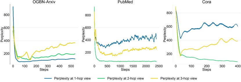
Figure 4: Perplexity at each dataset. Please Note that we apply Savitzky-Golay filter [20] when drawing line-graph for better readability. ’x-hop’ denotes neighboring nodes at x-hop away from central node.

During the training process, the perplexity for each layer’s view initially decreases to a minimal amount before rebounding to reasonable values. Additionally, the perplexities across the three layers follow a ratio of 1:2:3, suggesting that the amount of information aggregated increases as it propagates through the layers.

We also conduct visual analysis of the words selected by Dr.E, which reveals that not all words carry label-related information, though collectively, they contribute to the final prediction, as can be seen in Figure 5.

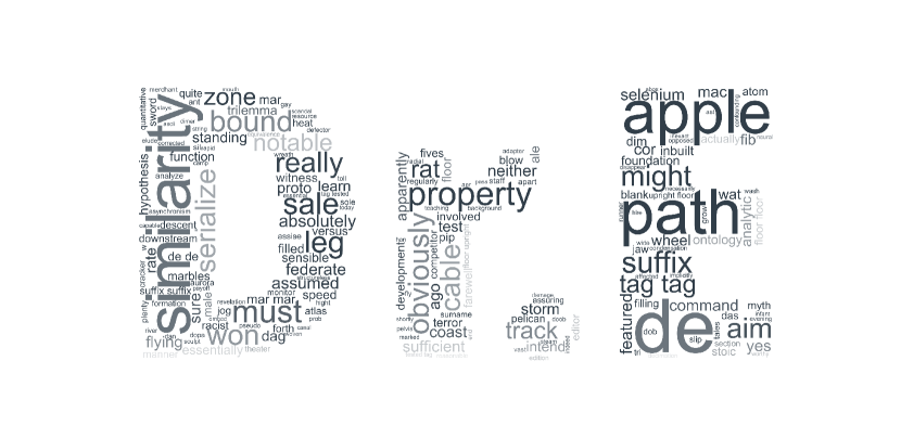
Figure 5: Word cloud of Dr.E, partly selected from Arxiv training dataset. Larger words in the word cloud represent more frequently occurring terms in the source material. Words like "serialize," "sale," "bound," and "path" appear prominently, which might indicate their importance to the central nodes.

5 Conclusion

In this study, we introduce an end-to-end framework that seamlessly integrates graph-structured data with Large Language Models (LLMs). Our framework, leveraging graph-structured information through both intra-layer and inter-layer residuals, employs a Dual-Residual Vector Quantized-Variational AutoEncoder (Dr.E). This innovative approach effectively bridges the gap between Graph Neural Networks (GNNs) and LLMs, enabling the translation of graph data into natural language at the token level while preserving semantic and structural integrity.

Dr.E exhibits superior performance in GNN node classification tasks, demonstrating robustness and efficiency in both fine-tuning and few-shot scenarios. Nevertheless, the challenge of handling extremely large and complex graphs persists. Future endeavors may explore advanced tokenization techniques and scalable training methods to further enhance performance.

References

- [1] Josh Achiam, Steven Adler, Sandhini Agarwal, Lama Ahmad, Ilge Akkaya, Florencia Leoni Aleman, Diogo Almeida, Janko Altenschmidt, Sam Altman, Shyamal Anadkat, et al. Gpt-4 technical report. arXiv preprint arXiv:2303.08774, 2023.
- [2] Tom Brown, Benjamin Mann, Nick Ryder, Melanie Subbiah, Jared D Kaplan, Prafulla Dhariwal, Arvind Neelakantan, Pranav Shyam, Girish Sastry, Amanda Askell, et al. Language models are few-shot learners. Advances in neural information processing systems, 33:1877–1901, 2020.
- [3] Runjin Chen, Tong Zhao, Ajay Jaiswal, Neil Shah, and Zhangyang Wang. Llaga: Large language and graph assistant. arXiv preprint arXiv:2402.08170, 2024.
- [4] Zhikai Chen, Haitao Mao, Hang Li, Wei Jin, Hongzhi Wen, Xiaochi Wei, Shuaiqiang Wang, Dawei Yin, Wenqi Fan, Hui Liu, et al. Exploring the potential of large language models (llms) in learning on graphs. ACM SIGKDD Explorations Newsletter, 25(2):42–61, 2024.
- [5] Keyu Duan, Qian Liu, Tat-Seng Chua, Shuicheng Yan, Wei Tsang Ooi, Qizhe Xie, and Junxian He. Simteg: A frustratingly simple approach improves textual graph learning. arXiv preprint arXiv:2308.02565, 2023.
- [6] Victor Garcia and Joan Bruna. Few-shot learning with graph neural networks. arXiv preprint arXiv:1711.04043, 2017.
- [7] Will Hamilton, Zhitao Ying, and Jure Leskovec. Inductive representation learning on large graphs. Advances in neural information processing systems, 30, 2017.
- [8] Xiaoxin He, Xavier Bresson, Thomas Laurent, Adam Perold, Yann LeCun, and Bryan Hooi. Harnessing explanations: Llm-to-lm interpreter for enhanced text-attributed graph representation learning, 2023.
- [9] Yufei He and Bryan Hooi. Unigraph: Learning a cross-domain graph foundation model from natural language. arXiv preprint arXiv:2402.13630, 2024.
- [10] Thomas N Kipf and Max Welling. Semi-supervised classification with graph convolutional networks. arXiv preprint arXiv:1609.02907, 2016.
- [11] Doyup Lee, Chiheon Kim, Saehoon Kim, Minsu Cho, and Wook-Shin Han. Autoregressive image generation using residual quantization. In Proceedings of the IEEE/CVF Conference on Computer Vision and Pattern Recognition, pages 11523–11532, 2022.
- [12] Xin Li, Dongze Lian, Zhihe Lu, Jiawang Bai, Zhibo Chen, and Xinchao Wang. Graphadapter: Tuning vision-language models with dual knowledge graph. Advances in Neural Information Processing Systems, 36, 2024.
- [13] Yuexin Li and Bryan Hooi. Prompt-based zero-and few-shot node classification: A multimodal approach. arXiv preprint arXiv:2307.11572, 2023.
- [14] Hao Liu, Wilson Yan, and Pieter Abbeel. Language quantized autoencoders: Towards unsupervised text-image alignment. Advances in Neural Information Processing Systems, 36, 2024.
- [15] Andrew Kachites McCallum, Kamal Nigam, Jason Rennie, and Kristie Seymore. Automating the construction of internet portals with machine learning. Information Retrieval, 3:127–163, 2000.
- [16] Arnold K Nyamabo, Hui Yu, and Jian-Yu Shi. Ssi–ddi: substructure–substructure interactions for drug–drug interaction prediction. Briefings in Bioinformatics, 22(6):bbab133, 2021.
- [17] Alec Radford, Jong Wook Kim, Chris Hallacy, Aditya Ramesh, Gabriel Goh, Sandhini Agarwal, Girish Sastry, Amanda Askell, Pamela Mishkin, Jack Clark, et al. Learning transferable visual models from natural language supervision. In International conference on machine learning, pages 8748–8763. PMLR, 2021.
- [18] Shashank Rajput, Nikhil Mehta, Anima Singh, Raghunandan Hulikal Keshavan, Trung Vu, Lukasz Heldt, Lichan Hong, Yi Tay, Vinh Tran, Jonah Samost, et al. Recommender systems with generative retrieval. Advances in Neural Information Processing Systems, 36, 2024.
- [19] Ali Razavi, Aaron Van den Oord, and Oriol Vinyals. Generating diverse high-fidelity images with vq-vae-2. Advances in neural information processing systems, 32, 2019.
- [20] Ronald W Schafer. What is a savitzky-golay filter?[lecture notes]. IEEE Signal processing magazine, 28(4):111–117, 2011.
- [21] Frank Spitzer. Principles of random walk, volume 34. Springer Science & Business Media, 2001.
- [22] Jiabin Tang, Yuhao Yang, Wei Wei, Lei Shi, Lixin Su, Suqi Cheng, Dawei Yin, and Chao Huang. Graphgpt: Graph instruction tuning for large language models. arXiv preprint arXiv:2310.13023, 2023.
- [23] Hugo Touvron, Louis Martin, Kevin Stone, Peter Albert, Amjad Almahairi, Yasmine Babaei, Nikolay Bashlykov, Soumya Batra, Prajjwal Bhargava, Shruti Bhosale, et al. Llama 2: Open foundation and fine-tuned chat models. arXiv preprint arXiv:2307.09288, 2023.
- [24] Maria Tsimpoukelli, Jacob L Menick, Serkan Cabi, SM Eslami, Oriol Vinyals, and Felix Hill. Multimodal few-shot learning with frozen language models. Advances in Neural Information Processing Systems, 34:200–212, 2021.
- [25] Aaron Van Den Oord, Oriol Vinyals, et al. Neural discrete representation learning. Advances in neural information processing systems, 30, 2017.
- [26] Song Wang, Kaize Ding, Chuxu Zhang, Chen Chen, and Jundong Li. Task-adaptive few-shot node classification. In Proceedings of the 28th ACM SIGKDD Conference on Knowledge Discovery and Data Mining, pages 1910–1919, 2022.
- [27] Likang Wu, Zhaopeng Qiu, Zhi Zheng, Hengshu Zhu, and Enhong Chen. Exploring large language model for graph data understanding in online job recommendations. In Proceedings of the AAAI Conference on Artificial Intelligence, volume 38, pages 9178–9186, 2024.
- [28] Likang Wu, Hongke Zhao, Zhi Li, Zhenya Huang, Qi Liu, and Enhong Chen. Learning the explainable semantic relations via unified graph topic-disentangled neural networks. ACM Transactions on Knowledge Discovery from Data, 17(8):1–23, 2023.
- [29] Likang Wu, Zhi Zheng, Zhaopeng Qiu, Hao Wang, Hongchao Gu, Tingjia Shen, Chuan Qin, Chen Zhu, Hengshu Zhu, Qi Liu, et al. A survey on large language models for recommendation. arXiv preprint arXiv:2305.19860, 2023.
- [30] Zonghan Wu, Shirui Pan, Fengwen Chen, Guodong Long, Chengqi Zhang, and S Yu Philip. A comprehensive survey on graph neural networks. IEEE transactions on neural networks and learning systems, 32(1):4–24, 2020.
- [31] Ling Yang, Ye Tian, Minkai Xu, Zhongyi Liu, Shenda Hong, Wei Qu, Wentao Zhang, CUI Bin, Muhan Zhang, and Jure Leskovec. Vqgraph: Rethinking graph representation space for bridging gnns and mlps. In The Twelfth International Conference on Learning Representations, 2023.
- [32] Ruosong Ye, Caiqi Zhang, Runhui Wang, Shuyuan Xu, and Yongfeng Zhang. Natural language is all a graph needs. arXiv preprint arXiv:2308.07134, 2023.
- [33] Jiahui Yu, Yuanzhong Xu, Jing Yu Koh, Thang Luong, Gunjan Baid, Zirui Wang, Vijay Vasudevan, Alexander Ku, Yinfei Yang, Burcu Karagol Ayan, et al. Scaling autoregressive models for content-rich text-to-image generation. arXiv preprint arXiv:2206.10789, 2(3):5, 2022.
- [34] Jianxiang Yu, Yuxiang Ren, Chenghua Gong, Jiaqi Tan, Xiang Li, and Xuecang Zhang. Empower text-attributed graphs learning with large language models (llms). arXiv preprint arXiv:2310.09872, 2023.
- [35] Lijun Yu, Yong Cheng, Zhiruo Wang, Vivek Kumar, Wolfgang Macherey, Yanping Huang, David Ross, Irfan Essa, Yonatan Bisk, Ming-Hsuan Yang, et al. Spae: Semantic pyramid autoencoder for multimodal generation with frozen llms. Advances in Neural Information Processing Systems, 36, 2024.
- [36] Jianan Zhao, Le Zhuo, Yikang Shen, Meng Qu, Kai Liu, Michael Bronstein, Zhaocheng Zhu, and Jian Tang. Graphtext: Graph reasoning in text space. arXiv preprint arXiv:2310.01089, 2023.
- [37] Jie Zhou, Ganqu Cui, Shengding Hu, Zhengyan Zhang, Cheng Yang, Zhiyuan Liu, Lifeng Wang, Changcheng Li, and Maosong Sun. Graph neural networks: A review of methods and applications. AI open, 1:57–81, 2020.
- [38] Lei Zhu, Fangyun Wei, and Yanye Lu. Beyond text: Frozen large language models in visual signal comprehension. arXiv preprint arXiv:2403.07874, 2024.