Emergent Complexity in the Decision-Making Process of Chess Players

Abstract

In this article, we study the decision-making process of chess players by using a chess engine to evaluate the moves across different pools of games. We quantify the decisiveness of each move during the games using a metric called $\Delta$, which is derived from the engine’s evaluation of the positions. We then performed a comparative analysis across players of varying competitive levels. Firstly, we observed that players face a wide spectrum of $\Delta$ values, evidencing the complexity of the process. By examining groups of winning and losing players, we found evidence where a decrease in complexity may be associated with a drop in player performance levels. Secondly, we observed that players’ accuracy increases in positions with high $\Delta$ values regardless of competitive level. Complementing this information with a null model where players make completely random legal moves allowed us to characterize the decision-making process under the simple strategy of making moves that minimize $\Delta$ values. Finally, based on this idea, we proposed a simple model that approximately replicates the global emergent properties of the system.

I Introduction

Within the framework of complexity science, a sports competition can be thought of as a complex system whose dynamics evolve based on interactions of cooperation and competition, modulating players’ behavior in response to highly changing environments. This inherently complex nature, characteristic of sports competitions, has historically captivated the interest of academics. In recent years, the remarkable advancements in dynamic data acquisition capabilities, combined with increased computational power, have amplified this natural interest, prompting the emergence of several multidisciplinary studies aimed at analyzing the emergent properties of these systems [1, 2, 3, 4, 5, 6, 7]. In this context, we have previously analyzed sports such as football [8, 9, 10], volleyball [11], and paddle tennis [12]. With the same spirit, this study focuses on the game of chess.

Chess has accompanied mankind’s history from ancient times [13], in the last century it was a benchmark for the evolution of computers [14], and in recent times it boosted developments of the artificial intelligence [15]. The utilities of chess go beyond as it is also useful for testing different human capabilities. To mention a few applications, this game has been used to evaluate cognitive performance in professional and novice players [16], decision making processes [17, 18], the relation between expertise and knowledge [19, 20] and gap gender [21]. What makes chess such a useful tool lies in two pillars, namely, complexity and popularity.

Features of complexity were measured in the last years, analyzing the collective behavior of a pool of chess players using extensive databases [22, 23, 24, 25, 26, 27, 28, 29, 30]. Blasius and Tönjes [22] reported a Zipf’s law behavior for the pooled distribution of chess opening weights and these findings were explained analytically as a multiplicative process. Studying the growing dynamics of the game tree, we have found that the emerging Zipf and Heaps laws can be explained in terms of nested Yule-Simon preferential growth processes [24]. Also, we have observed long-range memory effects in time-stamped registered games [25, 27] and correlations between communities of players and their level of expertise [28]. Atashpendar et al. [26] have analyzed the structure of the state space of chess. They concluded that this space consists of several pockets between which transitions are rare, and that skilled players sparsely explore some these pockets. De Marzo and Servedio [29] applied the Economic Fitness and Complexity algorithm to measure the difficulty of openings and players’ skill levels. Ribeiro et al. [23] investigated the move-by-move dynamics of the white player’s advantage finding that the diffusion of the move dependence of the White player’s advantage is non-Gaussian, has long-ranged anti-correlations and that it becomes super-diffusive after an initial period with no diffusion. Recently, Barthelemy [30] have used Stockfish to search critical points [31], performing a statistical analysis of the difference between the evaluations of the best move and the second best move introducing the parameter $\Delta$.

Nowadays, the popularity of chess encompasses big active communities of players including all levels of expertise. Matches occur in both the traditional over-the-board way and online portals. These vast worldwide communities of chess players produce extensive game records, providing a big source of data for large-scale analyses. In these databases, the expertise of each player is statistically well characterized through the ‘Elo’ system introduced by the physicist Arpad Elo [32]. This rating system is also predictive since it permits to anticipate the result of one match between two ranked players.

In this research paper, we first review and check results on the statistics of chess play reported in the literature [22, 30], while introducing new observables reported here for the first time. In particular, we introduce a null reference model to determine specific game-level characteristics. These results allow us to establish a framework for developing a statistical model for matches of the game. The model is based on microscopic mechanisms of the players’ decision-making as the game unfolds. This allows us to understand the emergence of various macroscopic statistics of the system. To establish this mechanism, we carried out a data drive analysis of chess games based on the StockFish chess engine. The engine allows us to quantify how much the players’ decisions affect the development of the game.

The manuscript is divided into five sections: in the section following this introduction, Section II, we describe the datasets used and provide details of the acquisition process. In Section III, we present various results from our analysis. Finally, in the last section, we briefly summarize the main conclusions of the paper.

II Data

In this paper, we analyze three public datasets, with the aim of conducting an analysis based on the competitive level of the players. The first dataset, referred to as FIDE, contains $3000$ games from the World Championships and European Championships from the years 2019, 2020, 2021, and 2022. These games are of a high competitive level. The second dataset, referred to as LC high ELO, contains $1000$ games played by players on the Lichess platform [33] where the average rating between the two competitors is above 2500. The rating used here is the one assigned by the Lichess portal, calculated based on the player’s game history on that platform. The games collected in this dataset correspond to an intermediate competitive level. Finally, the dataset referred to as LC low ELO contains $3000$ games played by players on the Lichess platform where the average rating between competitors is below 1500. These games are from beginner players, with a low competitive level. All datasets contains classical chess games in portable game notation (pgn) format. The games associated with the FIDE dataset were downloaded from the website The Week in Chess [34], and the others from the Lichess database [35].

III Results and discussion

III.1 Global emergents in chess

When a chess player faces a position on the board, they must evaluate it, decide which move is most advantageous, and execute it. This decision-making process is based on the game’s tactical and strategic principles, which, like in any sport, the player acquires and refines during their training. A chess game, therefore, can be thought of as a succession of positions that both players must evaluate accurately until the end of the game. In each of these positions, a finite number of legal moves, $\mu$, define the range of possible plays for the competitor. Since $\mu$ is a finite random variable, the evolution of the game can be represented as a walk in a vast and complex decision tree.

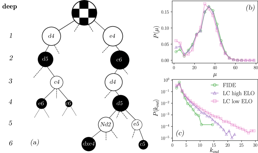
Figure 1: The Chess Tree. (a) Schematic of a small portion of the chess tree. Each node represents a board position, with the label indicating the last move made. The size of the nodes (not to scale) indicates that some nodes are more popular than others. (b) At each turn, depending on the stage of the game, players have a certain number of legal moves, $\mu$. The plot shows the distribution $P(\mu)$. (c) The empirical tree, constructed from the data, can be thought of as a directed complex network, where the nodes have $k_{out}$ outgoing links. The plot shows the distribution $P(k_{out})$.

In Fig. 1 (a), we show a small region of the decision tree, highlighting the first moves of the Queen’s Gambit opening (left) and the Caro-Kann Defense (right). From now on, we will refer to the number of moves as depth, $d$, referring to the depth of the tree. The size of the circles in the graph is proportional to the popularity of each node, that is, the number of times, $n$, that position was observed in the database. In Fig. 1 (b), we show the distribution $P(\mu)$. We calculated the mean value and the standard deviation in the three cases and obtained similar results, $\left\langle\mu\right\rangle\approx 30$ and $\sigma_{\mu}\approx 12$. We can see that the distribution shows an approximately normal behavior with a large peak around $\mu\approx 35$ and a smaller peak around $\mu\approx 5$. The latter is associated with check situations, where legal moves are reduced. Note that lower-level players seem to be more exposed to these situations. Notably, these results are similar to those reported in [30] for the case of engine chess games, indicating that the approximately normal shape of $P(\mu)$ is something intrinsic to the game. Lastly, we constructed a directed network with nodes that meet $n>1$ and studied the degree distribution, $P(k)$, which we show in Fig. 1 (c). We call this network the empirical tree because it is formed only by the nodes that appear in the database. In all three cases, we observed curves with a sample mean of $\left\langle k\right\rangle\approx 1$. This indicates that the tree is mainly formed by chains. Interestingly, the variance decreases as the level of the players increases. Higher-level players tend to explore fewer variants compared to lower-level players, probably because they have a greater ability to decide primarily on good lines.

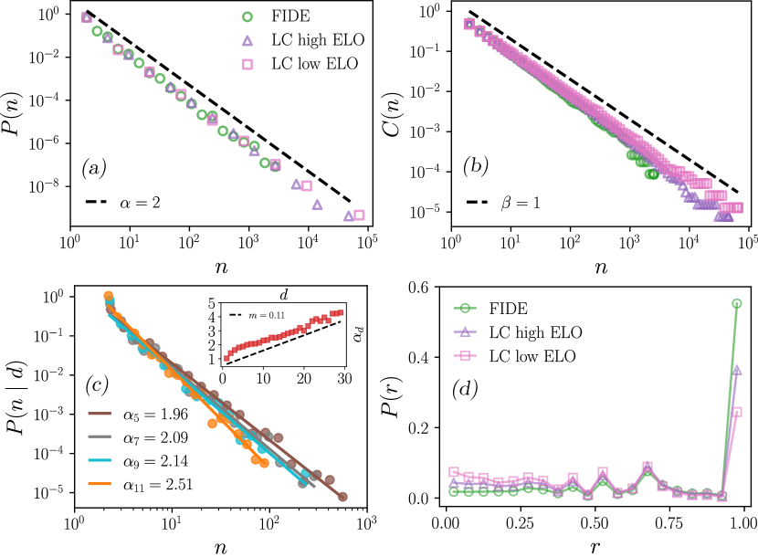
Figure 2: Global Emergent Properties of the System. (a) Distribution of node popularity, $P(n)$, in the three datasets analyzed: FIDE, LC high ELO, and LC low ELO. Dashed lines show the theoretical distribution $P(n)=n^{-2}$. (b) Complementary cumulative distribution of node popularity, $C(n)$, in the three datasets analyzed. Dashed lines show the theoretical distribution $C(n)=n^{-1}$ (Zipf’s law). (c) Conditional popularity distribution at a specific tree depth, $P(n|d)$. Solid lines show a nonlinear fit to the curves used to calculate the exponents $\alpha_{d}$. The inset shows the relationship between $\alpha_{d}$ and depth $d$. (d) Distribution of ratios, $P(r)$, for the three datasets analyzed.

In Fig. 2 (a) and (b), we show the distribution of node popularity, $P(n)$, and the complementary cumulative distribution, $C(n)=1-P(N\leq n)$. It is well known that the game tree is self-similar and $C(n)$ follows Zipf’s law [22]. In dashed lines, we show $P(n)\propto n^{-\alpha}$, and $C(n)\propto n^{-\beta}$, with $\alpha=2$ and $\beta=1$. Notably, the distributions do not appear to depend on the competitive level of the players. By collecting $N=10^{4}$ random games from the three datasets, we measured the node popularity at different depth levels to obtain $P(n|d)$. In Fig. 2 (c), we can see that these distributions also follow a power law, $P(n|d)\propto n^{-\alpha_{d}}$. Likewise, the exponents $\alpha_{d}$ follow a linear trend as a function of depth, as shown in the inset of the figure. This trend can be estimated as $m=1/\log(N)\approx 0.11$ [22]. The dashed lines show how the theoretical line, $\alpha_{d}\propto m\times d$, closely approximates the empirical trend.

Finally, we define the branching ratio, $r$, as follows: Let $i$ and $j$ be two connected nodes in the network located at levels $d$ and $d+1$. Let $n^{i}_{d}$ and $n^{j}_{d+1}$ be the popularities of these nodes, then $r^{ij}=n^{j}_{d+1}/n^{i}_{d}$. Note that when $r^{ij}=1$, all players who passed through node $i$ chose the same move that leads to node $j$. Conversely, when $r^{ij}\approx 0$, few players who passed through node $i$ chose the move leading to node $j$. In Fig. 2 (d), we show the distribution $P(r)$ for the three analyzed datasets. To calculate $r^{ij}$ for each pair of nodes, we require that $n^{j}_{d}>1$ and $n^{j}_{d+1}>1$. We can see the presence of a peak around $r\approx 1$. For the rest of the range, the distribution approximates a uniform distribution. These observations coincide with those reported in [22]. It is also observed that an increase in the competitive level of the players produces a larger peak around $r\approx 1$ and a lower values in the distribution for $r<0.5$. This is consistent with what is observed in Fig. 1 (c), where lower-level players tend to explore more paths than higher-level players.

III.2 Quantifying the Spectrum of Decisions

During the game, players must evaluate different types of positions to decide which is the best move to make. A natural question is whether all decisions have the same impact on the game. In this section, we discuss this issue.

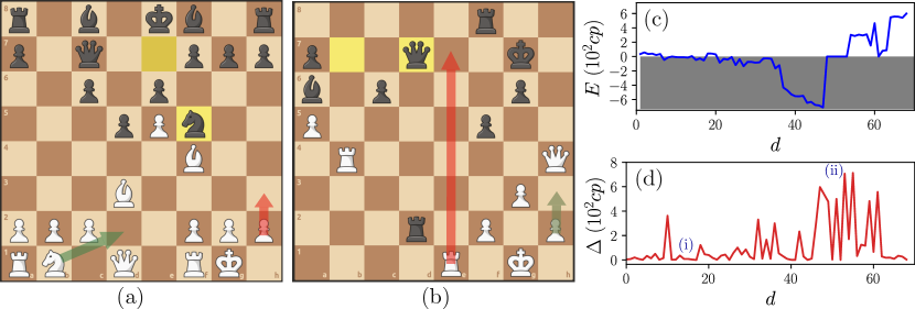
Figure 3: Evaluation and Quantification of Decisions. (a) Example of a position where the decision of the moving player (White) is not very decisive for the game. (b) Example of a position where the decision is decisive for the game. (c) StockFish evaluation of an anonymous game from the LC low ELO dataset. (d) Value of $\Delta$ at each position in the game mentioned in the previous panel. References (i) and (ii) indicate the moments in the game where the positions shown in panels (a) and (b) appear.

To quantify the players’ decisions, we used one of the best chess engines available today: StockFish 16 (SF) [36]. For our study, SF was configured to work with an ELO rating of 3500 and an analysis depth of 20 moves. Given a position, SF evaluates it and quantifies its evaluation with a number we call $E$. In Fig. 3 (c), we show the evaluation curve of all positions in a game, $E$ vs. $d$. In this scheme, if $E\approx 0$, SF indicates that the game is even. If $E>0$ ($E<0$) the advantage is for the player with the White (Black) pieces. The values of $E$ are given in units of centipawns, $[E]=cp$, where each unit represents 1/100 of a pawn advantage.

Given a position, SF also allows us to rank all possible moves, from best to worst, based on the evaluation it would give to the resulting position if we made that move. In Fig. 3 (a) and (b), we show two positions from a game, both with White to move. In each case, we used SF to obtain the top three moves (M). For the position in panel (a), we have: (1) $M_{1}=h3$ with $E_{1}=+0.37$, (2) $M_{2}=\symknight d2$ with $E_{2}=+0.37$, and (3) $M_{3}=\symrook e1$ with $E_{3}=+0.35$. For the position in panel (b), we obtain: (1) $M_{1}=\symrook e7$ with $E_{1}=+2.96$, (2) $M_{2}=h3$ with $E_{2}=-4.11$, and (3) $M_{3}=\symrook bb1$ with $E_{3}=-4.46$. All $E$ values are expressed in $10^{2}cp$.

Note that in the case of the position in panel (a), the decision the player makes doesn’t seem to matter much. Any of the three moves SF suggested results in a similar evaluation of the game. We say that this type of position is “not very decisive” because a bad decision cannot significantly alter the course of the game. Of course, we are talking about rational decisions, excluding irrational moves like $\symbishop h6$, a move that sacrifices a bishop for no reason. Conversely, in the position in panel (b), it is very important that the player makes the correct move. In this position, if White plays $M_{1}=\symrook e7$, it executes a fork, attacking both the king and queen with the rook simultaneously. Being in check, the black king must move, and White will capture the black queen, which gives a decisive advantage. Note that only $M_{1}$ gives an advantage to the player with White; any other option will put them at a disadvantage. We say that this type of position is “highly decisive” because a bad decision can change the course of the game.

To quantify how decisive the position the players are facing is, previous works have proposed measuring the parameter $\Delta=|E_{1}-E_{2}|$ [30]. Note that if $\Delta$ is small, it indicates a less decisive position, and if $\Delta$ is large, it indicates a highly decisive position, such as those shown in Fig. 3 (a) and (b), respectively. In particular, if $\Delta>\left\langle\Delta\right\rangle$, we will say that the position is a “tipping point”, because what the player decides in that position can be crucial for the development of the game. For the game from which we extracted the positions in Fig. 3 (a) and (b), we calculated the relation $\Delta$ vs. $d$ shown in Fig. 3 (d). Note how at the beginning of the game, the values of $\Delta$ remain small, but as the players progress in the game, the values of $\Delta$ begin to indicate the presence of more decisive positions.

It is interesting to note that if SF were a perfect evaluating machine, meaning it could compute the chess tree to an infinite depth, the evaluation would only admit three values: $E=-E_{max}$, $0$, $+E_{max}$. These values would indicate whether the player is in a position where Black wins, a draw, or White wins, respectively. In this case, the gap would also only admit three values: $\Delta=0$, $E_{max}$, $2E_{max}$, indicating that the position is not decisive, somewhat decisive, or very decisive, respectively. Since SF is not a perfect evaluating machine, the evaluation values $E$ can be thought of as proportional to a probability of winning, drawing, or losing. In this framework, the inherent limitations in SF’s calculation connect better with human reality. The information it provides is more representative of the players’ analytical power compared to what a perfect evaluating machine would provide.

As we can see, the results suggest that $\Delta$ can be an interesting proxy to quantify the spectrum of decisions to which players are subjected, depending on how decisive these are for the game. In the next section, we statistically characterize this parameter.

III.3 Emergence of Complexity in the Decision-Making Process

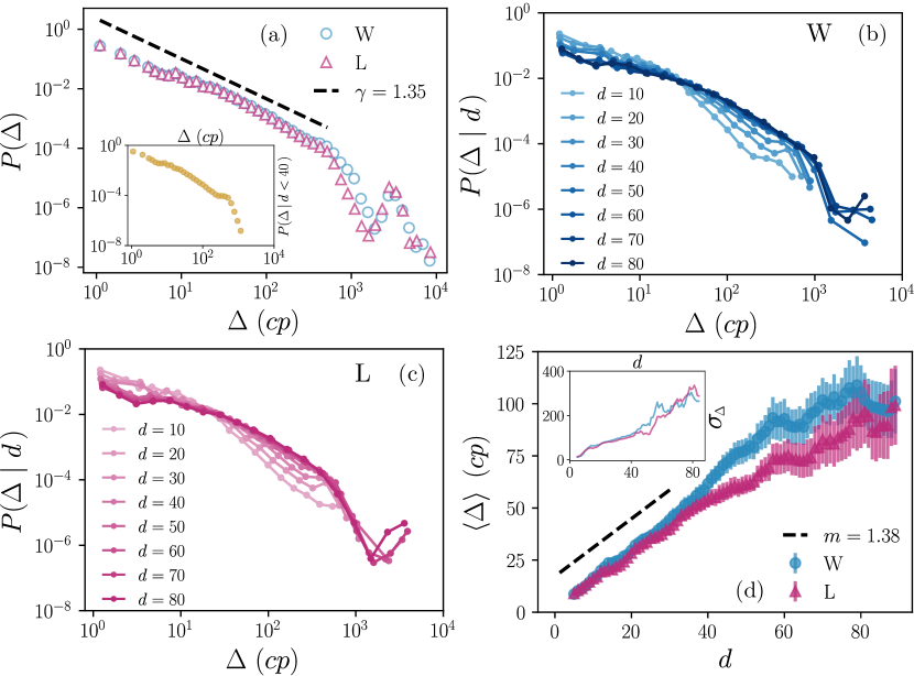
Figure 4: Complexity in the Decision-Making Process. (a) Distribution $P(\Delta)$ in groups of winning players (W) and losing players (L). Dashed lines show the theoretical distribution $P(\Delta)=C\Delta^{-\gamma}$. The inset shows the same probability distribution for $\Delta$ values observed at depths $d<40$. (b) and (c) show the distributions $P(\Delta|d)$ for different values of $d$ in W and L groups, respectively. (d) Mean value of $\Delta$ as a function of depth for W and L groups. The inset shows the standard deviation, $\sigma_{\Delta}$.

For this particular analysis, we used the FIDE dataset. First, we calculated the $\Delta$ vs. $d$ curves for all games and separated the dataset into two groups: in group W, we have the $\Delta$ values associated with the players who won the game, and in group L, those who lost. In this analysis, we excluded draws; we are interested in studying only decisive games. In Fig. 4 (a), we show the distribution $P(\Delta)$ for groups W and L. We can see a power-law trend over three orders of magnitude with a cutoff at $\Delta\approx 1000$. In that range, using the maximum likelihood method [37], we fit the curve associated with group W to the expression $P(\Delta)=C\Delta^{-\gamma}$, obtaining the value $\gamma=1.35$. The fact that the distribution is power-law-like shows that players can be subjected to a very heterogeneous landscape of decisions during the game. This is a clear indication of the emergence of complexity in the system. In the inset, we show the distribution for all the moves such $d<40$, $P(\Delta|d<40)$. For this plot, we took all $\Delta$ values from both groups. We can see that the small peak at $\Delta\approx 5000$ in the main figure disappears, indicating that these extreme values manifest only in the defining stage of the game.

This results show that $\Delta$ can take values that strongly depend on the stage of the game and, consequently, on the depth of the tree. To explore this further, we decided to study the distributions $P(\Delta|d)$ shown in Figs. 4 (b) and (c). For both groups, we can see that as $d$ increases the probability of finding high values of $\Delta$ increases, while the probability of finding low values decreases. It is interesting that, regardless of the depth, the distributions appear to have a heavy tail, indicating that the complexity in the decision-making process persists throughout all stages of the game.

To complement this analysis, in Fig. 4 (d), we present the evolution of the mean value $\left\langle\Delta\right\rangle$ as a function of depth $d$. The bars indicate the $99\%$ confidence interval around the estimator at a given depth. We observe an approximately linear evolution up to $d=40$. In this range, the mean value of $\Delta$ increases at a rate of $m=1.38$. As players delve deeper into the game, the game simplifies, and the analysis becomes more accurate. Consequently, more decisive positions emerge, and the $\Delta$ values increase. For $d>40$, we observe that the values of $\left\langle\Delta\right\rangle$ associated with group L begin to decrease. At this stage of the game, the matches start to be defined. Players who are losing begin to run out of tactical resources, and the decisions they make become less important, leading to the observed decrease in $\Delta$ values. The inset shows the evolution of the standard deviation estimator, $\sigma_{\Delta}$. We observe an increasing trend as players progress in the game. For $d>40$, we see something similar to what happens with the mean value, as the curve associated with losing players decreases slightly, indicating lower dispersion. It is interesting to note that this decrease in the standard deviation can be connected with a decrease in complexity levels compared to the winners’ group. In this sense, a loss of complexity in group L may be connected with a decrease in players’ performance.

III.4 Players’ Accuracy

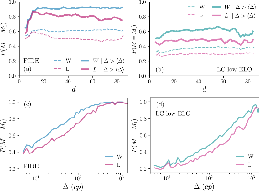
Figure 5: Players’ Accuracy. In (a) and (b), we show the probability that players execute the optimal move as a function of tree depth, $d$, for the FIDE and LC low ELO datasets, respectively. The datasets are separated into the W and L groups. Dashed lines show the total probability, and solid lines show the probability conditioned on the presence of tipping points. In (c) and (d), we show the probability that players execute the optimal move as a function of $\Delta$ value for the FIDE and LC low ELO datasets, respectively. The datasets are separated into the W and L groups.

In this section, we study the accuracy of the players. In Fig. 5 (a), we show the probability that players in the FIDE database execute the optimal move, $M=M_{1}$. The data is shown as a function of depth $d$ and separated into groups W and L. Dashed lines represent the total probability, $P(M=M_{1})$, and solid lines represent the probability conditioned on the presence of tipping points, $P(M=M_{1}~{}|~{}\Delta>\left\langle\Delta\right\rangle)$. Focusing on the latter, we observe that in both W and L, the probability shows an increasing trend up to $d\approx 10$. For $d>10$, in group W, the probability grows and stabilizes at approximately a constant value above $0.9$. On the other hand, in group L, we see that the probability shows a slightly decreasing trend across the entire range. A similar behavior is observed in the total probability, but with significantly lower values. In both cases, the probability associated with W is higher than that of L for all $d$. In Fig. 5 (b), we show the same relationships as in panel (a) but calculated on the LC low ELO dataset. In this case, the competitive level of the players is much lower, so the probability of executing the optimal move decreases significantly compared to elite players (FIDE). Nevertheless, as in the previous case, the probability associated with the winning group W is higher than that of L for all values of $d$.

It is important to note that regardless of the competitive level and the stage of the game, all players improve their performance in the presence of tipping point positions. This highlights a dependence of accuracy on the values of $\Delta$. To further investigate this, we study the probability the players make the best move $P(M=M_{1})$ vs. $\Delta$ in the FIDE and LC low ELO datasets. The results are shown in Fig. 5 (c) and (d). In both panels, we can see that the probability increases as $\Delta$ increases. However, FIDE players seem to increase at a faster rate. As expected, for the same value of $\Delta$, players in group W generally show a higher probability than those in group L in both datasets.

III.5 Null Model: Random Walk in the Chess Tree

In this section, we compare some of the results observed in the real system with a null model. The idea is to try to better understand the emergent properties associated with the parameter $\Delta$. Our null model is based on simulations of the chess game where competitors make random legal moves. To perform these simulations, we coded a Python script that simulates random games (RW) using the chess library as the core. With this script, we simulated 1000 games with a total depth of $D=80$ and then calculated the values of $\Delta$ for each of these games, following the same procedure as with the real games.

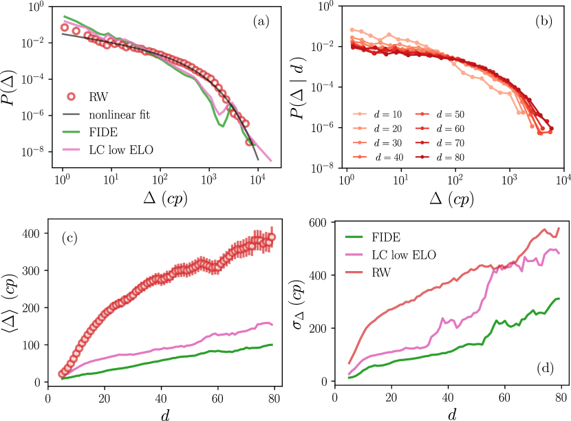
Figure 6: Results of the Null Model (RW). (a) Probability $P(\Delta)$ obtained from the null model (RW) compared with the FIDE and LC low ELO datasets. Solid line indicates the performed nonlinear fit to the distribution linked to RW data. (b) Depth-conditioned distributions. $P(\Delta|d)$ for the null model case. (c) Relationship $\left\langle\Delta\right\rangle$ vs. $d$ in the null model case, compared with the FIDE and LC low ELO datasets. The colors of the curves are referenced in panel (a). (d) Relationship $\sigma_{\Delta}$ vs. $d$ in the null model case, compared with the FIDE and LC low ELO datasets.

In Fig. 6(a), we compare the distribution $P(\Delta)$ obtained from the null model with the distributions obtained from the games in the FIDE and LC low ELO datasets. The distribution $P(\Delta)$ for the random case, can be fitted with a stretched exponential curve of the form,

$$f(x;\lambda,\beta)=\beta\lambda x^{\beta-1}e^{-\lambda x^{\beta}},$$

where $x=\Delta$, and $\beta$, $\lambda$ are free parameters. By performing the nonlinear fit, we obtain $\lambda=0.056$ and $\beta=0.584$, which gives us an excellent agreement, as we can see in the plot. On the other hand, we can see that in the simulated games, there are significantly higher values of $\Delta$ compared to the real cases. Moreover, the curve associated with lower-level players also shows the presence of higher values of $\Delta$ compared to elite players. These results uncover that the observed values of delta may depend on the competitive level of the players.

In Fig. 6 (b), we show the distributions of $P(\Delta|d)$ for the RW case. We can see that the distribution tends to flatten out as $d$ increases. Comparing this with what was obtained for the FIDE dataset in Fig. 4 (b) and (c), in RW, the curves are more similar to each other in the interval $100<\Delta<1000$, where for the FIDE case, significant differences are observed.

The values of $\Delta$ in the null model games are much larger at all depths than in the real case. This is clearly evidenced in the plot of $\left\langle\Delta\right\rangle$ vs. $d$ in Fig. 6 (c). In this case, we can see that the curve associated with RW takes values up to four times higher than the curve associated with FIDE. Likewise, the curve associated with lower-level players is significantly higher than that of elite players and much lower than for the null model. In Fig. 6(d), we show the evolution of the standard deviation estimator, $\sigma_{\Delta}$, as a function of depth. For all values of $d$, we see that the standard deviation increases as the competitive level decreases.

The results indicate that during the game, competitors tend to minimize the values of $\Delta$. This is consistent with what is observed in Fig. 5 (c) and (d), where we show that the accuracy of the players increase with $\Delta$. In other words, keeping low values of $\Delta$ can be seen as a strategy to maximize the probability of the opponent making a mistake.

Regarding the differences observed in groups of different levels, we can say that elite players, being better trained, can execute this strategy more effectively. That’s why the curves of $\left\langle\Delta\right\rangle$ and $\sigma_{\Delta}$ decrease compared to lower-level players. On the other hand, in random games, players make moves without any criteria, which is equivalent to the lowest competitive level, hence the curves increase.

III.6 Simple Model for Decision Making Process

The aim of this section is to integrate the empirical information gathered in our work and propose a toy model to simulate the decision-making process in the game. It is important to clarify that the model does not attempt to capture all the complexity inherent in the process, but rather to show that there are simple mechanisms that can explain the emergence of the global statistics we observe. The model is based on an agent that performs a walk in a complex tree. Starting from the root node and moving to the deepest level of the tree, the agent advances one node per time step. At each node of the tree, the agent has to decide which branch to continue with. This mechanism emulates players deciding which move to make. We propose that the number of branches in the tree follows a normal distribution, as is the case in the real tree (see Fig. 1 (b)). However, due to obvious computational limitations, we will use smaller trees than the real one, while maintaining approximately the relationship $\left\langle\mu\right\rangle/\sigma_{\mu}$ for greater structural similarity. Each node of the tree has attached a random value of $\Delta$. Upon reaching a node, the walkers use these values to decide which branch to continue based on the following algorithm:

1. The walker reaches a node at depth $d$ with $\mu$ outgoing branches.

2. It takes the values $\Delta_{i}$, $i=0,...,\mu$, from its neighbors at depth $d+1$,

   1. If $d<d^{*}$, it assigns the nodes a probability $p_{i}\propto\Delta_{i}^{-1}$, and uses this probability to decide which node to continue its walk on.

   2. If $d>d^{*}$, it chooses the neighbor with the smallest value of $\Delta$ and continues its walk through that node.

3. The procedure is repeated until reaching the deepest level of the tree, $d=D$.

The main idea of the algorithm is that the walkers move with preferential attachment towards nodes with smaller values of $\Delta$, thus emulating the minimization process observed in the empirical data. The value $d^{*}$ indicates a singular depth value in the tree. For $d<d^{*}$, we assume that the walker emulates a player who is not exactly sure which path to take, but their training allows them to identify some branches as better than others, so they move using the probabilities $p_{i}$. On the other hand, for $d>d^{*}$, we assume that as the walker delves deeper into the tree, their analytical power increases, and they know which is the optimal path to take. In this framework, we can relate $d^{*}$ to the competitive level. Given two walkers $i$ and $j$, if $d_{i}^{*}>d_{j}^{*}$, we say that walker $j$ is more skilled than $i$, because they can detect the optimal path at a smaller depth. To incorporate possible mistakes by the players into the model, we introduce noise into the system. We define $\eta$ as the probability of a walker choosing a path completely at random.

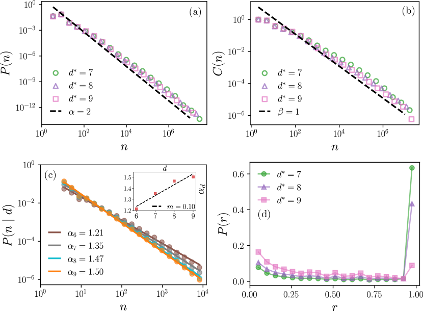
Figure 7: Model Results. (a) Node popularity distribution $P(n)$. Dashed lines show the theoretical distribution $P(n)=n^{-2}$. (b) Complementary cumulative distribution $C(n)$. Dashed lines show the theoretical distribution $C(n)=n^{-1}$. (c) Distributions $P(n|d)$ for the case $d^{*}=7$, at depths $d=6,7,8$, and $9$. Solid lines show the curves associated with a nonlinear fit of the distributions with the expression $P(n|d)=A~{}n^{-\alpha_{d}}$. The inset shows the relationship between the calculated $\alpha_{d}$ values and depth. (d) Ratio distribution $P(r)$.

In this framework, we simulate walks on trees with nodes having a branch distribution $\mu\sim N(6,2)$. To set the values of $\Delta$ in the tree, we use the non linear fit of the empirical probability distribution associated with the null model (see Fig. 6 (a)), as it provides information about the landscape of values that a walker might encounter. Using the inverse transform technique in the stretched exponential case, we then generated the sampling to set the value of $\Delta$ at each node. On the other hand, we set the noise level to a low value, $\eta=0.01$. To study the effect of the $d^{*}$ values, we conduct three simulations with $d^{*}=7$, $8$, and $9$. In each case, we simulate $50$ million walks. From the simulation results, we extracted the popularity of the nodes, and based on that, we calculated the distributions shown in Fig. 7. In panels (a) and (b), we show the distributions $P(n)$ and $C(n)$. We observe that the curves follow the trend $P(n)\propto n^{-2}$ and $C(n)\propto n^{-1}$, which is consistent with what is observed in distributions associated with real games. In Fig. 7 (c), we show the distributions $P(n|d)$ for $d=6,7,8,$ and $9$. These curves were calculated for the results associated with $d^{*}=7$. We observe distributions with a heavy tail, with the slope increasing slightly as the depth increases. Using the maximum likelihood method, we fit the distributions and obtained the exponents $\alpha_{d}$ for each case. In the inset of the panel, we show that the relationship $\alpha_{d}$ vs. $d$ follows a similar increasing trend as observed in the real data. In Fig. 7 (d), we show the distribution of ratios. We observe that around $r\approx 1$, $P(r)$ shows a peak that decreases as the value of $d^{*}$ increases. Additionally, we see that at $d\approx 0$, the probability value increases as the value of $r^{*}$ increases.

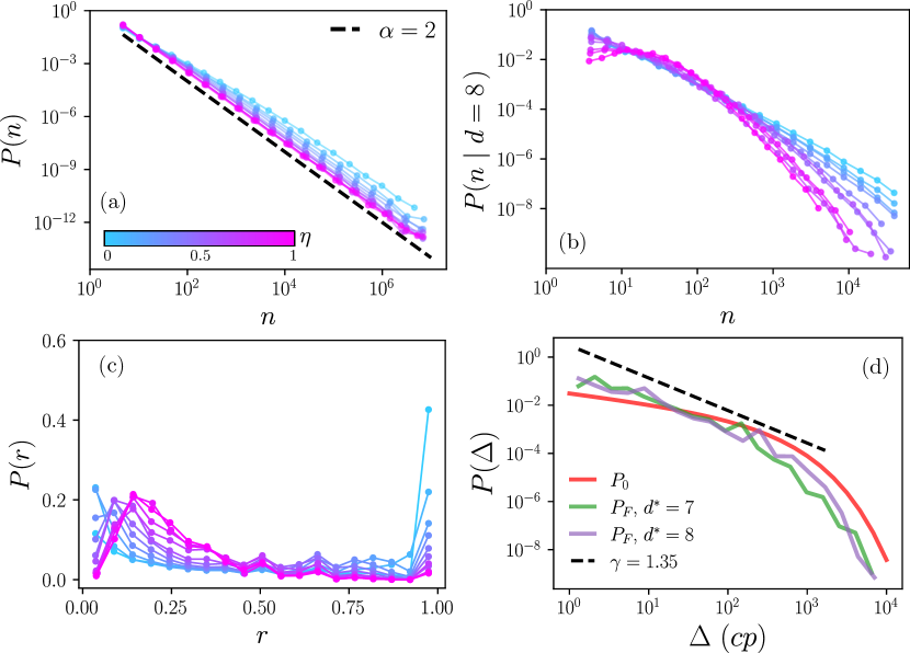
Figure 8: The curves in panels (a), (b) y (c) show the effect of the noise in the model for $d^{*}=8$. (a) Node popularity distribution $P(n)$, (b) Node popularity distribution at depth 8, $P(n|d=8)$, (c) Ratio distribution $P(r)$. The color bar relating the noise level to the curves is shown in panel (a). (d) Comparison between the initial probability distribution of $\Delta$ values, $P_{0}$, set at the beginning of the simulation, and the probability distribution of $\Delta$ values explored by the agents during the walk, $P_{F}$.

To test the effect of noise, we conducted a study varying the value of $\eta$. For these simulations, we fixed the parameter $d^{*}=8$. The tree structure and the number of walkers were kept the same as in the previous simulations. In Fig. 8 (a), (b), and (c), we show the distributions $P(n)$, $P(n|d=8)$, and $P(r)$, respectively. The curves represent the results for $\eta=0.0,0.1,...1.0$, where the cyan color in the graph indicates low noise levels, while magenta indicates high levels. Firstly, we observe that the noise level does not seem to significantly affect the exponent of the distribution $P(n)$ for large values of $n$. For high noise values, $\eta\to 1$, the curve closely resembles the theoretical one, $P(n)\propto n^{-2}$. Which is consistent with a random walk on an approximately regular tree. Secondly, we see that the distribution $P(n|d=8)$ becomes more homogeneous for high levels of noise, meaning that at the same level, we find similar popularity values. Lastly, in the distribution $P(r)$, we see that noise destroys the peak at $r\approx 1$ and creates another around $r\approx 1/6$. This is related to what is observed in $P(n|d=8)$: noise makes it equally likely to go to any node, and since the average number of exits from a node is $\left\langle\mu\right\rangle=6$, when it is equally likely to take any path, the value of $r$ around $1/6$ increases. Finally, in Fig. 8 (d), we compare the distribution of $\Delta$ values set as the initial condition, $P_{0}$, with the distribution of $\Delta$ values explored by the walkers during the simulations, $P_{F}$, for the cases $d^{*}=7,8$. As a reference, we show the theoretical curve $P(\Delta)\propto\Delta^{-\gamma}$ with $\gamma=1.35$, associated with the FIDE dataset, in dashed lines. We can see that the model approximately reproduces the process of minimizing $\Delta$ values observed empirically in Fig. 6 (a).

As we can see, our toy model roughly captures the general aspects of the global emergent properties of the system. This by no means implies that our model is capable of capturing the total complexity of decision-making dynamics; rather, it suggests that despite being an extremely complex system, the mechanisms generating the observed global emergent properties can be approximated by relatively simple mechanisms based on structural parameters of the tree and the process of minimizing $\Delta$.

IV Conclusions

The main goal of our work was to shed light on the microscopic mechanisms that generate global emergent properties of the system. In this framework, we decided to focus our analysis on the players’ decision-making process. To this end, we used the parameter $\Delta$ as a proxy, which indicates how crucial it is to make a good decision in a given position. We observed that as players progress through the game, they encounter positions with a wide range of $\Delta$ values, evidencing the complexity of the process. In this context, we noted statistically significant differences between groups of winners and losers, suggesting that a drop in the system’s complexity could be associated with a drop in players’ performance. This is somewhat similar to what is observed in so-called living systems, such as in nervous system diseases that affect neuron interactions [38], or with the death of mitochondria within cells [39]. When complexity decreases in these systems, their functioning is severely impacted. The loss of the delicate balance between inhibition and promotion, cooperation and competition in a complex system leads to the appearance of something abnormal. In the game of chess, we observed this effect manifesting in the drop of players’ competitive abilities.

On the other hand, by studying how well players choose the optimal move in a given position (accuracy), we found evidence that this improves in the presence of high $\Delta$ values. We also showed that this increase in accuracy is observed regardless of the players’ competitive level or whether they belong to winning or losing groups. To complement this analysis, we conducted a comparative study between the empirical data and the results of a null model based on players making random legal moves. We observed that players tend to decide guided by a process of minimizing $\Delta$ values, and that this process improves with the players’ competitive level. Note that this is consistent with our accuracy study. Given that players at any level become more accurate in the presence of positions with high $\Delta$ values, it is natural to think that, in the context of sporting competition, a winning strategy would be to make moves such that the opponent is left with positions having low $\Delta$ values. In this way the profit of the opponents is minimized and their probability of error is maximized.

Finally, using the set of empirical observations made in our work, we proposed a simple decision-making model. This model is based on agents walking in a complex tree where each node has a $\Delta$ value sampled from a power-law distribution. At each step, the agents have to decide which path to take, using a strategy that favors paths with nodes having small $\Delta$ values, attempting to emulate the minimization process observed in reality. We found that the simple mechanisms proposed in the model approximately generate the global emergent properties observed in the real system, demonstrating that the decision-making process, despite being extremely complex, can be explained using relatively simple evolution rules.

The framework, results, and analysis of the complexity of chess reported in this work can be useful for understanding several player’s behaviors, and also to improve the interaction of players with engines. Extensions of the statistic of critical points would have straightforward applications among the following lines that are currently under study. In the analysis of the behavior of players Chowdhary et al. [40] found that skilled players can be distinguished from the others based on their gaming behaviour where these differences appear from the very first moves of the game. Experts specialize and repeat the same openings while beginners explore and diversify more. Our results are in agreement with these findings and further specific analyses are possible to provide a better understanding of this topic. Another application of our work is in studying the popularity of opening lines. For instance, Lappo et al. [41] carried out an analysis of chess in the context of cultural evolution, describing multiple cultural factors that affect move choice. Also, our framework can be used to unveil risk patterns within chess games; complementing existing approaches to risk based on categorizing chess openings or entire games [42, 43]. The relationship between chess and Artificial Intelligence (AI) is synergetic. An analysis of AlphaZero systems suggests [15] that it may be possible to understand a neural network using human-defined chess concepts, even when it learns entirely on its own. More specifically, using a machine learning model Tijhuis et al. [44] showed that for predicting the level of a player the most important features to be considered during the match are both from theory, such as mobility at the end of the game and engine evaluation such as blunders and mistakes. Our analysis can provide new features to encode games and predict the level of expertise of players using AI.

References

- [1] Haroldo V Ribeiro, Satyam Mukherjee, and Xiao Han T Zeng. Anomalous diffusion and long-range correlations in the score evolution of the game of cricket. Physical Review E, 86(2):022102, 2012.
- [2] A Clauset, M Kogan, and S Redner. Safe leads and lead changes in competitive team sports. Physical Review E, 91(6):062815, 2015.
- [3] Dilan Patrick Kiley, Andrew J Reagan, Lewis Mitchell, Christopher M Danforth, and Peter Sheridan Dodds. Game story space of professional sports: Australian rules football. Physical Review E, 93(5):052314, 2016.
- [4] Sergio J Ibáñez, Aitor Mazo, Juarez Nascimento, and Javier García-Rubio. The relative age effect in under-18 basketball: Effects on performance according to playing position. PloS one, 13(7):e0200408, 2018.
- [5] Perrin E Ruth and Juan G Restrepo. Dodge and survive: Modeling the predatory nature of dodgeball. Physical Review E, 102(6):062302, 2020.
- [6] Johann H Martínez, David Garrido, José L Herrera-Diestra, Javier Busquets, Ricardo Sevilla-Escoboza, and Javier M Buldú. Spatial and temporal entropies in the spanish football league: A network science perspective. Entropy, 22(2):172, 2020.
- [7] Ken Yamamoto and Takuma Narizuka. Preferential model for the evolution of pass networks in ball sports. Physical Review E, 103(3):032302, 2021.
- [8] A Chacoma, Nahuel Almeira, Juan Ignacio Perotti, and Orlando Vito Billoni. Modeling ball possession dynamics in the game of football. Physical Review E, 102(4):042120, 2020.
- [9] A Chacoma, N Almeira, JI Perotti, and OV Billoni. Stochastic model for football’s collective dynamics. Physical Review E, 104(2):024110, 2021.
- [10] A Chacoma, OV Billoni, and MN Kuperman. Complexity emerges in measures of the marking dynamics in football games. Physical Review E, 106(4):044308, 2022.
- [11] Andrés Chacoma and Orlando V Billoni. Simple mechanism rules the dynamics of volleyball. Journal of Physics: Complexity, 3(3):035006, 2022.
- [12] Andrés Chacoma and Orlando V Billoni. Probabilistic model for padel games dynamics. Chaos, Solitons & Fractals, 174:113784, 2023.
- [13] Frédéric Prost. On the impact of information technologies on society: an historical perspective through the game of chess. In Andrei Voronkov, editor, Turing-100, volume 10 of EPiC Series, pages 268–277. EasyChair, 2012.
- [14] Claude E Shannon. Xxii. programming a computer for playing chess. The London, Edinburgh, and Dublin Philosophical Magazine and Journal of Science, 41(314):256–275, 1950.
- [15] Thomas McGrath, Andrei Kapishnikov, Nenad Tomašev, Adam Pearce, Martin Wattenberg, Demis Hassabis, Been Kim, Ulrich Paquet, and Vladimir Kramnik. Acquisition of chess knowledge in alphazero. Proceedings of the National Academy of Sciences, 119(47):e2206625119, 2022.
- [16] Xujun Duan, Wei Liao, Dongmei Liang, Lihua Qiu, Qing Gao, Chengyi Liu, Qiyong Gong, and Huafu Chen. Large-scale brain networks in board game experts: Insights from a domain-related task and task-free resting state. PLoS ONE, 7(3):1–11, 2012.
- [17] Mariano Sigman, Pablo Etchemendy, Diego Fernandez Slezak, and Guillermo A. Cecchi. Response time distributions in rapid chess: A large-scale decision making experiment. Frontiers in Neuroscience, 4:1, October 2010.
- [18] María Juliana Leone, Diego Fernandez Slezak, Diego Golombek, and Mariano Sigman. Time to decide: Diurnal variations on the speed and quality of human decisions. Cognition, 158:44 – 55, 2017.
- [19] Philippe Chassy and Fernand Gobet. Measuring chess experts’ single-use sequence knowledge: An archival study of departure from ’Theoretical’ openings. PLoS ONE, 6(11):e26692, November 2011.
- [20] Giovanni Sala and Fernand Gobet. Does chess instruction improve mathematical problem-solving ability? two experimental studies with an active control group. Learning & Behavior, pages 1–8, 2017.
- [21] Andrea Brancaccio and Fernand Gobet. Scientific explanations of the performance gender gap in chess and science, technology, engineering and mathematics (stem). Journal of Expertise/March, 6(1), 2023.
- [22] Bernd Blasius and Ralf Tönjes. Zipf’s Law in the Popularity Distribution of Chess Openings. Phys. Rev. Lett., 103:218701, Nov 2009.
- [23] Haroldo V. Ribeiro, Renio S. Mendes, Ervin K. Lenzi, Marcelo del Castillo-Mussot, and Luís A. N. Amaral. Move-by-move dynamics of the advantage in chess matches reveals population-level learning of the game. PLoS ONE, 8(1):e54165, 01 2013.
- [24] J. I. Perotti, H.H. Jo, A. L. Schaigorodsky, and O. V. Billoni. Innovation and nested preferential growth in chess playing behavior. EPL (Europhysics Letters), 104(4):48005, 2013.
- [25] Ana L. Schaigorodsky, Juan I. Perotti, and Orlando V. Billoni. Memory and long-range correlations in chess games. Physica A: Statistical Mechanics and its Applications, 394(0):304 – 311, 2014.
- [26] Arshia Atashpendar, Tanja Schilling, and Thomas Voigtmann. Sequencing chess. EPL (Europhysics Letters), 116(1):10009, 2016.
- [27] Ana L. Schaigorodsky, Juan I. Perotti, and Orlando V. Billoni. A study of memory effects in a chess database. PLOS ONE, 11(12):1–18, 12 2016.
- [28] Nahuel Almeira, Ana L Schaigorodsky, Juan I Perotti, and Orlando V Billoni. Structure constrained by metadata in networks of chess players. Scientific reports, 7(1):15186, 2017.
- [29] Giordano De Marzo and Vito DP Servedio. Quantifying the complexity and similarity of chess openings using online chess community data. Scientific Reports, 13(1):5327, 2023.
- [30] Marc Barthelemy. Statistical analysis of chess games: space control and tipping points. arXiv preprint arXiv:2304.11425, 2023.
- [31] Iossif Dorfman. The Method in Chess. 2001.
- [32] Mark E. Glickman. Chess rating systems. American Chess Journal, 3:59–102, 1995.
- [33] Lichess, website. https://lichess.org/.
- [34] The week in chess, website. https://theweekinchess.com/.
- [35] Lichess, database. https://database.lichess.org/.
- [36] Stockfish engine. https://stockfishchess.org/.
- [37] Aaron Clauset, Cosma Rohilla Shalizi, and Mark EJ Newman. Power-law distributions in empirical data. SIAM review, 51(4):661–703, 2009.
- [38] Ezequiel V Albano. Self-organized collective displacements of self-driven individuals. Physical Review Letters, 77(10):2129, 1996.
- [39] Nahuel Zamponi, Emiliano Zamponi, Sergio A Cannas, Orlando V Billoni, Pablo R Helguera, and Dante R Chialvo. Mitochondrial network complexity emerges from fission/fusion dynamics. Scientific reports, 8(1):1–10, 2018.
- [40] Sandeep Chowdhary, Iacopo Iacopini, and Federico Battiston. Quantifying human performance in chess. Scientific Reports, 13(1):2113, 2023.
- [41] Egor Lappo, Noah A Rosenberg, and Marcus W Feldman. Cultural transmission of move choice in chess. Proceedings of the Royal Society B, 290(2011):20231634, 2023.
- [42] Johannes Carow and Niklas M Witzig. Time pressure and strategic risk-taking in professional chess. Technical report, 2024.
- [43] Anna Dreber, Christer Gerdes, and Patrik Gränsmark. Beauty queens and battling knights: Risk taking and attractiveness in chess. Journal of Economic Behavior & Organization, 90:1–18, 2013.
- [44] Tim Tijhuis, Paris Mavromoustakos Blom, and Pieter Spronck. Predicting chess player rating based on a single game. In 2023 IEEE Conference on Games (CoG), pages 1–8. IEEE, 2023.