Large-Scale Contextual Market Equilibrium Computation through Deep Learning

Abstract

Market equilibrium is one of the most fundamental solution concepts in economics and social optimization analysis. Existing works on market equilibrium computation primarily focus on settings with a relatively small number of buyers. Motivated by this, our paper investigates the computation of market equilibrium in scenarios with a large-scale buyer population, where buyers and goods are represented by their contexts. Building on this realistic and generalized contextual market model, we introduce MarketFCNet, a deep learning-based method for approximating market equilibrium. We start by parameterizing the allocation of each good to each buyer using a neural network, which depends solely on the context of the buyer and the good. Next, we propose an efficient method to estimate the loss function of the training algorithm unbiasedly, enabling us to optimize the network parameters through gradient descent. To evaluate the approximated solution, we introduce a metric called Nash Gap, which quantifies the deviation of the given allocation and price pair from the market equilibrium. Experimental results indicate that MarketFCNet delivers competitive performance and significantly lower running times compared to existing methods as the market scale expands, demonstrating the potential of deep learning-based methods to accelerate the approximation of large-scale contextual market equilibrium.

1 Introduction

Market equilibrium is a solution concept in microeconomics theory, which studies how individuals amongst groups will exchange their goods to get each one better off [51]. The importance of market equilibrium is evidenced by the 1972 Nobel Prize awarded to John R. Hicks and Kenneth J. Arrow “for their pioneering contributions to general economic equilibrium theory and welfare theory” [58]. Market equilibrium has wide application in fair allocation [32], as a few examples, fairly assigning course seats to students [11] or dividing estates, rent, fares, and others [35]. Besides, market equilibrium are also considered for ad auctions with budget constraints where money has real value [15, 16].

Existing works often use traditional optimization method or online learning technique to solve market equilibrium, which can tackle one market with around $400$ buyers and goods in experiments [30, 52]. However, in realistic scenarios, there might be millions of buyers in one market (e.g. job market, online shopping market). In these scenarios, the description complexity for the market is $O(nm)$ and it needs at least $O(nm)$ cost to do one optimization step for the market, if there are $n$ buyers and $m$ goods in the market, which is unacceptable when $n$ is extremely large and potentially infinite. In this case, and traditional optimization methods do not work anymore.

However, contextual models come to the rescue. The success of contextual auctions[21, 5] demonstrate the power of contextual models, in which each bidder and item are represented as context and the value (or the distribution) of item to bidder is determined by the contexts. In this way, auctions as well as other economic problems can be described in a more memory-efficient way, making it possible to accelerate the computation on these problems. Inspired by the models of contextual auctions, we propose the concept of contextual markets in a similar way. We verify that contextual markets can be useful to model large-scale markets aforementioned, since the real market can be assumed to be within some low dimension space, and the values of goods to buyers are often not hard to speculate given the knowledge of goods and buyers [46, 45]. Besides, contextual models never lose expressive power compared with raw models[7], giving contextual markets capabilities to generalize over traditional markets.

This paper initiates the study of deep learning for contextual market equilibrium computation with a large number of buyers. The description complexity of contextual markets is $O(n+m)$, if there are $n$ buyers and $m$ items in the market, making them memory-efficient and helpful for follow-up equilibrium computation while holding the market structure. Following the framework of differentiable economics [18, 26, 62], we propose a deep-learning based approach, MarketFCNet, in which one optimization step costs only $O(m)$ rather than $O(nm)$ in traditional methods, greatly accelerating the computation of market equilibrium. MarketFCNet takes the representations of one buyer and one good as input, and outputs the allocation of the good to the buyer. The training on MarketFCNet targets at an unbiased estimator of the objective function of EG-convex program, which can be formed by independent samples of buyers. By this way, we optimize the allocation function on “buyer space” implicitly, rather than optimizing the allocation to each buyer directly. Therefore, MarketFCNet can reduce the algorithm complexity such that it becomes independent of $n$, i.e., the number of buyers.

The effectiveness of MarketFCNet is demonstrated by our experimental results. As the market scale expands, MarketFCNet delivers competitive performance and significantly lower running times compared to existing methods in different experimental settings, demonstrating the potential of deep learning-based methods to accelerate the approximation of large-scale contextual market equilibrium.

The contributions of this paper consist of three parts,

• We proposes a method, MarketFCNet, to approximate the contextual market equilibrium in which the number of buyers is large.

• We proposes Nash Gap to quantify the deviation of the given allocation and price pair from the market equilibrium.

• We conduct extensive experiments, demonstrating promising performance on the approximation measure and running time compared with existing methods.

2 Related Works

The history of market equilibrium arises from microeconomics theory, where the concept of competitive equilibrium [51, §10] was proposed, and the existence of market equilibrium is guaranteed in a general setting [3, 61]. Eisenberg and Gale [28] first considered the linear market case, and proved that the solution of EG-convex program constitutes a market equilibrium, which lays the polynomial-time algorithmic foundations for market equilibrium computation. Eisenberg [27] later showed that EG program also works for a class of CCNH utility functions. Shmyrev program later is also proposed to solve market equilibrium with linear utility with a perspective shift from allocation to price [57], while Cole et al. [14] later found that Shmyrev program is the dual problem of EG program with a change of variables. There are also a branch of literature that consider computational perspective in more general settings such as indivisible goods [54, 19, 20] and piece-wise linear utility [60, 33, 34].

There are abundant of works that present algorithms to solve the market equilibrium and shows the convergence results theoretically [13]. Gao and Kroer [30] discusses the convergence rates of first-order algorithms for EG convex program under linear, quasi-linear and Leontief utilities. Nan et al. [52] later designs stochastic optimization algorithms for EG convex program and Shmyrev program with convergence guarantee and show some economic insight. Jalota et al. [42] proposes an ADMM algorithm for CCNH utilities and shows linear convergence results. Besides, researchers are more engaged in designing dynamics that possess more economic insight. For example, PACE dynamic [32, 48, 65] and proportional response dynamic [63, 66, 12], though the original idea of PACE arise from auction design [16, 15].

With the fast growth of machine learning and neural network, many existing works aim at resolving economic problem by deep learning approach, which falls into the differentiate economy framework [26]. A mainstream is to approximate the optimal auction with differentiable models by neural networks [25, 29, 36, 55]. The problem of Nash equilibrium computation in normal form games [22, 50, 23] and optimal contract design [62] through deep learning also attracts researchers’ attentions. Among these methodologies, transformer architecture [50, 21, 47] is widely used in solving economic problems.

To the best of our knowledge, no existing works try to approximate market equilibrium through deep learning. Besides, although some literature focuses on low-rank markets and representative markets [46, 45], our works firstly propose the concept of contextual market. We believe that our approach will pioneer a promising direction for large-scale contextual market equilibrium computation.

3 Contextual Market Modelling

In this section, we focus on the model of contextual market equilibrium in which goods are assumed to be divisible. Let the market consist of $n$ buyers, denoted as $1,...,n$, and $m$ goods, denoted as $1,...,m$. We denote $[k]$ as the abbreviation of the set $\{1,2,\dots,k\}$. Each buyer ${i\in[n]}$ has a representation $b_{i}$, and each good ${j\in[m]}$ has a representation $g_{j}$. We assume that $b_{i}$ belongs to the buyer representation space $\mathcal{B}$, and $g_{j}$ belongs to the good representation space $\mathcal{G}$. For a buyer with representation $b\in\mathcal{B}$, she has budget $B(b)>0$. Denote $Y(g)>0$ as the supply of good with representation $g$. Although many existing works [30] assume that each good $j$ has unit supply (i.e. $Y(g)\equiv 1$ for all $g\in\mathcal{G}$) without loss of generality, their results can be easily generalized to our settings.

An allocation is a matrix ${\bm{x}}=(x_{ij})_{{i\in[n]},{j\in[m]}}\in\mathbb{R}^{n\times m}_{+}$, where $x_{ij}$ is the amount of good $j$ allocated to buyer $i$. We denote ${\bm{x}}_{i}=(x_{i1},\dots,x_{im})$ as the vector of bundle of goods that is allocated to buyer $i$. The buyers’ utility function is denoted as $u:\mathcal{B}\times\mathbb{R}^{m}_{+}\to\mathbb{R}_{+}$, here $u(b_{i};{\bm{x}}_{i})$ denotes the utility of buyer $i$ with representation $b_{i}$ when she chooses to buy ${\bm{x}}_{i}$. We denote $u_{i}({\bm{x}}_{i})$ as an equivalent form of $u(b_{i};{\bm{x}}_{i})$ and often refer them as the same thing. Similarly, $B(b_{i}),Y(g_{j})$ and $B_{i},Y_{j}$ are often referred to as the same thing, respectively.

Let ${\bm{p}}=(p_{1},\dots,p_{m})\in\mathbb{R}^{m}_{+}$ be the prices of the goods, the demand set of buyer with representation $b_{i}$ is defined as the set of utility-maximizing allocations within budget constraint.

$$D(b_{i};{\bm{p}})\coloneqq\operatorname*{arg\,max}_{{\bm{x}}_{i}}\left\{u(b_{i};{\bm{x}}_{i})\mid{\bm{x}}_{i}\in\mathbb{R}^{m}_{+},\,\langle{\bm{p}},{\bm{x}}_{i}\rangle\leq B(b_{i})\right\}.$$ (1)

A contextual market is a 4-tuple: $\mathcal{M}=\langle n,m,(b_{i})_{i\in[n]},(g_{j})_{j\in[m]}\rangle$, where buyer utility $u(b_{i};{\bm{x}}_{i})$ is known given the information of the market. We also assume budget function $B:\mathcal{B}\to\mathbb{R}_{+}$ represents the budget of buyers and capacity function $Y:\mathcal{G}\to\mathbb{R}_{+}$ represents the supply of goods. All of $u$, $B$ and $Y$ are assumed to be public knowledge and excluded from a market representation. This assumption mainly comes from two aspects: (1) these functions can be learned from historical data and (2) budgets and supplies can be either encoded in $b$ and $g$ in some way.

The market equilibrium is represented as a pair $({\bm{x}},{\bm{p}})$, ${\bm{x}}\in\mathbb{R}_{+}^{n\times m},\ {\bm{p}}\in\mathbb{R}_{+}^{m}$, which satisfies the following conditions.

• Buyer optimality: ${\bm{x}}_{i}\in D(b_{i},{\bm{p}})$ for all ${i\in[n]}$,

• Market clearance: $\sum_{i=1}^{n}x_{ij}\leq Y(g_{j})$ for all ${j\in[m]}$, and equality must hold if $p_{j}>0$.

We say that $u_{i}$ is homogeneous (with degree $1$) if it satisfies $u_{i}(\alpha{\bm{x}}_{i})=\alpha u_{i}({\bm{x}}_{i})$ for any ${\bm{x}}_{i}\geq 0$ and $\alpha>0$ [53, §6.2]. Following existing works, we assume that $u_{i}$s are CCNH utilities, where CCNH represents for concave, continuous, non-negative, and homogeneous functions[30]. For CCNH utilities, a market equilibrium can be computed using the following Eisenberg-Gale convex program (EG):

$$\max\sum_{i=1}^{n}B_{i}\log u_{i}({\bm{x}}_{i})\quad{\rm s.t.}\ \sum_{i=1}^{n}x_{ij}\leq Y_{j},\ {\bm{x}}\geq 0.$$ (EG)

Theorem 3.1 shows that the market equilibrium can be represented as the optimal solution of (EG).

Theorem 3.1 (Gao and Kroer [30]).

Let $u_{i}$ be concave, continuous, non-negative and homogeneous (CCNH). Assume $u_{i}(\mathbf{1})>0$ for all $i$. Then, (i) (EG) has an optimal solution and (ii) any optimal solution ${\bm{x}}$ to (EG) together with its optimal Lagrangian multipliers ${\bm{p}}^{*}\in\mathbb{R}_{+}^{m}$ constitute a market equilibrium, up to arbitrary assignment of zero-price items. Furthermore, $\langle{\bm{p}}^{*},{\bm{x}}^{*}_{i}\rangle=B_{i}$ for all $i$.

Based on Theorem 3.1, it’s easy to find that we can always assume $\sum_{i\in[n]}x_{ij}=Y_{j}$ while preserving the existence of market equilibrium, which states as follows.

Proposition 3.2.

Following the assumptions in Theorem 3.1. For the following EG convex program with equality constraints,

$$\max\sum_{i=1}^{n}B_{i}\log u_{i}({\bm{x}}_{i})\quad{\rm s.t.}\ \sum_{i=1}^{n}x_{ij}=Y_{j},\ {\bm{x}}\geq 0.$$ (2)

Then, an optimal solution ${\bm{x}}^{*}$ together with its Lagrangian multipliers ${\bm{p}}^{*}\in\mathbb{R}^{m}_{+}$ constitute a market equilibrium. Moreover, assume more that for each good $j$, there is some buyer $i$ such that $\frac{\partial u_{i}}{\partial x_{ij}}>0$ always hold whenever $u_{i}({\bm{x}}_{i})>0$, then all prices are strictly positive in market equilibrium. As a consequence, Equation EG and Equation 2 derive the same solution.

We leave all proofs to Appendix B. Since the additional assumption in Proposition 3.2 is fairly weak, without further clarification, we always assume the conditions in Proposition 3.2 hold and the market clearance condition becomes $\sum_{i\in[n]}x_{ij}=Y(g_{j}),\ \forall{j\in[m]}$.

4 MarketFCNet

In this section, we introduce the MarketFCNet (denoted as Market Fully-Connected Network) approach to solve the market equilibrium when the number of buyers is large and potentially infinite. MarketFCNet is a sampling-based methodology, and the key point is to design an unbiased estimator of an objective function whose solution coincides with the market equilibrium. The main advantage is that it has the potential to fit the infinite-buyer case without scaling the computational complexity. Therefore, MarketFCNet is scalable with the number of buyers varies.

4.1 Problem Reformulation

Following the idea of differentiable economics [26], we consider parameterized models to represent the allocation of good $j$ to buyer $i$, denoted as $x_{\theta}(b_{i},g_{j})$, and call it allocation network, where $\theta$ is the network parameter. Given buyer $i$ and good $j$, the network can automatically compute the allocation $x_{ij}=x_{\theta}(b_{i},g_{j})$. The allocation to buyer $i$ is represented as ${\bm{x}}_{i}={\bm{x}}_{\theta}(b_{i},{\bm{g}})$ and the allocation matrix is represented as ${\bm{x}}={\bm{x}}_{\theta}({\bm{b}},{\bm{g}})$. Then the market clearance constraint can be reformulated as $\sum_{i\in[n]}x_{\theta}(b_{i},g_{j})=Y(g_{j}),\forall{j\in[m]}$ and the price constraint can be reformulated as ${\bm{x}}_{\theta}({\bm{b}},{\bm{g}})\geq 0$. Let $b$ be uniformly distributed from $\mathcal{B}=\{b_{i}:{i\in[n]}\}$, then the EG program (EG) becomes,

$$\max_{x_{\theta}} \quad\mathrm{OBJ}(x_{\theta})=\mathbb{E}_{b}[B(b)\log u(b;{\bm{x}}_{\theta}(b,{\bm{g}}))]$$ (EG-FC)

$$\mathrm{s.t.} \quad\mathbb{E}_{b}[x_{\theta}(b,g_{j})]=Y(g_{j})/n,\forall{j\in[m]}$$

$$\quad{\bm{x}}_{\theta}({\bm{b}},{\bm{g}})\geq 0$$

For simplicity, we take $Y(g_{j})/n\equiv 1$ for all $g_{j}$.

4.2 Optimization

The second constraint in (EG-FC) can be easily handled by the network architecture (for example, network with a softplus layer $\sigma(x)=\log(1+\exp(x)$). As for the first constraint, from Theorem 3.1, we know the prices of goods are simply the Lagrangian multipliers for the first constraint in (EG-FC). Therefore, we employ the Augmented Lagrange Multiplier Method (ALMM) to solve the problem (EG-FC). We define $\mathcal{L}_{\rho}(x_{\theta},\lambda)$ as the Lagrangian, which has the form:

$$\mathcal{L}_{\rho}(x_{\theta};\bm{\lambda})= -\mathrm{OBJ}(x_{\theta})+\sum_{j=1}^{m}\lambda_{j}\left(\mathbb{E}_{b}[x_{\theta}(b,g_{j})]-1\right)+\frac{\rho}{2}\sum_{j=1}^{m}\left(\mathbb{E}_{b}[x_{\theta}(b,g_{j})]-1\right)^{2}$$ (3)

Directly computing the objective function seems intractable due to the potentially infinite data size. Therefore, we follow the framework in learning theory culture that we only guarantee to achieve an unbiased gradient of the objective function [1, 8]. The training process of MarketFCNet is presented in Figure 1.

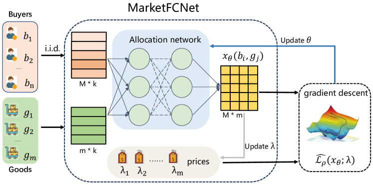
Figure 1: Training process of MarketFCNet. On each iteration, the batch of $M$ independent buyers are drawn. each buyer and each good are represented as $k$-dimension context. The $(i,j)$’th element in the allocation matrix represents the allocation computed from $i$’th buyer and $j$’th good. MarketFCNet training process alternates between the training of allocation network and prices. The training of allocation network need to achieve an unbiased estimator $\widehat{\mathcal{L}}_{\rho}(x_{\theta};\lambda)$ of the loss function $\mathcal{L}_{\rho}(x_{\theta};\lambda)$, followed by gradient descent. The training of prices need to get an unbiased estimator $\widehat{\Delta}\lambda_{j}$ of $\Delta\lambda_{j}$, followed by ALMM updating rule $\lambda_{j}\leftarrow\lambda_{j}+\beta_{t}\widehat{\Delta}\lambda_{j}$.

To finish the ALMM algorithm, we need to obtain unbiased estimators of following two expressions.

• An unbiased estimator of $\mathcal{L}_{\rho}(x_{\theta};\bm{\lambda})$.

• An unbiased estimator of $\Delta\lambda_{j}$, where $\Delta\lambda_{j}$ is given by $\textstyle\Delta\lambda_{j}=\rho\left(\mathbb{E}_{b}[x_{\theta}(b,g_{j})]-1\right)$.

Unbiased estimator of $\Delta\lambda_{j}$

We aim to obtain an unbiased estimator of $\mathbb{E}_{b}[x_{\theta}(b,g_{j})]$. By applying Monte Carlo method, we can choose batch size $M$ and sample $b_{1},b_{2},...,b_{M}\sim U(\mathcal{B})$, then $\frac{1}{M}\sum_{i=1}^{M}x_{\theta}(b_{i},g_{j})$ forms an unbiased estimator.

Unbiased estimator of $\mathcal{L}_{p}(x_{\theta};\bm{\lambda})$

For $\mathrm{OBJ}(x_{\theta})$ and the second term, the technique to achieve an unbiased estimator is similar. $u(b;x_{\theta}(b,{\bm{g}}))$ in $\mathrm{OBJ}(x_{\theta})$ can be calculated directly by summing over all goods. For the last term, notice that

$$\left(\mathbb{E}_{b}\left[x_{\theta}(b,g_{j})\right]-1\right)^{2}=\left(\mathbb{E}_{b}\left[x_{\theta}(b,g_{j})\right]-1\right)\cdot\left(\mathbb{E}_{b^{\prime}}\left[x_{\theta}(b^{\prime},g_{j})\right]-1\right)$$ (4)

Therefore, we can sample $b_{1},...,b_{M},b^{\prime}_{1},...,b^{\prime}_{M}\sim U(\mathcal{B})$ and compute

$$\frac{\rho}{2}\cdot\frac{1}{M}\sum_{i=1}^{M}\sum_{j=1}^{m}\left(x_{\theta}(b_{i},g_{j})-1\right)\cdot\left(x_{\theta}(b^{\prime}_{i},g_{j})-1\right)$$ (5)

which provides an unbiased estimator for the last term, capturing the squared deviation of output allocations from the constraint.

5 Performance Measures of Market Equilibrium

In this section, we propose Nash Gap to measure the performance of an approximated market equilibrium and show that Nash Gap preserves the economic interpretation for market equilibrium. To introduce Nash Gap, we first introduce two types of welfare, Log Nash Welfare and Log Fixed-price Welfare in Definition 5.1 and Definition 5.2, respectively.

Definition 5.1 (Log Nash Welfare).

The Log Nash Welfare (abbreviated as $\mathrm{LNW}$) is defined as

$$\mathrm{LNW}({\bm{x}})=\frac{1}{B_{\mathrm{total}}}\sum_{i\in[n]}B_{i}\log u_{i}({\bm{x}}_{i}),$$ (6)

where $B_{\mathrm{total}}=\sum_{i\in[n]}B_{i}$ is the total budgets for buyers.

Notice that $\mathrm{LNW}({\bm{x}})$ is identical to the objective function in Equation EG, differing only in the constant term coefficient.

Definition 5.2 (Fixed-price and Log Fixed-price Welfare).

We define the fixed-price utility for buyer $i$ as,

$$\tilde{u}(b_{i};{\bm{p}})=\max_{{\bm{x}}_{i}}\{u(b_{i};{\bm{x}}_{i})\mid{\bm{x}}_{i}\in\mathbb{R}^{m}_{+},\langle{\bm{p}},{\bm{x}}_{i}\rangle\leq B(b_{i})\}$$ (7)

which represents the optimal utility that buyer $i$ can obtain at the price level ${\bm{p}}$, regardless of the market clearance constraints. The Log Fixed-price Welfare (abbreviated as $\mathrm{LFW}$) is defined as the logarithm of Fixed-price Welfare,

$$\mathrm{LFW}({\bm{p}})=\frac{1}{B_{\mathrm{total}}}\sum_{i\in[n]}B_{i}\log\tilde{u}_{i}({\bm{p}})$$ (8)

Based on these definitions, we present the definition of Nash Gap.

Definition 5.3 (Nash Gap).

We define Nash Gap (abbreviated as NG) as the difference of Log Nash Welfare and Log Fixed-price Welfare, i.e.

$$\mathrm{NG}({\bm{x}},{\bm{p}})=\mathrm{LFW}({\bm{p}})-\mathrm{LNW}({\bm{x}})$$ (9)

5.1 Properties of Nash Gap

To show why $\mathrm{NG}$ is useful in the measure of market equilibrium, we first observe that,

Proposition 5.4 (Price constraints).

If $({\bm{x}},{\bm{p}})$ constitute a market equilibrium, the following identity always hold,

$$\sum_{j\in[m]}p_{j}Y_{j}=\sum_{i\in[n]}B_{i}$$ (10)

Below, we state the most important theorem in this paper.

Theorem 5.5.

Let $({\bm{x}},{\bm{p}})$ be a pair of allocation and price. Assuming the allocation satisfies market clearance and the price meets price constraint, then we have $\mathrm{NG}({\bm{x}},{\bm{p}})\geq 0$.

Moreover, $\mathrm{NG}({\bm{x}},{\bm{p}})=0$ if and only if $({\bm{x}},{\bm{p}})$ is a market equilibrium.

Theorem 5.5 show that Nash Gap is an ideal measure of the solution concept of market equilibrium, since it holds following properties,

• $\mathrm{NG}({\bm{x}},{\bm{p}})$ is continuous on the inputs $({\bm{x}},{\bm{p}})$.

• $\mathrm{NG}({\bm{x}},{\bm{p}})\geq 0$ always hold. (under conditions in Theorem 5.5)

• $\mathrm{NG}({\bm{x}},{\bm{p}})=0$ if and only if $({\bm{x}},{\bm{p}})$ meets the solution concept.

• The computation of $\mathrm{NG}$ does not require the knowledge of an equilibrium point $({\bm{x}}^{*},{\bm{p}}^{*})$

Since some may argue that $\mathrm{NG}({\bm{x}},{\bm{p}})$ is not intuitive to understand, we consider some more intuitive measures, the Euclidean distance to the market equilibrium, i.e., $||{\bm{x}}-{\bm{x}}^{*}||$ and $||{\bm{p}}-{\bm{p}}^{*}||$, as well as the difference on Weighted Social Welfare, $|\mathrm{WSW}({\bm{x}})-\mathrm{WSW}({\bm{x}}^{*})|$, where $\mathrm{WSW}({\bm{x}})\coloneqq\sum_{i\in[n]}\frac{B_{i}}{B_{\mathrm{total}}}u_{i}({\bm{x}}_{i})$, and show the connection between $\mathrm{NG}$ and these intuitive measures.

Proposition 5.6.

Under some technical assumptions (which is presented in Section B.4), if $\mathrm{NG}({\bm{x}},{\bm{p}})=\varepsilon$, we have:

• $||{\bm{p}}-{\bm{p}}^{*}||=O(\sqrt{\varepsilon})$.

• $||{\bm{x}}_{i}-{\bm{x}}_{i}^{*}||=O(\sqrt{\varepsilon})$ for all $i$.

• $|\mathrm{WSW}({\bm{x}})-\mathrm{WSW}({\bm{x}}^{*})|=O(\varepsilon)$.

Finally, we give a saddle-point explaination for Nash Gap.

Corollary 5.7.

Within market clearance and price constraint, we have

$$\min_{\bm{p}}\mathrm{LFW}({\bm{p}})=\max_{\bm{x}}\mathrm{LNW}({\bm{x}})$$ (11)

Corollary 5.7 provides an economic interpretation for GAP. Market equilibrium can be seen as the saddle point over social welfare, and the social welfare for ${\bm{x}}$ can be actually implemented while the social welfare for ${\bm{p}}$ is virtual and desired by buyers. Nash Gap measures the gap between the “desired welfare” and the “implemented welfare” for buyers.

5.2 Measures in General Cases

Since $\mathrm{NG}$ only works for $({\bm{x}},{\bm{p}})$ that satisfies market clearance and price constraints, we generalize the measure of $\mathrm{NG}$ to a more general case, which need to give a measure for all positive $({\bm{x}},{\bm{p}})$.

We first notice that any equilibrium must satisfy the conditions of market clearance and price constraint, we first make a projection on arbitrary positive $({\bm{x}},{\bm{p}})$ to the space where these constraints hold. Specifically, if we let

$$\alpha_{j}= \frac{V_{j}}{\sum_{i}x_{ij}},\quad\tilde{x}_{ij}=x_{ij}\cdot\alpha_{j}\qquad \beta=\frac{\sum_{i}B_{i}}{\sum_{j}V_{j}p_{j}},\quad\tilde{p}_{j}=\beta\cdot p_{j}$$ (12)

then $(\tilde{{\bm{x}}},\tilde{{\bm{p}}})$ satisfies these constraints and we consider $\mathrm{NG}(\tilde{{\bm{x}}},\tilde{{\bm{p}}})$ as the equilibrium measure.

Besides, we also need to measure how far is the point $({\bm{x}},{\bm{p}})$ to the space within the conditions of market clearance and price constraint. we propose following two measurement, called Violation of Allocation (abbreviated as $\mathrm{VoA}$) and Violation of Price (abbreviated as $\mathrm{VoP}$), respectively.

$$\mathrm{VoA}({\bm{x}})\coloneqq \frac{1}{m}\sum_{j}|\log\alpha_{j}|,\qquad\mathrm{VoP}({\bm{p}})\coloneqq|\log\beta|$$ (13)

From the expressions of $\mathrm{VoA}$ and $\mathrm{VoP}$, we know that these two constraints hold if and only if $\mathrm{VoA}({\bm{x}})=0$ and $\mathrm{VoP}({\bm{p}})=0$.

We argue that this projection is of economic meaning. If $({\bm{x}},{\bm{p}})$ constitute a market equilibrium and we scale budget with a factor of $\beta$, then $({\bm{x}},\beta{\bm{p}})$ constitute a market equilibrium in the new market. Similarly, if we scale the value for each buyer with factor $1/\bm{\alpha}$ (here $\bm{\alpha}$ can be a vector in $\mathbb{R}^{m}_{+}$) and capacity with factor $\alpha$, then, $(\bm{\alpha}{\bm{x}},\frac{1}{\bm{\alpha}}{\bm{p}})$ constitute a market equilibrium in the new market. These instances are evidence that market equilibrium holds a linear structure over market parameters. Therefore, a linear projection can eliminate the effect from linear scaling, while preserving the effect from orthogonal errors.

Notice that ${\bm{x}}=\tilde{{\bm{x}}}$ and ${\bm{p}}=\tilde{{\bm{p}}}$ if and only if $\mathrm{VoA}({\bm{x}})=0$ and $\mathrm{VoP}({\bm{p}})=0$, respectively. From Theorem 5.5 We can easy derive following statements:

Proposition 5.8.

For arbitrary ${\bm{x}}\in\mathbb{R}^{n\times m}_{+},{\bm{p}}\in\mathbb{R}^{m}_{+}$, we have $\mathrm{VoA}({\bm{x}})\geq 0,\mathrm{VoP}({\bm{p}})\geq 0,\mathrm{NG}(\tilde{{\bm{x}}},\tilde{{\bm{p}}})\geq 0$ always hold. Moreover, $({\bm{x}},{\bm{p}})$ is a market equilibrium if and only if $\mathrm{VoA}({\bm{x}})=\mathrm{VoP}({\bm{p}})=\mathrm{NG}(\tilde{{\bm{x}}},\tilde{{\bm{p}}})=0$.

Proposition 5.8 is a certificate that $\mathrm{VoA}({\bm{x}}),\mathrm{VoP}({\bm{p}}),\mathrm{NG}(\tilde{{\bm{x}}},\tilde{{\bm{p}}})$ together form a good measure for market equilibrium. Therefore, in our experiments we compute these measures of solutions and prefer a lower measure without further clarification.

6 Experiments

In this section, we present empirical experiments that evaluate the effectiveness of MarketFCNet. Though briefly mentioned in this section, we leave the details of baselines, implementations, hyper-parameters and experimental environments to Appendix C.

6.1 Experimental Settings

In our experiments, all utilities are chosen as CES utilities, which captures a wide utility class including linear utilities, Cobb-Douglas utilities and Leontief utilities and has been widely studied in literature [59, 4]. CES utilities have the form,

$$u_{i}(x_{i})=\left(\sum_{j\in[m]}v^{\alpha}_{ij}x^{\alpha}_{ij}\right)^{1/\alpha}$$

with $\alpha\leq 1$. The fixed-price utilities for CES utility is derived in Appendix A.

In order to evaluate the performance of MarketFCNet, we compare them mainly with a baseline that directly maximizes the objective in EG convex program with gradient ascent algorithm (abbreviated as EG), which is widely used in the field of market equilibrium computation. Besides, we also consider a momentum version of EG algorithm with momentum $\beta=0.9$ (abbreviated as EG-m). We move the details of all baselines, experimental environments and implementations of algorithms to Section C.1 and Section C.2.

We also consider a naïve allocation and pricing rule (abbreviated as Naïve), which can be regarded as the benchmark of the experiments:

$$x_{ij}=\ 1,\quad p_{j}=\frac{\sum_{i\in[n]}B_{i}}{mV_{j}},\quad\text{for all $i,j$}$$ (14)

In the following experiments, MarketFCNet is abbreviated as FC. Notice that Naïve always gives an allocation that satisfies market clearance and price constraints, while EG, EG-m and FC do not.

6.2 Experiment Results

Comparing with Baselines

We choose number of buyers $n=1,048,576=2^{20}$, number of items $m=10$, CES utilities parameter $\alpha=0.5$ and representation with standard normal distribution as the basic experimental environment of MarketFCNet; We consider $\mathrm{NG}(\tilde{{\bm{x}}},\tilde{{\bm{p}}}),\mathrm{VoA}({\bm{x}}),\mathrm{VoP}({\bm{p}})$ and the running time of algorithms as the measures. Without special specification, these parameters are default settings among other experiments. Results are presented in Table 1. From these results we can see that the approximations of MarketFCNet are competitive with EG and EG-m and far better than Naïve, which means that the solution of MarketFCNet are very close to market equilibrium. MarketFCNet also achieve a much lower running time compared with EG and EG-m, which indicates that these methods are more suitable to large-scale market equilibrium computation. In following experiments, $\mathrm{VoA}$ and $\mathrm{VoP}$ measures are omitted and we only report $\mathrm{NG}$ and running time.

Table 1: Comparison of MarketFCNet with baselines: $n=1,048,576$ buyers and $m=10$ goods. The GPU time for MarketFCNet represents the training time and testing time, respectively.

Methods	$\mathrm{NG}$	VoA	VoP	GPU Time
Naïve	3.65e-1	0	0	3.57e-3
EG	2.17e-2	2.620e-1	7.031e-2	197
EG-m	2.49e-4	6.01e-2	9.77e-2	100
FC	1.63e-3	1.416e-2	6.750e-3	43.6; 9.63e-2

Experiments in different parameters settings

In this experiments, the market scale is chosen as $n=4,194,304$ and $m=10$. We consider experiments on different distribution of representation, including normal distribution, uniform distribution and exponential distribution. See (a) and (b) in Figure 2(d) for results. We also consider different $\alpha$ in our experimental settings. Specifically, our settings consist of: 1) $\alpha=1$, the utility functions are linear; 2) $\alpha=0.5$, where goods are substitutes; 3) $\alpha=0$, where goods are neither substitutes or complements; 4) $\alpha=-1$, where goods are complements. More detailed results are shown in (c) and (d) Figure 2(d). The performance of MarketFCNet is robust in both settings.

Figure 2: The Nash Gap and GPU running time for different algorithms: MarketFCNet, EG and EG-m. Different colors represent for different algorithm. Market size is chosen as $n=4,194,304$ buyers and $m=10$ goods.

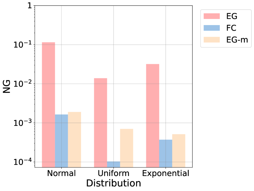
(a) Nash Gap on different context distributions.

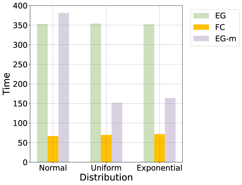
(b) GPU running time on different context distributions.

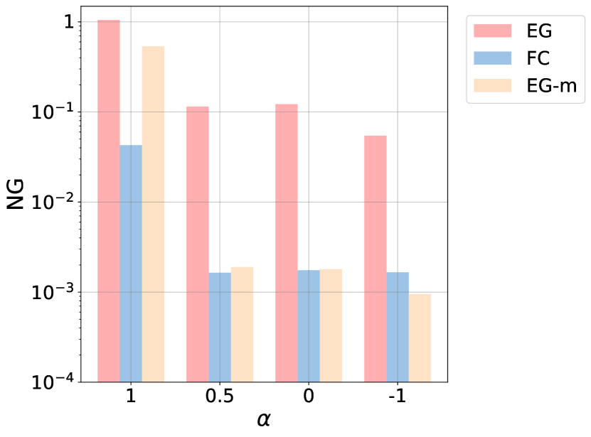
(c) Nash Gap on different CES utilities parameter $\alpha$.

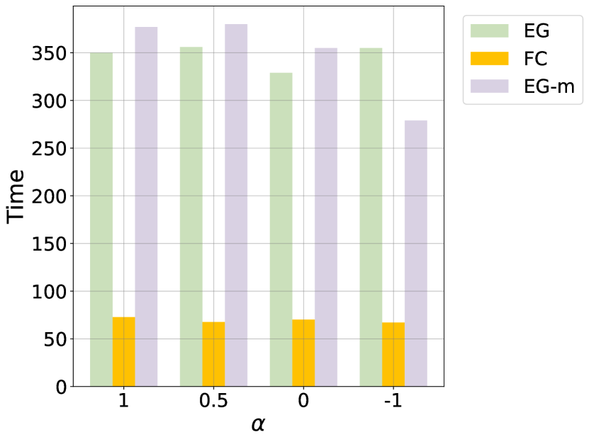
(d) GPU running time on different CES utilities parameter $\alpha$.

Different market scale for MarketFCNet

In this section we ask that how market size (here $n$ and $m$) will have impact on the efficiency of MarketFCNet. We set $m=5,10,20$ and $n=2^{18}=262,114,2^{20}=1,048,576,2^{22}=4,194,304$ as the experimental settings. For each combination of $n$ and $m$, we train MarketFCNet and compared with EG and EG-m, see results in Figure 3(b). As the market size varies, MarketFCNet has almost the same Nash Gap and running time, which shows the robustness of MarketFCNet method over different market sizes. However, as the market size increases, both EG and EG-m have larger Nash Gaps and longer running times, demonstrating that MarketFCNet is more suitable to large-scale contextual market equilibrium computation.

Figure 3: The Nash Gap and GPU running time for different algorithms: MarketFCNet, EG and EG-m. Different colors represent for different algorithm. Market size is chosen as $n=2^{18},2^{20},2^{22}$ buyers and $m=5,10,20$ goods.

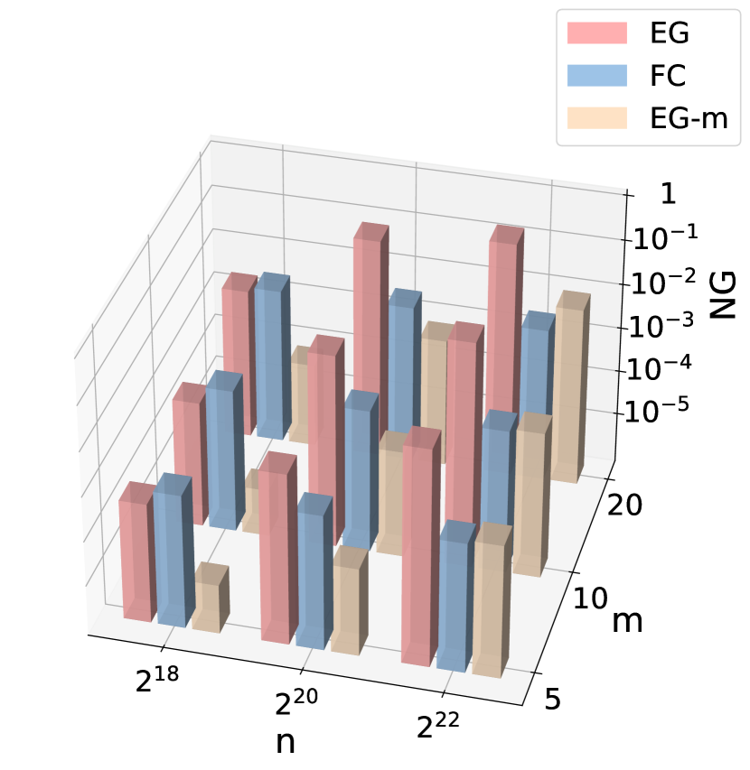
(a) Nash Gap on different market size, $n=2^{18},2^{20},2^{22}$ buyers and $m=5,10,20$ goods.

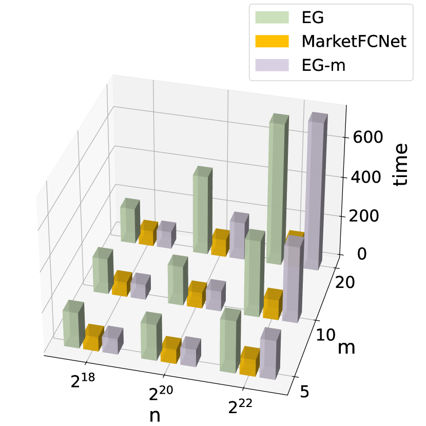
(b) GPU running time on different market size, $n=2^{18},2^{20},2^{22}$ buyers and $m=5,10,20$ goods.

7 Conclusions and Future Work

This paper initiates the problem of large-scale contextual market equilibrium computation from a deep learning perspective. We believe that our approach will pioneer a promising direction for large-scale contextual market equilibrium computation.

For future works, it would be promising to extend these methods to the case when only the number of goods is large, or both the numbers of goods and buyers are large, which stays a blank throughout our works. Since many existing works proposed dynamics for online market equilibrium computation, it’s also promising to extend our approaches to tackle the online market setting with large buyers. Besides, both existing works and ours consider sure budgets and values for buyers, and it would be interesting to extend the fisher market and equilibrium concept when the budgets or values of buyers are stochastic or uncertain.

Appendix A Derivation of Fixed-price Utility for CES Utility Functions

In this section we show the explicit expressions of Fixed-price Utility for CES utility functions.

We first consider the case $\alpha\neq 0,1,-\infty$. The optimization problem for consumer $i$ is:

$$\max_{x_{ij},{j\in[m]}}\quad u_{i}({\bm{x}}_{i})=\left[\sum_{j\in[m]}v^{\alpha}_{ij}x^{\alpha}_{ij}\right]^{1/\alpha}$$ (15)

$$s.t.\quad \sum_{j\in[m]}x_{ij}p_{j}=B_{i}$$ (Budget Constraint)

$$x_{ij}\geq 0$$ (16)

Not hard to verify that in an optimal solution with Equation Budget Constraint, Equation 16 always holds, therefore we omit this constraint in our derivation.

We write the Lagrangian $L({\bm{x}}_{i},\lambda)$

$$L({\bm{x}}_{i},\lambda)=u_{i}({\bm{x}}_{i})+\lambda(B_{i}-\sum_{j\in[m]}x_{ij}p_{j})$$ (17)

By $\frac{\partial L}{\partial x_{ij}}=0$, we have

$$\frac{\partial u_{i}}{\partial x_{ij}^{*}}({\bm{x}}_{i})=\lambda p_{j}$$ (18)

We derive that

$$\frac{\partial u_{i}}{\partial x_{ij}}({\bm{x}}_{i})= \frac{1}{\alpha}\left[\sum_{j\in[m]}v^{\alpha}_{ij}x^{\alpha}_{ij}\right]^{1/\alpha-1}\cdot\alpha v^{\alpha}_{ij}x^{\alpha-1}_{ij}$$ (19)

$$v^{\alpha}_{ij}x^{\alpha-1}_{ij}= cp_{j}\qquad\cdots\text{let $c=\lambda\cdot\left[\sum_{j\in[m]}v^{\alpha}_{ij}x^{\alpha}_{ij}\right]^{1/\alpha-1}$}$$ (20)

$$x_{ij}^{*}= \frac{v_{ij}^{\frac{\alpha}{1-\alpha}}}{c^{\frac{1}{1-\alpha}}\cdot p_{j}^{\frac{1}{1-\alpha}}}$$ (21)

Taking (21) into (Budget Constraint), we get

$$B_{i}= \sum_{j\in[m]}\frac{v_{ij}^{\frac{\alpha}{1-\alpha}}}{c^{\frac{1}{1-\alpha}}}\cdot p_{j}^{-\frac{\alpha}{1-\alpha}}$$ (22)

$$c^{\frac{1}{1-\alpha}}= \frac{1}{B_{i}}\sum_{j\in[m]}\left(\frac{v_{ij}}{p_{j}}\right)^{\frac{\alpha}{1-\alpha}}$$ (23)

Taking Equation 23 into Equation 21, we get

$$x_{ij}^{*}=\frac{v_{ij}^{\frac{\alpha}{1-\alpha}}}{p_{j}^{\frac{1}{1-\alpha}}}\cdot\frac{B_{i}}{c_{0}}$$ (24)

where $c_{0}=\sum_{j\in[m]}\left(\frac{v_{ij}}{p_{j}}\right)^{\frac{\alpha}{1-\alpha}}$

Taking Equation 24 into Equation 15, we finally have

$$u_{i}({\bm{x}}_{i}^{*})= \left[v_{ij}^{\alpha}x_{ij}^{\alpha}\right]^{\frac{1}{\alpha}}$$ (25)

$$= \left[\sum_{j\in[m]}v_{ij}^{\alpha}\frac{v_{ij}^{\frac{\alpha^{2}}{1-\alpha}}}{p_{j}^{\frac{\alpha}{1-\alpha}}}c_{0}^{\alpha}\right]$$

$$= \left[\sum_{j\in[m]}\left(\frac{v_{ij}}{p_{j}}\right)^{\frac{\alpha}{1-\alpha}}c_{0}^{\alpha}\right]$$

$$= B_{i}c_{0}^{\frac{1-\alpha}{\alpha}}$$

$$\log\tilde{u}_{i}({\bm{p}})= \log u_{i}({\bm{x}}_{i}^{*})=\log B_{i}+\frac{1-\alpha}{\alpha}\log c_{0}$$

For $\alpha=1$, by simple arguments we know that consumer will only buy the good that with largest value-per-cost, i.e., $v_{ij}/p_{j}$. Therefore, we have

$$\log\tilde{u}_{i}({\bm{p}})=\log B_{i}+\log\max_{j}\frac{v_{ij}}{p_{j}}$$ (26)

For $\alpha=0$, we have $\log u_{i}({\bm{x}}_{i})=\frac{1}{v_{t}}\sum_{j\in[m]}v_{ij}\log x_{ij}$ where $v_{t}=\sum_{j\in[m]}v_{ij}$.

Similarly, we have

$$cp_{j}= \frac{\partial\log u_{i}}{\partial x_{ij}}=\frac{v_{ij}}{x_{ij}}$$ (27)

$$x_{ij}^{*}= \frac{v_{ij}}{cp_{j}}$$ (28)

By solving budget constraints we have $c=\frac{v_{t}}{B_{i}}$, and therefore, $x_{ij}^{*}=\frac{v_{ij}B_{i}}{p_{j}v_{t}}$ and

$$\log u_{i}({\bm{x}}_{i}^{*})= \frac{1}{v_{t}}\sum_{j\in[m]}(v_{ij}\log\frac{v_{ij}B_{i}}{p_{j}v_{t}})$$ (29)

$$= \log B_{i}+\sum_{j\in[m]}\frac{v_{ij}}{v_{t}}\log\frac{v_{ij}}{p_{j}v_{t}}$$ (30)

For $\alpha=-\infty$, we can easily know that $v_{ij}x_{ij}^{*}\equiv c$ for some $c$. By solving budget constraint we have

$$\sum_{j\in[m]}\frac{cp_{j}}{v_{ij}}=B_{i}$$ (31)

$$c=B_{i}\left(\sum_{j\in[m]}\frac{p_{j}}{v_{ij}}\right)^{-1}$$ (32)

$$\log\tilde{u}_{i}({\bm{p}})=\log c=\log B_{i}-\log\sum_{j\in[m]}\frac{p_{j}}{v_{ij}}$$ (33)

Above all, the log Fixed-price Utility for CES functions is

$$\log\tilde{u}_{i}({\bm{p}})=\begin{cases}\log B_{i}+\max_{j}\log\frac{v_{ij}}{p_{j}}\quad\text{ for $\alpha=1$}\\ \log B_{i}+\sum_{j\in[m]}\frac{v_{ij}}{v_{t}}\log\frac{v_{ij}}{p_{j}v_{t}}\quad\text{ for $\alpha=0$}\\ \log B_{i}-\log\sum_{j\in[m]}\frac{p_{j}}{v_{ij}}\quad\text{ for $\alpha=-\infty$}\\ \log B_{i}+\frac{1-\alpha}{\alpha}\log c_{0}\quad\text{ others}\end{cases}$$ (34)

Appendix B Omitted Proofs

B.1 Proof of Proposition 3.2

We consider Lagrangian multipliers ${\bm{p}}$ and use the KKT condition. The Lagrangian becomes

$$L({\bm{p}},{\bm{x}})=\sum_{i}B_{i}\log u_{i}({\bm{x}}_{i})-\sum_{j}p_{j}(\sum_{i}x_{ij}-Y_{j})$$ (35)

and the partial derivative of $x_{ij}$ is

$$\frac{\partial L({\bm{p}},{\bm{x}}_{i})}{\partial x_{ij}}=\frac{B_{i}}{u_{i}({\bm{x}}_{i})}\frac{\partial u_{i}}{\partial x_{ij}}-p_{j}$$ (36)

By complementary slackness of $x_{ij}\geq 0$, we have

$$\frac{B_{i}}{u_{i}({\bm{x}}_{i})}\frac{\partial u_{i}}{\partial x_{ij}}\leq p_{j}\text{ for all $i$}$$ (37)

By theorem 3.1, we know that if $({\bm{x}},{\bm{p}})$ is a market equilibrium, we must have $u_{i}({\bm{x}}_{i})>0$ for all $i$, and by condition in Proposition 3.2, we can always select buyer $i$ such that $\frac{\partial u_{i}}{\partial x_{ij}}>0$. Therefore, we have $p_{j}>0$.

As a consequence, $p_{j}>0$ indicates that $\sum_{j}x_{ij}=V_{j}$ by market clearance condition.

B.2 Proof of Proposition 5.4

Consider the market equilibrium condition $\langle{\bm{p}}^{*},{\bm{x}}^{*}_{i}\rangle=B_{i}$, we have $\sum_{j}p_{j}x_{ij}=B_{i}$. sum over this expression, we have $\sum_{i}\sum_{j}p_{j}x_{ij}=\sum_{i}B_{i}$. Then, $\sum_{j}p_{j}\sum_{i}x_{ij}=\sum_{i}B_{i}$. Notice that we have $\sum_{i=1}^{n}x_{ij}=Y_{j}$ in market equilibrium, so $\sum_{j}p_{j}Y_{j}=\sum_{i}B_{i}$, that completes the proof.

B.3 Proof of Theorem 5.5

Proof of Theorem 5.5.

Denote $({\bm{x}},{\bm{p}})$ as the market equilibrium, ${\bm{p}}$ as the price for goods and ${\bm{x}}^{*}_{i}({\bm{p}})$ as the optimal consumption set of buyer $i$ when the price is ${\bm{p}}$.

We have following equation:

$$\sum_{j}x_{ij}p_{j}= B_{i}$$ (38)

$${\bm{x}}_{i}\in {\bm{x}}^{*}_{i}({\bm{p}})$$ (39)

$$\sum_{i\in[n]}x_{ij}= Y_{j}$$ (40)

$$u_{i}({\bm{p}})= u_{i}({\bm{x}}_{i}),\ \forall{\bm{p}}\in\mathbb{R}^{m}_{+},\ \forall{\bm{x}}_{i}\in{\bm{x}}^{*}_{i}({\bm{p}})$$ (41)

From Proposition 5.4 we know $\sum_{i\in[n]}B_{i}=\sum_{j\in[m]}Y_{j}p_{j}$.

Let ${\bm{p}}^{\prime}$ be some price for items such that $\sum_{j\in[m]}Y_{j}{\bm{p}}^{\prime}_{j}=\sum_{i\in[n]}B_{i}$. Let ${\bm{x}}^{\prime}_{i}\in{\bm{x}}^{*}_{i}({\bm{p}}^{\prime})$ and $B^{\prime}_{i}=\langle{\bm{p}}^{\prime},{\bm{x}}_{i}\rangle$. We know that

$$\sum_{i\in[n]}B^{\prime}_{i}=\langle{\bm{p}}^{\prime},\sum_{i\in[n]}{\bm{x}}_{i}\rangle=\langle{\bm{p}}^{\prime},\bm{Y}\rangle=\sum_{i\in[n]}B_{i}$$ (42)

For consumer $i$, ${\bm{x}}_{i}$ costs $B^{\prime}_{i}$ at price ${\bm{p}}^{\prime}$, thus $\frac{B_{i}}{B^{\prime}_{i}}{\bm{x}}_{i}$ costs $B_{i}$ at price ${\bm{p}}^{\prime}$. Besides, ${\bm{x}}^{\prime}_{i}$ also costs $B_{i}$ for price ${\bm{p}}^{\prime}$, and ${\bm{x}}^{\prime}$ is the optimal consumption for buyer $i$. Then we have

$$u_{i}({\bm{p}}^{\prime})=u_{i}({\bm{x}}^{\prime}_{i})\geq u_{i}(\frac{B_{i}}{B^{\prime}_{i}}{\bm{x}}_{i})=\frac{B_{i}}{B^{\prime}_{i}}u_{i}({\bm{x}}_{i})$$ (43)

where the last equation is from the homogeneity(with degree 1) of utility function.

Taking logarithm and weighted sum with $B_{i}$, we have

$$\sum_{i\in[n]}B_{i}\log u_{i}({\bm{p}}^{\prime})\geq\sum_{i\in[n]}B_{i}\log\frac{B_{i}}{B^{\prime}_{i}}+\sum_{i\in[n]}B_{i}\log u_{i}({\bm{x}}_{i})$$ (44)

Take $B_{\mathrm{total}}=\sum_{i\in[n]}B_{i}$, the first term in RHS becomes

$$\sum_{i\in[n]}B_{i}\log\frac{B_{i}}{B^{\prime}_{i}}$$ (45)

$$= B_{\mathrm{total}}\sum_{i\in[n]}\left(\frac{B_{i}}{B_{\mathrm{total}}}\log\frac{B_{i}/B_{\mathrm{total}}}{B^{\prime}_{i}/B_{\mathrm{total}}}\right)$$ (46)

$$= B_{\mathrm{total}}\cdot\text{KL}(\frac{\bm{B}}{B_{\mathrm{total}}}||\frac{\bm{B^{\prime}}}{B_{\mathrm{total}}})$$ (47)

$$\geq 0$$ (48)

Therefore,

$$\sum_{i\in[n]}B_{i}\log u_{i}({\bm{p}}^{\prime})\geq\sum_{i\in[n]}B_{i}\log u_{i}({\bm{x}}_{i})$$ (49)

For ${\bm{x}}^{\prime}$ that satisfies market clearance, by optimality of EG program(EG), we have

$$\sum_{i\in[n]}B_{i}\log u_{i}({\bm{x}}_{i})\geq\sum_{i\in[n]}B_{i}\log u_{i}({\bm{x}}^{\prime}_{i})$$ (50)

Equation 49 and Equation 50 together complete the proof of the first part.

If $({\bm{x}},{\bm{p}})$ constitutes a market equilibrium, it’s obvious that $\mathrm{LFW}({\bm{p}})$ and $\mathrm{LNW}({\bm{x}})$ are identical, therefore $\mathrm{NG}({\bm{x}},{\bm{p}})=0$.

On the other hand, if $({\bm{x}},{\bm{p}})$ is not a market equilibrium, but $\mathrm{NG}({\bm{x}},{\bm{p}})=0$, it means that the KL convergence term must equal to 0, and $B_{i}=B^{\prime}_{i}$ for all $i$, which means that ${\bm{x}}_{i}$ costs buyer $i$ with money $B_{i}$ and ${\bm{x}}_{i}$ are in the consumption set of buyer $i$. Since $({\bm{x}},{\bm{p}})$ is not a market equilibrium, there is at least one buyer that can choose a better allocation ${\bm{x}}^{\prime}_{i}$ to improve her utility, therefore improve $\mathrm{LFW}({\bm{p}})$, and it cannot be the case that $\mathrm{LFW}({\bm{p}})=\mathrm{LNW}({\bm{x}})$, which makes a contradiction.

∎

B.4 Proof of Proposition 5.6

We leave the formal presentation of Proposition 5.6 and proofs to three theorems below.

Lemma B.1.

Assume that $u_{i}({\bm{x}}_{i})$ is twice differentiable and denote $H({\bm{x}}_{i})$ as the Hessian matrix of $u_{i}({\bm{x}}_{i})$. If following hold:

• $H({\bm{x}}_{i}^{*})$ has rank $m-1$

• $||{\bm{x}}_{i}-{\bm{x}}_{i}^{*}||=\varepsilon$ for some $i$

• ${\bm{x}}_{i}^{*}>\mathbf{0}$

then we have $\mathrm{OPT}-\mathrm{LNW}({\bm{x}})=\Omega(\varepsilon^{2})$.

Lemma B.2.

Denote $\tilde{u}_{i}({\bm{p}},B_{i})$ and ${\bm{x}}_{i}^{*}({\bm{p}},B_{i})$ as the maximum utility buyer $i$ can get and the corresponding consumption for buyer $i$ when her budget is $B_{i}$ and prices are ${\bm{p}}$. If following hold:

• $||{\bm{p}}-{\bm{p}}^{*}||=\varepsilon$

• ${\bm{x}}_{i}^{*}({\bm{p}},B_{i})$ is differentiable with ${\bm{p}}$.

• $H_{X}\coloneqq(\sum_{i\in[n]}\frac{\partial x_{ij}^{*}}{\partial p_{k}}({\bm{p}}^{*},B_{i}))_{j,k\in[m]}$ has full rank.

then we have $LFW({\bm{p}})-OPT=\Omega(\varepsilon^{2})$.

Remark B.3.

It’s worth notice that $H({\bm{x}}_{i}^{*})$ can not has full rank $m$, since $u_{i}({\bm{x}})$ is assumed to be homogeneous and thus linear in the direction ${\bm{x}}$. Therefore, we have $H({\bm{x}}_{i}){\bm{x}}_{i}=\mathbf{0}$ for all ${\bm{x}}_{i}$.

Let $C_{i}=\{{\bm{x}}_{i}\in\mathbb{R}_{+}^{m}:\langle{\bm{p}},{\bm{x}}_{i}\rangle=B_{i}\}$ be the consumption set of buyer $i$, since ${\bm{x}}_{i}$ can not be parallel with $C_{i}$, the condition that $H({\bm{x}}_{i}^{*})$ has rank $m-1$ means that, $H({\bm{x}}_{i})$ is strongly concave at point ${\bm{x}}_{i}^{*}$ on the consumption set $C_{i}$.

Besides, we emphasize that the conditions in Lemma B.1 and Lemma B.2 are satisfied for CES utility with $\alpha<1$.

Corollary B.4.

Under the assumptions in Lemma B.1 and Lemma B.2, if $\mathrm{NG}({\bm{x}},{\bm{p}})=\varepsilon$, we have:

• $||{\bm{p}}-{\bm{p}}^{*}||=O(\sqrt{\varepsilon})$

• $||{\bm{x}}_{i}-{\bm{x}}_{i}^{*}||=O(\sqrt{\varepsilon})$ for all $i$

Proof of Corollary B.4.

A direct inference from Lemma B.1 and Lemma B.2, notice that $\mathrm{NG}=\varepsilon$ indicates that $\mathrm{OPT}-\mathrm{LNW}({\bm{x}})\leq\varepsilon$ and $\mathrm{LFW}({\bm{p}})-\mathrm{OPT}\leq\varepsilon$. ∎

Corollary B.4 states that, for a pair of $({\bm{x}},{\bm{p}})$ that satisfy market clearance and price constraints, a small Nash Gap indicates that the point $({\bm{x}},{\bm{p}})$ is close to the equilibrium point $({\bm{x}}^{*},{\bm{p}}^{*})$, in the sense of Euclidean distance.

Lemma B.5.

Assume following hold:

• buyers have same utilities at ${\bm{x}}^{*}$, i.e. $u_{i}({\bm{x}}_{i}^{*})=u_{j}({\bm{x}}_{j}^{*})\equiv c$ for all $i,~{}j$

• $||{\bm{x}}_{i}-{\bm{x}}_{i}^{*}||\leq\varepsilon$ for all $i$

then, we have $|\mathrm{WSW}({\bm{x}})-\mathrm{WSW}({\bm{x}}^{*})|=O(\varepsilon^{2})$.

Remark B.6.

These conditions can be held when buyers are homogeneous, i.e., $B_{i}=B_{j}$ and $u_{i}({\bm{x}})=u_{j}({\bm{x}})$ for all $i,j,{\bm{x}}\in\mathbb{R}^{m}_{+}$. Besides, consider buyers with same budgets, these conditions can also be held if the market has some “equivariance property”, e.g., there is a $n$-cycle permutation of buyers $\rho$ and permutation of goods $\tau$, such that $u_{i}({\bm{x}}_{i})=u_{\rho(i)}(\tau({\bm{x}}_{\rho(i)}))$ for all $i$ and $\tau(Y_{1},...,Y_{m})=(Y_{1},...,Y_{m})$.

Corollary B.7.

Under the assumptions in Lemma B.1 and Lemma B.5, if $\mathrm{NG}({\bm{x}},{\bm{p}})=\varepsilon$, we have

• $|\mathrm{WSW}({\bm{x}})-\mathrm{WSW}({\bm{x}}^{*})|=O(\varepsilon)$.

Proof.

A direct inference from Lemma B.1 and Lemma B.5. ∎

B.4.1 Proof of Lemma B.1

Proof of Lemma B.1.

We observe that

$$\mathrm{OPT}-\mathrm{LNW}({\bm{x}})=\sum_{i\in[n]}B_{i}\left[\log u_{i}({\bm{x}}_{i}^{*})-\log u_{i}({\bm{x}}_{i})\right]$$

Consider the Taylor expansion of $\log u_{i}({\bm{x}}_{i})$ and $u_{i}({\bm{x}}_{i})$:

$$\log u_{i}({\bm{x}}_{i})= \log u_{i}({\bm{x}}_{i}^{*})+\frac{1}{u_{i}({\bm{x}}_{i}^{*})}(u_{i}({\bm{x}}_{i})-u_{i}({\bm{x}}_{i}^{*}))$$

$$- \frac{1}{2u_{i}({\bm{x}}_{i}^{*})^{2}}(u_{i}({\bm{x}}_{i})-u_{i}({\bm{x}}_{i}^{*}))^{2}$$

$$+ O((u_{i}({\bm{x}}_{i})-u_{i}({\bm{x}}_{i}^{*}))^{3})$$

$$u_{i}({\bm{x}}_{i})= u_{i}({\bm{x}}_{i}^{*})+\frac{\partial u_{i}}{\partial{\bm{x}}_{i}}({\bm{x}}_{i}^{*})({\bm{x}}_{i}-{\bm{x}}_{i}^{*})$$

$$+ \frac{1}{2}({\bm{x}}_{i}-{\bm{x}}_{i}^{*})^{T}H({\bm{x}}_{i}^{*})({\bm{x}}_{i}-{\bm{x}}_{i}^{*})+O(||{\bm{x}}_{i}-{\bm{x}}_{i}^{*}||^{3})$$

Notice that $||{\bm{x}}_{i}-{\bm{x}}_{i}^{*}||=\varepsilon$, we have

$$\log u_{i}({\bm{x}}_{i})= \log u_{i}({\bm{x}}_{i}^{*})$$

$$+ \frac{1}{u_{i}({\bm{x}}_{i}^{*})}[\frac{\partial u_{i}}{\partial x_{i}}({\bm{x}}_{i}^{*})({\bm{x}}_{i}-{\bm{x}}_{i}^{*})\cdots\varepsilon\text{ term}$$ (51)

$$+ \frac{1}{2}({\bm{x}}_{i}-{\bm{x}}_{i}^{*})^{T}H({\bm{x}}_{i}^{*})({\bm{x}}_{i}-{\bm{x}}_{i}^{*})]\cdots\varepsilon^{2}\text{ term}$$ (52)

$$- \frac{1}{2u_{i}({\bm{x}}_{i}^{*})^{2}}\left(\frac{\partial u_{i}}{\partial{\bm{x}}_{i}}({\bm{x}}_{i}^{*})({\bm{x}}_{i}-{\bm{x}}_{i}^{*})\right)^{2}\cdots\varepsilon^{2}\text{ term}$$ (53)

$$+ O(\varepsilon^{3})$$

We next deal with Equation 51 to Equation 53 separately.

Derivation of Equation 51

Since ${\bm{x}}_{i}^{*}$ solves the buyer $i$’s problem, we must have

$$\frac{\partial u_{i}}{\partial x_{i}}({\bm{x}}_{i}^{*})=\lambda_{i}{\bm{p}}^{*}$$ (54)

where $\lambda_{i}$ is the Lagrangian Multipliers for buyer $i$.

We also know that $u_{i}({\bm{x}}_{i})$ is homogeneous with degree 1, by Euler formula, we derive

$$\langle\frac{\partial u_{i}}{\partial x_{i}}({\bm{x}}_{i}),{\bm{x}}_{i}\rangle=u_{i}({\bm{x}}_{i})$$ (55)

Combine Equation 54 and Equation 55 and take ${\bm{x}}_{i}={\bm{x}}_{i}^{*}$, we derive

$$\lambda_{i}\langle{\bm{p}}^{*},{\bm{x}}_{i}^{*}\rangle= u_{i}({\bm{x}}_{i}^{*})$$

$$\lambda_{i}= \frac{u_{i}({\bm{x}}_{i}^{*})}{B_{i}}$$

$$\frac{\partial u_{i}}{\partial x_{i}}({\bm{x}}_{i}^{*})= \frac{u_{i}({\bm{x}}_{i}^{*})}{B_{i}}{\bm{p}}^{*}$$

Sum up over $i$ for Equation 51, we have

$$\sum_{i\in[n]}B_{i}\frac{1}{u_{i}({\bm{x}}_{i}^{*})}\frac{\partial u_{i}}{\partial x_{i}}({\bm{x}}_{i}^{*})({\bm{x}}_{i}-{\bm{x}}_{i}^{*})$$ (56)

$$= {\bm{p}}\sum_{i\in[n]}({\bm{x}}_{i}-{\bm{x}}_{i}^{*})$$

$$= 0\cdots\text{by market clearance}$$

Derivation of Equation 52 and Equation 53

Combining Equation 52 and Equation 53, we have

$$\frac{B_{i}}{2u_{i}({\bm{x}}_{i}^{*})}({\bm{x}}_{i}-{\bm{x}}_{i}^{*})^{T}H({\bm{x}}_{i}^{*})({\bm{x}}_{i}-{\bm{x}}_{i}^{*})-\frac{1}{2B_{i}}({\bm{x}}_{i}-{\bm{x}}_{i}^{*})^{T}({\bm{p}}^{*}{\bm{p}}^{*T})({\bm{x}}_{i}-{\bm{x}}_{i}^{*})$$

$$= \frac{1}{2B_{i}}({\bm{x}}_{i}-{\bm{x}}_{i}^{*})^{T}(\frac{B_{i}^{2}}{u_{i}({\bm{x}}_{i}^{*})}H({\bm{x}}_{i}^{*})-{\bm{p}}^{*}{\bm{p}}^{*T})({\bm{x}}_{i}-{\bm{x}}_{i}^{*})$$

Denote $H_{0}({\bm{x}}_{i}^{*})=\frac{B_{i}^{2}}{u_{i}({\bm{x}}_{i}^{*})}H({\bm{x}}_{i}^{*})-{\bm{p}}^{*}{\bm{p}}^{*T}$, next we assert that $H_{0}({\bm{x}}_{i}^{*})$ is negative definite.

Since $H({\bm{x}}_{i}^{*})$ and $-{\bm{p}}^{*}{\bm{p}}^{*T}$ are negative semi-definite, $H_{0}({\bm{x}}_{i}^{*})$ must be negative semi-definite with $\mathrm{rank}(H_{0}({\bm{x}}_{i}^{*}))\geq m-1$.

Let $\lambda_{1}\leq\lambda_{2}\leq\dots\leq\lambda_{m-1}<\lambda_{m}=0$ be eigenvalues and $v_{1},...,v_{n}={\bm{x}}_{i}^{*}$ be eigenvectors of $H({\bm{x}}_{i}^{*})$. If $\mathrm{rank}(H_{0}({\bm{x}}_{i}^{*}))=m-1$, it means that ${\bm{x}}_{i}^{*}$ has to be eigenvectors of $-{\bm{p}}^{*}{\bm{p}}^{*T}$ with eigenvalue $0$. However, we have $-{\bm{p}}^{*}{\bm{p}}^{*T}{\bm{x}}_{i}^{*}=-B_{i}{\bm{p}}^{*}\neq 0$, which leads to a contradiction.

Therefore, we have $\mathrm{rank}(H_{0}({\bm{x}}_{i}^{*}))=m$ and $H_{0}({\bm{x}}_{i}^{*})$ is negative definite, we denote $\lambda^{i}_{1}\leq...,\leq\lambda^{i}_{n}<0$ as the eigenvalues of $H_{0}({\bm{x}}_{i}^{*})$, and $k$ as the universal lower bound for $|\lambda^{i}_{n}|$, then we have that,

$$\frac{1}{2}({\bm{x}}_{i}-{\bm{x}}_{i}^{*})^{T}H_{0}({\bm{x}}_{i}^{*})({\bm{x}}_{i}-{\bm{x}}_{i}^{*})\leq-\frac{k}{2}\varepsilon^{2}$$ (57)

By combining Equation 56 and Equation 57, we have

$$\mathrm{OPT}-\mathrm{LNW}({\bm{x}})= -\sum_{i\in[n]}B_{i}\left[\frac{1}{2B_{i}}({\bm{x}}_{i}-{\bm{x}}_{i}^{*})^{T}H_{0}({\bm{x}}_{i}^{*})({\bm{x}}_{i}-{\bm{x}}_{i}^{*})\right]+O(\varepsilon^{3})$$ (58)

$$\geq \frac{k}{2}\varepsilon^{2}+O(\varepsilon^{3})$$

$$= \Omega(\varepsilon^{2})$$

∎

B.4.2 Proof of Lemma B.2

Proof of Lemma B.2.

The proof is similar with Section B.4.1 by using Taylor expansion technique. Before that, we first derive some identities.

By Roy’s identity, we have

$$\frac{\partial\tilde{u_{i}}}{\partial p_{j}}({\bm{p}},B_{i})=-x_{ij}^{*}({\bm{p}},B_{i})\frac{\partial\tilde{u}_{i}}{\partial B_{i}}({\bm{p}},B_{i})$$

Since $u({\bm{x}}_{i})$ is homogeneous with ${\bm{x}}_{i}$, it’s easy to derive that

$$\frac{\partial\tilde{u}_{i}}{\partial B_{i}}({\bm{p}},B_{i})=\frac{\tilde{u}_{i}({\bm{p}},B_{i})}{B_{i}}$$

Above all,

$$\frac{\partial\tilde{u_{i}}}{\partial p_{j}}({\bm{p}},B_{i})=-\frac{1}{B_{i}}x_{ij}^{*}({\bm{p}},B_{i})\tilde{u}_{i}({\bm{p}},B_{i})$$

Besides,

$$\frac{\partial^{2}\tilde{u_{i}}}{\partial p_{j}\partial p_{k}}({\bm{p}},B_{i})= \frac{1}{B_{i}^{2}}x_{ij}^{*}({\bm{p}},B_{i})x_{ik}^{*}({\bm{p}},B_{i})\tilde{u}_{i}({\bm{p}},B_{i})$$

$$- \frac{1}{B_{i}}\frac{x_{ij}^{*}({\bm{p}},B_{i})}{\partial p_{k}}\tilde{u}_{i}({\bm{p}},B_{i})$$

Next we consider the Taylor expansion,

$$\log\tilde{u}_{i}({\bm{p}})= \log\tilde{u}_{i}({\bm{p}}^{*})$$

$$+ \frac{1}{\tilde{u}_{i}({\bm{p}}^{*})}[\frac{\partial\tilde{u}_{i}}{\partial{\bm{p}}}({\bm{p}}^{*})({\bm{p}}-{\bm{p}}^{*})\cdots\varepsilon\text{ term}$$ (59)

$$+ \frac{1}{2}({\bm{p}}-{\bm{p}}^{*})^{T}H_{p}({\bm{p}}-{\bm{p}}^{*})]\cdots\varepsilon^{2}\text{ term}$$ (60)

$$- \frac{1}{2\tilde{u}_{i}({\bm{p}}^{*})^{2}}\left[\frac{\partial\tilde{u}_{i}}{\partial{\bm{p}}}({\bm{p}}^{*})({\bm{p}}-{\bm{p}}^{*})\right]^{2}\cdots\varepsilon^{2}\text{ term}$$ (61)

$$+ O(\varepsilon^{3})$$

where $H_{p}$ is the Hessian matrix for $\tilde{u}_{i}({\bm{p}})$.

Derivation of Equation 59

We have

$$\sum_{i\in[n]}B_{i}\frac{1}{\tilde{u}_{i}({\bm{p}}^{*})}\langle\frac{\partial\tilde{u}_{i}}{\partial{\bm{p}}}({\bm{p}}^{*}),({\bm{p}}-{\bm{p}}^{*})\rangle$$

$$= \sum_{i\in[n]}\langle{\bm{x}}_{i}^{*},({\bm{p}}-{\bm{p}}^{*})\rangle$$

$$= \langle\mathbf{1},({\bm{p}}-{\bm{p}}^{*})\rangle\cdots\text{by market clearance}$$

$$= 0\cdots\text{by price constraints}$$

Derivation of Equation 60 and Equation 61

These expressions become

$$\frac{1}{2\tilde{u}_{i}({\bm{p}}^{*})}[\frac{1}{B_{i}^{2}}\tilde{u}_{i}({\bm{p}}^{*})\langle{\bm{x}}_{i}^{*},{\bm{p}}-{\bm{p}}^{*}\rangle^{2}-\frac{1}{B_{i}}\tilde{u}_{i}({\bm{p}}^{*})({\bm{p}}-{\bm{p}}^{*})^{T}(\frac{\partial x_{ij}^{*}}{\partial p_{k}}({\bm{p}}^{*},B_{i}))_{j,k\in[m]}({\bm{p}}-{\bm{p}}^{*})]$$

$$- \frac{1}{2\tilde{u}_{i}({\bm{p}}^{*})^{2}}\frac{\tilde{u}_{i}({\bm{p}}^{*})^{2}}{B_{i}^{2}}\langle{\bm{x}}_{i}^{*},{\bm{p}}-{\bm{p}}^{*}\rangle^{2}$$

$$= \frac{1}{2B_{i}}({\bm{p}}-{\bm{p}}^{*})^{T}(\frac{\partial x_{ij}^{*}}{\partial p_{k}}({\bm{p}}^{*},B_{i}))_{j,k\in[m]}({\bm{p}}-{\bm{p}}^{*})$$

Summing up over $i$, we derive that

$$\mathrm{LFW}({\bm{p}})-\mathrm{OPT}= \sum_{i\in[n]}B_{i}\frac{1}{2B_{i}}({\bm{p}}-{\bm{p}}^{*})^{T}(\frac{\partial x_{ij}^{*}}{\partial p_{k}}({\bm{p}}^{*},B_{i}))_{j,k\in[m]}({\bm{p}}-{\bm{p}}^{*})+O(\varepsilon^{3})$$

$$= \frac{1}{2}({\bm{p}}-{\bm{p}}^{*})^{T}H_{X}({\bm{p}}-{\bm{p}}^{*})+O(\varepsilon^{3})$$

Since ${\bm{p}}^{*}$ gets the minimum of $\mathrm{LFW}({\bm{p}})$, we must have that $H_{X}$ is positive semi-definite. Together with $H_{X}$ has full rank, we know that $H_{X}$ is positive definite. Denote $\lambda_{m}$ as the minimum eigenvalues of $H_{X}$, we have

$$\mathrm{LFW}({\bm{p}})-\mathrm{OPT}\geq \frac{\varepsilon^{2}\lambda_{m}}{2}+O(\varepsilon^{3})$$

$$= \Omega(\varepsilon^{2})$$

∎

B.4.3 Proof of Lemma B.5

Proof of Lemma B.5.

Notice that

$$\mathrm{WSW}({\bm{x}})=\mathrm{WSW}({\bm{x}}^{*})+\sum_{i\in[n]}\langle\frac{\partial\mathrm{WSW}}{\partial{\bm{x}}_{i}}({\bm{x}}_{i}^{*}),({\bm{x}}_{i}-{\bm{x}}_{i}^{*})\rangle+O(\varepsilon^{2})$$

We have

$$\frac{\partial\mathrm{WSW}}{\partial{\bm{x}}_{i}}({\bm{x}}_{i}^{*})$$

$$= B_{i}\frac{\partial u_{i}}{\partial{\bm{x}}_{i}}({\bm{x}}_{i}^{*})$$

$$= B_{i}\frac{u_{i}({\bm{x}}_{i}^{*})}{B_{i}}{\bm{p}}^{*}$$

$$= c{\bm{p}}^{*}$$

Therefore,

$$\mathrm{WSW}({\bm{x}})= \mathrm{WSW}({\bm{x}}^{*})+\sum_{i\in[n]}c\langle{\bm{p}}^{*},{\bm{x}}_{i}-{\bm{x}}_{i}^{*}\rangle+O(\varepsilon^{2})$$

$$= \mathrm{WSW}({\bm{x}}^{*})+O(\varepsilon^{2})\cdots\text{market clearance}$$

which completes the proof.

∎

Appendix C Additional Experiments Details

C.1 More about baselines

EG program solver (abbreviated as EG)

We propose the first baseline algorithm EG. Recall the Eisenberg-Gale convex program(EG):

$$\max\quad\frac{1}{n}\sum_{i=1}^{n}B_{i}\log u_{i}({\bm{x}}_{i})\quad{\rm s.t.}\ \frac{1}{n}\sum_{i=1}^{n}x_{ij}=1,\ x\geq 0.$$ (62)

We use the network module in pytorch to represent the parameters ${\bm{x}}\in\mathbb{R}^{n\times m}_{+}$, and softplus activation function to satisfy $x\geq 0$ automatedly. We use gradient ascent algorithm to optimize the parameters ${\bm{x}}$. For constraint $\frac{1}{n}\sum_{i\in[n]}x_{ij}=1$, we introduce Lagrangian multipliers $\lambda_{j}$ and minimize the Lagrangian:

$$\mathcal{L}_{\rho}({\bm{x}};\bm{\lambda})= -\frac{1}{n}\sum_{i\in[n]}B_{i}\log u_{i}({\bm{x}}_{i})+\sum_{j\in[m]}\lambda_{j}\left(\frac{1}{n}\sum_{i\in[n]}x_{ij}-1\right)$$ (63)

$$+ \frac{\rho}{2}\sum_{j\in[m]}\left(\frac{1}{n}\sum_{i\in[n]}x_{ij}-1\right)^{2}$$ (64)

The updates of $\bm{\lambda}$ is $\lambda_{j}\leftarrow\lambda_{j}+\beta_{t}\rho\left(\frac{1}{n}\sum_{i\in[n]}x_{ij}-1\right)$, here $\beta_{t}$ is step size, which is identical with that in MarketFCNet. The algorithm returns the final $({\bm{x}},\bm{\lambda})$ as the approximated market equilibrium.

EG program solver with momentum (abbreviated as EG-m)

The program to solve is exactly same with that in EG. The only difference is that we use gradient ascent with momentum to optimize the parameters ${\bm{x}}$.

C.2 More Experimental Details

Without special specification, we use the experiment settings as follows. All experiments are conducted in one RTX 4090 graphics cards using 16 CPUs or 1 GPU. We set dimension of representations of buyers and goods to be $d=5$. Each elements in representation is i.i.d from $\mathcal{N}(0,1)$ for normal distribution (default) contexts, $U[0,1]$ for uniform distribution contexts and $Exp(1)$ for exponential distribution contexts. Budget is generated with $B(b)=||b||_{2}$, and valuation in utility function is generated with $v(b,g)=\mathrm{softplus}(\langle b,g\rangle)$, where $\mathrm{softplus}(x)=\log(1+\exp(x))$ is a smoothing function that maps each real number to be positive. $\alpha$ in CES utility are chosen to be 0.5 by default. MarketFCNet is designed as a fully connected network with depth 5 and width 256 per layer. $\rho$ is chosen to be 0.2 in Augmented Lagrange Multiplier Method and the step size $\beta_{t}$ is chosen to be $\frac{1}{\sqrt{t}}$. We choose $K=100$ as inner iteration for each epoch, and training for $30$ epochs in MarketFCNet. For EG and EG-m baselines, we choose the inner iteration $K=1000$ when $n>1000$ and $K=100$ when $n\leq 1000$ for each epoch. Baselines are enssembled with early stopping as long as $\mathrm{NG}$ is lower than $10^{-3}$. Both baselines are optimized for $30$ epochs in total.

We use Adam optimizer and learning rate $1e-4$ to optimize the allocation network in MarketFCNet. When computing $\Delta\lambda_{j}$ in MarketFCNet, we directly compute $\Delta\lambda_{j}$ rather than generate an unbiased estimator, since it does not cost too much to consider all buyers for one time. For those baselines, we use gradient descent to optimize the parameters following existing works, and the step size is fine-tuned to be $1e+2$ for $\alpha=1$, $n>1000$; $1e+3$ for $\alpha<1$, $n>1000$ and $1$ for $\alpha<1,\ n\leq 1000$ and $0.1$ for $\alpha=1,\ n\leq 1000$ for better performances of the baselines. Since that Lagrangian multipliers $\lambda\leq 0$ will indicate an illegal Nash Gap measure, therefore, we hard code EG algorithm such that it will only return a result when it satisfies that the price $\lambda_{j}>0$ for all good j. All baselines are run in GPU when $n>1000$ and CPU when $n\leq 1000$.

References

• Amari [1993] Shun-ichi Amari. Backpropagation and stochastic gradient descent method. Neurocomputing, 5(4-5):185–196, 1993.
• Arrow [1951] Kenneth J Arrow. An extension of the basic theorems of classical welfare economics. In Proceedings of the second Berkeley symposium on mathematical statistics and probability, volume 2, pages 507–533. University of California Press, 1951.
• Arrow and Debreu [1954] Kenneth J Arrow and Gerard Debreu. Existence of an equilibrium for a competitive economy. Econometrica: Journal of the Econometric Society, pages 265–290, 1954.
• Arrow et al. [1961] Kenneth J Arrow, Hollis B Chenery, Bagicha S Minhas, and Robert M Solow. Capital-labor substitution and economic efficiency. The review of Economics and Statistics, pages 225–250, 1961.
• Balseiro et al. [2023] Santiago Balseiro, Christian Kroer, and Rachitesh Kumar. Contextual standard auctions with budgets: Revenue equivalence and efficiency guarantees. Management Science, 69(11):6837–6854, 2023.
• Banerjee et al. [2022] Siddhartha Banerjee, Vasilis Gkatzelis, Artur Gorokh, and Billy Jin. Online nash social welfare maximization with predictions. In Proceedings of the 2022 Annual ACM-SIAM Symposium on Discrete Algorithms (SODA), pages 1–19. SIAM, 2022.
• Bengio et al. [2009] Yoshua Bengio, Jérôme Louradour, Ronan Collobert, and Jason Weston. Curriculum learning. In Proceedings of the 26th annual international conference on machine learning, pages 41–48, 2009.
• Bottou [2010] Léon Bottou. Large-scale machine learning with stochastic gradient descent. In Proceedings of COMPSTAT’2010: 19th International Conference on Computational StatisticsParis France, August 22-27, 2010 Keynote, Invited and Contributed Papers, pages 177–186. Springer, 2010.
• Brânzei et al. [2014] Simina Brânzei, Yiling Chen, Xiaotie Deng, Aris Filos-Ratsikas, Søren Frederiksen, and Jie Zhang. The fisher market game: Equilibrium and welfare. In Proceedings of the AAAI Conference on Artificial Intelligence, volume 28, 2014.
• Brogaard et al. [2014] Jonathan Brogaard, Terrence Hendershott, and Ryan Riordan. High-frequency trading and price discovery. The Review of Financial Studies, 27(8):2267–2306, 2014.
• Budish [2011] Eric Budish. The combinatorial assignment problem: Approximate competitive equilibrium from equal incomes. Journal of Political Economy, 119(6):1061–1103, 2011.
• Cheung et al. [2018] Yun Kuen Cheung, Richard Cole, and Yixin Tao. Dynamics of distributed updating in fisher markets. In Proceedings of the 2018 ACM Conference on Economics and Computation, pages 351–368, 2018.
• Cole and Fleischer [2008] Richard Cole and Lisa Fleischer. Fast-converging tatonnement algorithms for one-time and ongoing market problems. In Proceedings of the Fortieth Annual ACM Symposium on Theory of Computing, pages 315–324, 2008.
• Cole et al. [2017] Richard Cole, Nikhil Devanur, Vasilis Gkatzelis, Kamal Jain, Tung Mai, Vijay V Vazirani, and Sadra Yazdanbod. Convex program duality, fisher markets, and nash social welfare. In Proceedings of the 2017 ACM Conference on Economics and Computation, pages 459–460, 2017.
• Conitzer et al. [2022a] Vincent Conitzer, Christian Kroer, Debmalya Panigrahi, Okke Schrijvers, Nicolas E Stier-Moses, Eric Sodomka, and Christopher A Wilkens. Pacing equilibrium in first price auction markets. Management Science, 68(12):8515–8535, 2022a.
• Conitzer et al. [2022b] Vincent Conitzer, Christian Kroer, Eric Sodomka, and Nicolas E Stier-Moses. Multiplicative pacing equilibria in auction markets. Operations Research, 70(2):963–989, 2022b.
• Curry et al. [2021] Michael Curry, Alexander R Trott, Soham Phade, Yu Bai, and Stephan Zheng. Finding general equilibria in many-agent economic simulations using deep reinforcement learning. 2021.
• Curry et al. [2022] Michael Curry, Tuomas Sandholm, and John Dickerson. Differentiable economics for randomized affine maximizer auctions. arXiv preprint arXiv:2202.02872, 2022.
• Deng et al. [2002] Xiaotie Deng, Christos Papadimitriou, and Shmuel Safra. On the complexity of equilibria. In Proceedings of the Thiry-fourth Annual ACM Symposium on Theory of Computing, pages 67–71, 2002.
• Deng et al. [2003] Xiaotie Deng, Christos Papadimitriou, and Shmuel Safra. On the complexity of price equilibria. Journal of Computer and System Sciences, 67(2):311–324, 2003.
• Duan et al. [2022] Zhijian Duan, Jingwu Tang, Yutong Yin, Zhe Feng, Xiang Yan, Manzil Zaheer, and Xiaotie Deng. A context-integrated transformer-based neural network for auction design. In International Conference on Machine Learning, pages 5609–5626. PMLR, 2022.
• Duan et al. [2023a] Zhijian Duan, Wenhan Huang, Dinghuai Zhang, Yali Du, Jun Wang, Yaodong Yang, and Xiaotie Deng. Is nash equilibrium approximator learnable? In Proceedings of the 2023 International Conference on Autonomous Agents and Multiagent Systems, pages 233–241, 2023a.
• Duan et al. [2023b] Zhijian Duan, Yunxuan Ma, and Xiaotie Deng. Are equivariant equilibrium approximators beneficial? In Proceedings of the 40th International Conference on Machine Learning, ICML’23. JMLR.org, 2023b.
• Duan et al. [2023c] Zhijian Duan, Haoran Sun, Yurong Chen, and Xiaotie Deng. A scalable neural network for DSIC affine maximizer auction design. 2023c. URL https://openreview.net/forum?id=cNb5hkTfGC.
• Dütting et al. [2019] Paul Dütting, Zhe Feng, Harikrishna Narasimhan, David Parkes, and Sai Srivatsa Ravindranath. Optimal auctions through deep learning. In International Conference on Machine Learning, pages 1706–1715. PMLR, 2019.
• Dütting et al. [2023] Paul Dütting, Zhe Feng, Harikrishna Narasimhan, David C Parkes, and Sai Srivatsa Ravindranath. Optimal auctions through deep learning: Advances in differentiable economics. Journal of the ACM (JACM), 2023.
• Eisenberg [1961] Edmund Eisenberg. Aggregation of utility functions. Management Science, 7(4):337–350, 1961.
• Eisenberg and Gale [1959] Edmund Eisenberg and David Gale. Consensus of subjective probabilities: The pari-mutuel method. The Annals of Mathematical Statistics, 30(1):165–168, 1959.
• Feng et al. [2018] Zhe Feng, Harikrishna Narasimhan, and David C Parkes. Deep learning for revenue-optimal auctions with budgets. In Proceedings of the 17th International Conference on Autonomous Agents and Multiagent Systems, pages 354–362, 2018.
• Gao and Kroer [2020] Yuan Gao and Christian Kroer. First-order methods for large-scale market equilibrium computation. Advances in Neural Information Processing Systems, 33:21738–21750, 2020.
• Gao and Kroer [2023] Yuan Gao and Christian Kroer. Infinite-dimensional fisher markets and tractable fair division. Operations Research, 71(2):688–707, 2023.
• Gao et al. [2021] Yuan Gao, Alex Peysakhovich, and Christian Kroer. Online market equilibrium with application to fair division. Advances in Neural Information Processing Systems, 34:27305–27318, 2021.
• Garg et al. [2017] Jugal Garg, Ruta Mehta, Vijay V Vazirani, and Sadra Yazdanbod. Settling the complexity of leontief and plc exchange markets under exact and approximate equilibria. In Proceedings of the 49th Annual ACM SIGACT Symposium on Theory of Computing, pages 890–901, 2017.
• Garg et al. [2022] Jugal Garg, Yixin Tao, and László A Végh. Approximating equilibrium under constrained piecewise linear concave utilities with applications to matching markets. In Proceedings of the 2022 Annual ACM-SIAM Symposium on Discrete Algorithms (SODA), pages 2269–2284. SIAM, 2022.
• Goldman and Procaccia [2015] Jonathan Goldman and Ariel D Procaccia. Spliddit: Unleashing fair division algorithms. ACM SIGecom Exchanges, 13(2):41–46, 2015.
• Golowich et al. [2018] Noah Golowich, Harikrishna Narasimhan, and David C Parkes. Deep learning for multi-facility location mechanism design. In International Joint Conferences on Artificial Intelligence, pages 261–267, 2018.
• He and Lin [2022] Xue-Zhong He and Shen Lin. Reinforcement learning equilibrium in limit order markets. Journal of Economic Dynamics and Control, 144:104497, 2022.
• Heaton et al. [2021] Howard Heaton, Daniel McKenzie, Qiuwei Li, Samy Wu Fung, Stanley Osher, and Wotao Yin. Learn to predict equilibria via fixed point networks. arXiv preprint arXiv:2106.00906, 2021.
• Hill et al. [2021] Edward Hill, Marco Bardoscia, and Arthur Turrell. Solving heterogeneous general equilibrium economic models with deep reinforcement learning. arXiv preprint arXiv:2103.16977, 2021.
• Huang et al. [2023] Zhiyi Huang, Minming Li, Xinkai Shu, and Tianze Wei. Online nash welfare maximization without predictions. In International Conference on Web and Internet Economics, pages 402–419. Springer, 2023.
• Jalota and Ye [2023] Devansh Jalota and Yinyu Ye. Stochastic online fisher markets: Static pricing limits and adaptive enhancements. arXiv preprinted arXiv:2205.00825, 2023.
• Jalota et al. [2023] Devansh Jalota, Marco Pavone, Qi Qi, and Yinyu Ye. Fisher markets with linear constraints: Equilibrium properties and efficient distributed algorithms. Games and Economic Behavior, 141:223–260, 2023.
• Kohring et al. [2023] Nils Kohring, Fabian Raoul Pieroth, and Martin Bichler. Enabling first-order gradient-based learning for equilibrium computation in markets. In International Conference on Machine Learning, pages 17327–17342. PMLR, 2023.
• Kroer [2023] Christian Kroer. Ai, games, and markets. 2023. https://www.columbia.edu/~ck2945/files/main_ai_games_markets.pdf.
• Kroer and Peysakhovich [2019] Christian Kroer and Alexander Peysakhovich. Scalable fair division for’at most one’preferences. arXiv preprint arXiv:1909.10925, 2019.
• Kroer et al. [2019] Christian Kroer, Alexander Peysakhovich, Eric Sodomka, and Nicolas E Stier-Moses. Computing large market equilibria using abstractions. In Proceedings of the 2019 ACM Conference on Economics and Computation, pages 745–746, 2019.
• Li et al. [2023] Ningyuan Li, Yunxuan Ma, Yang Zhao, Zhijian Duan, Yurong Chen, Zhilin Zhang, Jian Xu, Bo Zheng, and Xiaotie Deng. Learning-based ad auction design with externalities: The framework and a matching-based approach. In Proceedings of the 29th ACM SIGKDD Conference on Knowledge Discovery and Data Mining, pages 1291–1302, 2023.
• Liao et al. [2022] Luofeng Liao, Yuan Gao, and Christian Kroer. Nonstationary dual averaging and online fair allocation. Advances in Neural Information Processing Systems, 35:37159–37172, 2022.
• Lu et al. [2023] Yuxuan Lu, Qian Qi, and Xi Chen. A framework of transaction packaging in high-throughput blockchains. arXiv preprint arXiv:2301.10944, 2023.
• Marris et al. [2022] Luke Marris, Ian Gemp, Thomas Anthony, Andrea Tacchetti, Siqi Liu, and Karl Tuyls. Turbocharging solution concepts: Solving nes, ces and cces with neural equilibrium solvers. Advances in Neural Information Processing Systems, 35:5586–5600, 2022.
• Mas-Colell et al. [1995] Andreu Mas-Colell, Michael Dennis Whinston, Jerry R Green, et al. Microeconomic theory, volume 1. Oxford University Press New York, 1995.
• Nan et al. [2023] Tianlong Nan, Yuan Gao, and Christian Kroer. Fast and interpretable dynamics for fisher markets via block-coordinate updates. arXiv preprint arXiv:2303.00506, 2023.
• Nisan et al. [2007] Noam Nisan, Tim Roughgarden, Eva Tardos, and Vijay V Vazirani. Algorithmic game theory, 2007. Book available for free online, 2007.
• Papadimitriou [2001] Christos Papadimitriou. Algorithms, games, and the internet. In Proceedings of the Thirty-third Annual ACM Symposium on Theory of Computing, pages 749–753, 2001.
• Rahme et al. [2021] Jad Rahme, Samy Jelassi, Joan Bruna, and S Matthew Weinberg. A permutation-equivariant neural network architecture for auction design. In Proceedings of the AAAI Conference on Artificial Intelligence, volume 35, pages 5664–5672, 2021.
• Shen et al. [2019] Weiran Shen, Sébastien Lahaie, and Renato Paes Leme. Learning to clear the market. In International Conference on Machine Learning, pages 5710–5718. PMLR, 2019.
• Shmyrev [2009] Vadim I Shmyrev. An algorithm for finding equilibrium in the linear exchange model with fixed budgets. Journal of Applied and Industrial Mathematics, 3:505–518, 2009.
• The Sveriges Riksbank Prize in Economic Sciences in Memory of Alfred Nobel 1972. [Sun. 28 Jan 2024.] The Sveriges Riksbank Prize in Economic Sciences in Memory of Alfred Nobel 1972. Nobelprize.org. Nobel Prize Outreach AB 2024, Sun. 28 Jan 2024. https://www.nobelprize.org/prizes/economic-sciences/1972/summary/.
• Varian and Varian [1992] Hal R Varian and Hal R Varian. Microeconomic analysis, volume 3. Norton New York, 1992.
• Vazirani and Yannakakis [2011] Vijay V Vazirani and Mihalis Yannakakis. Market equilibrium under separable, piecewise-linear, concave utilities. Journal of the ACM (JACM), 58(3):1–25, 2011.
• Walras [2013] Leon Walras. Elements of pure economics. Routledge, 2013.
• Wang et al. [2023] Tonghan Wang, Paul Dütting, Dmitry Ivanov, Inbal Talgam-Cohen, and David C Parkes. Deep contract design via discontinuous piecewise affine neural networks. arXiv preprint arXiv:2307.02318, 2023.
• Wu and Zhang [2007] Fang Wu and Li Zhang. Proportional response dynamics leads to market equilibrium. In Proceedings of the Thirty-ninth Annual ACM Symposium on Theory of Computing, pages 354–363, 2007.
• Xu et al. [2023] Ruitu Xu, Yifei Min, Tianhao Wang, Michael I Jordan, Zhaoran Wang, and Zhuoran Yang. Finding regularized competitive equilibria of heterogeneous agent macroeconomic models via reinforcement learning. In International Conference on Artificial Intelligence and Statistics, pages 375–407. PMLR, 2023.
• Yang et al. [2023] Zongjun Yang, Luofeng Liao, and Christian Kroer. Greedy-based online fair allocation with adversarial input: Enabling best-of-many-worlds guarantees. arXiv preprint arXiv:2308.09277, 2023.
• Zhang [2011] Li Zhang. Proportional response dynamics in the fisher market. Theoretical Computer Science, 412(24):2691–2698, 2011.