Non-Hermitian diluted banded random matrices:
Scaling of eigenfunction and spectral properties

Abstract

Here we introduce the non-Hermitian diluted banded random matrix (nHdBRM) ensemble as the set of $N\times N$ real non-symmetric matrices whose entries are independent Gaussian random variables with zero mean and variance one if $|i-j|<b$ and zero otherwise, moreover off-diagonal matrix elements within the bandwidth $b$ are randomly set to zero such that the sparsity $\alpha$ is defined as the fraction of the $N(b-1)/2$ independent non-vanishing off-diagonal matrix elements. By means of a detailed numerical study we demonstrate that the eigenfunction and spectral properties of the nHdBRM ensemble scale with the parameter $x=\gamma[(b\alpha)^{2}/N]^{\delta}$, where $\gamma,\delta\sim 1$. Moreover, the normalized localization length $\beta$ of the eigenfunctions follows a simple scaling law: $\beta=x/(1+x)$. For comparison purposes, we also report eigenfunction and spectral properties of the Hermitian diluted banded random matrix ensemble.

I Introduction

Random matrix (RM) models play a crucial role in the description of complex systems and complex processes RMT . Originating from the Gaussian Hermitian RM ensembles introduced by Wigner and Dyson Metha , RM models have served to reproduce the statistical properties of energy levels of diverse complex systems, such as heavy nuclei, quantized chaotic systems, disordered systems, and random networks RMT . In fact, RM models are not limited to describe the spectra of complex systems but also provide insights into a wide range of matrix-related quantities. In recent years, there has been a remarkable expansion of RM models to incorporate more sophisticated ensembles alongside the development of novel frameworks. Take, for instance, the problem of many-body localization KKCA , which exemplifies the advancement of RM models.

Even at the early years of RM modeling, Wigner himself foresaw the need for refinements to the original Gaussian ensembles, recognizing that they lacked certain properties exhibited by realistic physical systems. To address this, he proposed the so-called Wigner-banded RM model W55 ; W57 (see also Refs. RMT ; WFL91 ; FLW91 ; FGIM93 ; CCGI93 ; CCGI96 ; F97 ; W00 ; W01 ), incorporating elements like a bandwidth and an increasing diagonal. Indeed, the bandwidth, which measures the range of interactions, became the cornerstone for a variety of RM models emerging with distinct applications: The power-law banded RM model MFDQS96 ; EM08 , for instance, lies at the heart of simulating the Anderson metal-insulator transition, while the Banded Random Matrix (BRM) model CMI90 ; EE90 ; FM91 ; CIM91 ; BMP91 ; FM92 ; MPK92 ; MF93 ; FM93 ; FM94 ; I95 ; MF96 ; CGM97 ; KPI98 ; KIP99 ; P01 ; W02 serves to mimic the behavior of quasi-one-dimensional disordered wires. The intricacies of many-body interactions in complex nuclei and many-body systems are also skillfully tackled through the embedded ensembles MF75 ; BW03 ; K14 . Additionally, system-specific RM models CK01 ; CH00 , tailored around banded Hamiltonian matrices corresponding to quantized chaotic systems, have also been proposed.

These illustrations (see also Refs. RMT ; S94 ; FM95a ; FM95b ; S97 ; DPS02 ; KK02 ; S09 ; S10 ; CRBD16 ; MFRM16 ; PR93 ; FCIC96 ; MRV16 ; C17 ), while far from exhaustive, indicate the wide variety of BRM models available to address a good number of different applications.

In addition, the analysis of diluted RM models has attracted significant interest as well, see for example Refs. RB88 ; FM91b ; FM91c ; MF91 ; EE92 ; E92 ; JMR01 ; KSV04 ; K08 ; S09b ; SC012 ; EKYY13 ; EKYY12 ; MAMRP15 . In this context, we can mention the following models that include both sparsity and an effective bandwidth; i.e. diluted BRM models: the Wigner-banded RM model with sparsity PR93 ; FCIC96 , diluted power-law RM models CRBD16 ; MRV16 , a diluted block-banded RM model MFRM16 , and the Hermitian diluted BRM ensemble MFMR17b .

It is important to stress that most of the studies mentioned above focus on Hermitian RM models even though the Gaussian non-Hermitian RM ensembles were introduced already in the sixties by Ginibre G65 . This is relevant because non-Hermitian RM models may find direct applications in non-Hermitian physics, also known as non-Hermitian quantum mechanics (see e.g. B07 ; M11 ), which is a relatively new field of theoretical physics that challenges the conventional understanding of quantum mechanics by exploring the mathematical properties of non-Hermitian Hamiltonian operators. Indeed, non-Hermitian Hamiltonians can arise in systems such as open quantum systems, optical systems, and nonlinear systems, see e.g. CGPR16 ; GMKMRC18 .

Remarkably, there exist several studies on diluted non-Hermitian RM ensembles, see e.g. CES94 ; RC09 ; NM12 ; MNR19 ; BR19 ; AMRS20 ; PRRCM20 ; PM23 ; MMS24 ; MA24 ; DP21 , as well as a few papers on non-Hermitian banded RM models, see e.g. DP21 ; J22 . However, we believe that more detailed studies of non-Hermitian banded RM models are still needed.

Consequently, with the aim of bridging the gap between diluted BRM models and non-Hermitian Hamiltonians, this paper explores the spectral and eigenfunction properties of a non-Hermitian diluted BRM ensemble (see Sect. III), that we introduce here. Moreover, for comparison purposes, we also review in detail the statistical properties of the Hermitian diluted BRM ensemble MFMR17b (see the Appendix A). Our conclusions are drawn in Sect. IV.

II Model definitions and Random Matrix Theory measures

II.1 Banded Random Matrix models

The BRM ensemble is defined as the set of $N\times N$ real symmetric matrices whose entries are independent Gaussian random variables with zero mean and variance $1+\delta_{i,j}$ if $|i-j|<b$ and zero otherwise. Hence, the bandwidth $b$ is the number of nonzero elements in the first matrix row which equals 1 for diagonal, 2 for tridiagonal, and $N$ for matrices of the Gaussian Orthogonal Ensemble (GOE) Metha . There are several numerical and theoretical studies available on this model, see for example Refs. CMI90 ; EE90 ; FM91 ; CIM91 ; BMP91 ; FM92 ; MPK92 ; MF93 ; FM93 ; FM94 ; I95 ; MF96 ; CGM97 ; KPI98 ; KIP99 ; P01 ; W02 . In particular, outstandingly, it has been found CMI90 ; EE90 ; FM91 ; I95 that the eigenfunction properties of the BRM model, characterized by the scaled localization length $\beta$ (see Eq. (9) below), are universal for the fixed ratio

$$X=\frac{b^{2}}{N}.$$ (1)

More specifically, it was numerically and theoretically shown that the scaling function

$$\beta=\frac{\Gamma X}{1+\Gamma X},$$ (2)

with $\Gamma\sim 1$, holds for the eigenfunctions of the BRM model, see also Refs. FM92 ; MF93 ; FM93 ; FM94 . It is relevant to mention that scaling (2) was also shown to be valid, when the scaling parameter $X$ is properly defined, for the kicked-rotator model CGIS90 ; I90 ; I95 (a quantum-chaotic system characterized by a random-like banded Hamiltonian matrix), the one-dimensional Anderson model, and the Lloyd model CGIFM92 .

On the other hand, the Hermitian diluted BRM (HdBRM) ensemble MFMR17b is defined by including sparsity into the BRM ensemble as follows: Starting with the BRM ensemble, off-diagonal matrix elements within the bandwidth $b$ are randomly set to zero such that the sparsity $\alpha$ is defined as the fraction of the $N(b-1)/2$ independent non-vanishing off-diagonal matrix elements. According to this definition, a diagonal random matrix is obtained for $\alpha=0$, whereas the BRM model is recovered when $\alpha=1$. Moreover, it was shown in Ref. MFMR17b that $\beta$ scales as

$$\beta=\frac{\gamma x^{\delta}}{1+\gamma x^{\delta}}.$$ (3)

In analogy with Eq. (1), $x$ is defined as the ratio

$$x=\frac{b_{\mbox{\tiny eff}}^{2}}{N},$$ (4)

where the effective bandwidth

$$b_{\mbox{\tiny eff}}\equiv\alpha b$$ (5)

is the average number of non-zero elements per matrix row. In Eq. (3), $\gamma,\delta\sim 1$.

Here, inspired by possible applications in non-Hermitian physics, we introduce the non-Hermitian diluted BRM (nHdBRM) ensemble as the non-Hermitian version of the HdBRM ensemble. That is, the nHdBRM ensemble is the set of $N\times N$ real non-symmetric matrices whose entries are independent Gaussian random variables with zero mean and variance one if $|i-j|<b$ and zero otherwise, moreover off-diagonal matrix elements within the bandwidth $b$ are randomly set to zero such that the sparsity $\alpha$ is defined as the fraction of the $N(b-1)/2$ independent non-vanishing off-diagonal matrix elements. According to this definition, a diagonal random matrix is obtained for $\alpha=0$, whereas the real Ginibre ensemble (RGE) G65 is recovered when $\alpha=1$ and $b=N$. Notice that for $\alpha=1$ the nHdBRM ensemble becomes the non-Hermitian version of the BRM ensemble that, as far as we know, has never been studied before.

Therefore, following the scaling studies of both the BRM ensemble CMI90 ; EE90 ; CIM91 ; FM91 ; FM92 ; MF93 ; I95 ; CGM97 ; KIP99 and the HdBRM ensemble MFMR17b , here we perform a detailed numerical study of eigenfunction and spectral properties of the nHdBRM ensemble. Moreover, since the study presented in Ref. MFMR17b included a limited number of random matrix theory measures, here for completeness we also report eigenfunction and spectral properties of the HdBRM ensemble (see the Appendix A).

II.2 Random Matrix Theory measures

We use standard Random Matrix Theory (RMT) measures to characterize the eigenfunction and spectral properties of the matrices ${\bf nH}$ belonging to the nHdBRM ensemble.

Regarding eigenfunction properties, given the normalized eigenfunctions $\Psi^{i}$ (i.e. $\sum_{m=1}^{n}|\Psi_{m}^{i}|^{2}=1$) of ${\bf nH}$, we compute the Shannon entropies S48

$$S_{i}=\sum_{m=1}^{n}|\Psi_{m}^{i}|^{2}\ln|\Psi_{m}^{i}|^{2}$$ (6)

and the inverse participation ratios OH07

$$\mbox{IPR}_{i}=\left[\sum_{m=1}^{n}|\Psi_{m}^{i}|^{4}\right]^{-1}.$$ (7)

Both $S$ and IPR measure the extension of eigenfunctions on a given basis.

Particularly, Shannon entropies allows to compute the so-called entropic eigenfunction localization length, see e.g. I90 ,

$$\ell_{N}=N\exp\left[-\left(S_{\mbox{\tiny RGE}}-\left\langle S\right\rangle\right)\right],$$ (8)

where $S_{\mbox{\tiny RGE}}\approx\ln(N/1.56)$ PRRCM20 , which is used here as a reference, is the average entropy of the eigenfunctions of the RGE. With this definition for $S$, when $\alpha=0$ or $b=1$, ${\bf nH}$ becomes a diagonal real random matrix (that is, a member of the Poisson Ensemble (PE) Metha ) and the corresponding eigenfunctions have only one non-vanishing component with magnitude equal to one; so $\left\langle S\right\rangle=0$ and $\ell_{N}\sim 1$. On the contrary, when $\alpha=1$ and $b=N$ we recover the RGE and $\left\langle S\right\rangle=S_{\mbox{\tiny RGE}}$; so, the fully chaotic eigenfunctions extend over the $N$ available basis states and $\ell_{N}\approx N$. Here, as well as in BRM model studies, we look for the scaling properties of the eigenfunctions of ${\bf nH}$ through the scaled localization length

$$\beta=\frac{\ell_{N}}{N},$$ (9)

which can take values in the range $(0,1]$.

Regarding spectral properties, given the complex spectrum $\{\lambda_{i}\}$ ($i=1\ldots N$) of the non-Hermitian matrix ${\bf nH}$, we compute the ratio $r_{\mathbb{C}}$ between nearest- and next-to-nearest-neighbor eigenvalue distances, with the $i$–th ratio defined as SRP20

$$r_{\mathbb{C}}^{i}=\frac{|\lambda_{i}^{\mathrm{nn}}-\lambda_{i}|}{|\lambda_{i}^{\mathrm{nnn}}-\lambda_{i}|};$$ (10)

where $\lambda_{i}^{\mathrm{nn}}$ and $\lambda_{i}^{\mathrm{nnn}}$ are, respectively, the nearest and the next-to-nearest neighbors of $\lambda_{i}$ in $\mathbb{C}$.

Recently, the singular-value statistics (SVS) has been presented as a RMT tool able to properly characterize non-Hermitian RM ensembles KXOS23 . So, we also use SVS here to characterize spectral properties of ${\bf nH}$ as follows: Given the ordered square roots of the real eigenvalues of the Hermitian matrix $({\bf nH})({\bf nH})^{\dagger}$, $s_{1}>s_{2}>\cdots>s_{N}$ (which are the singular values of ${\bf nH}$), we compute the ratio $r_{\mbox{\tiny SV}}$ between consecutive singular-value spacings, where the $i$–th ratio is given by KXOS23

$$r_{\mbox{\tiny SV}}^{i}=\frac{\mathrm{min}(s_{i+1}-s_{i},s_{i}-s_{i-1})}{\mathrm{max}(s_{i+1}-s_{i},s_{i}-s_{i-1})}.$$ (11)

Above, as usual, $({\bf nH})^{\dagger}$ is the conjugate transpose of ${\bf nH}$. Moreover, since for real matrices, as the ones we consider here, the conjugate transpose is just the transpose $({\bf nH})^{\dagger}=({\bf nH})^{\mbox{\tiny T}}$, then, in what follows, the SVS concerns the spectra of $({\bf nH})({\bf nH})^{\mbox{\tiny T}}$.

III Scaling properties of non-Hermitian diluted banded random matrices

In the following we use exact numerical diagonalization to obtain the eigenfunctions $\Psi^{i}$ ($i=1\ldots N$), the complex eigenvalues $\lambda_{i}$, and the singular values $s_{i}$ of large ensembles of non-Hermitian matrices ${\bf nH}$ characterized by the parameter set ($N,b,\alpha$). For each of the averages reported below we used at least $5\times 10^{5}$ data values.

III.1 Scaling analysis of the localization length of eigenfunctions

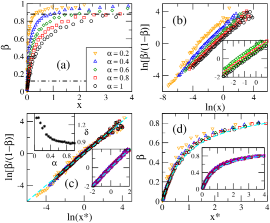
Figure 1: (a) Scaled localization length of eigenfunctions $\beta$ as a function of $x=b_{\mbox{\tiny eff}}^{2}/N$, $b_{\mbox{\tiny eff}}=\alpha b$, for the non-Hermitian diluted banded random matrix ensemble characterized by the sparsity $\alpha$. Several combinations of $(b,N)$ are used. Horizontal dot-dashed lines at $\beta\approx 0.12$ and 0.88 are shown as a reference, see the text. (b) Logarithm of $\beta/(1-\beta)$ as a function of $\ln(x)$. Inset: Enlargement in the range $\ln[\beta/(1-\beta)]=[-2,2]$ including data for $\alpha=0.6$, 0.8, and 1. Green-dashed lines are fittings of the data with Eq. (12). (c) Logarithm of $\beta/(1-\beta)$ as a function of $\ln(x^{*})$ [see Eq. (13)]. Upper inset: Power $\delta$, from the fittings of the curves $\ln[\beta/(1-\beta)]$ vs. $\ln(x)$ in the range $\ln[\beta/(1-\beta)]=[-2,2]$ with Eq. (12), as a function of $\alpha$. Lower Inset: Enlargement in the range $\ln[\beta/(1-\beta)]=[-2,2]$ including curves for $\alpha\in[0.5,1]$ in steps of $0.05$. Cyan-dashed lines in main panel and lower inset are Eq. (13). (d) $\beta$ as a function of $x^{*}$. Inset: Data for $\alpha\in[0.5,1]$ in steps of $0.05$. Cyan-dashed lines in main panel and inset are Eq. (14).

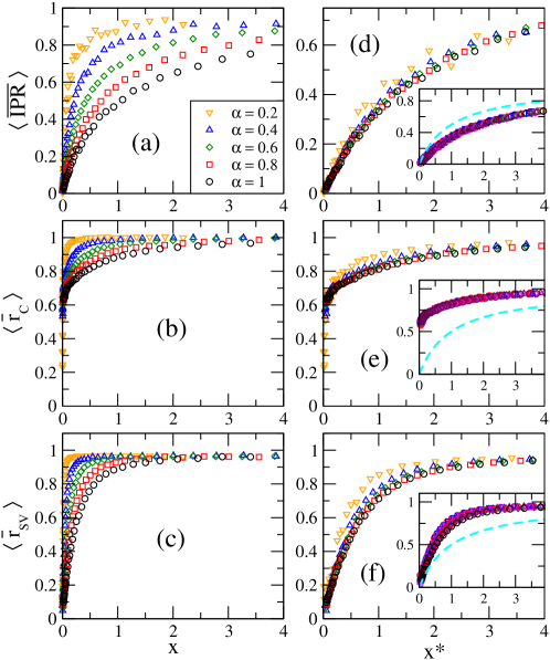
Figure 2: (a) $\left\langle\overline{\mbox{IPR}}\right\rangle$, (b) $\left\langle\overline{r}_{\mathbb{C}}\right\rangle$ and (c) $\left\langle\overline{r}_{\mbox{\tiny SV}}\right\rangle$ as a function of $x$ for the non-Hermitian diluted banded random matrix ensemble characterized by the sparsity $\alpha$. (d) $\left\langle\overline{\mbox{IPR}}\right\rangle$, (e) $\left\langle\overline{r}_{\mathbb{C}}\right\rangle$ and (f) $\left\langle\overline{r}_{\mbox{\tiny SV}}\right\rangle$ as a function of $x^{*}$. Insets in (d-f): Data for $\alpha\in[0.5,1]$ in steps of $0.05$. Dashed lines are Eq. (14).

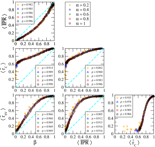
Figure 3: Scatter plots between $\beta$, $\left\langle\overline{\mbox{IPR}}\right\rangle$, $\left\langle\overline{r}_{\mathbb{C}}\right\rangle$ and $\left\langle\overline{r}_{\mbox{\tiny SV}}\right\rangle$ for the non-Hermitian diluted banded random matrix ensemble. Pearson’s correlation coefficients $\rho$ are reported in the corresponding panels.

In Fig. 1(a) we plot $\beta$ as a function of $x=b_{\mbox{\tiny eff}}^{2}/N$, with $b_{\mbox{\tiny eff}}=\alpha b$, for ensembles of matrices ${\bf nH}$ characterized by the sparsity $\alpha$. We observe that the curves of $\beta$ vs. $x$ show similar functional forms however clearly affected by the sparsity $\alpha$: That is, for a fixed $x$, the smaller the value of $\alpha$ the larger the value of $\beta$. This panorama is equivalent to that reported for the HdBRM ensemble in Ref. MFMR17b . Then, in Fig. 1(b) the logarithm of $\beta/(1-\beta)$ as a function of $\ln(x)$ is also presented. The quantity $\beta/(1-\beta)$ was useful in the study of the scaling properties of the BRM model CMI90 ; FM92 because $\beta/(1-\beta)\propto x$, which is equivalent to scaling (2), implies that a plot of $\ln[\beta/(1-\beta)]$ vs. $\ln(x)$ is a straight line with unit slope. Even though, this statement was valid for the BRM model in a wide range of parameters (i.e., for $\ln[\beta/(1-\beta)]<2$) it does not apply to the nHdBRM ensemble; see Fig. 1(b). In fact, from this figure we observe that plots of $\ln[\beta/(1-\beta)]$ vs. $\ln(x)$ are straight lines (in a wide range of $x$) with a slope that depends (slightly but detectably) on the sparsity $\alpha$. Consequently, we put to test the scaling law

$$\frac{\beta}{1-\beta}=\gamma x^{\delta},$$ (12)

which is equivalent to scaling (3), where both $\gamma$ and $\delta$ depend on $\alpha$.

Indeed, Eq. (12) describes well our data, mainly in the range $\ln[\beta/(1-\beta)]=[-2,2]$, as can be seen in the inset of Fig. 1(b) where we show the data for $\alpha=0.6$, 0.8 and 1 and include fittings with Eq. (12). We stress that the range $\ln[\beta/(1-\beta)]=[-2,2]$ corresponds to a reasonable large range of $\beta$ values, $\beta\approx[0.12,0.88]$, whose bounds are indicated with horizontal dot-dashed lines in Fig. 1(a). Also, we notice that the power $\delta$, obtained from the fittings of the data using Eq. (12), is quite close to unity for all the sparsity values we consider here; see the upper inset of Fig. 1(c).

Therefore, from the analysis of the data in Figs. 1(a,b), we can write down a universal scaling function for the scaled localization length $\beta$ of the nHdBRM model as

$$\frac{\beta}{1-\beta}=x^{*}\ ,\qquad x^{*}\equiv\gamma x^{\delta}.$$ (13)

To validate Eq. (13) in Fig. 1(c) we present again the data for $\ln[\beta/(1-\beta)]$ shown in Fig. 1(b) but now as a function of $\ln(x^{*})$. We do observe that curves for different values of $\alpha$ fall on top of Eq. (13) for a wide range of the variable $x^{*}$. Moreover, the collapse of the numerical data on top of Eq. (13) is excellent in the range $\ln[\beta/(1-\beta)]=[-2,2]$ for $\alpha\geq 0.5$, as shown in the lower inset of Fig. 1(c).

Finally, we rewrite Eq. (13) into the equivalent, but explicit, scaling function for $\beta$:

$$\beta=\frac{x^{*}}{1+x^{*}}.$$ (14)

In Fig. 1(d) we confirm the validity of Eq. (14). We would like to emphasize that the universal scaling given in Eq. (14) extends outsize the range $\beta\approx[0.12,0.88]$, for which Eq. (12) was shown to be valid, see the main panel of Fig. 1(d). Furthermore, the collapse of the numerical data on top of Eq. (14) is remarkably good for $\alpha\geq 0.5$, as shown in the inset of Fig. 1(d).

III.2 Other RMT measures

Now we complete the analysis of eigenfunction and spectral properties of the nHdBRM ensemble by computing the average inverse participation ratios $\left\langle\mbox{IPR}\right\rangle$ as well as the average ratios $\left\langle r_{\mathbb{C}}\right\rangle$ and $\left\langle r_{\mbox{\tiny SV}}\right\rangle$, see Eqs. (7,10,11). Moreover, we conveniently normalize these averages as follows:

$$\langle\overline{\mathrm{IPR}}\rangle=\frac{\langle\mathrm{IPR}\rangle-\mathrm{IPR}_{\mathrm{PE}}}{\mathrm{IPR}_{\mathrm{RGE}}-\mathrm{IPR}_{\mathrm{PE}}},$$ (15)

$$\langle\overline{r}_{\mathbb{C}}\rangle=\frac{\langle r_{\mathbb{C}}\rangle-r_{\mathbb{C}_{\mathrm{PE}}}}{r_{\mathbb{C}_{\mathrm{RGE}}}-r_{\mathbb{C}_{\mathrm{PE}}}}$$ (16)

and

$$\langle\overline{r}_{\mbox{\tiny SV}}\rangle=\frac{\langle r_{\mbox{\tiny SV}}\rangle-r_{{\mbox{\tiny SV}}_{\mathrm{PE}}}}{r_{{\mbox{\tiny SV}}_{\mathrm{RGE}}}-r_{{\mbox{\tiny SV}}_{\mathrm{PE}}}},$$ (17)

such that they all take values in the interval $[0,1]$, so they can be directly compared with $\beta$. The reference values used in Eqs. (15-17), corresponding to the PE and the RGE, are reported in Table 1.

Table 1: Reference average values for the Poisson ensemble and the real Ginibre ensemble, used in Eqs. (15-17), and the Gaussian orthogonal ensemble, to be used in the Appendix A.

	$\mathrm{IPR}$	$r_{\mathbb{C}}$	$r_{\mbox{\tiny SV}}$	$r_{\mathbb{R}}$
PE	1	0.5 PRRCM20	0.5 MA24	0.386 ABGR13
RGE	N/2.04 PM23	0.737 PRRCM20	0.569 MA24	–
GOE	N/3 OH07	0.569 PRRCM20	–	0.536 ABGR13

Then, in Figs. 2(a-c) we plot the normalized measures $\left\langle\overline{\mbox{IPR}}\right\rangle$, $\left\langle\overline{r}_{\mathbb{C}}\right\rangle$ and $\left\langle\overline{r}_{\mbox{\tiny SV}}\right\rangle$, respectively, as a function of $x$ for the nHdBRM ensemble characterized by the sparsity $\alpha$. The panorama shown in Figs. 2(a-c) for $\left\langle\overline{\mbox{IPR}}\right\rangle$, $\left\langle\overline{r}_{\mathbb{C}}\right\rangle$ and $\left\langle\overline{r}_{\mbox{\tiny SV}}\right\rangle$ is equivalent to that observed for $\beta$ in Fig. 1(a): The curves of $\left\langle\overline{X}\right\rangle$ vs. $x$ show similar functional forms however clearly affected by the sparsity $\alpha$. Here, $X$ represents IPR, $r_{\mathbb{C}}$ and $r_{\mbox{\tiny SV}}$. Also, for a fixed $x$, the smaller the value of $\alpha$ the larger the value of $\left\langle\overline{X}\right\rangle$. This observations allows us to surmise that the scaling parameter of $\beta$, $x^{*}$, may also serve as scaling parameter of $\left\langle\overline{X}\right\rangle$. To verify this assumption, in Figs. 2(d-f) we plot again $\left\langle\overline{\mbox{IPR}}\right\rangle$, $\left\langle\overline{r}_{\mathbb{C}}\right\rangle$ and $\left\langle\overline{r}_{\mbox{\tiny SV}}\right\rangle$, respectively, but now as a function of $x^{*}$. Indeed, since the curves $\left\langle\overline{X}\right\rangle$ vs. $x^{*}$ fall one on top of the other mainly for $\alpha\geq 0.5$, see the corresponding insets, we conclude that $x^{*}$ scales $\left\langle\overline{\mbox{IPR}}\right\rangle$, $\left\langle\overline{r}_{\mathbb{C}}\right\rangle$ and $\left\langle\overline{r}_{\mbox{\tiny SV}}\right\rangle$ as good as it scales $\beta$. From Fig. 2 we also observe that the curves $\left\langle\overline{r}_{\mathbb{C}}\right\rangle$ vs. $x^{*}$ and $\left\langle\overline{r}_{\mbox{\tiny SV}}\right\rangle$ vs. $x^{*}$ are above Eq. (14), which is included as dashed lines. This also means that the spectral properties of the nHdBRM model approach the RGE limit faster than the eigenfunction properties.

From Figs. 1 and 2 we can also see that all quantities ($\beta$, $\left\langle\overline{\mbox{IPR}}\right\rangle$, $\left\langle\overline{r}_{\mathbb{C}}\right\rangle$ and $\left\langle\overline{r}_{\mbox{\tiny SV}}\right\rangle$) appear to be highly correlated. Therefore, in Fig. 3 we present scatter plots between $\beta$, $\left\langle\overline{\mbox{IPR}}\right\rangle$, $\left\langle\overline{r}_{\mathbb{C}}\right\rangle$ and $\left\langle\overline{r}_{\mbox{\tiny SV}}\right\rangle$ for the nHdBRM ensemble for several values of $\alpha$, where the high correlation between them is evident. To quantify the correlation among these quantities, in the panels of Fig. 3 we report the corresponding Pearson’s correlation coefficient $\rho$, which turns out to be relatively large in all cases; i.e. $\rho>0.9$.

IV Discussion and conclusions

In this work, by using extensive numerical simulations, we demonstrate that the normalized localization length $\beta$ of the eigenfunctions of the diluted non-Hermitian banded random matrix (nHdBRM) ensemble scales with the parameter $x^{*}(N,b,\alpha)=\gamma(\alpha)[b_{\mbox{\tiny eff}}^{2}/N]^{\delta(\alpha)}$ as $\beta=x^{*}/(1+x^{*})$; see Fig. 1(d). Here, the effective bandwidth $b_{\mbox{\tiny eff}}\equiv\alpha b$ is the average number of non-zero elements per matrix row, $\alpha$ is the sparsity, $N$ is the matrix size, and $\gamma,\delta\sim 1$ are scaling parameters. Moreover, we also verified that $x^{*}$ works well as the scaling parameter of the average inverse participation ratios $\left\langle\overline{\mbox{IPR}}\right\rangle$ (another eigenfunction measure) as well as the spectral properties of the nHdBRM ensemble, characterized by the ratio between nearest- and next-to-nearest-neighbor (complex) eigenvalue distances $\left\langle\overline{r}_{\mathbb{C}}\right\rangle$ and the ratio between consecutive singular-value spacings $\left\langle\overline{r}_{\mbox{\tiny SV}}\right\rangle$; see Fig. 2(d-f). In addition, we also found that all these quantities ($\beta$, $\left\langle\overline{\mbox{IPR}}\right\rangle$, $\left\langle\overline{r}_{\mathbb{C}}\right\rangle$ and $\left\langle\overline{r}_{\mbox{\tiny SV}}\right\rangle$) are highly correlated; see Fig. 3.

In addition, for completeness, we also performed a detailed study of eigenfunction and spectral properties properties of the HdBRM ensemble MFMR17b ; see the Appendix A. Specifically, we report $\beta$, $\left\langle\overline{\mbox{IPR}}\right\rangle$, $\left\langle\overline{r}_{\mathbb{C}}\right\rangle$ and $\left\langle\overline{r}_{\mathbb{R}}\right\rangle$ where $r_{\mathbb{R}}$ is the ratio between consecutive eigenvalue spacings. Indeed, for the HdBRM ensemble we made similar conclusions as for the nHdBRM ensemble: That is, $\beta$ follows the scaling law of Eq. (14), see Fig. A1(d), and $x^{*}$ works well as the scaling parameter of $\left\langle\overline{\mbox{IPR}}\right\rangle$, $\left\langle\overline{r}_{\mathbb{C}}\right\rangle$ and $\left\langle\overline{r}_{\mathbb{R}}\right\rangle$, see Fig. A2(d-f). However, in contrast with the nHdBRM ensemble, for the HdBRM ensemble we found that $\left\langle\overline{\mbox{IPR}}\right\rangle$ follows the same scaling law as $\beta$ does, see Eq. (23) and Fig. A2(d).

Finally, we want to mention that both scalings (14) and (23) can be written in the “model independent” form (see e.g. FM92 ; CGIFM92 ):

$$\frac{1}{d(N,b,\alpha)}\approx\frac{1}{d(\infty,b,\alpha)}+\frac{1}{d(N,N,1)}.$$ (18)

Above, $d(N,b,\alpha)\equiv\exp[\left\langle S(N,b,\alpha)\right\rangle]$ and $d(N,N,1)=\exp[S_{\mbox{\tiny RGE}}(N)]$ (the reference entropy) for scaling (14), while $d(N,b,\alpha)\equiv\left\langle\mbox{IPR}(N,b,\alpha)\right\rangle$ and $d(N,N,1)=\mathrm{IPR}_{\mathrm{GOE}}$ for scaling (23).

Since diluted RM models can be used as null models for random networks (i.e. the adjacency matrices of complex networks are, in general, diluted random matrices), we believe that the nHdBRM ensemble may be used to model the adjacency matrices of certain types of directed random networks; that is, those having banded adjacency matrices. We hope our results may motivate a theoretical approach to the nHdBRM ensemble.

Appendix A Scaling properties of Hermitian diluted banded random matrices

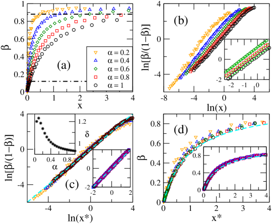
Figure A1: (a) Scaled localization length of eigenfunctions $\beta$ as a function of $x=b_{\mbox{\tiny eff}}^{2}/N$, $b_{\mbox{\tiny eff}}=\alpha b$, for the Hermitian diluted banded random matrix ensemble characterized by the sparsity $\alpha$. Several combinations of $(b,N)$ are used. Horizontal dot-dashed lines at $\beta\approx 0.12$ and 0.88 are shown as a reference. (b) Logarithm of $\beta/(1-\beta)$ as a function of $\ln(x)$. Inset: Enlargement in the range $\ln[\beta/(1-\beta)]=[-2,2]$ including data for $\alpha=0.6$, 0.8, and 1. Green-dashed lines are fittings of the data with Eq. (12). (c) Logarithm of $\beta/(1-\beta)$ as a function of $\ln(x^{*})$ [see Eq. (13)]. Upper inset: Power $\delta$, from the fittings of the curves $\ln[\beta/(1-\beta)]$ vs. $\ln(x)$ in the range $\ln[\beta/(1-\beta)]=[-2,2]$ with Eq. (12), as a function of $\alpha$. Lower Inset: Enlargement in the range $\ln[\beta/(1-\beta)]=[-2,2]$ including curves for $\alpha\in[0.5,1]$ in steps of $0.05$. Cyan-dashed lines in main panel and lower inset are Eq. (13). (d) $\beta$ as a function of $x^{*}$. Inset: Data for $\alpha\in[0.5,1]$ in steps of $0.05$. Cyan-dashed lines in main panel and inset are Eq. (14).

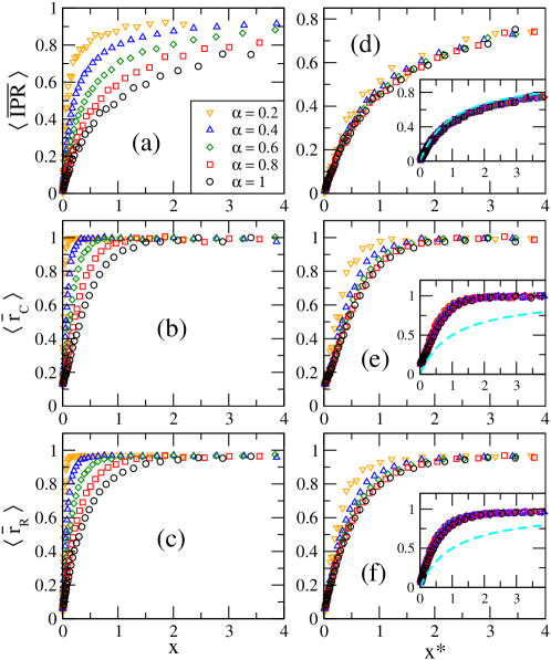
Figure A2: (a) $\left\langle\overline{\mbox{IPR}}\right\rangle$, (b) $\left\langle\overline{r}_{\mathbb{C}}\right\rangle$ and (c) $\left\langle\overline{r}_{\mathbb{R}}\right\rangle$ as a function of $x$ for the Hermitian diluted banded random matrix ensemble characterized by the sparsity $\alpha$. (d) $\left\langle\overline{\mbox{IPR}}\right\rangle$, (e) $\left\langle\overline{r}_{\mathbb{C}}\right\rangle$ and (f) $\left\langle\overline{r}_{\mathbb{R}}\right\rangle$ as a function of $x^{*}$. Insets in (d-f): Data for $\alpha\in[0.5,1]$ in steps of $0.05$. Dashed lines are Eq. (14).

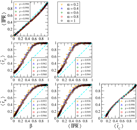
Figure A3: Scatter plots between $\beta$, $\left\langle\overline{\mbox{IPR}}\right\rangle$, $\left\langle\overline{r}_{\mathbb{C}}\right\rangle$ and $\left\langle\overline{r}_{\mathbb{R}}\right\rangle$ for the Hermitian diluted banded random matrix ensemble. Pearson’s correlation coefficients $\rho$ are reported in the corresponding panels.

Here, we report the scaling of eigenfunction and spectral properties of the matrices ${\bf H}$ belonging to the HdBRM ensemble. This is done for two main reasons: First, for comparison purposes; so we can contrast eigenfunction and spectral properties of the HdBRM and the nHdBRM ensembles. Second, for completeness; because in the study of the HdBRM ensemble presented in Ref. MFMR17b the spectral properties were only characterized by the repulsion parameter of Izrailev’s distribution of eigenvalue spacings and the $\mathrm{IPR}$ of the eigenfunctions was not reported.

Thus, as for the nHdBRM, we use exact numerical diagonalization to obtain the eigenfunctions $\Psi^{m}$ ($m=1\ldots N$) and eigenvalues of large ensembles of matrices ${\bf H}$ (which are members of the HdBRM ensemble) characterized by the parameters $N$, $b$, and $\alpha$. For each of the averages reported below we used at least $5\times 10^{5}$ data values.

In Fig. A1 we show the scaled localization length $\beta$ of eigenfunctions for the HdBRM ensemble. We compute $\beta$ as in Eq. (9) with

$$\ell_{N}=N\exp\left[-\left(S_{\mbox{\tiny GOE}}-\left\langle S\right\rangle\right)\right]\ ,$$

where $S_{\mbox{\tiny GOE}}\approx\ln(N/2.07)$. This because when $\alpha=1$ and $b=N$ the HdBRM becomes the GOE. Notice that, for comparison purposes, Fig. A1 is equivalent to Fig. 1 for the nHdBRM ensemble. We also note that all the information in Fig. A1 was reported in Figs. 1 and 2 of Ref. MFMR17b , however, for completeness, we decided to include it here. From Fig. A1 we can validate the following conclusion made in Ref. MFMR17b : The normalized localization length $\beta$ of the eigenfunctions of the HdBRM ensemble scales with the parameter $x^{*}(N,b,\alpha)=\gamma(\alpha)[(b\alpha)^{2}/N]^{\delta(\alpha)}$ as $\beta=x^{*}/(1+x^{*})$, see Fig. A1(d), where $\gamma,\delta\sim 1$.

Then, in Fig. A2 we report additional RMT measures to characterize eigenfunction and spectral properties of the HdBRM ensemble:

$$\langle\overline{\mathrm{IPR}}\rangle=\frac{\langle\mathrm{IPR}\rangle-\mathrm{IPR}_{\mathrm{PE}}}{\mathrm{IPR}_{\mathrm{GOE}}-\mathrm{IPR}_{\mathrm{PE}}},$$ (19)

$$\langle\overline{r}_{\mathbb{C}}\rangle=\frac{\langle r_{\mathbb{C}}\rangle-r_{\mathbb{C}_{\mathrm{PE}}}}{r_{\mathbb{C}_{\mathrm{GOE}}}-r_{\mathbb{C}_{\mathrm{PE}}}}$$ (20)

and

$$\langle\overline{r}_{\mathbb{R}}\rangle=\frac{\langle r_{\mathbb{R}}\rangle-r_{\mathbb{R}_{\mathrm{PE}}}}{r_{\mathbb{R}_{\mathrm{GOE}}}-r_{\mathbb{R}_{\mathrm{PE}}}},$$ (21)

The reference values used in Eqs. (19-21), corresponding to the GOE, are reported in Table 1. Note that Figs. A2(a,b,d,e) are equivalent to Figs. 2(a,b,d,e) for the nHdBRM ensemble. Also notice that here, for the HdBRM ensemble, we are not computing $\langle\overline{r}_{\mbox{\tiny SV}}\rangle$ since the spectrum of ${\bf H}$ is real and we do not need SVS. Instead, given the real and ordered spectrum of the Hermitian matrices ${\bf H}$, $\lambda_{1}>\lambda_{2}>\cdots>\lambda_{n}$, we compute the ratio $r_{\mathbb{R}}$ between consecutive level spacings, where the $i$–th ratio is given by ABGR13

$$r_{\mathbb{R}}^{i}=\frac{\mathrm{min}(\lambda_{i+1}-\lambda_{i},\lambda_{i}-\lambda_{i-1})}{\mathrm{max}(\lambda_{i+1}-\lambda_{i},\lambda_{i}-\lambda_{i-1})}.$$ (22)

From Fig. A2 we observe that $x^{*}$ works well as scaling parameter of $\left\langle\overline{\mbox{IPR}}\right\rangle$, $\left\langle\overline{r}_{\mathbb{C}}\right\rangle$ and $\left\langle\overline{r}_{\mathbb{R}}\right\rangle$ for the HdBRM ensemble, see Figs. A2(d-f). Perticularly for $\alpha\geq 0.5$, where all curves $\left\langle\overline{X}\right\rangle$ vs. $x^{*}$ fall one on top of the other; see the corresponding insets. Here, $X$ represents IPR, $r_{\mathbb{C}}$ and $r_{\mathbb{R}}$. Moreover, remarkably, $\left\langle\overline{\mbox{IPR}}\right\rangle$ approximately follows the same scaling law as $\beta$:

$$\left\langle\overline{\mbox{IPR}}\right\rangle\approx\frac{x^{*}}{1+x^{*}},$$ (23)

see the inset in Fig. A2(d).

Finally, in Fig. A3 we present the scatter plots between $\beta$, $\left\langle\overline{\mbox{IPR}}\right\rangle$, $\left\langle\overline{r}_{\mathbb{C}}\right\rangle$ and $\left\langle\overline{r}_{\mathbb{R}}\right\rangle$ for the HdBRM ensemble. We also include the Pearson’s correlation coefficients $\rho$ in the corresponding panels. Remarkably, we observe better correlations between eigenfunction measures (i.e. $\left\langle\overline{\mbox{IPR}}\right\rangle$ vs. $\beta$) and spectral measures (i.e. $\left\langle\overline{r}_{\mathbb{R}}\right\rangle$ vs. $\left\langle\overline{r}_{\mathbb{C}}\right\rangle$) for the HdBRM ensemble (where $\rho$ are very close to one) as compared with the nHdBRM ensemble.

References

- [1] The Oxford Handbook of Random Matrix Theory, G. Akemann, J. Baik, and P. Di Francesco (Eds.) (Oxford University Press, New York, 2011).
- [2] M. L. Metha, Random matrices (Elsevier, Amsterdam, 2004).
- [3] V. E. Kravtsov, I. M. Khaymovich, E. Cuevas, and M. Amini, A random matrix model with localization and ergodic transitions, New J. Phys. 17, 122002 (2015).
- [4] E. P. Wigner, Characteristic vectors of bordered matrices with infinite dimensions, Ann. Math. 62, 548 (1955).
- [5] E. P. Wigner, Ann. Math. 65, 203 (1957); SIAM Review 9, 1 (1967).
- [6] M. Wilkinson, M. Feingold, and D. M. Leitner, Localization and spectral statistics in a banded random matrix ensemble, J. Phys. A: Math. Gen. 24, 175 (1991).
- [7] M. Wilkinson, M. Feingold, and D. M. Leitner, Spectral statistics in semiclasical random-matrix ensembles, Phys. Rev. Lett. 66, 986 (1991).
- [8] M. Feingold, A. Gioletta, F. M. Izrailev, and L. Molinari, Two parameter scaling in the Wigner ensemble, Phys. Rev. Lett. 70, 2936 (1993).
- [9] G. Casati, B. V. Chirikov, I. Guarneri, and F. M. Izrailev, Band-random-matrix model for quantum localization in conservative systems, Phys. Rev. E 48, R1613 (1993).
- [10] G. Casati, B.V. Chirikov, I. Guarneri, and F. M. Izrailev, Quantum ergodicity and localization in conservative systems: the Wigner band random matrix model, Phys. Lett. A 223, 430 (1996).
- [11] M. Feingold, Localization in strongly chaotic systems, J. Phys. A: Math. Gen. 30, 3603 (1997).
- [12] W. Wang, Perturbative and nonperturbative parts of eigenstates and local spectral density of states: The Wigner-band random-matrix model, Phys. Rev. E 61, 952 (2000).
- [13] W. Wang, Approach to energy eigenvalues and eigenfunctions from nonperturbative regions of eigenfunctions, Phys. Rev. E 63, 036215 (2001).
- [14] A. D. Mirlin, Y. V. Fyodorov, F.-M. Dittes, J. Quezada, and T. H. Seligman, Transition from localized to extended eigenstates in the ensemble of power-law random banded matrices, Phys. Rev. E 54, 3221 (1996).
- [15] F. Evers and A. D. Mirlin, Anderson transitions, Rev. Mod. Phys. 80, 1355 (2008).
- [16] G. Casati, L. Molinari, and F. M. Izrailev, Scaling properties of band random matrices, Phys. Rev. Lett. 64, 1851 (1990).
- [17] S. N. Evangelou and E. N. Economou, Eigenvector statistics and multifractal scaling of band random matrices, Phys. Lett. A 151, 345 (1990).
- [18] Y. F. Fyodorov and A. D. Mirlin, Scaling properties of localization in random band matrices: A -model approach, Phys. Rev. Lett. 67, 2405 (1991).
- [19] L. V. Bogachev, S. A. Molchanov, L. A. Pastur, On the level density of random band matrices, Mathematical Notes 50:6, 1232 (1991).
- [20] S. A. Molchanov, L. A. Pastur, A. M. Khorunzhii, Limiting eigenvalue distribution for band random matrices, Theor. Math. Phys. 90:2, 108 (1992).
- [21] F. M. Izrailev, Scaling properties of spectra and eigenfunctions for quantum dynamical and disordered systems, Chaos Solitons Fractals 5, 1219 (1995).
- [22] Y. F. Fyodorov and A. D. Mirlin, Analytical derivation of the scaling law for the inverse participation ratio in quasi-one-dimensional disordered systems, Phys. Rev. Lett. 69, 1093 (1992).
- [23] A. D. Mirlin and Y. F. Fyodorov, The statistics of eigenvector components of random band matrices: Analytical results, J. Phys. A: Math. Gen. 26, L551 (1993).
- [24] Y. F. Fyodorov and A. D. Mirlin, Level-to-level fluctuations of the inverse participation ratio in finite quasi 1D disordered systems, Phys. Rev. Lett. 71, 412 (1993).
- [25] Y. F. Fyodorov and A. D. Mirlin, Statistical properties of eigenfunctions of random quasi 1D one-particle Hamiltonians, Int. J. Mod. Phys. B 8, 3795 (1994).
- [26] G. Casati, F. M. Izrailev, and L. Molinari, Scaling properties of the eigenvalue spacing distribution for band random matrices, J. Phys. A: Math. Gen. 24, 4755 (1991).
- [27] T. Kottos, A. Politi, F. M. Izrailev, and S. Ruffo, Scaling properties of Lyapunov spectra for the band random matrix model, Phys. Rev. E 53, R5553 (1996).
- [28] G. Casati, I. Guarneri, and G. Maspero, Landauer and Thouless conductance: A band random matrix approach, J. Phys. I (France) 7, 729 (1997).
- [29] T. Kottos, A. Politi, and F. M. Izrailev, Finite-size corrections to Lyapunov spectra for band random matrices, J. Phys.: Condens. Matter 10, 5965 (1998).
- [30] T. Kottos, F. M. Izrailev, and A. Politi, Finite-length Lyapunov exponents and conductance for quasi-1D disordered solids, Physica D 131, 155 (1999).
- [31] P. Shukla, Eigenvalue correlations for banded matrices, Physica E 9, 548 (2001).
- [32] W. Wang, Localization in band random matrix models with and without increasing diagonal elements, Phys. Rev. E 65, 066207 (2002).
- [33] K. K. Mon and J. B. French, Statistical properties of many-particle spectra, Ann. Phys. (N.Y.) 95, 90 (1975).
- [34] L. Benet and H. A. Weidenmüller, Review of the -body embedded ensembles of Gaussian random matrices, J. Phys. A: Math. Gen. 36, 3569 (2003).
- [35] V. K. B. Kota, Embedded random matrix ensembles in quantum physics, Lecture Notes in Physics 884 (Springer, London, 2014).
- [36] D. Cohen and T. Kottos, Parametric dependent Hamiltonians, wave functions, random matrix theory, and quantal-classical correspondence, Phys. Rev. E 63, 036203 (2001).
- [37] D. Cohen and E. J. Heller, Unification of perturbation theory, random matrix theory, and semiclassical considerations in the study of parametrically dependent eigenstates, Phys. Rev. Lett. 84, 2841 (2000).
- [38] D. L. Shepelyansky, Coherent propagation of two interacting particles in a random potential, Phys. Rev. Lett. 73, 2607 (1994).
- [39] Y. V. Fyodorov and A. D. Mirlin, Statistical properties of random banded matrices with strongly fluctuating diagonal elements, Phys. Rev. B 52, R11580 (1995).
- [40] Y. V. Fyodorov and A. D. Mirlin, Analytical results for random band matrices with preferential basis, Europhys. Lett., 32, 385 (1995).
- [41] P. G. Silvestrov, Summing graphs for random band matrices, Phys. Rev. E 55, 6419 (1997).
- [42] M. Disertori, H. Pinson, and T. Spencer, Density of states for random band matrices, Commun. Math. Phys. 232, 83 (2002).
- [43] A. Khorunzhy and W. Kirsch, On asymptotic expansions and scales of spectral universality in band random matrix ensembles, Commun. Math. Phys. 231, 223 (2002).
- [44] J. Schenker, Eigenvector localization for random band matrices with power law band width, Commun. Math. Phys. 290, 1065 (2009).
- [45] S. Sodin, The spectral edge of some random band matrices, Annals of Math. 172, 2223 (2010).
- [46] T. Prosen and M. Robnik, Energy level statistics and localization in sparsed banded random matrix ensemble, J. Phys. A: Math. Gen. 26, 1105 (1993).
- [47] Y. V. Fyodorov, O. A. Chubykalo, F. M Izrailev, and G. Casati, Wigner random banded matrices with sparse structure: Local spectral density of states, Phys. Rev. Lett. 76, 1603 (1996).
- [48] X. Cao, A. Rosso, J.-P. Bouchaud, P. LeDoussal, Genuine localisation transition in a long-range hopping model, Phys. Rev. E 95, 062118 (2017).
- [49] J. A. Mendez-Bermudez, F. A. Rodrigues, and D. A. Vega-Oliveros, Multifractality in random networks with long-range spatial correlations. to be submitted.
- [50] J. A. Mendez-Bermudez, G. Ferraz-de-Arruda, F. A. Rodrigues, and Y. Moreno, Scaling properties of multilayer random networks, Phys. Rev. E 96, 012307 (2017).
- [51] X. Cao, Disordered statistical physics in low dimensions. Extremes, glass transition, and localization, preprint arXiv:1705.06896 (2017).
- [52] G. J. Rodgers and A. J. Bray, Density of states of a sparse random matrix, Phys. Rev. B 37, 3557 (1988).
- [53] Y. V. Fyodorov and A D Mirlin, On the density of states of sparse random matrices, J. Phys. A: Math. Gen. 24, 2219 (1991).
- [54] Y. F. Fyodorov and A. D. Mirlin, Localization in ensemble of sparse random matrices, Phys. Rev. Lett. 67, 2049 (1991).
- [55] A. D. Mirlin and Y. V. Fyodorov, Universality of level correlation function of sparse random matrices, J. Phys. A: Math. Gen. 24, 2273 (1991).
- [56] S. N. Evangelou and E. N. Economou, Spectral density singularities, level statistics, and localization in a sparse random matrix ensemble, Phys. Rev. Lett. 68, 361 (1992).
- [57] S. N. Evangelou, A numerical study of sparse random matrices, J. Stat. Phys. 69, 361 (1992).
- [58] A. D. Jackson, C. Mejia-Monasterio, T. Rupp, M. Saltzer, and T. Wilke, Spectral ergodicity and normal modes in ensembles of sparse matrices, Nucl. Phys. A 687, 405 (2001).
- [59] O. Khorunzhy, M. Shcherbina, and V. Vengerovsky, Eigenvalue distribution of large weighted random graphs, J. Math. Phys. 45, 1648 (2004).
- [60] R. Kühn, Spectra of sparse random matrices, J. Phys. A: Math. Theor. 41, 295002 (2008).
- [61] S. Sodin, The Tracy-Widom law for some sparse random matrices, J. Stat. Phys. 136, 834 (2009).
- [62] G. Semerjian and L. F. Cugliandolo, Sparse random matrices: the eigenvalue spectrum revisited, J. Phys. A: Math. Gen. 35, 4837 (2002).
- [63] L. Erdös, A. Knowles, H.-T. Yau, and J. Yin, Spectral statistics of Erdös-Rényi graphs I: Local semicircle law, Ann. Probab. 41, 2279 (2013).
- [64] L. Erdös, A. Knowles, H.-T. Yau, and J. Yin, Spectral statistics of Erdös-Rényi graphs II: Eigenvalue spacing and the extreme eigenvalues, Commun. Math. Phys. 314, 587 (2012).
- [65] J. A. Mendez-Bermudez, A. Alcazar-Lopez, A. J. Martinez-Mendoza, F. A. Rodrigues, and T. K. DM. Peron, Universality in the spectral and eigenfunction properties of random networks, Phys. Rev. E 91, 032122 (2015).
- [66] J. A. Mendez-Bermudez, G. Ferraz-de-Arruda, F. A. Rodrigues, and Y. Moreno, Diluted banded random matrices: Scaling behavior of eigenfunction and spectral properties, J. Phys. A: Math. Theor. 50, 495205 (2017).
- [67] J. Ginibre, Statistical ensembles of complex, quaternion, and real matrices, J. Math. Phys. 6, 440 (1965).
- [68] C. M. Bender, Making sense of non-Hermitian Hamiltonians, Reports on Progress in Physics 70, 947–1018 (2007).
- [69] N. Moiseyev, Non-Hermitian Quantum Mechanics (Cambridge University Press, Cambridge, 2011)
- [70] Parity-Time symmetry in optics and photonics, D. N. Christodoulides, R. El-Ganainy, U. Peschel, and S. Rotter (editors) Focus issue, New J. Phys. (2016).
- [71] R. El-Ganainy, K. G. Makris, M. Khajavikhan, Z. H. Musslimani, S. Rotter and D. N. Christodoulides. Non-Hermitian physics and PT-symmetry, Nature Physics 14, 11 (2018).
- [72] J. F. Carpraux, J. Erhel, and M. Sadkane, Spectral portrait for non-hermitian large sparse matrices, Computing 53, 301–310 (1994).
- [73] T. Rogers and I. Perez-Castillo, Cavity approach to the spectral density of non-Hermitian sparse matrices, Phys. Rev. E 79, 012101 (2009).
- [74] F. L. Metz, I. Neri, and T. Rogers, Spectral theory of sparse non-Hermitian random matrices, J. Phys. A: Math. Theor. 52, 434003 (2019).
- [75] A. Basak and M. Rudelson, The circular law for sparse non-Hermitian matrices Ann. Probab. 47, 2359–2416 (2019).
- [76] I. Neri and F. L. Metz, Spectra of sparse non-Hermitian random matrices: An analytical solution, Phys. Rev. Lett. 109, 030602 (2012).
- [77] R. Aguilar-Sanchez, J. A. Mendez-Bermudez, F. A. Rodrigues, and J. M. Sigarreta-Almira, Topological versus spectral properties of random geometric graphs, Phys. Rev. E 102, 042306 (2020).
- [78] T. Peron, B. M. F. de Resende, F. A. Rodrigues, L. da F. Costa, and J. A. Mendez-Bermudez, Spacing ratio characterization of the spectra of directed random networks, Phys. Rev. E 102, 062305 (2020).
- [79] K. Peralta-Martinez and J. A. Mendez-Bermudez, Directed random geometric graphs: structural and spectral properties, J. Phys. Complex. 4, 015002 (2023).
- [80] Topological and spectral properties of random digraphs, C. T. Martinez-Martinez, J. A. Mendez-Bermudez, and J. M. Sigarreta, preprint arXiv:2311.07854.
- [81] J. A. Mendez-Bermudez and R. Aguilar-Sanchez, Singular-value statistics of directed random graphs, preprint arXiv:2404.18259.
- [82] G. Dubach and Y. Peled, On words of non-Hermitian random matrices, Ann. Probab. 49, 1886–1916 (2021).
- [83] I. Jana, CLT for non-Hermitian random band matrices with variance profiles, J. Stat. Phys. 187, 13 (2022).
- [84] G. Casati, I. Guarneri, F. M. Izrailev, and R. Scharf, Scaling behavior of localization in quantum chaos, Phys. Rev. Lett. 64, 5 (1990).
- [85] F. M. Izrailev, Simple models of quantum chaos: Spectrum and eigenfunctions, Phys. Rep. 196, 299 (1990).
- [86] G. Casati, I. Guarneri, F. M. Izrailev, S. Fishman, and L. Molinari, Scaling of the information length in 1D tight-binding models, J. Phys.: Condens. Matter 4, 149 (1992).
- [87] C. E. Shannon, Bell Syst. Tech. J 27, 379–423 (1948).
- [88] V. Oganesyan and D. A. Huse, Phys. Rev. B 75, 155111 (2007).
- [89] L. Sa, P. Ribeiro, and T. Prosen, Phys. Rev. X 10, 021019 (2020).
- [90] K. Kawabata, Z. Xiao, T. Ohtsuki, and R. Shindou, Singular-value statistics of non-Hermitian random matrices and open quantum systems, PRX Quantum 4, 040312 (2023).
- [91] Y. Y. Atas, E. Bogomolny, O. Giraud, G. Roux, Phys. Rev. Lett. 110, 084101 (2013).