Effects of a Vanishing Noise on Elementary Cellular Automata Phase-Space Structure

Abstract

We investigate elementary cellular automata (ECA) from the point of view of (discrete) dynamical systems. By studying small lattice sizes, we obtain the complete phase space of all minimal ECA, and, starting from a maximal entropy distribution (all configurations equiprobable), we show how the dynamics affects this distribution. We then investigate how a vanishing noise alters this phase space, connecting attractors and modifying the asymptotic probability distribution. What is interesting is that this modification not always goes in the sense of decreasing the entropy.
keywords: Elementary cellular automata, discrete dynamical systems, attractors, noise-induced transitions

1 Introduction

Cellular Automata (CA) are interesting systems, see the series of proceedings of this conference to get a wide scenario of this subject [1, 2, 3, 4, 5, 6, 7, 8, 9, 10, 11].

Deterministic Cellular Automata have been introduced as discrete dynamical systems by S. Wolfram [12]. We refer here to the well-known Wolfram’s numbering of Elementary Cellular Automata (ECA) rules, which are defined more precisely in Section 2.

Let us consider the space of all possible configurations of a finite lattice, with periodic boundary conditions, and denote it the phase-space and that will be studied in more details in Section 4. The dynamics connects configurations, originating trajectories. Since it is deterministic, we can have joining trajectories, but not separation. For finite lattices, trajectories, after a transient, always end into a cycle or a fixed point (which is a cycle with period equal to one), that constitutes the only attractors. Therefore, the phase-space is partitioned into basins of attractors.

Another way of looking at the dynamics properties of CA is that of measuring the stability of a trajectory with respect to some perturbation or noise, by observing the spreading of a damage [13] or defining indicators like Lyapunov exponents or similar ones [14, 15, 16].

CA rules can be classified according on the pattern they generate, which roughly corresponds to the kind and distribution of attractors and basins [12, 17].

In this paper we study Elementary CA (ECA), i.e., one dimensional, uniform, Boolean CA with three-sites interactions as (extended) dynamical systems, and we investigate the structure of their phase space.

In Section 2 we give some definition, then we present the phase space of ECA in Section 3 and the stability of their attractors in Section 4. In the following Section 5 we show how attractors are connected by a vanishing noise, and how the phase-space entropy if affected by noise and in Section 7 we furnish some algorithms to enumerate all attractors in small systems. Conclusions are drawn in the last section.

Table 1: Look-up table of some CA rules. Here $x,y,z$ stands for $s_{i-1},s_{i},s_{i+1}$.

x,y,z	R 1	R 164	R 232	R 11	R 30	R 150	R 204	R 110
0,0,0	1	0	0	1	0	0	0	0
0,0,1	0	0	0	1	1	1	0	1
0,1,0	0	1	0	0	1	1	1	1
0,1,1	0	0	1	1	1	0	1	1
1,0,0	0	0	0	0	1	1	0	0
1,0,1	0	1	1	0	0	0	0	1
1,1,0	0	0	1	0	0	0	1	1
1,1,1	0	1	1	0	0	1	1	0

2 Definitions

Cellular automata are completely discrete dynamical or statistical systems, defined on a lattice of cells, which can take a finite number of states. The evolution of the state of the cells is given by a function of their neighborhood, i.e., of the state of the cells connected with an incoming link to the cell itself.

In order to be more specific, let us define a network though an adjacency matrix $a$, where $a_{ij}=1$ if cell $i$ is connected (takes information) from cell $j$ and zero otherwise. In general, regular lattices with periodic boundary conditions are used, for which the adjacency matrix is shift-invariant (circulant). In particular, for Elementary Cellular Automata (ECA), a cell is connected to the cell itself and its two nearest neighbors, i.e., the matrix $a$ is tri-diagonal.

Let us denote by $s_{i}(t)$ the state of cell $i$ at time $t$. In order to be more concise, the index $t$ will be considered implicit, and we shall write $s_{i}^{\prime}\equiv s_{i}(t+1)$. Similarly, $v_{i}\equiv v_{i}(t)=\{s_{j}:a_{ij}=1\}$. ECA are Boolean Cellular Automata, i.e., $s_{i}=0,1$.

We denote by $v_{i}$ the state of its neighborhood, i.e., the states of cells $j$ such that $a_{ij}=1$. The in-grade $g_{i}$ of a cell, i.e., the size of its neighborhood, is defined as $g_{i}=\sum_{j}a_{ij}$, and for ECA it is 3.

Rule 1	Rule 164	Rule 232	Rule 11
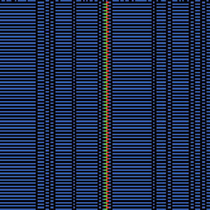
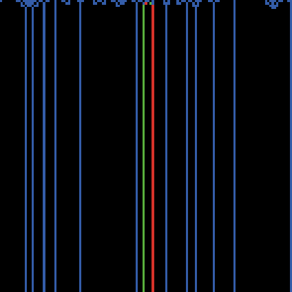
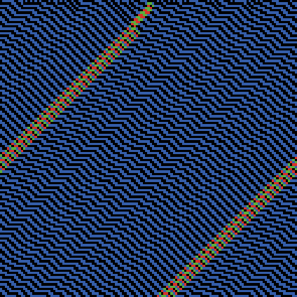
Rule 30	Rule 150	Rule 204	Rule 110

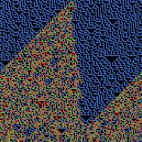
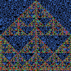
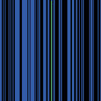
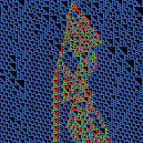
Figure 1: Time evolution of some rule starting from a random initial configuration ($s_{i}(t)$) and the evolution of an initial single defect ($S_{i}(t)$). Time runs from top to down. Color code: black: $s_{i}(t)=S_{i}(t)=0$; blue: $s_{i}(t)=1$, $S_{i}(t)=0$; blue: $s_{i}(t)=1$, $S_{i}(t)=0$; green: $s_{i}(t)=S_{i}(t)=1$; red: $s_{i}(t)=0$, $S_{i}(t)=1$;

The state of the neighborhood of a cell $i$, $v_{i}=\{s_{i-1},s_{i},s_{i+1}\}$, can also be read as a base-two number $v_{i}=4s_{i+1}+2s_{i}+s_{i-1}$; $0\leq v_{i}\leq 7$.

The evolution of the state of a cell is given by a function of the neighborhood $f(v)$, which is applied in parallel to all cells, $s_{i}^{\prime}=f(v_{i})$.

Since the neighborhood $v$ can take only a finite number of values, the function $f$ can be seen as a look-up table. Therefore, there are $2^{8}=256$ possible Boolean functions of three inputs, and each function is specified by listing the 8 values corresponding to $v=0,\dots,7$.

Reading again these lists of values as a base-2 numbers, $\{f(1,1,1),f(110),\dots$ $,f(0,0,0)\}$ we get the Wolfram notation for ECA, as illustrated for some rules in Table 1.

The time evolution of these rules is reported in Fig. 1. Rule 1, 164, 232 and 11 are typical class-2 rule,

The behavior of rules 22, 30 and 150 are similar, however rule 30 is not symmetric. Rule 204 is the identity. Rules 22, 150 and 232 are totalistic, since they depend on the sum of cell values in neighborhood (i.e., they are completely symmetric in their arguments). Rule 232 is the majority rule.

By exploiting left-right and 0-1 symmetry, we can reduce the number of independent rules to 88, called the “minimal” rules. These are rules 0, 1, 2, 3, 4, 5, 6, 7, 8, 9, 10, 11, 12, 13, 14, 15, 18, 19, 22, 23, 24, 25, 26, 27, 28, 29, 30, 32, 33, 34, 35, 36, 37, 38, 40, 41, 42, 43, 44, 45, 46, 50, 51, 54, 56, 57, 58, 60, 62, 72, 73, 74, 76, 77, 78, 90, 94, 104, 105, 106, 108, 110, 122, 126, 128, 130, 132, 134, 136, 138, 140, 142, 146, 150, 152, 154, 156, 160, 162, 164, 168, 170, 172, 178, 184, 200, 204, 232.

3 Dynamical properties of ECA

It is possible to define the Boolean derivative of a Boolean function [18, 19], which is similar to the usual definition: it takes value one if the change of a variable makes the function change, and zero otherwise.

Linear rule are those for which all derivatives are constant, i.e., variables appear only alone, possibly with a constant. Let us provide some examples.

$$f_{150}(x,y,z)=x\oplus y\oplus z;\qquad f_{204}(x,y,z)=y\\$$

are linear function, but $f_{204}$ is not peripherally linear, while

$$f_{0}=0;\qquad f_{22}(x,y,z)=x\oplus y\oplus z\oplus xyz$$

$$f_{30}(x,y,z)=x\oplus y\oplus z\oplus yz;\qquad f_{35}(x,y,z)=1\oplus x\oplus y\oplus xy\oplus xz\oplus xyz$$

$$f_{76}(x,y,z)=x\oplus xyz;\qquad f_{110}(x,y,z)=x\oplus y\oplus xy\oplus xyz$$

$$f_{178}(x,y,z)=x\oplus z\oplus xy\oplus xzvyz;\qquad f_{232}(x,y,z)=xy\oplus yz\oplus xz$$

are not.

Exploiting the Boolean derivatives, it is also possible to define the Jacobian $J$ for a given rule,

$$J_{ij}=\frac{\partial x^{\prime}_{i}}{\partial{s_{j}}}=\frac{\partial f(v_{i})}{\partial{s_{j}}}$$

which, for ECA, is a tri-diagonal circulant matrix (for periodic boundary conditions), that depends on the configuration $\{s_{i}(t)\}$, except for linear rules for which is constant.

By computing the maximum eigenvalue of the product of Jacobians over a trajectory it is possible to compute the maximum Lyapunov exponent of the trajectory [14], which corresponds to the spreading rate of a defect, in the limit of just one defect for each time step (i.e., taking replicas of the configuration at each time, and distributing the defects on each replica). In other words, this product gives all possible paths of a vanishing defects, i.e., supposing that only one defect can survive at each time step.

What is important for the present analysis is that even an unstable trajectory cannot be left, due to the Boolean nature of CA. For instance, the trajectory of rule 232 reported in Fig. 1 is unstable and shows a positive Lyapunov exponent, however for this rule any block of at least two cells with the same value gives origin to a permanent “stripe”. By adding a vanishing noise (i.e., at most one cell state flip per time step), the boundaries of a stripe can move. When meeting two boundaries fuse, making a strip disappear, while a new strip cannot appear (unless the nose is so high that two neighboring defects are created at the same time). Finally, all stripes coalesce (for periodic boundary conditions, if boundaries are fixed a frustration may be present). The stable configuration in the presence of a vanishing noise are those composed by all zeros and all ones, which have a negative (minus infinity) Lyapunov exponent.

This consideration illustrate the importance of examining the effects of a vanishing noise.

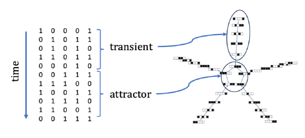
Figure 2: Transients and attractors for a basin.

4 ECA Attractor structure

If we consider the whole lattice,

$$\boldsymbol{s}(t)\equiv\{s_{i}(t),i=1,\dots,L\},$$

with appropriate (for instance periodic) boundary conditions, we can define a global function $\boldsymbol{F}$ so that

$$\boldsymbol{s}(t+1)=\boldsymbol{F}(\boldsymbol{s}(t)).$$

and this defines a discrete dynamical system.

For a Boolean lattice of $L$ sites, $\boldsymbol{s}$ can take $2^{L}$ possible values. Let us denote a trajectory $\gamma$ the ordered set of configurations given by the dynamics,

$$\gamma\equiv\gamma(\boldsymbol{s}(0))=\{\boldsymbol{s}(0),\boldsymbol{s}(1),\dots\}.$$

Since the evolution is deterministic and the number of states (on a finite lattice) is finite, a trajectory always ends in a cycle, possibly in a fixed point (which is cycle of length $1$). These limit cycles are the only attractors for finite CA. A cycle $\alpha$ is a trajectory $\alpha=\{\boldsymbol{s}(1),\boldsymbol{s}(2),\dots,\boldsymbol{s}(k)\}$ such that $\boldsymbol{s}(1)=\boldsymbol{F}(\boldsymbol{s}(k))$. The length of the cycle is indicated by $c(\alpha)$.

A generic trajectory is represented by a (possible empty) transient $\tau$ followed by a cycle $\alpha$: $\gamma(\boldsymbol{s}(0))=\{\tau(\boldsymbol{s}(0)),\alpha,\alpha,\dots\}$ where $\tau$ is the minimal one, i.e., it has no overlap with $\alpha$, see Fig. 2 for an illustration.

The basin $\beta(\alpha)$ of a cycle $\alpha$ is given by all configurations $\boldsymbol{s}$ such that $\gamma(\boldsymbol{s})=\{\tau(\boldsymbol{s}),\alpha\}$. The size of the basin is indicated by $b(\alpha)$. We can also arbitrarily number the cycles with an index $k=1,\dots,n$, so we can speak of length of cycle $k$, $c_{k}$, and size of its basin, $b_{k}$. Clearly, $\sum_{k}b_{k}=2^{L}$.

Rule 1	Rule 164	Rule 232	Rule 11
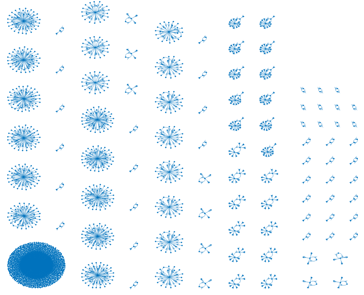
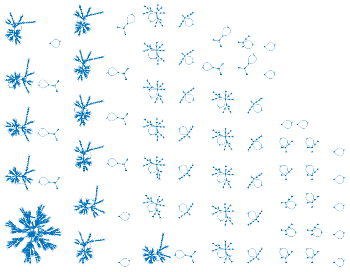
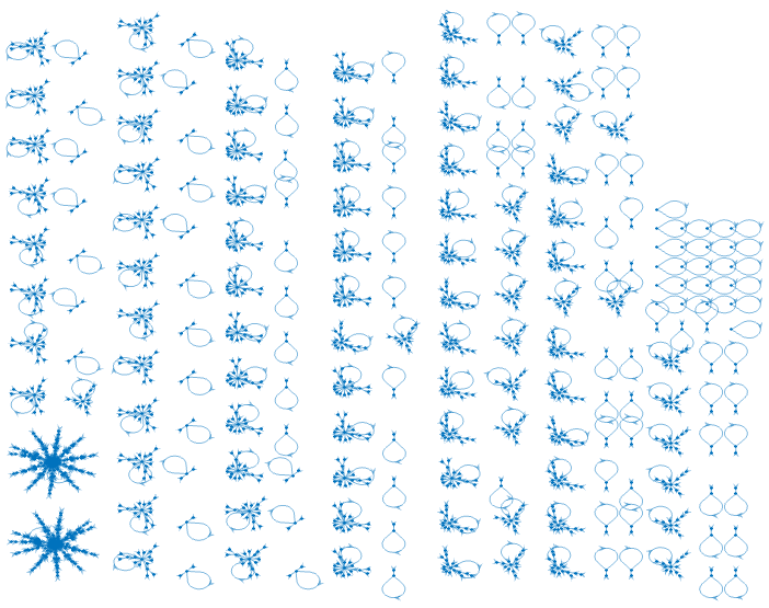
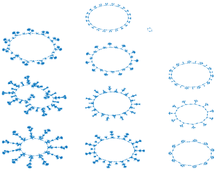
Rule 30	Rule 150	Rule 204	Rule 110

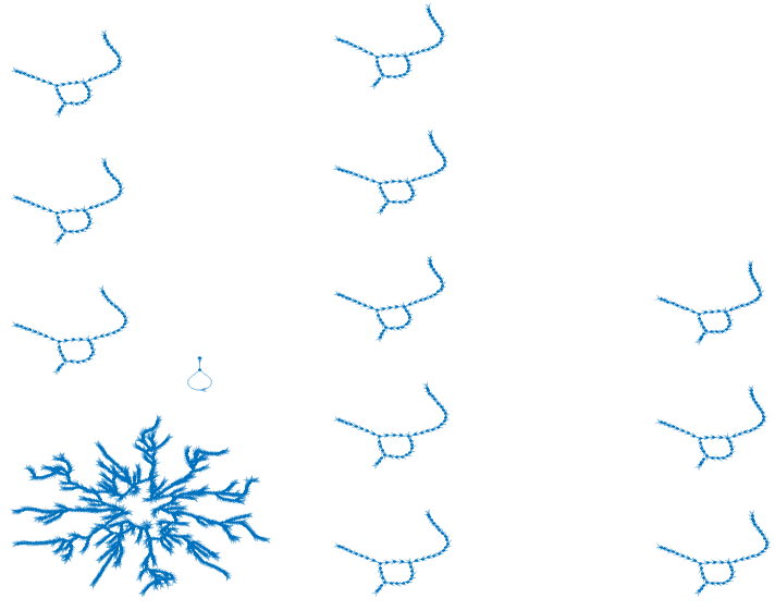
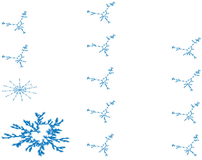
Figure 3: Attractors of rules shown in Fig. 1. Depending on the rule the dynamics shows different behaviors. For example, fixed point attractors (e.g., bottom left of rule 1), cycles with/without a basin of attraction (e.g., rule 30 and 150)

Another approach to the same problem is the following. Let us define the connection matrix $M_{\boldsymbol{s}^{\prime},\boldsymbol{s}}=M(\boldsymbol{s}^{\prime}|\boldsymbol{s})=1$ if $\boldsymbol{s}^{\prime}=\boldsymbol{F}(\boldsymbol{s})$ and zero otherwise (it is a $2^{L}\times 2^{L}$ matrix). $M$ clearly depends on the boundary conditions, that we assume are periodic. It is a (degenerate) Markov matrix, with $\sum_{\boldsymbol{s}}M_{\boldsymbol{s}^{\prime},\boldsymbol{s}}=1$ (actually, only one entry per columns of $M$ is one, all the rest is zero). If we start with a probability distribution of configurations $\boldsymbol{P}(\boldsymbol{s},0)$, we have

$$\boldsymbol{P}(\boldsymbol{s}^{\prime},t+1)=\sum_{\boldsymbol{S}}M(\boldsymbol{s}^{\prime}|\boldsymbol{s})\boldsymbol{P}(\boldsymbol{s},t).$$

Starting with a delta, $\boldsymbol{P}(\boldsymbol{s},0)=[\boldsymbol{s}=\boldsymbol{s}(0)]$, we get a sequence of deltas corresponding to the trajectory starting from $\boldsymbol{s}(0)$. After a transient time, the evolution enters an attractor cycle. The distributions corresponding to the states belonging to a cycle are eigenvectors of $M$.

We are interested in the maximally entropic starting state $\boldsymbol{P}(\boldsymbol{s},0)=2^{-L}$, for which the entropy is $S_{\mathrm{MAX}}=\log_{2}(L)$. If we iterate for a long time in many cases we finally get a distribution $\overline{\boldsymbol{P}}$ whose entries are zero for the configurations belonging to the transient part of cycle, and equal to $b_{k}/(2^{L}c_{k})$ for configurations belonging to a cycle, if all of them are the entry points in the limit cycle of transient trajectories with the same number of configurations. Since in cycle $k$ there are $c_{k}$ configurations we have

$$S(\overline{\boldsymbol{P}})=\frac{-1}{S_{\mathrm{MAX}}}\sum_{\boldsymbol{s}}\overline{\boldsymbol{P}}(\boldsymbol{s})\log_{2}(\overline{\boldsymbol{P}}(\boldsymbol{s}))=\frac{-1}{2^{L}\log_{2}(L)}\sum_{k=1}^{n}b_{i}\log_{2}\left(\frac{b_{i}}{c_{i}2^{L}}\right).$$

It may happen that the asymptotic distribution is oscillating, for instance Rule 1 maps all local configurations but $0,0,0$ to $0$, and the local configuration $0,0,0$ to $1$. So, starting from a homogeneous configuration, we have an alternation of deltas (corresponding to configurations $0,0,\dots$ and $1,1,\dots$).

The dynamics generally induces a production of information (reduction of entropy), which is related to the presence of transient states. One can have a visual representation of this contraction by looking at Fig. 3. One can see that in many cases there are transients, but this is not always true. For instance, Rule 204 (the identity) only has fixed points, while Rule 150 has many cycles and two fixed points ($\{0,0,\dots\}$ and $\{1,1,\dots\}$) with no transients.

The entropy $S$ is reported in Table 2 for all minimal rules and $L=17$. Let us illustrate some examples (see Fig. 1 and 3).

CA rule 0 (255) has a very simple structure: there is only one cycle, $\boldsymbol{s}=\{0,0,\dots\}$ ($\boldsymbol{s}=\{1,1,\dots\}$) whose basin includes all configurations ($K=1$), which fall into this cycle after one step: $b_{1}=2^{L}$. The final entropy is zero.

The phase space of the identity CA rule 204 is composed by $n=2^{L}$ fixed points (cycles of length $c_{k}=1$), each of them coincides with its own basin ($b_{k}=1$). The final relative entropy is one.

The phase space of the right shift CA 170 and of left-shift rule 240 is also composed by cycles which coincides with their basins, but they have different length: configuration $\{0,0,\dots\}$ is a fixed point, configuration $\{0,1,0,1,0,1,\dots\}$ and $\{1,0,1,0,1,0,\dots\}$ form of a cycle of length 2 for even $L$, but they have period $L$ if $L$ is odd, as all other non-symmetric configuration if $L$ is prime. In any case their asymptotic relative entropy is one.

The phase space of the majority CA 232 is composed by two fixed points $\boldsymbol{0}=\{0,0,\dots\}$ and $\boldsymbol{1}=\{1,1,\dots\}$ whose basin is composed by all configurations with isolated “other” values (i.e., of the type $\{0,0,\dots,1,1\dots,0,0\dots\}$, plus a number of other fixed points i.e., configuration with have at least two consecutive cells with the same value $\{0,0,\dots,1,1,\dots,0,0,\dots\}$. Rules 1 and 164 have similar phase spaces.

Finally, there are CA with very long cycles, which however depend on $L$. Since the evolution is parallel, any symmetry (reflection, inversion, translation) in the initial configuration cannot be forgotten, so one cannot have a cycle which includes symmetric and non-symmetric configurations. Therefore, the largest cycles are for $L$ prime, so that there no symmetric configurations are possible.

However, there are always two configurations, $\boldsymbol{s}=\{0,0,\dots\}$ and $\boldsymbol{s}=\{1,1,\dots\}$ which are translationally invariant, and which therefore cannot be part of a larger cycle.

The phase-space of the chaotic rule 150 is composed only by cycles, and again in this case the final relative entropy is one.

Not all chaotic CA have only cycles, for instance, for $L=11$, CA rule 30 has 13 attractors: configuration $\{0,0,\dots\}$ with a basin of 1, 11 cycles of length 17 and basin 45, and a long cycle of length 154 with a basin of 1551 configurations. Rule 110 has a similar phase space.

The computation of asymptotic probability distributions using the matrix $M$ (iterating or finding eigenvectors) is however computationally quite expensive, we shall give in Section 7 a more effective procedure.

Table 2: Number of attractors $n$, fraction of it with respect to the number of possible configurations $f=n\cdot 2^{-L}$, entropy induced by dynamics $S$ and entropy induced by a vanishing noise $S*$. Computations for all minimal rules R, lattice size $L=17$, $n_{\mathrm{MAX}}=131072$.

R	$n$	$S$	$S^{*}$	R	$n$	$S$	$S^{*}$	R	$n$	$S$	$S^{*}$	R	$n$	$S$	$S^{*}$
0	1	0	0	26	148	0.792	0.809	56	218	0.613	0.605	132	3572	0.6	0.624
1	1786	0.486	0.634	27	422	0.801	0.807	57	15	0.343	0.299	134	49	0.551	0.578
2	40	0.485	0.538	28	630	0.501	0.299	58	20	0.407	0.24	136	2	0	0
3	422	0.736	0.766	29	15777	0.863	0.857	60	260	0.941	0.941	138	837	0.791	0.764
4	3571	0.508	0.612	30	7	0.799	0.799	62	1186	0.611	0.607	140	3572	0.678	0.687
5	7158	0.736	0.766	32	1	0	0	72	664	0.323	0	142	317	0.572	0.393
6	48	0.577	0.607	33	1786	0.638	0.664	73	1361	0.71	0.681	146	121	0.587	0.586
7	42	0.502	0.059	34	211	0.678	0.687	74	101	0.642	0.656	150	8740	1	1
8	1	0	0	35	429	0.689	0.683	76	31553	0.85	0.85	152	41	0.515	0.535
9	24	0.45	0.451	36	664	0.323	0.445	77	3571	0.6	0.299	154	1688	1	1
10	211	0.678	0.687	37	349	0.531	0.517	78	120	0.377	0.24	156	631	0.502	0.299
11	108	0.594	0.299	38	234	0.731	0.738	90	4404	0.941	0.941	160	2	0	0
12	3571	0.678	0.687	40	8	0.001	0	94	1191	0.564	0.526	162	212	0.667	0.694
13	120	0.377	0.24	41	16	0.458	0.467	104	239	0.208	0	164	665	0.391	0.487
14	120	0.507	0.349	42	1857	0.839	0.862	105	4370	1	1	168	212	0.03	0
15	3856	1	1	43	316	0.572	0.393	106	214	0.699	0.701	170	7712	1	1
18	120	0.578	0.586	44	664	0.528	0.538	108	10966	0.776	0.764	172	704	0.5	0.538
19	1786	0.63	0.059	45	22	1	1	110	20	0.495	0.493	178	1787	0.6	0.299
22	52	0.44	0.46	46	40	0.544	0.533	122	120	0.588	0.588	184	422	0.572	0.567
23	1786	0.6	0.059	50	1786	0.6	0.299	126	120	0.578	0.588	200	14197	0.699	0
24	40	0.544	0.535	51	65536	1	1	128	2	0	0	204	131072	1	1
25	27	0.453	0.441	54	124	0.501	0.52	130	41	0.525	0.538	232	3572	0.6	0

5 Stability of attractors with respect to a vanishing noise

Another important issue is the effect of a vanishing noise. The idea is the following. I can perform a very small modification, i.e., flipping the value of some site but only occasionally and only at once. What are the effects of this vanishing perturbation?

Since the noise is vanishing, one can assume that the automata already reached an attractor. The smallest noise is the flipping of just a cell. This flipping causes a jump from a configuration to the perturbed one, which can belong to the basin of the same attractor or to that of another attractor. Thus, the effect of a vanishing noise is that of connecting the attractors.

Then, it is possible, exploiting the information obtained in Algorithm 1 to build a matrix $W_{ij}\equiv W(i|j)$ which counts, for all configurations belonging to cycle $j$, and for all possible perturbations, how many of them will belong to the basin of attractor $i$. Clearly, $\sum_{j}W_{ij}=L$.

Normalizing it over columns, one gets a Markov matrix $A_{ij}$ which gives the probability of going from attractor $j$ to attractor $i$ under the influence of a vanishing noise.

So, beyond the entropy reduction given by dynamics, we can have an entropy variation due to this noise. We shall denote the entropy on the probability distribution $\overline{\boldsymbol{Q}}$ obtained by iterating $\boldsymbol{Q}^{\prime}=A\boldsymbol{Q}$ with the symbol $S^{*}$.

What is interesting, is that this vanishing noise can act in different ways on CA rules. Results are reported on Table 2.

6 Noise effect

The effect of noise depends on the stability of attractor trajectories. This effect is clearly zero for “contracting” rules like rule 0, 8, etc. For these rules there is only one attractor, a stable fixed point with Jacobian equal to zero, so nothing happens and $S^{*}=S=0$.

The effect of noise is also zero for “flat” rules like the identity 204 or the shift 170. In these cases, the Jacobian is diagonal (eventually circularly shifted by one) and therefore the perturbation is simply maintained, so $S^{*}=S=S_{\mathrm{MAX}}$, irrespective of noise.

A similar result occurs for the linear rule 150. In this case the effect of noise propagates on all the lattice, but, since there is no preferred attractor, it has no influence on the probability distribution.

In general, the statistical properties of “chaotic” rules like 30, 110 are not affected by noise, except for rule 22 which shows a slight increase of entropy.

In many case there is an entropy reduction by noise. This is particularly evident for rule 232. In this case, most of attractors are composed by configuration made by clusters of zeros and ones of at least width 2. These configurations are stable with respect to single perturbations inside a cluster but are “connected” by perturbations at the boundary of a cluster.

For vanishing noise, these boundaries perform a self-annihilated random walk, so that the effect of the noise is to drive the system to the stable configurations 0 and 1.

This is also the case of rule 13 and 77, for which the asymptotic configuration is an alternation of zeros and ones, with occasionally clusters of double zeros which however can move and self-annihilate in the presence of noise. The same happens for instance to rule 58 for which a stable (translating) configuration is a repetition of $\{1,1,0,\}$, and the noise serves to remove the $\{1,0,1,0\}$ defects.

For a few rules, entropy increases by noise, but not for the trivial effect of introducing disturbances, since the measure is always performed on the distribution of attractors. Let us take as an example rule 1.

In this rule, the local pattern $\{0,0,0\}$ gives 1, all other patterns give zero. All isolated zeros in the initial configuration are removed, while isolated 1 maintains (every other step). So, the effect of noise is that of creating cluster of isolated ones in a greater number with respect to the random initialization process, and entropy increases.

A similar increase in entropy is observed for Rule 164. In this case,too, the effect of noise is that of connecting basins with few states (with low statistical weight starting from a random configuration) to configurations belonging to the largest basin.

global $A$;

$A(0:2^{L}-1)\leftarrow 0$;

$k\leftarrow 1$;

  /* attractor index */

$s_{0}\leftarrow 0$;

  /* first configuration */

while $s_{0}<2^{L}$ do

       $s\leftarrow s_{0}$;

        /* working configuration */

       while $A(s)=0$ do

             $A(s)\leftarrow-k$ /* negative indices denote transient configurations */ $s\leftarrow F(s)$;

              /* iteration */

            

       end while

      if  $A(s)=-k$  then /* entered the cycle */

             while $A(s)=-k$ do

                   $A(s)\leftarrow k$;

                    /* positive indices denote cycle */

                   $s\leftarrow F(s)$;

                  

             end while

            $k\leftarrow k+1$;

              /* increase the attractor number */

            

      else /* encountered another cycle */

             $m\leftarrow|A(s)|$;

              /* index of the other cycle */

             $s\leftarrow s_{0}$;

              /* restarting */

             $\mathbf{relabel}(s,m)$;

            

       end if

      $s_{0}\leftarrow s_{0}+1$;

        /* next configuration */

      

end while

Algorithm 1 Finding attractors and basins

global $A$;

relabel $(s,m)$

       while $|A(s)|\neq m$ do

             $A(s)\leftarrow-m$;

             $s\leftarrow F(s)$;

            

       end while

      

end

Algorithm 2 Relabeling transients

7 Numerical determination of attractors for small configurations

One can find all attractors and their characteristics for a small-size cellular automata, by enumerating all of them, following their evolution until entering a limit cycle, and numbering these cycles (see algorithm 1).

Let $L$ be the size of CA. There are $2^{L}$ possible configurations $\boldsymbol{s}$, which can be read as a base-two number $s$ from 0 to $2^{L}-1$. Let $A$ be an array of size $2^{L}$ set to zero. The idea is to label each configuration in a trajectory $\{s(0),s(1),\dots\}$ with the same index $-k$, until we find a configuration $S$ which is alredy marked (i.e., $A(S)\neq 0$. if $A(S)=-k$ then we proceed by inverting the sign of all configurations in the trajectory until we find a positive entry, i.e., we have ended the cycle. We then increment $k$.

If $|A(S)|\neq k$ if means that the trajectory belongs to the basin of an already encountered attractor, so we restart from $s(0)$ and we change all $k$ with $|A(S)|$. We do not increase $k$ after.

When there are no more configurations we have found all attractors and basins, and we can count the length of cycle $k$ (the number of entries $A(s)=-k$) and its size (the number of entries $|A(s)|=k$), for $k=1,\dots,n$.

8 Conclusions

We investigated elementary cellular automata as discrete dynamical systems. We obtained the complete phase-space (i.e. accessible states, attractors, basins of attraction) of all minimal ECA for small lattice sizes, and, starting from a maximal entropy distribution (i.e., all configurations equiprobable), we have shown how the dynamics affects this distribution, implying in general a reduction of entropy.

We then investigated how a vanishing noise alters the phase-space landscape, connecting attractors and modifying the asymptotic probability distribution over configurations.For chaotic rules and in general for those rules for which the dynamics does not reduce the entropy, noise has no effect on it.

In many of the other cases, the noise decreases the entropy, since it connects unstable limit cycles or fixed points to the basin of stable one.

In a few case, the opposite happens. This, is probably due to the instability of the limit cycle of the largest attractor. The connections between stability (Lyapunov exponents) and attractors, and the application of statistical techniques for dealing with larger lattices will be the subject of future work.

References

- [1] “Cellular Automata: 5th International Conference on Cellular Automata for Research and Industry, ACRI 2002 Geneva, Switzerland, October 9–11, 2002 Proceedings” In Lecture Notes in Computer Science Springer Berlin Heidelberg, 2002 DOI: 10.1007/3-540-45830-1
- [2] “Cellular Automata: 6th International Conference on Cellular Automata for Research and Industry, ACRI 2004, Amsterdam, The Netherlands, October 25-28, 2004. Proceedings” In Lecture Notes in Computer Science Springer Berlin Heidelberg, 2004 DOI: 10.1007/b102055
- [3] “Cellular Automata: 7th International Conference on Cellular Automata, for Research and Industry, ACRI 2006, Perpignan, France, September 20-23, 2006. Proceedings” In Lecture Notes in Computer Science Springer Berlin Heidelberg, 2006 DOI: 10.1007/11861201
- [4] “Cellular Automata: 8th International Conference on Cellular Aotomata for Reseach and Industry, ACRI 2008, Yokohama, Japan, September 23-26, 2008. Proceedings” In Lecture Notes in Computer Science Springer Berlin Heidelberg, 2008 DOI: 10.1007/978-3-540-79992-4
- [5] “Cellular Automata: 9th International Conference on Cellular Automata for Research and Industry, ACRI 2010, Ascoli Piceno, Italy, September 21-24, 2010. Proceedings” In Lecture Notes in Computer Science Springer Berlin Heidelberg, 2010 DOI: 10.1007/978-3-642-15979-4
- [6] “Cellular Automata: 10th International Conference on Cellular Automata for Research and Industry, ACRI 2012, Santorini Island, Greece, September 24-27, 2012. Proceedings” In Lecture Notes in Computer Science Springer Berlin Heidelberg, 2012 DOI: 10.1007/978-3-642-33350-7
- [7] “Cellular Automata: 11th International Conference on Cellular Automata for Research and Industry, ACRI 2014, Krakow, Poland, September 22-25, 2014. Proceedings” In Lecture Notes in Computer Science Springer International Publishing, 2014 DOI: 10.1007/978-3-319-11520-7
- [8] “Cellular Automata: 12th International Conference on Cellular Automata for Research and Industry, ACRI 2016, Fez, Morocco, September 5-8, 2016. Proceedings” In Lecture Notes in Computer Science Springer International Publishing, 2016 DOI: 10.1007/978-3-319-44365-2
- [9] “Cellular Automata: 13th International Conference on Cellular Automata for Research and Industry, ACRI 2018, Como, Italy, September 17–21, 2018, Proceedings” In Lecture Notes in Computer Science Springer International Publishing, 2018 DOI: 10.1007/978-3-319-99813-8
- [10] “Cellular Automata: 14th International Conference on Cellular Automata for Research and Industry, ACRI 2020, Lodz, Poland, December 2–4, 2020, Proceedings” In Lecture Notes in Computer Science Springer International Publishing, 2021 DOI: 10.1007/978-3-030-69480-7
- [11] “Cellular Automata: 15th International Conference on Cellular Automata for Research and Industry, ACRI 2022, Geneva, Switzerland, September 12–15, 2022, Proceedings” In Lecture Notes in Computer Science Springer International Publishing, 2022 DOI: 10.1007/978-3-031-14926-9
- [12] Stephen Wolfram “Statistical mechanics of cellular automata” In Reviews of modern physics 55.3 APS, 1983, pp. 601 DOI: 10.1103/revmodphys.55.601
- [13] D. Stauffer “Dynamics and Damage Spreading in Cooperative Systems: A Numerical Search for Universality” In Universalities in Condensed Matter Springer Berlin Heidelberg, 1988, pp. 246–249 DOI: 10.1007/978-3-642-51005-2_50
- [14] F. Bagnoli, R. Rechtman and S. Ruffo “Damage spreading and Lyapunov exponents in cellular automata” In Physics Letters A 172.1–2 Elsevier BV, 1992, pp. 34–38 DOI: 10.1016/0375-9601(92)90185-o
- [15] M.. Shereshevsky “Lyapunov exponents for one-dimensional cellular automata” In Journal of Nonlinear Science 2.1 Springer ScienceBusiness Media LLC, 1992, pp. 1–8 DOI: 10.1007/bf02429850
- [16] Jan Baetens and Janko Gravner “Introducing Lyapunov profiles of cellular automata” In Journal of Cellular Automata 13.3, 2018, pp. 267–286
- [17] Wentian Li and Norman Packard “The structure of the elementary cellular automata rule space” In Complex systems 4.3, 1990, pp. 281–297
- [18] Gérard Y. Vichniac “Boolean derivatives on cellular automata” In Physica D: Nonlinear Phenomena 45.1–3 Elsevier BV, 1990, pp. 63–74 DOI: 10.1016/0167-2789(90)90174-n
- [19] Franco Bagnoli “Boolean derivatives and computation of cellular automata” In International Journal of Modern Physics C 3.02 World Scientific, 1992, pp. 307–320 DOI: 10.1142/s0129183192000257