[3,4]\fnmEdward \surLinscott
1]\orgdivDepartment of Chemistry, \orgnameUniversity of Zurich, \orgaddress\postcode8057 \cityZurich, \countrySwitzerland
2]\orgdivTheory and Simulations of Materials (THEOS) and National Centre for Computational Design and Discovery of Novel Materials (MARVEL), \orgnameÉcole Polytechnique Fédérale de Lausanne, \orgaddress\postcode1015 \cityLausanne, \countrySwitzerland
3]\orgdivLaboratory for Materials Simulations (LMS), \orgnamePaul Scherrer Institute, \orgaddress\postcode5352 \cityVilligen, \countrySwitzerland
4]\orgdivNational Centre for Computational Design and Discovery of Novel Materials (MARVEL), \orgnamePaul Scherrer Institute, \orgaddress\postcode5352 \cityVilligen, \countrySwitzerland
Predicting electronic screening for fast Koopmans spectral functional calculations
Abstract
Koopmans spectral functionals represent a powerful extension of Kohn-Sham density-functional theory (DFT), enabling accurate predictions of spectral properties with state-of-the-art accuracy. The success of these functionals relies on capturing the effects of electronic screening through scalar, orbital-dependent parameters. These parameters have to be computed for every calculation, making Koopmans spectral functionals more expensive than their DFT counterparts. In this work, we present a machine-learning model that — with minimal training — can predict these screening parameters directly from orbital densities calculated at the DFT level. We show on two prototypical use cases that using the screening parameters predicted by this model, instead of those calculated from linear response, leads to orbital energies that differ by less than 20 meV on average. Since this approach dramatically reduces run-times with minimal loss of accuracy, it will enable the application of Koopmans spectral functionals to classes of problems that previously would have been prohibitively expensive, such as the prediction of temperature-dependent spectral properties.
1 Introduction
Predicting the spectral properties of materials from first principles can greatly assist the design of optical and electronic devices [1]. Among the various techniques one can employ, Koopmans spectral functionals are a promising technique due to their accuracy and comparably low computational cost [2, 3, 4, 5, 6, 7, 8, 9, 10, 11, 12]. These functionals are a beyond-DFT extension explicitly designed to predict spectral properties, and have shown success across a range of both isolated and periodic systems. For isolated systems, Koopmans functionals accurately predict the ionization potentials and electron affinities — and more generally, the orbital energies and photoemission spectra — of atoms [3], small molecules [5, 9, 13], organic photovoltaic compounds [14, 15], DNA nucleobases [16], and toy models [17]. The method has also been extended to predict optical (i.e. neutral) excitation energies in molecules [18]. For three-dimensional systems, Koopmans functionals have been shown to accurately predict the band structure and band alignment of prototypical semiconductors and insulators [8, 10, 11, 19], systems with large spin-orbit coupling [20], and a vacancy-ordered double perovskite [21], as well as the band gap of liquid water [22].
One of the crucial quantities involved in the definition of Koopmans functionals is the set of so-called screening parameters, denoted . These parameters account for the effect of electronic screening in the localized basis of the orbitals minimizing the functional. There is one screening parameter per orbital in the system, and each screening parameter can be computed fully from first-principle calculations using finite differences [3, 8] or with linear-response theory [9]. Obtaining reliable screening parameters is essential to the accuracy of Koopmans spectral functionals, while also being the main reason why these functionals are more expensive than their KS-DFT counterparts. The objective of this work is to replace the calculation of screening parameters with a machine-learning (ML) model, thereby drastically reducing the cost of Koopmans functional calculations, and making it possible to apply them more widely.
In the broader context of computational materials science and quantum chemistry, machine learning is being used to predict an ever-increasing range of quantum mechanical properties [23, 24], including electronic excitations [25, 26, 27]. In contrast to many of these approaches, the screening parameters studied in this work are intermediate quantities, not physical observables. In this regard, this work shares parallels with attempts to learn the parameter for DFT+ functionals [28, 29, 30, 31] and the dielectric screening when solving the Bethe-Salpeter equation [32] (albeit in the latter case the dielectric screening is a physical observable, but for the purposes of that work it was used as an ingredient for subsequent calculations of optical spectra). This work also differs from ML methods that seek to relate structural information directly to observable quantities on a practical level [33, 34, 35, 36, 37, 38, 39, 40, 41, 42], because in our case first-principles calculations will not be bypassed completely.
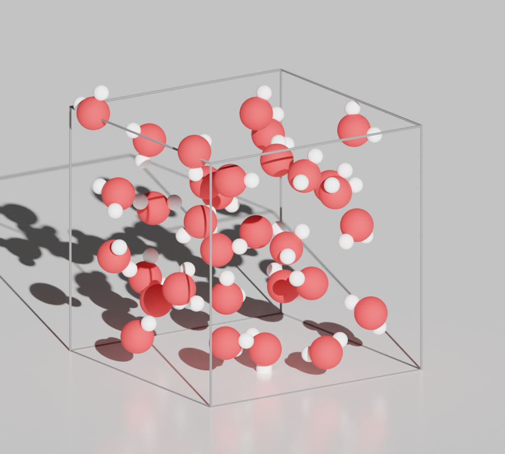
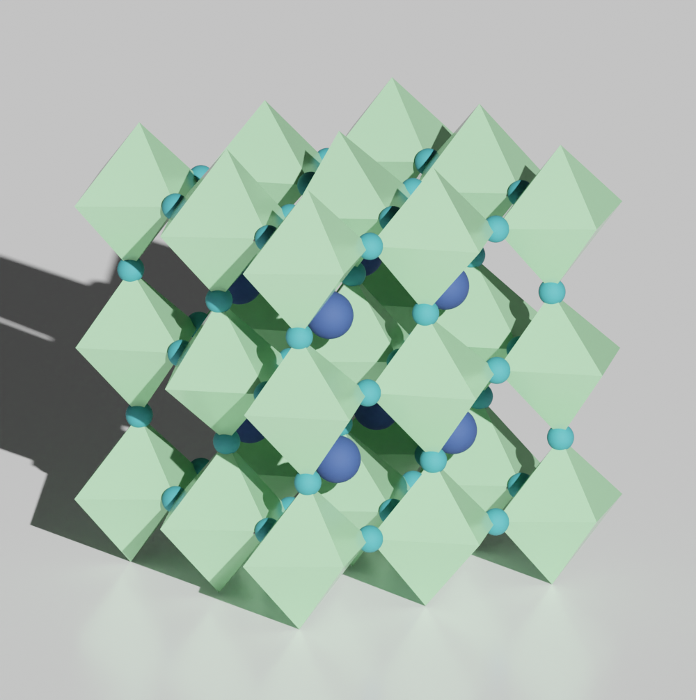
Specifically, we will present a simple machine learning framework that can be used to predict the screening parameters for a given chemical system (i.e., we do not develop a general model to predict the screening parameters for an arbitrary chemical system). The two use-cases we will study are liquid water and the halide perovskite \chCsSnI3 (fig. 1). In the case of liquid water, one might want to calculate spectral properties averaged along a molecular dynamics trajectory. In the case of the halide perovskite, one might want to calculate the temperature-renormalized band structure by performing calculations on an ensemble of structures with the atoms displaced in such a way to appropriately sample the ionic energy landscape [43, 44]. In both cases, these methods require Koopmans spectral functional calculations on many copies of the same chemical system, just with different atomic displacements. This process can be made much faster by training a machine learning model on a subset of these copies, and then using this model to predict the screening parameters for the remaining copies.
The contents of this paper are as follows: Section 2 introduces Koopmans functionals, focusing in particular on the screening parameters: why they are necessary, what their role is, and how they can be calculated ab initio. In Section 3 we then present a machine learning model designed to accelerate the computation of these screening parameters. In Section 4 we present the results of this model on two test systems: liquid water and the perovskite \chCsSnI3, and in Section 5 we discuss the results and draw our conclusions.
2 Koopmans spectral functionals and their screening parameters
Koopmans spectral functionals are a class of orbital-density dependent functionals that accurately predict spectral properties by imposing the condition that the quasi-particle energies of the functional must match the corresponding total energy difference when an electron is explicitly removed from/added to the system. This quasiparticle/total-energy-difference equivalence is trivially satisfied by the exact one-particle Green’s function (as can be seen by the spectral representation, with poles located at energies corresponding to particle addition/removal), but it is violated by standard Kohn-Sham density functionals and leads to, among other failures, semi-local DFT’s underestimation of the band gap. Given that the exact Green’s function describes one-particle excitations exactly, the idea behind Koopmans functionals is that enforcing this condition on DFT will improve its description of one-particle excitations.
An orbital energy, defined as , will be equal to the total energy difference of electron addition/removal if it is independent of that orbital’s occupation . (This follows because if — which is equal to by Janak’s theorem — is independent of , then the total energy difference [45].) Equivalently, the orbital energies will match the corresponding total energy differences if the total energy itself is piecewise-linear with respect to orbital occupations:
| (1) |
This condition is referred to as the “generalised piecewise linearity” (GPWL) condition. It is a sufficient but not a necessary condition to satisfy the more well-known “piecewise linearity” condition, which states that the exact total energy is piecewise-linear with respect to the total number of electrons in the system [46].
Koopmans functionals impose this GPWL condition on a (typically semi-local) DFT functional via tailored corrective terms as follows:
| (2) |
where are the orbital occupancies and the total electronic density of the -electron ground state, and denotes the electronic density of the ()-electron system with the orbital occupancies constrained to be equal to i.e. and correspond to charged excitations of the ground state where we fill/empty orbital . In the final line of eq. 2 we have introduced the shorthand for the Koopmans correction to orbital . By construction, this correction removes the non-linear dependence of the DFT energy on the occupation of orbital (the second line in eq. 2) and replaces it with a term that is explicitly linear in (the third line), with a slope that corresponds to the finite energy difference between integer occupations of orbital . We note that other choices are possible for the slope of this linear term, which give rise to different variants of Koopmans spectral functionals. In this paper, we will exclusively focus on this “Koopmans integral” (KI) variant.
While eq. 2 formally imposes the GPWL condition as desired, practically it cannot be used as a functional because we cannot construct the constrained densities without explicitly performing constrained DFT calculations. In order to convert eq. 2 into a tractable form, we instead evaluate these constrained densities in the frozen orbital approximation i.e. we neglect the dependence of the orbitals on the occupancy of orbital , obtaining
| (3) |
where are the orbitals of the unconstrained -electron ground state and we have introduced the shorthand for the normalized density of orbital and . These frozen densities — unlike their unfrozen counterparts — are straightforward to evaluate because they are constructed purely from quantities corresponding to the -electron ground state.
Evaluating the KI correction on frozen-orbital densities gives rise to the unscreened KI corrections . The orbital relaxation that is absent in these terms can be accounted for by appropriately screening the Koopmans corrections i.e.
| (4) |
where is some as-of-yet unknown scalar coefficient. The limit corresponds to an orbital that if its occupation changes, the rest of the electronic density does not respond. In contrast, the limit corresponds an orbital that if its occupation changes, the rest of the system will fully screen the change in the density. These parameters are the screening parameters that are the central topic of this work, and they will be discussed in more detail later.
Having introduced these screening parameters, we arrive at the final form of the KI functional:
| (5) |
where in the Koopmans correction only the Hartree-plus-exchange-correlation term appears because all the other terms in are linear in the orbital occupations and therefore cancel.
In contrast to standard DFT energy functionals, this energy functional is not only dependent on the total density but also on these individual orbital densities . Therefore one has to minimize the total energy functional with respect to the entire set of orbital densities to obtain the ground state energy, and not just with respect to the total density . (This is not so different to Kohn-Sham DFT, where one minimizes the functional with respect to a set of Kohn-Sham orbitals.)
The orbitals that minimize the Koopmans energy functional are called the variational orbitals. They are found to be localized in space [6, 47, 48, 49, 50], closely resembling Boys orbitals in molecules and, equivalently, maximally localized Wannier functions (MLWFs) in solids [51]. In the specific case of the KI functional, and unlike most orbital-density-dependent functionals, the total energy is invariant with respect to unitary rotations of the occupied orbital densities. This means that once the variational orbitals are initialized — typically as MLWFs — they require no further optimization.
The matrix elements of the KI Hamiltonian are given by
| (6) |
where the orbital-dependent Koopmans potential is given by a derivative of the unscreened KI correction , and is discussed in detail in Ref. 5. At the energy minimum, the matrix becomes Hermitian [52, 7, 53] and can be diagonalized. The corresponding eigenfunctions are called canonical orbitals and the eigenvalues canonical energies. These canonical orbitals are different from the variational orbitals, but they are related via a unitary transformation, and both give rise to the same total density. Contrast this with KS-DFT functionals, which are invariant with respect to unitary rotations of the set of occupied Kohn-Sham orbitals, and thus the same orbitals both minimize the total energy and diagonalize the Hamiltonian.
Koopmans spectral functionals follow the widely-adopted approach of interpreting canonical orbitals as Dyson orbitals and their energies as quasi-particle energies [47, 54, 55].
2.1 Screening parameters
Let us now return to the screening parameters that were introduced in the previous section without explaining how one might compute them. The first thing to note is that the screening parameters cannot be system-agnostic (à la mixing parameters in typical hybrid functionals), because they depend on the screening of electronic interactions between orbital densities, which will clearly change from one orbital to the next, let alone one system to the next. To obtain system-specific screening parameters, one can calculate them ab initio by finding the value that guarantees that the generalized piecewise linearity condition (eq. 1) is satisfied. It can be shown that for the KI functional, the screening parameter that will satisfy the GPWL condition for orbital is given by
| (7) |
where is the th diagonal element of the KI Hamiltonian matrix obtained with an initial guess for the screening parameters, and is the eigenvalue of orbital obtained with the DFT base functional. is the difference in total energy for a charge-neutral calculation and a constrained DFT calculation where orbital is explicitly emptied [4, 8]. (Equation 7 only applies to occupied orbitals; an analogous formulation exists for unoccupied orbitals.) If we take eq. 7 to second order, then the screening coefficients become
| (8) |
where is the Hartree-plus-exchange-correlation kernel and is the non-local microscopic dielectric function i.e. the screening parameters are an orbital-resolved measure of how much the electronic interactions are screened by the rest of the system. Equation 8 can be evaluated using density-functional perturbation theory [9, 11].
Thus, to obtain the screening parameters ab initio for a given system one must evaluate either eq. 7 (via finite-difference calculations [8, 10]) or eq. 8 (via density-functional perturbation theory [11]). For the former eq. 7 must in principle be solved iteratively, to account for the dependence of the variational orbitals on . However, for the particular case of the KI functional, the occupied orbitals are independent of the screening parameters (this is not true for the empty orbitals in theory, but in practice the dependence of these orbitals on the screening parameters is sufficiently weak that it can be neglected). We stress that in this approach the screening parameters are not fitting parameters. They are determined via a series of DFT calculations, and are not adjusted to fit experimental data, nor results from higher-order computational methods.
Given that (a) Koopmans spectral functionals are orbital-density-dependent and (b) one must compute the set of screening parameters, a Koopmans functional calculation involves a few additional steps compared to a typical semi-local DFT calculation. In brief, the procedure for calculating quasi-particle energies for periodic systems using the KI functional involves the following four-step workflow:
-
1.
an initial Kohn-Sham DFT calculation is performed to obtain the ground-state density;
-
2.
a Wannierization of the DFT ground state to obtain a set of localized orbitals that are used to initialize/define the variational orbitals [51];
-
3.
the screening parameters for the variational orbitals are calculated via a series of DFT (or DFPT) calculations;
-
4.
the KI Hamiltonian
(9) is constructed and diagonalized to obtain the canonical eigenenergies .
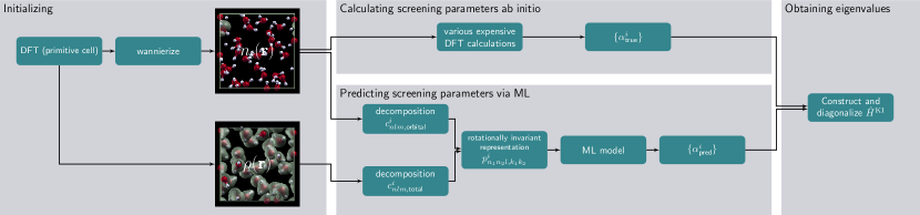
This procedure is visualized in fig. 2.
The third step — that is, calculating the screening parameters — typically dominates the computational cost of the workflow. This is because one has to compute one screening parameter per variational orbital, and for each orbital one must perform a finite difference or DFPT calculation. Of course, if two variational orbitals are symmetrically equivalent, then the same screening parameter can be used for both, and thus for highly symmetric, ordered systems the cost of calculating the screening parameters can be substantially reduced. Nevertheless, for large and/or disordered systems the computation of the screening parameters remains by far the most expensive step of the entire Koopmans workflow.
3 A machine learning model to predict screening parameters
To accelerate Koopmans spectral functional calculations, this work introduces a machine learning (ML) model to predict the screening parameters, thereby avoiding the expensive step of having to calculate them explicitly. Since this ML model only predicts the screening parameters and not the quasi-particle energies directly, the initial DFT and Wannier calculations are still required to define the variational orbitals, as is the final calculation to calculate the quasi-particle energies. This workflow is depicted in fig. 2.
3.1 The descriptors
In order to design a machine learning model, the first thing to do is to define a set of descriptors, for which there are many possible choices. A preliminary study on acenes (presented in Section S1.1 of the Supplementary Information) suggested that there is a strong correlation between the self-Hartree energy of each orbital
| (10) |
and its corresponding screening parameter. This scalar quantity is a measure of how localized an orbital density is, and the fact that the screening parameters were correlated with the self-Hartree energies indicated that it might be possible to predict the screening parameters based on a more complete descriptor of the orbital density.
To convert a real-space orbital density into a compact but information-dense descriptor, we define a local decomposition of the normalized orbital density around the orbital’s center :
| (11) |
where are Gaussian radial basis functions and are real-valued spherical harmonics (following the choice of Ref. 56 and many others). For more details regarding these basis functions, refer to Section S2 of the Supplementary Information.
This choice of basis functions means that the model has four hyperparameters: a maximum order for the radial basis functions , a maximum angular orbital momentum , and two radii and that quantify the radial extent of the Gaussian basis functions. By design, these basis functions will capture orbital densities most accurately in the vicinity of the orbital’s center , and progressively less accurately at larger radii and higher angular momenta. Because the variational orbitals are localized, it is reasonable to assume that most of the relevant information is captured with this local expansion. Choosing these hyperparameters will be influenced by the expected degree of transferability: too large descriptors will lead to more trainable weights and hence usually require more training data. On the other hand, too small descriptors might not capture the information required to accurately predict screening parameters.
In addition to the orbital density , one expects from physical intuition that the screening parameter of orbital , , will also depend on the surrounding electronic density, because these electrons will also contribute to the local electronic screening. For this reason we construct an analogous local descriptor of the total electronic density around the orbital’s center :
| (12) |
Finally, it is important to ensure that the descriptors are invariant with respect to translations and rotations of the entire system, so that the network does not consume training data learning that these operations will not affect the screening parameters. The coefficient vectors defined above are already invariant with respect to translation, but not with respect to rotation. To obtain rotationally invariant input vectors we construct a power spectrum from these coefficient vectors, explicitly coupling coefficients belonging to different shells , as well as coefficients belonging to the total and to the orbital density. The resulting input vector for each orbital is given by the vector containing the coefficients
corresponding to all possible combinations of , , and [57].
3.2 The network
Now that we have defined a descriptor, we must now decide on a machine learning model with which to map the power spectrum of each orbital to its screening parameter. In this work, we use ridge regression [58]. Despite its simplicity, we found that it achieved sufficient accuracy for the case studies with very little training data. By contrast, complex neural networks have more trainable parameters and therefore typically would require more training data. (Of course, this work does not preclude the possibility of employing more sophisticated models in the future.)
4 Results
4.1 The two test systems
This machine learning framework was tested on two systems: liquid water and the halide perovskite \chCsSnI3.
4.1.1 Water
Despite its simple molecular structure, water exhibits very complex behavior. Understanding it better would help us to improve our ability to explain and predict a variety of phenomena in nature and technology and it is therefore an active area of research [22, 59]. For example, accurate values for the ionization potential (IP) and the electron affinity (EA) of water are necessary for a precise description of redox reactions in aqueous systems. These in turn are key to many applications such as (photo-)electrochemical cells [19].
The water system used in this study is a cubic box with a side length of containing 32 water molecules. 20 such snapshots from a molecular dynamics simulation make up the training and test dataset [60]. Each snapshot represents 192 datapoints (i.e. 192 pairs of orbital density descriptors and the corresponding screening parameter calculated ab initio), with the entire dataset corresponding to 3840 datapoints. This test case follows what one could do in order to calculate the spectral properties of water with Koopmans functionals, where one must average across a molecular dynamics trajectory.
4.1.2 \chCsSnI3
Perovskite solar cells are one of the most promising candidates for next-generation solar cells, with reported efficiencies higher than conventional silicon-based solar cells [61]. One of the most prominent perovskite materials for solar cell applications is caesium lead halide (\chCsPbI3) due to its suitable band gap of and its excellent electronic properties. The main drawback of \chCsPbI3 is that lead is toxic, and it is desirable to find more environmentally friendly metals whose substitution does not compromise performance [62]. \chCsSnI3 is one such candidate.
The test system used in this study is a supercell of the 5-atom primitive cell, with length . 20 snapshots of this system with different atomic displacements were generated using the stochastic self-consistent harmonic approximation [44] corresponding to a sampling of the ionic energy surface at . As such, this test case represents how one could calculate the temperature-dependence of the spectral properties of this perovskite, accounting for the anharmonicity of the nuclear motion. Each snapshot represents 200 datapoints, with the entire dataset corresponding to 4000 datapoints.
For more details about these systems and how the snapshots were generated, please refer to Section S3 of the Supplementary Information.
4.2 Computational details
We performed Koopmans calculations on 20 uncorrelated snapshots for each of the two test systems. Screening parameters were computed ab initio for all 20 snapshots; the first 10 snapshots were used when training the models, and the remaining 10 were exclusively reserved for validation. All of the Koopmans functional calculations were performed using Quantum ESPRESSO [63, 64] via the koopmans package. The ridge-regression model was implemented using the scikit-learn library [65]. The descriptor hyperparameters were set to , , , and . An exhaustive grid search over the hyperparameters (with all possible combinations of , , , and ) revealed that for , , and , the mean absolute error in the predicted screening parameters was not very sensitive to the choice of hyperparameters. For the ridge-regression model, the regularization parameter was set to 1 as the result of 10-fold cross-validation, and the input vectors were standardized.
The details of all the calculations are listed in Section S3 of the Supplementary Information, and accompanying data can be found on the Materials Cloud Archive.
4.3 Accuracy
To evaluate the accuracy of a model that predicts screening parameters, we can examine several different metrics. The most obvious quantities to compare are the predicted and the calculated screening parameters. However, these parameters are not physical observables: they are intermediate parameters internal to the Koopmans spectral functional framework. Ultimately, it is much more important that the canonical eigenenergies are accurately predicted. This is because all spectral properties derive from the eigenenergies, and spectral properties are of central interest whenever Koopmans spectral functionals are used.
That said, the eigenenergies are closely related to the screening parameters. As described previously in Section 2, the eigenenergies are the eigenvalues of the matrix , whose elements contain the screening parameters (eq. 9). If all of the orbitals had the same screening parameter then the difference between the Koopmans and DFT eigenvalues would be linear in that screening parameter. For a system with non-uniform screening parameters, the relationship between the eigenvalues and the screening parameters is more complex, with the difference between the Koopmans and DFT eigenvalues becoming a linear mix of the screening parameters of variational orbitals that constitute the canonical orbital in question.
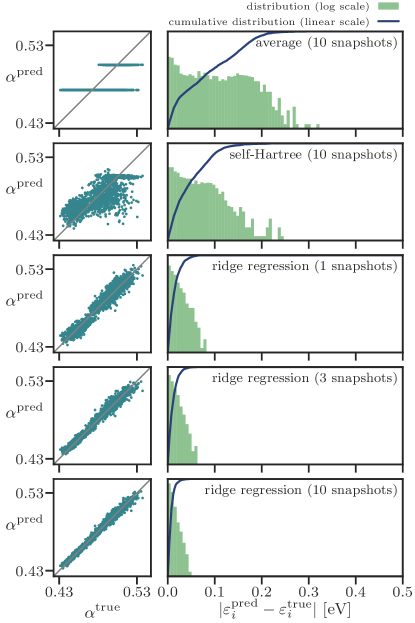
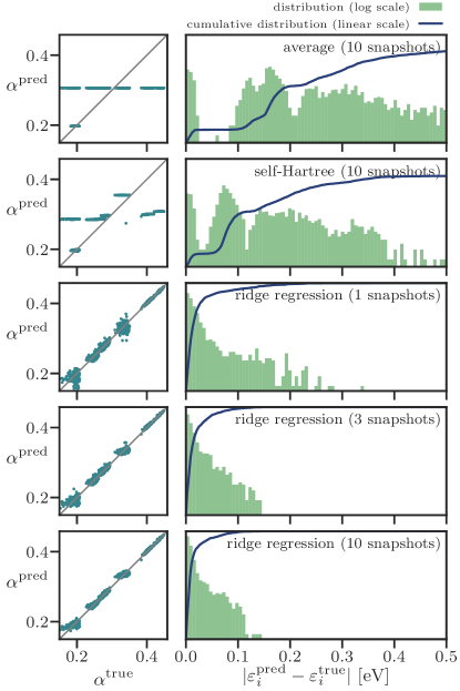
The accuracy of the predicted screening parameters and eigenenergies are shown in fig. 3 for water and in fig. 4 for \chCsSnI3. In these figures, we compare the performance of the ML model against two simplistic benchmark models:
-
•
the average model: here we take the average of the ab initio screening parameters of the training snapshots as the prediction for all screening parameters of the testing snapshots.
-
•
the self-Hartree (sH) model: This is a linear regression model with the self-Hartree energies of each orbital (eq. 10) as input and the screening parameters of each orbital as output (inspired by the preliminary study discussed in Section S1.1 of the Supplementary Information).
We treated occupied and empty states separately in both benchmark models because this gave better results than using one model for the occupied and the empty states together. We note that this treatment of empty states is only possible because the empty states are localized and thus their self-Hartree energies are well-defined. (This was not the case for the preliminary study on acenes presented in the Supplementary Information.)
Given an arbitrary training dataset, the average model is perhaps the simplest possible model for predicting screening parameters. Any successful model must therefore substantially outperform it, and as such it serves as a useful benchmark. figs. 3 and 4 shows the accuracy of the screening parameters and eigenvalues predicted by five different models: the average model (trained on 10 snapshots), the self-Hartree model (trained on 10 snapshots), and the ridge-regression model (trained on 1, 3, and 10 snapshots). The accuracy of all five models was assessed against 10 unseen test snapshots. The errors in the eigenvalues are also tabulated in table 1.
| av. | self-H. | ridge regression | ||||
|---|---|---|---|---|---|---|
| 1 | 3 | 10 | ||||
| water | all | 81.3 | 46.7 | 13.6 | 10.3 | 6.9 |
| VBM | 140.2 | 49.2 | 28.6 | 15.5 | 10.3 | |
| CBM | 8.9 | 9.0 | 5.7 | 3.0 | 2.7 | |
| 133.7 | 45.1 | 30.2 | 16.9 | 10.8 | ||
| CsSnI3 | all | 263.1 | 209.1 | 23.1 | 16.1 | 13.1 |
| VBM | 374.6 | 285.6 | 19.8 | 19.8 | 16.3 | |
| CBM | 7.0 | 6.1 | 17.5 | 9.1 | 7.3 | |
| 372.5 | 284.7 | 30.3 | 25.4 | 19.1 | ||
The ridge-regression model outperformed the average model and the sH model for all systems, both for the screening parameters and the eigenenergies. The mean absolute error of the eigenenergies of the ridge-regression model is below for all test systems already after 1 training snapshot. Meanwhile, the average model and the sH model predict eigenenergies with an average error above for water and even above for \chCsSnI3.
In most applications, one is interested in specific orbital energies and not in quantities averaged over all eigenenergies. Therefore, it is important for the error distribution of the eigenenergies not to have a long tail. In this regard, the ridge-regression model also performs very well. After three training snapshots, ridge regression predicts no single eigenenergy with an error larger than . In comparison, the average model and the sH model predict many eigenenergies with an error larger than ; for \chCsSnI3 many have errors larger than even .
The most important eigenenergies for many applications are the highest occupied molecular orbital (HOMO) and the lowest unoccupied molecular orbital (LUMO) energies, or in bulk systems (such as ) the valence band maximum (VBM) and the conduction band minimum (CBM); in this work, we will treat these terms synonymously. Another important quantity is the band gap (the difference between the VBM and CBM). While the error of the CBM is below the average error in all cases, the error in the VBM is above-average in all cases. This is not a fault of the models but suggests that the screening parameters have a larger influence on the VBM than the CBM. Even still, for most applications the VBM is predicted sufficiently accurately by the ridge regression after 2 or 3 training snapshots. Why the self-Hartree model fails for these two systems after showing promise in the preliminary study of acenes is analysed in Section S1 of the Supplementary Information.
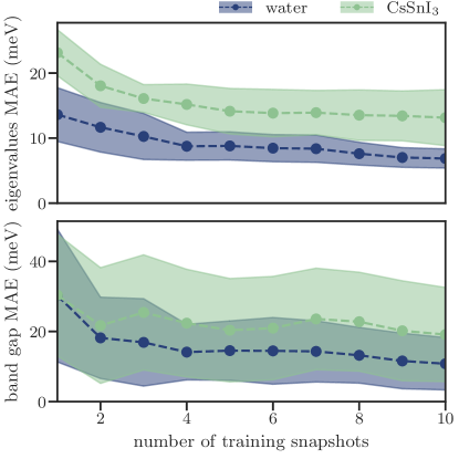
Finally, we examine the convergence of the ridge-regression model with respect to the number of training snapshots in greater detail. Figure 5 shows the convergence of the eigenvalues and the band gap as a function of the number of training snapshots. As we have already seen, the error of the HOMO energy and, correspondingly, the error of the band gap is larger than the mean absolute error. Nevertheless, both quantities become small (i.e. less than 20 meV) already after a few (2 to 4) training snapshots. To put this in perspective, Koopmans functionals typically predict orbital energies and band gaps within of experiment [8, 13] i.e. the error introduced by the ML model is acceptably small, and the accuracy of the predicted band gaps remains state-of-the-art.
4.4 Speed-up
The main goal in developing the ML model is to speed up the calculations with Koopmans spectral functionals while maintaining high accuracy. In the preceding section, we saw that the model achieves a satisfactory level of accuracy after a few training snapshots. In this section, we turn to look at the corresponding speedups.
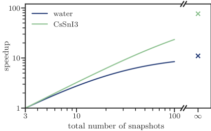
We find that the ratio of the time required for an entire Koopmans calculation when (a) all screening parameters are computed ab initio relative to when (b) all screening parameters are predicted using the ML model is 80 for \chCsSnI3 and 11 for water. However, this does not factor in the cost of training the model in the first place. Figure 6 shows the anticipated speed-ups for performing Koopmans calculations on a given number of snapshots assuming that training requires three snapshots for training (and therefore three snapshots performed ab initio). For performing Koopmans calculations on 20 snapshots one obtains a speedup of roughly 4.4 for the water system and of roughly 6.2 for the \chCsSnI3 system. Because training the model is a one-off cost, for infinitely many configurations we approach the aforementioned 80-fold and 11-fold speedups.
We note that there are scenarios in which the ML model will provide even greater speed-ups than these. For example, the model could be trained on a small supercell and then employed for calculations on larger supercells. Because the cost of DFT calculations scales cubically with system size (cf. linearly with the number of snapshots), machine-learning promises even greater speed-ups for such schemes. We note that this approach is only possible because the descriptors are spatially localized and therefore invariant with respect to the system size.
5 Conclusions
This work presented a machine learning framework to predict electronic screening parameters via ridge regression performed on translationally- and rotationally-invariant power spectrum descriptors of orbital densities. This framework is able to predict the screening parameters for Koopmans spectral functionals with sufficient accuracy and with sufficiently little training data so as to dramatically decrease the computational cost of these calculations while maintaining their state-of-the-art accuracy, as demonstrated on the test cases of liquid water and the halide perovskite \chCsSnI3.
It is somewhat surprising that it is possible to accurately predict screening parameters directly from orbital densities, because the screening parameters are not explicitly determined by orbital densities themselves but instead are related to the response of these densities (refer back to eq. 8). Nevertheless, for the systems studied in this work the relationship between the orbital’s density (plus the surrounding electron density) and its screening parameter learned by a ridge-regression model gives very accurate predictions of the screening parameters for orbitals it has never seen before — albeit for the same system; we do not expect the model to be transferable across different systems.
Work is already ongoing to use this machine-learning framework to predict the temperature-dependent spectral properties of materials of scientific interest.
Supplementary information
The Supplementary information contains results that explore the correlation between the screening parameters and self-Hartree energies, further details on the basis functions behind the descriptors, detailed descriptions of the two test systems, and the computational setup used to model each.
Acknowledgements The authors thank Nicola Colonna, Lorenzo Monacelli, and Martin Uhrin for helpful discussions. EL gratefully acknowledges financial support from the Swiss National Science Foundation (grant numbers 179138 and 213082). This research was also supported by the NCCR MARVEL, a National Centre of Competence in Research, funded by the Swiss National Science Foundation (grant number 205602).
Author contributions YS: Methodology, Software, Validation, Investigation, Writing – Original Draft. SL: Supervision, Writing – Review & Editing. NM: Conceptualization, Supervision, Writing – Review & Editing. EL: Conceptualization, Methodology, Software, Supervision, Writing – Review & Editing
Competing interests The authors declare no competing interests.
Data availability The data underpinning this work can be downloaded from to the Materials Cloud Archive.
Code availability The code used to generate the results of this paper is open-source and is available at github.com/epfl-theos/koopmans. Version 1.0.0 of the code was used.
References
- \bibcommenthead
- [1] Marzari, N., Ferretti, A. & Wolverton, C. Electronic-structure methods for materials design. Nat. Mater. 20, 736–749 (2021).
- [2] Dabo, I., Cococcioni, M. & Marzari, N. Non-Koopmans Corrections in Density-functional Theory: Self-interaction Revisited (2009).
- [3] Dabo, I. et al. Koopmans’ condition for density-functional theory. Phys. Rev. B 82, 115121 (2010).
- [4] Dabo, I., Ferretti, A. & Marzari, N. in Piecewise Linearity and Spectroscopic Properties from Koopmans-Compliant Functionals (eds Di Valentin, C., Botti, S. & Cococcioni, M.) First Principles Approaches to Spectroscopic Properties of Complex Materials 193–233 (Springer, Berlin, Heidelberg, 2014).
- [5] Borghi, G., Ferretti, A., Nguyen, N. L., Dabo, I. & Marzari, N. Koopmans-compliant functionals and their performance against reference molecular data. Phys. Rev. B 90, 075135 (2014).
- [6] Ferretti, A., Dabo, I., Cococcioni, M. & Marzari, N. Bridging density-functional and many-body perturbation theory: Orbital-density dependence in electronic-structure functionals. Phys. Rev. B 89, 195134 (2014).
- [7] Borghi, G., Park, C. H., Nguyen, N. L., Ferretti, A. & Marzari, N. Variational minimization of orbital-density-dependent functionals. Phys. Rev. B - Condens. Matter Mater. Phys. 91, 155112 (2015).
- [8] Nguyen, N. L., Colonna, N., Ferretti, A. & Marzari, N. Koopmans-compliant spectral functionals for extended systems. Phys. Rev. X 8, 021051 (2018).
- [9] Colonna, N., Nguyen, N. L., Ferretti, A. & Marzari, N. Screening in orbital-density-dependent functionals. J. Chem. Theory Comput. 14, 2549–2557 (2018).
- [10] De Gennaro, R., Colonna, N., Linscott, E. & Marzari, N. Bloch’s theorem in orbital-density-dependent functionals: Band structures from Koopmans spectral functionals. Phys. Rev. B 106, 035106 (2022).
- [11] Colonna, N., De Gennaro, R., Linscott, E. & Marzari, N. Koopmans spectral functionals in periodic boundary conditions. J. Chem. Theory Comput. (2022).
- [12] Linscott, E. B. et al. Koopmans: An Open-Source Package for Accurately and Efficiently Predicting Spectral Properties with Koopmans Functionals. J. Chem. Theory Comput. 19, 7097–7111 (2023).
- [13] Colonna, N., Nguyen, N. L., Ferretti, A. & Marzari, N. Koopmans-compliant functionals and potentials and their application to the GW100 test set. J. Chem. Theory Comput. 15, 1905–1914 (2019).
- [14] Dabo, I. et al. Donor and acceptor levels of organic photovoltaic compounds from first principles. Phys. Chem. Chem. Phys. 15, 685–695 (2013).
- [15] Nguyen, N. L., Borghi, G., Ferretti, A., Dabo, I. & Marzari, N. First-principles photoemission spectroscopy and orbital tomography in molecules from koopmans-compliant functionals. Phys. Rev. Lett. 114, 166405 (2015).
- [16] Nguyen, N. L., Borghi, G., Ferretti, A. & Marzari, N. First-principles photoemission spectroscopy of DNA and RNA nucleobases from koopmans-compliant functionals. J. Chem. Theory Comput. 12, 3948–3958 (2016).
- [17] Schubert, Y., Marzari, N. & Linscott, E. Testing Koopmans spectral functionals on the analytically solvable Hooke’s atom. J. Chem. Phys. 158, 144113 (2023).
- [18] Elliott, J. D., Colonna, N., Marsili, M., Marzari, N. & Umari, P. Koopmans Meets Bethe–Salpeter: Excitonic Optical Spectra without GW. J. Chem. Theory Comput. 15, 3710–3720 (2019).
- [19] Stojkovic, M., Marzari, N. & Linscott, E. Predicting the suitability of photocatalysts for water splitting using Koopmans spectral functionals: The case of TiO2 polymorphs (2024).
- [20] Marrazzo, A. & Colonna, N. Spin-dependent interactions in orbital-density-dependent functionals: Non-collinear Koopmans spectral functionals (2024).
- [21] Ingall, J. E., Linscott, E., Colonna, N., Page, A. J. & Keast, V. J. Accurate and Efficient Computation of the Fundamental Bandgap of the Vacancy-Ordered Double Perovskite Cs2TiBr6. J. Phys. Chem. C (2024).
- [22] de Almeida, J. M. et al. Electronic structure of water from koopmans-compliant functionals. J. Chem. Theory Comput. 17, 3923–3930 (2021).
- [23] Carleo, G. et al. Machine learning and the physical sciences. Rev. Mod. Phys. 91, 045002 (2019).
- [24] Ceriotti, M., Clementi, C. & Anatole von Lilienfeld, O. Introduction: Machine Learning at the Atomic Scale. Chem. Rev. 121, 9719–9721 (2021).
- [25] Dral, P. O. & Barbatti, M. Molecular excited states through a machine learning lens. Nat Rev Chem 5, 388–405 (2021).
- [26] Westermayr, J. & Marquetand, P. Machine learning for electronically excited states of molecules. Chem. Rev. 121, 9873–9926 (2021).
- [27] Cignoni, E. et al. Electronic Excited States from Physically Constrained Machine Learning. ACS Cent. Sci. 10, 637–648 (2024).
- [28] Yu, M., Yang, S., Wu, C. & Marom, N. Machine learning the Hubbard U parameter in DFT+U using Bayesian optimization. npj Comput Mater 6, 1–6 (2020).
- [29] Yu, W. et al. Active Learning the High-Dimensional Transferable Hubbard U and V Parameters in the DFT + U + V Scheme. J. Chem. Theory Comput. 19, 6425–6433 (2023).
- [30] Cai, G. et al. Predicting structure-dependent Hubbard U parameters via machine learning. Mater. Futures 3, 025601 (2024).
- [31] Uhrin, M., Zadoks, A., Binci, L., Marzari, N. & Timrov, I. Machine learning Hubbard parameters with equivariant neural networks (2024).
- [32] Dong, S. S., Govoni, M. & Galli, G. Machine learning dielectric screening for the simulation of excited state properties of molecules and materials. Chem. Sci. 12, 4970–4980 (2021).
- [33] Montavon, G. et al. Machine learning of molecular electronic properties in chemical compound space. New J. Phys. 15, 095003 (2013).
- [34] Brockherde, F. et al. Bypassing the Kohn-Sham equations with machine learning. Nat Commun 8, 872 (2017).
- [35] Welborn, M., Cheng, L. & Miller, T. F. I. Transferability in machine learning for electronic structure via the molecular orbital basis. J. Chem. Theory Comput. 14, 4772–4779 (2018).
- [36] Schleder, G. R., Padilha, A. C. M., Acosta, C. M., Costa, M. & Fazzio, A. From DFT to machine learning: Recent approaches to materials science–a review. J. Phys. Mater. 2, 032001 (2019).
- [37] Ryczko, K., Strubbe, D. A. & Tamblyn, I. Deep learning and density-functional theory. Phys. Rev. A 100, 022512 (2019).
- [38] Noé, F., Tkatchenko, A., Müller, K.-R. & Clementi, C. Machine learning for molecular simulation. Annu. Rev. Phys. Chem. 71, 361–390 (2020).
- [39] Häse, F., Roch, L. M., Friederich, P. & Aspuru-Guzik, A. Designing and understanding light-harvesting devices with machine learning. Nat Commun 11, 4587 (2020).
- [40] Sutton, C. et al. Identifying domains of applicability of machine learning models for materials science. Nat Commun 11, 4428 (2020).
- [41] Bogojeski, M., Vogt-Maranto, L., Tuckerman, M. E., Müller, K.-R. & Burke, K. Quantum chemical accuracy from density functional approximations via machine learning. Nat Commun 11, 5223 (2020).
- [42] Ghosh, K. et al. Deep Learning Spectroscopy: Neural Networks for Molecular Excitation Spectra. Adv. Sci. 6, 1801367 (2019).
- [43] Zacharias, M. & Giustino, F. Theory of the special displacement method for electronic structure calculations at finite temperature. Phys. Rev. Research 2, 013357 (2020).
- [44] Monacelli, L. & Mauri, F. Time-dependent self-consistent harmonic approximation: Anharmonic nuclear quantum dynamics and time correlation functions. Phys. Rev. B 103, 104305 (2021).
- [45] Janak, J. F. Proof that E/ni = in density-functional theory. Phys. Rev. B 18, 7165–7168 (1978).
- [46] Cohen, A. J., Mori-Sánchez, P. & Yang, W. Challenges for density functional theory. Chem. Rev. 112, 289–320 (2012).
- [47] Pederson, M. R., Heaton, R. A. & Lin, C. C. Local-density Hartree–Fock theory of electronic states of molecules with self-interaction correction. J. Chem. Phys. 80, 1972–1975 (1984).
- [48] Pederson, M. R., Heaton, R. A. & Lin, C. C. Density-functional theory with self-interaction correction: Application to the lithium moleculea). J. Chem. Phys. 82, 2688–2699 (1985).
- [49] Pederson, M. R. & Lin, C. C. Localized and canonical atomic orbitals in self-interaction corrected local density functional approximation. J. Chem. Phys. 88, 1807–1817 (1988).
- [50] Heaton, R. A., Harrison, J. G. & Lin, C. C. Self-interaction correction for density-functional theory of electronic energy bands of solids. Phys. Rev. B 28, 5992–6007 (1983).
- [51] Marzari, N., Mostofi, A. A., Yates, J. R., Souza, I. & Vanderbilt, D. Maximally localized Wannier functions: Theory and applications. Rev. Mod. Phys. 84, 1419–1475 (2012).
- [52] Stengel, M. & Spaldin, N. A. Self-interaction correction with Wannier functions. Phys. Rev. B 77, 155106 (2008).
- [53] Goedecker, S. & Umrigar, C. J. Critical assessment of the self-interaction-corrected–local-density-functional method and its algorithmic implementation. Phys. Rev. A 55, 1765–1771 (1997).
- [54] Körzdörfer, T., Kümmel, S. & Mundt, M. Self-interaction correction and the optimized effective potential. J Chem Phys 129, 014110 (2008).
- [55] Vydrov, O. A. & Scuseria, G. E. Ionization potentials and electron affinities in the Perdew-Zunger self-interaction corrected density-functional theory. J Chem Phys 122, 184107 (2005).
- [56] Himanen, L. et al. DScribe: Library of descriptors for machine learning in materials science. Comput. Phys. Commun. 247, 106949 (2020).
- [57] Bartók, A. P., Kondor, R. & Csányi, G. On representing chemical environments. Phys. Rev. B 87, 184115 (2013).
- [58] Hoerl, A. E. & Kennard, R. W. Ridge regression: Biased estimation for nonorthogonal problems. Technometrics 12, 55–67 (1970).
- [59] Gaiduk, A. P., Pham, T. A., Govoni, M., Paesani, F. & Galli, G. Electron affinity of liquid water. Nat Commun 9, 247 (2018).
- [60] Chen, W., Ambrosio, F., Miceli, G. & Pasquarello, A. Ab initio electronic structure of liquid water. Phys. Rev. Lett. 117, 186401 (2016).
- [61] Min, H. et al. Perovskite solar cells with atomically coherent interlayers on SnO2 electrodes. Nature 598, 444–450 (2021).
- [62] Li, Z., Zhou, F., Wang, Q., Ding, L. & Jin, Z. Approaches for thermodynamically stabilized CsPbI3 solar cells. Nano Energy 71, 104634 (2020).
- [63] Giannozzi, P. et al. QUANTUM ESPRESSO: A modular and open-source software project for quantum simulations of materials. J. Phys. Condens. Matter 21, 395502 (2009).
- [64] Giannozzi, P. et al. Advanced capabilities for materials modelling with Quantum ESPRESSO. J. Phys. Condens. Matter 29, 465901 (2017).
- [65] Pedregosa, F. et al. Scikit-learn: Machine Learning in Python. J. Mach. Learn. Res. 12, 2825–2830 (2011).