A Law Limit Theorem for a sequence of random variables

Abstract.

An application of Levy’s continuity theorem and Hankel transform allow us to establish a law limit theorem for the sequence $V_{n}=f(U)\sin(nU)$, where $U$ is uniformly distributed in $(0,1)$ and $f$ a given function. Further, we investigate the inverse problem by specifying a limit distribution and look for the suitable function $f$ ensuring the convergence in law to the specified distribution. Our work recovers and extends existing similar works, in particular we make it possible to sample from known laws including Gaussian and Cauchy distributions.

1. Introduction and preliminaries

Studying the asymptotic behavior of sequences of random variables has always been crucial and a fundamental tool for theoretical research and practical applications in fields such as probability, statistics, finance and engineering to mention few. See [12, 14, 8, 3] for more details. In these areas, the Law of Large Numbers and the Central Limit Theorems play crucial role. In recent years, due to the huge development in communication and information fields, there is a growing need for simulations using specific distributions in a wide range of disciplines. See [9, 4, 19, 20, 15, 11] and the references therein. This paper aims to follow in this direction and explore a law limit theorem for a specific sequence of random variables given by (2.2). This exploration uses two key tools, namely Levy’s continuity theorem together with Hankel transform and yields two main results. The first main result gives sufficient conditions on the parameter function $f$ under which the convergence in law of $V_{n}[f]$ holds. (See Theorem 2.2). The second main result investigates the inverse problem. More precisely, starting from a suitable given density, we give sufficient conditions allowing us to construct a function $f$ such that the sequence $V_{n}[f]$ given by (2.2) converges in law to our specified limiting distribution (See Theorem 2.5).

We point out here that a version of Theorem 2.2 has been established in [2] in the particular case $f(u)=\sqrt{-2\ln(u)}$ which led to the normal distribution using direct calculations. Our work recover their result by exploring a general framework and giving the convergence problem a wide perspective. Indeed, by investigating this general problem, the direct and inverse one, we can obtain a convergence in law to a wide class of districbutions including the Cauchy distribution as shown in this paper.

The remaining of this section serves to introduce some notations and definitions needed for the sequel. Section 2 sets our main results, namely Theorem 2.1, Theorem 2.2 and Theorem 2.5. In Section 3 we apply our results by giving some examples to illustrate the practical aspect of our work. Finally, in Section 4, we summarize our findings and suggest some directions for future work.

Throughout this paper, $\mathbb{N}=\left\{0,1,2,\dots\right\}$ , $\mathbb{Z}=\left\{\dots,-2,-1,0,1,2,\dots\right\}$ and $\mathbb{R}^{d}$ is equipped with its standard scalar product and Euclidean norm, denoted in the sequel respectively by $\left\langle,\right\rangle$ and $\left\|{\ }\right\|$.

The sets $L^{1}(\mathbb{R}^{d})$ and $L^{1}_{loc}((a,b))$, $(a,b)\subset\mathbb{R}$, keep their standard meaning in this paper with respect to Lebesgue measure.

For $\psi:\mathbb{R}^{d}\to\mathbb{C}$, with $\psi\in L^{1}(\mathbb{R}^{d})$, $d\geq 1$, its Fourier transform is given by

$$\mathcal{F}_{d}(\psi)(y)=\frac{1}{(2\pi)^{d/2}}\int_{\mathbb{R}^{d}}\psi(x)e^{-i\left\langle x,y\right\rangle}dx.$$

Following [18], Bessel function of the first kind and order $n\in\mathbb{Z}$, denoted hereafter by $J_{n}$ is given by its integral expression

$$J_{n}(x)={\frac{1}{2\pi}}\int_{-\pi}^{\pi}e^{i(x\sin(u)-nu)}\,du,\quad x\in\mathbb{R}.$$ (1.1)

See [1, 22] for details on Bessel functions.

In particular, we see from (1.1) that for all $n\in\mathbb{Z}$, $J_{n}$ is bounded in $\mathbb{R}$ and

$$J_{-n}(x)=(-1)^{n}J_{n}(x),\quad\forall x\in\mathbb{R},$$ (1.2)

and that the function $J_{0}$, which plays an important role in this paper, is even. Morover, for all $n\in\mathbb{N}$, $J_{n}$ admits the series expansion

$$J_{n}(x)=\sum_{k=0}^{\infty}\frac{(-1)^{k}}{k!(k+n)!}\left({\frac{x}{2}}\right)^{2k+n},\quad x\in\mathbb{R}.$$ (1.3)

According to Watson [22, Page 24] we have

$$\left|{J_{n}(x)}\right|\leq\frac{\left|{x}\right|^{n}}{2^{n}\Gamma(n+1/2)\Gamma(1/2)}$$ (1.4)

for all $x\in\mathbb{R}$ and $n\in\mathbb{N}$.

The Hankel transform of order 0 of a function $f:(0,+\infty)\to\mathbb{R}$ is given by:

$$\mathcal{H}_{0}(f)(t)=\int_{0}^{\infty}f(r)J_{0}(rt)\,r\operatorname{d}\!r,\quad t\in\mathbb{R}$$ (1.5)

provided that $x\mapsto xf(x)\in L^{1}((0,+\infty))$. Following [22, Page 456] ( See also [16, Theorem 19]), if $f$ is further of bounded variation in each bounded sub-interval of $(0,+\infty)$ and $x\mapsto\sqrt{x}f(x)\in L^{1}((0,+\infty))$, then $f=\mathcal{H}_{0}(\mathcal{H}_{0}(f))$. That is

$$f(r)=\int_{0}^{\infty}\mathcal{H}_{0}(f)(t)J_{0}(rt)\,t\operatorname{d}\!t,\quad r\geq 0.$$ (1.6)

In [13], a relationship between the Fourier transform of radial functions in $\mathbb{R}^{2}$ and their Hankel transform is given.

Theorem 1.1.

[13]. Let $w\in L^{1}(\mathbb{R}^{2})$ be radial with $w(x)=G(\left\|{x}\right\|)$. Then for all $y\in\mathbb{R}^{2}$ we have

$$\mathcal{F}_{2}(w)(y)=\mathcal{H}_{0}(G)(\left\|{y}\right\|).$$

One precious tool in this paper is Levy continuity’s theorem (see [7]), which turns to be the corner stone in the proof of Theorem 2.2.

Theorem 1.2 (Lévy’s continuity Theorem).

Consider a sequence of random variables $X_{n}$, $n\geq 1$, and define the sequence of corresponding characteristic functions

$$\varphi_{n}(t):=\mathbb{E}\left(e^{itX_{n}}\right),\quad(t\in\mathbb{R}),$$

where $\mathbb{E}$ is the expected value operator. If the sequence $\varphi_{n}$ converges point wise to some function $\varphi$ which is continuous at $t=0$, then the sequence $X_{n}$ converges in distribution to some random variable $X$ and $\varphi$ is the characteristic function of the random variable $X$.

The next result, useful for its own, turns out to be crucial for our developments. Up to our knowledge the formula (1.8) exists nowhere.

Proposition 1.3.

Let $w\in\mathbb{R}$. Then we have

$$e^{iw\sin(x)}=\sum_{k=-\infty}^{\infty}J_{k}(w)e^{ikx}$$ (1.7)

for all $x\in\mathbb{R}$. Moreover,

$$\frac{w^{2}}{2}=\sum_{k=-\infty}^{\infty}k^{2}(J_{k}(w))^{2}$$ (1.8)

Proof.

For $w\in\mathbb{R}$ fixed, define the function

$$h(x):=e^{iw\sin(x)},\quad x\in\mathbb{R}.$$

Keeping the formula (1.1) in mind, the Fourier series expansion of $h$ gives us

$$h(x)=\sum_{k=-\infty}^{\infty}J_{k}(w)e^{ikx}$$

for all $x\in\mathbb{R}$ and this proves our first claim.

In other hand, from (1.2) and (1.4) we have $\sum_{k=-\infty}^{\infty}\left|{kJ_{k}(w)}\right|<+\infty$, which allows us to derive with respect to $x$ in (1.7) and get

$$w\cos(x)e^{iw\sin(x)}=\sum_{k=-\infty}^{\infty}kJ_{k}(w)e^{ikx}$$

for all $x\in\mathbb{R}$. Using Parseval identity, we deduce that

$$\frac{w^{2}}{2\pi}\int_{-\pi}^{\pi}\left|{\cos(x)}\right|^{2}dx=\sum_{k=-\infty}^{\infty}k^{2}(J_{k}(w))^{2}$$

which is the second desired result.

∎

Before leaving this section we establish a well known simple lemma needed for the sequel.

Lemma 1.4.

Fix $a>0$ and set

$$\theta_{a}(t)=\frac{1}{t^{2}+a^{2}},\quad t\in\mathbb{R}.$$

Then we have $\mathcal{F}_{1}(\theta_{a})(t)=\frac{\sqrt{\pi}}{a\sqrt{2}}e^{-a\left|{t}\right|}$ for all $t\in\mathbb{R}$.

Proof.

Noting that

$$\mathcal{F}_{1}(e^{-a\left|{u}\right|})(t)=a\sqrt{\frac{2}{\pi}}\theta_{a}(t)$$

the result follows using the inverse Fourier transform. ∎

Now we have all needed ingredients for our developments.

2. Main Results

We begin our developments by the first main result in this paper. It is the corner stone on which all the other results are constructed.

Theorem 2.1.

Consider $f:(a,b)\subset\mathbb{R}\to\mathbb{R}$, with $f\in L^{1}((a,b))$. Then we have

$$\lim_{n\to\infty}\int_{a}^{b}e^{if(u)\sin(nu)}du=\int_{a}^{b}J_{0}(f(u))du.$$

Further, if $a,b\in\mathbb{R}$ then the result holds with $f\in L^{1}_{loc}(a,b)$ only.

Proof.

Let $u\in(a,b)$. Taking $w=f(u)$ in Proposition 1.3 and letting $x=nu$ in (1.7) we get

$$e^{if(u)\sin(nu)}=\sum_{k=-\infty}^{\infty}J_{k}(f(u))e^{iknu}.$$

Whence,

$$\int_{a}^{b}e^{if(u)\sin(nu)}du-\int_{a}^{b}J_{0}(f(u))du=\int_{a}^{b}\left(\sum_{{}^{k=-\infty}_{k\neq 0}}^{\infty}J_{k}(f(u))e^{iknu}\right)du$$

We assume first here that $f\in L^{1}((a,b))$. Using Cauchy-Schwartz inequality together with (1.8), yields

$$\int_{a}^{b}\sum_{{}^{k=-\infty}_{k\neq 0}}^{\infty}\left|{J_{k}(f(u))}\right|du\leq C_{1}\int_{a}^{b}\left(\sum_{{}^{k=-\infty}_{k\neq 0}}^{\infty}(kJ_{k}(f(u)))^{2}\right)^{1/2}\leq C_{2}\int_{a}^{b}\left|{f(u)}\right|du$$ (2.1)

where $C_{1}=\left(2\sum_{k=1}^{\infty}\frac{1}{k^{2}}\right)^{1/2}$ and $C_{2}=\frac{C_{1}}{\sqrt{2}}$.

Taking $f\in L^{1}((a,b))$ into account allows us to write

$$\int_{a}^{b}e^{if(u)\sin(nu)}du-\int_{a}^{b}J_{0}(f(u))du=\sum_{{}^{k=-\infty}_{k\neq 0}}^{\infty}\int_{a}^{b}J_{k}(f(u))e^{iknu}du.$$

Finally, by Riemann-Lebesgue lemma together with (2.1), we get that

$$\lim_{n\to\infty}\int_{a}^{b}e^{if(u)\sin(nu)}du=\int_{a}^{b}J_{0}(f(u))du.$$

Assume now that $a,b\in\mathbb{R}$ and $f\in L^{1}_{loc}(a,b)$. Fix $\epsilon>0$ and choose $\alpha,\beta$ such that

$$\left|{a-\alpha}\right|<\epsilon\quad\text{and}\quad\left|{b-\beta}\right|<\epsilon.$$

Then for all $n\in\mathbb{N}$ we have

$$\left|{\int_{a}^{b}e^{if(u)\sin(nu)}du-\int_{a}^{b}J_{0}(f(u))du}\right|\leq\left|{\int_{\alpha}^{\beta}e^{if(u)\sin(nu)}du-\int_{\alpha}^{\beta}J_{0}(f(u))du}\right|+4\epsilon.$$

Our result follows now using the previous case and the proof is complete. ∎

In the sequel, $U$ denotes a random variable uniformly distributed in the interval $[0,1]$. For $f:(0,1)\to\mathbb{R}$ define the random variable $V_{n}[f]$ given by

$$V_{n}=V_{n}[f]:=f(U)\sin(nU),\quad n=0,1,2,\dots$$ (2.2)

An application of Theorem 2.1 and Levy’s theorem 1.2 all together lead to our second main result.

Theorem 2.2.

Assume that the function $f$ in (2.2) satisfies $f\in L^{1}_{loc}(0,1)$.

Then the sequence of random variables $V_{n}[f]$ defined by (2.2) converges in law to a random variable $V$ such that

$$\mathbb{E}(e^{itV})=\int_{0}^{1}J_{0}(tf(u))du,\quad\forall t\in\mathbb{R}.$$

Proof.

Since $f\in L^{1}_{loc}((0,1))$ then by application of Theorem 2.1 we get

$$\lim_{n\to\infty}\mathbb{E}(e^{itf(U)\sin(nU)})=\lim_{n\to\infty}\int_{0}^{1}e^{itf(u)\sin(nu)}du=\int_{0}^{1}J_{0}(tf(u))du$$

for all $t\in\mathbb{R}$. The function $\varphi$ defined

$$\varphi(t):=\int_{0}^{1}J_{0}(tf(u))du,\quad t\in\mathbb{R}$$ (2.3)

is continuous, by consequence appealing to Levy Theorem 1.2 there exists a random variable $V$ such that $V_{n}[f]$ converges in law to $V$ and

$$\mathbb{E}(e^{itV})=\int_{0}^{1}J_{0}(tf(u))du,\quad t\in\mathbb{R},$$

and the proof is complete. ∎

The next result gives sufficient conditions on the function $f$ so that the random variable $V$ in Theorem 2.2 admits a probability density function.

Corollary 2.3.

We reuse the notations of Theorem 2.2 and assume that $f$ is a strictly monotone bijection of class $C^{1}$ from $(0,1)$ into some $(a,b)\subset(0,+\infty)$ such that $f\in L^{1}_{loc}(0,1)$. Let

$$h(u):=\epsilon_{f}\chi_{(a,b)}(u)\frac{(f^{-1})^{\prime}(u)}{u},\quad u\in(0,+\infty)$$

with $\chi_{(a,b)}$ being the characteristic function of the set $(a,b)$, and $\epsilon_{f}=1$ if $f$ is increasing and $\epsilon_{f}=-1$ if $f$ is decreasing.

Assume that the map $v:=\mathcal{H}_{0}(h)$ satisfies $v\in L^{1}(\mathbb{R})$. Then the sequence of random variables $V_{n}[f]$ defined by (2.2) converges in law to a random variable $V$ having $\frac{1}{\sqrt{2\pi}}\mathcal{F}_{1}(v)$ as a probability density function.

Proof.

From Theorem 2.2 we have

$$\mathbb{E}(e^{itV})=\epsilon_{f}\int_{a}^{b}J_{0}(tu)(f^{-1})^{\prime}(u)du=\int_{0}^{\infty}J_{0}(tu)h(u)udu=v(t)$$

for all $t\in\mathbb{R}$. By hypothesis $v\in L^{1}(\mathbb{R})$, thus the probability density function of $V$ is $\frac{1}{\sqrt{2\pi}}\mathcal{F}_{1}(v)$ and this ends the proof. ∎

Remark 2.4.

Keeping Corollary 2.3 notations in mind, it is worth noting that if we assume $h(\left\|{\cdot}\right\|)\in L^{1}(\mathbb{R}^{2})$, then by Theorem 1.1 we get $v(t)=\mathcal{F}_{2}(h(\left\|{\cdot}\right\|))(\left|{t}\right|e_{1})$ for all $t\in\mathbb{R}$ where $e_{1}=(1,0)$.

Now we come to our third main result in this paper which we will refer to by the inverse problem. Our objective here is to give sufficient conditions so that the inverse problem admits a solution. More precisely, given a suitable map $\psi\in L^{1}(\mathbb{R})$, we give sufficient conditions ensuring that there exists a function $f$ such that the sequence $V_{n}[f]$ given by (2.2) converges in law to a random variable $V$ having $\frac{1}{\sqrt{2\pi}}\mathcal{F}_{1}(\psi)$ as probability density function. Solving this problem is particularly useful when one wants to sample some data from a given none standard distribution. See Section 3 for a an example of the Cauchy distribution using this inverse problem.

Before stating our result, it is worth noting that following Theorem 2.2, there are some conditions that have to be fulfilled by the function $\psi$. This leads us to investigate our inverse problem within the class of functions $\psi:\mathbb{R}\to\mathbb{R}$ satisfying the following, not restrictive, properties denoted hereafter by ($\mathcal{L}$).

$$\left\{\begin{array}[]{ll}1.&\psi\in C^{1}(\mathbb{R}),\\[3.0pt] 2.&\psi,\sqrt{t}\psi(t)\text{ and }t\psi(t)\text{ are in }L^{1}((0,\infty)),\\[3.0pt] 3.&\psi\text{ even, non negative with }\psi(0)=1.\end{array}\right. \mathcal{L}$$ ()

For a function $\psi$ satisfying ($\mathcal{L}$) we set

$$k_{\psi}(t):=1-\int_{0}^{t}u\mathcal{H}_{0}(\psi)(u)du,\quad t\geq 0.$$ (2.4)

Appealing to ($\mathcal{L}$) and (1.6) we see that $k_{\psi}$ is a decreasing bijection from $(0,+\infty)$ into $(0,1)$. Moreover, we have the following:

Theorem 2.5.

Let $\psi$ be a function satisfying ($\mathcal{L}$) such that $(k_{\psi})^{-1}\in L^{1}_{loc}(0,1)$. Then the sequence of random variables $V_{n}[(k_{\psi})^{-1}]$ given by (2.2) converges in law to a random variable $V$ having $\frac{1}{\sqrt{2\pi}}\mathcal{F}_{1}(\psi)$ as probability density function.

Proof.

Define the sequence of random variables $V_{n}[f]$ as in (2.2) with $f(t)=(k_{\psi})^{-1}(t)$, $t\in(0,1)$. From 2.2, we get that the sequence $V_{n}[f]$ converges in law to a random variable $V$ with

$$\mathbb{E}(e^{itV})=-\int_{0}^{\infty}J_{0}(tu)(f^{-1})^{\prime}(u)du=-\int_{0}^{\infty}J_{0}(tu)k_{\psi}^{\prime}(u)du,$$

for all $t\in\mathbb{R}$. Using the expression (2.4) leads to

$$\mathbb{E}(e^{itV})=\mathcal{H}_{0}(\mathcal{H}_{0}(\psi))(t),$$

for all $t\in\mathbb{R}$. Since $\psi$ satisfies ($\mathcal{L}$) the Hankel transform inversion formula (1.6) gives us

$$\mathcal{H}_{0}(\mathcal{H}{{}_{0}(\psi)})(t)=\psi(t),\quad\forall t\geq 0.$$

Taking into account that $\psi$ is even, the latter equality holds for all $t\in\mathbb{R}$, that is

$$\mathbb{E}(e^{itV})=\psi(t),\quad\forall t\in\mathbb{R}.$$

Thus $\frac{1}{\sqrt{2\pi}}\mathcal{F}_{1}(\psi)$ is the probability density function for $V$ and the proof is complete. ∎

3. Applications

This section is devoted to some applications using the results and notations of Section 2. Namely, we will use two kind of applications. The first one, which we will call “Direct problem”, consists of starting from a given function $f$ and use the results of Theorem 2.2 or Corollary 2.3. The second application, which we will call “Inverse problem”, will starts from a given map $\psi$ and use the results of Theorem 2.5 to construct the function $f$ in (2.2).

Example 3.1.

In this example we use the notations and results of Corollary 2.3 and consider $f$ given by

$$f(x)=\sqrt{-2\ln(x)},\quad x\in(0,1).$$

We see that $f\in L^{1}((0,1))$, and is a decreasing bijection of class $C^{1}$ from $(0,1)$ to $(0,+\infty)$. Moreover, by setting

$$h(u):=-\frac{(f^{-1})^{\prime}(u)}{u}=e^{-u^{2}/2},\quad u>0$$

direct application of Corollary 2.3 leads to

$$\psi(t)=e^{-t^{2}/2},\quad t\in\mathbb{R}$$

and t that the sequence $V_{n}[f]$ defined by

$$V_{n}=\sqrt{-2\ln(U)}\sin(nU),\quad n\in\mathbb{N}$$

converges in law to the normal Gaussian. Thus, we recover the result in [2].

Example 3.2.

In this example we illustrate the technique of inverse problem mentioned above for two given distributions.

1. We consider the Gaussian distribution density $\psi(t)=e^{-t^{2}/2}$, $t\in\mathbb{R}$. Following Theorem 2.5, the candidate function $f:=(k_{\psi})^{-1}$ is solution of

   $$k_{\psi}^{\prime}(t)=-t\mathcal{H}_{0}(\psi)(t),\quad t>0.$$

   According to [13, Table 9.1] we have

   $$k_{\psi}^{\prime}(t)=-te^{-t^{2}/2},\quad t>0$$

   from which it follows that

   $$f(u)=(k_{\psi})^{-1}(u)=\sqrt{-2\ln(u)},\quad u\in(0,1).$$

   Thus, we recover again the result in [2] using the inverse problem.

2. Here the inverse method problem us to construct a sequence $V_{n}[f]$ as in (2.2) that converges in law to a Cauchy distribution. This distribution is well known for its key role in several scientific areas. See [6, 5, 21, 10] for details and applications of this distribution.

   Let $\theta(t):=\frac{1}{t^{2}+\pi/2}$ and $\psi=\mathcal{F}_{1}(\theta)$, $t\in\mathbb{R}$. From Lemma 1.4 and using [13, Table 9.1] we get

   $$\mathcal{H}_{0}(\psi)(t)=\frac{\sqrt{\pi/2}}{(t^{2}+\pi/2)^{3/2}},\quad\forall t\in\mathbb{R}.$$

   Following the notations in Theorem 2.5, we get

   $$k_{\psi}(t)=1-\sqrt{\pi/2}\int_{0}^{t}\frac{u}{(u^{2}+\pi/2)^{3/2}}du=\frac{\sqrt{\pi}}{\sqrt{2t^{2}+\pi}}$$

   and then

   $$f(u):=(k_{\psi})^{-1}(u)=\sqrt{\frac{\pi}{2}}\frac{\sqrt{1-u^{2}}}{u},\quad u\in(0,1).$$ (3.1)

   Using Theorem 2.5, we deduce that the sequence $V_{n}[f]$ in (2.2) with $f$ given by (3.1) converges in law to a random variable having $\frac{1}{\sqrt{2\pi}}\mathcal{F}_{1}(\psi)=\frac{1}{\sqrt{2\pi}}\theta$ as probability density function, which is nothing but $\mathrm{Cauchy}(0,\sqrt{\pi/2})$. Figure 1 shows a sampling of the random variable $V_{n}$ with $n=1000$ and 10000 samples of the uniform distribution in (0,1).

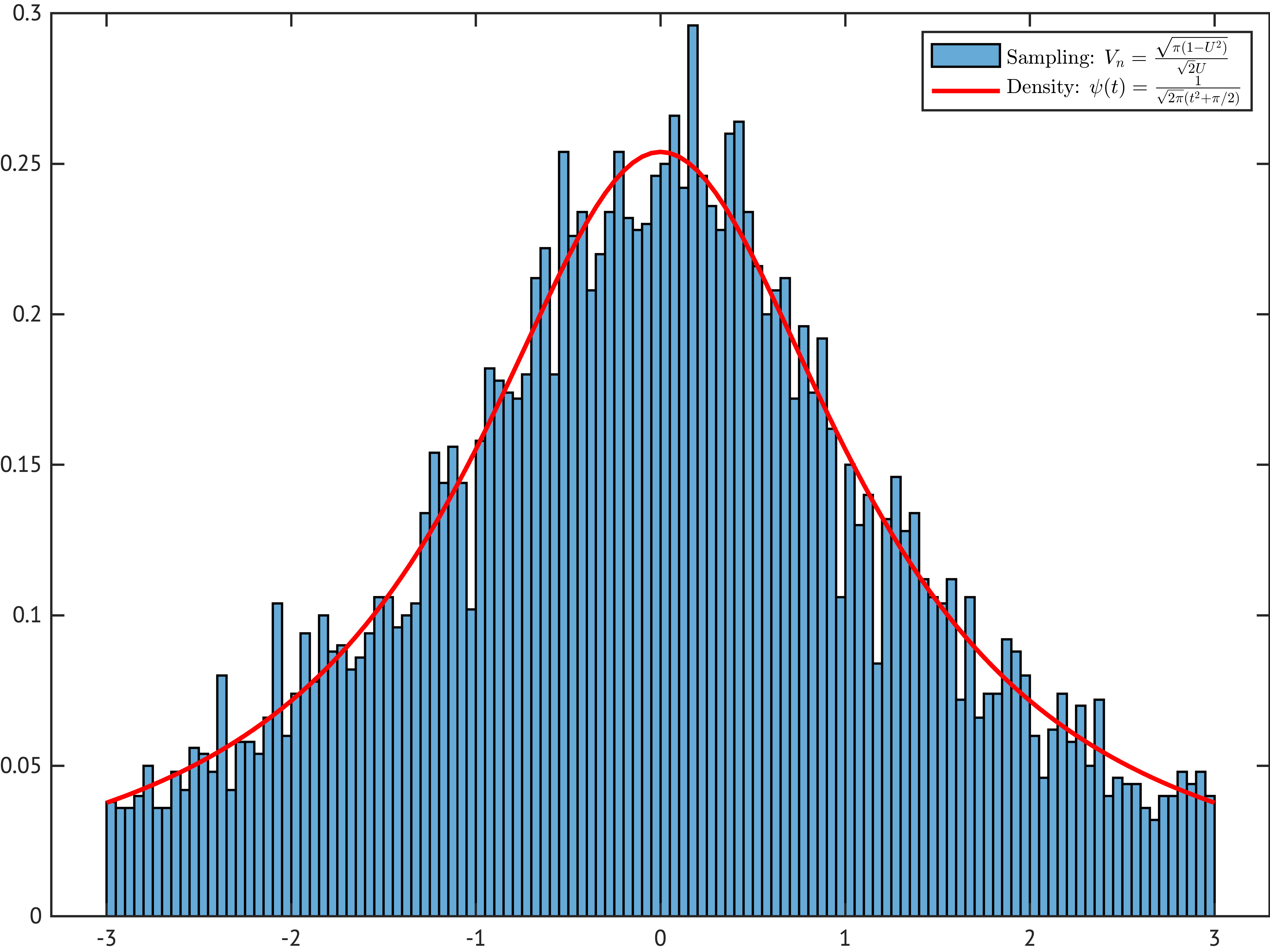
Figure 1. Cauchy distribution

4. Conclusion

The results in Theorem 2.2, Corollary 2.3 allow one to sample and simulate data when the parameter function $f$ is known. More interestingly, the inverse problem solved by 2.5 may be initiated to construct the “unknown” function $f$ in (2.2) which allows one to sample from a given particular distribution.

Some remarks to conclude our work are as follows: Among future perspectives for our work we may cite:

1. It is not hard to extend the results in Theorem 2.2 and Theorem 2.5 to random variables with several variables of the form

   $$V_{n}[f]=(f_{1}(U_{1})\sin(nU_{1}),\dots,f_{d}(U_{d})\sin(nU_{d}))$$

   where $f=(f_{1},\dots,f_{d})$, $U_{j}$ uniformly distributed in $(0,1)$ and $f_{j}\in L^{1}(0,1)$.

2. The condition ($\mathcal{L}$).1) may be relaxed as “$\psi$ of bounded variation in each $[a,b]\subset(0,\infty)$”. See [17].

3. A large class of functions satisfying ($\mathcal{L}$) is the set of even functions $\psi$ such that $\psi\in L^{1}(0,\infty)$ and $\psi(t)=\sqrt{t}\varphi(t)$ with $\varphi$ is in the Schwartz class $\mathcal{S}(0,\infty)$.

In a future work the following problems will be investigated.

1. Study the stability of the limiting law for the direct problem, respectively the stability of the parameter function $f$ for the inverse problem. That is:

   • If $f$ is replaced by a perturbed version $f_{\epsilon}$, how the limiting law is perturbed?

   • Respectively, if the density $\psi$ is replaced by a perturbed version $\psi_{\epsilon}$, how the parameter function $f$ is perturbed?

2. Looking for characterization results in Theorem 2.2 and Theorem 2.5.

References

- [1] M. Abramowitz and I. A. Stegun. Handbook of mathematical functions with formulas, graphs, and mathematical tables, volume 55. US Government printing office, 1948.
- [2] A. Addaim, D. Gretete, and A. A. Madi. Enhanced box-muller method for high quality gaussian random number generation. International Journal of Computing Science and Mathematics, 9(3):287–297, 2018.
- [3] F. Black and M. Scholes. The pricing of options and corporate liabilities. Journal of political economy, 81(3):637–654, 1973.
- [4] G. E. Box and M. E. Muller. A note on the generation of random normal deviates. The annals of mathematical statistics, 29(2):610–611, 1958.
- [5] M. Cardona and R. Merlin. Light scattering in solids IX. Springer, 2007.
- [6] W. Feller. An introduction to probability theory and its applications, Volume 2, volume 81. John Wiley & Sons, 1991.
- [7] B. E. Fristedt and L. F. Gray. A modern approach to probability theory. Springer Science & Business Media, 2013.
- [8] T. Hastie, R. Tibshirani, J. H. Friedman, and J. H. Friedman. The elements of statistical learning: data mining, inference, and prediction, volume 2. Springer, 2009.
- [9] D.-U. Lee, W. Luk, J. D. Villasenor, and P. Y. Cheung. A gaussian noise generator for hardware-based simulations. IEEE Transactions on Computers, 53(12):1523–1534, 2004.
- [10] D. G. Manolakis, V. K. Ingle, and S. Kogan. Statistical and Adaptive Signal Processing: Spectral Estimation, Signal Modeling, Adaptive Filtering and Array Processing. McGraw-Hill, 2000.
- [11] G. Marsaglia and W. W. Tsang. The ziggurat method for generating random variables. Journal of statistical software, 5:1–7, 2000.
- [12] D. C. Montgomery. Introduction to statistical quality control. John wiley & sons, 2019.
- [13] A. D. Poularikas. Transforms and applications handbook. CRC press, 2010.
- [14] C. Robert. Machine learning, a probabilistic perspective, 2014.
- [15] M. F. Schollmeyer and W. H. Tranter. Noise generators for the simulation of digital communication systems. ACM SIGSIM Simulation Digest, 21(3):264–275, 1991.
- [16] I. N. Sneddon. The use of integral transforms. New York: McGraw-Hill, 1972.
- [17] I. N. Sneddon. Fourier transforms. Courier Corporation, 1995.
- [18] N. M. Temme. Special functions: An introduction to the classical functions of mathematical physics. John Wiley & Sons, 2011.
- [19] D. B. Thomas, W. Luk, P. H. Leong, and J. D. Villasenor. Gaussian random number generators. ACM Computing Surveys (CSUR), 39(4):11–es, 2007.
- [20] R. Toral and A. Chakrabarti. Generation of gaussian distributed random numbers by using a numerical inversion method. Computer physics communications, 74(3):327–334, 1993.
- [21] D. E. Tyler. Robust statistics: Theory and methods, 2008.
- [22] G. N. Watson. A treatise on the theory of Bessel functions, volume 2. The University Press, 1922.