Stochastic comparisons of record values based on their relative aging
Abstract
In this paper we examine some relative orderings of upper and lower records. It is shown that if , the th upper record ages faster than the th upper record, where the data sets come from a sequence of independent and identically distributed observations from a continuous distribution. Sufficient conditions are also obtained to see whether the th upper record arisen from a continuous distribution ages faster in terms of the relative hazard rate than the th upper record arisen from another continuous distribution. It is also shown that the reversed hazard rate of the th lower record decreases faster than the reversed hazard rate of the th lower record, when . Preservation property of the relative reversed hazard rate order at lower record values is investigated. Several examples are presented to examine the results.
Key Words: Upper record values, Lower record values, Relative aging, Stochastic order.
1 Introduction
Order statistics result from a random sample of finite size, independent of the order of the observations in the sample. The extreme values of the sample are referred to as minimum order statistic and maximum order statistic. Record values are the extreme values of a sequence of random samples that converge to the extremes of the distribution under consideration. Formally, successive observations of a single random variable, called a sequence of random variables, yield two statistics, namely the upper record value and the lower record value. Extreme amounts of a random sequence of random variables are available as record values and, as a result, record values are important statistics that are useful to show the extremes of the distribution of observations. The record values have been extensively studied in the literature thus far. Because they are found in so many academic fields such as climatology, athletics, medicine, transportation, industry and so on, records are very popular. These records serve as time capsules. Through the history of records, we can examine how science and technology have developed and judge humanity based on historical achievements in a number of fields. Numerous long-term records have inspired the development of various mathematical models that reflect related record-keeping processes and predict future record outcomes. Records have been thoroughly studied in the literature. Considerable progress has been made in the field of stochastic orderings of record values. We cite the following sources for a selection of results: Khaledi [26], Hu and Zhuang [21], Raqab and Amin [39], Ahmadi and Arghami [3], Belzunce et al. [10], Kayid et al. [25], Esna-Ashari et al. [16], Aswin et al. [7] and references therein. Raqab and Asadi [40] have published more recent work on the mean residual lives of data sets considering reliability, aging aspects and other relevant properties. For more information on distribution theory and its applicability to different types of data modeled by record values, see Ahsanullah [2] and Arnold et al. [5].
Aging is a universal phenomenon that affects both mechanical systems and living beings. The age of a living organism is the time at which this organism is still alive and functioning. The aging process of an object is usually due to the wear and tear of the object. It usually explains how a system or living being gets better or worse as it gets older. In recent decades, researchers have been intensively studying stochastic aging. Numerous ideas on stochastic aging have been developed in the literature to characterize various aging features of a system, such as the increasing failure rate (IFR), the increasing failure rate average (IFRA), etc. There are three categories of aging: no aging, negative aging and positive aging. Two publications that provide a quick overview of different aging principles are Barlow and Proschan [8] and Lai and Xie [30]. Comparative aging is a useful idea that describes how one system ages relative to another and is similar to these other aging terms.
The term “relative aging” refers to the aging of one system compared to another. The commands for faster aging are those that compare the respective ages of the two systems. The relative age of two systems can be described by two additional sets of stochastic orders. The convex transformation order, the quantitative mean inactive time order, the star-shaped order, the superadditive order, the DMRL (decreasing mean residual life) order, the s-IFR order, and other so-called transformation orders belong to the first set of stochastic orders, which characterize whether one system ages faster than another in terms of increasing failure rate, increasing failure rate on average, new better than used, etc. Barlow and Proschan [8], Bartoszewicz [9], Deshpande and Kochar [14], Kochar and Wiens [28], Arriaza et al [4], Nanda et al [36] and the references therein provide a thorough treatment of these orderings. The monotonicity of the ratios of certain reliability measures, such as the mean residual life function, the inverted hazard rate function and the hazard rate function, defines the second group of stochastic orders, often referred to as faster aging orders. We recommend reading Kalashnikov and Rachev [22], Sengupta and Deshpande [42], Di Crescenzo [15], Finkelstein [17], Razaei et al. [41], Hazra and Nanda [19], Misra et al [34], Kayid et al [24] and Misra and Francis [35] for information on the foundations and applicability of these orders.
In reliability and survival analysis, the proportional hazard (PH) model, also known as Cox’s PH model (see Cox [13]), is often used to analyze failure time data. Later, other models were developed, including the proportional mean remaining life model, the proportional odds model, the proportional inverse hazard rate model, and others (see Marshall and Olkin [32], Lai and Xie [30], and Finkelstein [18]). The phenomenon of crossing hazards and, further, crossing mean residual lifetimes has been observed in numerous real-world scenarios (see Mantel and Stablein [31], Pocock et al. [38] and Champlin et al. [12]). Based on the idea of relative aging, Kalashnikov and Rachev [22] developed a stochastic ordering (called faster aging ordering in the hazard rate) to address this problem of crossing hazard rates. In fact, this strategy could be seen as a solid replacement for the PH model. Sengupta and Deshpande [42] give a thorough analysis of this order. They also presented two other related types of stochastic ordering.
Subsequently, Razaei et al. [41] offered a similar stochastic ordering in the form of the reversed hazard rate functions, while Finkelstein [17] proposed a stochastic ordering based on the mean residual life functions characterizing the relative ages of two life distributions. Hazra and Nanda [19] presented some generalized orderings in this direction.
However, the problem of the relative aging ordering of record values has not yet been considered in the literature. The aim of the present study is to initiate such an investigation in order to develop preservation properties of the relative hazard rate order and the relative reversed hazard rate order under upper records and lower records, respectively.
The structure of the paper is as follows. In Section 2, we introduce some preliminary concepts and definitions. In Section 3, we investigate the preservation property of the relative hazard rate order under upper records. In Section 4, preservation property of the relative reversed hazard rate order under lower records is investigated. In Section 5, we conclude the paper with further remarks and illustrations on current and future research.
2 Preliminaries
In this section, we bring some preliminaries that will be used throughout the paper. The definitions of the ageing faster orders utilized in our paper are provided below.
Definition 2.1.
Let and be two absolutely continuous random variables with hazard rate functions and , respectively, and reversed hazard rate functions and , respectively. It is then said that ages faster than in
-
(i)
hazard rate, denoted by , if
-
(ii)
reversed hazard rate, denoted by , if
Let us look at a technical system that experiences shocks like voltage peaks. A set of independent and identically distributed (i.i.d.) rvs with a common continuous cdf , pdf and survival function can then be used to simulate the shocks. The loads on the system at different points in time are represented by the shocks. The record statistics (values of the highest stresses reported so far) of this sequence are of interest to us. As we consider the lifetime of devices in our context, we thus suppose that the observations which produce record values are non-negative. Hence, the record values are consequently non-negative. The -th order statistics from the first observations are labeled with the symbol .
Next, we define the upper record values and upper record timings , respectively, as follows:
where
It is commonly known that the pdf and sf of represented by and respectively, are given by
| (1) |
and
| (2) |
where the last identity is derived by using the expansion of incomplete gamma function (see e.g. [6]). In contrast to the upper record values are the lower record values. The th lower record time with is stated as
and the -th lower record is enumerated as The pdf of can be acquired as
| (3) |
In addition, has cdf:
| (4) |
Three stochastic orders which consider magnitude of random variables rather than their relative aging behaviours are defined below according to Shaked and Shanthikumar [43].
Definition 2.2.
Let us suppose that and represent the lifetime of two devices. It is said that is smaller than in the
-
(i)
hazard rate order, denoted by , if
-
(ii)
reversed hazard rate order, denoted by , if
-
(iii)
usual stochastic order, denoted by , if
The following definition is regarding the aging property of a life unit.
Definition 2.3.
Let be a lifetime random variable with hazard rate and reversed hazard rate . It is said that has
-
(i)
increasing failure rate (denoted as ), if is increasing in .
-
(ii)
decreasing reversed hazard rate (denoted as ) if is decreasing in .
The following definition is due to Karlin [23] which be used frequently in the sequel.
Definition 2.4.
Let be a non-negative function. It is said that is Totally positive of order 2 () in where and are two arbitrary subsets of whenever
| (5) |
If the direction of the inequality given after determinant in (5) is reversed then it is said that is Reverse regular of order 2 () in .
3 Relative aging of upper record values
Suppose that and are two non-negative rvs with absolutely continuous cdfs and , and the associated pdfs and , respectively. We also denote by and the sfs of and , respectively. Let us obtain the expression of hazard rate of and , as the upper record values of two sequences of rvs and , respectively. From Eq. (1) and Eq. (2), the hazard rate of at point of time, is derived as
| (6) |
In a similar manner, the hazard rate of at time point , is derived as
| (7) |
Next, we present a result on the preservation property of relative hazard rate order under distribution of upper records.
Theorem 3.1.
Let and also let . Then, implies .
Proof.
We first prove that for every and for all . Then, we establish that . From transitivity property of the relative hazard rate order, one concludes that . For , let us denote
By using (3), one can then write
It suffices to show that increases in . One can get
Note that in increasing in , if and only if,
where for and , for and also . It is plain to see that is in and is also in . Thus, by using general composition theorem of Karlin [23], is in Hence, we established that for every .
Now, we prove that , for all From Eq. (3) and Eq. (7), one has the following
Since , thus is increasing in . Thus, it is sufficient to prove that
Now, we can write
where and is a discrete rv with pmf
Since thus is decreasing in Hence, from Lemma 2.1 of Khaledi et al. [27], is decreasing in . Therefore, since for every , , thus is increasing in . On the other hand, from assumption we have , and thus, for all , it holds that As a result, is an increasing function in , for every Further, it can be shown readily that is in , which further implies that for all . Now, by using Lemma 2.2(i) of Misra and van der Meulen [33], is increasing in . Now, the result is proved. ∎
Stochastic comparison of convolutions of exponential random variables has been an important subject of research in literature (see, e.g., Bon and Pãltãnea [11] and Kochar and Ma [29]). However, relative ordering of convolutions of exponential random variables has not been investigated in literature thus far. In the next example, we make the relative hazard rate ordering of convolutions of i.i.d. exponential random variables according to the relative hazard rate order. Note that a non-negative rv is said to have Erlang distribution with parameters whenever it has pdf for all , where and .
Example 3.1.
Let us suppose that and are two i.i.d. sequences of exponential random variables with means and , respectively, such that . From Eq. (1), and have pdfs
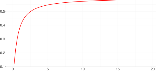
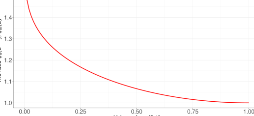
which are the pdfs of two Erlang distributions with parameters and respectively. On the other hand, it is a well-known fact that partial sums of i.i.d. exponential random variables and follow Erlang distribution with parameters and , respectively. Therefore, and are equal in distribution with and , respectively. From Eq. (3) and Eq. (7), one gets
Since , thus . Thus, for every , by using Theorem 3.1, one concludes that In Figure 1, we have plotted the hazard rate ratio of convolutions of exponential random variables, which is an increasing function.
In Theorem 3.1 there is an order condition that , However, this is a strong condition that may not be satisfied. In the residual part of this section, we want to relax the condition to obtain the preservation property of the relative hazard rate order under upper records. The following lemma is useful to prove such result.
Lemma 3.1.
Let for . Then, is a non-negative increasing function of for every .
Proof.
Let us suppose that is a discrete random variable with the following probability mass function
Then, one has the following
where is a decreasing function of and it is an increasing function of . Note that is an function in . Hence, for every , i.e., is stochastically decreasing in . Thus, by using Lemma 2.2(i) of Misra and van der Meulen [33], is an increasing function of . This completes the proof of lemma. ∎
The limiting behaviour of hazard rates ratio is an important problem in reliability analysis (see, e.g., Navarro and Sarabia [37]). Let us define
In what follows, we assume that and are positive and finite. The following theorem is the main result of this section.
Theorem 3.2.
Let where for . If then, implies
Proof.
From Eq. (3) and Eq. (7), for all one has the following
Thus, it is evident that
Since from assumption thus it is enough to show that is increasing in , or equivalently demonstrate that
| (8) |
We have
Note that since is increasing in , thus , for all and , for all which further imply that for all and that for all respectively. The second implication is due to the recursive formulas and so that if for all , then one concludes for all Now, one has the following
Remark 3.1.
It is to be mentioned that the result of Theorem 3.2 in situations where and are equal in distribution, could also be achieved by using Theorem 3.1, since the assumption is satisfied when and have a common distribution. It is remarkable in the context of Theorem 3.2, that if and are equal in distribution, then . Note that is increasing in , if and only if for every ,
The above inequality is also equivalent to
which means that is increasing in We can write
in which is increasing in , if and only if,
where for and for , and . Since is in and is also in thus the required result follows from general composition theorem of Karlin [23]. Now, since as discussed before, thus for every where one has
where the last inequality holds because for every Therefore, from Theorem 3.2, we deduced that if then .
The following example presents an example where Theorem 3.2 is applicable. However, we can not deduce the result using Theorem 3.1 because .
Example 3.2.
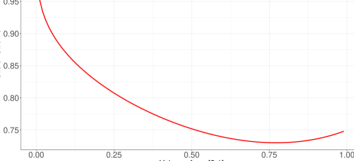
Let us consider and as two random lifetimes with Lomax distributions having sfs and The hr functions of and are then calculated as and , which yields The function is increasing in . Thus, according to definition, . It is seen that and . It is trivial that, for all , which means , and consequently, . Therefore, the condition of Theorem 3.1 does not hold. We want to compare the second upper record from a sequence of i.i.d. random lifetimes adopted from to the third upper record from a sequence of i.i.d. random lifetimes following . Hence, and . We show using the setting of Theorem 3.2 that For , we observe that
from which one further obtains
After some routine calculation, we derive
and, similarly,
Therefore,
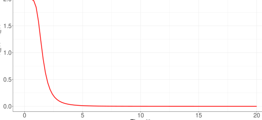
It can be checked using website https://www.dcode.fr/maximum-function that . One can also see Figure 2. Hence, the condition of Theorem 3.2 is satisfied and hence the required result follows.
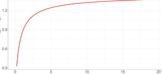
In Example 3.2, one can further obtain
and
In Figure 3 we plot the graph of to exhibit that it is an increasing function in .
4 Relative comparison of lower record values
In this section, we consider the lower records and from two sequences of rvs and , each containing i.i.d. observations. The rhr of is obtained as
| (9) |
Analogously, the rhr of at time point , is acquired as
| (10) |
Next, we present a result on the preservation property of relative reversed hazard rate order under distribution of lower records.
Theorem 4.1.
Let and . Then, yields .
Proof.
Firstly, we demonstrate that holds true for and for every such that . Then, it will be proved that . Due to the transitivity property of the relative reversed hazard rate order, it is deduced that . Keeping the notations of Theorem 3.1 in mind, and in view of (4), we can write
In the proof of Theorem 3.1, it was shown that in increasing in . Hence, since is decreasing in , thus is decreasing in . Therefore, for every . To finalize the proof, we need to prove , for every In the spirit of Eq. (4) and Eq. (10), we get
Following assumption, we have . Hence is decreasing in . It thus suffices to establish that
Let us write
where and is an rv with pmf
Since thus from Hazra and Misra [20], is increasing in . Thus, is decreasing in . From assumption, it holds that , and as a result, for all , Therefore, is increasing in , for all It can be seen readily that is in , which in turn yields for all . On applying Lemma 2.2(ii) of Misra and van der Meulen [33], is decreasing in . Now, the result is proved. ∎
The following example presents a situation where Theorem 4.1 is applicable.
Example 4.1.
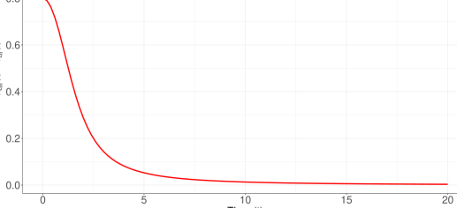
We suppose that and have inverse Weibull distribution with cdfs and where We can get and Since thus . It is also trivial to see that . Let us choose and . The result of Theorem 4.1 implies that One has the following
In Figure 4 we plot the graph of and it is shown that this function decreases in which validates the result of Theorem 4.1.
The extremal behaviour of reversed hazard rates ratio is considered here. Let us define
In the sequel, we assume that and are positive and finite. In the following theorem the condition of in Theorem 4.1 is relaxed.
Theorem 4.2.
If then, implies
Proof.
In view of Eq. (4) and Eq. (10), for all we get
Therefore,
By assumption we have which means is decreasing. Thus, we only need to show that is decreasing in , or equivalently, we can prove that
| (11) |
One has
Since is decreasing in , thus , for all and , for all Hence, for all and also for all where the second inequality follows from the identities and . This is because if for all , then for all Therefore,
where the first inequality holds because for all and the last inequality is due to for all and since by Lemma 3.1, is increasing in It is now realized that (11) is fulfilled if for all . We know that is a non-negative function, and further, it is trivial that thus the recent inequality holds if, and only if,
∎
It is remarkable here that when and are equal in distribution then, and further . In the spirit of Remark 3.1, since is increasing in for every and because , thus for every one observes that
Hence, using Theorem 4.1, one obtains This result could also be concluded by applying Theorem 3.2.
The next example illustrates a situation where Theorem 4.1 is not applicable while the result of Theorem 4.2 works.
Example 4.2.
Let and be two random lifetimes with Inverse Weibull distributions having cdfs and The rhr functions of and are obtained as and , which further implies that The function is, therefore, non-increasing in . By definition, . We can see that . For all , i.e., and moreover . This means that the condition of Theorem 4.1 is not satisfied. Here, we take and . By using Theorem 4.2 we shall conclude that For , in the sprit of the proof of Theorem 3.2 in Example 3.2, one gets
We can check using website https://www.dcode.fr/maximum-function that as is shown in Figure 5. The condition of Theorem 4.2 holds and the result follows.
In Example 4.2, we can obtain the rhr functions of and as follows:
and
In Figure 6 we have plotted the graph of to exhibit that it decreases in .
5 Conclusion
In this paper, we first presented conditions under which the relative hazard rate order between and with the respective distributions and is translated into the relative hazard rate order of the upper record values and resulting from sequences of random lifetimes following the base distributions and . The first result states that if and , then implies , which means that if ages faster than in terms of the hazard rate function, then ages correspondingly faster than . In situations where and have an IFR distribution, means that the hazard rate function of increases faster than the hazard rate function of . It is also concluded that if then . It has been shown that is not a necessary condition to obtain the preservation property of order under upper record values. We have secondly given conditions under which the relative reversed hazard rate order between and is translated into the relative reversed hazard rate order of lower record values and . We have shown that if and , then results in . If then and have a DRHR distribution, then is equivalent to saying that the reversed hazard rate function of decreases faster than the reversed hazard rate function of . In this context, if then . We have also proved that is not a necessary condition to obtain the preservation property of order under lower record values.
The results obtained in this study can be used to describe further findings on record values. The hazard rate function and reversed hazard rate function of a lifetime random variable are proportional to the probabilities and respectively, where is a very small positive number. Usually it is important to predict future upper or lower records. Therefore, it is a natural question whether a record higher than will be reached directly after . Let us assume and have the cdfs and respectively. For example,
indicates that if the th upper record from the sequence of i.i.d. lifetimes from (i.e., ) has not retained until time and also if the th upper record from the sequence of i.i.d. lifetimes from (i.e., ) has not retained until time , then it is more likely in the time in comparison with the time that is equal to a value in a small neighborhood after than that to be equal to such value in a small neighborhood after . Moreover, there is another question whether a lower record less than has retained right before . We observe that
which shows that if the th lower record from the sequence of i.i.d. lifetimes from (i.e., ) has retained until time and further if the th lower record from the sequence of i.i.d. lifetimes from (i.e., ) has also retained before time , then it is more likely in the time compared with the time that is equal to a value in a small neighborhood before than that to be equal to such value in a small neighborhood before .
In future research, one may consider simplifying the condition of Theorem 3.2 with respect to and and also simplifying the condition of Theorem 4.2 on the basis of and . The existence of the supremum in Theorem 3.2 was guaranteed in Remark 3.1 for the case that and are equally distributed, where and also after the proof of Theorem 4.2 it was guaranteed that the supremum exists in the cases where and have a common distribution leading to . However, as explained in Example 3.2 and Example 4.2, there are also more complicated situations in which the suprema exists. Further implications of the relative ordering of dataset values, e.g. finding bounds for the survival functions of the upper datasets and the distribution function of the lower datasets, can also be considered in the future.
Acknowledgments
This work was supported by Researchers Supporting Project number (RSP2024R392), King Saud University, Riyadh, Saudi Arabia.
Conflict of interest
On behalf of all authors, the corresponding author states that there is no conflict of interest.
References
- [1] Abouammoh, A. R. and Qamber, I. S. (2003). New better than renewal-used classes of life distributions. IEEE Transactions on Reliability 52(2), 150–153.
- [2] Ahsanullah, M. (1995). Record Statistics. New York: Nova Science Publishers.
- [3] Ahmadi, J., Arghami, N. R. (2001). Some univariate stochastic orders on record values. Communications in Statistics-Theory and Methods 30, 69-78.
- [4] Arriaza, A., Sordo, M.A. and Suárez-Liorens, A. (2017). Comparing residual lives and inactivity times by transform stochastic orders. IEEE Transactions on Reliability 66, 366– 372.
- [5] Arnold, B. C., Balakrishnan, N., Nagaraja, H. N. (1998). Records. New York: John Wiley.
- [6] Arnold, B. C., Balakrishnan, N. and Nagaraja, H. N. (2008). A first course in order statistics, volume 54 of Classics in Applied Mathematics.
- [7] Aswin, I. C., Sankaran, P. G. and Sunoj, S. M. (2023). Some reliability aspects of record values using quantile functions. Communications in Statistics-Theory and Methods 1-21.
- [8] Barlow, R. E. and Proschan, F. (1975). Statistical theory of reliability and life testing. New York: Holt, Rinehart and Winston.
- [9] Bartoszewicz, J. (1985). Dispersive ordering and monotone failure rate distributions. Advances in Applied Probability 17, 472–474.
- [10] Belzunce, F., Lillo, R. E., Ruiz, J. M., Shaked, M. (2001). Stochastic comparisons of nonhomogeneous processes. Probability in the Engineering and Informational Sciences 15, 199–224.
- [11] Bon, J. L. and Pãltãnea, E. (1999). Ordering properties of convolutions of exponential random variables. Lifetime Data Analysis 5, 185–192.
- [12] Champlin, R., Mitsuyasu, R., Elashoff, R. and Gale, R.P. (1983). Recent advances in bone marrow transplantation. In: UCLA Symposia on Molecular and Cellular Biology, ed. R.P. Gale, New York 7, 141–158.
- [13] Cox, D. R. (1972). Regression models and life-tables. Journal of the Royal Statistical Society, Series B 34, 187–220.
- [14] Deshpande, J. V. and Kochar, S. C. (1983). Dispersive ordering is the same as tail-ordering. Advances in Applied Probability 15, 686–687.
- [15] Di Crescenzo, A. (2000). Some results on the proportional reversed hazards model. Statistics and Probability Letters 50, 313–321.
- [16] Esna-Ashari, M., Balakrishnan, N. and Alimohammadi, M. (2023). HR and RHR orderings of generalized order statistics. Metrika 86(1), 131–148.
- [17] Finkelstein, M. (2006). On relative ordering of mean residual lifetime functions. Statistics and Probability Letters 76, 939–944.
- [18] Finkelstein M. (2008). Failure rate modeling for reliability and risk. London, Springer.
- [19] Hazra, N. K. and Nanda, A. K. (2016). On some generalized orderings: In the spirit of relative ageing. Communications in Statistics-Theory and Methods 45, 6165–6181.
- [20] Hazra, N. K. and Misra, N. (2021). On relative aging comparisons of coherent systems with identically distributed components. Probability in the Engineering and Informational Sciences 35, 481–495.
- [21] Hu, T., Zhuang, W. (2006). Stochastic orderings between p-spacings of generalized order statistics from two samples. Probability in the Engineering and Informational Sciences 20, 465–479.
- [22] Kalashnikov, V. V. and Rachev, S. T. (1986). Characterization of queueing models and their stability. In: Probability Theory and Mathematical Statistics, eds. Yu. K. Prohorov et al., VNU Science Press, Amsterdam 2, 37-53.
- [23] Karlin, S. Total Positivity, Stanford University Press, 1968.
- [24] Kayid, M., Izadkhah, S. and Zuo, M. J. (2017). Some results on the relative ordering of two frailty models. Statistical Papers 58, 287–301.
- [25] Kayid, M., Alrubian, A. and Abouammoh, A. (2021). Stochastic analysis of an age-dependent mixture truncation model. Naval Research Logistics 68, 963–972.
- [26] Khaledi, B.-E. (2005). Some new results on stochastic orderings between generalized order statistics. Journal of the Iranian Statistical Society 4, 35-49.
- [27] Khaledi, B. E., Amiripour, F., Hu, T. and Shojaei, S. R. (2009). Some new results on stochastic comparisons of record values. Communications in Statistics-Theory and Methods 38, 2056–2066.
- [28] Kochar, S. C. and Wiens, D. P. (1987). Partial orderings of life distributions with respect to their ageing properties. Naval Research Logistics 34, 823–829.
- [29] Kochar, S. and Ma, C. (1999). Dispersive ordering of convolutions of exponential random variables. Statistics and Probability Letters 43, 321–324.
- [30] Lai, C. and Xie, M. (2006). Stochastic ageing and dependence for reliability. New York: Springer.
- [31] Mantel, N. and Stablein, D. M. (1988). The crossing hazard function problem. Journal of the Royal Statistical Society, Series D 37, 59-64.
- [32] Marshall, A. W. and Olkin, I. (2007). Life Distributions. Springer, New York.
- [33] Misra, N. and van der Meulen, E. C. (2003). On stochastic properties of m-spacings. Journal of Statistical Planning and Inference 115, 683–697.
- [34] Misra, N., Francis, J. and Naqvi, S. (2017). Some sufficient conditions for relative aging of life distributions. Probability in the Engineering and Informational Sciences 31, 83-99.
- [35] Misra, N. and Francis, J. (2018). Relative aging of -out-of- systems based on cumulative hazard and cumulative reversed hazard functions. Naval Research Logistics 65, 566–575.
- [36] Nanda, A. K., Hazra, N. K., Al-Mutairi, D. K. and Ghitany, M. E. (2017). On some generalized ageing orderings. Communications in Statistics-Theory and Methods 46, 5273–5291.
- [37] Navarro, J. and Sarabia, J. M. (2024). A note on the limiting behaviour of hazard rate functions of generalized mixtures. Journal of Computational and Applied Mathematics 435, 114653.
- [38] Pocock, S. J., Gore, S. M. and Keer, G. R. (1982). Long-term survival analysis: the curability of breast cancer. Statistics in Medicine 1, 93–104.
- [39] Raqab, M. Z., Amin, W. A. (1996). Some ordering results on order statistics and record values. IAPQR Transactions, Journal of the Indian Association for Productivity, Quality and Reliability 21, 1-8.
- [40] Raqab, M. Z., Asadi, M. (2008). On the mean residual life of records. Journal of Statistical Planning and Inference 138, 3660–3666.
- [41] Rezaei, M., Gholizadeh, B. and Izadkhah, S. (2015). On relative reversed hazard rate order. Communications in Statistics-Theory and Methods 44, 300–308.
- [42] Sengupta, D. and Deshpande, J. V. (1994). Some results on the relative ageing of two life distributions. Journal of Applied Probability 31, 991–1003.
- [43] Shaked, M. and Shanthikumar, J. G. (Eds.). (2007). Stochastic orders. New York, NY: Springer New York.