Causal Learning in Biomedical Applications

Abstract

We present a benchmark for methods in causal learning. Specifically, we consider training a rich class of causal models from time-series data, and we suggest the use of the Krebs cycle and models of metabolism more broadly.

1 Introduction

Understanding causal models is important in a number of fields, from healthcare to economics, as it allows for precise forecasting a training of reinforcement learning. Learning causal models involves extracting potential non-linear relationships and dependencies between variables from sampled time-series. For example, modelling of biomarkers of non-communicable disase as a function of diet and action monitoring has shown the potential of being a powerful tool to guide the recommendations on healthy diet.

We aim to learn causal models that extend basic causal models in several directions, which are relevant in biomedical appliations. In particular, such causal models need to handle nonlinear causality, such as the competition among bacterial strains for metabolites. Likewise, one may consider constraints that become active beyond certain thresholds. Dealing with latent variables, such as hormone concentrations, is a challenge that demands a balance between model complexity and interpretability. These models should also consider cyclic relationships, time-series dynamics, and mixture-model aspects, accommodating individual variations in metabolism without predefined subgroups.

2 Preliminaries and Related Work

Learning most causal models involves solving NP-Hard non-convex optimization problems. Just as there is “one” convex optimization and “many” non-convex optimization problems, there are many causal models and methods for learning them. Perhaps the most elegant approach to causal learning utilizes techniques from system identification.

System Identification and Linear Dynamic Systems (LDS)

Let $m$ be the hidden state dimension and $n$ be the observational dimension. A linear dynamic system (LDS) $\mathbf{L}$ is defined as a quadruple $(\mathbf{F},\mathbf{G},\mathbf{\Sigma},\mathbf{V})$, where $\mathbf{F}$ and $\mathbf{G}$ are system matrices of dimension $m\times m$ and $n\times m$, respectively. $\mathbf{\Sigma}\in\mathbb{R}^{m\times m}$ and $\mathbf{V}\in\mathbb{R}^{m\times m}$ are covariance matrices [30]. A single realization of the LDS of length $T$, denoted $\mathbf{X}=\{x_{1},x_{2},\ldots,x_{T}\}\in\mathbb{R}^{n\times s\times T}$ is defined by initial conditions $\phi_{0}$, and realization of noises $\upsilon_{t}$ and $\omega_{t}$ as

$$\phi_{t} =\mathbf{F}\phi_{t-1}+\omega_{t},$$ (1)

$$x_{t} =\mathbf{G}^{\prime}\phi_{t}+\upsilon_{t},$$ (2)

where $\phi_{t}\in\mathbb{R}^{m\times s}$ is the vector autoregressive processes with hidden components and $\left\{\omega_{t},\upsilon_{t}\right\}_{t\in\{1,2,\ldots,T\}}$ are normally distributed process and observation noises with zero mean and covariance of $\mathbf{\Sigma}$ and $\mathbf{V}$ respectively, i.e., $\omega_{t}\sim N(0,\mathbf{\Sigma})\in\mathbb{R}^{m\times s}$ and $\upsilon_{t}\sim N(0,\mathbf{V})\in\mathbb{R}^{n\times s}$. The transpose of $\mathbf{G}$ is denoted as $\mathbf{G}^{\prime}$. Vector $x_{t}\in\mathbb{R}^{n\times s}$ is the observed output of the system. In non-linear dynamical systems, one replaces the multiplication $\mathbf{F}\phi_{t-1}$ with a function $f(\phi_{t-1})$. It is well known [31] that there are multiple, equivalent conditions for the identifiability of $\mathbf{F},\mathbf{G}$, given by so-called Hankel matrices, conditions on the transfer function, or frequency-domain conditions, among others. The is also a recent understanding [28] of sample complexity of the problem.

Linear Additive Noise Models

Throughout causal modelling, one wishes to learn a function $f$, which is known as the structural assignment map, and is closely related to the $f$ above. Under the assumption that the structural assignments are linear, noises $N_{j},j=1,\dots,N$ are indepenedntly identically distributed (i.i.d.) and follow the same Gaussian distribution, or alternatively, noises $N_{j},j=1,\dots,N$ are jointly independent, non-Gaussian with strictly positive density, one obtains linear additive noise models (ANM). In studying ANM, one may benefit from a long tradition of work on linear system identification. In particular, the identifiability of linear ANM can be reduced to identifiability of linear dynamical systems (cf. Proposition 7.5 & Theorem 7.6 in [25]).

Bayesian networks

Another classic example in causal learning are Bayesian networks, first introduced by Pearl in 1985 [23]. Bayesian networks are formed by a directed acyclic graph (DAG), where each vertex $j$ represents a variable $X_{j}$, with edges going from one variable to another represent causal relationships. It is assumed that each variable $X_{j}$ is independent of other variables but for its parents ${PA}_{j}$ in the DAG, thus allowing a compressed representation of the joint probability as

$$P(X_{1},X_{2},\ldots,X_{N})=\prod_{j=1}^{N}P(X_{j}\mid\mathbf{PA}_{j}).$$ (3)

The most common approach to exact inference in Bayesian networks is the variable elimination algorithm [24]. Approximate inference algorithms are also often applied. The most common one is the Markov Chain Monte-Carlo (MCMC) algorithm that repeatedly samples from each variable conditioned on the values of its parents. The MCMC algorithm predates Bayesian networks and is often referred to as Gibbs sampling.

In relation to temporal data, the Dynamic Bayesian Networks (DBN) are a well-known extension [7, 17]. DBNs are defined by two Bayesian networks. The first defines the initial state, and the second is the transition model between $t$ and $t+1$, where nodes in layer $t$ are assumed to be independent. The network can then be unrolled into length $T$ so that each of the time slices for $t\geq 1$ is defined by the transition model.

Counterfactual Framework

The counterfactual framework can be used to derive causality. This approach focuses on the question of which input variable needs to change in order to change the output of a model. The counterfactual framework is connected with the calculation of interventions, i.e., assessing the change of output variables after a hypothetical change of an input variable. In counterfactuals, we ask which inputs need to change to observe a change in the output, while in intervention, we change the inputs to see the change in the output. The counterfactuals were introduced into Bayesian networks by Pearl [19]. Nowadays, their usage is broad, and they find usage in explainable machine learning models [16].

Granger Causality

The goal of the Granger Causality [9] is to detect a causal effect of a time series on another time series. The Granger causality measures correlations between the effect series and shifted cause series, thus detecting a lag that represents the time needed for the cause to take shape. The method uses various statistical tests to detect whether adding a cause into a predictive model significantly improves the prediction capabilities of the model. The original paper [9] used linear regression as the testing predictor. Further modifications of the original paper followed and included non-linearity [32], learning from multiple time series [4], applications on spectral data, i.e., in the frequency domain [11], model-free modifications [6], and nonstationarity [27].

Instrumental Variables

Instrumental variables can be used to infer causal effects when we cannot control the experimental setting. Suppose that we want to assess the causal effect of the explanatory variable $E$ on the dependent variable $D$. Normally, we would try to do statistical tests on whether variable $D$ changes when $E$ changes. However, in many applications in medicine, economics, and others, this is not possible, as both $E$ and $D$ can have a common cause and be, therefore, correlated. This introduces bias in many statistical tests. To overcome the issue, we include a third variable, instrument variable $I$, which we can control and which has influence on $D$ only through $E$. Then, we observe changes of $D$ on $I$. When the applied predictor is linear regression, the predictor is a special case of a linear dynamic system [29]. The existence of a hidden state then allows the removal of the correlations stemming from a common, unobserved cause [29].

Instrumental variables are, however, concepts that can be used well beyond linear regression. Non-linear [20] and non-smooth [3] modifications exist. Sometimes, there is a requirement that instrumental variables might have common cofounders. This multilevel modeling is implemented in the instrumental variable toolkit by [13]. Similarly, [8] allow for a latent (hidden) variable.

Tractable Probabilistic Models

The tractable probabilistic models (TPMs) are a large group of methods that can be used to model probabilistic distributions compactly, in the spirit of neural networks approximating functions. A prime example of TPMs are sum-product networks (SPNs) [26], which represent the probability distribution as a DAG, where “input” random variables are assigned to leaves. Each non-leaf node corresponds to one of two operations, either sum or product. The weights of the edges are then used to learn the probability distribution. The original paper [26] also proposed an algorithm to learn the structure using a backpropagation and expectation maximization. The SPNs are only a subgroup in the broad class of probabilistic circuits [5]. The unified formalism allows to use different type of nodes besides the sum and product nodes. Dynamic versions [15, e.g.] are able to work with temporal data.

See also Table 1 in the next section for an overview.

3 The Challenge

As suggested in the Introduction, we would like to learn causal models that are more expressive than many traditional models. In our view, expressivity of the causal model entails:

• quantitative aspects of causality, also in order to simulate from the causal model

• non-linear aspects of causality

• hidden states (latent variables) of an a priori unknown dimension.

• At the same time, one would like to preserve as much explainability as possible, perhaps through targeted reduction [12].

• cycles in causal relationships

• time-series aspects, such as nonanticipativity and delays: clearly, causal relationships should be established between the cause in the past and the effect in the future, with some delay between the two.

• mixture-model aspects: clearly, there are variations between the metabolism in various individuals, perhaps due to genomic differences. One should explore joint problems [21], where multiple causal models are learned without the assignment of individuals to subgroups represented by the causal models given a priori.

Ability to simulate from the model entails:

• quantitative aspects of causality, in order to simulate from the causal model

• time required to simulate from the model scaling modestly (with the the number of random variables and numbers of samples).

Ability to learn the model entails:

• sample complexity: number of samples required to build the model. Even simple models such as HMM comprise learning Gaussian mixture models, which are known to have high sample complexity.

• time complexity: time required to learn the model. Again, even HMM are [2, 14] cryptographically hard to learn in the setting where one has access to i.i.d. samples of observation sequences.

Tool	Quantitative	Non-linear	Hidden st.	Cycles	Temporal	Mixture-models	Multiple trajectories	Structure learning in $\mathcal{P}$	Likelihood calculation in $\mathcal{P}$	Marginalization in $\mathcal{P}$	Simulation from the model
Casual Bayesian networks	✓	✓	✓	✗	✓	✓	✓	✗	✓	✗	✓
Structural Equation Modeling	✓	✓	✓	✓	✓	✓	✓	✗	-	-	-
Counterfactual Framework	✓	✓	✓	✓	✓	✓	✓	✗	-	-	-
Granger Causality	✓	✓	✗	✗	✓	✗	✓	✓	-	-	-
Bayesian Structural Time Series Models	✓	✓	✓	✓	✓	✓	✓	✗	-	-	-
Instrumental Variables	✓	✓	✓	✗	✓	✓	✓	✗	-	-	-
Tractable Probabilistic Models	✓	✗	✗	✗	✓	✓	✓	✗	(✓)	(✓)	(✓)

Table 1: Summary of features of selected methods and frameworks.

Let us discuss some of these in more detail.

Cycles

Standard Bayesian networks do not normally support cycles between the variables. The causal relationships need to form a directed acyclic graph (DAG). Likewise, Granger causality does not support cyclic dependencies by definition. The Granger causality aims to find out whether one variable can be helpful in predicting the future of a second variable. As a result, we are detecting some time lag, that the second variable correlated with the first variable shifted to the future. To obtain a cyclic relationship, we would need a sequence of positive time lags that sum together to zero, which is not possible.

Under some circumstances, we can model cyclical relationships with Dynamic Bayesian networks (DBNs). For each variable, we have its realizations for time $t=1,2,\ldots,T$. As a result, DBNs can then be used to model situations, such as the one when $X_{t}$ causes $Y_{t+1}$, $Y_{t+1}$ causes $Z_{t+2}$, which in turn causes $X_{t+3}$. The overall graph is still a DAG, as there cannot be a cycle within a one-time slice, and neither can a variable have an effect on the past.

Hidden state and Mixture-models

Modeling a hidden state in the model and sampling from the mixture of models are tightly connected, as the second can be reduced to the first. Suppose that we want to model a mixture of two distributions. We can build two separate models for each of the distributions. Then, we introduce a hidden state that models a binary decision, whether we sample from the first or the second distribution.

Model learning

When we are interested in the time complexity of model learning, the time requirements differ based on the techniques used. The Bayesian networks do not generally have exact polynomial-time learning. In Granger causality, the complexity of mining causal relationships depends on the algorithms and methods used. In the simplest scenarios, we can base the causal relationships on the F-test, which can be calculated in linear time, assuming that the cumulative distribution function of the Fisher–Snedecor distribution (F-distribution) is precomputed.

Non-linear dependencies

In many cases, the possibility of having non-linear models is part of extensions of the original methods. A prominent example of such a method is Granger’s causality. The original method was developed with linear dependencies between the features. But further extensions were developed to include nonlinearities, for example, [32]. In Bayesian networks, the original version [23] considered only propositional variables, but subsequent versions [10, e.g.] considered also continuous variables and non-linear dependencies.

4 The Benchmark

As the causal learning community matures, one would like to learn models that are more expressive (see above) and to learn them from datasets that go beyond toy examples.

In this paper, we present a simulated dataset based on the Krebs cycle. The Krebs cycle, also known as the citric acid cycle, is one of the fundamental pathways of biochemistry. The cycle, as illustrated in Figure 1, allows organisms that breathe to convert energy stored in food to a key energy source (ATP) in muscle cells, for example. Such a cycle presents a natural example of time series that can be used to infer causal relationships between concentrations of the reactants.

Figure 1: Illustration of the Kreb’s cycle reactions used to similate the concentrations.

4.1 The Data

Depending on the modelling of the time series, each of the reactions can be represented by one or more causal relationships. Our benchmark is based on a simulator the GitHub repository at [18]. The simulator creates a virtual box with desired particles. The particles move inside the box, following the Boltzmann distribution. Once particles get close to each other, a pre-defined list of reactions is scanned to determine whether a reaction occurs, and if so, reactants are replaced with a product. The simulation then continues, and concentrations of different particles are then used as test time series. As a result, the time series contains noise (caused by the random location of particles), which is added to the locally linear behavior of the system.

In this a way, we have generated four datasets, consisting of a time series with $5$ to $5000$ time steps and $16$ features for the reactants, including $10$ in the main cycle and $6$ additional ones (incl. water). Each of the following datasets is based on simulating approximately $2500$ molecules in the bounding box:

• contains $100$ series with normally distributed prior distributions and absolute concentrations.

• contains $120$ series with relative concentrations, where for each triplet of the $10$ main cycle reactants, we used uniform priors, and the remaining $7$ particles were set to zero. Such a distribution is motivated by allowing the tested approaches to trace how the higher concentration of the three selected compounds moves forward in the cycle.

• focuses on learning from few long time series. In this case, we have $10$ series with $5000$ time steps. We use

• considers $10000$ time series with only $5$ time steps each, a complementary scenario to KrebsL.

The datasets are summarized in Table 2, showing the dimensions of the time series, the number of molecules used in the simulation, as well as other important features of the data.

Dataset	N. features	Lenght	N. series	Initialization	Concentrations
KrebsN	$16$	$500$	$100$	Normal distribution	Absolute
Krebs3	$16$	$500$	$120$	Excitation of three	Relative
KrebsL	$16$	$5000$	$10$	Normal distribution	Absolute
KrebsS	$16$	$5$	$10000$	Normal distribution	Absolute

Table 2: Summary of the datasets in the Krebs cycle.

4.2 Evaluation Criteria

The performance of supervised machine learning methods are compared based on K-fold cross validation and F-Beta Score (or F1-score). K-Fold Cross-Validation is a technique used to assess the performance and generalizability of a machine learning model. It involves dividing the dataset into $k$ equally sized folds, training the model on $k-1$ folds, and validating it on the remaining fold. This process is repeated $k$ times, with each fold serving as the validation set once. The final performance metric is the average of the metrics obtained in each iteration.

The precision, recall, and $F_{1}$ score, which have been widely used in casual model performance measurements, are defined as

$$F_{1}=2\cdot\frac{\textrm{precision}\cdot\textrm{recall}}{\textrm{precision}+\textrm{recall}},$$ (4)

$$\textrm{precision}=\frac{TP}{TP+FP},$$ (5)

$$\textrm{recall}=\frac{TP}{TP+FN},$$ (6)

where $TP$, $FP$, and $FN$ are the numbers of true positives, false positives, and false negatives, respectively.

In the case of deterministic methods, the stability of the F1-score cannot be evaluated by simple repeated evaluations followed by standard deviation calculation. Therefore, we recommend using an approach similar to cross-validation to show the stability of the results. In each evaluation, instead of plain restart, we can keep $10\,\%$ of the dataset aside to randomize data instead of the method. As a result, by doing repeated evaluations, it is possible to obtain the results’ standard deviations and confidence intervals.

4.3 A Baseline

To illustrate the dataset, we include results of the DyNoTears [22], a state-of-the-art method for causal discovery, implemented in the CausalNex [1] package. DyNoTears is provided with information that forbids edges within the same time slice, and the regularization parameter $\lambda_{a}$ is selected from the list $10^{-6},10^{-5},\ldots,10^{6}$, so that the maximum F1-score is reached. Besides the F1 score, we also measured the time needed for structure learning. Figure 2 shows the adjacency matrix for various methods. We can see that as the F1-score is low, both datasets are challenging for causal discovery.

Figure 3 shows how the F1-score improves with the number of time series included in the evaluation. Similarly, Fig. 4 shows how the time requirements of the methods change with the number of time series.

From the results, we can see that the dataset is a major challenge for state-of-the-art identification methods, considering their F1-score is close to $0.5$. Therefore, there is room for methods to improve the results further.

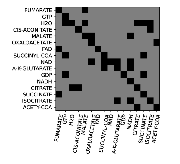
(a) Ground-truth

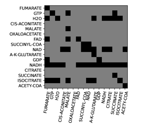
(b) DyNoTears on KrebsN

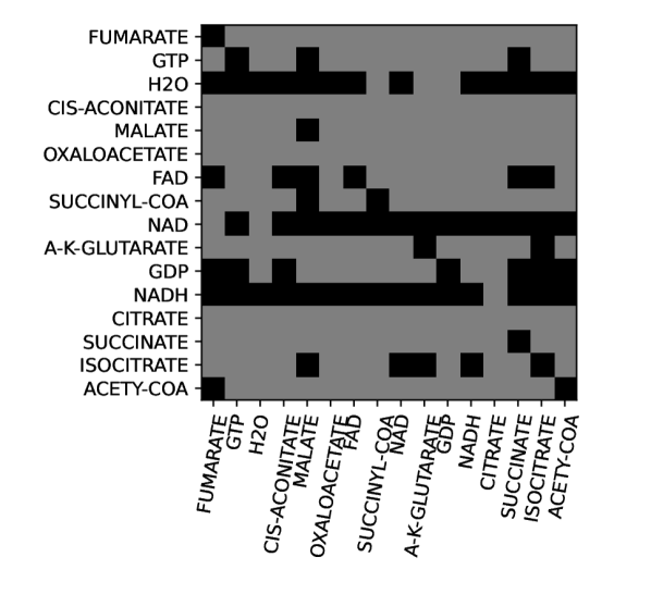
(c) DyNoTears on Krebs3

Figure 2: An illustration of the adjacency matrix produced by various methods, and the ground truth matrix representing the set of reactions.

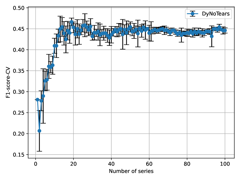
(a) KrebsN

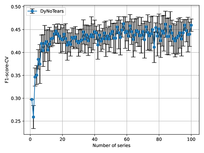
(b) Krebs3

Figure 3: An illustration of the F1-score of various methods on the Krebs dataset. Please note that the implementation of DyNoTears in CausalNex is deterministic, thus providing the same result each time. To calculate the error bars, randomly selected $10\,\%$ of the data were put aside, and then results were averaged over $10$ repeats of this procedure.

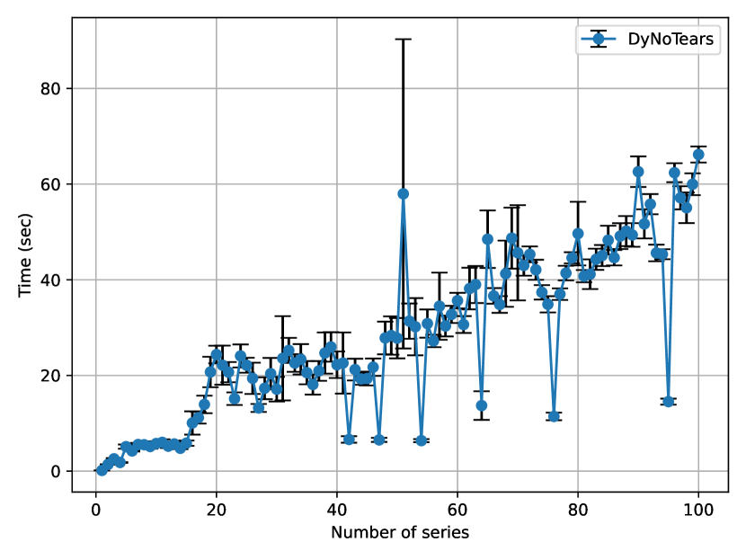
(a) KrebsN

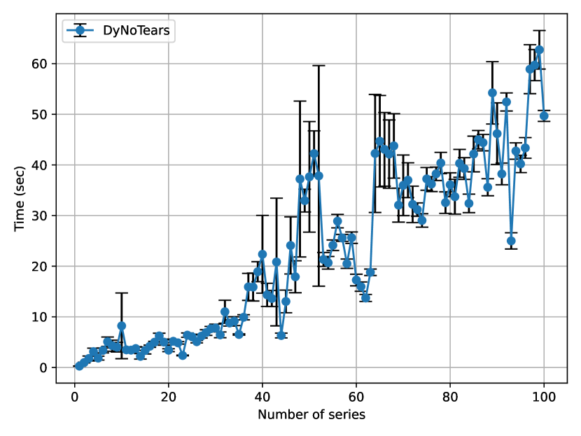
(b) Krebs3

Figure 4: An illustration of the time requriements of various methods on the Krebs dataset. The error bars show the standard deviation of the measurements calculated from $10$ repeats.

5 Conclusion

We publish all source files used to generate the data and the figures in this paper in the following GitHub repository https://github.com/petrrysavy/krebsdynotears. The repository also contains numeric results that were generated as input to the plots. The generator of the data can be found at https://github.com/petrrysavy/krebsgenerator, including a description of how to generate the benchmarking data. The generator is based on simulator at [18]. The dataset is available at https://huggingface.co/datasets/petrrysavy/krebs/tree/main.

References

- [1] Paul Beaumont, Ben Horsburgh, Philip Pilgerstorfer, Angel Droth, Richard Oentaryo, Steven Ler, Hiep Nguyen, Gabriel Azevedo Ferreira, Zain Patel, and Wesley Leong. CausalNex, October 2021.
- [2] Avrim Blum, Merrick Furst, Michael Kearns, and Richard J Lipton. Cryptographic primitives based on hard learning problems. In Annual International Cryptology Conference, pages 278–291. Springer, 1993.
- [3] Mehmet Caner and Bruce E Hansen. Instrumental variable estimation of a threshold model. Econometric theory, 20(5):813–843, 2004.
- [4] Yonghong Chen, Govindan Rangarajan, Jianfeng Feng, and Mingzhou Ding. Analyzing multiple nonlinear time series with extended granger causality. Physics Letters A, 324(1):26–35, 2004.
- [5] Y Choi, Antonio Vergari, and Guy Van den Broeck. Probabilistic circuits: A unifying framework for tractable probabilistic models. UCLA. URL: http://starai. cs. ucla. edu/papers/ProbCirc20. pdf, page 6, 2020.
- [6] Richard A Davis, Pengfei Zang, and Tian Zheng. Sparse vector autoregressive modeling. Journal of Computational and Graphical Statistics, 25(4):1077–1096, 2016.
- [7] Thomas Dean and Keiji Kanazawa. A model for reasoning about persistence and causation. Computational Intelligence, 5(2):142–150, 1989.
- [8] Peter Ebbes, Michel Wedel, Ulf Böckenholt, and Ton Steerneman. Solving and testing for regressor-error (in) dependence when no instrumental variables are available: With new evidence for the effect of education on income. Quantitative Marketing and Economics, 3:365–392, 2005.
- [9] C. W. J. Granger. Investigating causal relations by econometric models and cross-spectral methods. Econometrica, 37(3):424–438, 1969.
- [10] Reimar Hofmann and Volker Tresp. Discovering structure in continuous variables using bayesian networks. In Proceedings of the 8th International Conference on Neural Information Processing Systems, NIPS’95, page 500–506, Cambridge, MA, USA, 1995. MIT Press.
- [11] Maciej Kamiński, Mingzhou Ding, Wilson A. Truccolo, and Steven L. Bressler. Evaluating causal relations in neural systems: Granger causality, directed transfer function and statistical assessment of significance. Biological Cybernetics, 85(2):145–157, Aug 2001.
- [12] Armin Kekić, Bernhard Schölkopf, and Michel Besserve. Targeted reduction of causal models. arXiv preprint arXiv:2311.18639, 2023.
- [13] Jee-Seon Kim and Edward W. Frees. Multilevel modeling with correlated effects. Psychometrika, 72(4):505–533, Dec 2007.
- [14] Gaurav Mahajan, Sham Kakade, Akshay Krishnamurthy, and Cyril Zhang. Learning hidden markov models using conditional samples. In The Thirty Sixth Annual Conference on Learning Theory, pages 2014–2066. PMLR, 2023.
- [15] Mazen Melibari, Pascal Poupart, Prashant Doshi, and George Trimponias. Dynamic sum product networks for tractable inference on sequence data. In Conference on Probabilistic Graphical Models, pages 345–355. PMLR, 2016.
- [16] Ramaravind K. Mothilal, Amit Sharma, and Chenhao Tan. Explaining machine learning classifiers through diverse counterfactual explanations. In Proceedings of the 2020 Conference on Fairness, Accountability, and Transparency, FAT* ’20, page 607–617, New York, NY, USA, 2020. Association for Computing Machinery.
- [17] Kevin Patrick Murphy. Dynamic bayesian networks: representation, inference and learning. University of California, Berkeley, 2002.
- [18] August Nagro. Chemistry-engine. https://github.com/AugustNagro/Chemistry-Engine, 2015.
- [19] Leland Gerson Neuberg. Causality: Models, reasoning, and inference, by judea pearl, cambridge university press, 2000. Econometric Theory, 19(4):675–685, 2003.
- [20] Whitney K. Newey. Efficient instrumental variables estimation of nonlinear models. Econometrica, 58(4):809–837, 1990.
- [21] Mengjia Niu, Xiaoyu He, Petr Rysavy, Quan Zhou, and Jakub Marecek. Joint problems in learning multiple dynamical systems. arXiv preprint arXiv:2311.02181, 2023.
- [22] Roxana Pamfil, Nisara Sriwattanaworachai, Shaan Desai, Philip Pilgerstorfer, Konstantinos Georgatzis, Paul Beaumont, and Bryon Aragam. Dynotears: Structure learning from time-series data. In International Conference on Artificial Intelligence and Statistics, pages 1595–1605. Pmlr, 2020.
- [23] Judea Pearl. Bayesian netwcrks: A model cf self-activated memory for evidential reasoning. In Proceedings of the 7th conference of the Cognitive Science Society, University of California, Irvine, CA, USA, pages 15–17, 1985.
- [24] Judea Pearl. Chapter 2 - bayesian inference. In Judea Pearl, editor, Probabilistic Reasoning in Intelligent Systems, pages 29–75. Morgan Kaufmann, San Francisco (CA), 1988.
- [25] Jonas Peters, Dominik Janzing, and Bernhard Schölkopf. Elements of causal inference: foundations and learning algorithms. The MIT Press, 2017.
- [26] Hoifung Poon and Pedro Domingos. Sum-product networks: A new deep architecture. In 2011 IEEE International Conference on Computer Vision Workshops (ICCV Workshops), pages 689–690. IEEE, 2011.
- [27] Ali Shojaie and George Michailidis. Discovering graphical Granger causality using the truncating lasso penalty. Bioinformatics, 26(18):i517–i523, 09 2010.
- [28] Anastasios Tsiamis, Ingvar Ziemann, Nikolai Matni, and George J Pappas. Statistical learning theory for control: A finite-sample perspective. IEEE Control Systems Magazine, 43(6):67–97, 2023.
- [29] Arun Venkatraman, Wen Sun, Martial Hebert, J. Bagnell, and Byron Boots. Online instrumental variable regression with applications to online linear system identification. Proceedings of the AAAI Conference on Artificial Intelligence, 30(1), Mar. 2016.
- [30] Mike West and Jeff Harrison. Bayesian forecasting and dynamic models. Springer Science & Business Media, 2006.
- [31] Jan C Willems, Paolo Rapisarda, Ivan Markovsky, and Bart LM De Moor. A note on persistency of excitation. Systems & Control Letters, 54(4):325–329, 2005.
- [32] Axel Wismüller, Adora M. Dsouza, M. Ali Vosoughi, and Anas Abidin. Large-scale nonlinear granger causality for inferring directed dependence from short multivariate time-series data. Scientific Reports, 11(1):7817, Apr 2021.