\OneAndAHalfSpacedXI\TheoremsNumberedThrough\EquationsNumberedThrough
\RUNAUTHOR

Jacquillat and Li

\RUNTITLE

Learning to cover

\TITLE

Learning to cover: online learning and optimization with irreversible decisions

\ARTICLEAUTHORS\AUTHOR

Alexandre Jacquillat and Michael Lingzhi Li \AFF Sloan School of Management, Massachusetts Institute of Technology, Cambridge, MA 02142, \EMAILalexjacq@mit.edu
Technology and Operations Management, Harvard Business School, Cambridge, MA 02163, \EMAILmili@hbs.edu

\ABSTRACT

We define an online learning and optimization problem with irreversible decisions contributing toward a coverage target. At each period, a decision-maker selects facilities to open, receives information on the success of each one, and updates a machine learning model to guide future decisions. The goal is to minimize costs across a finite horizon under a chance constraint reflecting the coverage target. We derive an optimal algorithm and a tight lower bound in an asymptotic regime characterized by a large target number of facilities $m\to\infty$ but a finite horizon $T\in\mathbb{Z}_{+}$. We find that the regret grows sub-linearly at a rate $\Theta\left(m^{\frac{1}{2}\cdot\frac{1}{1-2^{-T}}}\right)$, thus converging exponentially fast to $\Theta(\sqrt{m})$. We establish the robustness of this result to the learning environment; we also extend it to a more complicated facility location setting in a bipartite facility-customer graph with a target on customer coverage. Throughout, constructive proofs identify a policy featuring limited exploration initially for learning purposes, and fast exploitation later on for optimization purposes once uncertainty gets mitigated. These findings underscore the benefits of limited online learning and optimization, in that even a few rounds can provide significant benefits as compared to a no-learning baseline.

\KEYWORDS

facility location, online learning, online optimization

1 Introduction

Organizations frequently face strategic planning decisions to develop networks capable of delivering efficient and reliable services. The facility location problem has grown into a central topic in operations research, with applications across supply chain management (Daskin 1997), power systems (Qi et al. 2015), telecommunications (Bardossy and Raghavan 2010), healthcare (Bertsimas et al. 2022, Jacquillat et al. 2024), public services (Aktaş et al. 2013), humanitarian operations (Bayram and Yaman 2018), etc. Across these domains, facilities are planned sequentially under uncertainty regarding the success or the performance of each facility. For instance, opening a telecommunications tower may be infeasible due to technical issues; a power plant may generate less power than expected due to environmental factors; a vaccination center may fail to achieve the immunization goal; and a retail store may bring lackluster profits due to lower-than-expected demand.

Increasingly, such uncertainty can be alleviated via predictive analytics and machine learning, using managerial, engineering, and environmental information for example. Whenever historical data is available, machine learning models can be built offline to inform strategic planning. However, predictive models may be unavailable for new technologies or processes, or may fail if the underlying systems change between data collection and deployment. Decision-makers can instead leverage online data from early deployments to build machine learning models and guide future planning decisions. This problem exhibits an online learning and optimization structure that needs to balance learning-based exploration (by delaying facility deployments until more information is available) and optimization-based exploitation (by opening facilities based on available information).

Let us outline three motivating examples falling into this general framework:

Example 1.1 (Clinical trials)

Due to the increasing complexity of late-stage randomized clinical trials, the average number of sites required to recruit sufficient subjects for meaningful treatment and control comparisons has grown to over 60 per trial (Brøgger-Mikkelsen et al. 2022). At the same time, 80% of clinical trials sites fail to meet their recruitment timeline (Johnson 2015), and up to 20% cease due to inadequate recruitment (Carlisle et al. 2015). Such risks create challenging problems to open clinical trials sites and recruit patient populations.

Example 1.2 (Retail stores)

Many retail stores close every year due to demographic, economic, and competitive factors. Thus, retailers need to learn the drivers of store performance and adaptively selecting locations for new stores to maximize coverage, sales and profitability.

Example 1.3 (Sustainable infrastructure)

Decarbonization pathways require rapid and large-scale infrastructure investments, including hundreds of GW of renewable generation, millions of electric vehicle chargers, and new industrial equipment (Pacala et al. 2021). Yet, around 5-10% of infrastructure projects are canceled or distressed, amounting to significant capital losses (Sakhrani 2015). This again requires adaptive decision-making to learn the environmental, technological and managerial characteristics of successful projects and inform future investments.

In practice, these processes are often conducted in an ad-hoc manner, with facility selection decisions reactively based on the performance of previous sites and on short-term targets. Instead, our main research question is how to select facilities to simultaneously contribute to overall coverage and generate data for future decisions. Specifically, we propose a theoretical framework for online learning and optimization with irreversible decisions toward target coverage:

  • Online learning and optimization. Facility selection generates data to train a machine learning model on facility success. This setting creates a “catch-22” situation, where a proficient machine learning algorithm requires a large sample, whereas optimal decisions require prior training of the machine learning model. This paper therefore embeds an online learning structure into a multi-stage stochastic optimization problem with endogenous uncertainty.

  • Target coverage. The goal is to achieve a desired coverage level by the end of a planning horizon, which can take the form of a target on successful facilities or on demand coverage. Due to underlying uncertainty, we formalize a probabilistic target via a chance constraint.

  • Irreversible decisions. Early facility deployments cannot be amended upon obtaining a better predictive model. This commitment creates inter-temporal dependencies in the physical state of the system. Dependencies are exacerbated by the finite horizon: in practice, on-the-ground studies can be time-consuming to assess facility success and decision-makers often need to achieve high coverage levels quickly. This environment only allows a few iterations in the online learning and optimization framework. These features restrict the applicability of asymptotically optimal explore-then-commit algorithms from the multi-armed bandit literature.

We address this problem via a finite-horizon sequential decision-making model with online learning. The decision-maker can open candidate facilities over $T$ periods. Each facility is associated with a vector of covariates. At each period, the decision-maker attempts to open facilities—an irreversible decision. By the next period, the decision-maker receives information on the success of each facility. This information can then be used to train a machine learning model that predicts the success of remaining facilities. The objective is to minimize the total cost of facility openings, subject to the chance constraint reflecting target coverage by the end of the horizon. We seek a policy that achieves minimal regret over a clairvoyant benchmark based on perfect information.

The model incorporates a general-purpose characterization of the machine learning model without relying on generative assumptions on the “true” relationship between covariates and outcomes, nor on parametric assumptions on the machine learning model. Instead, we leverage statistical theory results to express the generalization error rate as a function of the square root of the sample size—we also generalize our findings to broader learning functions. This characterization captures the exploration-exploitation trade-off by balancing the need to mitigate prediction error by acquiring more data versus avoiding misguided early decisions based on poorly-performing predictive models. This trade-off is reinforced by the irreversible decisions in our setting.

Main results and contributions.

Our main result is that the optimal regret grows at a rate of $\Theta\left(\varepsilon\cdot m^{\frac{1}{2}\cdot\frac{1}{1-2^{-T}}}\right)$, where $m$ denotes a coverage target (on facilities or customers) and $\varepsilon$ characterizes the uncertainty. This expression provides an asymptotically tight regret rate as the coverage target $m$ grows to infinity but the planning horizon $T$ remains finite. Through constructive proofs, we also provide simple and interpretable algorithms for facility deployments that achieve asymptotically optimal regret without requiring a priori knowledge of the machine learning model. The online learning and optimization approach therefore achieves sub-linear regret asymptotically.

We first derive our core result in a setting with a target on facilities, in which a decision-maker minimizes the cost of facility deployments while ensuring that $m$ facilities are successful with high probability by the end of the horizon. A perfect-information benchmark opens exactly $m$ facilities. We establish a lower bound on the regret from a deterministic approximation of the stochastic problem, using a leading-order analysis. We construct an algorithm that adds a buffer to the deterministic solution to handle uncertainty; we prove that its solution is asymptotically feasible and optimal as the number of targeted facilities grows to infinity ($m\to\infty$). Notably, the algorithm gives rise to a policy where the number of facility openings is concave in the target $m$. This structure suggests a limited-exploration strategy that tentatively opens a few facilities initially to enable learning while avoiding misguided decisions, and a fast exploitation strategy later on to meet the target by opening most facilities once uncertainty is mitigated via a stronger predictive model.

We establish the robustness of these findings to the learning environment. We first assume that the learning error decays in $\mathcal{O}(1/n^{r})$ rather than $\mathcal{O}(1/\sqrt{n})$ (where $n$ denotes the sample size). In that case, the optimal regret grows in $\Theta\left(\varepsilon\cdot m^{\frac{1-r}{1-r^{T}}}\right)$ when $r\neq 1$ and in $\Theta\left(\varepsilon\cdot m^{1/T}\right)$ when $n=1$. In particular, the algorithm achieves bounded regret in the case of linear learning (i.e., if the error rate is in $\mathcal{O}(1/n)$ or better) as the planning horizon grows infinitely. We then account for the possibility of acquiring data offline to warm start the machine learning model. This extension does not change the regret rate, thus suggesting a limited role of offline learning—even in a finite and limited planning horizon. These additional results underscore the robustness of the sub-linear asymptotic regret rate in our online learning and optimization model with irreversible decisions.

We then extend our main result to a more complex optimization environment characterized by a bipartite facility-customer coverage graph and a target on customers. In this setting, a decision-maker minimizes the cost of facility deployments while ensuring that $m$ customers get served with high probability. We find that, under stationarity and degree assumptions, the optimal regret still grows in $\Theta\left(\varepsilon\cdot m^{\frac{1}{2}\cdot\frac{1}{1-2^{-T}}}\right)$. Although the result is similar, the proof is complicated by two main factors. First, customer coverage does not merely depend on the number of facilities but on the set of successful facilities; in turn, we use the concentration inequality in dependency graphs from Janson (2004) to bound the difference between customer coverage under the stochastic solution and its deterministic approximation. Second, the perfect-information benchmark is no longer known due to combinatorial complexity surrounding facility location decisions; thus, we derive sensitivity analysis results to bound the difference between the perfect-information solution (which achieves a coverage of $m$ customers) and the stochastic solution (which adds a buffer due to uncertainty).

A difficulty in the graph setting is that the algorithm relies on a mixed-integer non-convex optimization formulation at each iteration. Thus, we conclude with a solution procedure to derive high-quality solutions and insights into the optimized learning and optimization strategy. Specifically, we find that the model at the core of the algorithm targets facilities by increasing order of expected incremental coverage. In other words, the algorithm ignores the least impactful facilities; it initially targets moderately impactful facilities for learning-based exploration; and it then opens the most impactful facilities once uncertainty is mitigated for optimization-based exploitation. We leverage that structure to design an optimal solution procedure in star graphs and a heuristic extension in general bipartite graphs. Computational results confirm and extend our theoretical findings in terms of learning-based exploration and optimization-based exploitation, sub-linear asymptotic regret, and diminishing returns of online learning as the planning horizon grows longer.

From a practical standpoint, the sub-linear regret rate underscores the benefits of limited online learning and optimization. This regret rate stands between the zero regret from a perfect-information benchmark and a linear regret from a single-stage no-learning baseline. Moreover, the optimal regret converges exponentially fast to the infinite-horizon limit of $\Theta\left(\varepsilon\cdot\sqrt{m}\right)$ as the planning horizon $T$ grows to infinity. These findings caution against both all-at-once optimization approaches to strategic planning under endogenous uncertainty, and prolonged rounds of online learning. Instead, limited online learning with just a few stages can be more practical to implement than more involved iterative procedures relying on a longer planning horizon; and it can also lead to near-optimal solutions that significantly outperform the no-learning baseline.

2 Literature Review

Facility location has grown into a canonical problem in operations research (Daskin 1997). Extensive literature focuses on facility location under demand uncertainty (see, e.g., Anthony et al. 2010, Baron et al. 2011, Taherkhani et al. 2020, Wang et al. 2023). Instead, our setting involves uncertainty on facility success. Daskin (1983) introduced the maximum expected covering location problem, where each facility has a given failure probability. The reliable facility location problem selects facilities under disruption risk, given that demand will need to be served by the surviving facilities (Snyder and Daskin 2005). This problem has been tackled via continuous approximations (Cui et al. 2010), two-stage stochastic programming (Laporte et al. 1994, Shen et al. 2011), robust optimization (Cheng et al. 2021), and distributionally robust optimization (Lu et al. 2015). Lim et al. (2013) showed that facility location decisions are sensitive to errors in the failure probabilities, motivating machine learning approaches to mitigate uncertainty.

Within the online optimization literature, irreversible decisions in our problem relate to Pandora’s problem (Brown and Uru 2024), online revenue management (Jasin and Kumar 2012, Bumpensanti and Wang 2020), the online multi-secretary problem (Arlotto and Gurvich 2019), and online resource allocation such as bin packing and generalized assignment (Vera and Banerjee 2021, Banerjee and Freund 2019, Baxi et al. 2024). In these problems, inter-temporal coupling stems from a shared budget under exogenous demand uncertainty. In contrast, our problem exhibits endogenous facility uncertainty and a chance constraint on coverage. In particular, facility opening decisions generate information on facility success, motivating online learning and optimization.

Our problem relates to the online facility location problem, which assigns each incoming customer to an existing facility or opens a new one (Fotakis 2011). Meyerson (2001) devised a randomized algorithm that achieves a constant approximation ratio under random order and a $\mathcal{O}(\log n)$ loss under adversarial arrivals. Fotakis (2008) improved the competitive ratio to $\mathcal{O}\left(\frac{\log n}{\log\log n}\right)$, which Cygan et al. (2018) extended to a case where customers arrive and leave dynamically. Kaplan et al. (2023) found a 3-competitive deterministic algorithm under random order. Guo et al. (2020) considered a networked setting in a facility-customer graph. Our problem considers facility uncertainty rather than demand uncertainty, and embeds online learning into online decision-making.

The diminishing returns in facility location also link to the dynamic submodular maximization problem, which seeks a subset of items to maximize a submodular function. Lattanzi et al. (2020b) and Monemizadeh (2020) derived $(1/2-\varepsilon)$-approximations; Agarwal and Balkanski (2023) proposed an algorithm that uses predictions on insertions and deletions. The related stochastic submodular cover problem seeks a subset that covers a submodular function under uncertainty regarding each item’s success. Goemans and Vondrák (2006) characterized the benefits of adaptivity; Agarwal et al. (2019) and Ghuge et al. (2022) showed that limited adaptivity can yield most of the benefits. Again, our paper differs by allowing online learning to mitigate uncertainty over time.

Recent extensions of the online facility location problem have incorporated predictions on facility-customer assignments to design algorithms that are $\mathcal{O}(1)$-competitive when predictions are good and $\mathcal{O}(\log n)$-competitive or $\mathcal{O}\left(\frac{\log n}{\log\log n}\right)$-competitive otherwise (Jiang et al. 2021, Fotakis et al. 2021). Almanza et al. (2021) obtained similar results with predictions on the set of facilities to open. This line of work falls into the broader literature on prediction-augmented online decision-making, with applications to packing, matching, scheduling, reource allocation, etc. (see, e.g., Lykouris and Vassilvitskii 2021, Lattanzi et al. 2020a, Lavastida et al. 2020, Jin and Ma 2022) Our problem embeds online learning into online decision-making as opposed to relying on offline advice.

Turning to the online learning and optimization literature, the multi-armed bandit problem uncovers the well-known trade-off between exploration and exploitation to learn each arm’s average reward and to select the best arm (Slivkins et al. 2019, Lattimore and Szepesvári 2020). In particular, contextual bandits leverage covariate information on each arm, by leveraging regularity assumptions to learn the relationship between contexts and rewards in Lipschitz and linear contextual bandits (Lu et al. 2010, Slivkins 2011, Chu et al. 2011), or by directly learning the optimal policy (Auer et al. 2002, Langford and Zhang 2007). In a facility location setting, Cao et al. (2021) optimized the location of mobile retail facilities; since each facility can be moved from one period to another, this problem was framed as a contextual bandit and solved using continuous approximations of spatial operations and the upper-confidence-bound algorithm.

Our paper departs from traditional bandit models in three ways. First, we derive results without relying on regularity assumptions and without restricting the class of admissible policies; instead, we use statistical learning theory to characterize the prediction error as a function of the sample size. Second, we seek results in an asymptotic regime with a large coverage target but a fixed horizon, which restricts the use of typical explore-then-commit algorithms. Third, we consider an online learning and optimization environment with irreversible decisions. Farias and Madan (2011) considered a bandit problem with irrevocable decisions in which an arm that was pulled earlier and then discarded cannot be pulled again. In our problem, all facilities that are successfully opened remain opened throughout the planning horizon and contribute to overall coverage. These dynamics create inter-temporal dependencies that augment the belief state in multi-armed bandits with a physical state to keep track of coverage, using the framework from Powell (2022). General-purpose algorithms to optimize the exploration-exploitation trade-off are much more challenging in these broader dynamic programming and reinforcement learning settings (Ryzhov et al. 2012, Russo and Van Roy 2018, Osband et al. 2019). In this paper, we formalize a class of online learning and optimization problems with target coverage and irreversible decisions, for which we derive asymptotically tight bounds and asymptotically optimal algorithms.

3 The Core Model: Target on Facilities

We define the core problem where the decision-maker aims to open a target number of facilities over a finite horizon, under uncertainty on facility success. In this setting, facilities are homogeneous, so we focus on the number of facilities to open—as opposed to the set of facilities. To isolate the core trade-off between learning and optimization, we assume that the machine learning model can only be trained using online data. We establish the robustness of our findings in different learning environments Section 3.4, and in more complex networked optimization environments in Section 4.

Throughout this paper, we adopt standard asymptotic notation: (i) $f(x)=\mathcal{O}(g(x))$ if there exist $M>0$ and $\bar{x}$ such that $f(x)\leq Mg(x)$ for all $x\geq\bar{x}$; (ii) $f(x)=o(g(x))$ if for all $M>0$ there exists $\bar{x}$ such that $f(x)\leq Mg(x)$ for all $x\geq\bar{x}$; (iii) $f(x)=\Omega(g(x))$ if there exist $M>0$ and $\bar{x}$ such that $f(x)\geq Mg(x)$ for all $x\geq\bar{x}$; and (iv) $f(x)=\Theta(g(x))$ if $f(x)=\mathcal{O}(g(x))$ and $f(x)=\Omega(g(x))$.

3.1 Problem statement

Optimization environment.

A decision-maker targets to open $m$ facilities over $T$ periods, stored in a set $\mathcal{T}=\{1,\cdots,T\}$. Let $\mathcal{F}$ denote the set of candidate facilities. Each facility involves uncertainty on its success, characterized via a binary indicator $v_{it}\in\{0,1\}$ for facility $i\in\mathcal{F}$ at time $t\in\mathcal{T}$. We assume that the $v_{it}$ realizations are revealed in the next period after the decision-maker attempts to open the facility and that they are independent across facilities. In our clinical trial example, the assumptions on the $v_{it}$ realizations corresponds to a setting where the recruitment potential can be determined by on-the-ground studies following site selection; and the independence assumption corresponds to a setting where recruits are non-overlapping across sites. In our retail and infrastructure examples, they reflect instances where the profitability of a store and the technical feasibility of a power plant are unknown a priori and depend on local factors.

We model the decision-making problem via two sets of decision variables: $A_{t}$ denotes the number of facilities that the decision-maker attempts to open at time $t\in\mathcal{T}$; and $B_{t}$ denotes the number of facilities that are successfully opened at time $t\in\mathcal{T}$, which depends on the number of attempts (captured by the variable $A_{t}$) and the success of these facilities (reflected in the $v_{it}$ realizations).

The decision-maker aims to minimize the number of facility that are tentatively opened, subject to a chance constraint ensuring that $m$ facilities will be opened by the end of the planning horizon with sufficiently high probability $1-\delta$. The problem, referred to as ($\mathcal{P}^{*}$), can be written as follows.

$\displaystyle\min\quad$ $\displaystyle\sum_{t=1}^{T}A_{t}$ ($\mathcal{P}^{*}$)
s.t. $\displaystyle\mathbb{P}\left[\sum_{t=1}^{T}B_{t}\geq m\right]\geq 1-\delta$
$\displaystyle B_{t}=\sum_{i=1}^{A_{t}}v_{it},\ \forall t\in\mathcal{T}$
At,Bt0,t𝒯formulae-sequencesubscript𝐴𝑡subscript𝐵𝑡0for-all𝑡𝒯\displaystyle A_{t},B_{t}\geq 0,\ \forall t\in\mathcal{T}

Throughout this paper, we do not make a priori distributional assumptions on the random variables $v_{it}$. Instead, we consider a machine learning environment where the decision-maker has access to predictions regarding the success of each facility at each time period based on online data.

Learning environment.

At each period, each facility is associated with a feature vector $\bm{x}_{it}\in\mathbb{R}^{p_{t}}$. We allow features to be time-varying, due to exogenous variations and information from earlier facility opening decisions. We assume that the learning population consists exactly of the set of facilities that have been tentatively opened, so the decision-maker has access to $N_{t-1}=\sum_{s=1}^{t-1}A_{s}$ labeled data points at each period $t$. We relax this assumption by incorporating offline data in Section 3.4. The decision-maker can then train a machine learning model to predict the binary indicators $v_{it}$ for the remaining $|\mathcal{F}|-N_{t-1}$ facilities, which we encore via a function $f_{t}(\bm{x}_{it})$.

The learning and optimization environment is summarized in Figure 1. At each period, the decision-maker determines the number of facility opening attempts via the decision variable $A_{t}$. Realizations of successful and unsuccessful facilities are then revealed, which elicit the variable $B_{t}$. Critically, successful facilities remain open until the end of the horizon and cannot be amended. Moreover, the observations of successful and unsuccessful facilities augment a labeled dataset to train a new machine learning model, which can then support decision-making at the next period. Note that predictions on facility success can vary over time, due to the time-varying features and, most importantly, to the data augmentation from online decisions. This environment highlights the three core features of our problem: online optimization (sequential facility openings over a multi-period horizon), online learning (updates to a machine learning model based on new information), and irreversible decisions (commitment to facilities at each time period).

$\cdots$ $t=1$ $t=2$ $t=3$Decisions$A_{1}$Realizations$\left(v_{i1}\right)_{i=1,\cdots,A_{1}}$, $B_{1}$Learning$\left(\bm{x}_{i2}\right)_{i\in\mathcal{F}}$, $f_{2}$Decisions$A_{2}$Realizations$\left(v_{i2}\right)_{i=1,\cdots,A_{2}}$, $B_{2}$Learning$\left(\bm{x}_{i3}\right)_{i\in\mathcal{F}}$, $f_{3}$Decisions$A_{3}$
Figure 1: Timeline of events. [White/black dots: facilities with positive/negative predictions; blue dots: facility opening attempts; green/red dots: successfully/unsuccessfully opened facilities.]

We leverage statistical learning theory to provide a general-purpose characterization of the learning function $f_{t}$. Specifically, Assumption 1 states that the prediction error decays in $\mathcal{O}(1/\sqrt{n})$ where $n$ is the sample size. This property is satisfied up to logarithmic factors by many machine learning algorithms, such as k-nearest-neighbors (Chaudhuri and Dasgupta 2014), logistic regression (Ng and Jordan 2001), decision trees (Mansour and McAllester 2000), naive Bayes (Ng and Jordan 2001), and random forest (Gao and Zhou 2020). This result has been obtained under several conditions and assumptions, including VC-dimension (Boucheron et al. 2005, Vapnik and Chervonenkis 2015), pseudo-dimension (Anthony et al. 1999, Pollard 2012), algorithmic stability (Bousquet and Elisseeff 2002, Feldman and Vondrak 2019), PAC-Bayes (McAllester 1998) and robustness (Xu and Mannor 2012). This property enables us to characterize the learning process via a non-parametric condition on the learning rate, without relying on generative assumptions on the statistical model nor on parametric assumptions on the machine learning model. In 6, we provide numerical evidence of decaying classification errors as a function of sample size, even in finite-sample settings, using five publicly available datasets from the University of California at Irvine (2020) (UCI). Additionally, we establish the robustness of our results to different learning functions in Section 3.4 to generalize our findings in broader online learning and optimization settings.

{assumption}

[Learning function] There exists $0<\varepsilon\leq 1$ such that the error of the machine learning model $f_{t}$ trained with $N_{t-1}$ samples is bounded by:

$\displaystyle\mathbb{P}_{t}(f_{t}(\bm{x}_{it})\neq v_{it})\leq\frac{\varepsilon}{\sqrt{N_{t-1}+1}},$

where the probability space comprises the $|\mathcal{F}|-N_{t-1}$ remaining facilities at the start of period $t\in\mathcal{T}$.

Throughout this paper, we assume conservatively that the learning error takes the upper bound given in Assumption 1. Then, the random variable $B_{t}$ follows a binomial distribution with $A_{t}$ trials and success probability $1-\frac{\varepsilon}{\sqrt{N_{t-1}+1}}$. Problem ($\mathcal{P}^{*}$) can then be re-written as follows:

$\displaystyle\min\quad$ $\displaystyle\sum_{t=1}^{T}A_{t}$ ($\mathcal{P}^{*}$)
s.t. $\displaystyle\mathbb{P}\left[\sum_{t=1}^{T}B_{t}\geq m\right]\geq 1-\delta$
$\displaystyle B_{t}\sim\operatorname{Bino}\left(A_{t},1-\frac{\varepsilon}{\sqrt{\sum_{s=1}^{t-1}A_{s}+1}}\right),\ \forall t\in\mathcal{T}$
At,Bt0,t𝒯formulae-sequencesubscript𝐴𝑡subscript𝐵𝑡0for-all𝑡𝒯\displaystyle A_{t},B_{t}\geq 0,\ \forall t\in\mathcal{T}

Benchmarks.

We define two benchmarks that will serve as references throughout the analysis:

  • A perfect-information benchmark: A clairvoyant decision-maker that knows all $v_{it}$ in advance will select exactly $m$ facilities whenever $v_{it}=1$. We measure the regret of our algorithm as the difference between the solution to Problem ($\mathcal{P}^{*}$) and this clairvoyant benchmark.

  • A no-learning baseline: Without predicting facility success, the problem reduces to single-stage chance-constrained optimization. This benchmark involves linear regret as the target $m$ grows large. Indeed, tentatively opening $A_{1}=\frac{m}{1-\varepsilon}$ facilities results in at least $m$ successful facilities with a probability around 0.5. Thus, for $\delta<0.5$, the decision-maker needs to open at least $\frac{m}{1-\varepsilon}$ facilities, hence at least $m+\varepsilon m$ facilities. We compare the optimal regret to this single-stage benchmark in order to quantify the benefits of online learning in Problem ($\mathcal{P}^{*}$).

3.2 An asymptotically optimal algorithm with sub-linear regret

Problem ($\mathcal{P}^{*}$) as currently formulated remains intractable due to facility uncertainty and the learning process. With the chance constraints, the problem is equivalent to a value-at-risk formulation (Uryasev et al. 2010), which is notoriously challenging. A typical approach in the optimization literature is to adopt a tractable approximation via the conditional value-at-risk (see Uryasev and Rockafellar (2001) for the seminal method and Chan et al. (2018), Chenreddy and Delage (2024), Wang et al. (2024) for recent applications). We instead propose a simple and interpretable algorithm to tackle the stochastic chance-constrained optimization formulation. We prove the asymptotic optimality of its solution as the target number of facilities grows infinitely, by showing its feasibility and deriving an asymptotically-tight lower bound with the same regret rate.

Throughout this analysis, we consider the asymptotic regime where $m\to\infty$ but where $T\geq 2$ is finite. This regime is motivated by our practical examples where a decision-maker needs to open a large number of facilities (e.g., clinical trials sites, retail stores, power plants). In these examples, each iteration can be time-consuming and expensive to conduct on-the-ground studies, whereas the decision-maker may need to achieve the coverage target relatively quickly—so that high-quality solutions may need to be obtained within a limited number of iterations.

For notational convenience, we introduce the following parameter $\alpha_{T}$. Immediate properties are that $1/2<\alpha_{T}<1$ as $T\geq 2$ and that $\alpha_{T}$ converges exponentially fast to $1$ as $T\to\infty$.

$$\alpha_{T}=\frac{1}{1-\frac{1}{2^{T}}}$$

Algorithm 1 describes our procedure to generate a solution for Problem ($\mathcal{P}^{*}$). This procedure involves tentatively opening $A^{\dagger}_{t}$ facilities in each period $t\in\mathcal{T}$, given as follows::

$$A^{\dagger}_{t}=4^{t-T\cdot\alpha_{T}\cdot\left(1-\frac{1}{2^{t}}\right)}\ell^{\alpha_{T}\cdot\left(1-\frac{1}{2^{t}}\right)},$$ (1)

where $\ell$ is the unique positive solution to the following equation:

$$\sum_{t=1}^{T}4^{t-T\cdot\alpha_{T}\cdot\left(1-\frac{1}{2^{t}}\right)}\ell^{\alpha_{T}\cdot\left(1-\frac{1}{2^{t}}\right)}=m+\varepsilon\cdot\frac{4(2^{T}-1)}{2^{T\cdot\alpha_{T}}}m^{\frac{1}{2}\cdot\alpha_{T}}+\sqrt{-\frac{1}{2}\log\frac{\delta}{2}}\sqrt{m}.$$ (2)
Algorithm 1 Algorithm to solve Problem ($\mathcal{P}^{*}$).
Initialization: $N^{\dagger}_{0}=0$.
Repeat, for $t=1,\cdots,T$:
  • 1. Optimize. Tentatively open $A^{\dagger}_{t}=4^{t-T\frac{1-2^{-t}}{1-2^{-T}}}\ell^{\frac{2^{T}(1-2^{-t})}{2^{T}-1}}$ facilities, where $\ell$ is given in Equation (2).

  • 2. Commit. Observe realizations $B^{\dagger}_{t}\sim\operatorname{Bino}\left(A^{\dagger}_{t},1-\frac{\varepsilon}{\sqrt{\sum_{s=1}^{t-1}A^{\dagger}_{s}+1}}\right)$, and update $N^{\dagger}_{t}=N^{\dagger}_{t-1}+B^{\dagger}_{t}$.

Theorem 3.1 provides the main result of this section, showing the asymptotically-tight sub-linear regret bound in $\Theta\left(m^{\frac{1}{2}\cdot\alpha_{T}}\right)$ from Problem ($\mathcal{P}^{*}$), the asymptotic feasibility of the solution from Algorithm 1, and its asymptotic optimality up to the second leading order.

Theorem 3.1

The optimal solution $m^{*}(\varepsilon,T)$ of Problem ($\mathcal{P}^{*}$) satisfies, as $m\to\infty$:

$$m^{*}(\varepsilon,T)=m+\varepsilon\cdot\frac{4(2^{T}-1)}{2^{T\cdot\alpha_{T}}}m^{\frac{1}{2}\cdot\alpha_{T}}+o\left(m^{\frac{1}{2}\cdot\alpha_{T}}\right),$$

if $\delta=o\left(m^{\frac{1}{2}\cdot\alpha_{T}-1}\right)$. Moreover, Algorithm 1 yields an asymptotically feasible solution to Problem ($\mathcal{P}^{*}$) with an objective value $m^{\dagger}(\varepsilon,T)$ that satisfies, as $m\to\infty$:

$$m^{\dagger}(\varepsilon,T)=m+\varepsilon\cdot\frac{4(2^{T}-1)}{2^{T\cdot\alpha_{T}}}m^{\frac{1}{2}\cdot\alpha_{T}}+o\left(m^{\frac{1}{2}\cdot\alpha_{T}}\right).$$

The proofs of this theorem and all auxiliary results are provided in 7. We provide an overview of the proof below, including three main lemmas that provide technical insights into the problem.

Proof 3.2

Sketch of the proof.

We define a deterministic approximation of the problem for $\delta=0$, where $B_{t}$ always realizes at the mean value. The problem, referred to as Problem ($\mathcal{P}^{D}$), is given by:

$\displaystyle\min\ \left\{\ \sum_{t=1}^{T}A_{t}\ \ \bigg{|}\ \ \sum_{t=1}^{T}A_{t}\left(1-\frac{\varepsilon}{\sqrt{\sum_{s=1}^{t-1}A_{s}+1}}\ \right)\geq m\right\}.$ ($\mathcal{P}^{D}$)

We elicit the asymptotic solution of Problem ($\mathcal{P}^{D}$) in Lemma 3.3. The proof of this result relies on expressing the Karush–Kuhn–Tucker (KKT) conditions and performing leading-order and leading-coefficient analyses to identify the asymptotic dependency on $m$ in the non-linear equation.

Lemma 3.3 (Asymptotic solution of Problem ($\mathcal{P}^{D}$))

Let $m^{D}(\varepsilon,T)$ be the optimal objective value of Problem ($\mathcal{P}^{D}$), and $A^{D},\cdots,A^{D}$ be its solution. For any $T\geq 2$, we have as $m\to\infty$:

$\displaystyle A^{D}_{t}=4^{t-T\cdot\alpha_{T}\cdot\left(1-\frac{1}{2^{t}}\right)}m^{\alpha_{T}\cdot\left(1-\frac{1}{2^{t}}\right)}+o\left(m^{\alpha_{T}\cdot\left(1-\frac{1}{2^{t}}\right)}\right),\ \forall t=1,\cdots,T,$ (3)
$\displaystyle m^{D}(\varepsilon,T)=m+\varepsilon\cdot\frac{4(2^{T}-1)}{2^{T\cdot\alpha_{T}}}m^{\frac{1}{2}\cdot\alpha_{T}}+o\left(m^{\frac{1}{2}\cdot\alpha_{T}}\right).$ (4)

This result serves as a technical lemma to prove the main theorem. Moreover, the solution of the deterministic problem provides insights into the structure of the optimal solution of the stochastic problem. In fact, the intuition behind Equation (2) and Algorithm 1 is to construct a solution that is similar to the one from Equation (3), plus a buffer to handle facility uncertainty. This observation follows from the fact that $\ell$ is on the order of $\Theta(m)$, which we prove in Remark 3.4.

Remark 3.4

Let $\ell$ be the unique positive solution to Equation (2). We have:

$$\frac{3m}{4}\leq\ell\leq m+\varepsilon\cdot\frac{4(2^{T}-1)}{2^{T\cdot\alpha_{T}}}m^{\frac{1}{2}\cdot\alpha_{T}}+\sqrt{-\frac{1}{2}\log\frac{\delta}{2}}\sqrt{m}.$$

We can then show that the solution given by Algorithm 1 satisfies the chance constraint as $m\to\infty$, and therefore provides an asympotically feasible solution of the stochastic problem ($\mathcal{P}^{*}$). Thus, the solution of Algorithm 1 provides an upper bound to Problem ($\mathcal{P}^{*}$). The proof of the lemma leverages Hoeffding’s inequality across time periods $1,\cdots,T$, by expressing each value of $\mathbb{E}(B_{t})$ from Equations (1)–(2). This bounds the probability that at least $m$ facilities get successfully opened by the end of the planning horizon.

Lemma 3.5 (Upper bound)

The policy given in Equation (1) and Algorithm 1 satisfies:

$$\lim_{m\to\infty}\mathbb{P}(N^{\dagger}_{T}\geq m)\geq 1-\delta.$$

Finally, we establish the lower bound of Theorem 3.1 in Lemma 3.6. The proof of this result first shows that the number of successful facilities $B_{t}$ remains close to its expected value at each time $t=1,\cdots,T$, by using Hoeffding’s inequality across facilities at each time period and the union bound across time periods. It then calls Lemma 3.3 conditionally on the event that $B_{1}\approx\mathbb{E}(B_{1}),\cdots,B_{T}\approx\mathbb{E}(B_{T})$ to bound the total number of facilities $m^{*}(\varepsilon,T)$ that need to be tentatively opened.

Lemma 3.6 (Lower bound)

Assume that $\delta=o\left(m^{\frac{1}{2}\cdot\alpha_{T}-1}\right)$. Let $m^{*}(\varepsilon,T)$ denote the optimal solution of Problem ($\mathcal{P}^{*}$). The following holds, as $m\to\infty$:

$$m^{*}(\varepsilon,T)\geq m+\varepsilon\cdot\frac{4(2^{T}-1)}{2^{T\cdot\alpha_{T}}}m^{\frac{1}{2}\cdot\alpha_{T}}+o\left(m^{\frac{1}{2}\cdot\alpha_{T}}\right)$$

Together, the lemmas show that the strategy detailed in Algorithm 1 is asymptotically optimal up to second-leading order terms, therefore completing the proof of the theorem. \Halmos

3.3 Discussion of results and managerial implications

We conclude with a theoretical and practical interpretation of the results provided in Theorem 3.1. To guide the discussion, we illustrate the regret expressions and the policy in Table 1 for different coverage targets (i.e., different values of $m$) and planning horizons (i.e., different values of $T$).

Table 1: Theoretical and numerical expressions of the regret and facility opening policy ($\varepsilon=0.4$, $\delta=1\%$).
Expression Metric $T=2$ $T=3$ $T=4$ $T=5$ $T=6$
Theory No-learning regret $\Theta(\varepsilon m)$ $\Theta(\varepsilon m)$ $\Theta(\varepsilon m)$ $\Theta(\varepsilon m)$ $\Theta(\varepsilon m)$
$(m\to\infty)$ Online regret $\Theta(1.9\varepsilon m^{0.67})$ $\Theta(2.6\varepsilon m^{0.57})$ $\Theta(3.1\varepsilon m^{0.53})$ $\Theta(3.5\varepsilon m^{0.52})$ $\Theta(3.7\varepsilon m^{0.51})$
Policy $A^{\dagger}_{t}$ ($t=1$) $\Theta(0.63m^{0.67})$ $\Theta(0.37m^{0.57})$ $\Theta(0.21m^{0.53})$ $\Theta(0.11m^{0.52})$ $\Theta(0.06m^{0.51})$
Policy $A^{\dagger}_{t}$ ($t=2$) $\Theta(m)$ $\Theta(0.45m^{0.86})$ $\Theta(0.19m^{0.80})$ $\Theta(0.07m^{0.77})$ $\Theta(0.03m^{0.76})$
Policy $A^{\dagger}_{t}$ ($t=3$) $\Theta(m)$ $\Theta(0.36m^{0.93})$ $\Theta(0.12m^{0.90})$ $\Theta(0.04m^{0.89})$
Policy $A^{\dagger}_{t}$ ($t=4$) $\Theta(m)$ $\Theta(0.31m^{0.97})$ $\Theta(0.09m^{0.95})$
Policy $A^{\dagger}_{t}$ ($t=5$) $\Theta(m)$ $\Theta(0.29m^{0.98})$
Policy $A^{\dagger}_{t}$ ($t=6$) $\Theta(m)$
Numerical No-learning regret 93 93 93 93 93
$(m=100)$ Online regret 34 32 33 34 34
Policy $A^{\dagger}_{t}$ ($t=1$) 16 6 3 2 $<1$
Policy $A^{\dagger}_{t}$ ($t=2$) 118 24 8 3 1
Policy $A^{\dagger}_{t}$ ($t=3$) 102 26 8 3
Policy $A^{\dagger}_{t}$ ($t=4$) 96 26 8
Policy $A^{\dagger}_{t}$ ($t=5$) 95 26
Policy $A^{\dagger}_{t}$ ($t=6$) 96
Numerical No-learning regret 746 746 746 746 746
$(m=1,000)$ Online regret 128 108 103 103 105
Policy $A^{\dagger}_{t}$ ($t=1$) 66 19 8 4 2
Policy $A^{\dagger}_{t}$ ($t=2$) 1,062 159 42 14 5
Policy $A^{\dagger}_{t}$ ($t=3$) 930 198 53 16
Policy $A^{\dagger}_{t}$ ($t=4$) 855 208 56
Policy $A^{\dagger}_{t}$ ($t=5$) 824 210
Policy $A^{\dagger}_{t}$ ($t=6$) 816
  • No-learning regret: regret of the no-learning single-stage baseline; online regret: regret of Algorithm 1.

Asymptotically-tight bounds.

Theorem 3.1 provides upper-bounding and lower-bounding approximations of the optimal solution of Problem ($\mathcal{P}^{*}$), therefore deriving asymptotically-tight rates up to second-leading order terms. Recall that the perfect-information benchmark opens exactly $m$ facilities. Thus, the result yields an asymptotically-tight regret expression as follows:

$$\texttt{Regret}=\varepsilon\cdot\frac{4(2^{T}-1)}{2^{T\cdot\frac{1}{1-\frac{1}{2^{T}}}}}m^{\frac{1}{2}\cdot\frac{1}{1-\frac{1}{2^{T}}}}+o\left(m^{\frac{1}{2}\cdot\frac{1}{1-\frac{1}{2^{T}}}}\right).$$

The asymptotic feasibility guarantee and upper bound are always valid; in contrast, the lower bound is valid for a sufficiently strong chance constraint, captured by the condition $\delta=o\left(m^{\frac{1}{2}\cdot\alpha_{T}-1}\right)$. This restriction is rather weak, ranging from $\delta=o\left(\frac{1}{m^{1/3}}\right)$ with $T=2$ to $\delta=o\left(\frac{1}{\sqrt{m}}\right)$ as $T\to\infty$. These conditions translate into feasibility guarantees of at least 80–90% with $m=100$ and 90–97% with $m=1,000$ facilities, which are usually consistent with desired reliability targets in practice.

Sub-linear regret: benefits of online learning.

Recall that the no-learning baseline induces a linear regret by opening at least $m+\varepsilon m$ facilities. By achieving sub-linear asymptotic regret, the learning-enhanced approach therefore achieves an intermediate outcome between the perfect-information benchmark and the no-learning baseline. Specifically, the learning-enhanced approach results in $m+\Theta\left(\varepsilon\cdot m^{2/3}\right)$ tentative facility openings with $T=2$ down to $m+\Theta\left(\varepsilon\cdot\sqrt{m}\right)$ tentative facility openings as $T\to\infty$. As expected, the algorithm’s loss increases proportionally with the error term $\varepsilon$, which reflects the extent of uncertainty. Most importantly, the sub-linear rate of regret highlights the strong performance improvements of the online learning and optimization approach upon the no-learning baseline. Numerically, these benefits translate into significant cost savings, estimated at 30–40% (e.g., 193 vs. 134 with $m=100$, 1,746 vs. 1,128 with $m=1,000$ in Table 1).

Exponential rate of convergence: fast learning.

Recall that the sub-linear regret holds in an asymptotic regime with an infinite number of facilities and any finite horizon. Still, the dependency on $T$ indicates that the sub-linear regret rate decreases exponentially fast as the planning horizon grows longer—reflected in the $\frac{1}{1-2^{-T}}$ factor in the regret rate. Specifically, the regret rate converges to $\Theta(\varepsilon\sqrt{m})$ as $T\to\infty$ and, in limited planning horizons, the regret rate grows in $\Theta(\varepsilon\cdot m^{0.67})$ with $T=2$, in $\Theta(\varepsilon\cdot m^{0.57})$ with $T=3$, in $\Theta(\varepsilon\cdot m^{0.53})$ with $T=4$ (Table 1). We therefore obtain a regret rate close to the long-term rate of $\Theta(\varepsilon\sqrt{m})$ with as few as 3-5 iterations.

This observation underscores the benefits of limited online learning. Indeed, even a few stages of learning can yield significant gains, by inducing a sub-linear regret rate of $\Theta(\varepsilon\cdot m^{0.53})$ to $\Theta(\varepsilon\cdot m^{0.67})$ with 2–4 iterations of online learning, as opposed to a linear regret rate of $\Theta(\varepsilon\cdot m)$ under the no-learning single-stage baseline. Conversely, more iterations bring more marginal benefits, by bringing the regret rate down from $\Theta(\varepsilon\cdot m^{0.53})$ with 4 iterations to $\Theta(\varepsilon\sqrt{m})$ in an infinite horizon.

An asymptotically optimal algorithm.

The proof of Theorem 3.1 is constructive, and yields a simple and interpretable algorithm that attempts to open $4^{t-T\cdot\alpha_{T}\cdot\left(1-\frac{1}{2^{t}}\right)}\ell^{\alpha_{T}\cdot\left(1-\frac{1}{2^{t}}\right)}$ facilities in each period $t=1,\cdots,T$, where $\ell=\Theta(m)$ (Remark 3.4). This policy is monotonically increasing but concave with the target number of facilities. This suggests that a few facilities get tentatively opened in initial iterations and that, conversely, the bulk of facilities get opened later on once uncertainty gets partially mitigated. For example, when $T=2$, the decision-maker attempts to opens $\Theta(m^{2/3})$ facilities in the first period and $\Theta(m)$ facilities in the second period; when $T=3$, the sequence is $\Theta(m^{0.57})$, $\Theta(m^{0.86})$, and $\Theta(m)$ facilities. Moreover, as $T$ grows to $\infty$, the first-period decision is $\Theta\left(\frac{\sqrt{m}}{2^{T-2}}\right)$, so that it is sufficient to consider a horizon of $\frac{1}{2}\log_{2}(m)$ (otherwise, the first-period decision involves not even building one facility). In other words, a logarithmic horizon is sufficient to achieve the full benefits of an infinite-horizon online learning algorithm. This observation further highlights the exponentially fast convergence, hence the benefits of limited online learning.

Practical implications.

These findings caution against both all-at-once approaches to strategic planning under uncertainty and prolonged rounds of online learning. Instead, they recommend a phased approach that integrates joint learning and optimization in an online decision-making environment. The concave policy highlights the exploration-exploitation trade-off in the context of irreversible decisions. Early iterations involve limited exploration to gather information on successful and unsuccessful facilities, driven by the need to avoid costly early commitments. In later iterations, the strategy shifts to fast exploitation, using the latest machine learning models to open the majority of facilities and meet the coverage target. The rapid convergence in regret rates suggests that near-optimal costs can be achieved in just a few iterations over a limited planning horizon, thereby realizing the benefits of online learning and optimization even when information gathering is time-consuming to acquire and when coverage targets must be met rapidly.

3.4 Robustness to the learning environment

Learning function.

Recall that Assumption 1 characterizes a prediction error that decays to zero at a rate of $\mathcal{O}(1/\sqrt{n})$. We relax this assumption to show the robustness of our findings on the benefits of online learning and optimization to the learning function.

First, the learning rate can differ from $\mathcal{O}(1/\sqrt{n})$. Several non-parametric methods, such as decision trees and Bayesian additive regression trees, can exhibit slower convergence (Ročková and Saha 2019, Mazumder and Wang 2024). On the other hand, under some assumptions, certain machine learning models can achieve faster convergence, up to $\mathcal{O}(1/n)$ (Sridharan et al. 2008, Jin et al. 2018). Accordingly, we consider a more general error rate $\mathcal{O}(1/n^{r})$, where $r>0$. The new problem $(\mathcal{P}^{*}_{r})$ is identical to Problem ($\mathcal{P}^{*}$) except that the variables $B_{t}$ are given by:

$$B_{t}\sim\operatorname{Bino}\left(A_{t},1-\frac{\varepsilon}{\left(\sum_{s=1}^{t-1}A_{s}+1\right)^{r}}\right),\ \forall t\in\mathcal{T}.$$ (5)

We adjust Algorithm 1 to account for the learning rate (Equation (17) in 7.6). Notably, the number of facilities tentatively opened at period $t$ grows in $\Theta\left(m^{\frac{1-r^{t}}{1-r^{T}}}\right)$ when $r\neq 1$; in particular, the faster the learning rate, the fewer facilities get tentatively opened initially to take advantage of the learning opportunities. Theorem 3.7 states that the regret rate grows in $\Theta\left(m^{\frac{1-r}{1-r^{T}}}\right)$ when $r\neq 1$, and in $\Theta(m^{1/T})$ when $r=1$. The asymptotic regret rate is visualized in Figure 2.

Theorem 3.7

Define $f_{r}(T)=\frac{1-r}{1-r^{T}}$ for $r\neq 1$ and $f_{1}(T)=1/T$. Assume that $\delta(m^{f(T)-1})$. The optimal solution of Problem $(\mathcal{P}^{*}_{r})$ and the algorithm’s solution satisfy, as $m\to\infty$:

$$m^{*}(\varepsilon,T)=m+\Theta\left(\varepsilon\cdot m^{f_{r}(T)}\right)\ \text{and}\ m^{\dagger}(\varepsilon,T)=m+\Theta\left(\varepsilon\cdot m^{f_{r}(T)}\right)$$

.

Refer to caption
(a)
Refer to caption
(b)
Figure 2: Impact of learning rate and time horizon on asymptotic regret rate (Theorem 3.7).

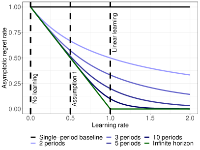
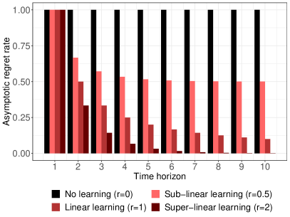
As expected, the regret decreases as the learning rate increases. As $T$ goes to infinity (green line in Figure 2(a)), the asymptotic regret rate converges to $1-r$ when $r<1$ and to 0 when $r\geq 1$. In particular, the algorithm achieves a regret of $\Theta(m^{1-r})$ when $r<1$ as the horizon grows larger. Interestingly, this result also implies that the algorithm achieves a bounded regret in the double-asymptotic regime where $m$ and $T$ grow to infinity at comparable rates (e.g., $m=\rho^{a}$ and $T=\rho^{b}$ with $a,b>1$ and $\rho\to\infty$). Note, also, that the convergence of the regret rate undergoes a phase transition in $r=1$, moving from exponential convergence when $r\neq 1$ to linear convergence when $r=1$ back to exponential convergence when $r>1$ (Figure 2(b)). Altogether, these results extend our main findings regarding the sub-linear regret rate and the asymptotic optimality of the algorithm, which demonstrates the robustness of the benefits of online learning across a wide range of regimes.

In our second extension, we incorporate an irreducible error term $1-p$ to capture instances where the predictive model cannot reach perfect prediction accuracy as the sample size increases. By design, the problem interpolates between the no-learning benchmark (with $p=0$) and the setting from Section 3 (with $p=1$). The new problem $(\mathcal{P}^{*}_{Imp})$ features the following dynamics:

$$B_{t}\sim\operatorname{Bino}\left(A_{t},1-\frac{\varepsilon p}{\sqrt{\sum_{s=1}^{t-1}A_{s}+1}}-\varepsilon(1-p)\right),\ \forall t\in\mathcal{T}.$$ (6)

Again, we adjust Algorithm 1 to account for the residual error term (Equation (18) in 7.7). We compare its solution to an offline benchmark armed with the best possible machine learning model; this benchmark retains an $\varepsilon(1-p)$ error, and therefore needs to open at least $\frac{1}{1-\varepsilon(1-p)}m$ facilities. Theorem 3.8 shows that our algorithm yields an asymptotically optimal solution and that Problem $(\mathcal{P}^{*}_{Imp})$ still achieves sub-linear regret against the offline benchmark.

Theorem 3.8

Assume that $\delta=o\left(m^{\frac{1}{2}\cdot\alpha_{T}-1}\right)$, the optimal solution of Problem $(\mathcal{P}^{*}_{Imp})$ and the algorithm’s solution, denoted by $m^{*}(\varepsilon,T)$ and $m^{\dagger}(\varepsilon,T)$ respectively, satisfy, as $m\to\infty$:

$\displaystyle m^{*}(\varepsilon,T)$ $\displaystyle=\frac{1}{1-\varepsilon(1-p)}m+\frac{\varepsilon p}{1-\varepsilon(1-p)}\cdot\frac{4(2^{T}-1)}{2^{T\cdot\alpha_{T}}}\cdot m^{\frac{1}{2}\cdot\alpha_{T}}+o\left(m^{\frac{1}{2}\cdot\alpha_{T}}\right),$
$\displaystyle m^{\dagger}(\varepsilon,T)$ $\displaystyle=\frac{1}{1-\varepsilon(1-p)}m+\frac{\varepsilon p}{1-\varepsilon(1-p)}\cdot\frac{4(2^{T}-1)}{2^{T\cdot\alpha_{T}}}\cdot m^{\frac{1}{2}\cdot\alpha_{T}}+o\left(m^{\frac{1}{2}\cdot\alpha_{T}}\right).$

Offline data.

We now relax the assumption that data are only available online. In practice, the decision-maker may warm start the predictive model prior to committing to online facility openings. We therefore augment the model with a zero-th time period, with decision variable $A_{0}$ reflecting the number of data points acquired offline at a cost $0<c\leq 1$. The offline sample impacts the error of the machine learning model but does not contribute toward meeting the target of $m$ facilities. A cost $c=1$ mirrors the setting in Section 3; with $c<1$, offline data acquisition offers cheaper learning opportunities without committing to facility openings.

The new problem, referred to as $(\mathcal{P}^{*}_{WS})$, features two differences with Problem ($\mathcal{P}^{*}$): (i) it minimizes the total cost $cA_{0}+\sum_{t=1}^{T}A_{t}$; and (ii) the number of successful facilities at time $t$ satisfies:

$$B_{t}\sim\operatorname{Bino}\left(A_{t},1-\frac{\varepsilon}{\sqrt{A_{0}+\sum_{s=1}^{t-1}A_{s}+1}}\right),\ \forall t\in\mathcal{T}$$

We adjust the algorithm to account for the warm-start opportunities as follows:

$\displaystyle A^{\dagger}_{0}$ $\displaystyle=\left(\frac{2\varepsilon}{c}\cdot\frac{\alpha_{T}(2^{T}-1)}{2^{T\cdot\alpha_{T}}}\right)^{\frac{2}{\alpha_{T}+2}}\cdot\ell^{\frac{1}{2}\cdot\alpha_{T+1}}$ (7)
$\displaystyle A^{\dagger}_{t}$ $\displaystyle=4^{t-T\cdot\alpha_{T}\cdot\left(1-\frac{1}{2^{t}}\right)}\cdot\left(\frac{2\varepsilon}{c}\cdot\frac{\alpha_{T}(2^{T}-1)}{2^{T\cdot\alpha_{T}}}\right)^{\frac{-2\alpha_{T}}{\alpha_{T}+2}\left(1-\frac{1}{2^{t}}\right)}\cdot\ell^{\alpha_{T+1}\left(1-\frac{1}{2^{t+1}}\right)},\ \forall t=1,\cdots,T,$ (8)

where $\ell$ is the solution to an implicit equation akin to Equation (2) (Equation (19) in 7.8). Note that the decision-maker takes advantage of the warm-starting opportunities to alleviate the cost of prediction errors in the online algorithm: as the cost $c$ decreases and as the statistical error $\varepsilon$ increases, more data are acquired offline and comparatively fewer facilities need to be opened during the actual planning horizon. Still, the number of offline data samples grows in $\Theta\left(m^{\frac{1}{2}\cdot\alpha_{T+1}}\right)$, which matches the rate of the first-period decision in the core setting with a planning horizon of $T+1$ (Equation (1)). In other words, offline learning merely “shifts” the first-period decision ($t=1$ with a planning horizon of $T+1$ periods) to the zero-th period ($t=0$ with a planning horizon of $T$ periods), irrespective of the cost $c$ of offline data.

In fact, Theorem 3.9 shows that the new regret rate is identical to the one from Theorem 3.1 with a planning horizon of $T+1$ periods. In particular, the online learning and optimization still achieves asymptotically-tight sub-linear regret, and the algorithm still yields an asymptotic optimal solution.

Theorem 3.9

Let $m^{*}(\varepsilon,T)$ denote the optimal solution of Problem $(\mathcal{P}^{*}_{WS})$, and $m^{\dagger}(\varepsilon,T)$ denote the objective value achieved by the algorithm’s solution. If $\delta=o\left(m^{\frac{1}{2}\cdot\alpha_{T+1}-1}\right)$, we have as $m\to\infty$:

$\displaystyle m^{*}(\varepsilon,T)$ $\displaystyle=m+\frac{c(\alpha_{T}+2)}{\alpha_{T}}\left(\frac{2\varepsilon\alpha_{T}(2^{T}-1)}{c2^{T\cdot\alpha_{T}}}\right)^{\frac{2}{\alpha_{T}+2}}\cdot m^{\frac{1}{2}\cdot\alpha_{T+1}}+o\left(m^{\frac{1}{2}\cdot\alpha_{T+1}}\right),$
$\displaystyle m^{\dagger}(\varepsilon,T)$ $\displaystyle=m+\frac{c(\alpha_{T}+2)}{\alpha_{T}}\left(\frac{2\varepsilon\alpha_{T}(2^{T}-1)}{c2^{T\cdot\alpha_{T}}}\right)^{\frac{2}{\alpha_{T}+2}}\cdot m^{\frac{1}{2}\cdot\alpha_{T+1}}+o\left(m^{\frac{1}{2}\cdot\alpha_{T+1}}\right).$

As expected, the regret rate converges to the same limit of $\Theta(\sqrt{m})$ as $T\to\infty$, so the impact of offline data vanishes as the planning horizon increases. More surprisingly, offline learning has a limited impact even in a finite planning horizon. Offline learning does provide benefits, reflected in the leading regret coefficients in Theorem 3.9 (it also provides benefits in a non-asymptotic regime). Yet, a setting with offline learning and $T$ periods of online learning and optimization has the same regret rate as a setting with $T+1$ periods of online learning and optimization. The dominant regret term also scales in $c^{\frac{\alpha_{T}}{\alpha_{T}+2}}\approx c^{\frac{1}{3}}$, suggesting diminishing returns of offline learning as warm-start data become more expensive. Ultimately, this result suggests that offline data provide limited gains, thus reinforcing the impact of online learning and optimization toward meeting the coverage target.

4 Networked Environment: Target on Customer Coverage

We generalize our results to a setting with heterogeneous facilities that serve different, and potentially overlapping, customers. We introduce a bipartite facility-customer graph and formulate a multi-stage chance-constrained facility location model with a target on the number of customers—as opposed to a target on facilities in our core setting. This distinction introduces interdependencies across customer service variables, which significantly complicates the analysis. Still, we prove a theorem that extends our main result to this networked environment, subject to an additional stationarity assumption on facility success and to a degree assumption on the facility-customer graph. Again, the proof is constructive, thus providing an asymptotically-optimal algorithm (as the target grows infinitely large) for solving the chance-constrained facility location problem.

4.1 Problem formulation

We formalize facility-customer interactions in a bipartite graph $\mathcal{G}=(\mathcal{F},\mathcal{C},\mathcal{A})$, where $\mathcal{F}=\{1,\cdots,n\}$ stores a set of $n$ candidate facilities, $\mathcal{C}=\{1,\cdots,q\}$ stores a set of $q$ customers, and $\mathcal{A}$ store undirected edges connecting facilities and customers. For convenience, we denote by $\mathcal{C}_{i}$ the set of customers covered by facility $i\in\mathcal{F}$, and by $\mathcal{F}_{j}$ the set of facilities covering customer $j\in\mathcal{C}$:

$\displaystyle\mathcal{C}_{i}=\left\{j\in\mathcal{C}\mid(i,j)\in\mathcal{A}\right\},\ \forall i\in\mathcal{F}\quad\text{and}\quad\mathcal{F}_{j}=\left\{i\in\mathcal{F}\mid(i,j)\in\mathcal{A}\right\},\ \forall j\in\mathcal{C}.$

Our core model in Section 3 is a special case with $|\mathcal{C}_{i}|=1$ for all $i$ and $|\mathcal{F}_{j}|=1$ for all .

Mirroring Section 3, the objective is to minimize the number of selected facilities to achieve a coverage target within a finite planning horizon. The main distinction is that we impose a target on customer coverage, which encompasses the connections between opened facilities and customers. For consistency, we still denote the target by $m$. However, $m$ now represents the targeted number of covered customers rather than the targeted number of successful facilities.

Let $\mathcal{T}=\{1,\cdots,T\}$ denote the set of time periods. We add an assumption that the success of each facility is time-invariant (Assumption 4.1). Accordingly, we now denote by $v_{i}\in\{0,1\}$ the (unknown) success of facility $i\in\mathcal{F}$. This assumption can be justified in the strategic context of facility location. In our motivating examples, the success of a facility (i.e., the recruitment potential of a clinical trials site, the profitability of a retail store, and the technical feasibility of a power plant) is mainly a characteristic of the location itself rather than a dynamic feature. Still, this condition is more restrictive than the time-varying indicators considered in Section 3.

{assumption}

[Stationarity] The success of each facility is time-invariant.

The main difference with the core model is that, due to facility heterogeneity, the decision-maker needs to optimize the set of facilities to tentatively open at each time period, as opposed to the number of facilities. We encode the direct and indirect decisions via the following variables:

$\displaystyle y_{it}$ $\displaystyle=\begin{cases}1&\text{if the decision-maker attempts to open facility $i\in\mathcal{F}$ at time $t\in\mathcal{T}$}\\ 0&\text{otherwise.}\end{cases}$
$\displaystyle z_{it}$ $\displaystyle=\begin{cases}1&\text{if facility $i\in\mathcal{F}$ is successfully opened at time $t\in\mathcal{T}$}\\ 0&\text{otherwise.}\end{cases}$
$\displaystyle s_{jt}$ $\displaystyle=\begin{cases}1&\text{if customer $j\in\mathcal{C}$ at time $t\in\mathcal{T}$ is served by at least one facility}\\ 0&\text{otherwise.}\end{cases}$

These variables generalize those from the core model in Section 3, in that $A_{t}=\sum_{i\in\mathcal{F}}y_{it}$ and $B_{t}=\sum_{i\in\mathcal{F}}z_{it}$. By construction, $z_{it}=1$ if $y_{it}=1$ and $v_{i}=1$, and $z_{it}=0$ otherwise; moreover, $s_{jt}=1$ if there exists $i\in\mathcal{F}_{j}$ such that $z_{it}=1$, and $s_{jt}=0$ otherwise. The multi-stage chance-constrained facility location problem can then be formulated as follows:

$\displaystyle\min\quad$ $\displaystyle\sum_{t=1}^{T}\sum_{i=1}^{n}y_{it}$ ($\mathcal{P}_{G}^{*}$)
s.t. $\displaystyle\mathbb{P}\left[\sum_{j=1}^{q}s_{jT}\geq m\right]\geq 1-\delta$
$\displaystyle z_{it}=z_{i(t-1)}+y_{it}*v_{i},\ \forall i\in\mathcal{F},\ \forall t\in\mathcal{T}$
$\displaystyle s_{jt}\geq z_{it},\ \forall j\in\mathcal{C},\ \forall i\in\mathcal{F}_{j},\ \forall t\in\mathcal{T}$
$\displaystyle z_{i0}=0,\ \forall i\in\mathcal{F}$
$\displaystyle y_{it}\in\{0,1\},\ z_{it}\in\{0,1\},\ \forall i\in\mathcal{F},\ \forall t\in\mathcal{T}$
$\displaystyle s_{jt}\in\{0,1\},\ \forall j\in\mathcal{C},\ \forall t\in\mathcal{T}$

We consider the same learning environment as in Section 3. Specifically, the decision-maker has access to a set of features associated with each facility in each time period, stored in a vector $\bm{x}_{it}\in\mathbb{R}^{p_{t}}$. Note that the features can be time-varying, whereas the label $v_{i}$ is stationary per Assumption 4.1. In each period $t\in\mathcal{T}$, the decision-maker builds a machine learning model $f_{t}$ to predict the success of each facility. We consider the classification setting defined in Assumption 1. Therefore, for any facility that the decision-maker attempts to open, the probability of failure satisfies:

$$\mathbb{P}(z_{it}=0\mid y_{it}=1)=\frac{\varepsilon}{\sqrt{\sum_{s=1}^{\tau-1}\sum_{i=1}^{n}y_{is}+1}}$$ (9)

Under this machine learning model, we can rewrite the generalized facility location problem using multi-stage stochastic optimization with Bernoulli variables. Consider a vector of decisions $\bm{y}=\{y_{it}|i\in\mathcal{F},t\in\mathcal{T}\}$. The coverage of customer $j\in\mathcal{C}$ is determined by the success of each facility in the connected subset $\mathcal{F}_{j}$, that is, by the realizations of $z_{it}$ for $i\in\mathcal{F}_{j}$ and $t\in\mathcal{T}$. The variable $s_{jT}$ follows a Bernoulli variable with probability of success given as the probability that at least one facility in $\mathcal{F}_{j}$ gets opened during one of the periods $t=1,\cdots,T$. Therefore, we write:

$$\mathbb{P}(s_{jT}=0\mid\bm{y})=1-\prod_{\tau=1}^{T}\left(\frac{\varepsilon}{\sqrt{\sum_{s=1}^{\tau-1}\sum_{i=1}^{n}y_{is}+1}}\right)^{\sum_{i\in\mathcal{F}_{j}}y_{i\tau}},\ \forall j\in\mathcal{C}$$ (10)

The multi-stage chance-constrained facility location problem can therefore be re-written as:

$\displaystyle\min\quad$ $\displaystyle\sum_{t=1}^{T}\sum_{i=1}^{n}y_{it}$ ($\mathcal{P}_{G}^{*}$)
s.t. $\displaystyle\mathbb{P}\left[\sum_{j=1}^{q}s_{jT}\geq m\right]\geq 1-\delta$
$\displaystyle s_{jT}\sim\operatorname{Ber}\left(1-\prod_{\tau=1}^{T}\left(\frac{\varepsilon}{\sqrt{\sum_{s=1}^{\tau-1}\sum_{i=1}^{n}y_{is}+1}}\right)^{\sum_{i\in\mathcal{F}_{j}}y_{i\tau}}\right),\ \forall j\in\mathcal{C}$
$\displaystyle y_{it}\in\{0,1\},\ \forall i\in\mathcal{F},\ \forall t\in\mathcal{T}$

This problem is highly intractable, by combining the challenges of discrete optimization (due to the binary facility location decisions) and stochastic non-linear optimization (due to the non-linear interactions across facilities and across time in Equation (9). We present an algorithm for solving Problem ($\mathcal{P}_{G}^{*}$) in Section 4.2 and establish its asymptotic optimality in Section 4.3.

Before proceeding, let us formulate the perfect-information problem below, referred to as Problem ($\mathcal{P}_{G}^{\textsc{PI}}$) and used to characterize regret bounds. The problem is identical to Problem ($\mathcal{P}_{G}^{*}$), except that the success indicators $v_{i}$ are assumed to be known. Unlike in the core model, the perfect-information problem is not trivial because it still involves a (deterministic) facility location problem, which features a complex binary optimization structure. We will relate the solution of Algorithm  2 to the perfect-information solution as part of the regret analysis.

$\displaystyle\min\quad$ $\displaystyle\sum_{t=1}^{T}\sum_{i=1}^{n}y_{it}$ ($\mathcal{P}_{G}^{\textsc{PI}}$)
s.t. $\displaystyle\sum_{j=1}^{q}s_{jT}\geq m$
$\displaystyle z_{it}=z_{i(t-1)}+y_{it}*v_{i},\ \forall i\in\mathcal{F},\ \forall t\in\mathcal{T}$
$\displaystyle s_{jt}\geq z_{it},\ \forall j\in\mathcal{C},\ \forall i\in\mathcal{F}_{j},\ \forall t\in\mathcal{T}$
$\displaystyle z_{i0}=0,\ \forall i\in\mathcal{F}$
$\displaystyle y_{it}\in\{0,1\},\ z_{it}\in\{0,1\},\ \forall i\in\mathcal{F},\ \forall t\in\mathcal{T}$
$\displaystyle s_{jt}\in\{0,1\},\ \forall j\in\mathcal{C},\ \forall t\in\mathcal{T}$

4.2 An asymptotically optimal algorithm and sub-linear regret

We describe our approach to solving Problem ($\mathcal{P}_{G}^{*}$) in Algorithm 2. The algorithm solves a deterministic approximation of Problem ($\mathcal{P}_{G}^{*}$), with a buffer to handle the chance constraints (Problem $\mathcal{P}_{G}^{\dagger}$). This approach is inspired by Algorithm 1, which relied on an approximation of the solution to the deterministic variant of the problem plus a buffer due to uncertainty. The main difference, however, is that the deterministic problem can no longer be solved in closed form, so Algorithm 2 solves an binary non-linear optimization model at each iteration (we present a solution algorithm for Problem $\mathcal{P}_{G}^{\dagger}$ in Section 4.4). The solution of the algorithm, in turn, determines the set of facilities that get successfully opened at each time period (based on the realizations of Bernoulli variables) and the set of customers that are covered by successful facilities.

Algorithm 2 Algorithm to solve Problem ($\mathcal{P}_{G}^{*}$).
Initialization: $z^{\dagger}_{i0}=0,\ \forall i\in\mathcal{F}$.
Optimize. Solve the following optimization problem. Record solution $y^{\dagger}_{it}$ for $i\in\mathcal{F}$ and $t=1,\cdots,T$.
$\displaystyle\min\quad$ $\displaystyle\sum_{t=1}^{T}\sum_{i=1}^{n}y_{it}$ ($\mathcal{P}_{G}^{\dagger}$)
$\displaystyle\sum_{j=1}^{q}\left(1-\prod_{\tau=1}^{T}\left(\frac{\varepsilon}{\sqrt{\sum_{s=1}^{\tau-1}\sum_{i=1}^{n}y_{is}+1}}\right)^{\sum_{i\in\mathcal{F}_{j}}y_{i\tau}}\right)\geq m+\sqrt{-\frac{3}{4}d_{\star}^{4}\log\left(\frac{\delta}{2}\right)m},$
$\displaystyle y_{it}\in\{0,1\},\ \forall i\in\mathcal{F},\ \forall t\in\mathcal{T}$
Repeat, for $t=1,\cdots,T$:
  • Commit. Observe realizations $z_{it}\sim\operatorname{Ber}\left(1-\frac{\varepsilon}{\sqrt{\sum_{s=1}^{\tau-1}\sum_{i=1}^{n}y_{is}+1}}\right)$ for all $i\in\mathcal{F}$ such that $y^{\dagger}_{it}=1$.

  • Serve. Update variables $s_{jt}=1$ for all $j\in\mathcal{C}_{i}$, $i\in\mathcal{F}$ such that $y^{\dagger}_{it}=1$.

4.3 Asymptotic optimality and sub-linear regret

We evaluate the solution of Algorithm 2 against the stochastic problem (Problem ($\mathcal{P}_{G}^{*}$)) and the perfect-information benchmark (Problem ($\mathcal{P}_{G}^{\textsc{PI}}$)). We consider an asymptotic regime where the targeted number of customers grows to infinity. Formally, we define a sequence of graphs $(\mathcal{G}_{m})$, solve the problem on each graph $\mathcal{G}_{m}$ with target $m$, and assess the solution as $m\to\infty$.

We introduce a degree assumption on the connectivity of the bipartite facility-customer graph. Specifically, Definition 4.1 distinguishes central facilities (connected to many customers) vs. distributed facilities, as well as central customers (connected to central facilities) vs. distributed customers. Assumption 4.1 states that the number of central customers grows in $o\left(m^{\frac{1}{2}\cdot\alpha_{T}}\right)$ and that the degree of each other node is bounded by $d_{\star}$. Due to the degree restriction, the solution will need to open a large number of facilities to meet the customer coverage target. In practice, this assumption is satisfied in distributed settings where only a few central facilities can achieve high coverage and most customers remain served by “local” facilities. In our clinical trials example, patient recruits are weakly overlapping across trials sites; in retail, customers can be served by a limited number of local stores; even in infrastructure planning, the expansion of renewable capacity requires increasing extents of distributed resources in the energy mix (Pacala et al. 2021). More broadly, the degree assumption also captures facility location problems with capacitated facilities, which also require large numbers of facilities to satisfy customer coverage requirements.

Definition 4.1 (Central vs. distributed nodes)

Let $\deg(\cdot)$ denote the degree function in graph $\mathcal{G}$. For any $d>0$, we define the set of central facilities $\mathcal{F}^{\textsc{ctl}}(d)$ and the set of central customers $\mathcal{C}^{\textsc{ctl}}(d)$ as follows. We refer to their complements as distributed and distributed customers.

$\displaystyle\mathcal{F}^{\textsc{ctl}}(d)$ $\displaystyle:=\{i\in\mathcal{F}\mid d<\deg(j)\}$
$\displaystyle\mathcal{C}^{\textsc{ctl}}(d)$ $\displaystyle:=\{j\in\mathcal{C}\mid\mathcal{F}^{\textsc{ctl}}(d)\cap\mathcal{F}_{j}\neq\emptyset\}$
{assumption}

[Degree] There exist an absolute constant $d_{\star}$ and $k<\frac{1}{2}\cdot\alpha_{T}$ such that:

$\displaystyle|\mathcal{C}^{\textsc{ctl}}(d_{\star})|\leq\mathcal{O}(m^{k})$
$\displaystyle\deg(j)\leq d_{\star}\;\;\forall j\in\mathcal{F}\setminus\mathcal{F}^{\textsc{ctl}}(d_{\star})\quad\text{and}\quad\deg(j)\leq m^{k},\ \forall j\in\mathcal{F}^{\textsc{ctl}}(d_{\star})$
$\displaystyle\deg(i)\leq d_{\star}\;\;\forall i\in\mathcal{C},$

where the asymptotic regime is obtained over a sequence of bipartite graphs $\mathcal{G}_{1},\mathcal{G}_{2},\cdots,\mathcal{G}_{m},\cdots$.

Theorem 4.2 extends Theorem 3.1 to the networked setting by showing that the stochastic problem achieves asymptotically sub-linear regret compared to the perfect-information benchmark, and that Algorithm 2 yields an asymptotically feasible and asymptotically optimal solution to Problem ($\mathcal{P}_{G}^{*}$) up to the second leading order. Throughout, we consider a sequence of bipartite graphs $\mathcal{G}_{1},\mathcal{G}_{2},\cdots$ that satisfies Assumption 4.1; to avoid corner cases, we assume that $\mathcal{G}_{m}$ is large enough to cover $m$ customers with an order $\Omega(m^{k})$ of spare facilities and spare customers, with $0<k<\alpha_{T}/2$.

Theorem 4.2

Consider a sequence of bipartite graphs $\mathcal{G}_{1},\mathcal{G}_{2},\cdots,\mathcal{G}_{m},\cdots$ such that Problem ($\mathcal{P}_{G}^{\dagger}$) admits a feasible solution leaving $\Omega(m^{k})$ unopened facilities and unserved customers, with $0<k<\alpha_{T}/2$.. Let $m^{*}(\varepsilon,T)$, $m^{\textsc{PI}}(T)$, and $m^{\dagger}(\varepsilon,T)$ be the optimal solutions to Problem ($\mathcal{P}_{G}^{*}$), Problem ($\mathcal{P}_{G}^{\textsc{PI}}$) and Problem ($\mathcal{P}_{G}^{\dagger}$) (Algorithm 2), respectively. Under Assumptions 14.1 and 4.1, we have, as $m\to\infty$:

$$m^{*}(\varepsilon,T)=m^{\textsc{PI}}(T)+\Theta\left(m^{\frac{1}{2}\cdot\alpha_{T}}\right),$$

if $\delta=o\left(m^{\frac{1}{2}\cdot\alpha_{T}-1}\right)$. Moreover, Algorithm 2 provides a feasible solution to Problem ($\mathcal{P}_{G}^{*}$) and

$$m^{\dagger}(\varepsilon,T)=m^{*}(\varepsilon,T)+o\left(m^{\frac{1}{2}\cdot\alpha_{T}}\right)=m^{\textsc{PI}}(T)+\Theta\left(m^{\frac{1}{2}\cdot\alpha_{T}}\right).$$

As mentioned earlier, the proof of this theorem is complicated by the fact that customer coverage does not merely depend on the number of opened facilities on but the actual set of opened facilities. This distinction leads to the complex coverage expressions in Equation (10) and to interdependencies across customer coverage variables $\{s_{jT}\mid j\in\mathcal{C}\}$, which prevent the application of standard concentration inequalities. Instead, we use the concentration inequality in dependency graphs from Janson (2004) along with our degree assumption to bound the difference between customer coverage and its deterministic approximation considered in Problem ($\mathcal{P}_{G}^{\dagger}$) (Lemma 4.3). This approximation provides a justification for Algorithm 2, which estimates customer coverage via its deterministic approximation and adds a buffer to handle uncertainty on facility success.

Lemma 4.3

Consider a decision vector $\bm{y}=\{y_{it}\mid i=1,\cdots,n,\ t=1,\cdots,T\}$ such that $|\mathcal{N}(\bm{y})|\leq Km$ for some fixed constant $K$. We have, as $m\to\infty$:

$$\mathbb{P}\left(\left|\sum_{j=1}^{q}\left(s_{jT}-\left(1-\prod_{\tau=1}^{T}\left(\frac{\varepsilon}{\sqrt{\sum_{s=1}^{\tau-1}\sum_{i=1}^{n}y_{is}+1}}\right)^{\sum_{i\in\mathcal{F}_{j}}y_{i\tau}}\right)\right)\right|>m^{k}\right)\leq 2\exp\left(-\frac{2m^{2k-1}}{(d_{\star})^{3}K}\right)$$

The rest of the proof provides asymptotic bounds on the overall number of required facilities (Lemma 8.1) and on the error from deterministic approximations of coverage variables (Lemmas LABEL:lem:bound_loss_gen and LABEL:lem:prob_bound). It derives a result on the sensitivity of the solution of Problem ($\mathcal{P}_{G}^{\dagger}$) to the right-hand side coverage target (Lemma LABEL:lem:gen_deter_sol_lower). And it uses these results to relate the solution of Algorithm 2 to the perfect-information solution (Lemma LABEL:lem:network_deter_lower) and the optimal stochastic solution (Lemma LABEL:lem:network_deter_stochstic). Ultimately, the proof links the optimal stochastic solution to the perfect-information solution (Part 1 of Theorem 4.2) and to the solution of Algorithm 2 (Part 2).

Proposition 4.4 shows the necessity of Assumption 4.1 to derive this result, by characterizing an instance in which the stochastic problem achieves linear regret when it is relaxed.

Proposition 4.4

If Assumption 4.1 is relaxed, there exists a sequence of bipartite graphs $\mathcal{G}_{1},\mathcal{G}_{2},\cdots,\mathcal{G}_{m},\cdots$ such that, for any $\varepsilon>0$ and $\delta<\frac{1}{2}$: $m^{*}(\varepsilon,T)\geq m^{\textsc{PI}}(T)+\Omega(m)$.

Finally, we can define a no-learning baseline as in Section 3, as a single-stage chance-constrained optimization problem where the prediction error remains constant and equal to $\varepsilon$. Corollary 4.5 shows that the no-learning baseline achieves linear regret. This result underscores the comparative benefits of the sub-linear regret rate obtained under the online learning and optimization approach.

Corollary 4.5

Under the same conditions as Theorem 4.2, the no-learning baseline achieves a cost of $m^{\textsc{PI}}(T)+\Omega\left(m\right)$ as $m\to\infty$.

These results extend all findings from Section 3: Theorem 4.2 identifies the same asymptotically-tight regret rate of $\Theta\left(m^{\frac{1}{2}\cdot\alpha_{T}}\right)$, for a constraint violation probability $\delta=o\left(m^{\frac{1}{2}\cdot\alpha_{T}-1}\right)$; and it relies on a similar constructive proof that provides an asymptotically optimal algorithm (see details on the structure of its solution in Section 4.4). In contrast to Theorem 3.1, the networked environment does not allow the identification of the perfect-information optimum in closed form; yet, we obtain the same regret rate and the same optimality guarantees as the network grows larger. In particular, these results extend all managerial insights from Section 3.3 regarding the benefits of even limited online learning and optimization, which arise from the sub-linear regret rate under the online learning and optimization approach versus the linear regret rate under the no-learning benchmark, and from the exponential convergence of the regret rate as the planning horizon grows longer.

4.4 A solution algorithm and computational results

A final question involves solving Problem ($\mathcal{P}_{G}^{\dagger}$) computationally. Recall that we started with the multi-stage stochastic formulation given in Problem ($\mathcal{P}_{G}^{*}$), which was intractable due to the uncertainty on facility success and the non-linear chance constraint. We proposed a deterministic multi-stage approximation with buffers to handle the uncertainty on customer coverage in Algorithm 2; as our theoretical results showed, this approach yields optimal sub-linear regret bounds as the target on customer coverage grows to infinity. Still, Problem ($\mathcal{P}_{G}^{\dagger}$) exhibits a mixed-integer non-convex optimization structure that cannot be easily solved with off-the-shelf methods. We therefore conclude with a computational algorithm to solve Problem ($\mathcal{P}_{G}^{\dagger}$) and report numerical results in large-scale networked environments.

An optimal algorithm for star graphs.

Proposition 4.6 provides insights on the sequence of selected facilities under Algorithm 2 to manage the heterogeneity in customer coverage. Specifically, the proposition shows that algorithm selects facilities with the largest expected incremental coverage; and then, out of all facilities that get tentatively opened during the planning horizon, the algorithm selects those with smaller expected incremental coverage first and those with larger expected incremental coverage last.

Proposition 4.6

Let $y^{\dagger}_{it}$ be the solution of Algorithm 2. Consider two facilities $i_{1}\neq i_{2}$ such that $y^{\dagger}_{i_{1},t}=y^{\dagger}_{i_{2},\tau}=1$ and $y^{\dagger}_{i_{1},\tau}=y^{\dagger}_{i_{2},t}=0$, with $t<\tau$. Then the following holds:

$\displaystyle\sum_{j\in\mathcal{C}_{i_{1}}\setminus\mathcal{C}_{i_{2}}}^{q}\prod_{v=1}^{T}\left(\frac{\varepsilon}{\sqrt{\sum_{s=1}^{v-1}\sum_{i=1}^{n}y^{\dagger}_{is}+1}}\right)^{\sum_{i\in\mathcal{F}_{j}}y^{\dagger}_{iv}-\mathbf{1}\{v=t\}}\leq\sum_{j\in\mathcal{C}_{i_{2}}\setminus\mathcal{C}_{i_{1}}}^{q}\prod_{v=1}^{T}\left(\frac{\varepsilon}{\sqrt{\sum_{s=1}^{v-1}\sum_{i=1}^{n}y^{\dagger}_{is}+1}}\right)^{\sum_{i\in\mathcal{F}_{j}}y^{\dagger}_{iv}-\mathbf{1}\{v=\tau\}}$

Similarly, consider for two facilities $i_{1}\neq i_{2}$ such that $y^{\dagger}_{i_{2},\tau}=1$, $y^{\dagger}_{i_{2},t}=0,\ \forall t\neq\tau$ and $y^{\dagger}_{i_{1},t}=0,\ \forall t=1,\cdots,T$. Then the following holds:

$\displaystyle\sum_{j\in\mathcal{C}_{i_{1}}\setminus\mathcal{C}_{i_{2}}}^{q}\prod_{v=1}^{T}\left(\frac{\varepsilon}{\sqrt{\sum_{s=1}^{v-1}\sum_{i=1}^{n}y^{\dagger}_{is}+1}}\right)^{\sum_{i\in\mathcal{F}_{j}}y^{\dagger}_{iv}}\leq\sum_{j\in\mathcal{C}_{i_{2}}\setminus\mathcal{C}_{i_{1}}}^{q}\prod_{v=1}^{T}\left(\frac{\varepsilon}{\sqrt{\sum_{s=1}^{v-1}\sum_{i=1}^{n}y^{\dagger}_{is}+1}}\right)^{\sum_{i\in\mathcal{F}_{j}}y^{\dagger}_{iv}-\mathbf{1}\{v=\tau\}}$

This result sheds light on the exploration-exploitation trade-off in our online learning and optimization framework. On the one hand, the problem prioritizes facilities with high customer coverage to maximize the impact of the successful facilities. At the same time, the decision-maker delays facility openings with the highest expected coverage, by instead prioritizing in earlier periods those facilities with smaller expected coverage. In other words, the most impactful decisions are postponed until more information is available to mitigate uncertainty. These dynamics further underscore the need to balance the optimization objective of maximizing customer coverage and the learning objective of waiting for more information before commitment.

Corollary 4.7 utilizes Proposition 4.6 to identify the structure of the optimal solution of Problem ($\mathcal{P}_{G}^{\dagger}$) in the case of star graphs—that is, when every customer is connected to exactly one facility. This graph structure eliminates the interdependencies across facilities, leading to a threshold-based solution. Specifically, a facility gets selected if and only if its degree is larger than a threshold $n_{0}$; and then, among the selected facilties, facilities get selected by increasing degree order.

Corollary 4.7

Assume that every customer is connected to one facility, i.e., $|\mathcal{F}_{j}|=1,\ \forall j\in\mathcal{C}$, and that every facility is opened at most once, i.e., $\sum_{t=1}^{T}y_{it}^{\dagger}\leq 1\;\;\forall i$. Without loss of generality, arrange the set of facilities in increasing degree order (i.e. $\deg(i_{1})\leq\deg(i_{2})$ for all $i_{1}\leq i_{2}$). There exist $0\leq n_{0}\leq n_{1}\leq\cdots\leq n_{T}=n$ such that the optimal solution $y_{it}^{\dagger}$ is of the form:

$\displaystyle y_{it}=\begin{cases}1&n_{t-1}<i\leq n_{t}\\ 0&\text{otherwise}\end{cases}$

Problem ($\mathcal{P}_{G}^{\dagger}$) can therefore be solved via the following problem in the case of star graphs:

$\displaystyle\max$ $\displaystyle\quad n_{0}$
s.t. $\displaystyle\quad\sum_{i=n_{0}+1}^{n}\deg(i)-\sum_{t=1}^{T}\sum_{i=n_{t-1}+1}^{n_{t}}\left(\frac{\varepsilon\deg(i)}{\sqrt{n_{t}-n_{0}+1}}\right)\geq m+\sqrt{-\frac{3}{4}d_{\star}^{4}\log\left(\frac{\delta}{2}\right)m}$
$\displaystyle\quad 0\leq n_{0}\leq n_{1}\leq\cdots\leq n_{T}=n$

Therefore, the problem involves finding the largest threshold $n_{0}$ such that there exist $n_{1},\cdots,n_{T}$ satisfying the constraints. For any value of $n_{0}$, we therefore solve the following subproblem:

$$\min\quad\left\{\sum_{t=1}^{T}\sum_{i=n_{t-1}+1}^{n_{t}}\left(\frac{\deg(i)}{\sqrt{n_{t}-n_{0}+1}}\right)\ \bigg{|}\ n_{0}\leq n_{1}\leq\cdots\leq n_{T}=n\right\}.$$ ($\mathcal{P}_{0}^{\dagger}$)

Problem ($\mathcal{P}_{0}^{\dagger}$) can be cast as a shortest path problem over $(n-n_{0}+1)(T-1)+2$ nodes. The network representation, shown in Figure 3, includes one source and a sink, and one node for each value of $n_{t}\in\{n_{0},\cdots,n\}$ for each period $t\in\{1,\cdots,T-1\}$. At each period $t\in\{1,\cdots,T-2\}$, each node $n_{t}$ is connected to the nodes $n_{t+1}\geq n_{t}$, with an arc cost of $\sum_{i=n_{t-1}+1}^{n_{t}}\left(\frac{\deg(i)}{\sqrt{n_{t}-n_{0}+1}}\right)$. Finally, each node $n_{T-1}$ is connected to the sink, with an arc cost of $\sum_{i=n_{T-1}+1}^{n}\left(\frac{\deg(i)}{\sqrt{n-n_{0}+1}}\right)$, because $n_{T}=n$. This shortest path problem can be solved in polynomial time in $n$, hence in polynomial time in $m$.

03456734567345670$t=1$ $t=2$ $t=3$
Figure 3: Shortest-path representation of Problem ($\mathcal{P}_{0}^{\dagger}$), with $n=7$, $n_{0}=3$ and $T=4$. The path highlighted in red corresponds to $n_{1}=4$, $n_{2}=4$, $n_{3}=6$, and $n_{4}=7.$

Let $n_{0}^{*}$ be the optimal value of $n_{0}$. If the optimal solution to Problem ($\mathcal{P}_{0}^{\dagger}$) is less than $\frac{1}{\varepsilon}\left(\sum_{i=n_{0}+1}^{n}\deg(i)-m-\sqrt{-\frac{3}{4}d_{\star}^{4}\log\left(\frac{\delta}{2}\right)m}\right)$, then the solution to Problem ($\mathcal{P}_{0}^{\dagger}$) is feasible for Problem ($\mathcal{P}_{G}^{\dagger}$), and $n_{0}$ is an upper bound of $n_{0}^{*}$. Otherwise, $n_{0}+1$ is a lower bound of $n_{0}^{*}$. We proceed by binary search over $n_{0}$, where we solve Problem ($\mathcal{P}_{0}^{\dagger}$) as a shortest path, as detailed in Algorithm 3. Combined with the polynomial-time shortest path subproblem, this algorithm solves Problem ($\mathcal{P}_{G}^{\dagger}$) in star graphs to optimality in polynomial time in $n$, hence in polynomial time in $m$ (Proposition 4.8).

Algorithm 3 Algorithm to solve Problem ($\mathcal{P}_{G}^{\dagger}$) in star graph $\mathcal{G}$: STAR($\mathcal{G}$).
1:Initialization: $\underline{n}_{0}=0,\overline{n}_{0}=n,n_{0}=\left\lfloor\frac{\overline{n}_{0}+\underline{n}_{0}}{2}\right\rfloor$.
2:Iterate between Steps 1-3, until $\overline{n}_{0}-\underline{n}_{0}\leq 1$.
  • Step 1. Solve Problem ($\mathcal{P}_{0}^{\dagger}$) as a shortest path problem; retrieve solution $n_{1}^{*}(n_{0}),\cdots,n_{T-1}^{*}(n_{0})$.

  • Step 2. If $\displaystyle\sum_{i=n_{0}+1}^{n}\deg(i)-\sum_{t=1}^{T}\sum_{i=n_{t-1}^{*}(n_{0})+1}^{n_{t}}\left(\frac{\varepsilon\deg(i)}{\sqrt{n_{t}^{*}(n_{0})-n_{0}+1}}\right)\geq m+\sqrt{-\frac{3}{4}d_{\star}^{4}\log\left(\frac{\delta}{2}\right)m}$, update $\overline{n}_{0}=n_{0}$; otherwise, update $\underline{n}_{0}=n_{0}+1$.

  • Step 3. Update $n_{0}=\left\lfloor\frac{\overline{n}_{0}+\underline{n}_{0}}{2}\right\rfloor$.

3:Output: Set $n_{0}^{*}\leftarrow\overline{n}_{0}$; return $n-n_{0}^{*}$ as the optimal objective value of Problem ($\mathcal{P}_{G}^{\dagger}$); use $n_{0}^{*}$, $n_{1}^{*}(n_{0}^{*}),\cdots,n_{T-1}^{*}(n_{0}^{*})$ to reconstruct an optimal solution of Problem ($\mathcal{P}_{G}^{\dagger}$) as given in Corollary 4.7.
Proposition 4.8

Algorithm 3 returns the optimal solution of Problem ($\mathcal{P}_{G}^{\dagger}$) in polynomial time in $n$ (hence, in polynomial time in $m$) if $\mathcal{G}$ is a star graph (i.e., if $|\mathcal{F}_{j}|\leq 1,\ \forall j\in\mathcal{C}$).

A heuristic algorithm in general graphs.

We leverage the exact algorithm in star graphs to devise a heuristic algorithm for Problem ($\mathcal{P}_{G}^{\dagger}$) in general bipartite graphs. This approach relies on a decomposition of any bipartite graph $\mathcal{G}$ with maximum degree $d_{\star}$ into a weighted star graph. Specifically, we duplicate every customer $j\in\mathcal{C}$ into $|\mathcal{F}_{j}|$ artificial customers—once per connected facility, as shown in Figure 4. By design, each artificial customer is connected to exactly one facility, so the decomposition recovers a star graph structure at the expense of ignoring interdependencies across facility-customer pairs. To alleviate this issue, we weigh each connection in the star graph by $1/d_{\star}\leq w\leq 1$, so that each successful facility contributes a fraction $w$ per customer toward total coverage. The resulting problem is formulated as Problem ($\mathcal{P}_{G}^{\dagger}$), except that the degree function is modified as $\text{deg}(i)=w|\mathcal{C}_{i}|$.

$j$ $i_{1}$ $i_{2}$ $i_{k}$Original Graph$j_{1}$ $j_{2}$ $j_{3}$ $i_{1}$ $i_{2}$ $i_{3}$ $w$ $w$ $w$Decomposed Graph
Figure 4: Decomposition of General Graph to Star Graph

At one extreme, a weight of $w=1$ provides an aggressive approximation, in which the formulation allows each customer $j\in\mathcal{C}$ to be covered $|\mathcal{F}_{j}|$ times. Vice versa, a weight of $w=1/d_{\star}$ provides a conservative approximation in which each customer $j\in\mathcal{C}$ can be covered at most once. In between, the weight provides one degree of freedom to control the error resulting from the approximation of the original graph by the weighted star graph. We select the weight $w$ by performing a one-dimensional line search between $1/d_{\star}$ and 1 to maximize the value of $n_{0}$. This is simply formulated as follows, where $\mathcal{G}_{w}$ denotes the decomposed graph with weight $w$:

$$\max\quad\left\{\texttt{STAR}(\mathcal{G}_{w})\ \mid\ 1/d_{\star}\leq w\leq 1\right\}.$$ ($\mathcal{P}_{w}^{\dagger}$)

Finally, we prune the resulting graph to further improve the solution. Let $w^{*}$ denote the optimal weight from Problem ($\mathcal{P}_{w}^{\dagger}$) and let $\bm{y}^{\dagger}(w^{*})$ denote the corresponding optimal solution. We perform a greedy search to prune binary decisions $y_{it}^{\dagger w^{*}}$, by removing facilities one at a time as long as the coverage constraint in Problem ($\mathcal{P}_{G}^{\dagger}$) is satisfied. The full algorithm is detailed in Algorithm 4.

Algorithm 4 Algorithm to solve Problem ($\mathcal{P}_{G}^{\dagger}$) in a general graph $\mathcal{G}$.
Solve Problem ($\mathcal{P}_{w}^{\dagger}$) by line search; retrieve optimal solution $w^{*}$ and solution $\bm{y}^{*}\leftarrow\bm{y}^{\dagger}(w^{*})$.
Repeat Steps 1 -2, until breaking condition is met.
  • Step 1. Select $i_{0}\in\mathcal{F}$ and $t_{0}\in\mathcal{T}$ such that $y^{*}_{i_{0},t_{0}}=1$. Define candidate solution

    $$\widetilde{y}_{it}^{\dagger}=\begin{cases}y_{it}^{*}&\text{for all $(i,t)\in\mathcal{F}\times\mathcal{T}\setminus\{(i_{0},t_{0})\}$}\\ 0&\text{if $i=i_{0}$ and $t=t_{0}$}\end{cases}$$
  • Step 2. Update $y^{*}_{i_{0},t_{0}}\leftarrow 0$ if the following condition is met. Otherwise, break.

    $$\sum_{j=1}^{q}\left(1-\prod_{\tau=1}^{T}\left(\frac{\varepsilon}{\sqrt{\sum_{s=1}^{\tau-1}\sum_{i=1}^{n}\widetilde{y}_{is}^{\dagger}+1}}\right)^{\sum_{i\in\mathcal{F}_{j}}\widetilde{y}_{i\tau}^{\dagger}}\right)\geq m+\sqrt{-\frac{3}{4}d_{\star}^{4}\log\left(\frac{\delta}{2}\right)m}$$
Output: $\bm{y}^{*}$

Computational results

We apply our algorithm on a family of synthetic graphs to assess the facility location decisions. For any target customer coverage $m$, we create random graphs with $\eta m$ facilities and $\mu m$ customers with maximum degree $d_{\star}$, where $\eta$ and $\mu$ denote scaling factors. To this end, we randomly add edges, and we stop at a random time between the time when each customer is connected to at least one facility and each facility is connected to at least one customer, and the time when all customers and facilities have a degree of $d_{\star}$. For each combination of parameters, we randomly create 10 graphs and solve Problem ($\mathcal{P}_{G}^{\dagger}$) with Algorithms 34. Figure 5 reports computational results on customer coverage and facility openings, averaged across the 10 randomized instances.

Refer to caption
(a)
Refer to caption
(b)
Figure 5: Computational results in the networked setting as a function of $m$ and $T$ ($d_{\star}=3$, $\delta=1\%$, $\varepsilon=0.4$).

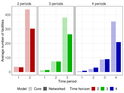
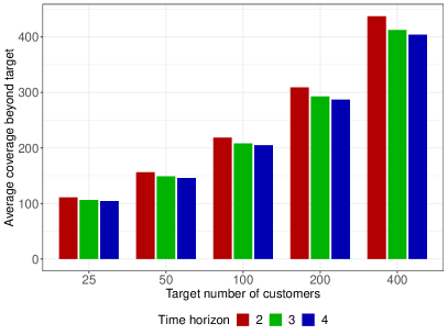
Figure 5(a) reports the average number of facilities that are tentatively opened at each time period under the networked model (Algorithms 34); for comparative purposes, it also shows the solution of the core model in the corresponding setting (Algorithm 1). As expected, fewer facilities need to be opened in the networked setting because each facility can cover multiple customers. Perhaps more surprisingly, a similar number of facilities get tentatively opened in earlier iterations between the two solutions. This observation highlights the distinct roles of exploration and exploitation in the presence of irreversible decisions. In early iterations, the exploration objective is to mitigate the learning error, so the decisions barely depend on the fact that each facility is connected to several customers—recall, also, that the facilities with the smallest expected incremental coverage get selected in early time periods (Proposition 4.6). In later iterations, the exploitation objective is to satisfy the target coverage once the error gets mitigated, so the decision-maker selects fewer but more central facilities to exploit the network structure.

Figure 5(b) reports the average “customer-based regret” at the end of the planning horizon, as a function of $m$ and $T$. Unlike in the core setting, we do not have access to the perfect-information solution, which would involve solving a large-scale binary stochastic optimization problem. We therefore analyze regret in the customer space, as opposed to the facility space. Specifically, we know that the perfect-information solution achieves a coverage of exactly $m$ customers (at worst, within a tolerance of $d_{\star}$), so we report the average customer-based regret as the difference between total customer coverage and the target $m$. Recall that our theoretical results guarantee that Algorithm 2 yields an asymptotically optimal solution and asymptotically tight regret bounds, in $\Theta\left(m^{\frac{1}{2}\cdot\alpha_{T}}\right)$ (this bound extends to customer-based regret since the degree of each node is bounded by $d_{\star}$). The figure shows that the solution obtained with Algorithms 34 also achieves sub-linear regret: as $m$ doubles, the average regret increases by 29% approximately, for all values of $m$ and $T$ under consideration. The $\Theta\left(m^{\frac{1}{2}\cdot\alpha_{T}}\right)$ result would indicate a regret growth by 45% with $T=4$, by 49% with $T=3$, and by 59% with $T=2$. The computational results are therefore consistent with—in fact, slightly better than—the theoretical predictions. Furthermore, the average regret varies only slightly as the planning horizon becomes longer. Altogether, these results confirm our main takeaways regarding the benefits of even limited learning indicated by the sub-linear regret bounds and the exponential convergence of the regret rate as the time horizon increases.

5 Conclusion

Motivated by examples from clinical trials, retail and infrastructure planning, this paper studies an online learning and optimization problem in the presence of irreversible decisions and endogenous supply-side uncertainty. At each period, a decision-maker selects facilities, receives information on the success of each one, and updates a machine learning model to predict facility success. The problem is formulated via multi-stage stochastic optimization to minimize the total number of selected facilities, subject to chance constraints on coverage targets. We leverage statistical learning theory to incorporate a general-purpose characterization of the machine learning model, by assuming that the error rate decays with the inverse square root of the sample size.

Our main result is to derive an asymptotically optimal algorithm and an asymptotically tight bound to show that the regret rate grows sub-linearly as the coverage target grows to infinity—but in a finite and fixed temporal horizon of $T$ periods. We first consider a core setting with a target $m$ on the number of successful facilities, in which we show that the optimal regret grows in $\Theta\left(m^{\frac{1}{2}\cdot\frac{1}{1-2^{-T}}}\right)$. We establish the robustness of this result to the learning error and to the availability of offline data. We then consider a networked setting where each facility is connected to a set of customers, with a target $m$ on the number of customers that are covered by a successful facility. We extend all technical results under time invariance and degree assumptions, again deriving an asymptotically optimal algorithm with an asymptotically tight regret bound in $\Theta\left(m^{\frac{1}{2}\cdot\frac{1}{1-2^{-T}}}\right)$.

These results identify the benefits of learning—in fact, the benefits of limited learning—in online decision-making with irreversible decisions and coverage targets. Specifically, the regret rate grows sub-linearly with the coverage targets, as compared to linearly for a single-period benchmark that does not leverage online learning. Moreover, the regret rate converges exponentially fast as the planning horizon becomes increasingly long, ranging from $\Theta\left(m^{0.67}\right)$ with two periods through $\Theta\left(m^{0.57}\right)$ with three periods and $\Theta\left(m^{0.53}\right)$ with four periods, to $\Theta(\sqrt{m})$ as $T$ grows to infinity. In other words, even a few rounds of learning and optimization can provide strong performance improvements over a no-learning benchmark, by allowing limited exploration initially and enabling more effective exploitation later on as the learning error gets mitigated.

References

  • Agarwal et al. (2019) Agarwal A, Assadi S, Khanna S (2019) Stochastic submodular cover with limited adaptivity. Proceedings of the Thirtieth Annual ACM-SIAM Symposium on Discrete Algorithms, 323–342 (SIAM).
  • Agarwal and Balkanski (2023) Agarwal A, Balkanski E (2023) Learning-augmented dynamic submodular maximization. arXiv preprint arXiv:2311.13006 .
  • Aktaş et al. (2013) Aktaş E, Özaydın Ö, Bozkaya B, Ülengin F, Önsel Ş (2013) Optimizing fire station locations for the istanbul metropolitan municipality. Interfaces 43(3):240–255.
  • Almanza et al. (2021) Almanza M, Chierichetti F, Lattanzi S, Panconesi A, Re G (2021) Online facility location with multiple advice. Advances in Neural Information Processing Systems 34:4661–4673.
  • Anthony et al. (2010) Anthony B, Goyal V, Gupta A, Nagarajan V (2010) A plant location guide for the unsure: Approximation algorithms for min-max location problems. Mathematics of Operations Research 35(1):79–101.
  • Anthony et al. (1999) Anthony M, Bartlett PL, Bartlett PL, et al. (1999) Neural network learning: Theoretical foundations, volume 9 (cambridge university press Cambridge).
  • Arlotto and Gurvich (2019) Arlotto A, Gurvich I (2019) Uniformly bounded regret in the multisecretary problem. Stochastic Systems 9(3):231–260.
  • Auer et al. (2002) Auer P, Cesa-Bianchi N, Freund Y, Schapire RE (2002) The nonstochastic multiarmed bandit problem. SIAM journal on computing 32(1):48–77.
  • Banerjee and Freund (2019) Banerjee S, Freund D (2019) Good prophets know when the end is near. Available at SSRN 3479189 .
  • Bardossy and Raghavan (2010) Bardossy MG, Raghavan S (2010) Dual-based local search for the connected facility location and related problems. INFORMS Journal on Computing 22(4):584–602.
  • Baron et al. (2011) Baron O, Milner J, Naseraldin H (2011) Facility location: A robust optimization approach. Production and Operations Management 20(5):772–785.
  • Baxi et al. (2024) Baxi S, Cummings K, Jacquillat A, McDonald R, Mellou K, Menache I, Molinaro M (2024) Online rack placement in large-scale data centers. Working paper .
  • Bayram and Yaman (2018) Bayram V, Yaman H (2018) Shelter location and evacuation route assignment under uncertainty: A benders decomposition approach. Transportation science 52(2):416–436.
  • Bertsimas et al. (2022) Bertsimas D, Digalakis Jr V, Jacquillat A, Li ML, Previero A (2022) Where to locate covid-19 mass vaccination facilities? Naval Research Logistics (NRL) 69(2):179–200.
  • Boucheron et al. (2005) Boucheron S, Bousquet O, Lugosi G (2005) Theory of classification: A survey of some recent advances. ESAIM: probability and statistics 9:323–375.
  • Bousquet and Elisseeff (2002) Bousquet O, Elisseeff A (2002) Stability and generalization. The Journal of Machine Learning Research 2:499–526.
  • Brøgger-Mikkelsen et al. (2022) Brøgger-Mikkelsen M, Zibert JR, Andersen AD, Lassen U, Hædersdal M, Ali Z, Thomsen SF (2022) Changes in key recruitment performance metrics from 2008–2019 in industry-sponsored phase III clinical trials registered at ClinicalTrials.gov. Plos one 17(7):e0271819.
  • Brooks (1941) Brooks RL (1941) On colouring the nodes of a network. Mathematical Proceedings of the Cambridge Philosophical Society, volume 37, 194–197 (Cambridge University Press).
  • Brown and Uru (2024) Brown DB, Uru C (2024) Sequential search with acquisition uncertainty. Management Science .
  • Bumpensanti and Wang (2020) Bumpensanti P, Wang H (2020) A re-solving heuristic with uniformly bounded loss for network revenue management. Management Science 66(7):2993–3009.
  • Cao et al. (2021) Cao J, Qi W, Zhang Y (2021) Online facility location. Available at SSRN 3930617 .
  • Carlisle et al. (2015) Carlisle B, Kimmelman J, Ramsay T, MacKinnon N (2015) Unsuccessful trial accrual and human subjects protections: an empirical analysis of recently closed trials. Clinical trials 12(1):77–83.
  • Chan et al. (2018) Chan TC, Shen ZJM, Siddiq A (2018) Robust defibrillator deployment under cardiac arrest location uncertainty via row-and-column generation. Operations Research 66(2):358–379.
  • Chaudhuri and Dasgupta (2014) Chaudhuri K, Dasgupta S (2014) Rates of convergence for nearest neighbor classification. Advances in Neural Information Processing Systems 27.
  • Cheng et al. (2021) Cheng C, Adulyasak Y, Rousseau LM (2021) Robust facility location under disruptions. INFORMS Journal on Optimization 3(3):298–314.
  • Chenreddy and Delage (2024) Chenreddy A, Delage E (2024) End-to-end conditional robust optimization. arXiv preprint arXiv:2403.04670 .
  • Chu et al. (2011) Chu W, Li L, Reyzin L, Schapire R (2011) Contextual bandits with linear payoff functions. Proceedings of the Fourteenth International Conference on Artificial Intelligence and Statistics, 208–214 (JMLR Workshop and Conference Proceedings).
  • Cui et al. (2010) Cui T, Ouyang Y, Shen ZJM (2010) Reliable facility location design under the risk of disruptions. Operations research 58(4-part-1):998–1011.
  • Cygan et al. (2018) Cygan M, Czumaj A, Mucha M, Sankowski P (2018) Online facility location with deletions. arXiv preprint arXiv:1807.03839 .
  • Daskin (1997) Daskin M (1997) Network and discrete location: models, algorithms and applications. Journal of the Operational Research Society 48(7):763–764.
  • Daskin (1983) Daskin MS (1983) A maximum expected covering location model: formulation, properties and heuristic solution. Transportation science 17(1):48–70.
  • Farias and Madan (2011) Farias VF, Madan R (2011) The irrevocable multiarmed bandit problem. Operations Research 59(2):383–399.
  • Feldman and Vondrak (2019) Feldman V, Vondrak J (2019) High probability generalization bounds for uniformly stable algorithms with nearly optimal rate. Conference on Learning Theory, 1270–1279 (PMLR).
  • Fotakis (2008) Fotakis D (2008) On the competitive ratio for online facility location. Algorithmica 50(1):1–57.
  • Fotakis (2011) Fotakis D (2011) Online and incremental algorithms for facility location. ACM SIGACT News 42(1):97–131.
  • Fotakis et al. (2021) Fotakis D, Gergatsouli E, Gouleakis T, Patris N (2021) Learning augmented online facility location. arXiv preprint arXiv:2107.08277 .
  • Gao and Zhou (2020) Gao W, Zhou ZH (2020) Towards convergence rate analysis of random forests for classification. Advances in neural information processing systems 33:9300–9311.
  • Ghuge et al. (2022) Ghuge R, Gupta A, Nagarajan V (2022) The power of adaptivity for stochastic submodular cover. Operations Research .
  • Goemans and Vondrák (2006) Goemans M, Vondrák J (2006) Stochastic covering and adaptivity. Latin American symposium on theoretical informatics, 532–543 (Springer).
  • Guo et al. (2020) Guo X, Kulkarni J, Li S, Xian J (2020) On the facility location problem in online and dynamic models. Approximation, Randomization, and Combinatorial Optimization. Algorithms and Techniques (APPROX/RANDOM 2020) (Schloss Dagstuhl-Leibniz-Zentrum für Informatik).
  • Jacquillat et al. (2024) Jacquillat A, Li ML, Ramé M, Wang K (2024) Branch-and-price for prescriptive contagion analytics. Operations Research .
  • Janson (2004) Janson S (2004) Large deviations for sums of partly dependent random variables. Random Structures & Algorithms 24(3):234–248.
  • Jasin and Kumar (2012) Jasin S, Kumar S (2012) A re-solving heuristic with bounded revenue loss for network revenue management with customer choice. Mathematics of Operations Research 37(2):313–345.
  • Jiang et al. (2021) Jiang SHC, Liu E, Lyu Y, Tang ZG, Zhang Y (2021) Online facility location with predictions. arXiv preprint arXiv:2110.08840 .
  • Jin and Ma (2022) Jin B, Ma W (2022) Online bipartite matching with advice: Tight robustness-consistency tradeoffs for the two-stage model. Advances in Neural Information Processing Systems 35:14555–14567.
  • Jin et al. (2018) Jin C, Netrapalli P, Jordan MI (2018) Accelerated gradient descent escapes saddle points faster than gradient descent. Conference On Learning Theory, 1042–1085 (PMLR).
  • Johnson (2015) Johnson O (2015) An evidence-based approach to conducting clinical trial feasibility assessments. Clinical Investigation 5(5):491–499.
  • Kaplan et al. (2023) Kaplan H, Naori D, Raz D (2023) Almost tight bounds for online facility location in the random-order model. Proceedings of the 2023 Annual ACM-SIAM Symposium on Discrete Algorithms (SODA), 1523–1544 (SIAM).
  • Langford and Zhang (2007) Langford J, Zhang T (2007) The epoch-greedy algorithm for contextual multi-armed bandits. Advances in neural information processing systems 20(1):96–1.
  • Laporte et al. (1994) Laporte G, Louveaux FV, van Hamme L (1994) Exact solution to a location problem with stochastic demands. Transportation science 28(2):95–103.
  • Lattanzi et al. (2020a) Lattanzi S, Lavastida T, Moseley B, Vassilvitskii S (2020a) Online scheduling via learned weights. Proceedings of the Fourteenth Annual ACM-SIAM Symposium on Discrete Algorithms, 1859–1877 (SIAM).
  • Lattanzi et al. (2020b) Lattanzi S, Mitrović S, Norouzi-Fard A, Tarnawski JM, Zadimoghaddam M (2020b) Fully dynamic algorithm for constrained submodular optimization. Advances in Neural Information Processing Systems 33:12923–12933.
  • Lattimore and Szepesvári (2020) Lattimore T, Szepesvári C (2020) Bandit algorithms (Cambridge University Press).
  • Lavastida et al. (2020) Lavastida T, Moseley B, Ravi R, Xu C (2020) Learnable and instance-robust predictions for online matching, flows and load balancing. arXiv preprint arXiv:2011.11743 .
  • Lim et al. (2013) Lim MK, Bassamboo A, Chopra S, Daskin MS (2013) Facility location decisions with random disruptions and imperfect estimation. Manufacturing & Service Operations Management 15(2):239–249.
  • Lu et al. (2015) Lu M, Ran L, Shen ZJM (2015) Reliable facility location design under uncertain correlated disruptions. Manufacturing & service operations management 17(4):445–455.
  • Lu et al. (2010) Lu T, Pál D, Pál M (2010) Contextual multi-armed bandits. Proceedings of the Thirteenth international conference on Artificial Intelligence and Statistics, 485–492 (JMLR Workshop and Conference Proceedings).
  • Lykouris and Vassilvitskii (2021) Lykouris T, Vassilvitskii S (2021) Competitive caching with machine learned advice. Journal of the ACM (JACM) 68(4):1–25.
  • Mansour and McAllester (2000) Mansour Y, McAllester DA (2000) Generalization bounds for decision trees. COLT, 69–74 (Citeseer).
  • Mazumder and Wang (2024) Mazumder R, Wang H (2024) On the convergence of cart under sufficient impurity decrease condition. Advances in Neural Information Processing Systems 36.
  • McAllester (1998) McAllester DA (1998) Some pac-bayesian theorems. Proceedings of the eleventh annual conference on Computational learning theory, 230–234.
  • Meyerson (2001) Meyerson A (2001) Online facility location. Proceedings 42nd IEEE Symposium on Foundations of Computer Science, 426–431 (IEEE).
  • Monemizadeh (2020) Monemizadeh M (2020) Dynamic submodular maximization. Advances in Neural Information Processing Systems 33:9806–9817.
  • Ng and Jordan (2001) Ng A, Jordan M (2001) On discriminative vs. generative classifiers: A comparison of logistic regression and naive bayes. Advances in neural information processing systems 14.
  • Osband et al. (2019) Osband I, Van Roy B, Russo DJ, Wen Z (2019) Deep exploration via randomized value functions. Journal of Machine Learning Research 20(124):1–62.
  • Pacala et al. (2021) Pacala S, Cunliff C, Deane-Ryan D, Gallagher K, Haggerty J, Hendrickson C, Jenkins J, Johnson R, Lieuwen T, Loftness V, Miller C, Pizer W, Rai V, Rightor E, Takeuchi E, Tierney S, Wilcox J (2021) Accelerating decarbonization of the us energy system. Technical report, National Academies of Sciences, Engineering, and Medicine.
  • Pollard (2012) Pollard D (2012) Convergence of stochastic processes (Springer Science & Business Media).
  • Powell (2022) Powell W (2022) Reinforcement Learning and Stochastic Optimization: A unified framework for sequential decisions (Hoboken: John Wiley and Sons).
  • Qi et al. (2015) Qi W, Liang Y, Shen ZJM (2015) Joint planning of energy storage and transmission for wind energy generation. Operations Research 63(6):1280–1293.
  • Ročková and Saha (2019) Ročková V, Saha E (2019) On theory for bart. The 22nd international conference on artificial intelligence and statistics, 2839–2848 (PMLR).
  • Russo and Van Roy (2018) Russo D, Van Roy B (2018) Learning to optimize via information-directed sampling. Operations Research 66(1):230–252.
  • Ryzhov et al. (2012) Ryzhov IO, Powell WB, Frazier PI (2012) The knowledge gradient algorithm for a general class of online learning problems. Operations Research 60(1):180–195.
  • Sakhrani (2015) Sakhrani VA (2015) Negotiated collaboration: a study in flexible infrastructure design. Ph.D. thesis, Massachusetts Institute of Technology.
  • Shen et al. (2011) Shen ZJM, Zhan RL, Zhang J (2011) The reliable facility location problem: Formulations, heuristics, and approximation algorithms. INFORMS Journal on Computing 23(3):470–482.
  • Slivkins (2011) Slivkins A (2011) Contextual bandits with similarity information. Proceedings of the 24th annual Conference On Learning Theory, 679–702 (JMLR Workshop and Conference Proceedings).
  • Slivkins et al. (2019) Slivkins A, et al. (2019) Introduction to multi-armed bandits. Foundations and Trends® in Machine Learning 12(1-2):1–286.
  • Snyder and Daskin (2005) Snyder LV, Daskin MS (2005) Reliability models for facility location: the expected failure cost case. Transportation science 39(3):400–416.
  • Sridharan et al. (2008) Sridharan K, Shalev-Shwartz S, Srebro N (2008) Fast rates for regularized objectives. Advances in neural information processing systems 21.
  • Taherkhani et al. (2020) Taherkhani G, Alumur SA, Hosseini M (2020) Benders decomposition for the profit maximizing capacitated hub location problem with multiple demand classes. Transportation Science 54(6):1446–1470.
  • University of California at Irvine (2020) (UCI) University of California at Irvine (UCI) (2020) UC Irvine machine learning repository. Available at http://archive.ics.uci.edu/ml.
  • Uryasev and Rockafellar (2001) Uryasev S, Rockafellar RT (2001) Conditional value-at-risk: optimization approach. Stochastic optimization: algorithms and applications 411–435.
  • Uryasev et al. (2010) Uryasev S, Sarykalin S, Serraino G, Kalinchenko K (2010) Var vs cvar in risk management and optimization. CARISMA conference.
  • Vapnik and Chervonenkis (2015) Vapnik VN, Chervonenkis AY (2015) On the uniform convergence of relative frequencies of events to their probabilities. Measures of complexity: festschrift for alexey chervonenkis, 11–30 (Springer).
  • Vera and Banerjee (2021) Vera A, Banerjee S (2021) The bayesian prophet: A low-regret framework for online decision making. Management Science 67(3):1368–1391.
  • Wang et al. (2024) Wang I, Becker C, Van Parys B, Stellato B (2024) Learning decision-focused uncertainty sets in robust optimization. arXiv e-prints:2305.19225 .
  • Wang et al. (2023) Wang K, Aydemir M, Jacquillat A (2023) Scenario-based robust optimization for two-stage decision making under binary uncertainty. INFORMS Journal on Optimization .
  • Xu and Mannor (2012) Xu H, Mannor S (2012) Robustness and generalization. Machine learning 86:391–423.
\ECSwitch\ECHead

Learning to cover: online learning and optimization with irreversible decisions toward target coverage
Electronic Companion

6 Empirical evidence of the learning function

This appendix reports numerical evidence of the improvement in predictive performance as a function of the sample size. We consider five publicly available datasets from the University of California at Irvine (2020) (UCI) featuring binary classification with multivariate data, 10–100 attributes, more than 1,000 records, and structured data—namely, the datasets called “bank marketing” (“bank”), “default of credit card clients” (“default”), “electrical grid stability” (“electrical”), “occupancy detection” (“occupancy”) and “online shoppers purchasing intention” (“online”). Table 2 reports descriptive statistics of each dataset. The variability in the positive rates indicates different learning tasks and different learning difficulty.

For each sample size, we select ten random subsets of each dataset and, for each one, we run a random forest classification model. Figure 6 plots the classification error as a function of the sample size, averaged across the ten instances. Table 2 and Figure 6 also report the best fits of the form $\frac{\gamma}{\sqrt{n}}+\beta$ (which corresponds to Assumption 1) and of the form $\frac{\gamma}{n^{r}}+\beta$ (which corresponds to the more general learning rates considered in Section 3.4). These results suggest a clear downward trend as the sample size increases, as well as a concave dependency indicating diminishing returns as the sample size becomes increasingly large. The fitted curves yield a good first-order approximation of the learning error, so that the assumption that the learning error decays in $\mathcal{O}(1/\sqrt{n})$ or in $\mathcal{O}(1/n^{r})$ characterizes fairly well the impact of additional data points on predictive performance. Ultimately, these results provide an empirical justification of the general-purpose characterization of the machine learning model in our theoretical analysis.

Table 2: Descriptive statistics of the 10 datasets and corresponding data-driven experimental setup.
Dataset Positive class # observations # features Positive rate Best fit Best fit ($r=0.5$)
Bank 521 4,521 16 11.5% $\frac{0.3}{n^{0.097}}$ $\frac{0.27}{\sqrt{n}}+0.16$
Default 6,636 30,000 23 22.1% $\frac{0.50}{n^{0.68}}+0.18$ $\frac{0.68}{\sqrt{n}}+0.16$
Electric 3,620 10,000 12 36.2% $\frac{1}{n}$ $\frac{0.12}{\sqrt{n}}+0.16$
Occupancy 2,049 9,752 6 21.0% $\frac{0.36}{n^{0.149}}$ $\frac{0.44}{\sqrt{n}}+0.13$
Online 1,908 12,330 6 15.5% $\frac{0.19}{n^{0.085}}$ $\frac{0.15}{\sqrt{n}}+0.11$
Refer to caption
(a)
Refer to caption
(b)
Refer to caption
(c)
Refer to caption
(d)
Refer to caption
(e)
Figure 6: Average error of the classification models as a function of the sample size. The red curve shows the best fit of the form $\frac{\gamma}{n^{r}}+\beta$, and the blue curve shows the best fit of the form $\frac{\gamma}{\sqrt{n}}+\beta$.

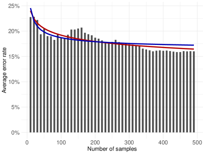
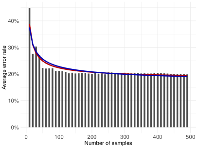
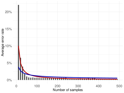
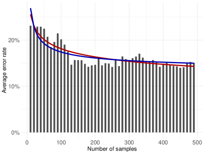
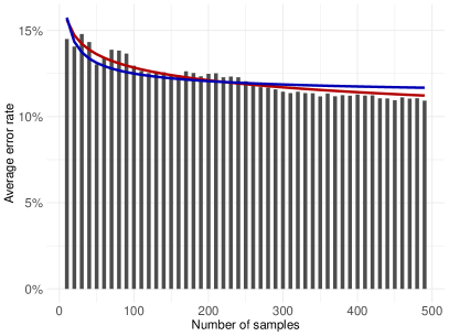
7 Proof of statements from Section 3

Throughout this proof, we denote by $A^{*}_{t}$ the optimal solution of the stochastic problem (Problem ($\mathcal{P}^{*}$)), by $A^{\dagger}_{t}$ the solution given by Algorithm 1, and by $A^{\textsc{D}}_{t}$ the solution of the deterministic approximation (Problem ($\mathcal{P}^{D}$)). We denote by $B^{*}_{t}$, $B^{\dagger}_{t}$, and $B^{\textsc{D}}_{t}$ the corresponding numbers of facilities successfully opened at period $t$, and by $N^{*}_{t}$, $N^{\dagger}_{t}$, and $N^{\textsc{D}}_{t}$ the corresponding coverage variables (i.e., the number of facilities successfully opened by period $t$). The optimal values are denoted as $m^{*}(\varepsilon,T)=\sum_{t=1}^{T}A^{*}_{t}$, $m^{\dagger}(\varepsilon,T)=\sum_{t=1}^{T}A^{\dagger}_{t}$, and $m^{\textsc{D}}(\varepsilon,T)=\sum_{t=1}^{T}A^{\textsc{D}}_{t}$.

With these notations, Lemma 3.3 elicits the solution $A^{\textsc{D}}_{t}$; Lemma 3.5 establishes the feasibility of solution $A^{*}_{t}$ in view of the chance constraint, thus providing a constructive upper bound of $m^{\dagger}(\varepsilon,T)$; and Lemma 3.6 provides a lower bound of $m^{\dagger}(\varepsilon,T)$.

7.1 Proof of Lemma 3.3

Note that the constraint $N^{D}_{T}\geq m$ is binding at optimality, so the problem can be re-written as:

$\displaystyle\min\ \left\{\ \sum_{t=1}^{T}A^{D}_{t}\ \ \bigg{|}\ \ \sum_{t=1}^{T}A^{D}_{t}\left(1-\frac{\varepsilon}{\sqrt{\sum_{s=1}^{t-1}A^{D}_{s}+1}}\ \right)=m\right\}$

Let $\lambda\in\mathbb{R}$ be the dual variable associated with the equality constraint. The Karush–Kuhn–Tucker (KKT) conditions yield the following vanishing gradient equation:

$$1+\lambda\left(1-\frac{\varepsilon}{\sqrt{\sum_{s=1}^{t-1}A^{D}_{s}+1}}\right)+\lambda\sum_{\tau=t+1}^{T}\frac{\varepsilon A^{D}_{\tau}}{2\left(\sum_{s=1}^{\tau-1}A^{D}_{s}+1\right)^{3/2}}=0,\ \forall t\in\mathcal{T}$$

Clearly, $\lambda\neq 0$. After re-arranging the terms, we obtain:

$$\frac{1}{\sqrt{\sum_{s=1}^{t-1}A^{D}_{s}+1}}-\sum_{\tau=t+1}^{T}\frac{A^{D}_{\tau}}{2\left(\sum_{s=1}^{\tau-1}A^{D}_{s}+1\right)^{3/2}}=\frac{1+\lambda}{\lambda\varepsilon},\ \forall t\in\mathcal{T}$$

Note that this expression is independent of $t$. Therefore, for all $t=1,\cdots,T-1$, we have:

$$\frac{1}{\sqrt{\sum_{s=1}^{t-1}A^{D}_{s}+1}}-\sum_{\tau=t+1}^{T}\frac{A^{D}_{\tau}}{2\left(\sum_{s=1}^{\tau-1}A^{D}_{s}+1\right)^{3/2}}=\frac{1}{\sqrt{\sum_{s=1}^{t}A^{D}_{s}+1}}-\sum_{\tau=t+2}^{T}\frac{A^{D}_{\tau}}{2\left(\sum_{s=1}^{\tau-1}A^{D}_{s}+1\right)^{3/2}}.$$

This system of equations gives rise to a simple recurrence relation for $A^{D}_{t}$:

$$A^{D}_{t+1}=\frac{2\left(\sum_{s=1}^{t}A^{D}_{s}+1\right)^{3/2}}{\sqrt{\sum_{s=1}^{t-1}A^{D}_{s}+1}}-2\left(\sum_{s=1}^{t}A^{D}_{s}+1\right),\ \forall t=1,\cdots,T-1.$$

Let us define $u_{t}=\sum_{s=1}^{t}A^{D}_{s}+1$. By expressing $A^{D}_{t}=u_{t}-u_{t-1}$, we can re-write the recursion as:

$$u_{t+1}-u_{t}=\frac{2u_{t}^{3/2}}{\sqrt{u_{t-1}}}-2u_{t},\ \forall t=1,\cdots,T-1,$$

i.e., as:

$$u_{t+1}+u_{t}=\frac{2u_{t}^{3/2}}{\sqrt{u_{t-1}}},\ \forall t=1,\cdots,T-1.$$ (11)

We are interested in the behavior of $u_{t}$ as $m\to\infty$. We perform a leading-order analysis and a leading-coefficient analysis, assuming that $u_{t}=\Theta(g(t)m^{f(t)})$. Note, first, that the boundary condition of $u_{0}=1=\Theta(1)$ implies that $g(0)=1$ and $f(0)=0$. Moreover, we prove below that $u_{T}=m+o(m)=\Theta(m)$, so that $g(T)=1$ and $f(T)=1$.

To see that $u_{T}=m+o(m)=\Theta(m)$, note that the solution $\bar{A}_{1}=\frac{m^{2/3}}{1-\varepsilon}$ and $\bar{A}_{2}=m$ is feasible for Problem ($\mathcal{P}^{D}$) with $T=2$:

$\displaystyle N^{D}_{2}$ $\displaystyle=\bar{A}_{1}(1-\varepsilon)+\bar{A}_{2}\left(1-\frac{\varepsilon}{\sqrt{\bar{A}_{1}+1}}\right)$
$\displaystyle=m^{2/3}+m\left(1-\frac{\varepsilon}{\sqrt{\bar{A}_{1}+1}}\right)$
$\displaystyle\geq m^{2/3}+m-\varepsilon m^{2/3}$
$\displaystyle\geq m$

Therefore, $\left(\frac{m^{2/3}}{1-\varepsilon},m,0,\cdots,0\right)$ is a feasible solution of Problem ($\mathcal{P}^{D}$) with $T\geq 2$, so

$$m+1\leq u_{T}\leq m+\frac{m^{2/3}}{1-\varepsilon}+1$$

This proves that $u_{T}=m+o(m)=\Theta(m)$, hence $g(T)=1$ and $f(T)=1$.

Let us derive the expression of $f(t)$. From Equation (11), we obtain the following recursion:

$$f(t+1)=\frac{3}{2}f(t)-\frac{1}{2}f(t-1),$$

i.e.:

$$f(t+1)-f(t)=\frac{1}{2}\left(f(t)-f(t-1)\right).$$

We derive:

$$f(t+1)-f(t)=\frac{K}{2^{t}},\quad\text{where $K=f(1)-f(0)=f(1)$.}$$

By summation and by telescoping the sum, this yields:

$$\sum_{s=0}^{T-1}(f(s+1)-f(s))=f(T)-f(0)=2K\left(1-\frac{1}{2^{T}}\right).$$

From the boundary conditions, we have $f(T)-f(0)=1$, so that:

$$f(t+1)-f(t)=\frac{1}{2^{t+1}}\cdot\frac{1}{1-\frac{1}{2^{T}}}$$

Again, by summation and by telescoping the sum, the following holds:

$$f(t)=\sum_{s=0}^{t-1}(f(s+1)-f(s))=\frac{1}{1-\frac{1}{2^{T}}}\sum_{s=1}^{t}\frac{1}{2^{s}}=\frac{1-\frac{1}{2^{t}}}{1-\frac{1}{2^{T}}}.$$

In conclusion, the leading-order analysis leads to:

$$u_{t}=\Theta\left(m^{\frac{1-\frac{1}{2^{t}}}{1-\frac{1}{2^{T}}}}\right)=\Theta\left(m^{\alpha_{T}\left(1-\frac{1}{2^{t}}\right)}\right).$$

We conduct a similar analysis for the leading coefficient of $u_{t}$. Equation (11) yields the following recursion:

$$g(t+1)=\frac{2g(t)^{3/2}}{\sqrt{g(t-1)}}$$

Define $h(t)=\log g(t)$ and we have the following modified recurrent relation with the initial conditions $h(0)=h(T)=0$:

$$h(t+1)-\frac{3}{2}h(t)+\frac{1}{2}h(t-1)=\log(2)$$

We proceed as above, with the added drift term. We derive:

$\displaystyle h(t+1)-h(t)=\frac{1}{2}\left(h(t)-h(t-1)\right)+\log(2)$
$\displaystyle h(t+1)-h(t)=\frac{K}{2^{t}}+\log 2\cdot\sum_{s=0}^{t-1}\frac{1}{2^{s}}=\frac{K^{\prime}}{2^{t}}+2\log 2,\quad\text{where $K=h(1)-h(0)$ and $K^{\prime}=K-2\log 2$.}$
$\displaystyle\sum_{s=0}^{T-1}(h(s+1)-h(s))=\underbrace{h(T)-h(0)}_{=0}=2K^{\prime}\left(1-\frac{1}{2^{T}}\right)+2T\log 2\implies K^{\prime}=-\frac{T\log 2}{1-\frac{1}{2^{T}}}$
$\displaystyle h(t+1)-h(t)=2\log 2-\frac{T\log 2}{1-\frac{1}{2^{T}}}\cdot\frac{1}{2^{t}}$
$\displaystyle h(t)=\sum_{s=0}^{t-1}(h(s+1)-h(s))=2t\log 2-\frac{T\log 2}{1-\frac{1}{2^{T}}}\cdot 2\left(1-\frac{1}{2^{t}}\right)=2\log 2\left(t-T\frac{1-\frac{1}{2^{t}}}{1-\frac{1}{2^{T}}}\right).$

Bringing the two results together, we obtain:

$$u_{t}=4^{\left(t-T\frac{1-\frac{1}{2^{t}}}{1-\frac{1}{2^{T}}}\right)}m^{\frac{1-\frac{1}{2^{t}}}{1-\frac{1}{2^{T}}}}+o\left(m^{\frac{1-\frac{1}{2^{t}}}{1-\frac{1}{2^{T}}}}\right)=4^{t-T\cdot\alpha_{T}\cdot\left(1-\frac{1}{2^{t}}\right)}m^{\alpha_{T}\left(1-\frac{1}{2^{t}}\right)}+o\left(m^{\alpha_{T}\left(1-\frac{1}{2^{t}}\right)}\right)$$ (12)

For ease of the exposition, let us write:

$$u_{t}=4^{\overline{h}(t)}m^{f(t)}+o\left(m^{f(t)}\right)$$ (13)

Note that:

$\displaystyle\overline{h}(t)-\frac{1}{2}\overline{h}(t-1)$ $\displaystyle=\left(t-T\frac{1-\frac{1}{2^{t}}}{1-\frac{1}{2^{T}}}\right)-\frac{1}{2}\left(t-1-T\frac{1-\frac{1}{2^{t-1}}}{1-\frac{1}{2^{T}}}\right)=\frac{1}{2}\left(t+1-\frac{T}{1-\frac{1}{2^{T}}}\right)$ (14)
$\displaystyle f(t)-\frac{1}{2}f(t-1)$ $\displaystyle=\left(\frac{1-\frac{1}{2^{t}}}{1-\frac{1}{2^{T}}}\right)-\frac{1}{2}\left(\frac{1-\frac{1}{2^{t-1}}}{1-\frac{1}{2^{T}}}\right)=\frac{1}{2}\frac{1}{1-\frac{1}{2^{T}}}=\frac{1}{2}\cdot\alpha_{T}$ (15)

We conclude as follows:

$\displaystyle\sum_{t=1}^{T}A^{D}_{t}$ $\displaystyle=m+\sum_{t=1}^{T}\frac{A^{D}_{t}\varepsilon}{\sqrt{\sum_{s=1}^{t-1}A^{D}_{s}+1}}$
$\displaystyle=m+\sum_{t=1}^{T}\frac{\varepsilon(u_{t}-u_{t-1})}{\sqrt{u_{t-1}}}$
$\displaystyle=m+\varepsilon\cdot\sum_{t=1}^{T}4^{\overline{h}(t)-\frac{1}{2}\overline{h}(t-1)}\cdot m^{f(t)-\frac{1}{2}f(t-1)}+o\left(m^{f(t)-\frac{1}{2}f(t-1)}\right)$
=m+εm12αT(t=1T2t)22TαT+o(m12αT)(Equations (14) and (15))absent𝑚𝜀superscript𝑚12subscript𝛼𝑇superscriptsubscript𝑡1𝑇superscript2𝑡2superscript2𝑇subscript𝛼𝑇𝑜superscript𝑚12subscript𝛼𝑇(Equations (14) and (15))\displaystyle=m+\varepsilon\cdot m^{\frac{1}{2}\cdot\alpha_{T}}\cdot\left(\sum_{t=1}^{T}2^{t}\right)\cdot\frac{2}{2^{T\cdot\alpha_{T}}}+o\left(m^{\frac{1}{2}\cdot\alpha_{T}}\right)\ \text{(Equations\leavevmode\nobreak\ \eqref{eq:hbar_rec} and\leavevmode\nobreak\ \eqref{eq:f_rec})}
$\displaystyle=m+\varepsilon\cdot\frac{4(2^{T}-1)}{2^{T\cdot\alpha_{T}}}\cdot m^{\frac{1}{2}\cdot\alpha_{T}}+o\left(m^{\frac{1}{2}\cdot\alpha_{T}}\right)$

The expressions for $A^{D}_{t}$ follow immediately from Equation (13) and the fact that $A^{D}_{t}=u_{t}-u_{t-1}$. This concludes the proof. \Halmos

7.2 Proof of Remark 3.4

Note that, in the left-hand side of Equation (2), the term for $t=T$ is equal to $\ell$. We obtain the upper bound directly as a result:

$$\ell\leq\sum_{t=1}^{T}4^{t-T\cdot\alpha_{T}\cdot\left(1-\frac{1}{2^{t}}\right)}\ell^{\alpha_{T}\cdot\left(1-\frac{1}{2^{t}}\right)}=m+\varepsilon\cdot\frac{4(2^{T}-1)}{2^{T\cdot\alpha_{T}}}m^{\frac{1}{2}\cdot\alpha_{T}}+\sqrt{-\frac{1}{2}\log\frac{\delta}{2}}\sqrt{m}.$$

The lower bound follows from the facts that $\alpha_{T}\cdot\left(1-\frac{1}{2^{t}}\right)\leq 1$ and that $1-\frac{1}{2^{t}}\geq 1/2$:

$\displaystyle\sum_{t=1}^{T}4^{t-T\cdot\alpha_{T}\cdot\left(1-\frac{1}{2^{t}}\right)}\left(\frac{3m}{4}\right)^{\alpha_{T}\cdot\left(1-\frac{1}{2^{t}}\right)}$ $\displaystyle\leq\sum_{t=1}^{T}\frac{4^{t}}{4^{T/2\cdot\alpha_{T}}}\left(\frac{3m}{4}\right)=\frac{1}{4^{T/2\cdot\alpha_{T}}}\cdot\frac{4}{3}(4^{T}-1)\cdot\frac{3m}{4}\leq m\cdot 4^{T\left(1-\frac{\alpha_{T}}{2}\right)}.$

We conclude that $\sum_{t=1}^{T}4^{t-T\cdot\alpha_{T}\cdot\left(1-\frac{1}{2^{t}}\right)}\left(\frac{3m}{4}\right)^{\alpha_{T}\cdot\left(1-\frac{1}{2^{t}}\right)}<m+\varepsilon\cdot\frac{4(2^{T}-1)}{2^{T\cdot\alpha_{T}}}m^{\frac{1}{2}\cdot\alpha_{T}}$ for $m$ large enough, hence than $\ell\geq 3m/4$. \Halmos

7.3 Proof of Lemma 3.5

We use the following lemma:

Lemma 7.1

Let $A^{\dagger}_{t}=4^{t-T\frac{1-2^{-t}}{1-2^{-T}}}\ell^{\frac{2^{T}(1-2^{-t})}{2^{T}-1}}$ with $\ell$ defined in Equation (2). We have:

$\displaystyle\mathbb{E}\left[\sum_{t=1}^{T}B^{\dagger}_{t}\right]\geq m+\sqrt{-\frac{1}{2}\log\frac{\delta}{2}}\sqrt{m}-\varepsilon^{2}\cdot\frac{8(2^{T}-1)}{2^{T\cdot\frac{2^{T}+1}{2^{T}-1}}}\cdot m^{\frac{1}{2^{T}-1}}-\varepsilon\cdot\frac{2}{2^{\frac{T}{2^{T}-1}}}\cdot\sqrt{-\frac{1}{2}\log\frac{\delta}{2}}m^{\frac{1}{2(2^{T}-1)}}.$
Proof 7.2

Proof: By definition of $B_{t}$ and by construction of $A_{t}$, we have:

$\displaystyle\mathbb{E}\left[\sum_{t=1}^{T}B^{\dagger}_{t}\right]$ $\displaystyle=\sum_{t=1}^{T}A^{\dagger}_{t}-\sum_{t=1}^{T}\frac{A^{\dagger}_{t}\varepsilon}{\sqrt{\sum_{s=1}^{t-1}A^{\dagger}_{s}+1}}$
$\displaystyle=\sum_{t=1}^{T}\left(4^{t-T\cdot\alpha_{T}\cdot\left(1-\frac{1}{2^{t}}\right)}\ell^{\alpha_{T}\cdot\left(1-\frac{1}{2^{t}}\right)}\right)-\varepsilon\cdot\sum_{t=1}^{T}\frac{4^{t-T\cdot\alpha_{T}\cdot\left(1-\frac{1}{2^{t}}\right)}\ell^{\alpha_{T}\cdot\left(1-\frac{1}{2^{t}}\right)}}{\sqrt{\sum_{s=1}^{t-1}4^{s-T\cdot\alpha_{T}\cdot\left(1-\frac{1}{2^{s}}\right)}\ell^{\alpha_{T}\cdot\left(1-\frac{1}{2^{s}}\right)}+1}}$
$\displaystyle=m+\varepsilon\cdot\frac{4(2^{T}-1)}{2^{T\cdot\alpha_{T}}}m^{\frac{1}{2}\cdot\alpha_{T}}+\sqrt{-\frac{1}{2}\log\frac{\delta}{2}}\sqrt{m}-\varepsilon\cdot\underbrace{\sum_{t=1}^{T}\frac{4^{t-T\cdot\alpha_{T}\cdot\left(1-\frac{1}{2^{t}}\right)}\ell^{\alpha_{T}\cdot\left(1-\frac{1}{2^{t}}\right)}}{\sqrt{\sum_{s=1}^{t-1}4^{s-T\cdot\alpha_{T}\cdot\left(1-\frac{1}{2^{s}}\right)}\ell^{\alpha_{T}\cdot\left(1-\frac{1}{2^{s}}\right)}+1}}}_{(\star)}$

Note that the function $f(x_{1},\cdots,x_{T})=\sum_{t=1}^{T}\frac{x_{t}}{\sqrt{\sum_{l=1}^{t-1}x_{l}+1}}$ is a increasing in all $x_{t}\geq 0$. In Equation (2), the term of the left-hand side expression associated with $t=T$ is equal to $\ell$. Therefore, the equation provides the following (loose) upper bound of $\ell$:

$$\ell\leq m+\varepsilon\cdot\frac{4(2^{T}-1)}{2^{T\cdot\alpha_{T}}}m^{\frac{1}{2}\cdot\alpha_{T}}+\sqrt{-\frac{1}{2}\log\frac{\delta}{2}}\sqrt{m}$$

We can then bound the starred term as follows:

$\displaystyle(\star)$ $\displaystyle\leq\sum_{t=1}^{T}\frac{4^{t-T\frac{1-2^{-t}}{1-2^{-T}}}\left(m+\varepsilon\cdot\frac{4(2^{T}-1)}{2^{\frac{T}{1-2^{-T}}}}m^{\frac{1}{2}\cdot\alpha_{T}}+\sqrt{-\frac{1}{2}\log\frac{\delta}{2}}\sqrt{m}\right)^{\frac{2^{T}(1-2^{-t})}{2^{T}-1}}}{\sqrt{\sum\limits_{s=1}^{t-1}4^{s-T\frac{1-2^{-s}}{1-2^{-T}}}\left(m+\varepsilon\cdot\frac{4(2^{T}-1)}{2^{\frac{T}{1-2^{-T}}}}m^{\frac{1}{2}\cdot\alpha_{T}}+\sqrt{-\frac{1}{2}\log\frac{\delta}{2}}\sqrt{m}\right)^{\frac{2^{T}(1-2^{-s})}{2^{T}-1}}+1}}$
$\displaystyle\leq\sum_{t=1}^{T}\frac{4^{t-T\frac{1-2^{-t}}{1-2^{-T}}}\left(m+\varepsilon\cdot\frac{4(2^{T}-1)}{2^{\frac{T}{1-2^{-T}}}}m^{\frac{1}{2}\cdot\alpha_{T}}+\sqrt{-\frac{1}{2}\log\frac{\delta}{2}}\sqrt{m}\right)^{\frac{2^{T}(1-2^{-t})}{2^{T}-1}}}{\sqrt{4^{t-1-T\frac{1-2^{-t+1}}{1-2^{-T}}}\left(m+\varepsilon\cdot\frac{4(2^{T}-1)}{2^{\frac{T}{1-2^{-T}}}}m^{\frac{1}{2}\cdot\alpha_{T}}+\sqrt{-\frac{1}{2}\log\frac{\delta}{2}}\sqrt{m}\right)^{\frac{2^{T}(1-2^{-t+1})}{2^{T}-1}}}}$
$\displaystyle=\left(\sum_{t=1}^{T}2^{t}\right)2^{1-\frac{T}{1-2^{-T}}}\left(m+\varepsilon\cdot\frac{4(2^{T}-1)}{2^{\frac{T}{1-2^{-T}}}}m^{\frac{1}{2}\cdot\alpha_{T}}+\sqrt{-\frac{1}{2}\log\frac{\delta}{2}}\sqrt{m}\right)^{\frac{1}{2}\cdot\alpha_{T}}$
$\displaystyle=\frac{4(2^{T}-1)}{2^{\frac{T}{1-2^{-T}}}}m^{\frac{2^{T-1}}{2^{T}-1}}\cdot\left(1+\varepsilon\cdot\frac{4(2^{T}-1)}{2^{\frac{T}{1-2^{-T}}}}m^{\frac{1-2^{T-1}}{2^{T}-1}}+\sqrt{-\frac{1}{2}\log\frac{\delta}{2}}m^{-1/2}\right)^{\frac{1}{2}\cdot\alpha_{T}}$
$\displaystyle\leq\frac{4(2^{T}-1)}{2^{\frac{T}{1-2^{-T}}}}m^{\frac{2^{T-1}}{2^{T}-1}}$
$\displaystyle+\frac{4(2^{T}-1)}{2^{\frac{T}{1-2^{-T}}}}m^{\frac{2^{T-1}}{2^{T}-1}}\cdot\frac{2^{T-1}}{2^{T}-1}\cdot\varepsilon\cdot\frac{4(2^{T}-1)}{2^{\frac{T}{1-2^{-T}}}}m^{\frac{1-2^{T-1}}{2^{T}-1}}$
$\displaystyle+\frac{4(2^{T}-1)}{2^{\frac{T}{1-2^{-T}}}}m^{\frac{2^{T-1}}{2^{T}-1}}\cdot\frac{2^{T-1}}{2^{T}-1}\cdot\sqrt{-\frac{1}{2}\log\frac{\delta}{2}}m^{-1/2}$
$\displaystyle=\frac{4(2^{T}-1)}{2^{\frac{T}{1-2^{-T}}}}m^{\frac{2^{T-1}}{2^{T}-1}}+\frac{8(2^{T}-1)}{2^{T\cdot\frac{2^{T}+1}{2^{T}-1}}}\cdot\varepsilon\cdot m^{\frac{1}{2^{T}-1}}+\frac{2}{2^{\frac{T}{2^{T}-1}}}\cdot\sqrt{-\frac{1}{2}\log\frac{\delta}{2}}m^{\frac{1}{2(2^{T}-1)}}$

where the first inequality comes from the upper bound on $\ell$, the second inequality is obtained by bounding the sum by the term associated with $s=t-1$, the next equality follows from Equations (14) and (15), the next equality follows from algebra, the last inequality stems from the fact that $(1+a)^{\delta}\leq 1+\delta a$, and the last equality follows from re-arranging the terms.

By plugging this bound into the previous equation, we obtain:

$\displaystyle\mathbb{E}\left[\sum_{t=1}^{T}B_{t}\right]$ $\displaystyle\geq m+\varepsilon\cdot\frac{4(2^{T}-1)}{2^{T\cdot\alpha_{T}}}m^{\frac{1}{2}\cdot\alpha_{T}}+\sqrt{-\frac{1}{2}\log\frac{\delta}{2}}\sqrt{m}$
$\displaystyle-\varepsilon\cdot\left(\frac{4(2^{T}-1)}{2^{T\cdot\alpha_{T}}}m^{\frac{2^{T-1}}{2^{T}-1}}+\frac{8(2^{T}-1)}{2^{T\cdot\frac{2^{T}+1}{2^{T}-1}}}\cdot\varepsilon\cdot m^{\frac{1}{2^{T}-1}}+\frac{2}{2^{\frac{T}{2^{T}-1}}}\cdot\sqrt{-\frac{1}{2}\log\frac{\delta}{2}}m^{\frac{1}{2(2^{T}-1)}}\right)$
$\displaystyle=m+\sqrt{-\frac{1}{2}\log\frac{\delta}{2}}\sqrt{m}-\varepsilon^{2}\cdot\frac{8(2^{T}-1)}{2^{T\cdot\frac{2^{T}+1}{2^{T}-1}}}\cdot m^{\frac{1}{2^{T}-1}}-\varepsilon\cdot\frac{2}{2^{\frac{T}{2^{T}-1}}}\cdot\sqrt{-\frac{1}{2}\log\frac{\delta}{2}}m^{\frac{1}{2(2^{T}-1)}}$

This completes the proof of Lemma 7.1. \Halmos

Proof of Lemma 3.5.

Note that $0\leq B^{\dagger}_{t}\leq A^{\dagger}_{t}$ for all $t=1,\cdots,T$. By Hoeffding’s inequality, we have:

$\displaystyle\mathbb{P}\left(N^{\dagger}_{T}<m\right)$ $\displaystyle=\mathbb{P}\left(\sum_{t=1}^{T}B^{\dagger}_{t}<m\right)$
$\displaystyle=\mathbb{P}\left(\mathbb{E}\left[\sum_{t=1}^{T}B^{\dagger}_{t}\right]-\sum_{t=1}^{T}B^{\dagger}_{t}<\mathbb{E}\left[\sum_{t=1}^{T}B^{\dagger}_{t}\right]-m\right)$
$\displaystyle\leq\mathbb{P}\left(\left|\sum_{t=1}^{T}B^{\dagger}_{t}-\mathbb{E}\left[\sum_{t=1}^{T}B^{\dagger}_{t}\right]\right|>\left|\mathbb{E}\left[\sum_{t=1}^{T}B^{\dagger}_{t}\right]-m\right|\right)$
$\displaystyle\leq 2\exp\left(-2\frac{\left(\mathbb{E}\left[\sum_{t=1}^{T}B^{\dagger}_{t}\right]-m\right)^{2}}{\sum_{t=1}^{T}A^{\dagger}_{t}}\right)$

By Lemma 7.1 and by construction of $A^{\dagger}_{t}$, this yields:

$\displaystyle\mathbb{P}\left(N^{\dagger}_{T}<m\right)$ $\displaystyle\leq 2\exp\left(-2\frac{\left(\sqrt{-\frac{1}{2}\log\frac{\delta}{2}}\sqrt{m}-\varepsilon^{2}\cdot\frac{8(2^{T}-1)}{2^{T\cdot\frac{2^{T}+1}{2^{T}-1}}}\cdot m^{\frac{1}{2^{T}-1}}-\varepsilon\cdot\frac{2}{2^{\frac{T}{2^{T}-1}}}\cdot\sqrt{-\frac{1}{2}\log\frac{\delta}{2}}m^{\frac{1}{2(2^{T}-1)}}\right)^{2}}{m+\varepsilon\cdot\frac{4(2^{T}-1)}{2^{T\cdot\alpha_{T}}}m^{\frac{1}{2}\cdot\alpha_{T}}+\sqrt{-\frac{1}{2}\log\frac{\delta}{2}}\sqrt{m}}\right)$

By taking the limit as $m$ goes to infinity, we conclude:

$\displaystyle\lim_{m\to\infty}\mathbb{P}\left(N^{\dagger}_{T}<m\right)$ $\displaystyle\leq 2\exp\left(-2\left(\sqrt{-\frac{1}{2}\log\frac{\delta}{2}}\right)^{2}\right)=\delta$

We conclude that $\lim_{m\to\infty}\mathbb{P}\left(N^{\dagger}_{T}\geq m\right)\geq 1-\delta$. \Halmos

7.4 Proof of Lemma 3.6

Let $k$ be a constant such that $\frac{1}{2}<k<\frac{1}{2}\alpha_{T}$. Let us define the following “good” event, for $k>0$:

$$\mathcal{E}_{k}=\left\{\left|B_{t}-A_{t}\left(1-\frac{\varepsilon}{\sqrt{\sum_{s=1}^{t-1}A_{s}+1}}\right)\right|\leq m^{k},\ \forall t\in\{1,\cdots,T\}\right\}$$

We make use of the following two lemmas.

Lemma 7.3

If $A_{t}\leq m+\mathcal{O}(m^{\frac{1}{2}\cdot\alpha_{T}})$ for all $t=1,\cdots,T$, we have, as $m\to\infty$:

$$\mathbb{P}(\mathcal{E}_{k}^{c})=\mathcal{O}(\exp\left(-m^{2k-1}\right))$$
Proof 7.4

Proof: By definition, $B_{t}$ is binomially distributed with parameters $A_{t}$ and $p_{t}=1-\frac{\varepsilon}{\sqrt{\sum_{s=1}^{t-1}A_{s}+1}}$, so $\mathbb{E}[B_{t}]=A_{t}p_{t}$. Hoeffding’s inequality yields, for any $t=1,\cdots,T$:

$\displaystyle\mathbb{P}(|B_{t}-\mathbb{E}[B_{t}]|\geq m^{k})$ $\displaystyle\leq 2\exp\left(-\frac{2m^{2k}}{A_{t}}\right)$
$\displaystyle\leq 2\exp\left(-\frac{2m^{2k}}{m+\mathcal{O}(m^{\frac{1}{2}\cdot\alpha_{T}})}\right)$
$\displaystyle=\mathcal{O}\left(\exp\left(-m^{2k-1}\right)\right)$

By assumption, $2k-1>0$, so $\mathbb{P}\left(|B_{t}-\mathbb{E}[B_{t}]|\geq m^{k}\right)\to 0$ as as $m\to\infty$. Therefore, we obtain from the union bound:

$\displaystyle\mathbb{P}(\mathcal{E}_{k}^{c})$ $\displaystyle=\mathbb{P}\left(\exists t\in\{1,\cdots,T\}\;\;s.t.\;\;\left|B_{t}-A_{t}\left(1-\frac{\varepsilon}{\sqrt{\sum_{s=1}^{t-1}A_{s}+1}}\right)\right|\geq m^{k}\right)$
$\displaystyle\leq\sum_{t=1}^{T}\mathbb{P}\left(\left|B_{t}-A_{t}\left(1-\frac{\varepsilon}{\sqrt{\sum_{s=1}^{t-1}A_{s}+1}}\right)\right|\geq m^{k}\right)$
$\displaystyle=\mathcal{O}(\exp\left(-m^{2k-1}\right))$

This completes the proof of Lemma 7.3. \Halmos

Lemma 7.5

Let $(B^{*}_{1},\cdots,B^{*}_{T})$ denote the optimal solution of Problem ($\mathcal{P}^{*}$). If $\delta=o\left(m^{\frac{1}{2}\cdot\alpha_{T}-1}\right)$, then, we have, as $m\to\infty$:

$\displaystyle\sum_{\sigma=0}^{\infty}\sigma\mathbb{P}\left(\sum_{t=1}^{T}B_{t}^{*}=\sigma\mid\mathcal{E}_{k}\right)$ $\displaystyle\geq m+o\left(m^{\frac{1}{2}\cdot\alpha_{T}}\right)$
$\displaystyle\sum_{\sigma=0}^{\infty}(\sigma-Tm^{k})^{\frac{1}{2}\cdot\alpha_{T}}\mathbb{P}\left(\sum_{t=1}^{T}B_{t}^{*}=\sigma\mid\mathcal{E}_{k}\right)$ $\displaystyle\geq m^{\frac{1}{2}\cdot\alpha_{T}}+o\left(m^{\frac{1}{2}\cdot\alpha_{T}}\right)$
Proof 7.6

Proof: Note that the optimal solution of Problem ($\mathcal{P}^{*}$) must satisfy the constraint:

$$\mathbb{P}\left(\sum_{t=1}^{T}B_{t}^{*}\geq m\right)\geq 1-\delta=1-o\left(m^{\frac{1}{2}\cdot\alpha_{T}-1}\right)$$ (16)

Therefore, we have that:

$\displaystyle\mathbb{P}\left(\sum_{t=1}^{T}B_{t}^{*}\geq m\mid\mathcal{E}_{k}\right)$ $\displaystyle=\frac{\mathbb{P}\left(\sum_{t=1}^{T}B_{t}^{*}\geq m\right)-\mathbb{P}\left(\sum_{t=1}^{T}B_{t}^{*}\geq m\mid\mathcal{E}_{k}^{c}\right)\mathbb{P}(\mathcal{E}_{k}^{c})}{\mathbb{P}(\mathcal{E}_{k})}$
1o(m12αT1)𝒪(exp(m2k1))(Equation (16) and Lemma 7.3)absent1𝑜superscript𝑚12subscript𝛼𝑇1𝒪superscript𝑚2𝑘1(Equation (16) and Lemma 7.3)\displaystyle\geq 1-o\left(m^{\frac{1}{2}\cdot\alpha_{T}-1}\right)-\mathcal{O}\left(\exp\left(-m^{2k-1}\right)\right)\quad\text{(Equation\leavevmode\nobreak\ \eqref{eq:Bmdelta} and Lemma\leavevmode\nobreak\ \ref{lem:hoeffding_bound})}
$\displaystyle=1-o\left(m^{\frac{1}{2}\cdot\alpha_{T}-1}\right)$

Then, we have:

$$\sum_{\sigma=0}^{\infty}\sigma\mathbb{P}\left(\sum_{t=1}^{T}B_{t}^{*}=\sigma\mid\mathcal{E}_{k}\right)\geq m\cdot\mathbb{P}\left(\sum_{t=1}^{T}B_{t}^{*}\geq m\mid\mathcal{E}_{k}\right)\geq m+o\left(m^{\frac{1}{2}\cdot\alpha_{T}}\right)$$

Similarly:

$\displaystyle\sum_{\sigma=0}^{\infty}(\sigma-Tm^{k})^{\frac{1}{2}\cdot\alpha_{T}}\mathbb{P}\left(\sum_{t=1}^{T}B_{t}^{*}=\sigma\mid\mathcal{E}_{k}\right)$
$\displaystyle\geq(m-Tm^{k})^{\frac{1}{2}\cdot\alpha_{T}}\mathbb{P}\left(\sum_{t=1}^{T}B_{t}^{*}\geq m\mid\mathcal{E}_{k}\right)$
$\displaystyle\geq m^{\frac{1}{2}\cdot\alpha_{T}}(1-Tm^{k-1})^{\frac{1}{2}\cdot\alpha_{T}}\left(1-o\left(m^{\frac{1}{2}\cdot\alpha_{T}-1}\right)\right)$
$\displaystyle\geq m^{\frac{1}{2}\cdot\alpha_{T}}\left(1-T^{\frac{1}{2}\cdot\alpha_{T}}m^{(k-1)\frac{1}{2}\cdot\alpha_{T}}+o\left(m^{(k-1)\frac{1}{2}\cdot\alpha_{T}}\right)\right)\left(1-o\left(m^{\frac{1}{2}\cdot\alpha_{T}-1}\right)\right)$
$\displaystyle=m^{\frac{1}{2}\cdot\alpha_{T}}\left(1-T^{\frac{1}{2}\cdot\alpha_{T}}m^{(k-1)\frac{1}{2}\cdot\alpha_{T}}+o\left(m^{\frac{1}{2}\cdot\alpha_{T}-1}\right)\right)$
$\displaystyle=m^{\frac{1}{2}\cdot\alpha_{T}}+o(m^{\frac{1}{2}\cdot\alpha_{T}}),$

where the third inequality follows from Taylor expansion and the last two inequalities follow from the assumption that $k<\frac{1}{2}\alpha_{T}\leq 1$. This completes the proof of Lemma 7.5. \Halmos

Proof of Lemma 3.6.

Let $(A^{*}_{1},\cdots,A^{*}_{T})$ and $(B^{*}_{1},\cdots,B^{*}_{T})$ denote the optimal solution of Problem ($\mathcal{P}^{*}$). We have:

$\displaystyle\mathbb{E}\left[\sum_{t=1}^{T}A^{*}_{t}\right]$ $\displaystyle=\mathbb{E}\left[\sum_{t=1}^{T}A^{*}_{t}\mid\mathcal{E}_{k}\right]\mathbb{P}(\mathcal{E}_{k})+\mathbb{E}\left[\sum_{t=1}^{T}A^{*}_{t}\mid\mathcal{E}_{k}^{c}\right]\mathbb{P}(\mathcal{E}_{k}^{c})$
𝔼[t=1TAtk](1𝒪(exp(m2k1)))(Lemma 7.3)absent𝔼delimited-[]conditionalsuperscriptsubscript𝑡1𝑇subscriptsuperscript𝐴𝑡subscript𝑘1𝒪superscript𝑚2𝑘1(Lemma 7.3)\displaystyle\geq\mathbb{E}\left[\sum_{t=1}^{T}A^{*}_{t}\mid\mathcal{E}_{k}\right]\left(1-\mathcal{O}(\exp(-m^{2k-1}))\right)\quad\text{(Lemma\leavevmode\nobreak\ \ref{lem:hoeffding_bound})}
$\displaystyle=\mathbb{E}\left[\sum_{t=1}^{T}A^{*}_{t}\mid\mathcal{E}_{k}\right]+o(1)$

Conditioned on $\mathcal{E}_{k}$, we have:

$$\sum_{t=1}^{T}B^{*}_{t}=\sum_{t=1}^{T}\mathbb{E}(B^{*}_{t})-\sum_{t=1}^{T}(B^{*}_{t}-\mathbb{E}(B^{*}_{t}))\geq\sum_{t=1}^{T}\mathbb{E}(B^{*}_{t})-\sum_{t=1}^{T}|B^{*}_{t}-\mathbb{E}(B^{*}_{t})|\geq\sum_{t=1}^{T}\mathbb{E}(B^{*}_{t})-Tm^{k}$$

Therefore, the following holds:

$\displaystyle\mathbb{E}\left[\sum_{t=1}^{T}A^{*}_{t}\mid\mathcal{E}_{k}\right]$ $\displaystyle=\sum_{\sigma=0}^{\infty}\mathbb{E}\left[\sum_{t=1}^{T}A^{*}_{t}\mid\mathcal{E}_{k},\sum_{t=1}^{T}B^{*}_{t}=\sigma\right]\mathbb{P}\left(\sum_{t=1}^{T}B^{*}_{t}=\sigma\mid\mathcal{E}_{k}\right)$
$\displaystyle=\sum_{\sigma=0}^{\infty}\mathbb{E}\left[\sum_{t=1}^{T}A^{*}_{t}\mid\mathcal{E}_{k},\sum_{t=1}^{T}B^{*}_{t}=\sigma,\sum_{t=1}^{T}A^{*}_{t}\left(1-\frac{\varepsilon}{\sqrt{\sum_{s=1}^{t-1}A^{*}_{s}+1}}\right)\geq\sigma-Tm^{k}\right]\mathbb{P}\left(\sum_{t=1}^{T}B^{*}_{t}=\sigma\mid\mathcal{E}_{k}\right)$

From Lemma 3.3, we can lower bound the first expression to obtain:

$\displaystyle\mathbb{E}\left[\sum_{t=1}^{T}A^{*}_{t}\mid\mathcal{E}_{k}\right]$
$\displaystyle\geq\sum_{\sigma=0}^{\infty}\left(\sigma-Tm^{k}+\varepsilon\cdot\frac{4(2^{T}-1)}{2^{T\cdot\alpha_{T}}}\cdot(\sigma-Tm^{k})^{\frac{1}{2}\cdot\alpha_{T}}+o\left((\sigma-Tm^{k})^{\frac{1}{2}\cdot\alpha_{T}}\right)\right)\mathbb{P}\left(\sum_{t=1}^{T}B^{*}_{t}=\sigma\mid\mathcal{E}_{k}\right)$
$\displaystyle+o(1)$
$\displaystyle\geq\sum_{\sigma=0}^{\infty}\sigma\mathbb{P}\left(\sum_{t=1}^{T}B^{*}_{t}=\sigma\mid\mathcal{E}_{k}\right)$
$\displaystyle+\varepsilon\cdot\frac{4(2^{T}-1)}{2^{T\cdot\alpha_{T}}}\cdot\sum_{\sigma=0}^{\infty}(\sigma-Tm^{k})^{\frac{1}{2}\cdot\alpha_{T}}\mathbb{P}\left(\sum_{t=1}^{T}B^{*}_{t}=\sigma\mid\mathcal{E}_{k}\right)$
$\displaystyle+o\left(\sum_{\sigma=0}^{\infty}(\sigma-Tm^{k})^{\frac{1}{2}\cdot\alpha_{T}}\mathbb{P}\left(\sum_{t=1}^{T}B^{*}_{t}=\sigma\mid\mathcal{E}_{k}\right)\right)$
$\displaystyle+o(m^{k})$

Per Lemma 7.5, we conclude that:

$\displaystyle\mathbb{E}\left[\sum_{t=1}^{T}A^{*}_{t}\mid\mathcal{E}_{k}\right]$ $\displaystyle\geq m+\varepsilon\cdot\frac{4(2^{T}-1)}{2^{T\cdot\alpha_{T}}}m^{\frac{1}{2}\cdot\alpha_{T}}+o\left(m^{\frac{1}{2}\cdot\alpha_{T}}\right),$

because $k<\frac{1}{2}\alpha_{T}$. The proof is completed since $\mathbb{E}\left[\sum_{t=1}^{T}A^{*}_{t}\right]\geq\mathbb{E}\left[\sum_{t=1}^{T}A^{*}_{t}\mid\mathcal{E}_{k}\right]+o(1)$. \Halmos

7.5 Proof of Theorem 3.1

The main result follows directly from the lemmas. Per Lemma 3.5, the solution given in Algorithm 1 is feasible in Problem ($\mathcal{P}^{*}$). Per Equations (1) and (2), it achieves an upper bound of:

$$m+\varepsilon\cdot\frac{4(2^{T}-1)}{2^{T\cdot\alpha_{T}}}m^{\frac{1}{2}\cdot\alpha_{T}}+\sqrt{-\frac{1}{2}\log\frac{\delta}{2}}\sqrt{m}=m+\varepsilon\cdot\frac{4(2^{T}-1)}{2^{T\cdot\alpha_{T}}}m^{\frac{1}{2}\cdot\alpha_{T}}+o\left(m^{\frac{1}{2}\cdot\alpha_{T}}\right),$$

because $\alpha_{T}>1$. Moreover, per Lemma 3.6, we know that the optimal solution of Problem ($\mathcal{P}^{*}$) admits a lower bound of

$$m+\varepsilon\cdot\frac{4(2^{T}-1)}{2^{T\cdot\alpha_{T}}}m^{\frac{1}{2}\cdot\alpha_{T}}+o\left(m^{\frac{1}{2}\cdot\alpha_{T}}\right).$$

This completes the proof. \Halmos

7.6 Proof of Theorem 3.7

Let us outline the stochastic problem $(\mathcal{P}^{*}_{r})$, the solution of our algorithm (referred to as $(\mathcal{P}^{\dagger}_{r})$), and the deterministic approximation (referred to as $(\mathcal{P}^{D}_{r})$):

  • Stochastic problem: it is identical to Problem ($\mathcal{P}^{*}$), except for the definition of $B_{t}$:

    $\displaystyle\min\quad$ $\displaystyle\sum_{t=1}^{T}A_{t}$ ($\mathcal{P}^{*}_{r}$)
    s.t. $\displaystyle\mathbb{P}\left[\left[\sum_{t=1}^{T}B_{t}\geq m\right]\right]\geq 1-\delta$
    $\displaystyle B_{t}\sim\operatorname{Bino}\left(A_{t},1-\frac{\varepsilon}{\left(\sum_{s=1}^{t-1}A_{s}+1\right)^{r}}\right),\ \forall t\in\mathcal{T}$
    At,Bt0,t𝒯formulae-sequencesubscript𝐴𝑡subscript𝐵𝑡0for-all𝑡𝒯\displaystyle A_{t},B_{t}\geq 0,\ \forall t\in\mathcal{T}
  • Deterministic approximation: it is formulated as Problem ($\mathcal{P}^{D}$) with the same modifications:

    $\displaystyle\min\ \left\{\ \sum_{t=1}^{T}A^{D}_{t}\ \ \bigg{|}\ \ \sum_{t=1}^{T}A^{D}_{t}\left(1-\frac{\varepsilon}{\left(\sum_{s=1}^{t-1}A^{D}_{s}+1\right)^{r}}\right)=m\right\}$ ($\mathcal{P}^{D}_{r}$)
  • Algorithm: our solution is similar to the one from Algorithm 1, except that the number of facilities tentatively opened is adjusted to account for the difference in the learning rate:

    $$A^{\dagger}_{t}=\begin{cases}\left(\frac{1}{r}\right)^{\frac{1}{1-r}\left(t-T\frac{1-r^{t}}{1-r^{T}}\right)}\cdot\ell^{\frac{1-r^{t}}{1-r^{T}}}&\text{if $r\neq 1$}\\ \ell^{t/T}&\text{if $r=1$}\end{cases}$$ (17)

    where $\ell$ is now defined as the unique positive solution to the following equation:

    $\displaystyle\begin{cases}\sum_{t=1}^{T}\left(\frac{1}{r}\right)^{\frac{1}{1-r}\left(t-T\frac{1-r^{t}}{1-r^{T}}\right)}\cdot\ell^{\frac{1-r^{t}}{1-r^{T}}}=m+\varepsilon\cdot\frac{1}{1-r}\left(\frac{1}{r^{T}}-1\right)\frac{\left(\frac{1}{r}\right)^{\frac{r}{1-r}}}{\left(\frac{1}{r}\right)^{T\cdot\frac{1}{1-r^{t}}}}\cdot m^{\frac{1-r}{1-r^{T}}}+\sqrt{-\frac{1}{2}\log\frac{\delta}{2}}\sqrt{m}&\text{if $r\neq 1$}\\ \sum_{t=1}^{T}\ell^{t/T}=m+\varepsilon\cdot m^{1/T}+\sqrt{-\frac{1}{2}\log\frac{\delta}{2}}\sqrt{m}.\qquad(r=1)&\text{if $r=1$}\end{cases}$

The proof of the theorem is mechanistically the same as the proof of Theorem 3.1. The only non-trivial change comes from calculating the optimal solution for Problem ($\mathcal{P}^{D}_{r}$) (i.e. the equivalent of Lemma 3.3). We proceed to state and prove this result.

Lemma 7.7 (Asymptotic solution of Problem ($\mathcal{P}^{D}_{r}$))

Let $m^{D}(\varepsilon,T)$ be the optimal objective value of Problem ($\mathcal{P}^{D}_{r}$), and $A^{D}_{1},\cdots,A^{D}_{T}$ be its solution. For any $T\geq 2$, we have as $m\to\infty$:

$\displaystyle A^{D}_{t}=\begin{cases}\left(\frac{1}{r}\right)^{\frac{1}{1-r}\left(t-T\frac{1-r^{t}}{1-r^{T}}\right)}\cdot m^{\frac{1-r^{t}}{1-r^{T}}}+o\left(m^{\frac{1-r^{t}}{1-r^{T}}}\right)&\text{if $r\neq 1$}\\ m^{\frac{t}{T}}+o\left(m^{\frac{t}{T}}\right)&\text{if $r=1$}\end{cases}$
$\displaystyle m^{D}(\varepsilon,T)=\begin{cases}m+\varepsilon\cdot\frac{1}{1-r}\left(\frac{1}{r^{T}}-1\right)\frac{\left(\frac{1}{r}\right)^{\frac{r}{1-r}}}{\left(\frac{1}{r}\right)^{T\cdot\frac{1}{1-r^{t}}}}\cdot m^{\frac{1-r}{1-r^{T}}}+o\left(m^{\frac{1-r}{1-r^{T}}}\right)&\text{if $r\neq 1$}\\ m+\varepsilon\cdot m^{1/T}+o\left(m^{1/T}\right)&\text{if $r=1$}\end{cases}.$
Proof 7.8

Proof: Let $\lambda\in\mathbb{R}$ be the dual variable associated with the equality constraint. The KKT conditions yield the following vanishing gradient equation:

$$1+\lambda\left(1-\frac{\varepsilon}{\left(\sum_{s=1}^{t-1}A^{D}_{s}+1\right)^{r}}\right)+\lambda\sum_{\tau=t+1}^{T}\frac{\varepsilon rA^{D}_{\tau}}{\left(\sum_{s=1}^{\tau-1}A^{D}_{s}+1\right)^{r+1}}=0,\ \forall t\in\mathcal{T}$$

As in the proof of Lemma 3.3, we define $u_{t}=\sum_{s=1}^{t}A^{D}_{s}+1$ and obtain the following recursion:

$$ru_{t+1}=(r-1)u_{t}+\frac{u_{t}^{r+1}}{u_{t-1}^{r}},\ \forall t=1,\cdots,T-1.$$

Let us write $u_{t}=\Theta(g(t)m^{f(t)})$ toward our leading-order and leading-coefficient analyses. Recall the boundary conditions of $g(0)=1$, $f(0)=0$, $g(T)=1$ and $f(T)=1$. We separate two cases:

Case 1: $\bm{r\neq 1}$

Proceeding as in the proof of Lemma 3.3, we write:

$$f(t+1)=(r+1)f(t)-rf(t-1),$$

and obtain:

$$f(t)=\frac{1-r^{t}}{1-r^{T}}.$$

Similarly, we write:

$$rg(t+1)=\frac{g(t)^{r+1}}{g(t-1)^{r}},$$

With $h(t)=\log g(t)$, we have $h(0)=h(T)=0$ and:

$$h(t+1)=(r+1)h(t)-rh(t-1)-\log r$$

Proceeding again as in the proof of Lemma 3.3, we obtain:

$$h(t)=-\frac{\log r}{1-r}\left(t-T\frac{1-r^{t}}{1-r^{T}}\right).$$

Bringing the two results together, we obtain:

$$u_{t}=\left(\frac{1}{r}\right)^{\frac{1}{1-r}\left(t-T\frac{1-r^{t}}{1-r^{T}}\right)}\cdot m^{\frac{1-r^{t}}{1-r^{T}}}+o\left(m^{\frac{1-r^{t}}{1-r^{T}}}\right).$$

We conclude as follows:

$\displaystyle\sum_{t=1}^{T}A^{D}_{t}$ $\displaystyle=m+\sum_{t=1}^{T}\frac{A^{D}_{t}\varepsilon}{\left(\sum_{s=1}^{t-1}A^{D}_{s}+1\right)^{r}}$
$\displaystyle=m+\sum_{t=1}^{T}\frac{\varepsilon(u_{t}-u_{t-1})}{u_{t-1}^{r}}$
$\displaystyle=m+\varepsilon\cdot\left(\frac{1}{r}\right)^{\frac{r}{1-r}-\frac{T}{1-r^{T}}}\cdot\left(\sum_{t=1}^{T}\frac{1}{r^{t}}\right)m^{\frac{1-r}{1-r^{T}}}+o\left(m^{\frac{1-r}{1-r^{T}}}\right)$
$\displaystyle=m+\varepsilon\cdot\frac{1}{1-r}\left(\frac{1}{r^{T}}-1\right)\frac{\left(\frac{1}{r}\right)^{\frac{r}{1-r}}}{\left(\frac{1}{r}\right)^{T\cdot\frac{1}{1-r^{t}}}}\cdot m^{\frac{1-r}{1-r^{T}}}+o\left(m^{\frac{1-r}{1-r^{T}}}\right).$

Case 2: $\bm{r=1}$ The recursion reduces to:

$$u_{t+1}=\frac{u_{t}^{2}}{u_{t-1}},\ \forall t=1,\cdots,T-1.$$

The leading-order analysis indicates that $f(t+1)-f(t)$ is constant. Since $f(T)-f(0)=1$, we have $f(t+1)-f(t)=1/T$, hence $f(t)=t/T$ for all $t=1,\cdots,T$.

Turning to the leading-coefficient analysis, we write:

$$g(t+1)=\frac{g(t)^{2}}{g(t-1)}\implies h(t+1)=2h(t)-h(t-1)$$

Since $h(0)=h(T)=0$, we obtain that $h(t)=0$, hence $g(t)=1$ for all $t=1,\cdots,T$.

Bringing the two results together, we obtain:

$$u_{t}=m^{t/T}+o\left(m^{t/T}\right).$$

We conclude as follows:

$\displaystyle\sum_{t=1}^{T}A^{D}_{t}$ $\displaystyle=m+\sum_{t=1}^{T}\frac{A^{D}_{t}\varepsilon}{\sum_{s=1}^{t-1}A^{D}_{s}+1}$
$\displaystyle=m+\sum_{t=1}^{T}\frac{\varepsilon(u_{t}-u_{t-1})}{u_{t-1}}$
$\displaystyle=m+\varepsilon\cdot m^{1/T}+o\left(m^{1/T}\right)$

This concludes the proof of Lemma $\mathcal{P}^{D}_{r}$, hence of Theorem 3.7. \Halmos

7.7 Proof of Theorem 3.8

Let us outline the stochastic problem $(\mathcal{P}^{*}_{Imp})$, the solution of our algorithm (referred to as $(\mathcal{P}^{\dagger}_{Imp})$), and the deterministic approximation (referred to as $(\mathcal{P}^{D}_{Imp})$):

  • Stochastic problem: it is identical to Problem ($\mathcal{P}^{*}$), except for the definition of $B_{t}$:

    $\displaystyle\min\quad$ $\displaystyle\sum_{t=1}^{T}A_{t}$ ($\mathcal{P}^{*}_{Imp}$)
    s.t. $\displaystyle\mathbb{P}\left[\left[\sum_{t=1}^{T}B_{t}\geq m\right]\right]\geq 1-\delta$
    $\displaystyle B_{t}\sim\operatorname{Bino}\left(A_{t},1-\frac{\varepsilon p}{\sqrt{\sum_{s=1}^{t-1}A_{s}+1}}-\varepsilon(1-p)\right),\ \forall t\in\mathcal{T}$
    At,Bt0,t𝒯formulae-sequencesubscript𝐴𝑡subscript𝐵𝑡0for-all𝑡𝒯\displaystyle A_{t},B_{t}\geq 0,\ \forall t\in\mathcal{T}
  • Deterministic approximation: it is formulated as Problem ($\mathcal{P}^{D}$) with the same modifications:

    $\displaystyle\min\ \left\{\ \sum_{t=1}^{T}A^{D}_{t}\ \ \bigg{|}\ \ \sum_{t=1}^{T}A^{D}_{t}\left(1-\frac{\varepsilon p}{\sqrt{\sum_{s=1}^{t-1}A^{D}_{s}+1}}-\varepsilon(1-p)\right)=m\right\}$ ($\mathcal{P}^{D}_{Imp}$)
  • Algorithm: our solution is similar to the one from Algorithm 1, except that the number of facilities tentatively opened is adjusted to account for the difference in the unlearnable error. Specifically, the solution is given as in Algorithm 1:

    $$A^{\dagger}_{t}=4^{t-T\cdot\alpha_{T}\cdot\left(1-\frac{1}{2^{t}}\right)}\ell^{\alpha_{T}\cdot\left(1-\frac{1}{2^{t}}\right)},$$ (18)

    but $\ell$ is now defined as the unique positive solution to the following equation:

    $\displaystyle\sum_{t=1}^{T}4^{t-T\cdot\alpha_{T}\cdot\left(1-\frac{1}{2^{t}}\right)}\ell^{\alpha_{T}\cdot\left(1-\frac{1}{2^{t}}\right)}=\frac{1}{1-\varepsilon(1-p)}\left(m+\varepsilon p\cdot\frac{4(2^{T}-1)}{2^{T\cdot\alpha_{T}}}m^{\frac{1}{2}\cdot\alpha_{T}}+\sqrt{-\frac{1}{2}\log\frac{\delta}{2}}\sqrt{m}\right).$

Again, the only non-trivial change comes from calculating the optimal solution for Problem ($\mathcal{P}^{D}_{Imp}$). We proceed to state and prove this result.

Lemma 7.9 (Asymptotic solution of Problem ($\mathcal{P}^{D}_{Imp}$))

Let $m^{D}(\varepsilon,T)$ be the optimal objective value of Problem ($\mathcal{P}^{D}_{Imp}$), and $A^{D}_{1},\cdots,A^{D}_{T}$ be its solution. For any $T\geq 2$, we have as $m\to\infty$:

$\displaystyle A^{D}_{t}=4^{t-T\cdot\alpha_{T}\cdot\left(1-\frac{1}{2^{t}}\right)}m^{\alpha_{T}\cdot\left(1-\frac{1}{2^{t}}\right)}+o\left(m^{\alpha_{T}\cdot\left(1-\frac{1}{2^{t}}\right)}\right),\ \forall t=1,\cdots,T$
$\displaystyle m^{D}(\varepsilon,T)=\frac{1}{1-\varepsilon(1-p)}m+\frac{\varepsilon p}{1-\varepsilon(1-p)}\cdot\frac{4(2^{T}-1)}{2^{T\cdot\alpha_{T}}}m^{\frac{1}{2}\cdot\alpha_{T}}+o\left(m^{\frac{1}{2}\cdot\alpha_{T+1}}\right).$
Proof 7.10

Proof: Let $\lambda\in\mathbb{R}$ be the dual variable associated with the equality constraint. The KKT conditions yield the following vanishing gradient equation:

$\displaystyle 1-\lambda\varepsilon(1-p)+\lambda\left(1-\frac{\varepsilon p}{\sqrt{\sum_{s=1}^{t-1}A^{D}_{s}+1}}\right)+\lambda\sum_{\tau=t+1}^{T}\frac{\varepsilon A^{D}_{\tau}p}{2\left(\sum_{s=1}^{\tau-1}A^{D}_{s}+1\right)^{3/2}}=0,\ \forall t\in\mathcal{T}$

The proof of Lemma 3.3 carries over. In particular, Equation (11) still holds, with $u_{t}=\sum_{s=1}^{t}A^{D}_{s}+1$, and so do the boundary conditions of $u_{0}=1$ and $u_{T}=\Theta(m)$. Therefore, we obtain:

$$u_{t}=4^{t-T\cdot\alpha_{T}\cdot\left(1-\frac{1}{2^{t}}\right)}m^{\alpha_{T}\left(1-\frac{1}{2^{t}}\right)}+o\left(m^{\alpha_{T}\left(1-\frac{1}{2^{t}}\right)}\right)$$

We conclude as follows:

$\displaystyle\sum_{t=1}^{T}A^{D}_{t}$ $\displaystyle=m+\sum_{t=1}^{T}\frac{A^{D}_{t}\varepsilon p}{\sqrt{\sum_{s=1}^{t-1}A^{D}_{s}+1}}+\varepsilon(1-p)\sum_{t=1}^{T}A^{D}_{t}$
$\displaystyle=m+\sum_{t=1}^{T}\frac{\varepsilon p(u_{t}-u_{t-1})}{\sqrt{u_{t-1}}}+\varepsilon(1-p)\sum_{t=1}^{T}A^{D}_{t}$
$\displaystyle=m+\varepsilon p\cdot\frac{4(2^{T}-1)}{2^{T\cdot\alpha_{T}}}m^{\frac{1}{2}\cdot\alpha_{T}}+\varepsilon(1-p)\sum_{t=1}^{T}A^{D}_{t}+o\left(m^{\frac{1}{2}\cdot\alpha_{T}}\right)$

Therefore, we have that:

$$\sum_{t=1}^{T}A^{D}_{t}=\frac{1}{1-\varepsilon(1-p)}m+\frac{\varepsilon p}{1-\varepsilon(1-p)}\cdot\frac{4(2^{T}-1)}{2^{T\cdot\alpha_{T}}}m^{\frac{1}{2}\cdot\alpha_{T}}+o\left(m^{\frac{1}{2}\cdot\alpha_{T+1}}\right)$$

This concludes the proof of Lemma $\mathcal{P}^{D}_{Imp}$, hence of Theorem 3.8. \Halmos

7.8 Proof of Theorem 3.9

Let us outline the stochastic problem $(\mathcal{P}^{*}_{WS})$, the solution of our algorithm (referred to as $(\mathcal{P}^{\dagger}_{WS})$), and the deterministic approximation (referred to as $(\mathcal{P}^{D}_{WS})$):

  • Stochastic problem: it is formulated as Problem ($\mathcal{P}^{*}$), with the two differences in the objective function and the definition of $B_{t}$:

    $\displaystyle\min\quad$ $\displaystyle cA_{0}+\sum_{t=1}^{T}A_{t}$ ($\mathcal{P}^{*}_{WS}$)
    s.t. $\displaystyle\mathbb{P}\left[\left[\sum_{t=1}^{T}B_{t}\geq m\right]\right]\geq 1-\delta$
    $\displaystyle B_{t}\sim\operatorname{Bino}\left(A_{t},1-\frac{\varepsilon}{\sqrt{A_{0}+\sum_{s=1}^{t-1}A_{s}+1}}\right),\ \forall t\in\mathcal{T}$
    At,Bt0,t𝒯formulae-sequencesubscript𝐴𝑡subscript𝐵𝑡0for-all𝑡𝒯\displaystyle A_{t},B_{t}\geq 0,\ \forall t\in\mathcal{T}
  • Deterministic approximation: it is formulated as Problem ($\mathcal{P}^{D}$) with the same modifications:

    $\displaystyle\min\ \left\{\ cA^{D}_{0}+\sum_{t=1}^{T}A^{D}_{t}\ \ \bigg{|}\ \ \sum_{t=1}^{T}A^{D}_{t}\left(1-\frac{\varepsilon}{\sqrt{A^{D}_{0}+\sum_{s=1}^{t-1}A^{D}_{s}+1}}\ \right)=m\right\}$ ($\mathcal{P}^{D}_{WS}$)
  • Algorithm: our solution is similar to the one from Algorithm 1, except that the number of facilities tentatively opened is adjusted to account for the warm-starting opportunities. Specifically, the solution is given as in Algorithm 1, where $\ell$ is now defined as the unique positive solution to the following equation:

    $\displaystyle\sum_{t=1}^{T}4^{t-T\cdot\alpha_{T}\cdot\left(1-\frac{1}{2^{t}}\right)}\gamma_{\star}^{-\alpha_{T}\left(1-\frac{1}{2^{t}}\right)}\ell^{\frac{1}{2}\cdot\alpha_{T+1}\left(2-\frac{1}{2^{t}}\right)}$
    $\displaystyle=m+\frac{c(\alpha_{T}+2)}{\alpha_{T}}\left(\frac{2\varepsilon\alpha_{T}(2^{T}-1)}{c2^{T\cdot\alpha_{T}}}\right)^{\frac{2}{\alpha_{T}+2}}\cdot m^{\frac{1}{2}\cdot\alpha_{T+1}}+\sqrt{-\frac{1}{2}\log\frac{\delta}{2}}\sqrt{m},$ (19)

    and where

    $\displaystyle\gamma_{\star}=\left(\frac{2\varepsilon\alpha_{T}(2^{T}-1)}{c2^{T\cdot\alpha_{T}}}\right)^{\frac{2}{\alpha_{T}+2}}$ (20)

Again, the only non-trivial change comes from calculating the optimal solution for Problem ($\mathcal{P}^{D}_{WS}$). We proceed to state and prove this result.

Lemma 7.11 (Asymptotic solution of Problem ($\mathcal{P}^{D}_{WS}$))

Let $m^{D}(\varepsilon,T)$ be the optimal objective value of Problem ($\mathcal{P}^{D}_{WS}$), and $A^{D}_{1},\cdots,A^{D}_{T}$ be its solution. For any $T\geq 2$, we have as $m\to\infty$:

$\displaystyle A^{D}_{t}=4^{t-T\cdot\alpha_{T}\cdot\left(1-\frac{1}{2^{t}}\right)}\gamma_{\star}^{-\alpha_{T}\left(1-\frac{1}{2^{t}}\right)}m^{\frac{1}{2}\cdot\alpha_{T+1}\left(2-\frac{1}{2^{t}}\right)}+o\left(m^{\frac{1}{2}\cdot\alpha_{T+1}\left(2-\frac{1}{2^{t}}\right)}\right),\ \forall t=1,\cdots,T$
$\displaystyle m^{D}(\varepsilon,T)=m+\left(\varepsilon\cdot\frac{4(2^{T}-1)\cdot\gamma_{\star}^{-\frac{1}{2}\alpha_{T}}}{2^{T\cdot\alpha_{T}}}+c\cdot\gamma_{\star}\right)\cdot m^{\frac{1}{2}\cdot\alpha_{T+1}}+o\left(m^{\frac{1}{2}\cdot\alpha_{T+1}}\right).$
Proof 7.12

Proof: Let $\lambda\in\mathbb{R}$ be the dual variable associated with the equality constraint. The KKT conditions yield the following vanishing gradient equation:

$\displaystyle c+\lambda\sum_{\tau=1}^{T}\frac{\varepsilon A^{D}_{\tau}}{2\left(A^{D}_{0}+\sum_{s=1}^{\tau-1}A^{D}_{s}+1\right)^{3/2}}=0$
$\displaystyle 1+\lambda\left(1-\frac{\varepsilon}{\sqrt{A^{D}_{0}+\sum_{s=1}^{t-1}A^{D}_{s}+1}}\right)+\lambda\sum_{\tau=t+1}^{T}\frac{\varepsilon A^{D}_{\tau}}{2\left(A^{D}_{0}+\sum_{s=1}^{\tau-1}A^{D}_{s}+1\right)^{3/2}}=0,\ \forall t\in\mathcal{T}$

Clearly, $\lambda\neq 0$. Using the same logic as in the proof of Lemma 3.3, we can define $u_{t}=A^{D}_{0}+\sum_{s=1}^{t}A^{D}_{s}+1$ for $t=1,\cdots,T$, which gives rise to the following recursion:

$$u_{t+1}+u_{t}=\frac{2u_{t}^{3/2}}{\sqrt{u_{t-1}}},\ \forall t=1,\cdots,T-1.$$

Let us write $u_{t}=\Theta(g(t)m^{f(t)})$ toward our leading-order and leading-coefficient analyses. Since the solution to Problem ($\mathcal{P}^{D}_{WS}$) is clearly upper bounded by the solution to Problem ($\mathcal{P}^{D}$), we can easily see that $g(T)=1$ and $f(T)=1$. Moreover, without loss of generality, we can write $A^{D}_{0}=\gamma m^{\beta}+o(m^{\beta})$, so that $u_{0}=\gamma m^{\beta}+o(m^{\beta})$. This gives the initial conditions $g(0)=\gamma$ and $f(0)=\beta$.

We perform the same leading-order analysis as in Lemma 3.3. The main difference is that the boundary conditions becomes $f(T)-f(0)=1-\beta$, instead of $f(T)-f(0)=1$. Therefore, we have:

$\displaystyle f(T)-f(0)=1-\beta=2K\left(1-\frac{1}{2^{T}}\right)$
$\displaystyle f(t+1)-f(t)=\frac{K}{2^{t}}=\frac{1-\beta}{2^{t+1}}\cdot\frac{1}{1-\frac{1}{2^{T}}}$
$\displaystyle f(t)=\sum_{s=0}^{t-1}(f(s+1)-f(s))+\beta=\frac{1-\beta}{1-\frac{1}{2^{T}}}\sum_{s=1}^{t}\frac{1}{2^{s}}+\beta=(1-\beta)\cdot\frac{1-\frac{1}{2^{t}}}{1-\frac{1}{2^{T}}}+\beta$

In conclusion, the leading-order analysis leads to:

$$u_{t}=\Theta\left(m^{(1-\beta)\alpha_{T}\left(1-\frac{1}{2^{t}}\right)+\beta}\right).$$

We now proceed further with the leading-order analysis to determine $f(0)$:

$\displaystyle\sum_{t=1}^{T}A^{D}_{t}$ $\displaystyle=m+\sum_{t=1}^{T}\frac{\varepsilon(u_{t}-u_{t-1})}{\sqrt{u_{t-1}}}$
$\displaystyle=m+\sum_{t=1}^{T}\Theta\left(m^{f(t)-\frac{1}{2}f(t-1)}\right)$
$\displaystyle=m+\Theta\left(m^{\frac{1}{2}\alpha_{T}-\frac{\beta}{2}\left(\alpha_{T}-1\right)}\right)$

By construction, we have $A^{D}_{0}=\gamma m^{\beta}+o(m^{\beta})$ and therefore the full objective value is:

$$m+\Theta\left(m^{\frac{1}{2}\alpha_{T}-\frac{\beta}{2}\left(\alpha_{T}-1\right)}\right)+\Theta\left(m^{\beta}\right)$$

Since $\alpha_{T}>1$, as $m\to\infty$, the minimum is achieved when:

$$\frac{1}{2}\alpha_{T}-\frac{\beta}{2}\left(\alpha_{T}-1\right)=\beta$$

Solving this equation gives:

$$\beta=\frac{\alpha_{T}}{\alpha_{T}+1}$$

Recalling the definition of $\alpha_{T}=\frac{1}{1-\frac{1}{2^{T}}}$, we obtain:

$$\beta=\frac{1}{2}\cdot\alpha_{T+1}$$

Therefore, we have that $A^{D}_{0}=\gamma m^{\frac{1}{2}\cdot\alpha_{T+1}}$ and:

$$u_{t}=\Theta\left(m^{\frac{1}{2}\cdot\alpha_{T+1}\left(2-\frac{1}{2^{t}}\right)}\right).$$

We now proceed with the leading-coefficient analysis. Using $h(t)=\log g(t)$, we obtain the same recursion as in Lemma 3.3 except for the boundary conditions $h(T)=0$ and $h(0)=\log(\gamma)$:

$$h(t+1)-\frac{3}{2}h(t)+\frac{1}{2}h(t-1)=\log(2)$$

We obtain the following modified equations from the proof of Lemma 3.3:

$\displaystyle h(t+1)-h(t)=\frac{K}{2^{t}}+\log 2\cdot\sum_{s=0}^{t-1}\frac{1}{2^{s}}=\frac{K^{\prime}}{2^{t}}+2\log 2,\quad\text{where $K=h(1)-h(0)$ and $K^{\prime}=K-2\log 2$.}$
$\displaystyle\sum_{s=0}^{T-1}(h(s+1)-h(s))=\underbrace{h(T)-h(0)}_{=-\log(\gamma)}=2K^{\prime}\left(1-\frac{1}{2^{T}}\right)+2T\log 2\implies K^{\prime}=-\frac{T\log 2+\frac{1}{2}\log(\gamma)}{1-\frac{1}{2^{T}}}$
$\displaystyle h(t+1)-h(t)=2\log 2-\frac{T\log 2+\frac{1}{2}\log(\gamma)}{1-\frac{1}{2^{T}}}\cdot\frac{1}{2^{t}}$
$\displaystyle h(t)=\sum_{s=0}^{t-1}(h(s+1)-h(s))=2t\log 2-\frac{T\log 2+\frac{1}{2}\log(\gamma)}{1-\frac{1}{2^{T}}}\cdot 2\left(1-\frac{1}{2^{t}}\right).$

Bringing the two results together, we obtain:

$$u_{t}=4^{t-T\cdot\alpha_{T}\cdot\left(1-\frac{1}{2^{t}}\right)}\gamma^{-\alpha_{T}\left(1-\frac{1}{2^{t}}\right)}m^{\frac{1}{2}\cdot\alpha_{T+1}\left(2-\frac{1}{2^{t}}\right)}+o\left(m^{\frac{1}{2}\cdot\alpha_{T+1}\left(2-\frac{1}{2^{t}}\right)}\right)$$

For ease of the exposition, let us write:

$$u_{t}=4^{\overline{h}(t)}\gamma^{k(t)}m^{f(t)}+o\left(m^{f(t)}\right)$$

Note that:

$\displaystyle\overline{h}(t)-\frac{1}{2}\overline{h}(t-1)$ $\displaystyle=\frac{1}{2}\left(t+1-\frac{T}{1-\frac{1}{2^{T}}}\right)$
$\displaystyle\ k(t)-\frac{1}{2}k(t-1)$ $\displaystyle=-\frac{1}{2}\alpha_{T}$
$\displaystyle f(t)-\frac{1}{2}f(t-1)$ $\displaystyle=\frac{\alpha_{T}}{\alpha_{T}+1}=\frac{1}{2}\cdot\alpha_{T+1}$

We conclude as follows:

$\displaystyle\sum_{t=1}^{T}A^{D}_{t}$ $\displaystyle=m+\sum_{t=1}^{T}\frac{A^{D}_{t}\varepsilon}{\sqrt{A^{D}_{0}+\sum_{s=1}^{t-1}A^{D}_{s}+1}}$
$\displaystyle=m+\sum_{t=1}^{T}\frac{\varepsilon(u_{t}-u_{t-1})}{\sqrt{u_{t-1}}}$
$\displaystyle=m+\sum_{t=1}^{T}\varepsilon\cdot 4^{\overline{h}(t)-\frac{1}{2}\overline{h}(t-1)}\gamma^{k_{t}-\frac{1}{2}k_{t-1}}\cdot m^{f(t)-\frac{1}{2}f(t-1)}+o\left(m^{f(t)-\frac{1}{2}f(t-1)}\right)$
=m+ε(t=1T2t)22TαTγ12αTm12αT+1+o(m12αT+1)(Equations (14)–(15))absent𝑚𝜀superscriptsubscript𝑡1𝑇superscript2𝑡2superscript2𝑇subscript𝛼𝑇superscript𝛾12subscript𝛼𝑇superscript𝑚12subscript𝛼𝑇1𝑜superscript𝑚12subscript𝛼𝑇1(Equations (14)–(15))\displaystyle=m+\varepsilon\cdot\left(\sum_{t=1}^{T}2^{t}\right)\cdot\frac{2}{2^{T\cdot\alpha_{T}}}\cdot\gamma^{-\frac{1}{2}\alpha_{T}}\cdot m^{\frac{1}{2}\cdot\alpha_{T+1}}+o\left(m^{\frac{1}{2}\cdot\alpha_{T+1}}\right)\ \text{(Equations\leavevmode\nobreak\ \eqref{eq:hbar_rec}--\eqref{eq:f_rec})}
$\displaystyle=m+\varepsilon\cdot\frac{4(2^{T}-1)\cdot\gamma^{-\frac{1}{2}\alpha_{T}}}{2^{T\cdot\alpha_{T}}}\cdot m^{\frac{1}{2}\cdot\alpha_{T+1}}+o\left(m^{\frac{1}{2}\cdot\alpha_{T+1}}\right)$

Recall that $A^{D}_{0}=\gamma m^{\frac{1}{2}\cdot\alpha_{T+1}}+o(m^{\frac{1}{2}\cdot\alpha_{T+1}})$. The optimal objective value of the deterministic problem is therefore:

$$m+\left(\varepsilon\cdot\frac{4(2^{T}-1)\cdot\gamma^{-\frac{1}{2}\alpha_{T}}}{2^{T\cdot\alpha_{T}}}+c\gamma\right)\cdot m^{\frac{1}{2}\cdot\alpha_{T+1}}+o\left(m^{\frac{1}{2}\cdot\alpha_{T+1}}\right)$$

Minimizing over $\gamma$ yields the expression from Equation (20):

$$\gamma_{\star}=\left(\frac{2\varepsilon\alpha_{T}(2^{T}-1)}{c2^{T\cdot\alpha_{T}}}\right)^{\frac{2}{\alpha_{T}+2}}$$

Therefore, the optimal objective value can be written as:

$$m+\frac{c(\alpha_{T}+2)}{\alpha_{T}}\left(\frac{2\varepsilon\alpha_{T}(2^{T}-1)}{c2^{T\cdot\alpha_{T}}}\right)^{\frac{2}{\alpha_{T}+2}}\cdot m^{\frac{1}{2}\cdot\alpha_{T+1}}+o\left(m^{\frac{1}{2}\cdot\alpha_{T+1}}\right)$$

This concludes the proof of Lemma $\mathcal{P}^{D}_{WS}$, hence of Theorem 3.9. \Halmos

8 Proof of statements from Section 4

8.1 Overview

Throughout this proof, we denote by $y^{*}_{it}$, $y^{\dagger}_{it}$, and $y^{\textsc{PI}}_{it}$ the optimal decisions for the stochastic problem ($\mathcal{P}_{G}^{*}$), the problem solved with our algorithm ($\mathcal{P}_{G}^{\dagger}$), and the perfect information problem ($\mathcal{P}_{G}^{\textsc{PI}}$), respectively. We denote by $s^{*}_{jT}$, $s^{\dagger}_{jT}$, and $s^{\textsc{PI}}_{jT}$ the corresponding coverage variables. The optimal values are given as follows:

$\displaystyle m^{*}(\varepsilon,T)$ $\displaystyle=\sum_{i=1}^{n}\sum_{t=1}^{T}y^{*}_{it}$
$\displaystyle m^{\dagger}(\varepsilon,T)$ $\displaystyle=\sum_{i=1}^{n}\sum_{t=1}^{T}y^{\dagger}_{it}$
$\displaystyle m^{\textsc{PI}}(T)$ $\displaystyle=\sum_{i=1}^{n}\sum_{t=1}^{T}y^{\textsc{PI}}_{it}$

We define $p_{j}(\bm{y})$ as the probability that customer $j=1,\sum_{j=1}^{q}$ is covered by a facility at the end of the horizon under the decision vector $\bm{y}=\{y_{it}\mid i=1,\cdots,n,\ t=1,\cdots,T\}$:

$$p_{j}(\bm{y})=\left(1-\prod_{\tau=1}^{T}\left(\frac{\varepsilon}{\sqrt{\sum_{s=1}^{\tau-1}\sum_{i=1}^{n}y_{is}+1}}\right)^{\sum_{i\in\mathcal{F}_{j}}y_{i\tau}}\right)$$

We use $\mathcal{N}(\bm{y})$ to denote the set of facilities that are tentatively opened during the planning horizon, and $\mathcal{M}(\bm{y})$ to denote the set of customers with at least one adjacent facility that has been tentatively opened under the decision vector $\bm{y}=\{y_{it}\mid i=1,\cdots,n,\ t=1,\cdots,T\}$. Formally:

$\displaystyle\mathcal{N}(\bm{y})$ $\displaystyle=\{i\in\{1,\cdots,n\}\mid\exists t\in\{1,\cdots,T\}:y_{it}=1\}$
$\displaystyle\mathcal{M}(\bm{y})$ $\displaystyle=\{j\in\{1,\cdots,q\}\mid p_{j}(\bm{y})>0\}=\left\{j\in\{1,\cdots,q\}\mid\mathcal{F}_{j}\cap\mathcal{N}(\bm{y})\neq\emptyset\right\}$

We assume throughout this proof that $\mathcal{F}^{\textsc{ctl}}(d_{\star})=\emptyset$. This restriction is without loss of generality. Indeed, consider the graph $\mathcal{G}^{\prime}$ where all central nodes $\mathcal{F}^{\textsc{ctl}}(d_{\star})\cup\mathcal{C}^{\textsc{ctl}}(d_{\star})$ and all connecting edges are removed. Let the optimal values of the stochastic problem, our algorithm, and the perfect information solution in $\mathcal{G}^{\prime}$ as $m_{0}^{*}(\varepsilon,T)$, $m_{0}^{\dagger}(\varepsilon,T)$, and $m_{0}^{\textsc{PI}}(T)$ respectively. We can construct solutions to the original problems (with $\mathcal{G}$) by adding all central facilities to the solutions from the restricted problems (with $\mathcal{G}^{\prime}$). Therefore, the following inequalities hold:

$\displaystyle m^{*}(\varepsilon,T)\leq m_{0}^{*}(\varepsilon,T)\leq m^{*}(\varepsilon,T)+|\mathcal{C}^{\textsc{ctl}}(d_{\star})|$
$\displaystyle m^{\dagger}(\varepsilon,T)\leq m_{0}^{\dagger}(\varepsilon,T)\leq m^{\dagger}(\varepsilon,T)+|\mathcal{C}^{\textsc{ctl}}(d_{\star})|$
$\displaystyle m^{\textsc{PI}}(\varepsilon,T)\leq m_{0}^{\textsc{PI}}(\varepsilon,T)\leq m^{\textsc{PI}}(\varepsilon,T)+|\mathcal{C}^{\textsc{ctl}}(d_{\star})|$

Once we prove the theorem for any graph such that $\mathcal{F}^{\textsc{ctl}}(d_{\star})=\emptyset$, we get $m_{0}^{*}(\varepsilon,T)=m_{0}^{\textsc{PI}}(T)+\Theta\left(m^{\frac{1}{2}\cdot\alpha_{T}}\right)$ and $m_{0}^{\dagger}(\varepsilon,T)=m_{0}^{*}(\varepsilon,T)+o\left(m^{\frac{1}{2}\cdot\alpha_{T}}\right)$. Per the assumption that $|\mathcal{C}^{\textsc{ctl}}(d_{\star})|\leq\mathcal{O}(m^{k})$ and combined with the above inequalities, this implies that $m^{*}(\varepsilon,T)=m^{\textsc{PI}}(T)+\Theta\left(m^{\frac{1}{2}\cdot\alpha_{T}}\right)$ and $m^{\dagger}(\varepsilon,T)=m^{*}(\varepsilon,T)+o\left(m^{\frac{1}{2}\cdot\alpha_{T}}\right)$. Since the minimum order of terms in the theorem is $\frac{1}{2}\cdot\alpha_{T}>k$, the results are unaffected by the graph change as long as the number of central customers is $\mathcal{O}(m^{k})$.

We now proceed to prove the theorem when $\mathcal{F}^{\textsc{ctl}}(d_{\star})=\emptyset$. We separate the proof in two parts:

  • Part 1: The optimal stochastic solution achieves a regret of $\Theta\left(m^{\frac{1}{2}\cdot\alpha_{T}}\right)$ against the perfect-information solution:

    $$m^{*}(\varepsilon,T)=m^{\textsc{PI}}(T)+\Theta\left(m^{\frac{1}{2}\cdot\alpha_{T}}\right)$$
  • Part 2: Algorithm 2 yields a feasible solution to Problem ($\mathcal{P}_{G}^{*}$) that achieves the stated objective value:

    $$m^{\dagger}(\varepsilon,T)=m^{*}(\varepsilon,T)+o\left(m^{\frac{1}{2}\cdot\alpha_{T}}\right)\leq m^{\textsc{PI}}(T)+\mathcal{O}\left(m^{\frac{1}{2}\cdot\alpha_{T}}\right).$$

We make use of several lemmas. The logic of the proof is summarized in Figure 7. To prevent circular reasoning, we prove the lemmas in ascending order to derive a proof of Theorem 4.2.

Theorem 4.2Part 1Part 2Lemma 4.3Lemma 8.1Lemma LABEL:lem:network_deter_stochsticLemma LABEL:lem:prob_boundLemma LABEL:lem:network_deter_lowerLemma LABEL:lem:gen_deter_sol_lowerLemma LABEL:lem:bound_loss_gen
Figure 7: Logic of the proof of Theorem 4.2. Arrows indicate dependencies between results.

8.2 Statement and proof of Lemma 8.1

Lemma 8.1 shows that the number of facilities that need to be opened is on the order of $m$, both under the algorithm and in the optimal solution to the stochastic problem. The proof uses the degree assumption to identify sufficient feasibility conditions based on the number of facilities that are tentatively opened, rather than the exact set of facilities.

Lemma 8.1

For sufficiently large $m$, we have:

$\displaystyle\frac{m}{d_{\star}}\leq|\mathcal{N}(\bm{y}^{\dagger})|$ $\displaystyle\leq d_{\star}\left(m+\varepsilon\cdot\frac{4(2^{T}-1)}{2^{T\cdot\alpha_{T}}}m^{\frac{1}{2}\cdot\alpha_{T}}+4\sqrt{-\frac{3}{4}d_{\star}^{4}\log\left(\frac{\delta}{2}\right)m}\right)$
$\displaystyle\frac{m(1-\delta)}{d_{\star}}\leq\mathbb{E}[|\mathcal{N}(\bm{y}^{*})|]$ $\displaystyle\leq d_{\star}\left(m+\varepsilon\cdot\frac{4(2^{T}-1)}{2^{T\cdot\alpha_{T}}}m^{\frac{1}{2}\cdot\alpha_{T}}+\sqrt{-\frac{1}{2}\log\frac{\delta}{2}}\sqrt{m}\right)$
Conversion to HTML had a Fatal error and exited abruptly. This document may be truncated or damaged.