Compression of the Channel State Information with Deep Learning

Abstract

This paper proposes the use of deep autoencoders to compress the channel information in a multiple input and multiple output (MIMO) system. Although autoencoders perform lossy compression, they still have adequate usefulness when applied to MIMO system channel state information (CSI) compression. To demonstrate their impact on the CSI, we measure the performance of the system under two different channel models for different compression ratios. We show through simulation that the run-time complexity of this deep autoencoder is irrelative to the compression ratio and that useful compression ratios depend on the channel model and the signal to noise ratio.

I Introduction

One of the main areas that the sixth generation of wireless communications (6G) focuses on is an artificial intelligence (AI)-native air interface. As users are stationary or move at low speeds, the channel state information (CSI) changes slowly due to larger channel coherence times. Further, since different orthogonal frequency division multiplexing (OFDM) subcarriers experience correlated fading despite the different frequencies [1], applying parts of the CSI towards other OFDM subcarriers and removing redundant others (or “compressing” the channel) is beneficial. Also, with neural receivers being a quintessential technology for 6G, it makes sense to employ these neural networks for compression [2].

When it comes to the use of AI towards air interface radio resource management, there is no shortage of literature. For example, the use of long short-term memory deep learning models were used to predict the next power-optimal beam for users on a trajectory was studied in [3]. In [1, 4], the successful use of deep neural networks (DNNs) in a supervised learning mode to improve handovers across different frequency bands and introduce power control was demonstrated. Furthermore, the use of supervised learning to perform CSI compression in a multiple-input multiple-output (MIMO) system was researched in [5]. A comprehensive overview of CSI compression and reconstruction using deep neural networks was studied in [6, 7]; however, insights on usability in light of performance and compression ratio were lacking. An attempt to estimate the CSI using a DNN was studied in [8] but without the compression effect. Further [9] studied the impact of compression on multiple input and single output channel configurations using non-DNN related compressions.

Figure 1: An overview of channel compression onto the estimated channel $\mathbf{\hat{H}}$ with channel compression $\mathsf{C}_{\kappa}$, quantization $Q$, and decompression $\mathsf{C}_{\kappa}^{-1}$ functions (in gray). Precoder $\mathbf{F}$ and combiner $\mathbf{G}$ are computed from the reconstructed channel $\mathbf{\hat{\hat{H}}}$.

Due to the limited insights in the literature on the applicability of self-supervised learning CSI compression in a MIMO system using DNNs in terms of performance, we have written this paper proposing a solution that compresses the CSI in a MIMO system. Fig. 1 shows the proposed solution overall. The main contributions of this paper can be summarized as:

1. Formulating the MIMO channel estimate compression problem as a deep learning problem.

2. Describing the channel conditions in which such a compression can be efficiently used and the compression ratio vs. performance trade-off.

II System Model

We consider a MIMO-OFDM system model with $N_{t}$ transmit antennas at the base station (BS) and $N_{r}$ receive antennas at the user equipment (UE) and $N_{\text{sc}}$ OFDM subcarriers with spacing of $\Delta f$. Let the transmit signal power be $P_{x}$. This MIMO system for the transmitted OFDM subcarriers is thus:

$$\mathbf{y}=\mathbf{H}\mathbf{x}+\mathbf{n}$$ (1)

where $\mathbf{y}\in\mathbb{C}^{N_{r}}$ is a column vector containing received OFDM subcarriers from a transmitted column vector $\mathbf{x}\in\mathbb{C}^{N_{t}}$ such that $\mathbb{E}[\|\mathbf{x}\|^{2}]\coloneqq P_{x}=E_{x}\Delta f$, $\mathbf{H}\in\mathbb{C}^{N_{r}\times N_{t}}$ is the true channel state information (CSI) matrix, and $\mathbf{n}\in\mathbb{C}^{N_{r}}$ is a column vector of additive noise the entries of which are independent and identically sampled from a zero-mean complex Normal distribution $\mathbf{n}\sim\mathcal{N}_{\mathbb{C}}(0,\sigma_{n}^{2})$, with the noise power being the power of the OFDM subcarrier bandwidth and the noise power spectral density (i.e., $\sigma_{n}^{2}=N_{0}\Delta f$). The number of streams $N_{s}\coloneqq\min(N_{t},N_{r})$. Finally, we encode the transmitted vector $\mathbf{x}$ with cyclic redundancy check (CRC) for error detection.

Fading: To construct a true (vs. learned) fading channel $\mathbf{H}$, we employ industry standards clustered delay line (CDL) channels as defined in [10]. We use the delay profiles CDL-C and CDL-E with Cluster 1 channel model, which are used for modeling non-line-of-sight (NLOS) and line-of-sight (LOS) propagation respectively.

Channel estimation: The BS sends a sequence of pilots $\mathbf{X}_{\text{pilot}}\in\mathbb{C}^{N_{\text{pilot}}\times N_{t}}$ to the UE. The UE estimates the channel based on these pilots sent by the BS and the received pilots using a least square channel estimator. That is:

$$\mathbf{\hat{H}}=\mathbf{Y}_{\text{pilot}}\mathbf{X}_{\text{pilot}}^{\ast}(\mathbf{X}_{\text{pilot}}\mathbf{X}_{\text{pilot}}^{\ast})^{-1}.$$ (2)

For the purpose of differentiating the channels of multiple users, we use a subscripted variant $\mathbf{\hat{H}}_{v}$, with $v\in\{1,2,\ldots,N_{\text{UE}}\}$ for the $v$-th UE.

Channel compression and decompression: The UE compresses the CSI and sends it to the BS. The BS decompresses and reconstructs the CSI for subsequent transmission within the channel coherence time. Denoting the compression operation with parameter $\kappa$ as $\mathsf{C}_{\kappa}$ and the quantizer as $Q(\cdot)$:

$$\mathbf{\hat{\hat{H}}}^{(\kappa)}=\mathsf{C}_{\kappa}^{-1}(Q(\mathsf{C}_{\kappa}(\mathbf{\hat{H}}))),$$ (3)

where $\mathbf{\hat{\hat{H}}}^{(\kappa)}$ is the reconstructed CSI after a compression with parameter $\kappa$. More on compression in Section III.

Precoding and combining: The BS performs a singular value decomposition on the reconstructed CSI estimate matrix after decompression. This leads to the two matrices: 1) the precoding matrix $\mathbf{F}\in\mathbb{C}^{N_{t}\times N_{s}}$ which is computed at the BS and allows the setting the transmit power per channel eigenmode through waterfilling and 2) the combining matrix $\mathbf{G}\in\mathbb{C}^{N_{t}\times N_{r}}$ which is applied at the receiver (the UE). This effectively diagonalizes the CSI into a matrix $\boldsymbol{\Sigma}\in\mathbb{C}^{N_{s}\times N_{t}}$.

Users: UEs are scattered in the service area of the BS and each has a number of an antennas equal to $N_{r}\geq 1$. These UEs move at pedestrian-like speeds within the BS service area.

Channel equalization: The decompressed channel is equalized at the receiver. The equalization matrix $\mathbf{W}\in\mathbb{C}^{N_{t}\times N_{r}}$ is left-multiplied by the received signal to obtain $\mathbf{z}$ which is passed through a maximum likelihood detector to recover the received symbols $\mathbf{\hat{x}}$. Equalization also enhances the noise $\mathbf{v}\coloneqq\mathbf{Wn}$ at the receiver.

Statistics: The reference symbol received power is the received power of a given OFDM resource element and is equal to $P_{x}/(N_{t}N_{\text{sc}})$. Furthermore, the transmit OFDM subcarrier signal to noise ratio (SNR) is $\rho\coloneqq E_{x}/(N_{\text{sc}}N_{t}N_{0})$. We use the subscripted variant $\rho_{v}$ to refer to the transmitted OFDM subcarrier SNR as directed towards the $v$-th UE. All statistics are measured during the channel coherence time. We show the channel compression loss, which is the autoencoder cost function as in Section III and measure the bit error rate and the block error rate at the receiver as outlined in Section IV.

III Autoencoders

Deep autoencoders are a “self-supervised” learning technique that uses deep neural networks to efficiently learn how to compress and encode data. Then they learn to reconstruct the data back from the compressed encoded representation to a representation that is close to the original input (hence self-supervised). They are a lossy compression technique since the reconstructed data is not equal to the original. Autoencoders are comprised of three different layers: an encoder, a latent layer, and a decoder. An autoencoder is shown in Fig. 2.

Channel compression: Let us define a channel compression ratio $\kappa\colon 0<\kappa<1$ for the exploitation of the autoencoder. The encoder reduces the dimension of the channel to a latent dimension and transmits it before the decoder attempts to restore channel from its latent dimension. Also, we write $\mathbf{\hat{h}}_{v}\coloneqq\text{vec}(\mathbf{\hat{H}}_{v})$ as a column vector of this CSI matrix. This vector has the dimension of $N_{\text{sc}}N_{r}N_{t}$.

Complex-aware neural networks: Neural networks are non-linear operators due to the non-linear activation functions; therefore they cannot be applied on the real and imaginary part of a complex number independently. Thus, we propose $U\colon\mathbb{C}^{\mu}\rightarrow\mathbb{R}^{2\mu}$ as a transformation. This allows us to write $\mathbf{x}\mapsto[\text{Re}(\mathbf{x}),\text{Im}(\mathbf{x})]^{\top}$, effectively doubling the dimension of $\mathbf{x}$ to $2N_{t}$ from $N_{t}$. Because of this, the autoencoder reduces the dimension of the vectorized CSI to $2N_{r}N_{t}\lceil(1-\kappa)N_{\text{sc}}\rceil$ from the original $2N_{\text{sc}}N_{r}N_{t}$. It should also be understood that the further the latent dimension is reduced, the more the loss information happens after reconstruction.

Hyperparameters: Each layer of the autoencoder is comprised of several neurons, each with a choice of rectified linear (ReLU) or sigmoid activation functions. The hyperparameters of each layer $\boldsymbol{\Theta}$ comprises the weights of the neurons across the depth and width of each layer. The adaptive moments [11] (Adam) variant of gradient descent is used to optimize the cost function, which is a complex number aware mean square error function of both the vectorized original uncompressed estimated channel and the vectorized reconstructed (or decompressed) channel estimate, defined as:

$$\mathsf{MSE}(\mathbf{\hat{h}}_{v},\mathbf{\hat{\hat{h}}}_{v};\boldsymbol{\Theta})\coloneqq\frac{1}{N_{\text{sc}}N_{r}N_{t}}\sum\nolimits_{i}|{\hat{h}}_{v}^{(i)}-\hat{\hat{h}}_{v}^{(i)}|^{2}.$$ (4)

This optimization is done as part of the deep neural network training, which is defined by the number of training epochs and a batch size on which the gradient descent takes place.

Run-time complexity: Fixing the number of training epochs, the batch size, the depth and the width of the deep neural networks in the autoencoder, and the wireless system parameters, the run-time complexity is in $\mathcal{O}(1)$.

Figure 2: An autoencoder has three different components: an encoder, a latent layer, and a decoder.

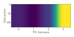
(a) Original (true, uncompressed).

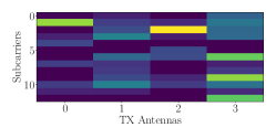
(b) Compressed $\kappa=0.9$.

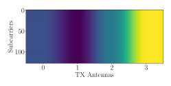
(c) Reconstructed $\kappa=0.9$.

Figure 3: The CDL-E channel state information matrix $\mathbf{H}$ for the first receive antenna and a given user under different scenarios: uncompressed, compressed, and reconstructed at a given transmit SNR $\rho$.

IV Performance Measures

Bit error rate: We define the empirical bit error rate (BER) as the ratio of bits that were received incorrectly (compared to the transmitted ones) as a result of the channel compression, fading, and noise. Let a given codeword of the $n$-th transmission be designated by a string of bits $\mathbf{x}^{(n)}\coloneqq(x^{(n)}_{1},x^{(n)}_{2},\ldots,x^{(n)}_{W})$. Therefore for $N_{\text{trans}}$ number of transmissions for a given UE:

$$p_{b}\coloneqq\frac{1}{N_{\text{trans}}W}\sum_{n=1}^{N_{\text{trans}}}\sum_{i=1}^{W}\mathbbm{1}[x^{(n)}_{i}\neq\hat{x}^{(n)}_{i}]$$ (5)

Block error rate: Further we compute the block error rate (BLER) defined as the probability of the CRC mismatch between the transmitted and received codeword based on the number of transmissions:

BLER $$\coloneqq\mathbb{P}[\mathbf{c}(\mathbf{x})\neq\mathbf{c}(\mathbf{\hat{x}})]$$ (6)

$$=\frac{1}{N_{\text{trans}}}\sum_{n=1}^{N_{\text{trans}}}\mathbbm{1}[\mathbf{c}(\mathbf{x}^{(n)})\neq\mathbf{c}(\mathbf{\hat{x}}^{(n)})]$$

The CRC is calculated based on a generator polynomial $\mathbf{c}(\cdot)$ with a finite length. It is appended to the end of every transmitted codeword regardless of the number of streams, with zero-padding as necessary to ensure that the codewords divide $N_{\text{sc}}N_{s}$ (without a remainder).

TABLE I: System Parameters

Parameter	Value
Channel model	CDL-C and CDL-E [10]
Modulation	$16$-QAM
Number of transmit antennas $N_{t}$	$4$
Number of receive antennas $N_{r}$	$4$
Number of OFDM subcarriers $N_{\text{sc}}$	$128$
Number of pilot symbols $N_{\text{pilot}}$	$10$
CRC length	$8$ bits
Number of users $N_{\text{UE}}$	$10$
Center frequency	$2100$ MHz
Subcarrier spacing $\Delta f$	$15$ kHz

TABLE II: Autoencoder Hyperparameters

Layer	Parameter	Value
Encoder	Depth	$2$
	Width	$(10,10)$
	Activation	(ReLU, ReLU)
Latent layer	Width	$2N_{r}N_{t}\lceil(1-\kappa)N_{\text{sc}}\rceil$
Decoder	Depth	$2$
	Width	$(10,N_{r}N_{t}N_{\text{sc}})$
	Activation	(ReLU, sigmoid)

(a) Bit error rates

(b) Block error rates

Figure 4: Bit and block error rates as a function of the transmit SNR $\rho$ for several values of $\kappa$ compared to the case of no compression (i.e., the baseline).

V Simulation

V-A Setup

We simulate the system outlined in Section II with the parameters in Table I. Users are represented as different random seeds in the simulation [12]. The equalizer $\mathbf{W}$ is the minimum mean squared error. We construct an autoencoder with the hyperparameters shown in Table II in addition to an epoch count of 128 and a batch size of 32. Further we simulate several compression ratios $\kappa\in\mathcal{K}\coloneqq\{0.4,0.7,0.9\}$. We use BLER generator $\mathbf{c}(\mathbf{x})=x^{6}+x^{4}+x+1$. We assume full-buffer transmission and choose a $60$-kilobyte bitmap image as the transmitted payload. The quantizer function $Q(\cdot)$ is set to truncate past the sixth decimal. We simulate for a set of transmit SNRs, $\rho\in\{0,5,\ldots,30\}$ for performance insights.

(a) Normalized run time

(b) Training and validation losses

Figure 5: Autoencoder normalized run time vs. $\kappa$ (left) and losses vs. the number of epochs for $\kappa=0.4$ (right).

TABLE III: Optimal transmit SNR for a given $\kappa$ at $B_{\text{max}}=0.1$

	CDL-C $\rho^{\star}$	CDL-E $\rho^{\star}$
Baseline	$20.53$ dB	$12.79$ dB
$\kappa=0.4$	$20.08$ dB	$13.19$ dB
$\kappa=0.7$	$20.08$ dB	$13.19$ dB
$\kappa=0.9$	$19.51$ dB	$13.24$ dB

V-B Discussion

We start with Fig. 3 which visualizes three variants of the CSI at the first receive antenna and $\kappa=0.9$: original uncompressed, compressed, and reconstructed (or decompressed). The size of data representing the subcarriers has reduced to a size equal to the latent layer dimension $\lceil(1-\kappa)N_{\text{sc}}\rceil=13$ from $N_{\text{sc}}=128$.

While the reconstructed channel does not perfectly resemble the original one—since autoencoder compression is lossy—the high degree of correlation in the CDL-E channel due to LOS propagation, provides the compression adequate redundant information for a useful reconstruction. However, in the CDL-C channel NLOS propagation, the limited degree of correlation (i.e., rich scattering environment) makes reconstruction more challenging. Thus, we conclude that 1) there is a limit to the size of the data representing subcarriers that can be eliminated due to the compression and 2) compression has better LOS propagation performance than NLOS propagation.

A question now arises: How far better can this compression be? In other words, what BER and BLER performance can be obtained for a given the compression ratio $\kappa$ and the transmit SNR $\rho$? To answer this question we study Fig. 4. Here, we observe that the performance of the system (as measured by the BER and BLER) degrades as $\kappa$ increases, which is an expected behavior due to the inability to perfectly equalize the channel after the lossy compression. Thus to find optimal transmission conditions (i.e., the minimum suitable $\rho$) for a given $\kappa$, we write

$$\rho^{\star}\coloneqq\max_{\rho\in\mathcal{S}} B\coloneqq\text{BLER}(\mathbf{x},\mathbf{\hat{x}};\rho,\kappa)$$ (7)

s.t. $$B\leq B_{\text{max}},$$

$$k\in\mathcal{K},$$

which is intractable due to the absence of a closed form of BLER (6) as a function of the compression rate $\kappa$ and SNR $\rho$. Thus, we resort to a search in $\kappa$ in a discrete subset of values at a set of discrete values of $\rho$. Table III shows an output of such a search in the two-dimensional space $\mathcal{S}\times\mathcal{K}$ at a target BLER $B_{\text{max}}=0.1$ per industry standards [13]. For this purpose, we define $\mathcal{S}\coloneqq\{\rho\mid 0\leq\rho\leq 30\}$ and find the minimum necessary SNR not exceeding $B_{\text{max}}$ for both NLOS and LOS propagation. The outcome is that compression is suitable for the high SNR regime of a given modulation. However, there is a performance gap in the SNR due to LOS vs. NLOS propoagation (in our case this gap is $6$-$8$ dB). This can be explained due to the increase in independent scattering in NLOS making redundant (or correlated) elements of information more scarce for the compression exploitation.

Finally, Fig. 5 shows the normalized run time of the autoencoder to be constant irrelative to the compression ratio and the training and validation losses of the deep autoencoder as a function of the number of training epochs for both channels. Given that both decrease monotonically, we conclude that the autoencoder is not overfitting and thus its results can be generalized within the values assumed by the CSI.

VI Conclusion

In this paper, we demonstrated the usefulness of autoencoders—as an element of a neural receiver in 6G—to compress the channel state information exploiting redundant information due to correlation. We showed that compression is useful in high SNR regimes, which correspond to a dominant line of sight or users at the cell center. This procedure is a step closer towards an AI-enabled air interface in 6G.

References

- [1] F. B. Mismar, A. AlAmmouri, A. Alkhateeb, J. G. Andrews, and B. L. Evans, “Deep Learning Predictive Band Switching in Wireless Networks,” IEEE Trans. on Wirel. Commun., pp. 96–109, Jan. 2021.
- [2] 3GPP, “Study on Artificial Intelligence (AI)/Machine Learning (ML) for NR air interface,” 3rd Generation Partnership Project, TR 38.843, Jan. 2024, v18.0.0.
- [3] F. B. Mismar, A. Gündoğan, A. O. Kaya, and O. Chistyakov, “Deep Learning for Multi-User Proactive Beam Handoff: A 6G Application,” IEEE Access, vol. 11, pp. 46 271–46 282, 2023.
- [4] F. B. Mismar, B. L. Evans, and A. Alkhateeb, “Deep Reinforcement Learning for 5G Networks: Joint Beamforming, Power Control, and Interference Coordination,” IEEE Transactions on Communications, vol. 68, no. 3, pp. 1581–1592, 2020.
- [5] Y. Zhang, X. Zhang, and Y. Liu, “Deep Learning Based CSI Compression and Quantization With High Compression Ratios in FDD Massive MIMO Systems,” IEEE Wireless Communications Letters, vol. 10, no. 10, pp. 2101–2105, 2021.
- [6] J. Guo, C.-K. Wen, S. Jin, and G. Y. Li, “Overview of Deep Learning-Based CSI Feedback in Massive MIMO Systems,” IEEE Transactions on Communications, vol. 70, no. 12, pp. 8017–8045, 2022.
- [7] M. K. Shehzad, L. Rose, S. Wesemann, and M. Assaad, “ML-Based Massive MIMO Channel Prediction: Does It Work on Real-World Data?” IEEE Wirel. Commun. Lett., vol. 11, no. 4, pp. 811–815, 2022.
- [8] H. Liu and K. Long, “A Deep Learning Channel Estimator for Millimeter-Wave Hybrid Massive MIMO Systems,” IEEE Wireless Communications Letters, vol. 12, no. 12, pp. 2103–2107, 2023.
- [9] H. Son and Y.-H. Cho, “Analysis of Compressed CSI Feedback in MISO Systems,” IEEE Wirel. Commun. Lett., vol. 8, no. 6, Aug. 2019.
- [10] 3GPP, “5G; Study on channel model for frequency spectrum above 6 GHz,” 3rd Generation Partnership Project, TR 38.900, Jun. 2018.
- [11] D. P. Kingma and J. Ba, “Adam: A Method for Stochastic Optimization,” in Proc. International Conf. on Learning Representations, May 2014.
- [12] F. B. Mismar, “A Quick Primer on Machine Learning in Wireless Communications,” Dec. 2023.
- [13] 3GPP, “5G; NR; Requirements for support of radio resource management,” 3rd Generation Partnership Project, TS 38.133, Oct. 2018.