MagMar III - Resisting the Pressure, Is the Magnetic Field Overwhelmed in NGC6334I?
Abstract
We report on ALMA observations of polarized dust emission at 1.2 mm from NGC6334I, a source known for its significant flux outbursts. Between five months, our data show no substantial change in total intensity and a modest 8% variation in linear polarization, suggesting a phase of stability or the conclusion of the outburst. The magnetic field, inferred from this polarized emission, displays a predominantly radial pattern from North-West to South-East with intricate disturbances across major cores, hinting at spiral structures. Energy analysis of CS emission yields an outflow energy of approximately ergs, aligning with previous interferometric studies. Utilizing the Davis-Chandrasekhar-Fermi method, we determined magnetic field strengths ranging from 1 to 11 mG, averaging at 1.9 mG. This average increases to 4 mG when incorporating Zeeman measurements. Comparative analyses using gravitational, thermal, and kinetic energy maps reveal that magnetic energy is significantly weaker, possibly explaining the observed field morphology. We also find that the energy in the outflows and the expanding cometary H II region is also larger than the magnetic energy, suggesing that protostellar feedback maybe the dominant driver behind the injection of turbulence in NGC6334I at the scales sampled by our data. The gas in NGC6334I predominantly exhibits supersonic and trans-Alfvenic conditions, transitioning towards a super-Alfvenic regime, underscoring a diminished influence of the magnetic field with increasing gas density. These observations are in agreement with prior polarization studies at 220 GHz, enriching our understanding of the dynamic processes in high-mass star-forming regions.
1 INTRODUCTION
Stars are formed within dense and weakly ionized gas and dust complexes commonly known as molecular clouds, where the current paradigm suggests that they are filamentary in nature (Arzoumanian et al., 2011). Despite their weakly ionization rates, magnetic fields thread these regions and are unavoidable. In the past decades, the advent of millimeter and submillimeter interferometers such as Berkeley, Illinois and Maryland Association (BIMA), the Combined Array for Research in Millimeter-wave Astronomy (CARMA), and Sub-Millimeter Array (SMA) began to allow surveys of magnetic fields in a sample of star forming regions (Rao et al., 1998; Cortes et al., 2005; Hull et al., 2014; Zhang et al., 2014b). The arrival of the Atacama Large millimeter/sub-millimeter Array (ALMA) and the James Clerk-Maxwell Telescope JMCT-Pol2, further improve the understanding of the effects of magnetic fields in star forming regions (Pattle et al., 2023). However, a complete understanding of their effects is still elusive. This is particularly evident when studying the formation of high-mass stars (over 8 M⊙) because of their relative faraway distances and the complexity inherent to the high-mass star formation process. Through the detection of polarized emission from dust, where the main assumption is that dust-grains are align by magnetic fields, detailed projected magnetic field morphology maps have been uncovered by ALMA from number of high-mass star forming regions (e.g. Cortes et al., 2016; Beltrán et al., 2019; Liu et al., 2020; Sanhueza et al., 2021; Fernández-López et al., 2021; Cortes et al., 2021a; Cortés et al., 2021b; Beuther et al., 2023; Liu et al., 2023a, b). Here, we delve into the magnetic environment surrounding one of these high-mass star-forming clumps, NGC6334I, as part of the Magnetic fields in Massive star-forming Regions (MagMar) collaboration (Sanhueza, 2024). NGC6334I is a part of the vast Giant Molecular Cloud (GMC) NGC6334, situated within the Sagittarius-Carina spiral arm, approximately kpc away from the Sun (Chibueze et al., 2014). Despite NGC6334 vastness ( pc), the regions of NGC6334I and NGC6334I(N) concentrate most of the studies in the millimeter and sub-millimeter range of the spectrum (McCutcheon et al., 2000; Hunter et al., 2014, 2017; Sadaghiani et al., 2020). A notable characteristic of NGC6334I is a significant millimeter flux outburst, predominantly centered on the MM1B proto-stellar core (Brogan et al., 2016; Hunter et al., 2017, 2018; Brogan et al., 2018). This flux surge was accompanied by a flare in multiple maser species, particularly the OH maser transition which offered insights into line-of-sight (LoS) magnetic field strengths (MacLeod et al., 2018). Moreover, several methanol maser lines, some previously unobserved, flared around the MM1 proto-cluster, hinting at a possible accretion event. Furthermore, outflow emission is also observed throughout NGC6334I. Initially detected in CO by Bachiller & Cernicharo (1990) using the IRAM 30 meter telescope, outflow emission was later observed in CS by McCutcheon et al. (2000) using the JCMT, and by Beuther et al. (2008) in HCN using the Australian Compact Array (ATCA). Later, ALMA observations of CS spatially resolved the emission finding four bipolar outflows where the most prominent one appears to originate from the MM1 proto-cluster (Brogan et al., 2018). Finally, the magnetic field in NGC6334I has been mapped by the SMA (Zhang et al., 2014a, c; Li et al., 2015), the JCMT POL2 instrument at resolution (Arzoumanian et al., 2021) and by ALMA at 1.4 mm (220 GHz) and 0 resolution (Liu et al., 2023b). Here, we present 1.2 mm (250 GHz) and 0 resolution mapping of the magnetic field in NGC6334I. The ensuing sections are structured as follows: Section 2 outlines the observation techniques, calibration, and data analysis methods; Section 3 unveils the results from the polarized dust emission; Section 4 presents the discussion. We encapsulate our findings and conclusions in Section 5.
2 OBSERVATIONS
NGC6334I was observed as part of project 2018.1.00105.S, which was executed twice in session mode (see chapter 8 in Cortes et al., 2023, for details about the session observing mode), on December 13th 2018 and on May 4th 2019 under configuration C43-4 (providing baseline lengths from 15 to 783 m). The correlator was configured to yield full polarization cross correlations ( and ) using the Frequency Division Mode (FDM), including spectral windows to map the dust continuum and windows centered on a number of molecular line rotational transitions relevant to the study of high-mass star formation (see Table 1), with an effective wavelength of 1.2 mm. The bandpass was calibrated using J1427-4206 for session 1 and J1924-2914 for session 2. The time dependant gain and the instrumental polarization terms were calibrated using J1717-3342 and J1751+0939, respectively. For calibration we used CASA version 5.4 and version 5.6 for imaging (CASA Team et al., 2022). To image the continuum, we manually extracted the line-free channels from each spectral window, which we later phase-only self-calibrated using a final solution interval of 90 seconds. These solutions were then applied to all of the molecular line transitions presented here before imaging. The spectral cubes were produced by using 2 km s-1 channel width. The statistics of the flat Stokes images, before debiasing, for both continuum and channel maps are shown in Table 2. All of the Stokes parameters were imaged independently using the CASA task tclean, which yielded an angular resolution of approximately , with a position angle of -78∘. The data were primary beam corrected and debiased pixel-by-pixel following Wardle & Kronberg (1974) and Hull & Plambeck (2015). Finally, we also obtained archival data from project 2017.1.00793.S which also observed NGC6334I, but using a lower frequency spectral setup with an effective wavelength of 1.3 mm (see Liu et al., 2023, and Table 1). These data were also obtained in two sessions on June 28th 2018 and September 2nd 2018, roughly two months apart. We did not combined these datasets, but briefly compared the polarized dust emission (see section 3 and appendix A).
| Band | Spw 1 | Spw 2 | Spw 3 | Spw 4 | Spw 5 | Spw 6 | Spw 7 | PA | |||||||||
|---|---|---|---|---|---|---|---|---|---|---|---|---|---|---|---|---|---|
| (GHz) | (kHz) | (GHz) | (kHz) | (GHz) | (kHz) | (GHz) | (kHz) | (GHz) | (kHz) | (GHz) | (kHz) | (GHz) | (kHz) | (′′) | (′′) | (°) | |
| 6 | 261.245 | 244 | 260.277 | 244.141 | 257.523 | 976 | 245.520 | 976 | 243.520 | 976 | - | - | - | - | 0.45 | 0.4 | -82.8 |
| 6 | 216.430 | 976 | 218.54 | 976 | 233.54 | 976 | 230.528 | 122 | 231.051 | 122 | 231.211 | 122 | 231.312 | 122 | 1.7 | 1.1 | 87 |
| 6 | 216.430 | 976 | 218.54 | 976 | 233.54 | 976 | 230.528 | 122 | 231.051 | 122 | 231.211 | 122 | 231.312 | 122 | 0.7 | 0.5 | 68 |
Note. — The spectral configuration and beam sizes from the MagMaR project (row 1) are detailed here along with the configuration used by project 2017.1.00793.S (rows 2 amd 3). For each spectral window (e.g. Spw 1), the center frequency is indicated in GHz, along with the channel width in kHz (e.g. ). The synthesized beam parameters (angular resolution) for both projects are the major axis , minor axis , and position angle PA. Note, project 2017.1.00793.S was observed in two different configurations hence the two different beam sizes between row 2 and 3.
| Stokes | Max | Mean | |
|---|---|---|---|
| () | () | () | |
| I | 1300 | 33.0 | 998 |
| Q | 4.1 | -0.01 | 55 |
| U | 4.1 | 0.07 | 55 |
| V | 1.6 | 0.03 | 76 |
Note. — The Stokes Images statistics, from the combined sessions, are listed here. Note, Stokes is dynamic range limited; also, Stokes , , and can be negative and thus, the maximum is not necessary a positive value. Furthermore, note that the units of Stokes , , and are are . The Stokes values from ALMA observations are subject to larger uncertainties than linear polarization (see Cortes et al., 2023).
3 RESULTS
3.1 The Dust Continuum Emission
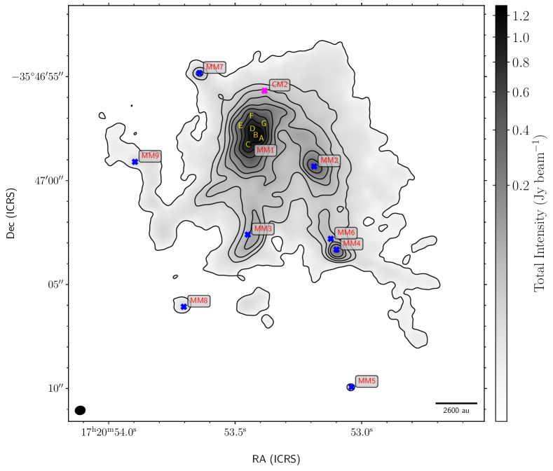
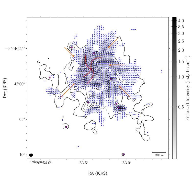
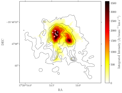
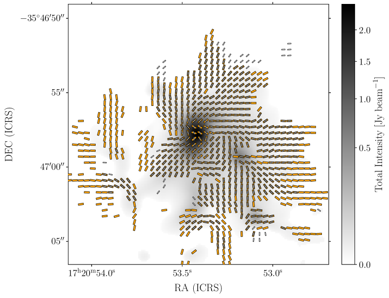
Figure 1 shows the NGC6334I total intensity (Stokes I) map from the ALMA 1.2 mm continuum data. The most massive sources previously identified by Brogan et al. (2016) are detected and are indicated by blue crosses in the map. The dust continuum map at 250 GHz is also consistent with the lower frequency data obtained by Liu et al. (2023b) (see appendix A). The massive proto-cluster MM1 is not resolved in our data; nonetheless, we have superposed the individual peaks identified by Brogan et al. (2016) following their nomenclature and position. The unusual source CM2, a strong water maser source with an ambiguous origin and also detected in radio continuum, is also seen in our data at the level in dust emission, where mJy beam-1 (see Table 2 and Tables in Brogan et al., 2016). The UC H II region from the MM3 core is well constrained which give us confidence that most of the emission at 250 GHz is coming from dust grains.
Since our data were acquired by executing two sessions separated by roughly five months, we explored the flux variability reported by Hunter et al. (2021), and references therein. To this effect, we imaged each session independently in all Stokes. We found that the differences between the flux in the MM1 proto-cluster was below 1%, below the ALMA accuracy of band 6 ( 10%). Because the 2017.1.00793 data (220 GHz) were taken on different configurations and only 2 months apart, comparing the two is difficult therefore we omit it here on. We also explored variability in the polarized flux where we found variability in Stokes and in the order of 8% (see Table 3). Note, the minimum amount of detectable linear polarization by ALMA is estimated to be 0.1%, as established from point source measurements (Cortes et al., 2023). Because the flux variability in Stokes during this period was negligible, this suggests that the outburst might have already finished or the emission is below our sensitivity. Although a variability of 8% in and within six months appears intriguing, its analysis is out of the scope of this work and we defer it to a future investigation.
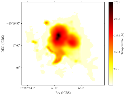
3.2 Column Density and Mass
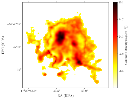
Calculating the column density from dust emission at millimeter wavelength is a well established procedure. Here, we use the standard formulation developed by Hildebrand (1983) but we make use of the NGC6334I temperature model obtained by Liu et al. (2023b) from Methanol emission where we assume that the gas emission is optically thin and that the gas and dust are in thermal equilibrium (see Figure 2). The temperature model map was extended to match the dust emission spatial distribution detected by ALMA to the level. To extend the model temperature map, we assumed that the dust temperature converged to 30 K outside the original model map. This is justified given the results from McCutcheon et al. (2000); Sandell (2000) who derived a dust temperature value of 30 K for NGC6334I using all available millimeter and millimeter data at the time. The map was later smoothed using a Savitzky-Golay smoothing filter (Savitzky & Golay, 1964) with a window of one beam to ensure continuity111The Savitzky-Golay filter is a digital filter that can be applied to a set of digital data points for the purpose of smoothing the data. This is achieved by fitting successive subsets of adjacent data points with a low-degree polynomial by the method of linear least squares. We use this filter to smooth the temperature map because the filter is particularly useful to preserve important features of the data, such as relative maxima, minima, and width, which are often ”washed out” by other types of smoothing filters.. Besides the temperature model, we used a dust emissivity cm2 gr-1 for the dust grains at 230 GHz (Ossenkopf & Henning, 1994), and a gas to dust ratio of a 100 and the assumption that the dust emission is optically thin. The column density map in log scale is shown at Figure 2. Note, because the temperature model derived by Liu et al. (2023b) may have used optically thick CH3OH emission, we may be overestimating the temperature in the most dense regions of the clump, which would lead to under-estimations of the column density. Nonetheless, the column density values at the core positions in our map appear to be in agreement with Brogan et al. (2016) who observed NGC6334I with ALMA and the VLA computing Spectral Energy Distributions (SED) for the major sources in the region deriving temperatures and densities. By having a column density map222Note, we are deriving here a magnetic field map which has values per pixel. However, the limiting resolution factor is given by the synthesized beam of the telescope which should be taken into account when deriving conclusions from these maps. , we can estimate a map of the mass. We do this by computing , where are map pixel indexes along right ascension and declination respectively, is the area of each pixel, is the mass of Hydrogen, is the mean molecular weight, and is the column density per pixel.
3.2.1 The Number Density Map
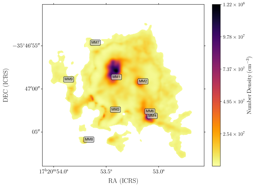
Because of the complicated morphological features seen in the dust emission, it is difficult to model the spatial distribution of the dust and determine its volume density. A simple approach is to assume that the whole region is a cylinder of a certain thickness which can be estimated from the dust emission intensity profile. Opting for a cylindrical rather than spherical geometry could be more appropriate for several reasons. While a spherical model encompassing all dust emission at the 3 level indicates a mean radius of approximately 0.02 pc, leading to average and peak number densities significantly lower than those observed in ALMA studies of the region, a cylindrical model offers more flexibility. By adjusting the cylinder’s height, it becomes possible to align the modeled core densities more closely with the observed densities ranging between cm-3, as reported by Brogan et al. (2016); Sadaghiani et al. (2020). This approach allows for a more accurate representation of the physical conditions within these dense cores. Note, this simple geometrical assumption assumes the same height throughout NGC6334I which is not accurate. It is more likely that the cores in this region will follow a power law density profile different from the rest of the surrounding gas. Thus, we choose the height of the cylinder looking for a drop in the intensity as a function of distance from the peak emission and assume that this length corresponds to the height. The number density per pixel is determined then by computing , where is the thickness of the cylinder. By doing this, we find a drop in the intensity at the level in the dust emission which corresponds to or 0.03 pc at a distance of 1300 pc. The values presented in our number density map align with those established by Brogan et al. (2016), which were derived from Spectral Energy Density (SED) fitting to ascertain dust temperatures and under the assumption of spherical geometry.
3.3 The Magnetic Field Morphology from Polarized Dust Emission
Figure 3 displays the magnetic field morphology on the plane of the sky, derived from polarized dust emission under the assumption of grain alignment by magnetic fields (Lazarian & Hoang, 2007), which assumes a 90∘ rotation in the linear polarization position angle. While alternative alignment mechanisms such as radiative alignment (Tazaki et al., 2017) and self-scattering (Kataoka et al., 2016) have been proposed, the scales and physical conditions in massive star-forming regions (like the radiation anisotropy and large grain sizes), make them less favored. Consequently, magnetic alignment emerges as the most probable process driving the polarized emission detected towards NGC6334I. The polarized emission encompasses most of the primary sources in NGC6334I, including MM1, MM2, MM4, MM6, MM7, MM9, and CM2 (a strong water maser source with an ambiguous origin). Notably, the cometary UCH II region MM3 lacks significant polarized dust emission, thus leaving its magnetic field untraced (refer to Figure 1 in Sadaghiani et al., 2020, for the extent of the MM3 UCH II). The field morphology, albeit intricate, reveals consistent patterns across certain directions. For instance, the field demonstrates an evolution from North-West to South-East, showing discernible changes over the fragmented MM1 core, possibly a radial morphology towards the MM1 center of mass (see Figure 4). Similarly, indications of radial configurations in the field lines can also be seen around the MM2 and MM4/MM6 cores. Radial morphologies suggests that gravity dominates and drags the field towards the center of mass (Tang et al., 2009; Girart et al., 2013; Koch et al., 2018; Cortes et al., 2016, 2019; Koch et al., 2022). Noteworthy discontinuities, such as roughly shifts in field direction between adjacent pseudo-vectors, appear at the fringes of MM1 over the MM2 core and between MM6 and MM1. Despite these discrepancies, the field predominantly appears coherent on scales of – (equivalent to 6500 to 13000 au, as visualized in Figures 1 and 3). Spiral field patterns, like those observed in G327 and IRAS 18089 (Beuther et al., 2020; Sanhueza et al., 2021), where spiral attributes are conspicuous and where rotation and infall have been deemed dynamically significant, maybe present at the inner regions of the MM1 proto-cluster (see Figure 4). However, clear rotation signatures are not conclusive from our data. Nonetheless, small scale spiral patterns have been observed in other high mass sources. Burns et al. (2023) observed spiral signatures on the also out-bursting source G358.93-0.03-MM1 from high spatial resolution (50 to 900 au), 6.7 GHz methanol maser emission. Based on these results, it is plausible that, in NGC6334I, the indications of spiral morphologies seen in the field are retain in the gas, but not resolved due to the limitations of the ALMA configuration used here.
3.4 Molecular Line Emission
The spectral setup used by the MagMar project allow the detection of molecular line emission from a number of tracers usually abundant in high mass star forming regions. From our data, we used CS and C33S to study outflow and non-thermal motions. From the data obtained by Liu et al. (2023b), we extracted the 12CO emission which we used to study the outflows present in NGC6334I.
| Stokes | Maxs1 | Means1 | Maxs2 | Means2 | variability | ||
|---|---|---|---|---|---|---|---|
| () | () | () | () | () | () | (%) | |
| I | 1330 | 45 | 0.988 | 1331 | 42 | 1.0 | 0.1 |
| Q | 3.91 | 0.028 | 0.067 | 4.3 | -0.007 | 0.073 | 8 |
| U | 3.97 | 0.075 | 0.083 | 4.3 | 0.088 | 0.068 | 8 |
| V | -1.06 | -0.003 | 0.083 | 2.8 | 0.06 | 0.100 | - |
Note. — The flux density variability for all Stokes continuum images is listed listed here. The values where extracted from the images considering the 1/3 FWHM for the maximum and the mean while we used a region devoid of emission for . The subscript s1 and s2 indicates session 1 and session 2. Note, Stokes , , and can be negative and thus, the maximum is not necessary a positive value. We do not list the variability in Stokes V due to the large ALMA uncertainties with circular polarization.
3.4.1 The Emission
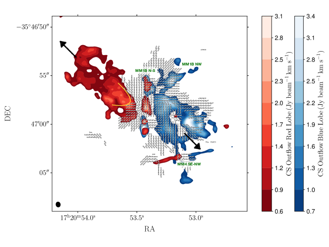
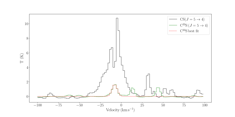
Figure 5 displays a moment zero map of the CS emission towards NGC6334I, where the data have been categorized into redshifted and blueshifted velocity components to show outflow emission. This categorization was done by considering a systemic velocity of -7.56 km s-1, as determined by a Gaussian fit to the C33S line (refer to section 3.4.2), with velocity intervals of -40 to -12 km s-1 for the blueshifted and -4 to 12 km s-1 for the redshifted components. Outflow emission is clearly seen in the CS moment zero map, where our data align with the morphological findings of Brogan et al. (2018). Following their nomenclature, our map reproduces the prominent NE-SW, the MM1B N-S, the MM1B NW, and the MM4 SE-NW outflow emissions as indicated in Figure 5. From the four outflows detected towards NGC6334I, the NE-SW outflow appears to be dominant. Although its exact origin has not been conclusively determined, it appears to emerge from the MM1 proto-cluster which is also the likely origin of the smaller MM1B N-S and MM1B NW outflows. From the map, the NE-SW outflow red-lobe appears to be carving a cavity in the dust as shown in Figure 5. The edges of this cavity seem to be traced by magnetic fields as we will show later (see section 4). To study the CS emission in more detailed, we modeled the data using the MADCUBA package which fits spectroscopy models to the data using a complete radiative transfer formalism under a Local Thermodynamic Equilibrium (LTE) assumptions (Martín et al., 2019). To this effect, we extracted a spectrum from the central region of NGC6334I containing the CS line and a number of other molecular transitions (see Table 1 for a description of the spectral windows containing the CS line). This spectrum was modeled with the MADCUBA package where we found that the CS line would be optically thick () assuming an excitation temperature K derived with available transitions of , , and in the observed spectral windows, and based on the C33S fit and assuming a 32S/33S=102 taken from (Yu et al., 2020), since the CS profile is heavily affected by self-absorption.
3.4.2 The ) Emission
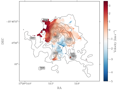
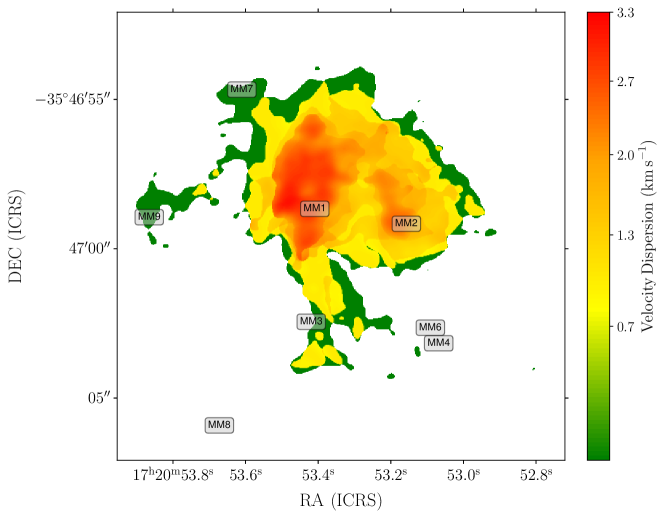
The C33S() emission appears to be compact and confined to the brightest dust emission contours, as shown in Figure 6. The peaks in the integrated intensity map coincide with the dust emission peaks while most of the C33S is confined within the contour from the dust emission. While the MM1 proto-cluster is not resolved in the dust emission, three distinct condensations are observable in C33S from North to South and around the dust peak, which are loosely associated with the condensations resolved by the higher resolution ALMA data (Brogan et al., 2016) as indicated by the white crosses in Figure 6. Toward MM2, the C33S peak emission aligns well with the dust maxima, whereas the emission levels appear marginal toward MM4 and MM7, and remain undetected toward MM9. In Figure 6, the moment 1 map is also presented, relative to V, obtained through Gaussian fitting of the C33S spectrum from the 1/3 FWHM of the primary beam. From this map, a velocity gradient is seen from North-East to South-West which is consistent with that obtained by Liu et al. (2023b) using the OCS molecular emission, though our coverage does not match the extent of the ALMA mosaic in Liu et al. (2023b). Although the velocity gradient might have some outflow contamination, the spectra shown in Figure 6 suggests it should be minimal. This is because the C33S line profile is almost completely Gaussian with very small deviations around the -20 km s-1 velocity channel. Thanks to the lack of absorption features, we could fit the C33S spectrum with the same temperature assumption done for CS above, which suggests that the emission is optically thin (tau=0.3) which allows to use the moment 2 map as the velocity dispersion along the line of sight (see Figure 7).
3.4.3 The ) Emission
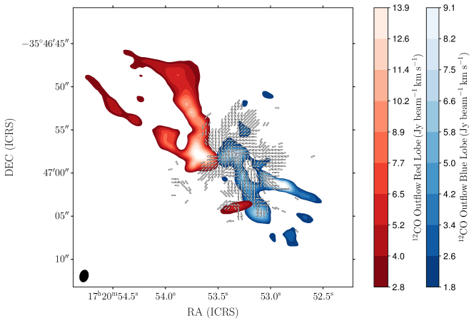
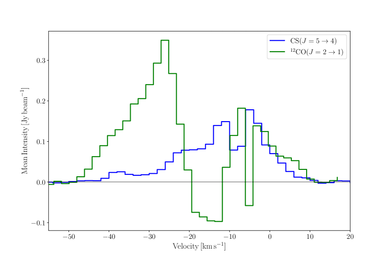
We used the ALMA data obtained by Liu et al. (2023b) to image the outflow emission from NGC6334I (see Table 1 for a description of their data). To image the outflow emission we used a velocity interval from -45 to -25 km s-1 for the blue lobe and -4 to 11 km s-1 for the red lobe (refer to Figure 5, which displays the combined data from both ALMA configurations). From these data, only the NE to SW outflow is clearly discernible, whereas the N-S outflow in the line of sight remains undetected in 12CO and some traces of the MM1B NW outflows are seen in the blue-lobe. Additionally, only the red-lobe of the MM4 outflow is observable in 12CO. As with the CS emission, the red-lobe of the CO outflow appears to be carving a cavity in the dust where the magnetic field traces the edges of the cavity (see section 4). Although this data set includes configuration C41, the most compact ALMA configuration with a Maximum Recoverable Scale (MRS) of (0.06 pc at 1300 pc, the distance to NGC6334I), there appears to be significant extended emission from 12CO that the interferometer is resolving out. Figure 8 shows CO and CS spectra superposed to each other. Although the outflow emission is seen in both molecular profile line-wings, the comparison suggests, as previously mentioned, that significant emission from CO is missing. This is likely either due to filtering effects or self-absorption (see section 3.4.3). Therefore, we omit using CO emission for the outflow analysis here.
4 DISCUSSION
At first glance, the magnetic field in NGC6334I displays a complex morphology which is difficult to associate with a projection from a simple shape, such as the “hourglass” proposed by models (Ciolek & Mouschovias, 1994) and observed in numerous star-forming regions (Girart et al., 2006; Hull et al., 2014; Li et al., 2015; Beltrán et al., 2019; Cortés et al., 2021b). Although there are indications of a radial pattern at the outskirts of the clump and in the direction of the MM1 proto-cluster, there are also hints of some sort of spiral arms in the field close to the central region of the MM1 proto-cluster (see Figure 4). The radial pattern can be explained by a dominant gravitational pull, but for the spirals, we do not find conclusive evidence of rotation or velocity gradients that can explain these features in the field morphology at these scales (see Figure 6). Nonetheless, small scale spiral patterns cannot be ruled out given previous finding in other similar high mass out-bursting sources (see Burns et al., 2023). Additional complexity in the field morphology arises from sudden 90∘ shifts in the field lines. These turns in the field morphology can be seen around the MM2, MM6 cores, and also at the interface of the MM1 proto-cluster as indicated by the red ellipses in Figure 3. These sharp shifts in the field morphology are challenging to elucidate; they could result from projection effects or perturbations in the field by the gas due to turbulence or gravity. One possibility is that the four outflows detected in this region might be perturbing the magnetic field structure. For instance, the most prominent bipolar outflow, seen in both CO and CS emission red lobe, appears to carve a cavity in the dust where the magnetic field seems to follow the edges of the cavity as indicated in Figure 5. Similar situations have been seen in low mass star forming regions such Serpens SMM1-b where the outflow emission was also found to trace the edges at the base of the outflow cavity (Hull et al., 2017). We also note that the field show some degree of alignment with the MM1B NW and the MM4 SE-NW outflows. However, whether this is a projection effect or real alignment cannot be concluded from these data. As understanding projection effects demands extensive numerical modeling, we instead examine whether the energy balance in NGC6334I could explain the perturbations seen in the field.
4.1 The Energy in the Outflows
To explore the quantitative effect of the outflow in the magnetic field, we attempt here to compute the outflow parameters in order to estimate their total energy. To derive the energy in the outflows, we used the CS emission rather than the CO emission. This is because the CO emission shows, what appears to be, significant filtering by the interferometer and possibly extensive self-absorption which will introduce larger errors in the estimations. Also, the CS line appears to better trace the outflows at the core scales mostly resolving all four outflows while the CO does not clearly show all of the outflow emission detected in NGC6334I (see Figure 5). However, it should be noted that because the interferometer does not recover all of the CS emission and because of the uncertainties in the abundance ratio between CS and H2, the outflow parameters derived here may have a large uncertainty. To estimate the outflow parameters, we extracted spectra from the CS velocity cube covering the extent of the CS moment 0 map (see Figure 7). Determining the outflow parameters require separating the emission coming from the gas at the source systemic velocity and the actual emission from the outflow. It also requires estimating the optical depth in the line-wings which is usually done by computing the line ratio with an isotopologue that has sufficient overlap in the line-wings covering the outflow emission. Unfortunately, the C33S emission detected towards NGC6334I is compact enough that the overlap with the CS at velocities associated with the outflow is minimal (see Figure 7). Thus, to estimate the CS column density corresponding to the outflow emission, we assume that this emission is optically thin in the channels covering the CS line-wings. The line-wings of the CS line cover the interval from -40 to -12 km s-1 for the blue lobe and -2 to 20 km s-1 for the red lobe where the systemic velocity of the source is determined to be -7.6 km s-1 as obtained from the Gaussian fit to the C33S line (see Figure 7). This interval covers all of the emission in the line-wings over 3, with K estimated from 25 line free channels. Note, we are not aiming to characterize independently the four outflows in this region, but rather estimate their bulk energy and its effect on the magnetic field.
By assuming that the emission is optically thin, we estimate the CS column density per velocity channel as (see Equation 16, Zhang et al., 2016),
| (1) |
where is the Boltzmann constant, is the Planck constant, is the speed of light in the vacuum, GHz is the rest frequency of the CS rotational transition, s-1 is the Einstein spontaneous emission coefficient, is the statistical weight, K is the energy level for the upper state, is the partition function, which for linear molecules is well approximated by , where GHz is the rotational constant for the CS molecule (Bustreel et al., 1979), is the channel width, and is the beam filling factor assumed to be 1. As indicated in Section 3.4.1, the excitation temperature, T K, is estimated from the modeling done with MADCUBA on symmetric rotor molecules. The mass of the outflow is calculated for every velocity channel as:
| (2) |
where corresponds to the mean molecular weight (Feddersen et al., 2020), is the Hydrogen mass, and is the area subtended by the region identified with the outflows (same used to extract the spectra from Figure 7), and is the total column density of the molecular Hydrogen where is the relative abundance of CS respect to the H2 in NGC6334I as determined from Herschel mapping (Zernickel et al., 2012). The momentum and kinetic energy per velocity channel is estimated as and where indicates the velocity channel used for each quantity (in this case is the mass spectrum, see Feddersen et al., 2020). The total mass, momentum, and energy is obtained by adding all velocity channels per lobe. The values for the mass energy and momentum are listed in Table 4. The assumption that the CS emission is optically thin the line-wings appears to be good enough to produce under-estimates of the total energy in the outflow when compared to single dish results. McCutcheon et al. (2000) estimated the kinetic energy on each outflow lobe to be ergs from their CO and CS millimeter single dish mapping while our estimates are an order of magnitude lower (see Table 4). Although, the mass, momentum, and energy are consistent with outflow properties from surveys of high mass protostellar outflows (Zhang et al., 2001, 2005), it should be noted that we are missing emission that might be present at the systemic velocity as well as the emission filtered out by the interferometer. Thus, the values derived here appear to be a lower bound for the outflow mass, momentum, and energy at these scales in NGC6334I.
| Source | Lobe | |||
|---|---|---|---|---|
| (M⊙) | (M⊙ km s-1 ) | ( ergs) | ||
| NGC6334I | Blue | 0.3 | 6.4 | 0.24 |
| NGC6334I | Red | 0.6 | 4.9 | 0.11 |
Note. — The Outflow parameters determined from the CS emission are presented here. The red lobe was obtained by considering a velocity range between -4 to 12 km s-1 while the blue lobe was obtained from a range between -40 to -12 km s-1.
4.2 The Magnetic Field Strength Map
To estimate the magnetic field strength on the plane of the sky, Bpos, we employed the Davis, Chandrasekhar, and Fermi technique (DCF, Davis, 1951; Chandrasekhar & Fermi, 1953) as outlined by Crutcher et al. (2004). In units of G, this can be expressed as:
| (3) |
where is the number density in cm-3, is the molecular linewidth from an optically thin species in km s-1 and is the dispersion in the magnetic field lines in degrees. Even though the DCF method has been revisited over time to explore its limitations and applicability (see reviews by Liu et al., 2021; Myers et al., 2024), we aimed to mitigate biases in this work by simplifying our analysis and minimizing assumptions. Consequently, we employed the “standard” DCF method, incorporating only the 1/2 correction proposed by numerical simulations (see Crutcher et al., 2004, for a comprehensive discussion). We will explore the implication of this in section 4.2.2.
Our objective here is to derive a map with estimations of the magnetic field strength onto the plane of the sky. To do that, we employ the number density model map, the velocity dispersion, , obtained from the C33S moment 2 map (see Figure 10), and a position angle dispersion map, . We use the C33S emission because is optically thin (see section 3.4.2), and thus it provides a good account of the non-thermal motions of the warm and dense gas. Although as we inspected the data cube only a single component of the line was observed, it is difficult to rule out, or remove, the small outflow contribution to the C33S emission. Nonetheless and because the emission is compact with very small deviation from the model at the linewings (see section 3.4.2), we assume that this contamination is minimal. Although it does not overlap completely with the polarized dust emission, the C33S emission has sufficient coverage around the most relevant cores in NGC6334I to provide a good account of turbulence in this region.
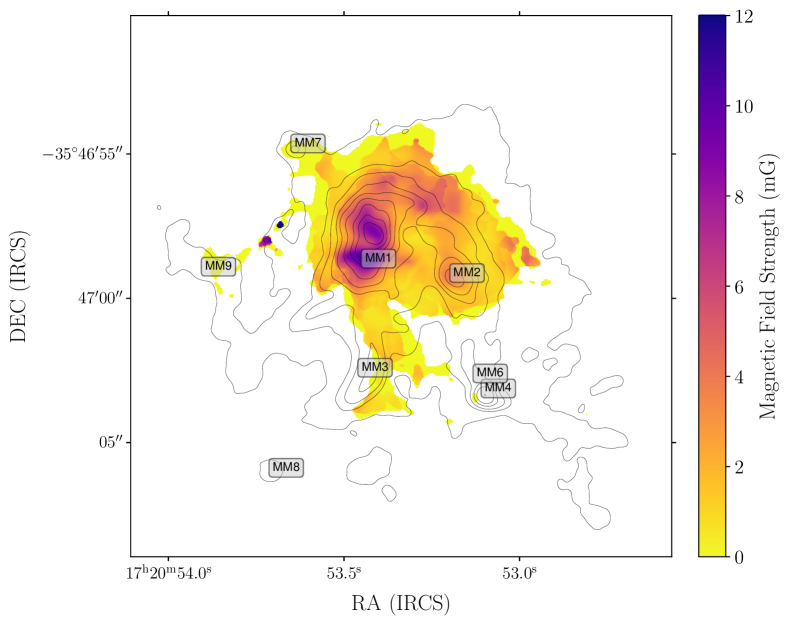
The dispersion in the magnetic field lines is obtained by taking the standard deviation over a moving window of in size. This kernel is the beam size, which give us about 16 independent points per window to calculate the standard deviation using circular statistics under the assumption of a 5∘ error in the polarization position angle (see Appendix B for a discussion about the statistics of the moving window). The window size used here has a sufficient statistical significance to produce a believable estimate for the angular dispersion, but also encloses the local fluctuations in the field, which are seen to occur in angular scales of by visual inspection. While our goal is to account for the best possible estimate of the magnetic field lines local dispersion, we also strive to prevent skewing our results in areas where the magnetic field appears uniform. To achieve this, we are cautious about selecting a larger moving window size, which could inadvertently include areas exhibiting significant fluctuations in the magnetic field’s direction (i.e. regions where the field shows turns). Therefore, a value of in size for the moving window appears to be a good compromise to achieve these objectives (Appendix B offers a more detailed discussion showing the effect of increasing the moving window size). Note, it is entirely plausible that the sudden turns in are due to projection effects and not because of perturbation in the field lines. If that were to be the case, the estimated dispersion from that regions would be artificially large, which will decrease the estimated field strength and thus the values around those regions should be considered as lower bounds for the magnetic field strength onto the plane of the sky. Thus and under these considerations, the Bpos map estimate is shown in Figure 9. The mean magnetic field strength estimated value is mG with a peak of 11 mG towards the MM1 proto-cluster. Note, a strong outlier to the East of MM1 appears to be the result of small statistics at that point which we ignore. Although Li et al. (2015) estimated B mG at scales of 0.1 pc from the SMA data, our mean value is lower which can be explained because of the coarser SMA resolution that smooths the field morphology and also because of their distance assumption to NGC6334 (1.7 kpc) which yields and overestimation of the mean density. Our estimate is consistent with the magnetic field strengths reported in a more recent analysis of the SMA data by Palau et al. (2021).
4.2.1 A total magnetic field estimation
Additional insight can be obtained from the results obtained by Hunter et al. (2018), who measured the magnetic field on the line of sight, Blos, by detecting the Zeeman effect from OH maser emission yielding magnetic field strengths between +0.5 and +3.7 mG towards the CM2 source and -2 to -5 mG around the MM3 H II region. Although their resolution, au, appears to be larger than the likely physical size of a maser spot, their measurements appears consistent with others (Caswell et al., 2011). We find our field estimates onto the plane of the sky, Bpos, consistent with this range in field strength. The OH maser emission detected by Hunter et al. (2018) is associated with regions within our map (CM2 and MM3) and with gas at densities in between cm-3 according to the models of Cragg et al. (2002), which are within the ranges covered by our density model. This allow us to estimate the total magnetic strength field by computing the vector sum . Hunter et al. (2018) found the distribution of OH masers to be well correlated with methanol masers at 6.7 GHz and with the MM3 UCH II region and CM2 source. However, there seems to be a consistent lack of maser emission towards the strongest continuum peaks in NGC6334I, particularly the MM1 proto-cluster where 80% of the maser emission is found outside the 40% level of the continuum in their ALMA 1 mm data. This suggests that the density in the strongest dust emission peaks in MM1 is too high to support inversion (Hunter et al., 2018). Thus, to add the OH Zeeman measurement to our magnetic field map, we decided to take the average of the absolute values from Hunter et al. (2018) Table 8, or mG, and compute the vector sum with the average of our values. This yield a total magnetic field estimate mG. In principle, one would have liked to add the Zeeman values following a density profile. However, the coverage of the maser emission is sparse and we lack of a well defined canonical shape of the field which might have allow us to produce a total magnetic field map. This estimate is consistent with extrapolations derived by assuming a field strength dependency with density of as obtained from CN Zeeman measurements (Crutcher & Kemball, 2019) and by estimations using the DCF method, and its variants, toward other HMSFR (Beltrán et al., 2019; Cortés et al., 2021b; Sanhueza et al., 2021).
4.2.2 Caveats
The DCF technique has a number of caveats which have been explored in a number of works (Heitsch et al., 2001; Crutcher et al., 2004; Falceta-Gonçalves et al., 2008; Cho & Yoo, 2016; Skalidis & Tassis, 2021; Cortes et al., 2019; Liu et al., 2021; Lazarian et al., 2022; Myers et al., 2024). Here, we mention the most important caveats that might be affecting the validity of our analysis in order to give perspective to the conclusions that we are deriving here. The DCF technique provides an estimate of the field strength onto the plane of the sky by assuming equipartition between turbulence and magnetic energy without considering self-gravitation and the anisotropic nature of turbulence. A region such as NGC6334I has already formed a number of protostars suggesting that the gas is far from an equilibrium situation. Although the effect of self-gravity in the dispersion of the position angle is difficult to quantify, gravity manifests itself over long distances requiring large reservoirs of mass to have a significant effect. Thus, the injection of turbulence by gravity into the gas, which will ultimately perturb the field, might happen at larger scales than the one traced by our moving box. Another issue relates to the velocity dispersion obtained from the C33S moment 2 map which contains contributions from the mean velocity field which in this region might come from the outflow, infalling motions, and (or) rotation, in addition to turbulence. These components cannot be immediately removed because we lack sufficient information about the kinematics and geometry of the source. In short, we might be overestimating the non-thermal motions due to turbulence which will bias the estimation of the field strength as well as the sonic Mach number (see section 4.4 for a discussion).
The estimation of the density model is also subjected to a number of assumptions which are almost impossible to quantify. For instance, the determination of the column density map in our data is not only affected by flux calibration and temperature model uncertainties, but also by line-of-sight contamination, field selection, and most importantly by interferometric spatial filtering (see Ossenkopf-Okada et al., 2016). Because we constructed the density model assuming a temperature model which may be overestimating the actual dust temperature, the values might be underestimations. In the case of the dispersion in the field lines, the proxy used here is the dispersion in the linear polarization angle of the ALMA polarized dust emission. Although we are subtracting the estimated error from the data in quadrature and using circular statistics, the true local perturbations to the mean magnetic field lines might be smoothed out by projection effects, such tangling of the field along the line of sight, the different number of turbulent cells in the line of sight, beam smearing ( though the beam obtained sampling our observations traces scales of 0.002 pc close to the dissipation length scale proposed by Li et al., 2010, of 0.001 pc), and others, which might produce over-estimations of Bpos.
Despite the fact that these caveats are difficult to quantify, we will attempt to produce a error estimate for . We do this by simple propagation of errors over equation 3 and by considering error estimates of the physical parameters that we can quantify (see appendix C for a detailed derivation). The error estimates that we obtained are cm-3 for the number density, km s-1 for the velocity dispersion, and for the position angle dispersion. Using these values, we obtain a mean error estimate, mG after rounding, which yields mG. From the values of obtained by Hunter et al. (2018), we estimate an error also of 1 mG which after adding them in quadrature and rounding we obtained mG.
Finally, we should put in perspective that despite these caveats and a simple error estimation, our estimates are consistent with values derived towards other HMSFR which are inline to what we should expect from extrapolations of the Zeeman effect to the densities traced by our data. Finally, in absence of the Zeeman effect, the DCF technique is the simplest method that we have to obtain a estimate of field strength in star forming regions and thus the values derived here should be considered as such333The intensity gradient technique is an alternative method which we will consider in subsequent work (see Koch et al., 2012a, b, 2013).
4.3 Energy Balance
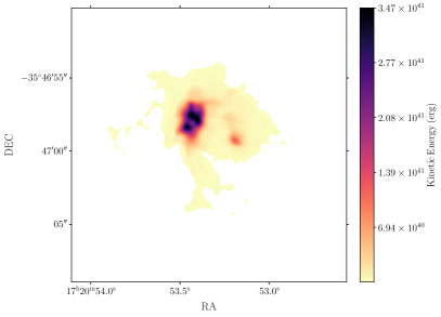
To understand the effects of the multiple physical parameters on the magnetic field, we calculate energy maps associated to turbulence (kinetic energy), gravitational, thermal, and magnetic. The kinetic energy map is estimated by computing
| (4) |
which for every pixel in the map can be approximated by
| (5) |
where is the mass per pixel obtained from the column density map, is the velocity dispersion obtained from the C33S moment 2 map where we remove the contribution from the thermal sound speed. The dispersion is calculated it as , where is the observed velocity dispersion per pixel from the C33S moment 2 map, and is the sound speed determined from the temperature model (see Figure 11), where is the Boltzmann constant. The gravitational energy is calculated as
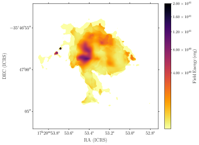
| (6) |
where is gravitational potential. This expression can also be approximated by
| (7) |
where the indices and indicate pixel positions in the map, is the mass at pixel (i,j), is the distance between the mass elements at pixels and obtained from the column density map. Although the gravitational energy is negative, we plot the absolute value in Figure 11. Note, the underlying assumption here is that the dust emission is optically thin. If the dust emission is optically thick towards the more massive cores, the estimated gravitational energy will be a lower bound. The thermal energy can be expressed as
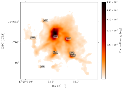
| (8) |
where we assume an ideal gas equation of state. As done before, the thermal energy per pixel can be expressed as
| (9) |
where is the number density per pixel, is the model temperature per pixel, and is the pixel volume. We calculate the pixel volume as follows, given and using , the pixel volume can be written as , where is the pixel area 444A square circumscribing each beam has 256 pixels. This yields the thermal energy per pixel as
| (10) |
The magnetic field energy density per pixel is calculated as
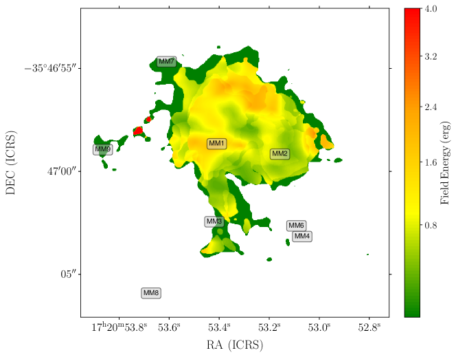
| (11) |
following the thermal energy calculation, the magnetic field energy per pixel can be estimated as
| (12) |
where is the magnetic field strength onto the plane of sky estimated using the DCF method, is the column density per pixel, and is the number density per pixel (also see Figure 11).
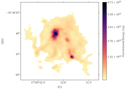
We also estimate the energy coming from the expanding MM3 cometary H II region by assuming that the emission is purely free-free which we use to estimate its thermal energy. Sadaghiani et al. (2020) obtained continuum emission with ALMA at 87.6 GHz. From these data, we estimate the size of the MM3 cometary H II by a Gaussian fit to their data which gives us a region of in size. The electron temperature, T K, and density, n cm-3 are taken from Brogan et al. (2016) simple free-free model. Thus using these values and assuming the geometrical thickness used for our density model, we obtain [ergs].
The energy balance against the magnetic field is calculated by subtracting the turbulent, thermal (both gas and UC H II), and gravitational energies to the magnetic field energy as
| (13) |
where corresponds to the combined energy in the red and blue lobes of the outflows. The results of the energy balance are listed in Table 5. We do not compute values for MM7 and MM9 because we do not have sufficient C33S coverage over these cores to obtain the velocity dispersion. From these results, it is clear that there is sufficient energy in the system to perturb the magnetic field in NGC6334I, even when considering the large uncertainties introduced by our assumptions. The differences in energy are about two orders of magnitude between the field and the combined effects of the other forces around the main cores and in the whole of NGC6334I. The gravitational energy is clearly the dominant factor in the energetics of the region, which is expected given its evolutionary stage. Nonetheless, the energy in the outflows alone are an order of magnitude larger than the magnetic energy and because the outflows might be injecting turbulence at smaller scales than gravity, the outflow feedback might be a significant factor when considering the perturbation to the magnetic field morphology. Interestingly, the energy in the cometary UC H II region, a single UC H II region, is comparable to the bulk of the thermal energy over the whole of NGC6334I. Thus, the expansion of this UC H II region might also inject additional turbulence in the gas at similar scales than the outflows. Thus, protostellar feedback maybe the dominant driver behind the injection of turbulence in NGC6334I at the scales sampled by our data. Finally, the analysis done here suggests that a magnetic field in order of milli-Gauss appears not to be a dominant factor at the core scales in NGC6334I.
4.4 Effect of the Field in the Dynamics of the Gas
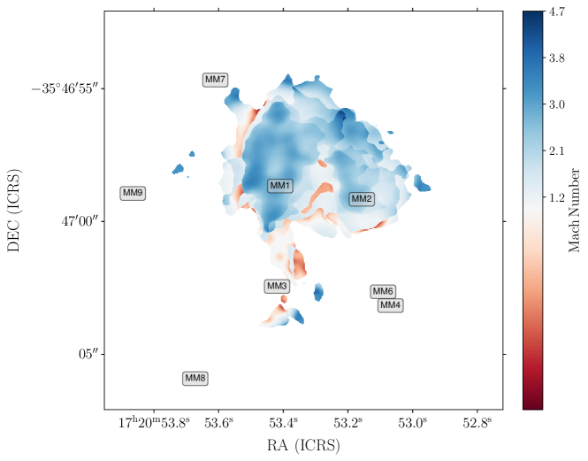
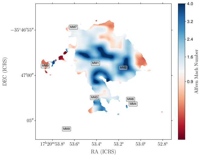
To study the effect of the magnetic field in the gas dynamics, one can start by comparing the different speeds relevant to the physical processes affecting the gas. These are the sound speed, the non-thermal velocity dispersion, obtained from optically thin molecular emission, and the Alfven speed, which we compute from estimates of the magnetic field strength. Both the velocity dispersion and the Alfven speed can be used as a proxies for the different modes of hydromagnetic waves which encompass what we understand as MHD turbulence (Mouschovias et al., 2011). Although complex in nature, in principle we can compare thermal to kinetic by computing the Mach number, or , and kinetic to magnetic by computing the Alfvenic-Mach number, or . For supersonic motions, non-thermal motions dominates the dynamics where thermal energy only becomes relevant at larger densities. However if the magnetic field is strong enough, we can have a sub-Alfenic regime, where and , which is still supersonic. In this case the magnetic field can significantly influence the dynamics through the Lorentz force (Beattie et al., 2020). In the super-Alfvenic regime where , the magnetic field plays a lesser role, but different hydromagnetic wave modes still exist which can influence the gas dynamics (Mouschovias et al., 2011).
Preliminary studies done with the SMA, Herschel, and APEX over the whole of the NGC6334 molecular cloud complex, suggested that (), but sub-Alfvenic () at resolutions of pc (Zernickel, 2015). Furthermore, Li et al. (2015) estimated the magnetic field onto the plane of the sky to conclude that the gas motions in NGC6334 are also likely to be sub-Alfvenic. Recently, ALMA observations of the NGC6334S IRDC (also part of the NGC6334 complex) used emission from H13CO+ and NH2D, to explore the non-thermal motions in the IRDC at 0.02 pc resolution with ALMA (Li et al., 2020). They found that the spatially unresolved non-thermal motions are predominantly subsonic and transonic ( 77% regions), but they made no estimations about the Alfvenic regime of the filament. The sub to transonic dominated regime in the NGC6334S IRDC suggests that the region is at a very early evolutionary stage such that the protostellar feedback-induced turbulence is small as compared to the initial turbulence (Li et al., 2020). This findings were confirmed by Liu et al. (2023a) who explored the evolution of the sonic Mach number from large scales ( pc resolution) to small scales ( pc resolution) finding the gas is mostly supersonic over 3-4 orders of magnitude in length-scales over most of NGC6334, but sub-sonic to trans-sonic in NGC6334S (the IRDC), which is consistent with what has already been observed in other IRCDs (Sanhueza et al., 2017). This IRDC is at an earlier stage of evolution respect to NGC6334I, but because is part of the same molecular complex, the cores in NGC6334S may indicate what were the initial conditions in NGC6334I.
We investigate the non-thermal motions in NGC6334I to explore how much influence the magnetic field has in the gas dynamics. To achieve this, we compute the sound speed map using the temperature model map, represented as . Employing the velocity dispersion map derived from C33S (see section 4.3), we estimate the sonic Mach number map using (see Figure 12). The Mach number map suggests that the gas is supersonic throughout most of the regions covered by the C33S emission in NGC6334I. Mach number values as high as suggests that non-thermal motions are high with turbulence being injected at the core scales to sustain the gas velocity dispersion seen here. Our values for the sonic Mach number are consistent with the previous results and with a number of other evolved high-mass star forming regions (Pattle et al., 2023; Pineda et al., 2023). To estimate the Alfvenic regime, we calculate the Alfven speed but using as an estimate of . The corresponds to the propagation speed of the transverse waves along the magnetic field lines. These motions do not involve compressions or rarefactions of the gas, meaning there is no density variation associated with these waves (different from the fast and slow magnetosonic modes). Interestingly, when using solely as the estimate, the Alfven speed does not depend on the density. This is because when introducing the original DCF equation, , into the Alfven speed expression. Because DCF assumed equipartition over the total magnetic field, a derivation of the Alfven speed based on the DCF alone is as good as the estimate and subjected to the same caveats. We show the Alfven speed map in Figure 10. Estimates of the Alfven speed from the literature are scarce. However, Roshi (2007) estimated Alfven speeds ranging between 0.7 and 4 km s-1 based on Carbon recombination line observations conducted with the Arecibo telescope. These observations targeted a set of 14 PDRs surrounding H II regions associated with high-mass star-forming regions. Liu et al. (2020) estimated Alfven speeds from their polarization mapping of the G28.34+0.06 IRDC, finding values between 0.5 to 1.5 km s-1. The values from both studies are consistent with our findings (see Figure 10).
From the Alfven speed map alone it is difficult to explore the effect of the field in the gas. To this effect, we can compute the Alfven Mach number map using (also see Figure 12). As with the Alfven speed, we note that the Alfven Mach number depends only on the dispersion of the magnetic field lines when assuming DCF, which gives . We found this approach convenient because, in principle, it allows for an estimate of this quantitative from the polarization map alone. Furthermore, the Alfven Mach number map derived here is not affected by the assumptions used to derive the temperature and density models. Furthermore, even by considering different variants of DCF, the Alfven Mach number will still strongly depend on the dispersion of the magnetic field lines. The Alfven Mach number map shown in Figure 12, strongly suggests that most of NGC6334I appears to be in trans-Alfvenic conditions () evolving to super-Alfvenic conditions () as we move into the cores. Although there are regions at the edges of the map which may be sub-Alfvenic (), their extension is small and thus inconclusive given the area covered by the C33S mask. In trans-Alfvenic conditions, the non-thermal motions can be considered to be in equipartition with the magnetic field, suggesting that the effect of the magnetic field and MHD turbulence are comparable. As density increases due to the gravitational pull, the Alfven Mach number becomes super-Alfvenic where the magnetic field is dominated by non-thermal motions. This becomes evident over the peaks with , where the exception is MM4 where the C33S emission is marginal (see Figure 6). These results agree well with the study by Pattle et al. (2023) who found that the turbulence is mostly trans-Alfvenic when statistics are compiled over many sources. The strongest peaks in the Alfven Mach number map also correlate well with the regions where we see deviations in the field orientation within scales of 1′′. Note, if the region were sudden turns are the product of projection effects, then the estimated dispersion in the field should decrease the dispersion in the field lines increasing the estimated value for Bpos at those regions. Conversely, this should also decrease the value of in those regions as well. The transition seen from trans-Alfvenic to super-Alfvenic in NGC6334I is consistent with an evolved HMSFR such NGC6334I where gravity dominates the gas dynamics and the magnetic field appears to be dynamically important only at the edges of the region. Interestingly, new high angular resolution () ALMA results from the “hourglass” magnetic field in G31.41+0.31 suggests that the gas can evolve from sub-Alfvenic to super-Alfvenic in a progression resembling NGC6334I, if we were to assume that the edges of our Alfvenic Mach number map correspond to a sub-Alfvenic regime (Beltrán et al., 2024). Now, when considering the whole NGC6334 molecular complex, exploring the Alfvenic state on NGC6334I(N), a source supposedly in an earlier stage of evolution, might show a more conclusive sub-Alfvenic to super/trans-Alfvenic condition from the outer to inner regions of the clump while the NGC6334S IRDC might likely be sub-Alfvenic. This would certainly give us significant insight about the evolutionary effect of the magnetic field over the gas dynamics in NGC6634. We leave this for future work.
5 SUMMARY AND CONCLUSIONS
We have presented sub-arcsecond resolution results from polarized dust emission and total intensity line emission observations, at 250 GHz, towards NGC6334I with ALMA. The results can be summarized as follows:
-
•
The morphology of the magnetic field onto the plane of the sky, was derived from 1.2 mm polarized dust emission under the assumption of grain alignment by magnetic fields. The magnetic field morphology is in close agreement with the ALMA results from Liu et al. (2023) taken at 1.4 mm.
-
•
Our two-epoch data over five months show no substantial change in total intensity () or linear polarization (), indicating a stable period or the end of the outburst.
-
•
To explore the effect of the four outflows detected from NGC6334I in the magnetic field, we quantified their energy by making used of the CS emission. We found that the bulk energy in the outflows is ergs.
-
•
By making used of the temperature model produced by (Liu et al., 2023), we computed energy maps for the kinetic, thermal, gravitational, and magnetic field, whose strength onto the plane of the was estimated using the DCF technique obtaining values between 1 to 11 mG with a mean magnetic field strength of 1.9 mG. When we add Zeeman measurements from OH maser observations (Hunter et al., 2018), we estimate a mean total magnetic field strength of 4 mG in agreements with others.
-
•
While the magnetic field in NGC6334I holds considerable energy, our analysis reveals that the cumulative effect of kinetic, thermal, and gravitational energies, alongside the contributions from outflows and the external pressure exerted by the surrounding cometary H II region, is capable of overpowering the magnetic field. Furthermore, the energy from the outflows alone may sufficiently disturb the field lines through the injection of turbulence at the core scales. At the same time, gravity-induced turbulence is likely to occur on larger scales. Therefore, protostellar feedback potentially emerges as the primary influence on the observed perturbations in the magnetic field’s structure across NGC6334I.
-
•
By making use the optically thin C33S emission, we computed a velocity dispersion map which we use as a proxy for the non-thermal motions. Also, by using the temperature map, we computed the thermal sound speed map and the sonic Mach number map. We found that the gas is mostly supersonic throughout NGC6334I consistent with previous findings. In the same way, we estimated the Alfven speed which we used to compute the Alfven Mach number. From the Alfven Mach number map, we found indications suggesting that gas smoothly evolve from trans-alfvenic to super-Alfvenic, with possibly sub-Alfvenic regions when we consider the outer edges of the map. This suggests that we may be seeing the progression at which the field finally gets overwhelmed by the effects of proto-stellar feedback induced turbulence and gravity in high-mass star formation.
| Region | Kinetic | Thermal Gas | Thermal H II | Gravitational | Outflow | Magnetic | Balance |
|---|---|---|---|---|---|---|---|
| (erg) | (erg) | (erg) | (erg) | (erg) | (erg) | (erg) | |
| MM1 | 0.147 | 0.025 | - | 0.762 | - | 0.016 | -0.918 |
| MM2 | 0.214 | 0.040 | - | 1.3 | - | 0.037 | -1.485 |
| MM4 | 0.013 | 0.002 | - | 0.070 | - | 0.002 | -0.082 |
| NGC6334I | 0.538 | 0.100 | 0.14 | 3.163 | 0.350 | 0.087 | -3.714 |
Note. — The energies are calculated by summing all the pixels inside the region and balance is calculated by subtracting all the energies to the magnetic field energy. The region labeled NGC6334I corresponds to the whole total intensity map. The energy in the expanding cometary UC H II region and the outflows are considered only for the bulk of NGC6334I.
Appendix A Comparison with lower frequency polarization results
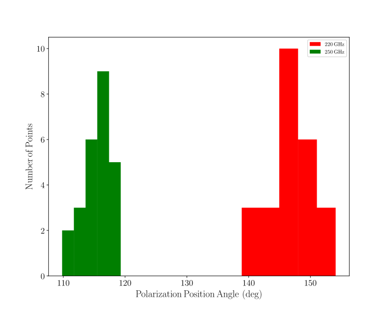
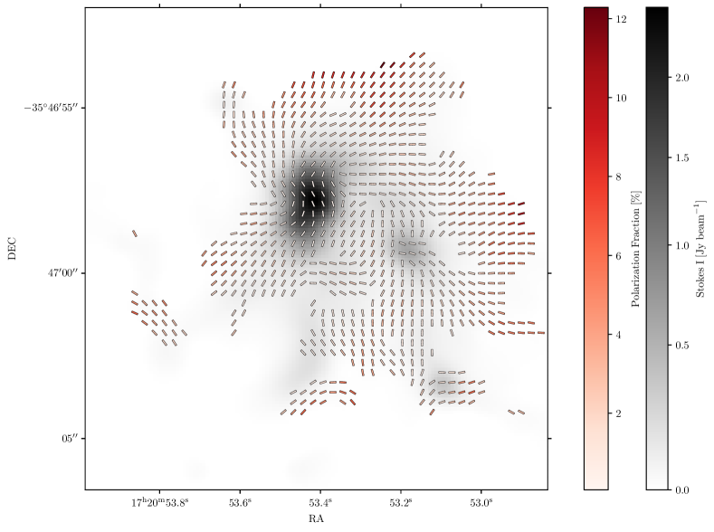
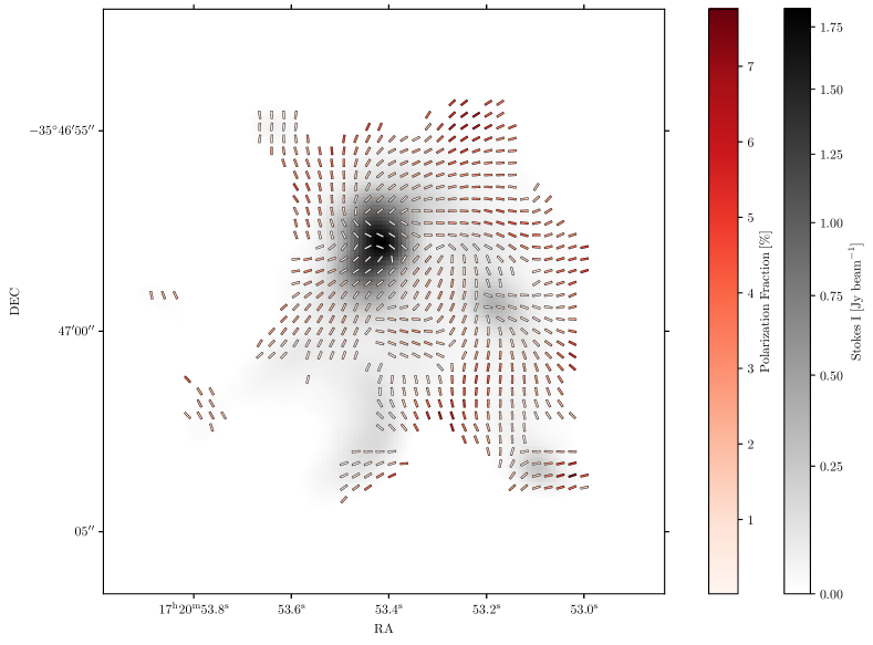
As previously mentioned, the magnetic field morphology in NGC6334I at comparable resolutions but lower frequencies, has already been explored with ALMA (Liu et al., 2023). Here we compare our results to those of Liu et al. (2023), where we see significant consistency between the field morphology obtained at 250 GHz (our data) respect to the results from 220 GHz (Liu et al., 2023). Figure 13 shows the superposed field morphologies obtained independently by both datasets. Our dataset was re-gridded to the frame and resolution of the 220 GHz data () to allow a direct comparison. When inspecting Figure 13, it is clear that the field morphologies are remarkably similar over most of the extent of the Stokes I emission. The most significant deviation between both datasets are seen at the center of the MM1 proto-cluster. The 250 GHz data shows a North-South orientation while the 220 GHz data presents a more East-West orientation. This difference in the field morphology is significant (, see Figure 14) when compared to the rest of the map where the pseudo-vectors agree quite well. To explore if this is the result of calibration uncertainties, Figure 15 shows the derived magnetic field morphology at both frequencies, but now the pseudo-vectors are colored to indicate the level of fractional polarization (the fractional polarization maps have cutoff in Stokes I and a coarser sampling rate). At center, where the Stokes I peaks and the difference in angle is the largest, the range of fractional polarization is between 0.1% and 0.15% in both datasets. Although this range is close to the polarization calibrationa accuracy of ALMA (0.1 % Cortes et al., 2023), it is sufficently large to suggests that the difference might be real. Given the current datasets, it is difficult to ascertain what is the cause of such difference, particularly considering the excellent overall agreement between them throughout the region where both datasets are separated by just 30 GHz. Polarized emission by self-scattering appears implausible as an explanation (as discussed in section 3.3). High resolution ALMA observations in full Stokes should be conducted to explore this discrepancy further.
Appendix B The Magnetic Field Dispersion Map
To estimate the magnetic field strength onto the plane of the sky using DCF, estimating the dispersion in the polarization position angle is critical. Because we assume flux freezing, the local dispersion in the field lines is produced by collisions between the charge carriers and the neutrals. These collisions perturb the mean field yielding deviations in its local direction, which we understand as the dispersion. The dispersion is an statistical quantity and thus we will use statistical arguments to estimate its value. Because we are interested in obtaining a map, we make use of a moving window to calculate the standard deviation using semicircular statistics. To define the size of the window, we assume that the angles follow a Gaussian distribution. Although Gaussian distribution is a “usual” assumption in astronomy, its usage here can be justified from the point of view of the central limit theorem. If we assume that the perturbations over the field lines are local then each independent point in the map can be considered as a random variable following it own distribution due to the actions of the local turbulence. In the limit of large numbers distribution of the mean of all of independent points follows a Gaussian distribution. Moreover, local turbulence can also be modelled using a Gaussian distribution as done by Houde et al. (2009) in the their ADF approximation which also provides an alternative method to derive the dispersion in the field. Therefore and under this consideration, we use the standard error of the mean as:
| (B1) |
where is the population standard deviation (unknown but can be estimated from the sample), and is the population size. For a 95% confidence interval (which might be akin to a 95% credible interval in a Bayesian context, although the interpretation is different), the margin of error is
| (B2) |
If we assume a margin of error to be within 5∘, then gives the number of independent points required for an error of 5∘, where is the estimate of . To estimate , we take the mean of the standard deviation over regions in the map where the field appears to be coherent, by visual inspection, on scales of . This give us an initial population standard deviation estimate of . Thus, we obtain independent points as the required number (beams), which when assuming Nyquist sampling for the beam, we obtain a window of in size. The final dispersion map is calculated as:
| (B3) |
where represents the error in the polarization position angle in an ALMA map, with and being the rms and the polarization intensity respectively (Hull et al., 2020).
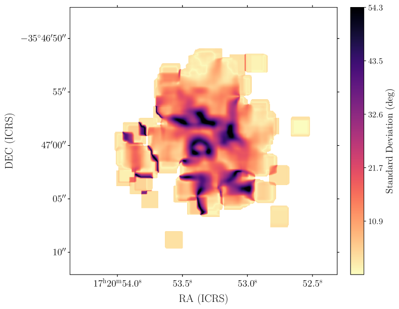
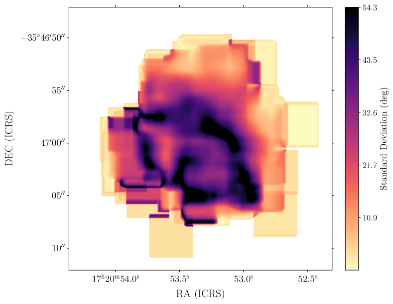
Although the choice of may appear arbitrary, we found it to be a good compromise. A smaller window results in a larger error, while a larger window not only smooths out the map but also biases regions where the field appears smooth. This is because it propagates larger deviations in the field lines seen in the regions where the field has turns; regions where DCF is likely not fully applicable. An example of this can be seen in Figure 17 where we show a dispersion map using a window of 4′′. This windows size has an estimated error of , but the spatial distribution of dispersions values over is significantly larger than our current choice (see Figure 16). Analysis of the DCF technique done by comparing with simulations, suggest that the applicability of DCF decreases with dispersion values over (see Crutcher et al., 2004, and references therein ). Table 6 shows the error estimates for the position angle dispersion for window sizes ranging from to .
Finally, it is important to note that the maximum value for the standard deviation under semicircular statistics is . This is because, the maximum dispersion is achieved when we have a uniform distribution over the semicircle with a probability density function of which yields .
| Window Size | Number of Beams | Dispersion Error |
|---|---|---|
| 1.0 | 6 | 8 |
| 1.5 | 16 | 5 |
| 2.0 | 25 | 4 |
| 2.5 | 40 | 3 |
| 3.0 | 56 | 3 |
| 4.0 | 100 | 2 |
| 5.0 | 156 | 2 |
| 6.0 | 225 | 1 |
| 7.0 | 306 | 1 |
Note. — The errors where rounded to a single integer for consistency and the number of beams assume Nyquist sampling.
Appendix C Simple Error Estimation for DCF
Although a number of caveats constrain the interpretation of our result from DCF (see section 4.2.2), here we attempt to quatify these uncertainties by employing simple error propagation to estimate an error for . The expression that we used for DCF is given by equation 3, which under simple error propagation becomes,
| (C1) |
where , , and are the uncertainties in the number density, velocity dispersion, and position angle dispersion respectively. The most difficult quantity to estimate is the number density error, because of the uncertainties previously mentioned. We attempt to circumvent this by calculating the mean absolute error between our model and the values derived by Brogan et al. (2016). Because both data sets come from ALMA observations from the same source, a number of systematics can be removed by taking the difference between their values and our model. In this way, the mean absolute error can be calculated as,
| (C2) |
where corresponds to the number density estimate done by Brogan et al. (2016) on source , is the the number density estimate from our model over source , and is the total number of sources. In this way, we obtained cm-3 as the number density error. The uncertainty in the velocity dispersion is estimated by the resolution used in the spectral setup of the C33S line, or km s-1, while the error estimate for the position angle dispersion is (see appendix B also for a discussion about the impact a different windows sizes in the error estimate). With all of these values we obtain a mean error estimate, mG after rounding, which yields mG. From the values of obtained by Hunter et al. (2018), we estimate an error also of 1 mG which after adding them in quadrature and rounding we obtained mG.
Facilities: ALMA.
Acknowledgments
P.C.C. acknowledges publication and travel support from ALMA, NAOJ, and NRAO. This work was supported by the NAOJ Research Coordination Committee, NINS (NAOJ-RCC-2202-0401). P.S. was partially supported by a Grant-in-Aid for Scientific Research (KAKENHI Number JP22H01271 and JP23H01221) of JSPS. J.M.G. acknowledges support by the grant PID2020-117710GB-I00 (MCI-AEI-FEDER, UE). This work is also partially supported by the program Unidad de Excelencia María de Maeztu CEX2020-001058-M. L.A.Z acknowledges financial support from CONACyT-280775 and UNAM-PAPIITIN110618 grants, Mexico. A.S.-M. acknowledges support from the RyC2021-032892-I grant funded by MCIN/AEI/10.13039/501100011033 and by the European Union ‘Next GenerationEU’/PRTR, as well as the program Unidad de Excelencia María de Maeztu CEX2020-001058-M, and support from the PID2020-117710GB-I00 (MCI-AEI-FEDER, UE). This work was supported by the NAOJ Research Coordination Committee, NINS (NAOJ-RCC-2202-0401). This paper makes use of the following ALMA data: ADS/JAO.ALMA#2018.1.00105.S. ALMA is a partnership of ESO (representing its member states), NSF (USA) and NINS (Japan), together with NRC (Canada), MOST and ASIAA (Taiwan), and KASI (Republic of Korea), in cooperation with the Republic of Chile. The Joint ALMA Observatory is operated by ESO, AUI/NRAO and NAOJ. The National Radio Astronomy Observatory is a facility of the National Science Foundation operated under cooperative agreement by Associated Universities, Inc.
References
- Arzoumanian et al. (2011) Arzoumanian, D., André, P., Didelon, P., et al. 2011, A&A, 529, L6, doi: 10.1051/0004-6361/201116596
- Arzoumanian et al. (2021) Arzoumanian, D., Furuya, R. S., Hasegawa, T., et al. 2021, A&A, 647, A78, doi: 10.1051/0004-6361/202038624
- Astropy Collaboration et al. (2018) Astropy Collaboration, Price-Whelan, A. M., Sipőcz, B. M., et al. 2018, AJ, 156, 123, doi: 10.3847/1538-3881/aabc4f
- Bachiller & Cernicharo (1990) Bachiller, R., & Cernicharo, J. 1990, A&A, 239, 276
- Beattie et al. (2020) Beattie, J. R., Federrath, C., & Seta, A. 2020, MNRAS, 498, 1593, doi: 10.1093/mnras/staa2257
- Beltrán et al. (2019) Beltrán, M. T., Padovani, M., Girart, J. M., et al. 2019, A&A, 630, A54, doi: 10.1051/0004-6361/201935701
- Beltrán et al. (2024) Beltrán, M. T., Padovani, M., Galli, D., et al. 2024, arXiv e-prints, arXiv:2404.10347, doi: 10.48550/arXiv.2404.10347
- Beuther et al. (2008) Beuther, H., Walsh, A. J., Thorwirth, S., et al. 2008, A&A, 481, 169, doi: 10.1051/0004-6361:20079014
- Beuther et al. (2020) Beuther, H., Soler, J. D., Linz, H., et al. 2020, ApJ, 904, 168, doi: 10.3847/1538-4357/abc019
- Beuther et al. (2023) Beuther, H., Gieser, C., Soler, J. D., et al. 2023, arXiv e-prints, arXiv:2311.11874, doi: 10.48550/arXiv.2311.11874
- Brogan et al. (2016) Brogan, C. L., Hunter, T. R., Cyganowski, C. J., et al. 2016, ApJ, 832, 187, doi: 10.3847/0004-637X/832/2/187
- Brogan et al. (2018) —. 2018, ApJ, 866, 87, doi: 10.3847/1538-4357/aae151
- Burns et al. (2023) Burns, R. A., Uno, Y., Sakai, N., et al. 2023, Nature Astronomy, 7, 557, doi: 10.1038/s41550-023-01899-w
- Bustreel et al. (1979) Bustreel, R., Demuynck-Marlière, D., Destombes, J., & Journel, G. 1979, Journal of Chemical Physics Letters, 67, 178
- CASA Team et al. (2022) CASA Team, Bean, B., Bhatnagar, S., et al. 2022, PASP, 134, 114501, doi: 10.1088/1538-3873/ac9642
- Caswell et al. (2011) Caswell, J. L., Kramer, B. H., & Reynolds, J. E. 2011, MNRAS, 414, 1914, doi: 10.1111/j.1365-2966.2011.18510.x
- Chandrasekhar & Fermi (1953) Chandrasekhar, S., & Fermi, E. 1953, ApJ, 118, 113
- Chibueze et al. (2014) Chibueze, J. O., Omodaka, T., Handa, T., et al. 2014, ApJ, 784, 114, doi: 10.1088/0004-637X/784/2/114
- Cho & Yoo (2016) Cho, J., & Yoo, H. 2016, ApJ, 821, 21, doi: 10.3847/0004-637X/821/1/21
- Ciolek & Mouschovias (1994) Ciolek, G. E., & Mouschovias, T. C. 1994, ApJ, 425, 142, doi: 10.1086/173971
- Cortes et al. (2023) Cortes, P., Vlahakis, C., Hales, A., et al. 2023, ALMA Cycle 10 Technical Handbook, doi: 10.5281/zenodo.7822943
- Cortes et al. (2005) Cortes, P. C., Crutcher, R. M., & Watson, W. D. 2005, ApJ, 628, 780, doi: 10.1086/430815
- Cortes et al. (2016) Cortes, P. C., Girart, J. M., Hull, C. L. H., et al. 2016, ApJ, 825, L15, doi: 10.3847/2041-8205/825/1/L15
- Cortes et al. (2019) Cortes, P. C., Hull, C. L. H., Girart, J. M., et al. 2019, ApJ, 884, 48, doi: 10.3847/1538-4357/ab378d
- Cortes et al. (2021a) Cortes, P. C., Le Gouellec, V. J. M., Hull, C. L. H., et al. 2021a, ApJ, 907, 94, doi: 10.3847/1538-4357/abcafb
- Cortés et al. (2021b) Cortés, P. C., Sanhueza, P., Houde, M., et al. 2021b, ApJ, 923, 204, doi: 10.3847/1538-4357/ac28a1
- Cragg et al. (2002) Cragg, D. M., Sobolev, A. M., & Godfrey, P. D. 2002, MNRAS, 331, 521, doi: 10.1046/j.1365-8711.2002.05226.x
- Crutcher & Kemball (2019) Crutcher, R. M., & Kemball, A. J. 2019, Frontiers in Astronomy and Space Sciences, 6, 66, doi: 10.3389/fspas.2019.00066
- Crutcher et al. (2004) Crutcher, R. M., Nutter, D. J., Ward-Thompson, D., & Kirk, J. M. 2004, ApJ, 600, 279
- Davis (1951) Davis, L. 1951, Phys. Rev., 81, 890, doi: 10.1103/PhysRev.81.890.2
- Falceta-Gonçalves et al. (2008) Falceta-Gonçalves, D., Lazarian, A., & Kowal, G. 2008, ApJ, 679, 537, doi: 10.1086/587479
- Feddersen et al. (2020) Feddersen, J. R., Arce, H. G., Kong, S., et al. 2020, ApJ, 896, 11, doi: 10.3847/1538-4357/ab86a9
- Fernández-López et al. (2021) Fernández-López, M., Sanhueza, P., Zapata, L. A., et al. 2021, ApJ, 913, 29, doi: 10.3847/1538-4357/abf2b6
- Girart et al. (2013) Girart, J. M., Frau, P., Zhang, Q., et al. 2013, ApJ, 772, 69, doi: 10.1088/0004-637X/772/1/69
- Girart et al. (2006) Girart, J. M., Rao, R., & Marrone, D. P. 2006, Science, 313, 812, doi: 10.1126/science.1129093
- Heitsch et al. (2001) Heitsch, F., Zweibel, E. G., Mac Low, M.-M., Li, P., & Norman, M. L. 2001, ApJ, 561, 800, doi: 10.1086/323489
- Hildebrand (1983) Hildebrand, R. H. 1983, QJRAS, 24, 267
- Houde et al. (2009) Houde, M., Vaillancourt, J. E., Hildebrand, R. H., Chitsazzadeh, S., & Kirby, L. 2009, ApJ, 706, 1504, doi: 10.1088/0004-637X/706/2/1504
- Hull & Plambeck (2015) Hull, C. L. H., & Plambeck, R. L. 2015, Journal of Astronomical Instrumentation, 4, 1550005, doi: 10.1142/S2251171715500051
- Hull et al. (2014) Hull, C. L. H., Plambeck, R. L., Kwon, W., et al. 2014, ApJS, 213, 13, doi: 10.1088/0067-0049/213/1/13
- Hull et al. (2017) Hull, C. L. H., Girart, J. M., Tychoniec, Ł., et al. 2017, ApJ, 847, 92, doi: 10.3847/1538-4357/aa7fe9
- Hull et al. (2020) Hull, C. L. H., Cortes, P. C., Gouellec, V. J. M. L., et al. 2020, PASP, 132, 094501, doi: 10.1088/1538-3873/ab99cd
- Hunter et al. (2014) Hunter, T. R., Brogan, C. L., Cyganowski, C. J., & Young, K. H. 2014, ApJ, 788, 187, doi: 10.1088/0004-637X/788/2/187
- Hunter et al. (2017) Hunter, T. R., Brogan, C. L., MacLeod, G., et al. 2017, ApJ, 837, L29, doi: 10.3847/2041-8213/aa5d0e
- Hunter et al. (2018) Hunter, T. R., Brogan, C. L., MacLeod, G. C., et al. 2018, ApJ, 854, 170, doi: 10.3847/1538-4357/aaa962
- Hunter et al. (2021) Hunter, T. R., Brogan, C. L., Buizer, J. M. D., et al. 2021, The Astrophysical Journal Letters, 912, L17, doi: 10.3847/2041-8213/abf6d9
- Kataoka et al. (2016) Kataoka, A., Tsukagoshi, T., Momose, M., et al. 2016, ApJ, 831, L12, doi: 10.3847/2041-8205/831/2/L12
- Koch et al. (2012a) Koch, P. M., Tang, Y.-W., & Ho, P. T. P. 2012a, ApJ, 747, 79, doi: 10.1088/0004-637X/747/1/79
- Koch et al. (2012b) —. 2012b, ApJ, 747, 80, doi: 10.1088/0004-637X/747/1/80
- Koch et al. (2013) —. 2013, ApJ, 775, 77, doi: 10.1088/0004-637X/775/1/77
- Koch et al. (2018) Koch, P. M., Tang, Y.-W., Ho, P. T. P., et al. 2018, ApJ, 855, 39, doi: 10.3847/1538-4357/aaa4c1
- Koch et al. (2022) —. 2022, ApJ, 940, 89, doi: 10.3847/1538-4357/ac96e3
- Lazarian & Hoang (2007) Lazarian, A., & Hoang, T. 2007, MNRAS, 378, 910, doi: 10.1111/j.1365-2966.2007.11817.x
- Lazarian et al. (2022) Lazarian, A., Yuen, K. H., & Pogosyan, D. 2022, ApJ, 935, 77, doi: 10.3847/1538-4357/ac6877
- Li et al. (2015) Li, H., Li, D., Qian, L., et al. 2015, ApJS, 219, 20, doi: 10.1088/0067-0049/219/2/20
- Li et al. (2010) Li, H.-b., Houde, M., Lai, S.-p., & Sridharan, T. K. 2010, ApJ, 718, 905, doi: 10.1088/0004-637X/718/2/905
- Li et al. (2020) Li, S., Zhang, Q., Liu, H. B., et al. 2020, ApJ, 896, 110, doi: 10.3847/1538-4357/ab84f1
- Liu et al. (2021) Liu, J., Zhang, Q., Commerçon, B., et al. 2021, ApJ, 919, 79, doi: 10.3847/1538-4357/ac0cec
- Liu et al. (2020) Liu, J., Zhang, Q., Qiu, K., et al. 2020, ApJ, 895, 142, doi: 10.3847/1538-4357/ab9087
- Liu et al. (2023a) Liu, J., Zhang, Q., Koch, P. M., et al. 2023a, ApJ, 945, 160, doi: 10.3847/1538-4357/acb540
- Liu et al. (2023b) Liu, J., Zhang, Q., Liu, H. B., et al. 2023b, ApJ, 949, 30, doi: 10.3847/1538-4357/acc4c0
- Liu et al. (2023) Liu, J., Zhang, Q., Koch, P. M., et al. 2023, The Astrophysical Journal, 945, 160, doi: 10.3847/1538-4357/acb540
- MacLeod et al. (2018) MacLeod, G. C., Smits, D. P., Goedhart, S., et al. 2018, MNRAS, 478, 1077, doi: 10.1093/mnras/sty996
- Martín et al. (2019) Martín, S., Martín-Pintado, J., Blanco-Sánchez, C., et al. 2019, A&A, 631, A159, doi: 10.1051/0004-6361/201936144
- McCutcheon et al. (2000) McCutcheon, W. H., Sandell, G., Matthews, H. E., et al. 2000, MNRAS, 316, 152, doi: 10.1046/j.1365-8711.2000.03487.x
- Mouschovias et al. (2011) Mouschovias, T. C., Ciolek, G. E., & Morton, S. A. 2011, MNRAS, 415, 1751, doi: 10.1111/j.1365-2966.2011.18817.x
- Myers et al. (2024) Myers, P. C., Stephens, I. W., & Coudé, S. 2024, ApJ, 962, 64, doi: 10.3847/1538-4357/ad1596
- Ossenkopf & Henning (1994) Ossenkopf, V., & Henning, T. 1994, A&A, 291, 943
- Ossenkopf-Okada et al. (2016) Ossenkopf-Okada, V., Csengeri, T., Schneider, N., Federrath, C., & Klessen, R. S. 2016, A&A, 590, A104, doi: 10.1051/0004-6361/201628095
- Palau et al. (2021) Palau, A., Zhang, Q., Girart, J. M., et al. 2021, The Astrophysical Journal, 912, 159, doi: 10.3847/1538-4357/abee1e
- Pattle et al. (2023) Pattle, K., Fissel, L., Tahani, M., Liu, T., & Ntormousi, E. 2023, in Astronomical Society of the Pacific Conference Series, Vol. 534, Protostars and Planets VII, ed. S. Inutsuka, Y. Aikawa, T. Muto, K. Tomida, & M. Tamura, 193, doi: 10.48550/arXiv.2203.11179
- Pineda et al. (2023) Pineda, J. E., Arzoumanian, D., Andre, P., et al. 2023, in Astronomical Society of the Pacific Conference Series, Vol. 534, Protostars and Planets VII, ed. S. Inutsuka, Y. Aikawa, T. Muto, K. Tomida, & M. Tamura, 233, doi: 10.48550/arXiv.2205.03935
- Rao et al. (1998) Rao, R., Crutcher, R. M., Plambeck, R. L., & Wright, M. C. H. 1998, ApJ, 502, L75+
- Roshi (2007) Roshi, D. A. 2007, ApJ, 658, L41, doi: 10.1086/513465
- Sadaghiani et al. (2020) Sadaghiani, M., Sánchez-Monge, Á., Schilke, P., et al. 2020, A&A, 635, A2, doi: 10.1051/0004-6361/201935699
- Sandell (2000) Sandell, G. 2000, A&A, 358, 242
- Sanhueza (2024) Sanhueza, P. 2024, ApJ
- Sanhueza et al. (2017) Sanhueza, P., Jackson, J. M., Zhang, Q., et al. 2017, ApJ, 841, 97, doi: 10.3847/1538-4357/aa6ff8
- Sanhueza et al. (2021) Sanhueza, P., Girart, J. M., Padovani, M., et al. 2021, ApJ, 915, L10, doi: 10.3847/2041-8213/ac081c
- Savitzky & Golay (1964) Savitzky, A., & Golay, M. J. E. 1964, Analytical Chemistry, 36, 1627
- Skalidis & Tassis (2021) Skalidis, R., & Tassis, K. 2021, A&A, 647, A186, doi: 10.1051/0004-6361/202039779
- Tang et al. (2009) Tang, Y.-W., Ho, P. T. P., Girart, J. M., et al. 2009, ApJ, 695, 1399, doi: 10.1088/0004-637X/695/2/1399
- Tazaki et al. (2017) Tazaki, R., Lazarian, A., & Nomura, H. 2017, ApJ, 839, 56, doi: 10.3847/1538-4357/839/1/56
- Wardle & Kronberg (1974) Wardle, J. F. C., & Kronberg, P. P. 1974, ApJ, 194, 249, doi: 10.1086/153240
- Yu et al. (2020) Yu, H. Z., Zhang, J. S., Henkel, C., et al. 2020, ApJ, 899, 145, doi: 10.3847/1538-4357/aba8f1
- Zernickel (2015) Zernickel, A. 2015, PhD thesis, University of Cologne, Institute for Physics
- Zernickel et al. (2012) Zernickel, A., Schilke, P., Schmiedeke, A., et al. 2012, A&A, 546, A87, doi: 10.1051/0004-6361/201219803
- Zhang et al. (2014a) Zhang, B., Moscadelli, L., Sato, M., et al. 2014a, ApJ, 781, 89, doi: 10.1088/0004-637X/781/2/89
- Zhang et al. (2005) Zhang, Q., Hunter, T. R., Brand, J., et al. 2005, ApJ, 625, 864, doi: 10.1086/429660
- Zhang et al. (2001) —. 2001, ApJ, 552, L167, doi: 10.1086/320345
- Zhang et al. (2014b) Zhang, Q., Qiu, K., Girart, J. M., et al. 2014b, ApJ, 792, 116, doi: 10.1088/0004-637X/792/2/116
- Zhang et al. (2014c) —. 2014c, ApJ, 792, 116, doi: 10.1088/0004-637X/792/2/116
- Zhang et al. (2016) Zhang, Y., Arce, H. G., Mardones, D., et al. 2016, ApJ, 832, 158, doi: 10.3847/0004-637X/832/2/158