Modelling the evolution of the Galactic disc scale height traced by open clusters

Abstract

Context. The scale height of the spatial distribution of open clusters (OCs) in the Milky Way exhibits a well known increase with age which is usually interpreted as evidence for dynamical heating of the disc or of the disc having been thicker in the past.

Aims. We address the increase of the scale height with age of the OC population from a different angle. We propose that the apparent thickening of the disc can be largely explained as a consequence of a stronger disruption of OCs near the Galactic plane by disc phenomena, namely encounters with giant molecular clouds (GMCs).

Methods. We present a computational model that forms OCs with different initial masses and follows their orbits while subjecting them to different disruption mechanisms. To setup the model and infer its parameters, we use and analyse a Gaia-based OC catalogue (Dias et al. 2021). We investigate both the spatial and age distributions of the OC population and discuss the completeness of the sample. The simulation results are then compared to the observations.

Results. Consistent with previous studies, the observations reveal that the SH of the spatial distribution of OCs increases with age. We find that it is very likely that the OC sample is incomplete even for the solar neighbourhood. The model simulations successfully reproduce the SH increase with age and the total number of OCs that survive with age up to 1 Gyr. For older OCs, the predicted SH from the model starts deviating from the observations, although remaining within the uncertainties of the observations. This can be related with effects of incompleteness and/or simplifications in the model.

Conclusions. A selective disruption of OCs near the galactic plane through GMC encounters is able to explain the SH evolution of the OC population.

1 Introduction

Understanding the evolution of galaxies involves tracking their morphological changes and identifying the mechanisms driving these transformations. The Milky Way’s thin disc, which hosts most of the stars in the Galaxy, has been continuously forming stars for more than ten billion years. This activity has led to a complex history of stellar dynamics interwoven with interactions with the interstellar medium, shaping the disc throughout its existence.

To a good approximation, the vertical number-density of stars in the Galactic disc decreases exponentially with distance from the disc’s plane (Bahcall & Soneira 1980). The exponential decrease is characterised by the decay factor, referred to as the disc scale-height (SH), which parameterises the thickness of the disc. Different populations of objects may display different vertical distributions. For instance, the distribution of stars can have a SH from $\sim 40\pm 7$ pc at log(age) $\sim 7.5-7.7$ up to 211 $\pm 13$ pc at log(age) $\sim 9.3-9.5$ (Mazzi et al. 2024). Although the thickness of the disc can be studied using various types of objects, such as stars of different spectral types, open clusters (OCs) are often used as disc probes due to the advantages that they provide from an observational standpoint (e.g Moitinho 2010). In particular, OC ages can be determined with an accuracy out of reach for most stars, which allows a direct inspection of specific times in the evolution of the Galaxy. The SH of the spatial distribution of OCs in the Milky Way exhibits a well known increase with age and has been discussed multiple times in past studies (e.g Lynga 1982, 1985; Janes & Phelps 1994; Bonatto et al. 2006; Buckner & Froebrich 2014; Cantat-Gaudin et al. 2020; Joshi & Malhotra 2023). Table 1 shows the SHs obtained for different ages in a non exhaustive list of previous studies. The table, which includes SH determinations derived from data obtained by the Gaia mission (Gaia Collaboration et al. 2016, 2018, 2021) as well as from before Gaia, clearly shows that the OC SH increase with age is a well established observational result.

Table 1: Scale height of the OC distributions of different age groups from previous studies.

Reference	Age (Myr)	S${}_{\text{H}}$ (pc)
Lynga (1985)	$<100$	60
	100 - 1000	80
	$>$ 1000	200
Janes & Phelps (1994)	Young	55
	Old	375
Bonatto et al. (2006)	$<200$	47.9 $\pm$ 2.8
	200 - 1000	149.8 $\pm$ 26.3
	$>1000$	$\infty$
Buckner & Froebrich (2014)	1	40
	1000	75
	3500	550
Cantat-Gaudin et al. (2020)	100	74 $\pm$ 5
	1000	142 $\pm$ 7
Hao et al. (2021)	$<20$	70.5 $\pm$ 2.3
	20 - 100	87.4 $\pm$ 3.6
Joshi & Malhotra (2023)	$<20$	80.8 $\pm$ 8.0
	20 - 700	96.4 $\pm$ 1.9
	700 - 2000	294.7 $\pm$ 19.5

Because OCs are bound groups of stars with different masses immersed in the Galactic potential, there is a variety of both internal and external factors that contribute to their evolution and, ultimately, dissolution. Thus, studying the evolution of the OC population, particularly its vertical distribution, is key to understand the underlying mechanisms that shape the structure of the MW and its evolution.

The increase of the SH with age of the OC population is usually interpreted in a way similar to that of the SH evolution of the stellar population: as evidence for the disc having been thicker in the past (Janes & Phelps 1994), or to dynamical heating of the disc due to scattering events, such as interactions with the spiral arms and giant molecular clouds (GMCs)(Gustafsson et al. 2016; Buckner & Froebrich 2014). However, as pointed out by Friel (1995), the encounters leading to such orbit perturbations could also disrupt the clusters themselves. Moreover, (Lamers & Gieles 2006) showed that encounters with GMCs may be the main mechanism responsible for the disruption of OCs in the solar neighbourhood. On the kinematic side, Tarricq et al. (2021) studied the dependency of the velocity dispersion with age in the form of a power-law: $\sigma_{V}=\tau^{\beta}$, where they estimate $\beta_{Z}=0.19^{+0.03}_{-0.03}$. As they suggest, even though these mechanisms are likely the main cause for the scattering of the field stars, a small $\beta_{Z}$ could indicate they may not be as efficient in scattering OCs. In any case, these arguments point out possible factors, but no actual astrophysical modelling has been published to reproduce the SH evolution of the OC distribution.

In this context, we follow the suggestion of Moitinho (2010) and address the increase of the SH of the OC population with age from a different angle: that the increase of the SH might be a consequence of a stronger disruption near the Galactic plane (GP) due to disc phenomena such as encounters with GMCs. The OCs formed at larger distances to the GP are likely to survive longer, not only because they spend most of their lifetimes at larger distances to the plane, but also cross it with higher velocities, having less time to be affected the disruption mechanisms. As the time passes, the distribution is gradually trimmed at lower heights, resulting in a flattening of the height distribution and an apparent increase of the SH with time. We present a dynamical model that follows the orbits of OCs and includes their disruption due to interactions with the disc and mass loss due to stellar evolution and evaporation.

This paper is structured as follows: In Sect. 2 we present the observational sample of OCs and discuss statistical properties that are relevant for this study, such as the completeness of the sample, as well as the spatial and age distributions. In Sect. 3 we present the proposed model and how we setup the parameters related to the integration of the orbits, the initial masses of the OCs and the mechanisms of disruption. Sect. 4 provides a more in depth analysis of the parameter space where we infer the free parameters of the model by grid-searching optimal solutions. In Sect. 5 we discuss the obtained results. Final considerations and conclusions of this study are presented in Sect. 6.

2 Observational Data

2.1 Overview

The high-precision astrometric and photometric data from Gaia mission has allowed significant progress in building an observational base of OCs. It has brought the discovery of hundreds of new OCs (e.g. Castro-Ginard et al. 2018; Liu & Pang 2019; Cantat-Gaudin et al. 2019; Sim et al. 2019; Ferreira et al. 2020; Cantat-Gaudin et al. 2020, 2018b; Jaehnig et al. 2021; Hunt & Reffert 2023), the identification of their members and the systematic determination of their fundamental parameters (e.g. Cantat-Gaudin et al. 2018a; Bossini et al. 2019; Carrera et al. 2019; Monteiro & Dias 2019; Cantat-Gaudin et al. 2020; Monteiro et al. 2020; Hunt & Reffert 2023).

The OCs parameters used in this study are from the catalogue of Dias et al. (2021), which uses the data from Gaia Data Release 2 (DR2) and contains a total of 1743 clusters along with their ages, distances, proper motions, metallicities and many others properties. The individual stellar memberships are collected from other studies (full list in Dias et al. 2021). This catalogue provides homogeneous determinations of ages and distances, among other parameters, which were obtained using the same isochrone set and fitting method, as described in Monteiro et al. (2017) and Monteiro et al. (2020).

To study the dependency of SH with age, we will proceed similarly to Janes & Phelps (1994); Bonatto et al. (2006); Joshi & Malhotra (2023) and split the OCs sample in different age groups. Thanks to the larger number of OC parameters available for this study, we include an additional age group. Table 2 shows the selected age intervals for each group with the corresponding sample sizes.

Table 2: Considered age groups for the sample of OCs catalogued in Dias et al. (2021).

	Age (Myr)	Sample Size
Young	0 $<$ Age $\leq 200$	969
Intermediate Young	200 $<$ Age $\leq 500$	333
Intermediate Old	500 $<$ Age $\leq 1000$	250
Old	Age $>1000$	191
All	- -	1743

2.2 Distribution on the Galactic Plane and Completeness

We now proceed to characterise our observational sample, starting by considering the sample completeness. The completeness of the OCs census has been discussed multiple times in the literature with different studies claiming that the sample of OCs is complete in the solar neighbourhood up to distances of $\sim 1$ kpc (Kharchenko et al. 2013; Piskunov et al. 2006; Buckner & Froebrich 2014) from the Sun, some even suggesting greater distances of $\sim$ 2-3 kpc (Joshi 2005), although those claims had been questioned by Moitinho (2010). The recent avalanche of OC discoveries mentioned above has clearly shown assumptions of completeness may not be correct, even in the solar neighbourhood. To assess the dependence of completeness on distance, we split the OCs in sub-samples, considering 3 cylindrical cuts with radii of 1.00, 1.75 and 2.50 kpc.

Figure 1 shows, for each age group, the projected spatial distribution of OCs on the GP using the galactocentric coordinate frame from astropy SkyCoord (Astropy Collaboration et al. 2022). The Sun is located at (X, Y) = (-8.122, 0) kpc, with the angular coordinate corresponding to the Galactic longitude. Dashed circumferences represent the cylindrical cuts considered. The plots also include kernel density estimations (KDE) of the number-density of OCs on the XY plane, using a Gaussian kernel with a bandwidth of 650 pc. The choice of a large bandwidth was made within the context of addressing incompleteness rather than emphasising local structures. The plots reveal that the sample of OCs does not exhibit an homogeneous spatial distribution on the plane. A systematic decrease of the number of observed OCs with the distance to the Sun is well seen.

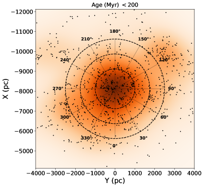
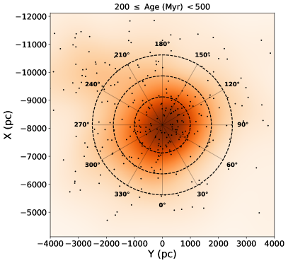
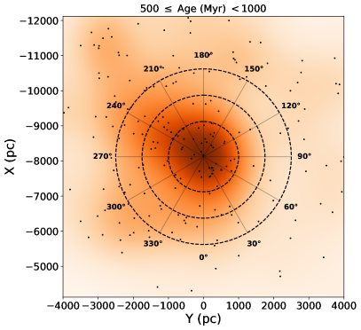
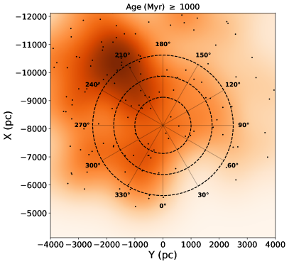
Figure 1: Distribution of OCs catalogued in Dias et al. (2021), projected on the GP, in galactocentric coordinates, for the different age groups used in the study. The Sun is located at (-8.122, 0) kpc. The concentric circumferences represent the radii of the cylindrical cuts considered: 1.00, 1.75 and 2.50 kpc. The colour scale encodes the number-density of OCs on the plane, with darker tones representing higher density.

Assuming that our position in the Galaxy is not special, for a complete sample the surface density of the number of OCs should remain roughly constant in our neighbourhood. Figure 2 shows the surface density, in concentric rings, for different radial heliocentric distances and for the considered age groups. The initial bins correspond to circles with a radius of 0.4 kpc and subsequent rings then increase the radius by 0.4 kpc for age groups younger than 1000 Myr, and 0.8 kpc for the older age group. The curves are normalised so that the maximum surface density equals unity, for each age group. With exception of the old OCs, all age groups exhibit similar decline of the surface density. The trends observed in other observational catalogues are similar to those displayed in age groups with ages $<1000$ Myr (see Buckner & Froebrich 2014, figure 1). This is a strong indication that the sample of OCs is not complete for distances $<1.5$ kpc or even $1$ kpc.

Surprisingly, the old age group displays a less accentuated decline of the surface density with distance. Considering that older OCs are typically fainter, the opposite would be expected, specially when seen against crowded fields. We suggest that the selective destruction of OCs near the plane, incidentaly the mechanism here considered for the SH evolution, could explain this. Most, if not all, of the older OCs that formed at closer distances to the GP may have already been disrupted. Thus, the ones that remain are located at greater distances from the GP, where reduced background contamination facilitates their detection, leading to the older group being more complete than the others.

Figure 2: Surface density of the number of OCs as a function of the cylindrical heliocentric distance considering concentric rings.

Ideally, we would employ complete samples in our analysis, however, selecting samples in such a small volume comes with the trade-off of having a reduced number of OCs and thus worse statistics. Furthermore, local structures can also lead to a biased representation of the population of OCs, as we will see in the following discussions. In the next sections, we attempt to find a balance among these trade-offs by exploring the properties of the different cylindrical cuts.

2.3 Age Distribution

Figure 3 shows KDEs for the age distribution of the OCs population in the considered cylindrical cuts, using an Epanechnikov kernel (Epanechnikov 1969) with a bandwidth of log(age) = 0.25. The minimum age observed is log(age) $\sim$ 6.6. This corresponds to the expected age at which OCs leave the GMCs where they were formed (Lada & Lada 2003). Most younger clusters will only be visible at infrared wavelengths and thus not observed by Gaia.

If there was no disruption, the number of OCs should increase with age. However, as discussed in section 1, OCs eventually dissolve the into the field population. Hence, the KDEs display a peak around the log(age) $\sim 8.2$ ($\sim 150$ Myr) that reflects the typical timescales for OC disruption. Notice that the peak becomes less evident as the heliocentric distance increases. This can be attributed to a lower completeness at large radii, as already seen in figures 1 and 2.

The number of OCs substantially decreases as we approach log(age) $\sim$9 ($\sim 1$ Gyr). It is expected that only OCs formed with very large masses are able to survive this long (Lamers et al. 2005a). In consistency with the earlier discussion regarding the completeness of the OC population, the observed trend indicates that the fraction of old OCs is higher as we consider larger heliocentric distances. This trend supports the idea that the completeness of the older age group exhibits a distinct decrease compared to the other age groups.

Finally, we notice a bump around log(age) $\sim$ 7.0, mostly in the 2.5 kpc cut although it can be marginally identified in the closer cuts. The bump is then followed by a dip around log(age) $\sim$ 7.4, which seems to compensate for the excess in the bump. It is hard to asses the significance of these features since they are seen in some (Gaia based) catalogues (Dias et al. 2021; Cantat-Gaudin et al. 2020) but not in others (Hunt & Reffert 2023; Cavallo et al. 2024). Overall, the tendency is for the number of clusters to increase, with some fluctuation, until peak at log(age) $\sim$ 8.2. This is an issue we will further investigated in future work.

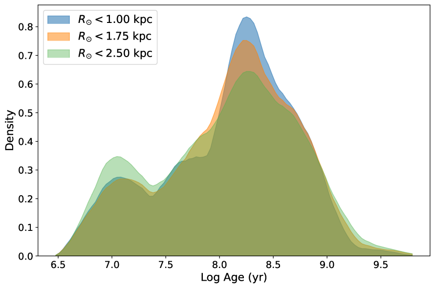
Figure 3: KDEs for the age distribution of OCs in different cylindrical cuts. The blue KDE corresponds to R = 1.00 kpc, the orange to R = 1.75 kpc and the green to R = 2.50 kpc.

2.4 Vertical Distribution

The vertical distributions of OCs for the different age groups and cylindrical cuts are represented in figure 4. The plots present, in blue, KDEs of the distribution using an exponential kernel. The uncertainties of the bins correspond to $1\sigma$ Poisson error and the widths of the bins are obtained using Knuth’s rule (Knuth 2006). The SHs were calculated analytically with its maximum likelihood estimator assuming a Laplacian (double exponential) distribution:

$$\phi(Z;\text{ }S_{H},Z_{\odot})=\frac{1}{2S_{H}}e^{-(|Z-Z_{\odot}|)/S_{H}}$$ (1)

where $Z_{\odot}$ is the median of the distribution and a measure of the Sun’s vertical displacement in relation to the GP. The SH maximum likelihood estimator can be computed analytically, being the mean absolute deviation (MAD) from the median. The values presented for the SH are the average of the 1000 bootstrap runs (Efron 1979) and the respective errors are the standard deviations. The orange lines represent the best fit a Laplacian curve.

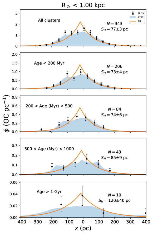
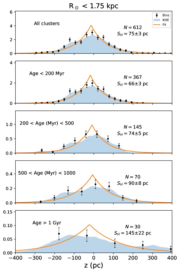
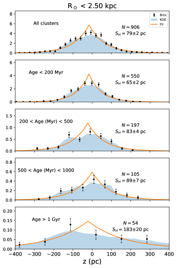
Figure 4: Vertical distribution of the OCs catalogued in (Dias et al. 2021) on the GP for different age groups and for the considered cylindrical cuts. The filled curve represents a KDE using an exponential kernel and the the solid lines are fits with the form of equation 1.

Figure 4 readily shows that all cylindrical cuts present a SH increase with age, similarly to what was reported in previous studies (such as those listed in Table 1). Nevertheless, we note that with respect to the older pre-Gaia studies, the increase of the SH with age is less accentuated; similarly to Joshi & Malhotra (2023) and in contrast to Bonatto et al. (2006), we find a large, yet finite, SH for the older OCs. This is a clear result of using a more complete catalogue with more accurate determinations of OC properties.

For the age groups with ages $<1$ Gyr, the SH evolution is consistent, within the errors, between the different cylinder cuts. This suggests that the effects of incompleteness do not impact, at least to a significant extent, the SH evolution. For the last age group, the large uncertainties make it challenging to draw any conclusions about the influence of the sample incompleteness. Nevertheless, the SH seems to increase roughly 20 pc in subsequent cylindrical cuts. It is conceivable that, whilst the decline of the completeness for the older age group is less pronounced compared to the other age groups, some missing OCs may be located closer to the GP, where their detection is more challenging. Given the relatively small sample size of the older age group, the absence of just a few OCs closer to the GP can significantly affect the estimated SH value.

Finally, it worth noticing that the OCs with ages $<200$ Myr for R${}_{\odot}<1$ kpc have a relatively high SH in comparison to the other cylindrical cuts. It is possible to notice a peak in the vertical distribution of OCs at roughly $-150<\text{z (pc)}<-100$ for the young. This corresponds to the Orion star forming region.

2.5 Sample Selection

The 2.50 kpc cut is very likely to be significantly incomplete and the 1.00 kpc cut has a very reduced number of old OCs, which leads to large uncertainties. Moreover, the impact of local structures (Orion) on the vertical distribution is evident due to the reduced number of OCs in this cut. Thus our final selection is the cylinder with a radius of 1.75 kpc, as we believe this selection finds a well-balanced compromise of the discussed trade-offs.

Furthermore, we restrict our analysis to OCs with ages up to of 2 Gyr. As detailed in section  2.3, the population of OCs older than $\sim$ 1 Gyr is notably small. Only 6 OCs are removed, constituting 20% of the old population and roughly 1% of the total number of OCs in the 1.75 kpc cut. This will substantially decrease the computational time of studying the OC population up to $\sim 10$ Gyr. The SH of the old OCs (1 Gyr $<$ age $<$ 2 Gyr) group changes from $145\pm 22$ pc to $134\pm 21$ pc and the SH of all OCs (age $<$ 2 Gyr) changes from $75\pm 3$ pc to $74\pm 2$ pc. Table 3 shows the parameters of interest for the selected cut.

Table 3: Summary table. Properties of the vertical distribution of the OC samples in the cylinder cut $R_{\odot}\leq 1.75$ kpc.

Age Group (Myr)	Sample Size	$S_{H}$ (pc)	$Z_{\odot}$ (pc)
$\leq 2000$	606	74 $\pm$ 2	14 $\pm$ 3
0 - 200	367	66 $\pm$ 3	17 $\pm$ 4
200 - 500	125	74 $\pm$ 5	9 $\pm$ 7
500 - 1000	90	90 $\pm$ 8	6 $\pm$ 6
1000 - 2000	24	134 $\pm$ 21	21 $\pm$ 26
$>$ 2000	6	–	–

3 The Model

3.1 Overview

As discussed in section 1, we propose that the apparent increase of the OC SH with age can be explained by the stronger disruption near the GP due to interactions with the GMCs. However, encounters with GMCs are not the only mechanism of disruption that the OCs are subjected throughout their lifetimes. Internal processes, such as stellar and dynamical evolution, contribute to a gradual mass loss of the OC, and to their eventual dispersion. We refer to the mass loss by dynamical evolution as the mass lost due to both evaporation and the gravitational stripping effects of the Galactic tidal field. Account for these processes is essential for reproducing the total number of OCs that survive with age. The computational model has thus the following ingredients:

1. Generation of OCs with:

   • A specified cluster formation rate (CFR).

   • Heights following a Laplace distribution.

   • Masses drawn from an initial mass distribution (Initial Cluster Mass Function - ICMF).

2. Integration of OC orbits under the Milky Way potential.

3. Disruption of OCs by different mechanisms:

   • Encounters with GMCs.

   • Mass loss due to stellar evolution.

   • Mass loss due to dynamical evolution.

The probability of the encounters depends on the vertical distance of the OCs to the GP. For simplicity, our model considers that every encounter with GMCs leads to the complete disruption of the OC. Later, possible implications of this assumption will be discussed. On the other hand, stellar and dynamical evolution will gradually decrease the mass of the OCs. When a minimum mass reached, the OC is considered disrupted. Figure 5 shows a schematic overview of the model.

In this section we will discuss the details of the model implementation. In the end of the section we present summarised overview of the model parameters. The inference of the parameters is presented in the next section.

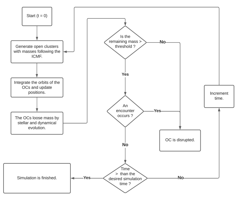
Figure 5: Flow chart of the proposed model to explain the SH evolution.

3.2 Generation of OCs

We consider the CFR to be constant and, in every increment of time, the model generates 10 OCs with different masses and orbits. Each increment of time corresponds to 0.2 Myr. We note that the number of generated clusters is arbitrary and that the resulting numbers of clusters will be later scaled to match the size of the observed sample.

3.2.1 Spatial Distribution

As discussed in section 2, the sample completeness decreases with heliocentric distance. As discussed, figure 2 shows that the ages groups younger than 1 Gyr exhibit similar declines of the surface density at all probed distances. However, we note that the age group $500<$ age (Myr) $<1000$ demonstrates a pronounced decline at closer distances (up $\sim$ 1 kpc), compared to the other age groups younger than $1000$ Myr. This is likely a fluctuation rising from the less populated inner distances, thus not differing much from the average spatial distribution of the three young age groups. Nevertheless, we have opted for a conservative approach, choosing to generate OCs following the spatial distribution of OCs with ages $<500$ Myr.

Figure 6 shows a comparison between the projected spatial distributions of observational data and an example of a randomly generated distribution. This is achieved by generating OCs uniformly in a cylinder with a radius of 1.75 kpc and then select OCs depending on their positions in the XY plane. This is made by fitting a KDE to the data and obtain the probabilities for the OCs positions. The selection of OCs is made by mapping uniform random numbers between 0 and 1 onto the normalised cumulative distribution derived from the KDE. The bandwidth of the KDE is 400 pc and it was chosen to ensure that the decline of the number of OCs with heliocentric distance is in agreement with the observed sample.

Similarly to the age groups discussed in this paper, the height distribution of OCs at birth is approximated by a Laplace distribution as given in equation 1. We will designate the height distribution of the OCs at birth as the initial cluster height function (ICHF), and the corresponding scale height as the Birth Scale Height, $B_{SH}$.

3.2.2 Initial Velocities

To integrate the OC orbits we employ the galpy Python package for galactic dynamics (Bovy 2015), as further detailed in section 3.3. The spatial coordinates are provided as $(x,y,z)$, using the galactocentric coordinate frame from astropy SkyCoord. Consequently, orbit integration with galpy requires initial values for all 3 velocity components.

Although this work is concerned with vertical motions perpendicular to the Galactic plane, OCs also revolve around the centre of the MW. Because the orbital velocity depends on the distance from the Galactic centre, it is necessary that this is correctly attributed for each OC. galpy allows to calculate the $V_{T}$ for different galactocentric distances. Thus the initial $V_{x}$ and $V_{y}$ for each OC can be easily derived from the initial $V_{T}$. In this work, we do not not consider velocity dispersions with respect to the rotation curve.

Moreover, it is important to note that OCs form with a certain V${}_{\text{z}}$. In this study, we consider that the OCs are ”dropped” in the galaxy potential, i.e, formed with V${}_{\text{z}}=0$. The implications of this assumption will be addressed later. In a future study, we aim to analyse the velocity profiles of young OCs, determine the distribution of their initial velocities, and compare to observations.

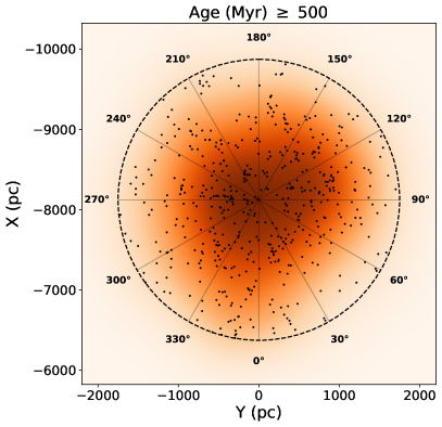
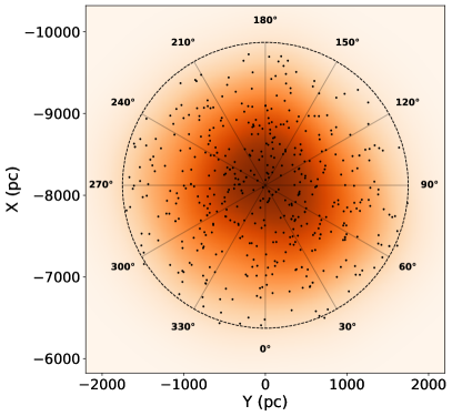
Figure 6: Left: spatial distribution of OCs projected onto the GP, for OCs ages $<500$ Myr and $R_{\odot}<1.75$ kpc. Right: example of a random generated spatial distribution of OCs. Both plots include KDEs for better comparison of the decrease of the number density with heliocentric distance.

3.2.3 Initial Cluster Mass Function

In our model the OCs are completely disrupted in every encounter and thus there is no need for an ICMF in that regard. However, we also account for additional mass loss by dynamical and stellar evolution, that are mass dependent processes (Lamers et al. 2005a). Implementing an ICMF not only makes the model more realistic, but as it also provides the means to explore in the future, the impact of OCs not being completely disrupted in single encounters with GMCs.

Following Lada & Lada (2003); Bik et al. (2003), we adopt an ICMF described by a power-law: $dN/dM\propto M^{-\alpha}\text{ with }\alpha\approx 2$ (Lada & Lada 2003; Bik et al. 2003). To generate OCs following this mass distribution, we use the inverse transform sampling method. The masses are obtained by substituting a random generated number between 0 and 1 in the following expression:

$$M=\bigg{(}\frac{1}{M_{min}}-\mu\text{ }\bigg{(}\frac{1}{M_{min}}-\frac{1}{M_{max}}\bigg{)}\bigg{)}^{-1}$$ (2)

We adopt $M_{min}=10^{2}M_{\odot}$ and $M_{max}=3\cdot 10^{4}M_{\odot}$ (as suggested by Lamers & Gieles 2006, for clusters in the solar neighborhood).

3.3 Orbit Integration

As already referred, OC orbits are integrated using galpy (Bovy 2015). We select the axisymmetric MW potential, MWPotential2014, recommended by Bovy (2015). It has 3 components: a bulge with a density profile given by a power-law with an exponential cut-off, a disc described by the Myamoto-Nagai potential (Miyamoto & Nagai 1975) and a dark matter halo modelled with a Navarro-Frenk-White potential (NFW; (Navarro et al. 1996)). We use the default values of galpy for each component (see Bovy 2015, for detailed description of the adjustment of the different components.).

By specifying the initial conditions, one can integrate the orbits for any evolution time with the desired time-steps. The orbits can be initialised using different coordinate frames, containing positional coordinates and velocity components. As already mentioned, we use the galactocentric frame from astropy SkyCoord. It is worth noting that the default values for the position of the Sun, which are used for scaling the potential, differ between galpy and astropy. To ensure consistency, as outlined in galpy documentation, one should specify in the astropy coordinate frame the following: Sun’s distance to the Galactic centre, $R_{\odot}=8$ kpc; Sun’s height, $Z_{\odot}=15$ pc and velocity components $(V_{x},V_{y},V_{z})=$ (10, 235, 7) km/s.

3.4 OC Disruption Mechanisms

Here we describe how encounters with GMCs combined with stellar and dynamical evolution are included in the model.

We start by considering that an OC is disrupted if any of the following conditions are met:

• the OC encounters a GMC.

• the OC reaches a minimum mass threshold (due to the gradual mass loss caused by stellar and dynamical evolution).

The minimum mass threshold that we define depends on the observational capacity of detecting an OC. Clusters with low masses and thus a very small number of stars are very hard to detect due to their low luminosities and density contrast with the field along the line of sight. In Piskunov et al. (2008), the authors estimate the masses of 236 OCs using the tidal radius. The minimum mass estimated was $\sim 18M_{\odot}$. Recently, Almeida et al. (2023) using Gaia early DR3 determined masses of 773 OCs within $\sim 4$ kpc from the Sun and found a minimum mass of $\sim 60M_{\odot}$. Also, our own work (Duarte Almeida et al. in prep) indicates the presence of a few stellar aggregates with masses down to $\sim 20M_{\odot}$ although almost all OCs have masses in excess of $\sim 67M_{\odot}$. Here, we will adopt the conservative value $\sim 18M_{\odot}$ for our minimum mass threshold. In any case, given the quick dispersal times of low mass clusters Lamers & Gieles (2006), adopting any of these values will not make a difference.

3.4.1 Encounters with GMCs

The implementation of this mechanism in our model has the following assumptions:

1. The vertical distribution of GMCs can be well approximated by a Laplace distribution.

2. An homogeneous distribution of GMCs around the GP.

3. Every encounter leads to the complete disruption of the OC.

Although GMCs exhibit a clumpy distribution around the GP at smaller scales ($\sim 100$ pc) (e.g. Dame et al. 2001), our model makes the simplifying approximation of an average homogeneous distribution. This should not influence the results on the kpc scales addressed in this study.

Considering the previous assumptions, the probability of an encounter is associated to the spatial distribution of the GMCs:

$$p(\text{z};\text{D}_{\text{SH}})=p_{0}\hskip 1.70709pt\text{exp}\left({-\frac{|Z|}{\text{D}_{\text{SH}}}}\right)$$ (3)

Here p₀ is interpreted as the scale factor that regulates the intensity of the disruption of OCs due to encounters with GMCs. The $D_{SH}$ stands for dissolution scale height and represents the effective SH of the disruption due to encounters. Higher values of $D_{SH}$, imply that OCs at greater distances to the GP are more affected by encounters with GMCs.

At each time step, the model assesses the probability of an encounter for each OC. Subsequently, a uniformly distributed random number between 0 and 1 is drawn and, if this number is higher than the probability of an encounter, the cluster is considered disrupted.

3.4.2 Stellar and Dynamical Evolution

In contrast to the encounters with GMCs, the disruption due to stellar and dynamical evolution is implemented as a gradual mass loss in each OC in every time-step. As shown in figure 5, in every time-step we update the masses of the OCs after loosing mass due to stellar and dynamical evolution.

In Lamers et al. (2005a) the two effects are combined in a numeric approximation given by a single expression. Hereafter we summarise the description made in Lamers et al. (2005a). For a more detailed description, we refer the reader to the original study.

Lamers et al. (2005b) show that the fraction of the initial cluster mass that is lost by stellar evolution can be approximated by a function of the form:

$$\log q_{ev}(t)=(\log t-a_{ev})^{b_{ev}}+c_{ev}\text{ for }t>12.5\text{ Myr }$$ (4)

Here $q_{ev}(t)$ is the fraction of the initial cluster mass that is lost by stellar evolution and $a_{ev}$, $b_{ev}$, $c_{ev}$ are constants (see Lamers et al. 2005b, to consult the inferred values). Notice that this function being only being for $t>12.5$ Myr is not problem because stars with lifetimes shorter than 12.5 Myr are the more massive ones, which are way less abundant and have a small contribution to the total cluster mass, making mass loss due to stellar evolution in the first 12.5 Myr negligible (Lamers et al. 2005a).

Regarding the dynamical evolution, Boutloukos & Lamers (2003) concluded that the disruption time of clusters depends on the initial mass as $t_{dis}\approx M_{i}^{\gamma}$. In the study, empirical estimation yielded $\gamma\approx 0.6$ for different local environments. Baumgardt & Makino (2003) performed N-body simulations of clusters in the tidal field of our galaxy, considering different initial masses, initial concentrations and ellipticity of orbits at different galactocentric distances. The simulations accounted for mass loss due to both stellar evolution and tidal relaxation. The study lead to the conclusion that the disruption time of clusters in the Galactic tidal field can be expressed as:

$$t_{dis}=t_{0}\left(\frac{M_{i}}{M_{\odot}}\right)^{\gamma}$$ (5)

Where $M_{i}$ is the initial mass of the cluster and $t_{0}$ is a normalisation factor that depends on the tidal field, the ellipticity of the cluster orbit and on the ambient density. Later, Lamers et al. (2005b) also studied the dependency of $t_{dis}$ with $\gamma$ for different galaxies and for the solar neighbourhood. The results also indicate $\gamma\approx 0.6$. We adopt the value used in Lamers et al. (2005a): $\gamma=0.62$

Finally, the mass loss due to both effects can be combined and approximated by:

$$\mu(t;M_{i})\equiv\frac{M(t)}{M_{i}}\approx\left[(\mu_{ev}(t))^{\gamma}-\frac{\gamma t}{t_{0}}\left(\frac{M_{\odot}}{M_{i}}\right)^{\gamma}\right]^{1/\gamma}$$ (6)

$\mu_{ev}(t)$ is the fraction of the initial mass of the cluster that would have remained at a given age, t, if the cluster is only loosing mass due to stellar evolution. Hence $\mu_{ev}(t)=1-q_{ev}(t)$. The first term describes the mass loss due to stellar evolution and the second term describes the mass loss caused by dynamical evolution. We allow $t_{0}$ to be a parameter of our model. There are two reasons that lead us not to use the value estimated in the original study:

1. Our model includes an additional contribution for the disruption of the OCs: encounters with GMCs. In Lamers et al. (2005a), the authors estimate $t_{0}$ by considering that the total mass loss in OCs is described by equation 6.

2. Lamers et al. (2005a) estimate $t_{0}$ by reproducing the age distribution of the OCs, within 600 pc from the sun, for the OC catalogue of Kharchenko et al. (2005). However, with Gaia the OC data has changed dramatically in recent years and this value may not accurately replicate the more recent observational data.

To summarise, we list below the free parameters of the model along with their descriptions:

• B${}_{\text{SH}}$ (pc) - Scale height of OCs at birth.

• $p_{0}$ - Scale factor of the probability of encounters with GMCs.

• $D_{\text{SH}}$ (pc) - Scale height for the disruptive effects of encounters with GMCs.

• $t_{0}$ (yr) - Timescale for the disruption due to dynamical evolution.

4 Parameters Inference

In this section we address the four free parameters of our model: $B_{\text{SH}}$, $p_{0}$, $D_{\text{SH}}$ and $t_{0}$. First, we explore how to adjust $B_{\text{SH}}$. Then, we address the parameters responsible for the disruption of the OCs, discussing their interrelations and influence on the SH evolution and on the number of clusters that survive at each age.

4.1 Birth Scale Height

The first parameter to consider is the birth scale height, $B_{\text{SH}}$. Ideally, it would be determined from observations of spatial distribution of clusters at birth time. However, this is hampered by several difficulties. The first one is the small numbers of newly born clusters (e.g. younger that 1 Myr) in the solar neighbourhood, which would provide poor statistics. Furthermore, most very young clusters are still deeply embedded in their parent molecular clouds (e.g Lada & Lada 2003), being only observable at infrared wavelengths, i.e. out of the reach of Gaia. Given this situation, we need to consider a somewhat older sample and take into account the evolutionary effects that might affect the inference of the $B_{\text{SH}}$, as we will do below.

To better understand what might be a good age limit to make this comparison, figure 7 shows for a $B_{\text{SH}}=92$ pc, the cumulative SH evolution of 4 runs of the model with different parameter combinations, along with the observations. This gives a first glimpse of the effects of each parameter on the OC scale height evolution. It is immediately seen that the SH grows with age for the data as well as for the simulations (except for the simulation with no disruption from GMCs, in brown and blue). Although there are small fluctuations in the modelled SH evolutions for younger ages, the SH grows systematically after 150 Myr.

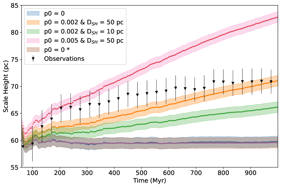
Figure 7: Comparison of the SH evolution for different combination of parameters with $B_{\text{SH}}=92$ pc and for the observations. The black triangles are the mean SH obtained from 1000 bootstrap runs on the observational sample and the error bars are the standard deviations; the blue curve corresponds to a run of the without any disruption mechanism activated; the brown curve includes only mass loss due to stellar and dynamical evolution; the pink, orange and green curves include only disruption due to encounters with GMCs, with different intensities and dissolution scale heights. The curves correspond to the averages of 10 independent runs and the shaded regions are the standard deviations.

For times $<100$ Myr, the curves overlap almost perfectly, except for the pink curve, which is slightly above. This indicates that the dissolution mechanisms here considered do not have a significant effect in that time frame. Thus, we adjust the $B_{SH}$ to match the SH of the observations considering only the OCs younger than 100 Myr. Considering the 1.75 kpc cylindrical cut, the catalogue has 228 OCs with age $<100$ Myr and a corresponding SH of $59\pm 3$ pc. This value is calculated by using 1000 bootstrap runs. Note however that the $B_{SH}$ will be necessarily larger than the observed SH. There are two reasons for this:

1. As the OCs form, the gravitational potential makes them fall towards the GP. Therefore, when we observe the population of OCs, on average, the heights will be smaller than the initial heights at which the OCs were dropped.

2. Initial $V_{z}\neq 0$, reduces this effect as the additional kinetic energy increases the vertical amplitudes of the orbits, allowing them to reach larger heights. This allows the possibility of the OCs being observed at larger heights than those at which they were formed. Because in our model the OCs are formed with the initial $V_{z}=0$, at any given time, the heights of the OCs will be necessarily equal to or smaller than their initial heights.

Using the model with no disruption activated, we find that the relation between the observed SH at 100 Myr ($O_{SH}$) and the $B_{SH}$ is linear: $O_{SH}=mB_{SH}$, with $m=0.639\pm 0.001$. As mentioned above, the SH for OCs with age $<100$ Myr is $59\pm 3$ pc. This leads to adopting a value of $B_{SH}=92\pm 5$ pc, where the uncertainty was calculated using error propagation.

We remark that the actual $B_{SH}$ of OCs may be smaller than this value, due to initial velocities as discussed, but also because we might be missing some very young OCs as their light gets blocked by the gas of the clouds in which they formed. This means that we will be missing some low altitude clusters, artificially increasing the $O_{SH}$.

4.2 Disruption parameters

With the $B_{SH}$ fixed, we can now explore how the other parameters affect the SH evolution. We start by noting that although figure 7 shows that $t_{0}$ does not affect the SH evolution of the simulations without GMC encounters, the situation changes when interactions with GMCs are considered. Despite $p_{0}$ and $D_{SH}$ being the parameters directly related with the encounters with GMCs, the study of these parameters can not be made independently of $t_{0}$. This is easily understood with an extreme example: a very strong mass loss by stellar and dynamical evolution will disrupt OCs before they have the opportunity to encounter GMCs. Thus if the OCs loose more mass due to these mechanisms (decrease of $t_{0}$), the probability of encounters has to increase, either by increasing $p_{0}$ and/or $D_{SH}$, allowing the OCs to encounter GMCs before being disrupted. The same logic applies to the opposite scenario of the OCs loosing less mass due to stellar and dynamical evolution (increase of $t_{0}$). For clarity, figure 8 shows how different values of $t_{0}$ affect the SH evolution. The different curves have the same $p_{0}$ and $D_{SH}$.

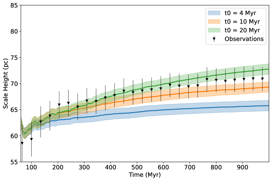
Figure 8: Comparison of the SH evolution for runs with different values of $t_{0}$ ($B_{\text{SH}}=92$ pc, $p_{0}$ = 0.004 and $D_{SH}$ = 30 pc). The curves correspond to the averages of 10 independent runs and the shaded regions are the standard deviations. The black triangles are the mean SH obtained from 1000 bootstrap runs on the observational sample and the error bars are the standard deviations

Additionally, even though $p_{0}$ and $D_{SH}$ are conceptually different, different combinations of these parameters lead to similar rates of disruption by encounters with GMCs. Thus the model displays some degeneracy in its parameters. To address this, we compare not only the SH evolution but also the total number of clusters alive at different ages. We conduct a grid search to find the best solutions, assessing their fit quality in the following way:

1. Compare the total number of OCs that are younger than a given age for the ages between 10 and 1000 Myr with a 20 Myr step. The decision to limit the comparison to ages up to 1000 Myr is motivated by the distinct trends observed in figures 1 and 2, where the numbers of OCs exhibit a distinct decrease for ages greater than 1000 Myr. Consequently, OCs were generated based on the spatial distribution of the younger population (ages $<500$ Myr) to accurately reflect the evolution of numbers, leading to the exclusion of ages older than 1000 Myr from this analysis. For a proper comparison, the number of OCs from the results needs to be scaled to the observations. To estimate the scaling factor, we apply a least squares estimation. The quality of the fit is calculated using the log-likelihood estimation. Because we are comparing cumulative distributions, where the number of OCs in each subsequent bin is dependent on the number of the previous bin, the covariance matrix needs to be included into the maximum likelihood estimation. The log-likelihood, for each independent run, is given by (James et al. 2013):

   $$l(x;\mu,\Sigma,N)=-\frac{\text{N}}{2}\ln{(2\pi)}-\frac{\text{N}}{2}\ln|\Sigma|-\frac{1}{2}(x-\mu)^{\text{T}}\Sigma^{-1}(x-\mu)$$ (7)

   where N is the total number of bins, $\Sigma$ is the covariance matrix, $\mu$ is a vector with the expected values, i.e, the observed values for each bin and $x$ is the vector with the number of OCs in each bin from the simulation. Note that $\Sigma$ will be a triangular matrix due to the nature of a cumulative distribution, i.e, subsequent bins do not affect the previous ones. Furthermore, increasing the number of OCs in an arbitrary bin by an arbitrary value, K, will increase the values of the following bins by K as well, meaning that the correlation is 1. Thus the covariance matrix is written as:

   $$\Sigma=\begin{bmatrix}\sigma(b_{1})^{2}&0&0&\cdot\cdot\cdot&0\\ \sigma(b_{2})\sigma(b_{1})&\sigma(b_{2})^{2}&0&\cdot\cdot\cdot&0\\ \sigma(b_{3})\sigma(b_{1})&\sigma(b_{3})\sigma(b_{2})&\sigma(b_{3})^{2}&\cdot\cdot\cdot&0\\ \vdots&\vdots&\vdots&\ddots&\vdots\\ \sigma(b_{n})\sigma(b_{1})&\sigma(b_{n})\sigma(b_{2})&\sigma(b_{n})\sigma(b_{3})&\cdot\cdot\cdot&\sigma(b_{n})^{2}\end{bmatrix}$$ (8)

   The values of $\sigma_{i}$ are the 1$\sigma$ Poisson errors of each bin.

2. Compare the SH evolution from the simulations and the observations in the proposed age groups. Furthermore, we also include additional age intervals to make a more robust estimation (the additional age intervals are shown in section  5.1). For the SH, we still consider OCs with ages up to 2000 Myr. Notice that their vertical distribution should be independent of the the total number of OCs. Once again, we assess the quality of the fit by calculating the log-likelihood estimation. The covariance matrix is no longer required for the SH since we do not use a cumulative distribution. Thus, the log-likelihood can be simplified:

   $$l(x;\mu,\sigma,N)=-\frac{\text{N}}{2}\ln{(2\pi)}-\sum_{i=1}^{N}\left[\frac{\text{1}}{2}\ln{|\sigma_{i}|}+\frac{(x_{i}-\mu_{i})^{2}}{2\sigma^{2}}\right]$$ (9)

   Here $\mu_{i}$ is the SH from the observations for each bin and $\sigma_{i}$ is the corresponding standard deviation. Both values are obtained from 1000 bootstrap runs. $x_{i}$ represent the average value of the SH, for 10 independent runs, in the corresponding age bin and for a specific combination of parameters.

3. The final score for the goodness-of-fit is given by the sum of both log-likelihoods: the age and numbers evolution and the SH evolution. Because the two log-likelihoods have different ranges of values, we scale each one between 0 and 1.

We present heatmaps for multiple combinations of $p_{0}$ and $D_{SH}$. Each heatmap corresponds to a specific value of $t_{0}$. Darker colours indicate a better fit to the observations. It is important to mention that the implementation of the covariance matrix in the maximum likelihood estimation was fundamental to remove, partially, the degeneracy in the parameters space. We note the usual practice in the literature is to fit cumulative distributions without considering that cumulative bins are correlated.

The values of $t_{0}$ that better fit the observations are considerably larger than the one estimated in Lamers et al. (2005a) (3.3 Myr). As discussed earlier, this was expected since their value included the (dominant) effect of encounters with GMCs. Although the heatmap for $t_{0}=10$ Myr displays good fits, we argue that $t_{0}=11$ Myr may yield even better results:

• Considering an initial $V_{z}=0$ might cause the need for smaller values of $D_{SH}$. This happens because the OCs will have smaller velocities when crossing the GP. As a result, they spend more time closer to the GP, increasing the overall probability of an encounter with a GMC. Secondly, considering $V_{z}\neq 0$ will increase the amplitude of the orbits, meaning that they will spend less time at closer distances to the GP, and thus less probability of encounters. The combination of these aspects, can possibly lead to a bias towards small values of $D_{SH}$.

• Although the SH of distribution of GMCs is known to be very small, roughly 20 pc Stark & Lee (2005), their sizes can range from a few pc to $\sim$ 200 pc (Lada & Dame 2020). While the effective SH is not catalogued, the half-thickness at half-intensity of the CO layer is found to be $\sim$ 70 pc in the solar vicinity (Malhotra 1994). Given that the $D_{SH}$ in the model represents the effective scale height of mechanism of disruption by encounters, we find that it is likely that the $D_{SH}$ is larger than the somewhat low values (30-50 pc) suggested from the fits using $t_{0}=10$ Myr.

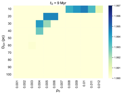
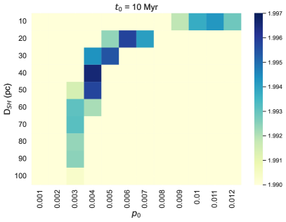
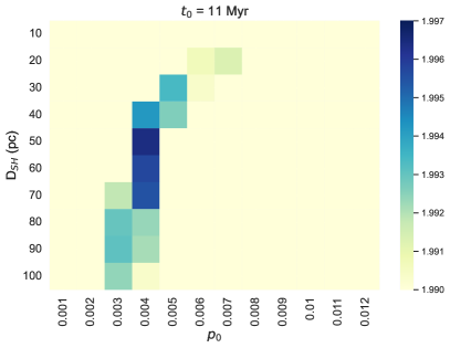
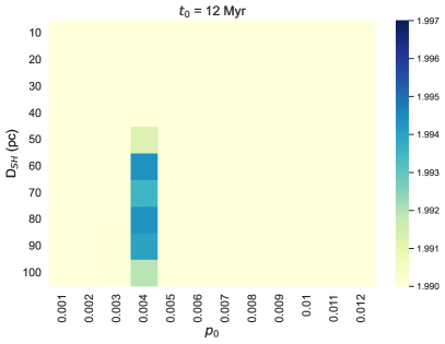
Figure 9: Heatmaps based on the combined log-likelihood estimations for different combinations of parameters.

5 Discussion

5.1 Scale Height Evolution

Figure 10 compares the SH evolution seen in the the data to the average simulation results using our adopted parameters: $B_{SH}=92$ pc, $D_{SH}=50$ pc, $p_{0}=0.004$ and $t_{0}=11$ Myr. Each bin has a width of log(age) = 0.6. The bin positions are centred, i.e, each bin contains OCs in the interval [$\text{Bin log(age)}-0.3$, $\text{Bin log(age)}+0.3$]. These are additional age groups we considered in inferring the optimal parameters. Notice that each bin includes half of the age interval of the previous one. The errors bars of the data are obtained from the standard deviations of 1000 bootstrap runs and the corresponding SH is the average of those runs. The SHs of the simulations are obtained from the average of 10 independent runs and the error bars are the corresponding standard deviations of the SH for those runs. Overall, the agreement is excellent.

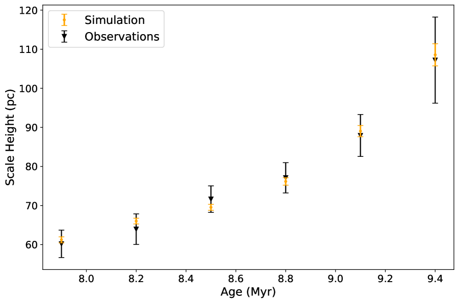
Figure 10: Comparison of the SH evolution predicted by the model (orange dots) to the observations. The model parameters used were: $B_{SH}=92$ pc, $D_{SH}=50$ pc, $p_{0}=0.004$ and $t_{0}=11$ Myr.

Following the traditional representation made in (Janes & Phelps 1994) and Bonatto et al. (2006), figure 11 compares, for several age groups, the SH output from the model to observed values. The KDEs of the simulations are made by randomly selecting N elements from the resulting sample after running the model, where N corresponds to the number of OCs from the observations in the corresponding age group. The adjustment is remarkable for ages $<1$ Gyr. For ages $>1$ Gyr, the results are still within the uncertainties of the observations.

This difference might be caused from missing some old OCs close to the GP. Detecting older OCs is more challenging due to their fainter nature, making them harder to observe, especially at lower heights where field confusion and light absorption by interstellar dust are more prominent. Notice that even though the decrease of the completeness of the older age group is less accentuated than that observed for the younger age groups (figure 2), this is a relatively small sample, with only 24 OCs. Thus, missing just a few old OCs close to the GP will significantly increase the determination of the the observed SH.

Aside from the observational difficulties, it is possible that the discrepancy for the older age group arises from the simplicity of the model. The assumption that disruption by encounters is independent of OC masses, and other intrinsic properties (e.g., radius, density, internal velocity dispersion), could potentially impact the results. Moreover, not considering initial vertical velocities affects the dynamics of the orbits of the OCs, which likely impacts the overall evolution of the SH.

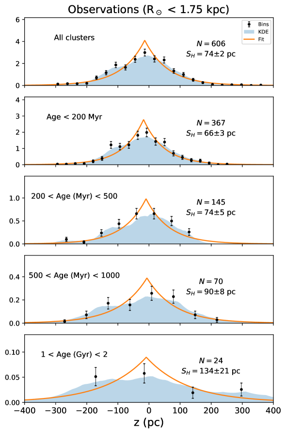
Figure 11: Comparison of the SH in the considered age groups. On the left: SH of the different age groups predicted by the model using $B_{SH}=92$ pc, $D_{SH}=50$ pc, $p_{0}=0.004$ and $t_{0}=11$ Myr. On the right: the SH of the observational data (Dias et al. 2021). The filled curve represents a KDE using an exponential kernel and the the solid lines are fits with the form of equation 1.

5.2 Age and OC number evolution

Figure 12 shows the comparison of the evolution of the total number of clusters younger than a certain age. The good agreement shows that the model can accurately reproduce not only the SH evolution but also the timescale of disruption. In older versions of the model, this was not possible because we solely considered disruption due to encounters with GMCs. It was quickly realised that, to match the total number of OCs that survive at each age, the SH evolution would have to be compromised. The necessary increase in encounter probability would lead to an overestimated SH evolution. The introduction of the ICMF and the possibility for OCs to gradually lose mass, irrespective of their heights, enabled the model to reproduce the total number of surviving OCs without compromising the SH evolution.

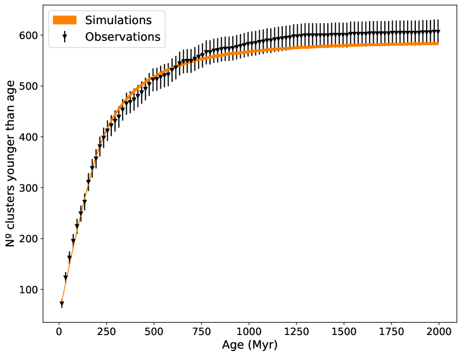
Figure 12: Comparison of the evolution of the total number of OCs younger than time using $B_{SH}=92$ pc, $D_{SH}=50$ pc, $p_{0}=0.004$ and $t_{0}=11$ Myr. The error bars of the observations correspond to 1$\sigma$ Poisson errors. The values presented for the simulations are the average number observed in the 10 independent runs and the thickness of the curve is given by the standard deviations.

Although ages $>1$ Gyr were not used for constraining the evolution of the total number of clusters, the model shows good agreement for older ages. Furthermore, it is possible to find combinations of parameters that improve the adjustment for ages $>1$ Gyr. However, as we discussed above, the origin of the difference in completeness between the older age group and the younger ones is not clear. It is interesting, however, that the model under-predicts the total number of OCs for the older ages. This is expected since the OCs are generated following the completeness trend of the younger age groups, which rapidly decay with heliocentric distance, in contrast to the older group, where this decay is much less accentuated.

It is important to note that the incompleteness of the sample can impact this adjustment. Due to the cumulative nature of the distribution, it is likely that we are progressively missing more OCs as we consider older ages, raising the possibility that total intensity of disruption is being overestimated. Thus, it possible that $t_{0}$ is higher than the one estimated from the fits using our model. Additionally, The parameters related to the encounters with GMCs might also be affected due to their indirect dependence on the overall disruption caused by stellar and dynamical evolution, as discussed previously.

6 Conclusions and Future Outlook

Table 4: Best combination of parameters and their standard deviations.

Parameter	Value	Standard Deviation
$D_{SH}$ (pc)	$53.63$	$7.60$
$p_{0}$	$0.0040$	$0.0002$
$t_{0}$ (Myr)	11	–

In this study we propose a model to explain the increase of the SH with age of the OC population. We argue that the apparent thickening of the disc seen with OCs can be largely explained as a consequence of a stronger disruption of OCs near the GP, due to interactions with the disc, namely encounters with GMCs. To test our hypothesis, we developed a computation model that forms OCs with different initial masses and follows their orbits while subjecting them to different disruption mechanisms. These mechanisms are: mass loss due to stellar and dynamical evolution; encounters with GMCs in which the probability of the encounters depends on the heights of the OCs. We compare the simulation produced with our model to the Gaia-based catalogue of OCs by (Dias et al. 2021). We find that:

• The number of observed OCs decreases with heliocentric distance, indicating that the sample is incomplete. The sample incompleteness is taken into account in our model setup.

• With optimal parameters, the model remarkably reproduces the SH evolution from the observations up to 1 Gyr. For the OCs with $1000<$ age (Myr) $<2000$, the predicted SH from the model starts to deviate from the observations. Nonetheless, it remains within the error bars of the observations. The deviation can be associated with effects of incompleteness and/or the simplicity of the model.

• The model successfully reproduces the total number of OCs that survive with age. This was achieved by generating clusters following an ICMF, as well as the implementation of disruption caused by mass loss from stellar and dynamical evolution which gradually dissolve the OCs independently of their heights.

• When using maximum likelihood estimation to adjust cumulative distributions, the covariance matrix should be properly included. In this work, it was crucial to reduce the degeneracy in the parameters space.

Although the model successfully reproduces the SH evolution and the total number of clusters that survive with age, there is still room for improvement. Future perspectives include:

• The initial velocity dispersion of the OCs impacts the $B_{SH}$, the $D_{SH}$ and the overall dynamics of the OCs. To build a more realistic model, capable of providing key insights into the kinematics of the OCs and the dynamics of the Galaxy, initial velocities must be considered. This is already possible as Gaia provides proper motions and radial velocities.

• Furthermore, the model considers that the OCs are completely disrupted in single encounters. Although this assumption might hold for OCs with small masses, it is possible that the more massive OCs survive single encounters. It can be interesting to explore how other intrinsic properties of the OCs such as the density and radius impact the results and, perhaps, fix the discrepancy of the predicted SH of OCs with ages $>1$ Gyr.

• Finally, the fluctuations of the observed SH in the first $150$ Myr (e.g. figure 8) deserve a closer look. They likely encode the structure and kinematics of the distribution of OCs at birth.