Nanoscale defects as probes of time reversal symmetry breaking

Abstract

Nanoscale defects such as Nitrogen Vacancy (NV) centers can serve as sensitive and non-invasive probes of electromagnetic fields and fluctuations from materials, which in turn can be used to characterize these systems. Here we specifically discuss how NV centers can directly probe time-reversal symmetry breaking (TRSB) phenomena in low-dimensional conductors and magnetic insulators. We argue that the relaxation rate of NV centers can vary dramatically depending on whether its magnetic dipole points towards or away from the TRSB material. This effect arises from the difference in the fluctuation spectrum of left and right-polarized magnetic fields emanating from such materials. It is perhaps most dramatic in the quantum Hall setting where the NV center may experience no additional contribution to its relaxation due to the presence of the material when initialized in a particular spin state but a large decay rate when initialized in the opposite spin state. More generally, we show that the NV center relaxation rate is sensitive to the imaginary part of the wave-vector dependent Hall conductivity of a TRSB material. We argue that this can be used to determine the Hall viscosity, which can potentially distinguish candidate fractional quantum Hall states and pairing angular momentum in TRSB chiral superconductors. We also consider Wigner crystals realized in systems with large Berry curvature and discuss how the latter may be extracted from NV center relaxometry.

I Introduction

Nanoscale defects such as Nitrogen Vacancy (NV) centers have emerged as a novel probe of magnetic and electronic correlations in materials [1, 2, 3, 4]. NV centers in particular behave as qubits with a magnetic dipole moment and intrinsic level splitting [5]. When the NV center is placed near a material, it experiences a different electromagnetic environment to what it experiences in the absence of the sample. Static fields can be mapped out by changes to the level splitting(s) of the NV center states [1] (similarly to spin resonance measurements), while magnetic fluctuations orthogonal to its intrinsic dipole axis result in relaxation of the qubit at a rate proportional to the strength of magnetic fluctuations at frequency equal to the intrinsic splitting [6, 7, 8]. These magnetic fields are ideally dominated by current and/or spin fluctuations in the probed material, and thus contain information about the conductivity or spin susceptibility of the material.

Two aspects of such defects sets them apart from traditional probes. First, they are non-invasive since they do not require the application of external fields—one can view them analogously to lab microscopes that passively gather light from a specimen of interest. Second, being atomic scale point-defects, they are sensitive to highly local material properties. For instance, as discussed in Ref. [7], these probes can be used to infer wave-vector dependent conductivity in materials, at wave-vector $q\sim 1/z_{\text{NV}}$, where $z_{\text{NV}}$ is the distance of the probe from the material. (In comparison, Nuclear Magnetic Resonance which is based on similar principles, naturally probes magnetic fluctuations at wave-vectors related to the crystal structure [9].) This make these probes significant from the perspective of detecting novel correlations in materials where usual conductance or global spin-susceptibility measurements may not implicate new phenomena, or where multiple orders coexist and external fields can influence the state making measurements challenging to interpret.

NV centers have been used to map out local spin patterns [10, 11, 12], measure spin wave spectra in low dimensional magnets [13, 14], transport characteristsics (ballistic/diffusive/hydrodynamic/superconducting) of electrons [6, 15, 16, 17, 18, 19, 20], measure phononic Cherenkov effect in photoexcited graphene [21], among others. Immense progress has been made in engineering their intrinsic relaxation properties [22] to obtain $T_{1}$ times of the order of seconds at cryogenic temperatures [23], attaching them on maneuverable tips [24, 25] and controlled implantation at various depths and in ensemble [26, 27, 28, 29]. Other nanoscale defects such as silicon vacancy centers [30] among others [31] are also potential candidates for novel quantum sensing capabilities [32]. Theoretically, proposals have been made to use NV centers to measure hydrodynamic transport and Kondo impurities in metals [7], crystallization at low densities in electron gases [33], spinon Fermi surfaces in spin liquid candidates [34], and novel edge states in topological materials [35], among others [36].

In this work, we focus on how such probes can be used to ascertain time reversal symmetry breaking (TRSB) phenomena in materials of various kinds, in quantum Hall insulators, TRSB superconductors, Wigner crystals in systems exhibiting anaomlous quantum Hall phenomena, and low dimensional magnets. A key insight as to the utility of these probes comes from a simple observation—TRSB materials exhibit a circular dichroism in the electromagnetic fluctuation spectrum near them. Specifically, the spectrum of left and right circularly polarized magnetic fields is different near a TRSB material. This dichroism stems directly from the spectra of ‘circularly polarized’ current and spin operators $j_{\pm}=j_{x}\pm ij_{y},s_{\pm}=s_{x}\pm is_{y}$ (defined analogously as in electromagnetism) that are inherently different in a TRSB material. The most stark examples of this physics is the quantum Hall insulator or a quantum ferromagnet—operators $j_{+}(s_{+})$ can be used to raise Landau level index (create a magnon) from the ground state, while operators $j_{-}(s_{-})$ reduces the Landau level index (destroys a magnon) [37, 38]. At low temperatures, the spectrum of these raising and lowering operators is thus significantly different from one another, and this translates to dichroism in magnetic fluctuations near the material.

In Sec. II, we elaborate further on this dichroism, computing the $1/T^{\hat{z}}_{1},1/T^{-\hat{z}}_{1}$ relaxation rates of a magnetic dipole probe that is oriented either perpendicular, in the $\hat{z}$ direction, or anti-perpendicular, in the $-\hat{z}$ direction, to the surface of the material of interest. Note that for NV center based imagining, these are realized with a single NV center with its magnetic dipole oriented along the $\hat{z}$ axis, and measuring its relaxation to equilibrium starting from either the $\left|m_{s}=1\right>$ or $\left|m_{s}=-1\right>$ states. In the first case, the relaxation rate amounts to a sum of spectral weights $\left|b_{+}(\omega_{\text{NV}})\right|^{2}+\left|b_{-}(-\omega_{\text{NV}})\right|^{2}$, while in the second case, one probes $\left|b_{+}(-\omega_{\text{NV}})\right|^{2}+\left|b_{-}(\omega_{\text{NV}})\right|^{2}$, with $\omega_{\text{NV}}$ being the transition frequency of the NV center or more generally, the local magnetic dipole probe in use. As we show, the two components in these rates are related by detailed balance as one would expect of emission and absorption rates due to fluctuations in a thermally equilibrated system. However, these two rates consist of a contribution $\text{Im}\left[N_{xy}\right]$ (a symmetrized correlator of magnetic field fluctuations in the $x,y$ directions) that is odd under time-reversal. This piece is precisely isolated by considering the difference of the two relaxation rates, $1/T^{\hat{z}}_{1}-1/T^{-\hat{z}}_{1}$, and which directly implicates TRSB if it is non-zero.

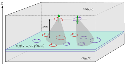
Figure 1: Magnetic noise from a time-reversal symmetry breaking sample (blue) exhibits a different spectrum for magnetic fluctuations with opposite chiralities (purple and red). The NV center is assumed to be embedded here in a dielectric of constant $\epsilon_{0}$. We assume for simplicity that the sample sits sandwiched between two dielectrics of similar dielectric constant. NV centers with magnetic dipoles (green arrows) oriented towards or against such a material exhibit different relaxation rates owing to this difference. (Note these are not implied to be two separate NV centers but the same color center initialized in the state $\left|m_{s}=\pm 1\right>$. They are shown separately here for clarity.) In particular, $\Gamma^{\pm\hat{z}}_{\text{ems}}\propto\text{Re}\left[\sigma_{T}\mp i\sigma_{H}\right](q\sim 1/z_{\text{NV}},\omega=\omega_{\text{NV}}$; see main text for details.

In Sec. III, we make a connection between $\text{Im}\left[N_{xy}\right]$, and $\text{Im}\left[\sigma_{H}(q,\omega)\right]$, that is, the imaginary part of the Hall conductivity at finite wave-vectors in the material. In particular, we study the electromagnetic fluctuation spectrum near a two dimensional TRSB material sandwiched between dielectrics. Following the standard analysis of electromagnetic waves reflecting off of conducting surfaces [39], we compute the magnetic response of the system in the presence of an added magnetic dipole, which generates both $s-$ and $p-$ polarized waves. We find that the susceptibility of interest, $\chi_{xy}$ depends only on reflections that convert $s-$ polarized light to $p-$ polarized light and vice versa, an effect fully absent in systems with time-reversal symmetry. We use the fluctuation dissipation theorem to arrive at our final result for $\text{Im}\left[N_{xy}\right]$. We find that much like the usual time-reversal preserving case, the magnetic dipole probes magnetic fluctuations at a wavevector $q\sim 1/z_{\text{NV}}$. We find that relaxation rates $1/T_{1}^{\pm\hat{z}}$ are sensitive probes of $\text{Re}\left[\sigma_{T}\mp i\sigma_{H}\right](q\sim 1/z_{\text{NV}},\omega_{\text{NV}})$, where $\sigma_{T}$ is the optical conductivity associated with current fluctuations orthogonal to $\bm{q}$.

In Sec. IV, we highlight how the two rates $1/T^{\pm\hat{z}}_{1}$ are sharply different from each other when the sample being sensed is a Hall system. The difference becomes more acute in the quantum limit with one of the two relaxation rates approaching zero. In other words, when an NV center dipole is anti-aligned with the applied magnetic field engendering the quantum Hall system, the NV center’s relaxation rate is almost exclusively determined by vacuum fluctuations present even in the absence of the Hall system. We then turn our attention to making a connection with the imaginary part of the Hall conductivity at $\mathcal{O}\left(q\ell\right)^{2}$, where $\ell$ is the magnetic length, and the Hall viscosity. The Hall viscosity is a novel term in the viscosity tensor of a two dimensional fluid breaking time reversal symmetry [40, 41, 42]. It is quantized in a quantum Hall system and related to the Wen-Zee shift [41, 43, 44]. It has been proposed that the Hall viscosity can be measured using spatially varying fields as it appears at $\mathcal{O}\left(q\ell\right)^{2}$ in the real part of the Hall conductivity, alongside another, non-topological contribution [45]. Here we compute the imaginary part of the Hall conductivity for a non-interacting integer quantum Hall system and show that the above two contributions appear as coefficients of different poles (at $\omega=\omega_{c},2\omega_{c}$), and thus the Hall viscosity may be more directly inferred from the imaginary part of the Hall conductivity, which the relaxation dynamics of the probe have access to.

In Sec. V, we consider TRSB superconductors, and note that for the chiral superconductors (using results from Refs. [46]), $\text{Im}\left[\sigma_{xy}\right]$ at $\mathcal{O}\left(qv_{F}/\Delta\right)$ contains a Hebel-Slichter like peak at $\omega=2\Delta$, where $\Delta$ is the superconducting gap. In case of a chiral superconductor, and assuming the angular momentum of the Cooper pairs is aligned with the axis of the probe dipole, this peak is proportional to the pairing channel $l$ (including its sign), and thus, whether one obtains a repression or enhancement of such a peak in the relaxation rate of the probe depends directly on the orientation of this dipole vis-a-vis the pairing angular momentum of the Cooper pairs in the TRSB superconductor. This result is also understood to arrive by noting that the Hall viscosity is given by the density of electrons times the net average angular momentum (spin and orbital) carried per electron [43, 42], and appears analogously in the imaginary part of the Hall conductivity of a chiral superconductor as in the quantum Hall system at $\mathcal{O}(q^{2})$.

In Sec. VI, we discuss how such probes may be used to infer the Berry curvature directly in some instances. Specifically, we consider the possibility of Wigner crystals in materials with Berry curvature where electrons are localized in a triangular lattice but are spinning with finite orbital angular momentum at their respective lattice sites. Specifically, as in Ref. [47], we consider the example of Bernal stacked bilayer graphene—the analysis there suggests such a Wigner crystal(WC) phase could be realized at very low densities, and the spectrum of local excitations is determined by the Berry curvature at the momentum corresponding to the minima in the free electron dispersion. This spectrum is more readily probed by an NV center probe, as we show, instead of a scanning tunneling probe where electronic interaction effects are expected to significantly alter spectral features in a localized system. Thus, one can gain information about the Berry curvature in occupied bands at momenta which can be tuned by altering the interalyer displacement field.

In Sec. VII we briefly discuss the magnetic noise from magnetic insulators, and focus on the case of a ferromagnet in particular. Much like the quantum Hall case where current $j_{\pm}$ operators have very different spectral functions at low temperatures, the spin $s_{\pm}$ operators have very different spectral functions. We find that although the relaxation rate is more suppressed for one orientation of the dipole probe versus the other, it is never as dramatic as in the quantum Hall case. This occurs due to the fact that the magnetic dipole field Kernel allows for magnetic fluctions $b_{\mp}$ to be generated by spin fluctuations of the opposite chirality $s_{\pm}$. In this sense, the quantum Hall insulators provides one of the most striking examples of TRSB using such probes. We summarize our findings in Sec. VIII.

II Chirality of magnetic fluctuations above a time-reversal symmetry breaking material

A standard probe of measuring time-reversal symmetry breaking in materials is the Polar Kerr (and related Faraday) effect [48]. When linearly polarized light is normally incident on a material which exhibits magnetization or other forms of time-reversal symmetry breaking (TRSB) phenomena, the polarization of the reflected and transmitted light is generally offset by an angle that depends on the strength of TRSB in the material. One way to rationalize this is that the phase acquired upon reflection of circularly polarized light from a TRSB material is generically different for right and left circularly polarized components. This phase lag difference, which probes the magnetization of the material, or off-diagonal components of the dielectric and conductivity tensors is the cause of the rotation of the polarization [49].

Likewise, the amplitude of the reflection and transmission coefficients are also generically different for the different circular polarizations of light. In particular, in ambient conditions, even in the absence of a probe light pulse, we can thus expect the amplitude of fluctuations of chiral components of the magnetic field to have different spectral properties, which could be detected by a suitable magnetic probe. Let us consider, for specificity, the example of an NV center which serves as an effective qubit with a magnetic moment $\mu_{\text{NV}}$ oriented perpendicular to the surface of a TRSB material. The NV center behaves as an effective spin$-1$ defect that has a static splitting $\omega_{\text{NV}}\approx 2\pi\cdot 3\text{GHz}$ between $\left|m_{s}=0\right>$ and $\left|m_{s}=\pm 1\right>$ levels in the absence of any external field (see Ref. [2] and references therein). For the purposes of sensing magnetic fields which lead to transitions with $\Delta m_{s}=\pm 1$, we can assume that the NV center is initialized either in the state $\left|m_{s}=+1\right>$ or in $\left|m_{s}=-1\right>$, with the dipole oriented along the $\hat{z}$ axis, and obtain the $1/T_{1}$ relaxation rate by considering the decay to the $\left|m_{s}=0\right>$ state (using fluorescence measurements). The relevant levels, the initialized state $\left|m_{s}=\pm 1\right>$, and the state $\left|m_{s}=0\right>$ can be described by a two level system Hamiltonian

$$H^{\pm\hat{z}}_{\text{NV}} =\pm\frac{\omega_{\text{NV}}}{2}\sigma_{z}-\bm{b}(t)\cdot\bm{\sigma}$$

$$=\pm\frac{\omega_{\text{NV}}}{2}\sigma_{z}-b_{+}(t)\sigma_{-}-b_{-}(t)\sigma_{+}-b_{z}(t)\sigma_{z},$$ (1)

where $b_{\pm}=\frac{b_{x}(t)\pm ib_{y}(t)}{2}$ are the chiral components of the external magnetic field at the NV center, $\sigma_{\pm}=\sigma_{x}\pm i\sigma_{y}$, and the $\pm\hat{z}$ signs effectively impose the choice of the initial state $\left|m_{s}=\pm 1\right>$—the state $\left|m_{s}=0\right>$ is associated with $\sigma_{z}=\mp 1$, that is, always the lower energy state, and relaxation into the $\left|m_{s}=0\right>$ state from $\left|m_{s}=\pm 1\right>$ is governed by either $b_{+}\sigma_{-}$ (+; emitting a photon with $+1$ unit of angular momentum in the $\hat{z}$ direction), or $b_{-}\sigma_{+}$ (-; emitting a photon with $-1$ unit of angular momentum in the $\hat{z}$ direction) term accordingly. Note that for clarity we have suppressed factors of $\hbar$ and the magnetic moment of the probe and associated $g$-factor. We can compute the relaxation rate $1/T_{1}=\Gamma_{\text{abs}}+\Gamma_{\text{ems}}$ of the NV center as the sum of the absorption and emission rates which in turn are given by Fermi’s Golden rule

$$\Gamma^{\hat{z}}_{\text{ems}} =2\pi\sum_{n,m}\rho_{n}\left|\left<m\vphantom{b_{+}n}\right|b_{+}\left|n\vphantom{mb_{+}}\right>\right|^{2}\delta(\omega_{\text{NV}}-\omega_{mn})$$

$$=\frac{\pi}{2}\sum_{n,m}\rho_{n}\left[\left|\left<m\vphantom{b_{x}n}\right|b_{x}\left|n\vphantom{mb_{x}}\right>\right|^{2}+\left|\left<m\vphantom{b_{y}n}\right|b_{y}\left|n\vphantom{mb_{y}}\right>\right|^{2}+2\text{Im}\left(\left<n\vphantom{b_{y}m}\right|b_{y}\left|m\vphantom{nb_{y}}\right>\left<m\vphantom{b_{x}n}\right|b_{x}\left|n\vphantom{mb_{x}}\right>\right)\right]\delta(\omega_{\text{NV}}-\omega_{mn})$$

$$\Gamma^{\hat{z}}_{\text{abs}} =2\pi\sum_{n,m}\rho_{n}\left|\left<m\vphantom{b_{-}n}\right|b_{-}\left|n\vphantom{mb_{-}}\right>\right|^{2}\delta(\omega_{\text{NV}}+\omega_{mn})$$

$$=\frac{\pi}{2}\sum_{n,m}\rho_{n}\left[\left|\left<m\vphantom{b_{x}n}\right|b_{x}\left|n\vphantom{mb_{x}}\right>\right|^{2}+\left|\left<m\vphantom{b_{y}n}\right|b_{y}\left|n\vphantom{mb_{y}}\right>\right|^{2}-2\text{Im}\left(\left<n\vphantom{b_{y}m}\right|b_{y}\left|m\vphantom{nb_{y}}\right>\left<m\vphantom{b_{x}n}\right|b_{x}\left|n\vphantom{mb_{x}}\right>\right)\right]\delta(\omega_{\text{NV}}+\omega_{mn})$$

Here $\left|n\right>,\left|m\right>$ denote many-body eigenstates of the material, with $\hbar\omega_{n},\hbar\omega_{m}$ their respective energies, $\omega_{mn}=\omega_{m}-\omega_{n}$ is the difference of energies modulo $\hbar$, and $\rho_{n}$ is the probability of the system being in state $\left|n\right>$. For convenience, we set $\hbar=1$ in what follows. Note that we make no mention of the precise kernel that connects the magnetic field to the currents/spins in the material for now, except noting that under time-reversal, these fields will flip sign, as would the current or magnetic moments generating them. It is also important to note the sign difference in the two expressions—while $\Gamma^{\hat{z}}_{\text{ems}}$ corresponds to the spectral weight of fluctuations of $b_{+}$ at frequency $\omega=\omega_{\text{NV}}$, $\Gamma^{\hat{z}}_{\text{abs}}$ relates to the spectral weight at $\omega=-\omega_{\text{NV}}$ of fluctuations of $b_{-}$.

As seen in Eq. (LABEL:eq:chiralrelaxation), the relaxation rates contain two types of terms, ones which involve magnetic fields in the same direction $\sim b_{x}^{2},b_{y}^{2}$, and another set of terms comprising both the $x$ and $y$ components of the field. The latter amount to zero in a time-reversal preserving system—we can see this by noting that the matrix elements of the magnetic field for time reversed state transform as [50]

$$\left<n\vphantom{b_{x}m}\right|b_{x}\left|m\vphantom{nb_{x}}\right>\overset{\mathcal{T}}{\rightarrow}\left<\tilde{n}\vphantom{b_{x}\tilde{m}}\right|b_{x}\left|\tilde{m}\vphantom{\tilde{n}b_{x}}\right>=\left<n\vphantom{\mathcal{T}b_{x}\mathcal{T}^{-1}m}\right|\mathcal{T}b_{x}\mathcal{T}^{-1}\left|m\vphantom{n\mathcal{T}b_{x}\mathcal{T}^{-1}}\right>^{*}=-\left<n\vphantom{b_{x}m}\right|b_{x}\left|m\vphantom{nb_{x}}\right>^{*}$$ (3)

Thus, for time-reversed states $\left|\tilde{n}\right>,\left|\tilde{m}\right>$ the second term $\sim b_{x}b_{y}$ changes sign as a result of complex conjugation. If the system has time-reversal symmetry, these states have the same energy as $\left|n\right>,\left|m\right>$ (possibly being identical to the original states), and these cross terms thus vanish. However, for a system that breaks TRSB, these terms will not in general vanish. One simple way of seeing this is to note that for a Hall system, these terms would be connected to $j_{x}-j_{y}$ current-current correlators which are linked to the presence of a finite Hall conductivity.

By itself, the presence of these TRSB terms does not provide a clear indication of TRSB in the material, because they can in principle get swamped by the terms causing NV center relaxation even in the absence of TRSB. Moreover, while it may appear tempting to define a conclusive TRSB sensing metric by subtracting the absorption rate from the emission rate because of the sign difference in the TRSB terms, we note that, assuming the material and its ambient electromagnetic environment are in thermal equilibrium, these two rates are in fact trivially related by detailed balance [51]. We can see this simply by interchanging $m\leftrightarrow n$ in $\Gamma^{\hat{z}}_{\text{abs}}$ to recover the result that $\Gamma^{\hat{z}}_{\text{abs}}=e^{-\beta\omega_{\text{NV}}}\Gamma^{\hat{z}}_{\text{ems}}$, as expected. In particular, $\Gamma^{\hat{z}}_{\text{abs}}\propto S_{-}(-\omega_{\text{NV}})$ while $\Gamma^{\hat{z}}_{\text{ems}}\propto S_{+}(\omega_{\text{NV}})$, where $S_{+},S_{-}$ are the usual spectral functions associated with $b_{+},b_{-}$ fields at the site of the NV center. Thus, for a system with TRSB, while the spectral functions for different chiralities of magnetic field fluctations can be different at the same frequency, they are nevertheless related by detailed balance at opposite ($\omega\rightarrow-\omega$) frequencies.

To directly probe TRSB, thus, we envision measuring the difference of relaxation rates from the $\left|m_{s}=+1\right>$ state (given by $\Gamma^{\hat{z}})$ and $\left|m_{s}=-1\right>$ state (given by $\Gamma^{-\hat{z}}$. Note that for relaxation from $\left|m_{s}=-1\right>$, $\Gamma^{-\hat{z}}_{\text{abs}}\propto S_{+}(-\omega_{NV})$ while $\Gamma^{-\hat{z}}_{\text{ems}}\propto S_{-}(\omega_{\text{NV}})$. The difference of these two relaxation rates can only be non-zero provided the system breaks TRSB. (More generally, say for a spin-$1/2$ point defect, one may need to have two such defects, with one whose dipole points towards the system, and another whose dipole points away from the system.) Combined with the fact that the nanoscale probes are effectively point defects whose distance from the surface of the material can be controlled (for instance, by appropriate implantation depth in diamond vis-a-vis the material surface, or by mounting the probe on a cantilever), such probes can give information about the peculiar local (wave-vector dependent) scaling of correlations associated with TRSB in the material. As we show in following sections, such a diagnostic is directly sensitive to the imgainary or dissipative part of the Hall conductivity at wave-vector $q\sim 1/z_{\text{NV}}$, where $z_{\text{NV}}$ is the distance of the probe from the material surface.

To complete this discussion, it is useful to define symmetrized and anti-symmetrized spectral functions and related susceptibilities. Specifically, we introduce

$$N_{xx(yy)}(\omega>0) =\pi\sum_{n,m}\rho_{n}\left|\left<m\vphantom{b_{x(y)}n}\right|b_{x(y)}\left|n\vphantom{mb_{x(y)}}\right>\right|^{2}\left[\delta(\omega-\omega_{mn})+\delta(\omega+\omega_{mn})\right]$$

$$N_{yx}(\omega>0) =\pi\sum_{n,m}\rho_{n}\left<n\vphantom{b_{y}m}\right|b_{y}\left|m\vphantom{nb_{y}}\right>\left<m\vphantom{b_{x}n}\right|b_{x}\left|n\vphantom{mb_{x}}\right>\left[\delta(\omega-\omega_{mn})-\delta(\omega+\omega_{mn})\right]$$

$$A_{xx}(\omega>0) =\pi\sum_{n,m}\rho_{n}\left|\left<m\vphantom{b_{x}n}\right|b_{x}\left|n\vphantom{mb_{x}}\right>\right|^{2}\left[\delta(\omega-\omega_{mn})-\delta(\omega+\omega_{mn})\right]$$

$$A_{yx}(\omega>0) =\pi\sum_{n,m}\rho_{n}\left<n\vphantom{b_{y}m}\right|b_{y}\left|m\vphantom{nb_{y}}\right>\left<m\vphantom{b_{x}n}\right|b_{x}\left|n\vphantom{mb_{x}}\right>\left[\delta(\omega-\omega_{mn})+\delta(\omega+\omega_{mn})\right]$$

where we note that

$$\frac{1}{T^{\hat{z}}_{1}} =\frac{1}{2}N_{xx}(\omega_{\text{NV}})+\frac{1}{2}N_{yy}(\omega_{\text{NV}})+\text{Im}[N_{yx}(\omega_{\text{NV}})]$$

$$\frac{1}{T^{\hat{z}}_{1}} =\coth\left(\frac{\beta\omega}{2}\right)\left[A_{xx}(\omega_{\text{NV}})+\text{Im}[A_{yx}(\omega_{\text{NV}})]\right]$$

$$\frac{1}{T^{\hat{z}}_{1}} -\frac{1}{T^{-\hat{z}}_{1}}=2\coth\frac{\beta\omega}{2}\text{Im}\left[A_{yx}(\omega_{\text{NV}})\right]$$ (4)

where we have assumed that the system respects rotational invariance and thus $A_{xx}(\omega)=A_{yy}(\omega)$. Note that $N_{xy}$ is only non-zero due to time-reversal symmetry breaking. Concurrently, we define the susceptibility

$$\chi_{b_{y(x)},b_{x}} =\mathcal{F}\left[-i\theta(t)\left<\left[b_{y(x)}(t),b_{x}(0)\right]_{-}\right>\right]$$

$$=-\sum_{n,m}\rho_{n}\bigg{[}\frac{\left<n\vphantom{b_{y(x)}m}\right|b_{y(x)}\left|m\vphantom{nb_{y(x)}}\right>\left<m\vphantom{b_{x}n}\right|b_{x}\left|n\vphantom{mb_{x}}\right>}{\omega-\omega_{\text{mn}}+i0^{+}}$$

$$\hskip 72.26999pt-\frac{\left<n\vphantom{b_{x}m}\right|b_{x}\left|m\vphantom{nb_{x}}\right>\left<m\vphantom{b_{y(x)}n}\right|b_{y(x)}\left|n\vphantom{mb_{y(x)}}\right>}{\omega+\omega_{\text{mn}}+i0^{+}}\bigg{]}.$$ (5)

which is related to the anti-symmetric correlator $A_{y(x)x}(\omega)$ by the relation $\text{Re}\left[\chi_{b_{y(x)},b_{x}}(\omega)\right]=\text{Im}\left[A_{y(x)x}(\omega)\right]$. Here we note that one may be concerned that there are contributions to $\text{Re}\left[\chi_{b_{y},b_{x}}\right]$ from terms proportional to $\text{Re}\left[\left<n\vphantom{b_{y}m}\right|b_{y}\left|m\vphantom{nb_{y}}\right>\left<m\vphantom{b_{x}n}\right|b_{x}\left|n\vphantom{mb_{x}}\right>\right]\mathcal{P}\left(\frac{1}{\omega\pm\omega_{mn}}\right)$. There are two reasons for excluding such contributions—i) these should be much smaller than the terms proportional to $\delta(\omega-\omega_{mn})$ corresponding to $\text{Im}\left[A_{yx}\right]$, and ii) in the case of the system possessing rotational symmetry, they vanish exactly since $\chi_{b_{y},b_{x}}=-\chi_{b_{x},b_{y}}$ while these terms are symmetric under the exchange $b_{x}\leftrightarrow b_{y}$. The latter can be easily intuited by noting that $\chi_{b_{y},b_{x}}$ corresponds to the magnetic field $b_{y}$ in response to a magnetic moment placed at the site of the probe with moment in the $x$ direction, and considering a $\pi/2$ rotation.

We also note that an analogous measurement of $\text{Im}[N_{yz}]$ or $\text{Im}[N_{xz}]$ is possible by orienting the dipole moment accordingly but here we focus for simplicity exclusively on $\text{Im}[N_{xy}]$.

III Measurement of chirality in conducting materials

We now evaluate $\text{Im}\left[N_{yx}(\omega)\right]$ by solving the problem of reflection of light from a two-dimensional metallic surface sandwiched between two dielectrics with the same dielectric constant $\epsilon$; see Fig. 1 for the setup. We follow the methods of Ref. [7], but allow for the two dimensional material to exhibit a Hall response owing to TRSB. To evaluate $\text{Im}\left[N_{yx}(\omega)\right]$, we first compute the susceptibility $\chi_{b_{y},b_{x}}(\bm{r})=B^{\text{total}}_{y}(\bm{r})/M_{x}(\bm{r})$ by computing the electromagnetic field set up by a local magnetic dipole at site of the probe $\bm{r}$ in the presence of the material which breaks TRSB.

To simplify this task, we use the translation symmetry along the surface of the material and calculate the magnetic field profile due to a sheet of magnetization, with an in-plane magnetic moment. Specifically, we solve for the magnetic field in the presence of a sheet of magnetization $\bm{M}=m_{0}(\hat{z}\times\hat{Q})\delta(z-z_{NV})e^{i\bm{Q}\cdot\bm{\rho}}$ and, separately, in the presence of a sheet of magnetization with $\bm{M}=m_{0}\hat{Q}\delta(z-z_{NV})e^{i\bm{Q}\cdot\bm{\rho}}$. We note that the total magnetic field due to the point dipole moment can then be found by integrating the magnetic field found (in the $y$-direction) in these two separate calculations with the Fourier factor $e^{-i\bm{Q}\cdot\bm{\rho}_{NV}}$ and using appropriate projection to $\hat{x}$, $\hat{y}$ axes. The decomposition into moments parallel to $(\hat{z}\times\hat{Q})$ and $\hat{Q}$ is done because magnetization sheets in these directions yield exclusively $p-$ and $s-$ polarized waves, respectively. In the case of systems that do not break TRSB, it is known that the reflected waves continue to retain their polarization; see Ref. [7] for the related calculation in the absence of TRSB. However, in this case, as we show, the presence of a Hall conductivity generates waves of opposite polarization as well.

III.0.1 s-polarized incident waves solution

The electric field is in-plane and the magnetic field can be found using Faraday’s Law, $\bm{B}={\nabla}\times\bm{E}/(i\omega)$,

$$\bm{E}_{in} =E_{0}\left(\hat{z}\times\hat{Q}\right)e^{i\bm{Q}\cdot\bm{\rho}-iq_{z}z},$$

$$\bm{E}_{r} =E_{0}\left[r_{ss}\left(\hat{z}\times\hat{Q}\right)+r_{sp}(-\bar{q}_{z}\hat{Q}+\bar{Q}\hat{z})\right]e^{i\bm{Q}\cdot\bm{\rho}+iq_{z}z},$$

$$\bm{E}_{t} =E_{0}\left[t_{sp}(\bar{q}_{z}\hat{Q}+\bar{Q}\hat{z})+t_{ss}\left(\hat{z}\times\hat{Q}\right)\right]e^{i\bm{Q}\cdot\bm{\rho}-iq_{z}z}.$$

$$\bm{B}_{in} =\frac{E_{0}}{\bar{c}}\left(\bar{q}_{z}\hat{Q}+\bar{Q}\hat{z}\right)e^{i\bm{Q}\cdot\bm{\rho}-iq_{z}z},$$

$$\bm{B}_{r} =\frac{E_{0}}{\bar{c}}\left[r_{ss}\left(-\bar{q}\hat{Q}+\bar{Q}\hat{z}\right)-r_{sp}(\hat{z}\times\hat{Q})\right]e^{i\bm{Q}\cdot\bm{\rho}+iq_{z}z},$$

$$\bm{B}_{t} =\frac{E_{0}}{\bar{c}}\left[t_{ss}\left(\bar{q}_{z}\hat{Q}+\bar{Q}\hat{z}\right)-t_{sp}(\hat{z}\times\hat{Q})\right]e^{i\bm{Q}\cdot\bm{\rho}-iq_{z}z}.$$

where $q_{z}=\sqrt{\epsilon\frac{\omega^{2}}{c^{2}}-Q^{2}}$, and we have defined $\bar{c}=c/\sqrt{\epsilon}$ as the speed of light in the dielectric, and a dimensionless wavevector $\bar{q}_{z}=q_{z}\bar{c}/\omega$. Thus, $\bar{q}_{z}^{2}+\bar{Q}^{2}=1$. The coefficients $r_{ss},r_{sp},t_{ss},t_{sp}$ are reflection and transmission coefficients for the case of when $s$-polarized light impinges on the sample.

To solve for the reflection and transmission coefficients, we apply the following boundary conditions: the fields $B_{z}$ and $\epsilon\bm{E}_{\parallel}$ are continuous across the interface, while the parallel component of $\bm{B}$ and $E_{z}$ are discontinuous due to the free charge and current generated at the interface, that is, $\mu_{0}\bm{J}=\hat{z}\times\left(\bm{B}_{\parallel}(0^{+})-\bm{B}_{\parallel}(0^{-})\right)$, and $\rho/\epsilon_{0}=\epsilon E_{z}(0^{+})-\epsilon E_{z}(0^{-})$. The material imposes a constraint between the charge accumulated and the longitudinal current via the continuity relation, while the current itself is given by the conductivity tensor of the material; specifically, $\bm{J}=\sigma_{L}\bm{E}_{\parallel,\hat{Q}}+\sigma_{T}\bm{E}_{\parallel,(\hat{z}\times\hat{Q})}-\sigma_{H}(\hat{z}\times\bm{E}_{\parallel})$. Note in particular the sign of $\sigma_{H}$ is determined by the definition $J_{x}=\sigma_{H}E_{y}$. Here we make a distinction between current response that is parallel or perpendicular to the modulation wave-vector $\bm{Q}$ denoting these by $\sigma_{L}$ and $\sigma_{T}$ respectively.

Putting the above together, and defining dimensionless conductivities $\bar{\sigma}_{H/L/T}=\sigma_{H/L/T}/\left(\bar{c}\epsilon_{0}\epsilon\right)$, we obtain the following consistency conditions on the reflection and trasmission coefficients:

$$1+r_{ss} =t_{ss},\;\;r_{sp}=-t_{sp},$$

$$t_{sp}\bar{\sigma}_{L}\bar{q}_{z}+t_{ss}\bar{\sigma}_{H} =r_{sp}-t_{sp},$$

$$t_{ss}\left(\bar{\sigma}_{T}+\bar{q}_{z}\right) =\bar{q}_{z}(1-r_{ss})+\bar{\sigma}_{H}\bar{q}_{z}t_{sp}.$$ (7)

Solving for $r_{sp}$ and $r_{ss}$, we find

$$1+r_{ss} =\frac{1}{1+\frac{\bar{\sigma}_{T}}{2\bar{q}_{z}}+\frac{\bar{\sigma}_{H}}{2\bar{q}_{z}}\cdot\frac{\bar{\sigma}_{H}}{2+\bar{q}_{z}\bar{\sigma}_{L}}}\approx 1-\frac{\bar{\sigma}_{T}}{2\bar{q}_{z}}$$

$$r_{sp} =\frac{\bar{\sigma}_{H}(1+r_{ss})}{2+\bar{q}_{z}\bar{\sigma}_{L}}\approx\frac{\bar{\sigma}_{H}}{2+\bar{q}_{z}\bar{\sigma}_{L}}$$ (8)

Here we note that for $\sigma\sim e^{2}/h$, $\bar{\sigma}$ is generically a small number $\sim 0.1$, and wavevectors $q_{z}\sim 1/[10\text{nm}]$ and frequency $\omega\sim\text{GHz}$, $\bar{q}_{z}\sim 10^{7}$. This justifies the approximations made above.

III.0.2 p-polarized incident waves solution

The magnetic field is now in-plane and the electric field is found using the relation $\bm{E}=\frac{\bm{\nabla}\times\bm{B}c^{2}}{-i\omega\epsilon}$. The fields are

$$\bm{B}_{in} =B_{0}\left(\hat{z}\times\hat{Q}\right)e^{i\bm{Q}\cdot\bm{\rho}-iq_{z}z},$$

$$\bm{B}_{r} =B_{0}\left[r_{pp}\left(\hat{z}\times\hat{Q}\right)+r_{ps}\left(-\bar{q}_{z}\hat{Q}+\bar{Q}\hat{z}\right)\right]e^{i\bm{Q}\cdot\bm{\rho}+iq_{z}z},$$

$$\bm{B}_{t} =B_{0}\left[t_{pp}\left(\hat{z}\times\hat{Q}\right)+t_{ps}\left(\bar{q}_{z}\hat{Q}+\bar{Q}\hat{z}\right)\right]e^{i\bm{Q}\cdot\bm{\rho}-iq_{z}z}.$$

$$\bm{E}_{in} =-\bar{c}B_{0}\left(\bar{q}_{z}\hat{Q}+\bar{Q}\hat{z}\right)e^{i\bm{Q}\cdot\bm{\rho}-iq_{z}z},$$

$$\bm{E}_{r} =\bar{c}B_{0}\left[r_{pp}\left(\bar{q}_{z}\hat{Q}-\bar{Q}\hat{z}\right)+r_{ps}(\hat{z}\times\hat{Q})\right]e^{i\bm{Q}\cdot\bm{\rho}+iq_{z}z},$$

$$\bm{E}_{t} =\bar{c}B_{0}\left[t_{ps}(\hat{z}\times\hat{Q})-t_{pp}\left(\bar{q}_{z}\hat{Q}+\bar{Q}\hat{z}\right)\right]e^{i\bm{Q}\cdot\bm{\rho}-iq_{z}z}.$$

The boundary conditions yield the consistency conditions

$$1-r_{pp} =t_{pp},\;\;r_{ps}=t_{ps},$$

$$\bar{\sigma}_{T}t_{ps}+\bar{q}_{z}\bar{\sigma}_{H}t_{pp} =-\bar{q}_{z}(r_{ps}+t_{ps})$$

$$\bar{\sigma}_{H}t_{ps}-\bar{q}_{z}\bar{\sigma}_{L}t_{pp} =-(1+r_{pp})+t_{pp}$$ (10)

Solving this gives for $r_{pp},r_{ps}$ yields

$$r_{pp} =\frac{\bar{q}_{z}\bar{\sigma}_{L}+\frac{\bar{q}_{z}\bar{\sigma}^{2}_{H}}{\bar{\sigma}_{T}+2\bar{q}_{z}}}{2+\bar{q}_{z}\bar{\sigma}_{L}+\frac{\bar{q}_{z}\bar{\sigma}^{2}_{H}}{\bar{\sigma}_{T}+2\bar{q}_{z}}}\approx\frac{\bar{q}_{z}\bar{\sigma}_{L}}{2+\bar{q}_{z}\bar{\sigma}_{L}}$$

$$r_{ps} =\frac{-\bar{\sigma}_{H}}{\left(1+\frac{\bar{\sigma}_{T}}{2\bar{q}_{z}}\right)(2+\bar{q}_{z}\bar{\sigma}_{L})+\frac{1}{2}\bar{\sigma}_{H}^{2}}\approx-\frac{\bar{\sigma}_{H}}{2+\bar{q}_{z}\bar{\sigma}_{L}}$$ (11)

III.0.3 Computation of $\text{Im}\left[N_{xy}\right]$

To obtain the susceptibility $\chi_{yx}$, we now combine the results from the preceding computations as follows. We would like to compute the magnetic field generated as a consequence of a dipole of strength $m_{0}$ placed as the site of the probe in the $x-$ direction, and compute the $y-$ component of the reflected magnetic field $B_{r,y}$ to compute the connected (non-vacuum) part of $\chi_{yx}=B_{r,y}/m_{0}$. Here, we first compute the magnetic field due to a magnetic sheet $\bm{M}=m_{0}\hat{x}\delta(z-z_{\text{NV}})e^{i\bm{Q}\cdot\bm{\rho}}$ instead of a point dipole. To obtain the result for a point dipole, we can integrate over $\bm{Q}$ with the appropriate Fourier factor.

This magnetization sheet generates a p-polarized field with strength $B_{0}=i\mu_{0}m_{0}\epsilon\frac{\omega^{2}/c^{2}}{2q_{z}}\hat{x}.(\hat{z}\times\hat{Q})e^{iq_{z}z_{\text{NV}}}$, and an s-polarized component with $E_{0}=-\mu_{0}\omega m_{0}\frac{Q}{2q_{z}}\hat{x}\cdot\hat{Q}e^{iq_{z}z_{\text{NV}}}$. Note that the reflected field consists of in-plane components parallel and perpendicular to $\bm{Q}$. It is easy to see that only components of the reflected field coming from $r_{sp}$, $r_{ps}$ in fact survive angular averaging over $\hat{Q}$ and contribute to $\chi_{yx}$. (For $\chi_{xx},\chi_{yy}$, it is the components of the reflected field proportional to $r_{ss},r_{pp}$ that contribute.) Additionally, we note that the wave-vector $q_{z}\approx iQ$. This is because at small probe-material distances, the phase space of large $Q\sim 1/r_{\text{probe}}$ contributes most to the susceptibility, while the frequency $\omega$ is generically small, such that $\epsilon\omega^{2}/c^{2}\ll Q^{2}$. Thus, the response largely comes from evanescent waves for which $q_{z}$ is purely imaginary. Combining this fact with the results of the preceding subsections, we find

$$\chi_{yx} =i\int\frac{dQ}{8\pi}e^{-2Qz_{NV}}\frac{\mu_{0}\omega Q}{\bar{c}}(r_{ps}-r_{sp}),$$

$$\text{Im}\left[N_{yx}\right] =-\coth{\frac{\beta\omega}{2}}\int\frac{dQ}{8\pi}e^{-2Qz_{NV}}\frac{\mu_{0}\omega Q}{\bar{c}}\text{Im}\left[r_{ps}-r_{sp}\right],$$

$$\approx\frac{\mu^{2}_{0}\omega\coth{\frac{\beta\omega}{2}}}{32\pi z^{2}_{NV}}\int dx\;xe^{-x}\text{Im}\left[\frac{\sigma_{H}}{\epsilon_{\text{RPA}}}\right]\left(\frac{x}{2z_{\text{NV}}},\omega\right),$$

where $\epsilon_{\text{RPA}}=1+i\frac{Q\sigma_{L}}{2\epsilon\epsilon_{0}\omega}$ is the usual RPA screening factor at finite wavevector $Q$ and frequency $\omega$ in two dimensions.

It is important to note that the relaxation dynamics of the probe comes from the imaginary part of $\sigma_{H}$ since it is this piece that is dissipative. Furthermore, as suggested before, much of the response comes from the wavevector $Q\approx 1/2z_{\text{pr}}$—lower wavevectors have a smaller density of states, suppressed by an additional factor of $Q$, while higher wavevectors are averaged out (as reflected in the exponential factor $e^{-x}$ in Eq. (LABEL:eq:sigmaxymeasure).

III.0.4 Computation of $\text{Re}\left[N_{xx(yy)}\right]$

To obtain the susceptibility $\chi_{xx}$, we compute the reflected magnetic field $\bm{B}_{r}$ in the $x-$ direction due to a magnetic dipole of strength $m_{0}$ placed as the site of the probe in the $x-$ direction. The result for $\chi_{yy}$ follows by rotational symmetry. We follow the same steps as above to arrive at the following result

$$\chi_{xx} =\chi_{yy}=\int\frac{dQ}{8\pi}e^{-2Qz_{NV}}\mu_{0}Q^{2}(r_{ss}+\frac{\omega^{2}}{\bar{c}^{2}Q^{2}}r_{pp}),$$

$$\chi_{xx} =\chi_{yy}\approx i\frac{\mu^{2}_{0}\omega}{64\pi z^{2}_{\text{NV}}}\int dx\;xe^{-x}\left(\sigma_{T}+\frac{\sigma_{L}}{\epsilon_{\text{RPA}}}\right)$$

$$N_{xx} =N_{yy}\approx\frac{\mu^{2}_{0}\omega\coth{\beta\omega/2}}{64\pi z^{2}_{\text{NV}}}\int dx\;xe^{-x}\text{Re}\left[\sigma_{T}+\frac{\sigma_{L}}{\epsilon_{\text{RPA}}}\right]$$ (13)

where we note that the $\sigma_{T},\sigma_{L},\epsilon_{\text{RPA}}$ are evaluated at $q=x/2z_{\text{NV}},\omega=\omega_{\text{NV}}$ and we have assumed that $q\approx 1/2z_{\text{NV}}\gg\omega_{NV}$.

III.0.5 Combined result for the $1/T_{1}$ relaxation rate

We now combine the above results to arrive at the final result for the relaxation rate

$$\Gamma_{\pm\hat{z}}\approx\frac{\mu^{2}_{0}\omega\coth{\beta\omega/2}}{64\pi z^{2}_{\text{NV}}}\int dx\;xe^{-x}\text{Re}\left[\sigma_{T}+\frac{\sigma_{L}}{\epsilon_{\text{RPA}}}\mp i\frac{2\sigma_{H}}{\epsilon_{\text{RPA}}}\right]$$ (14)

We note that in general, the presence of the factor $\epsilon_{\text{RPA}}$ makes the interpretation of the noise measurement somewhat more non-trivial. This factors arises for both $\sigma_{L}$ and $\sigma_{H}$ terms but not for the $\sigma_{T}$ term—this is because the former involve the presence of currents with a non-zero divergence while the latter only corresponds to a divergence-free current which is thus not screened. Indeed, for $q\ell_{\text{sc}}\ll 1$, where $\ell_{\text{sc}}$ is the screening length, this term will polynomially suppress the magnetic noise originating from longitudinal and Hall current fluctuations. However, for $q\ell_{\text{sc}}\gtrsim 1$, we can approximately ignore this effect and set $\epsilon_{\text{RPA}}=1$ in the above.

In what follows, for simplicity we will focus on the situations where $q\ell\lesssim 1,q\ell_{\text{sc}}\gtrsim 1$. Here $\ell$ is a general length scale governing the TRSB phenomena and a scale which governs the gradient expansion of $\sigma_{H}$. In the pure quantum Hall case, this will refer to the magnetic length. In the case of TRSB superconductors, or paired composite fermions in a fractional quantum Hall system, this length scale will be given by $v_{F}\hbar/\Delta$, where $\Delta$ is the pairing gap. In this limit, one can approximate $\epsilon_{\text{RPA}}\approx 1$, while also setting $\sigma_{L}\approx\sigma_{T}$. We then obtain the simplified result

$$\Gamma_{\pm\hat{z}}\approx\frac{\mu^{2}_{0}\omega\coth{\beta\omega/2}}{32\pi z^{2}_{\text{NV}}}\int dx\;xe^{-x}\text{Re}\left[\sigma_{T}\mp i\sigma_{H}\right].$$ (15)

Note that, regardless of the suppression of noise by screening, it always remains possible to isolate the noise proportional to the Hall conductivity by subtracting the relaxation rates of the NV centers initialized in the $\left|m_{s}=\pm 1\right>$ states. Thus,

$$\Gamma_{\hat{z}}-\Gamma_{-\hat{z}}\approx\frac{\mu^{2}_{0}\omega\coth{\beta\omega/2}}{16\pi z^{2}_{\text{NV}}}\int dx\;xe^{-x}\text{Im}\left[\frac{\sigma_{H}}{\epsilon_{\text{RPA}}}\right]$$ (16)

We discuss the validity of these approximations in more detail in the next section.

IV Quantum Hall and Hall viscosity measurements

The discrepancy in the decay rate of the dipole probe pointing in the $+\hat{z}$ and $-\hat{z}$ directions perpendular to a material surface is most pronounced in the Hall state, particularly in the quantum Hall limit. To see this, let us first consider the Hall system in the classical limit where the Drude result applies. Here, in the limit $q\rightarrow 0$, we obtain the result

$$\sigma_{T} =\sigma_{0}\frac{1-i\omega\tau}{1+(\omega_{c}^{2}-\omega^{2})\tau^{2}-2i\omega\tau},$$

$$\sigma_{H} =\sigma_{0}\frac{-\omega_{c}\tau}{1+(\omega^{2}_{c}-\omega^{2})\tau^{2}-2i\omega\tau},$$ (17)

where $\sigma_{0}=ne^{2}\tau/m$ is the usual zero-field Drude result at zero frequency, $\omega_{c}$ is the cylctron frequency, and $\tau$ is the current relaxation rate.

From the Drude result, we obtain

$$\left[\sigma_{T}\mp i\sigma_{H}\right](q=0,\omega)=\sigma_{0}\left(\frac{1-i(\omega\mp\omega_{c})\tau}{1+(\omega^{2}_{c}-\omega^{2})\tau^{2}-2i\omega\tau}\right),$$ (18)

Clearly, one has for the real part of the appropriate conductivity in the two cases at $\omega=\omega_{c}$,

$$\text{Re}\left[\sigma_{T}\mp i\sigma_{H}\right](\omega=\omega_{c})=\sigma_{0}(-\text{ve}),\frac{\sigma_{0}}{1+(2\omega_{c}\tau)^{2}}(+\text{ve}).$$ (19)

In the quantum limit, where $\omega_{c}\tau\gg 1$, one finds that the noise contribution at $q=0$ tends to go to zero in one case, while it is finite in the other. (See also Ref. [52] for an experiment that probes the optical conductivity of a quantum Hall system by confining it to an appropriate cavity observes a related effect.) Thus, a probe separated at distances much larger than the magnetic length from the material will exhibit virtually no relaxation due to the presence of a Hall bar when placed in the $-\hat{z}$ direction while experiencing a significant contribution to the relxation from the presence of the material when placed in the opposite direction, at low temperatures. Another simple way of seeing this result emerge is by noting that the magnetic field component $b_{\pm}$ can be connected to the appropriate current matrix elements $j_{\pm}=j_{x}\pm ij_{y}$ in the material. These current matrix elements only serve to increase or decrease the Landau level index, respectively, at $q=0$. In particular, for $B$ in the +$\hat{z}$ direction, $j_{x}+ij_{y}$ serves to increase the Landau level index, and its fluctuations as zero temperature are finite, while those of $j_{x}-ij_{y}$ are small due to Fermi blocking. Consequently, the relaxation of the probe placed in the $+\hat{z}$ direction, which is due to $b_{+}$ fluctuations, will be finite, while in the case the probe dipole is placed in the $-\hat{z}$ direction, the relevant fluctuations are that of $b_{-}$, which will approach zero as the temperature is lowered.

IV.1 Finite $q$ response and Hall viscosity

The Hall viscosity in a novel non-dissipative kind of viscous effect that appears in quantum Hall systems. In general, viscosity is a tensor associated with the stress in a fluid due to a time-dependent strain

$$P_{ij}=\sum_{kl}\eta_{ij,kl}v_{kl},$$ (20)

where $i,j\in\{x,y\}$, $v_{kl}=\frac{1}{2}\left(\partial_{k}v_{l}+\partial_{l}v_{k}\right)$ is the symmetrized gradient of the velocity field $\bm{v}$ and $P_{ij}$ is the associated stress. In homogeneous systems, with time-reversal invariance, two scalar coefficients (sheer $\eta$ and bulk $\xi$ viscosities) completely define the viscosity tensor. However, for a two-dimensional system, TRSB allows for the existence of a third non-dissipative component known as Hall viscosity, denoted as $\eta_{H}$. In $d=2$, the full viscosity tensor is given by

$$\eta_{ij,kl} =\xi\delta_{ij}\delta{kl}+\eta(\delta_{ik}\delta_{jl}+\delta_{il}\delta_{jk}-\delta_{ij}\delta_{kl})+$$

$$\frac{\eta_{H}}{2}(\epsilon_{ik}\delta_{jl}+\epsilon_{il}\delta_{jk}+\epsilon_{jk}\delta_{il}+\epsilon_{jl}\delta_{ik}).$$ (21)

The Hall viscosity term produces a force density $\bm{f}=\eta_{H}\nabla^{2}\bm{v}\times\hat{z}$—it is relevant near the local maxima and minima of the velocity field in the fluid and produces a force perpendicular to the field. In particular, $\eta_{H}=\eta_{xx,xy}$, and its real part can be evaluated by computing a typical linear response coefficient [42]

$$\eta_{H}=\lim_{\omega\rightarrow 0}\frac{\text{Im}\chi_{P_{xx},P_{xy}}}{\omega}$$ (22)

The application of strain can be viewed as equivalent to deformations of the metric. The deformation of wave-functions under such a change can be associated with a Berry curvature whose integral is quantized [40]. The Hall viscosity defined in this sense is therefore a useful quantity to study; it has been shown to distinguish various candidate gapped quantum Hall states such as the Pfaffian and Anti-Pfaffian [43], is proportional to the pairing angular momentum ($l=\pm 1$) in chiral p-wave superfluids [42], and also can be related to the global curvature when studying quantum Hall systems on curved manifolds (the Wen-Zee shift). Due to this, it has garnered significant recent theoretical attention, but experimentally it remains a challenge to measure.

Hoyos and Son [45] showed for Galilean-invariant systems that the Hall viscosity in fact appears in the wavevector ($q$-) dependent Hall conductivity $\text{Re}\left[\sigma_{H}\right]$ at order $\mathcal{O}\left((q\ell)^{2}\right)$. Here $\ell=\sqrt{\hbar c/eB}$ is the magnetic length. In general, since a time-dependent strain is associated with spatially varying velocity fields, one may imagine that a spatially-varying electric field may produce some response proportional to this viscous effect. Indeed, Hoyos and Son find

$$\frac{\sigma_{xy}(q)}{\sigma_{xy}(0)}=1+C_{2}(ql)^{2}+\mathcal{O}(q^{4}l^{4}),$$ (23)

where

$$C_{2}=\frac{\eta_{H}}{\hbar n}-\frac{2\pi}{\nu}\frac{l^{2}}{\hbar\omega_{c}}B^{2}\epsilon^{\prime\prime}(B).$$ (24)

The first quantity (the precise ratio) is quantized, while the second quantity is another response function which is not quantized but can be measured independently by applying a space-dependent magnetic field. The result can be intuited as follows. First, an electric field $E_{x}$ varying along the $x-$ direction with a wave-vector $q$ produces via the Hall effect a spatially varying velocity profile $v_{y}(x)$ in the $y-$direction; this amounts to a viscous stress $\sim q$ in the $x$ direction. The force density $\sim q^{2}$ then produces (via the Hall conductance coefficient) an additional current $v_{y}$ which is proportional to the $q^{2}$. This is the quantized part of the response at $q^{2}$. Another part of the response is due to the fact that non-zero $\partial_{x}v_{y}$ is associated with an effective magnetic field (due to the circulation of the current) $\sim q$ which produces a magnetization related to the magnetic susceptibility of the Quantum Hall fluid. This magnetization corresponds to additional current density given by the curl of this magnetization (and is thus, $\sim q^{2}$). The second term is usually of the order of the first term so they are not easy to separate. Measuring the viscosity from the real part of the Hall conductivity can thus be experimentally challenging because it is hard to measure the difference between two different response functions separately and accurately.

The local probes we study are particularly useful for studying local, finite wave-vector response and it is thus pertinent to ask if the Hall viscosity could be determined from the relaxation rate of such probes. However, relaxation is by definition a process that is dissipative, which is why the probes are sensitive to the imaginary part of the Hall conductivity. We are thus led to ask if signatures of the Hall viscosity term show up in the imaginary part of the Hall conductivity at finite wavevectors. In this work, we consider the simplest scenario—that of integer quantum Hall states in Gallilean-invariant 2DEG and in graphene. In both instances, we find the answer to the above question is in the affirmative, and that additionally, the two terms in $C_{2}$ are associated with different frequency poles, with the Hall viscosity term appearing along with the pole $\omega=2\omega_{c}$, while the non-local magnetization current appears at $\omega=\omega_{c}$. Here $\omega_{c}$ is the cyclotron frequency separating Landau levels.

IV.2 Computation of the Hall viscosity for the integer Quantum Hall state in 2DEGs

In this section, we compute the i) Hall viscosity from the appropriate Kubo response function, ii) Real and imaginary parts of frequency dependent $\sigma_{T}(q,\omega),\sigma_{H}(q,\omega)$ to $\mathcal{O}\left(q\ell\right)^{2}$ and show that i) the $\pm$ combinations $\left[\sigma_{T}\pm i\sigma_{H}\right]$ exhibit very different responses, with one of the terms vanishing at order $\mathcal{O}\left(q\ell\right)^{0}$, ii) confirm that $\text{Re}\left[\sigma_{H}(q,\omega)\right]$ yields a term proportional to the Hall viscosity and to the magnetic subceptibility at $\mathcal{O}\left(q\ell\right)^{2}$ as advertised in previous works, and iii) show that the $\text{Im}\left[\sigma_{H}(q,\omega)\right]$ exhibits poles at $\omega=\omega_{c},2\omega_{c}$ where the Hall viscosity part appears exclusively at $\omega=2\omega_{c}$.

We consider the case of the integer quantum Hall states in a non-interacting 2DEG, with a spatially uniform metric tensor $g_{ij}$. The Hamiltonian is given by

$$H=\frac{1}{2m}\sum_{ij}g_{ij}\frac{\{\Pi_{i},\Pi_{j}\}}{2}$$ (25)

where $\Pi_{i}=p_{i}+\frac{e}{c}A_{i}$ are the canonical momenta for $i=x,y$. For simplicity, we work in the Landau gauge with $\bm{A}=xB\hat{y}$. In what follows, we set $\ell=1,\hbar=1,\omega_{c}=1$ and restore these in the final results.

The symmetrized stress operator $P_{ij}$ relating deformations in the $j-$th direction varying in the $i-$th direction spatially is given by $P_{ij}=\frac{2}{\sqrt{g}}\frac{\partial H}{\partial g_{ij}}$, where $g=\text{det}[g_{ij}]$. In what follows, we will work with flat space metric with $g_{ij}=\delta_{ij}$. The relevant stress operators for computing the Hall viscosity are

$$P_{xx}=\Pi^{2}_{x},\;\;P_{xy}=\frac{\{\Pi_{x},\Pi_{y}\}}{2}$$ (26)

The finite wave-vector current operators of interest are given by

$$J_{y}(q) =\frac{1}{2}\left\{j_{y},e^{-iqy}\right\}=\frac{-e}{2}\left\{\Pi_{y},\left(1+iq\Pi_{x}-\frac{q^{2}}{2}\Pi_{x}^{2}\right)\right\}$$

$$J_{x}(q) =\frac{1}{2}\left\{j_{x},e^{-iqy}\right\}=\frac{-e}{2}\left\{\Pi_{x},\left(1+iq\Pi_{x}-\frac{q^{2}}{2}\Pi_{x}^{2}\right)\right\}$$ (27)

where we used coordinate-momentum locking in Landau level states to replace $e^{-iqy}$ by $e^{iq\ell\left(\frac{\Pi_{x}\ell}{\hbar}\right)}$ (and suppress constants) noting specifically that the translation generator $p_{x}=\Pi_{x}$ in the Landau gauge we work in.

The relevant response functions can be computed at finite frequencies using the Kubo response functions

$$\sigma_{H} =\frac{-1}{i\omega^{+}}\chi_{\left(J_{x}(q)^{\dagger};J_{y}(q)\right)}$$

$$\sigma_{T} =\frac{-1}{i\omega^{+}}\chi_{\left(J_{x}(q)^{\dagger};J_{x}(q)\right)}$$

$$\text{Re}\left[\eta_{H}(\omega)\right] =\frac{1}{\omega}\text{Im}\left[\chi_{\left(P_{xx};P_{xy}\right)}\right]$$ (28)

where $\omega^{+}=\omega+i0^{+}$ and $\chi_{A;B}$ is given by

$$\chi_{\left(A;B\right)}=-\sum_{n,m}\rho_{n}\left[\frac{\left<n\vphantom{Am}\right|A\left|m\vphantom{nA}\right>\left<m\vphantom{Bn}\right|B\left|n\vphantom{mB}\right>}{\omega-\omega_{mn}+i0^{+}}-\frac{\left<n\vphantom{Bm}\right|B\left|m\vphantom{nB}\right>\left<m\vphantom{An}\right|A\left|n\vphantom{mA}\right>}{\omega+\omega_{mn}+i0^{+}}\right]$$ (29)

Going forward, we compute these responses at zero temperature, thus the summation on states $n$ will denote states in occupied Landau levels $n=0,1,...,N_{L}-1$ while the summation over $m$ will denote states in unoccupied Landau levels $n=N_{L},N_{L}+1,...$. It is also useful to define ladder operators via $\Pi_{x}=(\Pi_{+}+\Pi_{-})/\sqrt{2},\Pi_{y}=(\Pi_{+}-\Pi_{-})/\sqrt{2}i$ which satisfy $[\Pi_{-},\Pi_{+}]=1$. These operators cycle between adjacent Landau levels since $[H,\Pi_{+}]=\hbar\omega_{c}\Pi_{+}$ etc. We find

$$\text{Re}\left[\eta_{H}(\omega)\right] =\frac{\hbar\omega_{c}^{2}}{4\pi\ell^{2}}\sum_{m,n}\rho_{n}\frac{\left|\Pi_{+}^{2}\right|_{mn}^{2}-\left|\Pi_{-}^{2}\right|_{mn}^{2}}{4\omega^{2}_{c}-\omega^{2}}$$

$$\sigma_{H}(q,\omega) =-\frac{e^{2}}{h}\omega_{c}^{2}\sum_{m,n}\rho_{n}\left[\frac{\left|\Pi_{+}\right|^{2}_{mn}-\left|\Pi_{-}\right|^{2}_{mn}}{\omega^{2}_{c}-(\omega^{+})^{2}}+\frac{(q\ell)^{2}}{2}\frac{\left|\Pi_{+}^{2}\right|^{2}_{mn}-\left|\Pi_{-}^{2}\right|^{2}_{mn}}{4\omega^{2}_{c}-(\omega^{+})^{2}}-\frac{(q\ell)^{2}}{8}\frac{\left<m\vphantom{O_{H}n}\right|O_{H}\left|n\vphantom{mO_{H}}\right>\left<m\vphantom{\Pi_{+}n}\right|\Pi_{+}\left|n\vphantom{m\Pi_{+}}\right>-n\leftrightarrow m}{\omega^{2}_{c}-(\omega^{+})^{2}}\right]$$

$$O_{H} =3\{\Pi_{-}^{2},\Pi_{+}\}+2\Pi_{-}\Pi_{+}\Pi_{-}$$

$$\sigma_{T}(q,\omega) =-\frac{e^{2}}{h}\omega_{c}^{2}\sum_{m,n}\rho_{n}\left[\frac{i\omega_{c}}{\omega^{+}}\frac{\left|\Pi_{+}\right|^{2}_{mn}-\left|\Pi_{-}\right|^{2}_{mn}}{\omega^{2}_{c}-(\omega^{+})^{2}}+\frac{(q\ell)^{2}}{2}\frac{2i\omega_{c}}{\omega^{+}}\frac{\left|\Pi_{+}^{2}\right|^{2}_{mn}-\left|\Pi_{-}^{2}\right|^{2}_{mn}}{4\omega^{2}_{c}-(\omega^{+})^{2}}-\frac{(q\ell)^{2}}{2}\frac{i\omega_{c}}{\omega^{+}}\frac{\left<m\vphantom{O_{T}n}\right|O_{T}\left|n\vphantom{mO_{T}}\right>\left<m\vphantom{\Pi_{+}n}\right|\Pi_{+}\left|n\vphantom{m\Pi_{+}}\right>-n\leftrightarrow m}{\omega^{2}_{c}-(\omega^{+})^{2}}\right]$$

$$O_{T} =\{\Pi_{-}^{2},\Pi_{+}\}+\Pi_{-}\Pi_{+}\Pi_{-}$$ (30)

We now use these to confirm expectations outlined above. In particular, it is evident that

$$\text{Re}[\sigma_{T}+i\sigma_{H}](q,\omega>0) =\mathcal{O}\left(q\ell\right)^{2}\delta(\omega-\omega_{c})$$

$$\text{Re}[\sigma_{T}-i\sigma_{H}](q,\omega>0) =\left(N_{L}\frac{e^{2}}{h}\pi\omega_{c}+\mathcal{O}\left(q\ell\right)^{2}\right)\delta(\omega-\omega_{c})$$

$$+\mathcal{O}\left(q\ell\right)^{2}\delta(\omega-2\omega_{c})$$ (31)

for $N_{L}$ filled Landau levels at zero temperature. Thus, indeed the magnetic noise differs sharply between the two orientations of the magnetic dipole probe (or for relaxation from the states $\left|m_{s}=\pm 1\right>$ in an NV center). Note that in the limit $q\rightarrow 0$, the noise vanishes for one orientation while it remains finite for the other, as expected from the classical Drude analysis.

It is also straightforward to confirm, by examining the matrix elements ,that the Hall viscosity term appears in the real part of the Hall conductivity as expected. In particular,

$$\text{Re}[\sigma_{H}](\omega\rightarrow 0^{+})=\frac{-N_{L}e^{2}}{h}\left[1+(q\ell)^{2}\left(\frac{\eta_{H}}{n\hbar}-C\right)\right]$$ (32)

where we used the electron density $n=N_{L}/(2\pi\ell^{2})$, and used $\eta_{H}$ to represent the zero frequency limit of $\text{Re}[\eta_{H}(\omega)]$. It is easy to verify that in the limit $\omega\rightarrow 0^{+}$, one obtains the expected result [45] for the Hall conductivity up to $\mathcal{O}\left(q\ell\right)^{2}$ for integeral quantum Hall states—$\text{Re}\left[\sigma_{H}(q,\omega\rightarrow 0^{+})\right]=-\frac{N_{L}e^{2}}{h}\left(1-\frac{3N_{L}}{4}(q\ell)^{2}\right)$ confirming the accuracy of our computations.

Finally, we can compute the imaginary part of the Hall conducitivity to find

$$\text{Im}\left[\sigma_{H}\right](q,\omega>0) =-\frac{N_{L}e^{2}}{h}\frac{\pi\omega_{c}}{2}\big{[}\left(1-(q\ell)^{2}C\right)\delta(\omega-\omega_{c})$$

$$+(q\ell)^{2}\frac{\eta_{H}}{n\hbar}\delta(\omega-2\omega_{c})\big{]}$$ (33)

This confirms that the Hall viscosity indeed shows up us a pole at $\omega=2\omega_{c}$ in the dissipative part of $\sigma_{H}$, and separately from the other piece that is $\mathcal{O}\left(q\ell\right)^{2}$

We do not know if a similar separation in frequencies applies to interacting fractional quantum Hall states. It would be a useful exercise to compute the real and imaginary parts of the Hall conductivity in these systems to ascertain how applicable these ideas are to the more general setting of fractional quantum Hall states; we leave this to future work. We also note in passing that the same analysis appears to hold for graphene as well where the electrons satisfy the relativistic Dirac equation—this has been pointed out for the real part of the Hall conductivity in Ref. [53]. However, it is easy to consider similar computations in the case of graphene and verify that the results found here for the imaginary part of the Hall conductivity hold in graphene as well. We do not provide further details of this computation as it proceeds analogously.

It is also worth noting that these computations have been performed in the idealized limit of no disorder. We generally expect that disorder will broaden these spectral features, and in general one can measure a combination of the Hall viscosity and the width of the Landau levels by examining the relaxation rate of the probe near $\omega=2\omega_{c}$. This width can be independently ascertained, for instance, using STM measurements.

V TRSB Superconductors

TRSB superconductors are another instance where local probes may contain useful information to detect TRSB phenomenology. A key proponent in this class of supercoductors is the chiral $p$-wave superconductor which is known to support non-Abelian excitations [54, 55], specifically Majorana Zero Modes, bound to vortices. Some direct evidence for time-reversal symmetry breaking in the superconducting state can be found in SrRuO₄, UPt₃ and URu₂Si₂ with the help of Kerr rotation measurements [56, 57, 58] and muon spin relaxation $\mu$SR measurements [59]. However, other experimental data appears to contradict these findings—lack of change of order in SrRuO₄ in the presence of uniaxial strain or in-plane field; see for instance [60, 61, 62].

A general difficulty in unambiguously ascertaining the nature of the order parameter in this system comes from the multi-orbital nature of superconductivity in this system, the intertwining of spin and orbital degrees of freedom which can substantially alter the interpretation of TRSB probes such as the Knight shift, and close competition between various even and odd parity superconducting orders, which makes the interpretation of probes that require an external field, harder to fully trust [63]. A key advantage of the methodology proposed here is that it is non-invasive. As opposed to NMR based spectroscopic methods, no external probe field is applied on the sample and the signature of TRSB are obtained instead from the spectrum of magnetic fluctuations above a material.

In this regard, we note that the key observable measured in these probes is the $q$-dependent imaginary part of the Hall conductivity. For two-dimensional TRSB superconductors with a fixed chirl order $\Delta\sim e^{il\theta}$, where $\theta$ is the angle around the Fermi surface, we simply note the result here for the imaginary part of the Hall conductivity [46]—

$$\text{Im}\left[\sigma_{H}\right]=l\frac{e^{2}}{2h}\frac{v^{2}_{F}q^{2}}{2\omega^{2}}\text{Im}\left[\int_{1}^{\infty}\frac{dx}{\sqrt{x^{2}-1}}\frac{1}{x^{2}-\left(\omega^{+}/2\Delta_{0}\right)^{2}}\right]$$ (34)

where $\Delta_{0}$ is the superconducting gap. This function displays a Hebel-Slichter like peak at $2\Delta_{0}$ proportional to the angular momentum of the Cooper-pair $l\hbar$ and can be used to distinguish if a material has chiral superconductivity. Note that this contribution, which is also potentially measured in Polar Kerr rotations only arises at $\mathcal{O}\left(q\ell\right)^{2}$ and thus leads to a very weak rotation (measured in nano-radians) since $q$ is effectively determined by the finite waist of the beam used to perform the Kerr measurements. Another advantage of local probes in general, and nanoscale defects more so, is that they are precisely sensitive to such local physics.

We note further that this feature of obtaining a response proportional to the angular momentum of the Cooper pair at $\mathcal{O}\left(qv_{F}/\Delta\right)^{2}$ in this instance should be reminisent of the results in the previous section where we show how the Hall viscosity appears as a pole at $\omega=2\omega_{c}$ and at order $\mathcal{O}\left(q\ell\right)^{2}$. It is more generally true that the Hall viscosity $\eta_{H}\approx ns\hbar$, where $s$ is the average combined spin and orbital angular momentum carried by electrons [43] in a TRSB fluid—these results give further credence to the fact that such $q$-dependent response in the imaginary part of the Hall conductivity could be used to measure TRSB in materials of interest.

Finally, we note that it would be a worthwhile exercise to determine $\text{Im}\left[\sigma_{H}(q,\omega)\right]$ for fractional quantum Hall states, particularly at $\nu=5/2$ where a host of candidate states are distinguished in the composite fermion picture primarily by the superconducting pairing channel. This could potentially provide more impetus to developing local probes that can distinguish the various candidate states, Pfaffian, anti-Pfaffian, Particle-Hole Pfaffian, and Dirac like states at this filling.

VI Measurement of Berry curvature

Systems with bands that have Berry curvature can exhibit novel time-reversal symmetry breaking phenomena. For instance, in graphene, each Dirac cone serves as a source of equal and opposite Berry flux. In the presence of valley polarization, which may be induced by interactions, this Berry flux can give rise to chiral transport. In certain instances such as in topological insulators, single Dirac cones are naturally obtained on the surface of the material [64]. When such bands are sufficiently flat, interaction effects become more important, and can give rise to anomalous quantum Hall phases which mimic quantum Hall phenomenology, but in the absence of applied magnetic fields [65, 66, 67, 68, 69, 70].

Here we take inspiration from Ref. [47] which considered theoretically the possibility of realizing Wigner crystal phases in Bernal bilayer graphene (BBG) where localized electrons carry non-zero orbital angular momentum, in the presence of a inter-layer displacement field, and at low electron density and temperatures. We will show how NV center probes are sensitive to both WC energy levels which encodes the information of Berry curvature and also the orbital magnetization of the WC state in question.

First, we review some basic properties of BBG and results of Ref. [47]. The electronic dispersion of BBG without the perpendicular displacement field, consists of two Dirac points (the $K$ and $K^{\prime}$ points) in momentum space where the valance band and conduction band touch each other quadratically. With a perpendicular displacement field $U$ between two layers, a gap opens at the Dirac points and the conduction band disperses with momentum $p$ relative to the Dirac point as

$$\epsilon(p)=\bigg{(}\frac{\gamma_{1}^{2}}{2}+\frac{U^{2}}{4}+v^{2}p^{2}-\bigg{(}\frac{\gamma_{1}^{4}}{4}+v^{2}p^{2}(\gamma_{1}^{2}+U^{2})\bigg{)}^{1/2}\bigg{)}^{1/2}.$$ (35)

Here $\gamma_{1}$ is the interlayer tunneling amplitude and $v$ is the single layer Dirac velocity. It can be shown that the dispersion has a ring of minima for momentum $|\mathbf{p}|=p_{0}$, and about the minimum point the dispersion can be expanded as

$$\epsilon(p)\simeq\frac{U}{2~{}\sqrt{1+(\frac{U}{\gamma_{1}})^{2}}}+\frac{(p-p_{0})^{2}}{2m}$$ (36)

where

$$p_{0}=\frac{U}{2v}\sqrt{\frac{2+(\frac{U}{\gamma_{1}})^{2}}{1+(\frac{U}{\gamma_{1}})^{2}}}~{},~{}m=\frac{\gamma_{1}^{2}\big{(}1+(\frac{U}{\gamma_{1}})^{2}\big{)}^{3/2}}{2Uv^{2}\big{(}2+(\frac{U}{\gamma_{1}})^{2}\big{)}}$$ (37)

Both the band minimum point and the effective mass of the system are simultaneously tuned using the perpendicular displacement field $U$. In general, the dispersion acquires a trigonal warping in the presence of weak but non-zero next-nearest neighbor interlayer hopping which we ignore here for simplicity.

In the WC phase, an effective low energy description can be obtained by assuming that each electron resides in a local minimum of the electrostatic potential created by all other electrons sitting in a triangular lattice. At the lowest order, this results in a circularly symmetric harmonic confining potential. Together, the effective low-energy semiclassical Hamiltonian reads

$$H=\frac{(p-p_{0})^{2}}{2m}+\frac{1}{2}k\bm{r}^{2}$$ (38)

where $\bm{r}$ is the position operator and the strength $k$ of the confining potential can be found by expanding the Coulomb interaction potential about the origin of the electron site. For bands with a nonzero Berry connection $\mathbf{A}(p)$, the effective Hamiltonian in momentum space can be found by projecting position operator $\hat{\mathbf{r}}$ in momentum space, and is given by

$$H=\frac{(p-p_{0})^{2}}{2m}+\frac{k}{2}\bigg{(}i\Delta_{p}+\mathbf{A}(p)\bigg{)}^{2}$$ (39)

For systems with radially symmetric Berry curvature $\Omega(p)$, the Berry connection can be explicitly written as $\mathbf{A}(p)=\frac{\tilde{\phi}(p)}{p}\hat{\phi}$, where $\tilde{\phi}$ is the fraction of the total $2\pi$ Berry flux through a disk in momentum space of radius $p$, $\tilde{\phi}(p)=\int_{0}^{p}dp^{\prime}p^{\prime}\Omega(p^{\prime})$. With the help of gradient operator $\Delta_{p}^{2}\equiv\frac{\partial}{\partial p}\bigg{(}p\frac{\partial}{\partial p}\bigg{)}+\frac{1}{p^{2}}\frac{\partial^{2}}{\partial\phi^{2}}$, the eigenfunctions of the Hamiltonian (39) can be found analytically in the limit of very low electron density. The form of the localized electronic eigenstates with angular momentum $\ell$ are given by

$$\Psi_{\ell}(r,\theta)\simeq\sqrt{\sigma_{0}p_{0}}~{}J_{\ell}(p_{0}r)~{}\exp\bigg{[}-\frac{\sigma_{0}^{2}r^{2}}{2}\bigg{]}~{}\exp[i\ell\theta].$$ (40)

where, $J_{\ell}$ is the $\ell^{th}$ order Bessel function of the first kind. The eigenenergies are given by

$$E_{\ell}\simeq\frac{\omega_{0}}{2}+\frac{\big{(}\ell-\tilde{\phi}(p_{0})\big{)}^{2}\sigma_{0}^{2}\omega_{0}}{p_{0}^{2}}-\frac{\sigma_{0}^{2}\omega_{0}}{4p_{0}^{2}}$$ (41)

where $\omega_{0}=\sqrt{k/m}$ is the natural energy scale of the localized orbitals, and $\sigma_{0}=\sqrt{m\omega_{0}}$ is a natural length scale capturing their spread in real space. From Eq.(41), it is clear that the electron energy spectrum in WC is sensitive to the Berry flux enclosed by the wavefunction and, if $\tilde{\phi}(p_{0})>1/2$, the electrons will prefer to occupy the finite angular momentum state $\ell=1$ at zero temperature. Such a scenario may arise under appropriate choice of the displacement field $U$, as discussed in Ref .

These localized electrons will in general produce a magnetic noise spectrum that will contain information about their dispersion. We next compute this noise and show that this expectation bears out as anticipated. The general form of the noise for the occupied angular momentum state $\ell$ has been shown in appendix A. Here we will highlight the main features of the noise using two specific cases.

One important quantity to note is the energy difference (modulo $\hbar$) between angular momentum states in WC, which is found from Eq.(41) as

$$\omega_{\ell^{\prime},\ell}=E_{\ell^{\prime}}-E_{\ell}=\frac{\sigma_{0}^{4}[\ell^{\prime}+\ell-2\tilde{\phi}(p_{0})][\ell^{\prime}-\ell]}{mp_{0}^{2}}$$ (42)

(1) First, consider the case when $\ell=0$ state is occupied. This will be the case when $\tilde{\phi}(p_{0})<1/2$ as seen from Eq.(42), then from App.A, using properties of Bessel functions, we get a simplified expression for the magnetic noise as

$$\text{Im}[N_{xy}^{0}(\omega>0)]=\pi C^{2}\rho_{0}\bigg{[}\int drf(r)J_{0}(p_{0}r)\bigg{(}\frac{\sigma_{0}^{2}r}{p_{0}}J_{1}(p_{0}r)-J_{0}(p_{0}r)\bigg{)}\bigg{]}\times$$

$$\bigg{[}\int dr^{\prime}f(r^{\prime})J_{1}(p_{0}r^{\prime})\bigg{(}\frac{\sigma_{0}^{2}r^{\prime}}{p_{0}}J_{0}(p_{0}r^{\prime})+J_{1}(p_{0}r^{\prime})\bigg{)}\bigg{]}\bigg{[}\delta(\omega-\omega_{-1,0})-\delta(\omega-\omega_{1,0})\bigg{]}$$ (43)

where $\omega_{-1,0}=\frac{\sigma_{0}^{4}(1+2\tilde{\phi}(p_{0}))}{mp_{0}^{2}}$ and $\omega_{1,0}=\frac{\sigma_{0}^{4}(1-2\tilde{\phi}(p_{0}))}{mp_{0}^{2}}$.

When $\tilde{\phi}(p_{0})=0$, that is, there is no Berry flux in the system then we can see from Eq.(42) that $\omega_{\ell^{\prime},\ell=0}=\omega_{-\ell^{\prime},\ell=0}~{}$, clearly then $\text{Im}[N_{xy}^{0}(\omega>0)]=0$. The presence of finite Berry flux in the system about a particular valley makes the eigenspectrum of the WC state asymmetric about $\ell=0$ which gives rise to finite TRSB contribution to the NV center relaxation rates. In this way, the measurement of NV center dipole transition energies between $\ell=0$ to $\pm 1$ also yields information about the finite Berry flux in the system at momentum $p_{0}$. The latter can be controlled by altering the displacement field, as noted in Eq. (37). Note that the amplitude of these transitions in fact do not yield information about the Berry curvature since the transition amplitude for $\ell=0$ to $\ell=-1$ transition is equal to that between $\ell=0$ to $\ell=1$.

Note that the mere presence of Berry curvature is not indicative of TRSB. Indeed, in the above, we assume that at very low electron density the system prefers a particular valley polarization. The magnetic noise contribution from the other valley can be found by considering $\tilde{\phi}(p_{0})\rightarrow-\tilde{\phi}(p_{0})$ (the valleys are related by time reversal operator), which takes $\omega_{-1,0}\rightarrow\omega_{1,0}$ and $\omega_{1,0}\rightarrow\omega_{-1,0}$. Thus, if theoretically speaking, both valleys were occupied, the ‘TRSB’ contribution to the noise from the two valleys would be equal and opposite and cancel. Thus, any finite magnetic noise from the $\ell=0$ angular momentum WC state signals spontaneous valley polarization in the system.

(2) When $\tilde{\phi}(p_{0})>1/2$, we see from Eq.(42) that now the occupied state is $\ell=1$, for the particular valley concerned. Now we get the magnetic noise profile as,

$$\text{Im}[N_{xy}^{1}(\omega>0)]=\pi C^{2}\rho_{1}\bigg{[}\int drf(r)J_{1}(p_{0}r)\bigg{(}\frac{\sigma_{0}^{2}r}{p_{0}}J_{0}(p_{0}r)+J_{1}(p_{0}r)\bigg{)}\bigg{]}\times$$

$$\bigg{[}\int dr^{\prime}f(r^{\prime})J_{0}(p_{0}r^{\prime})\bigg{(}\frac{\sigma_{0}^{2}r^{\prime}}{p_{0}}J_{1}(p_{0}r^{\prime})-J_{0}(p_{0}r^{\prime})\bigg{)}\bigg{]}\delta(\omega-\omega_{0,1})$$

$$-~{}\pi C^{2}\rho_{1}\bigg{[}\int drf(r)J_{1}(p_{0}r)\bigg{(}\frac{\sigma_{0}^{2}r}{p_{0}}J_{2}(p_{0}r)-J_{1}(p_{0}r)\bigg{)}\bigg{]}\times$$

$$\bigg{[}\int dr^{\prime}f(r^{\prime})J_{2}(p_{0}r^{\prime})\bigg{(}\frac{\sigma_{0}^{2}r^{\prime}}{p_{0}}J_{1}(p_{0}r^{\prime})+J_{2}(p_{0}r^{\prime})\bigg{)}\bigg{]}\delta(\omega-\omega_{2,1})$$ (44)

where $\omega_{0,1}=\frac{\sigma_{0}^{4}(2\tilde{\phi}(p_{0})-1)}{mp_{0}^{2}}$ and $\omega_{2,1}=\frac{\sigma_{0}^{4}(3-2\tilde{\phi}(p_{0}))}{mp_{0}^{2}}$. In this case, the transition rate from $\ell=1$ to state $\ell=0$ is generically different than that for $\ell=1$ to $\ell=2$. Thus the asymmetry of the transition rates at the frequencies $\omega_{0,1},\omega_{2,1}$ can here signal a Wigner crystal state with finite angular momentum (here $\ell=1$).

VII Magnetic insulators

Thus far, we have focussed on systems with mobile electrons and where one can thus ignore spin fluctations in favor of magnetic fluctuations due to current noise (see Ref. [7]). We now briefly turn our attention to magnetic insulators where the magnetic fluctuations will owe their origin to localized magnetic moments. One can proceed to compute the probe relaxation times $1/T^{\pm\hat{z}}_{1}$ by computing the fluctuation spectrum of the chiral components of the magnetic field at the site of the probe. These magnetic fields are related to magnetic moments in the material of interest via the usual kernel associated with dipolar fields, that is,

$$\bm{B}(\bm{r})=\frac{\mu_{0}}{4\pi}\int d^{2}\bm{\rho}\frac{\left(\bm{r}-\bm{\rho}\right)\left(\bm{m}(\bm{\rho})\cdot\left(\bm{r}-\bm{\rho}\right)\right)-\bm{m}(\bm{\rho})}{\left|\bm{r}-\bm{\rho}\right|^{5}}.$$ (45)

A straightforward calculation then yields the following result

$$\frac{\Gamma^{\hat{z}}_{\text{ems}}}{2\pi} =g\left(z_{\text{NV}}\right)\int dx\;e^{-x}x^{3}\left[S_{z}+\frac{1}{4}S_{-}+\frac{16}{9x^{2}}\left(1+\frac{x}{8}\right)^{2}S_{+}\right]$$

$$\frac{\Gamma^{-\hat{z}}_{\text{ems}}}{2\pi} =g\left(z_{\text{NV}}\right)\int dx\;e^{-x}x^{3}\left[S_{z}+\frac{1}{4}S_{+}+\frac{16}{9x^{2}}\left(1+\frac{x}{8}\right)^{2}S_{-}\right]$$

where $g\left(z_{\text{NV}}\right)=\left(\frac{g\mu_{0}\mu_{B}}{16hz^{2}_{\text{NV}}}\right)^{2}$ and the spectral functions are evaluated at wavevector $q=\frac{x}{2z_{\text{NV}}}$ and frequency $\omega=+\omega_{\text{NV}}$, and they are defined as

$$S_{z}(q,\omega) =2\pi\sum_{n,m}\rho_{n}\left|\left<m\vphantom{S^{z}(q)n}\right|S^{z}(q)\left|n\vphantom{mS^{z}(q)}\right>\right|^{2}\delta(\omega-\omega_{mn}),$$

$$S_{+}(q,\omega) =2\pi\sum_{n,m}\rho_{n}\left|\left<m\vphantom{S^{+}(q)n}\right|S^{+}(q)\left|n\vphantom{mS^{+}(q)}\right>\right|^{2}\delta(\omega-\omega_{mn}),$$

$$S_{-}(q,\omega) =2\pi\sum_{n,m}\rho_{n}\left|\left<m\vphantom{S^{-}(q)n}\right|S^{-}(q)\left|n\vphantom{mS^{-}(q)}\right>\right|^{2}\delta(\omega-\omega_{mn}),$$ (47)

that is, the spectral functions are evaluated at the specific momentum and frequencies indicated. Here we only assume translational invariance in the plane for the material being probe. We have also only listed here the results for the emission rate for the dipole probe oriented in the $\pm\hat{z}$ direction since the absorption rate is directly related to the above by detailed balance.

We note that although there is a stark difference between the spectral properties of $S_{+}$ and $S_{-}$ in a ferromagnet polarized in the $\hat{z}$ direction at zero temperature, the correlations probed by the NV center, that of $b_{+},b_{-}$ in fact depend on both of these spectral functions, as well the fluctuations of $S_{z}$. Thus, unlike the case of the quantum Hall insulator, the discrepancy between the relaxation rates of the dipole probe can never be so large that the relaxation rate for one orientation of the magnetic dipole probe is completely suppressed. Nevertheless, and as expected, the two rates will generically differ from one another in the presence of TRSB. Observing such a discrepancy would be a natural extension of existing studies of spin wave spectra using NV centers as probes [13, 14].

VIII Discussion and Conclusions

In this work, we examined the magnetic noise originating from materials with broken time-reversal symmetry. We show that the fluctuation spectrum of the magnetic fields originating from both local magnetic moments and currents in these materials exhibit an asymmetry between opposing chiralities. The relaxation rates of the NV center starting from state $\left|m_{s}=1\right>$ and $\left|m_{s}=-1\right>$ are sensitive to the opposite chiralities and thus the difference in these relaxation rates isolates time-reversal symmetry breaking phenomena. This distinction is most acute for current noise, where the kernel is such that it connects magnetic fields above a material of a certain chirality to the same chirality of current fluctuations in the material. Thus, in a quantum Hall systems, where one chirality is associated with Landau level excitation, while the other chirality is associated with Landau level de-excitation, this discrepancy is most stark—when the NV center’s magnetic dipole starts oriented in the opposite direction as the magnetic field establishing the quantum Hall state, the relaxation rate is zero (modulo ambient electromagnetic fluctuations) at zero temperature. This effect is less pronounced for magnetic fields generated by local magnetic moments because the dipole kernel allows for generation of magnetic fields of both chiralities from fluctuation spectra associated with raising (and lowering) operators, although with different amplitudes.

A major advantage of such nanoscale probes is that they are non-invasive, in that they do not require application of external fields for measurement of magnetic fluctuations from materials. This can be particularly important when probing materials with several competing orders where the effect of an external field may drastically alter the state of the system. Another advantage of such probes is that they naturally yield local information about current and magnetic susceptibilities which is not obtained from traditional conductance and bulk magnetic susceptibility measurements. In particular, we show that the difference in the relaxation of NV centers with magnetic dipoles oriented either towards or away from the surface of the material, isolates the contribution from current fluctuations proportional to the Hall conductivity at a wave-vector $q\sim 1/z_{\text{NV}}$, where $z_{\text{NV}}$ is the distance of the probe from the surface of the material. Using a range of probes at varying distances from the material, one can then compute the $\mathcal{O}\left(ql\right)^{2}$ component of the Hall conductivity, which we argue contains information about the Hall viscosity. The Hall viscosity is a sensitive probe of the state of the electronic fluid in the material and is only non-zero in the presence of time-reversal symmetry breaking. It can be used to infer, in particular, the pairing channel of electrons in a chiral superconductor, but also distinguish various candidate fractional quantum Hall states [55, 43] at $\nu=5/2$ which can be understood as paired states of composite fermions but with different angular momenta.

On a practical note, we point out that for many interesting systems where such probes could provide new insight on TRSB phenomena, the relevant frequencies (for instance, determined by gaps of order $100$ mK to a few K correspond to frequencies $2-100$ GHz which are addressable via NV center relaxometry [24, 25, 71]. The superconducting coherence length $\ell$ is usually in the $10$ nm - $1\mu$m regime; this implies that for $q\sim 1/z_{\text{NV}}\ell\lesssim 1$, we require the probe-material distance, $z_{\text{NV}}$, to be of a similar scale. This is experimentally feasible. For conductivities of the order of $e^{2}/h$, one can generally expect the relaxation rate to be about $1$ second or even faster if the distance of the NV center is reduced. This also is within the reach of NV center probes set up in cryogenic environments in ultrapure diamond [23]. We thus anticipate that these probes are indeed well positioned to measure such novel phenomena.

Theoretically, we also considered Wigner crystals in materials with Berry curvature and the possibility that the localized electrons have finite orbital angular momenta, as proposed in Ref. [47] for Bernal stacked bilayer graphene. We show that the noise spectrum in this case can be used to probe the Berry curvature of the system at different momenta by changing the applied displacement field between the layers. More generally, such a probe may be particularly useful in understanding various orders obtained in Moire stacked multilayer graphene, transition metal dichalcogenides, and related systems where a whole host of anomalous quantum Hall phenomena has been unearthed recently in experiments [65].

We note that in this work, we hinted at the possibility of inferring the Hall viscosity from the imaginary part of the Hall conductivity. The imaginary part of the Hall conductivity appears naturally in the relaxation time of the NV center because it is the dissipative component associated with the Hall response. A rigorous connection between the real part of the Hall conductivity and Hall viscosity was made in Ref. [45]; here we provided some evidence that such a response also manifests itself in the imaginary part of the Hall conductivity by considering the appropriate response functions for a the integer quantum Hall phase in a two-dimensional electron gas, and for a chiral superconductor (quoting Ref. [46]). It would be worthwhile to understand if this connection holds more generally. Alternatively, one can also consider a non-dissipative process such as dephasing of NV centers by magnetic fluctuations. This should probe the real part of the finite wavevector Hall conductivity, and is being explored by others [72].

IX Acknowledgements

We thank Eugene Demler and Joaquin Rodriguez-Nieva in particular for previous related work along with useful discussions on the current manuscript, as well as Pavel Dolgirev, Ivar Martin, Mike Norman and Thomas Szkopek for useful inputs. KA acknowledges support of the Material Sciences and Engineering Division, Basic Energy Sciences, Office of Science, United States Department of Energy.

Appendix A Magnetic noise calculations for localized WC wavefunction

The magnetic field $\mathbf{B}(\mathbf{r}_{NV})$ at the NV center position $\mathbf{r}_{NV}$, due to current density $\mathbf{\mathbf{J}}(\mathbf{r})$ in the material can be found using the Biot-Savart law as,

$$\mathbf{B}(\mathbf{r}_{NV})=\frac{\mu_{0}}{4\pi}\int d^{2}r~{}\frac{\mathbf{\mathbf{J}}(\mathbf{r})\times(\mathbf{r}-\mathbf{r}_{NV})}{|r-r_{NV}|^{3}}$$ (48)

We are interested in finding $\text{Im}[N_{xy}(\omega)]$, which is defined as

$$N_{xy}(\omega>0)=\pi\sum_{n,m}\rho_{n}\left<n\vphantom{B_{y}m}\right|B_{y}\left|m\vphantom{nB_{y}}\right>\left<m\vphantom{B_{x}n}\right|B_{x}\left|n\vphantom{mB_{x}}\right>\times$$

$$\left[\delta(\omega-\omega_{mn})-\delta(\omega+\omega_{mn})\right]$$ (49)

First, let’s try to find out a general matrix element of the current density operator $\mathbf{J}=e\mathbf{v}$, for a single electronic state in WC lattice. Where $e$ is the electron charge and the velocity operator $\mathbf{v}$ of an electron in the momentum state $\mathbf{p}$ is given by $\mathbf{v}=\frac{\mathbf{p}}{m}$. Using the angular momentum state $\Psi_{\ell}(r,\theta)\simeq\sqrt{\sigma_{0}p_{0}}~{}J_{\ell}(p_{0}r)~{}\exp\bigg{[}-\frac{\sigma_{0}^{2}r^{2}}{2}\bigg{]}~{}\exp[i\ell\theta]$, defined previously in Sec.VI for WC state and $\mathbf{p}=-i(\frac{\partial}{\partial r}\hat{r}+\frac{1}{r}\frac{\partial}{\partial\theta}\hat{\theta})$ we find out the matrix elements of the current operator on the angular momentum states as

$$\left<l\vphantom{\mathbf{J}(\mathbf{r})l^{\prime}}\right|\mathbf{J}(\mathbf{r})\left|l^{\prime}\vphantom{l\mathbf{J}(\mathbf{r})}\right>=\frac{ep_{0}^{2}\sigma_{0}}{m}\exp^{[-\sigma_{0}^{2}r^{2}]}\exp^{[-i(\ell-\ell^{\prime})\theta]}J_{\ell}(p_{0}r)\bigg{[}-i\hat{r}\bigg{(}\frac{J_{\ell^{\prime}-1}(p_{0}r)}{2}-\frac{J_{\ell^{\prime}+1}(p_{0}r)}{2}-\frac{\sigma_{0}^{2}r}{p_{0}}J_{\ell^{\prime}}(p_{0}r)\bigg{)}+\hat{\theta}~{}\frac{\ell^{\prime}}{p_{0}r}J_{\ell^{\prime}}(p_{0}r)\bigg{]}\hskip 56.9055pt$$ (50)

Now for the NV center dipole pointing along $\hat{z}$ direction, at a distance $z_{NV}$ from the electronic cite, we found the magnetic field strengths using equations (48), (50) as

$$\left<l\vphantom{B_{x}(z_{NV})l^{\prime}}\right|B_{x}(z_{NV})\left|l^{\prime}\vphantom{lB_{x}(z_{NV})}\right>=C\int_{0}^{\infty}\frac{rdr}{(r^{2}+z_{NV}^{2})^{\frac{3}{2}}}\exp^{[-\sigma_{0}^{2}r^{2}]}J_{\ell}(p_{0}r)\bigg{[}\delta_{\ell,\ell^{\prime}+1}\bigg{(}\frac{\ell^{\prime}}{p_{0}r}J_{\ell^{\prime}}(p_{0}r)+\frac{\sigma_{0}^{2}r}{p_{0}}J_{\ell^{\prime}}(p_{0}r)-\frac{J_{\ell^{\prime}-1}(p_{0}r)}{2}+\frac{J_{\ell^{\prime}+1}(p_{0}r)}{2}\bigg{)}$$

$$+\delta_{\ell,\ell^{\prime}-1}\bigg{(}\frac{\ell^{\prime}}{p_{0}r}J_{\ell^{\prime}}(p_{0}r)-\frac{\sigma_{0}^{2}r}{p_{0}}J_{\ell^{\prime}}(p_{0}r)+\frac{J_{\ell^{\prime}-1}(p_{0}r)}{2}-\frac{J_{\ell^{\prime}+1}(p_{0}r)}{2}\bigg{)}\bigg{]}$$ (51)

$$\left<l\vphantom{B_{y}(z_{NV})l^{\prime}}\right|B_{y}(z_{NV})\left|l^{\prime}\vphantom{lB_{y}(z_{NV})}\right>=C\int_{0}^{\infty}\frac{i~{}rdr}{(r^{2}+z_{NV}^{2})^{\frac{3}{2}}}\exp^{[-\sigma_{0}^{2}r^{2}]}J_{\ell}(p_{0}r)\bigg{[}\delta_{\ell,\ell^{\prime}+1}\bigg{(}\frac{J_{\ell^{\prime}-1}(p_{0}r)}{2}-\frac{J_{\ell^{\prime}+1}(p_{0}r)}{2}-\frac{\sigma_{0}^{2}r}{p_{0}}J_{\ell^{\prime}}(p_{0}r)-\frac{\ell^{\prime}}{p_{0}r}J_{\ell^{\prime}}(p_{0}r)\bigg{)}$$

$$+\delta_{\ell,\ell^{\prime}-1}\bigg{(}\frac{J_{\ell^{\prime}-1}(p_{0}r)}{2}-\frac{J_{\ell^{\prime}+1}(p_{0}r)}{2}-\frac{\sigma_{0}^{2}r}{p_{0}}J_{\ell^{\prime}}(p_{0}r)+\frac{\ell^{\prime}}{p_{0}r}J_{\ell^{\prime}}(p_{0}r)\bigg{)}\bigg{]}$$ (52)

where $C=\frac{\mu_{0}}{4\pi}\frac{ep_{0}^{2}\sigma_{0}}{m}\pi z_{NV}$. Note for simplicity, we ignore multi-electron collective modes of the Wigner crystal lattice in this analysis focusing on the spectrum near $\omega\sim\omega_{0}$.

Now using the matrix elements of $B_{x}$ and $B_{y}$ in Eq.(49), we get

$$\text{Im}[N_{xy}(\omega>0)]=\pi C^{2}\sum_{\ell}\rho_{\ell}\bigg{[}\int drf(r)J_{\ell}(p_{0}r)\bigg{(}\frac{J_{\ell-2}(p_{0}r)}{2}-\frac{J_{\ell}(p_{0}r)}{2}-\frac{(\sigma_{0}^{2}r^{2}+(\ell-1))}{p_{0}r}J_{\ell-1}(p_{0}r)\bigg{)}\bigg{]}\times$$

$$\bigg{[}\int dr^{\prime}f(r^{\prime})J_{\ell-1}(p_{0}r^{\prime})\bigg{(}\frac{J_{\ell-1}(p_{0}r^{\prime})}{2}-\frac{J_{\ell+1}(p_{0}r^{\prime})}{2}-\frac{(\sigma_{0}^{2}{r^{\prime}}^{2}-\ell)}{p_{0}r^{\prime}}J_{\ell}(p_{0}r^{\prime})\bigg{)}\bigg{]}\bigg{[}\delta(\omega-\omega_{\ell-1,\ell})-\delta(\omega+\omega_{\ell-1,\ell})\bigg{]}$$

$$+~{}\pi C^{2}\sum_{\ell}\rho_{\ell}\bigg{[}\int drf(r)J_{\ell}(p_{0}r)\bigg{(}\frac{J_{\ell}(p_{0}r)}{2}-\frac{J_{\ell+2}(p_{0}r)}{2}-\frac{(\sigma_{0}^{2}r^{2}-(\ell+1))}{p_{0}r}J_{\ell+1}(p_{0}r)\bigg{)}\bigg{]}\times$$

$$\bigg{[}\int dr^{\prime}f(r^{\prime})J_{\ell+1}(p_{0}r^{\prime})\bigg{(}\frac{J_{\ell+1}(p_{0}r^{\prime})}{2}-\frac{J_{\ell-1}(p_{0}r^{\prime})}{2}+\frac{(\sigma_{0}^{2}{r^{\prime}}^{2}+\ell)}{p_{0}r^{\prime}}J_{\ell}(p_{0}r^{\prime})\bigg{)}\bigg{]}\bigg{[}\delta(\omega-\omega_{\ell+1,\ell})-\delta(\omega+\omega_{\ell+1,\ell})\bigg{]}$$ (53)

where $\rho_{\ell}$ is the probability of the system to be in the angular momentum state $\ell$ and $f(r)=\frac{r}{(r^{2}+z_{NV}^{2})^{\frac{3}{2}}}\exp^{[-\sigma_{0}^{2}r^{2}]}$. We can see from the form of magnetic noise (53), that for the NV center dipole pointing along $\pm\hat{z}$ the magnetic noise will come from the transition between $\ell$ to $\ell\pm 1$ angular momentum states.

References

- Maze et al. [2008] J. R. Maze, P. L. Stanwix, J. S. Hodges, S. Hong, J. M. Taylor, P. Cappellaro, L. Jiang, M. G. Dutt, E. Togan, A. Zibrov, et al., Nature 455, 644 (2008).
- Rovny et al. [2024] J. Rovny, S. Gopalakrishnan, A. C. B. Jayich, P. Maletinsky, E. Demler, and N. P. de Leon, arXiv preprint arXiv:2403.13710 (2024).
- Marchiori et al. [2022] E. Marchiori, L. Ceccarelli, N. Rossi, L. Lorenzelli, C. L. Degen, and M. Poggio, Nature Reviews Physics 4, 49 (2022).
- Abobeih et al. [2019] M. Abobeih, J. Randall, C. Bradley, H. Bartling, M. Bakker, M. Degen, M. Markham, D. Twitchen, and T. Taminiau, Nature 576, 411 (2019).
- Hanson et al. [2006] R. Hanson, O. Gywat, and D. D. Awschalom, Phys. Rev. B 74, 161203 (2006).
- Kolkowitz et al. [2015] S. Kolkowitz, A. Safira, A. High, R. Devlin, S. Choi, Q. Unterreithmeier, D. Patterson, A. Zibrov, V. Manucharyan, H. Park, et al., Science 347, 1129 (2015).
- Agarwal et al. [2017] K. Agarwal, R. Schmidt, B. Halperin, V. Oganesyan, G. Zaránd, M. D. Lukin, and E. Demler, Physical Review B 95, 155107 (2017).
- Ariyaratne et al. [2018] A. Ariyaratne, D. Bluvstein, B. A. Myers, and A. C. B. Jayich, Nature communications 9, 2406 (2018).
- Slichter [2013] C. P. Slichter, Principles of magnetic resonance, Vol. 1 (Springer Science & Business Media, 2013).
- Appel et al. [2019] P. Appel, B. J. Shields, T. Kosub, N. Hedrich, R. Hübner, J. Faßbender, D. Makarov, and P. Maletinsky, Nano letters 19, 1682 (2019).
- Finco et al. [2021] A. Finco, A. Haykal, R. Tanos, F. Fabre, S. Chouaieb, W. Akhtar, I. Robert-Philip, W. Legrand, F. Ajejas, K. Bouzehouane, et al., Nature communications 12, 767 (2021).
- Haykal et al. [2020] A. Haykal, J. Fischer, W. Akhtar, J.-Y. Chauleau, D. Sando, A. Finco, F. Godel, Y. Birkhölzer, C. Carrétéro, N. Jaouen, et al., Nature communications 11, 1704 (2020).
- Lee-Wong et al. [2020] E. Lee-Wong, R. Xue, F. Ye, A. Kreisel, T. van Der Sar, A. Yacoby, and C. R. Du, Nano Letters 20, 3284 (2020).
- Simon et al. [2022] B. G. Simon, S. Kurdi, J. J. Carmiggelt, M. Borst, A. J. Katan, and T. Van Der Sar, Nano Letters 22, 9198 (2022).
- Vool et al. [2021] U. Vool, A. Hamo, G. Varnavides, Y. Wang, T. X. Zhou, N. Kumar, Y. Dovzhenko, Z. Qiu, C. A. Garcia, A. T. Pierce, et al., Nature Physics 17, 1216 (2021).
- Jenkins et al. [2022] A. Jenkins, S. Baumann, H. Zhou, S. A. Meynell, Y. Daipeng, K. Watanabe, T. Taniguchi, A. Lucas, A. F. Young, and A. C. Bleszynski Jayich, Physical Review Letters 129, 087701 (2022).
- Monge et al. [2023] R. Monge, T. Delord, N. V. Proscia, Z. Shotan, H. Jayakumar, J. Henshaw, P. R. Zangara, A. Lozovoi, D. Pagliero, P. D. Esquinazi, et al., Nano letters 23, 422 (2023).
- Thiel et al. [2016] L. Thiel, D. Rohner, M. Ganzhorn, P. Appel, E. Neu, B. Müller, R. Kleiner, D. Koelle, and P. Maletinsky, Nature nanotechnology 11, 677 (2016).
- Schlussel et al. [2018] Y. Schlussel, T. Lenz, D. Rohner, Y. Bar-Haim, L. Bougas, D. Groswasser, M. Kieschnick, E. Rozenberg, L. Thiel, A. Waxman, et al., Physical Review Applied 10, 034032 (2018).
- Pelliccione et al. [2016] M. Pelliccione, A. Jenkins, P. Ovartchaiyapong, C. Reetz, E. Emmanouilidou, N. Ni, and A. C. Bleszynski Jayich, Nature nanotechnology 11, 700 (2016).
- Andersen et al. [2019] T. I. Andersen, B. L. Dwyer, J. D. Sanchez-Yamagishi, J. F. Rodriguez-Nieva, K. Agarwal, K. Watanabe, T. Taniguchi, E. A. Demler, P. Kim, H. Park, et al., Science 364, 154 (2019).
- Balasubramanian et al. [2009] G. Balasubramanian, P. Neumann, D. Twitchen, M. Markham, R. Kolesov, N. Mizuochi, J. Isoya, J. Achard, J. Beck, J. Tissler, et al., Nature materials 8, 383 (2009).
- Abobeih et al. [2018] M. H. Abobeih, J. Cramer, M. A. Bakker, N. Kalb, M. Markham, D. J. Twitchen, and T. H. Taminiau, Nature communications 9, 2552 (2018).
- Wan et al. [2018] N. H. Wan, B. J. Shields, D. Kim, S. Mouradian, B. Lienhard, M. Walsh, H. Bakhru, T. Schröder, and D. Englund, Nano letters 18, 2787 (2018).
- Hedrich et al. [2020] N. Hedrich, D. Rohner, M. Batzer, P. Maletinsky, and B. J. Shields, Physical Review Applied 14, 064007 (2020).
- Aharonovich et al. [2012] I. Aharonovich, J. C. Lee, A. Magyar, B. B. Buckley, C. G. Yale, D. D. Awschalom, and E. Hu, Advanced materials (2012).
- Guo et al. [2021] X. Guo, N. Delegan, J. C. Karsch, Z. Li, T. Liu, R. Shreiner, A. Butcher, D. D. Awschalom, F. J. Heremans, and A. A. High, Nano Letters 21, 10392 (2021).
- Khanaliloo et al. [2015] B. Khanaliloo, M. Mitchell, A. C. Hryciw, and P. E. Barclay, Nano letters 15, 5131 (2015).
- Challier et al. [2018] M. Challier, S. Sonusen, A. Barfuss, D. Rohner, D. Riedel, J. Koelbl, M. Ganzhorn, P. Appel, P. Maletinsky, and E. Neu, Micromachines 9, 148 (2018).
- Zuber et al. [2023] J. A. Zuber, M. Li, M. l. Grimau Puigibert, J. Happacher, P. Reiser, B. J. Shields, and P. Maletinsky, Nano Letters 23, 10901 (2023).
- Stevenson et al. [2022] P. Stevenson, C. M. Phenicie, I. Gray, S. P. Horvath, S. Welinski, A. M. Ferrenti, A. Ferrier, P. Goldner, S. Das, R. Ramesh, R. J. Cava, N. P. de Leon, and J. D. Thompson, Phys. Rev. B 105, 224106 (2022).
- Wolfowicz et al. [2021] G. Wolfowicz, F. J. Heremans, C. P. Anderson, S. Kanai, H. Seo, A. Gali, G. Galli, and D. D. Awschalom, Nature Reviews Materials 6, 906 (2021).
- Dolgirev et al. [2023] P. E. Dolgirev, I. Esterlis, A. A. Zibrov, M. D. Lukin, T. Giamarchi, and E. Demler, arXiv preprint arXiv:2308.16243 (2023).
- Lee and Morampudi [2023] P. A. Lee and S. Morampudi, Physical Review B 107, 195102 (2023).
- Rodriguez-Nieva et al. [2018] J. F. Rodriguez-Nieva, K. Agarwal, T. Giamarchi, B. I. Halperin, M. D. Lukin, and E. Demler, Physical Review B 98, 195433 (2018).
- Chatterjee et al. [2022] S. Chatterjee, P. E. Dolgirev, I. Esterlis, A. A. Zibrov, M. D. Lukin, N. Y. Yao, and E. Demler, Phys. Rev. Res. 4, L012001 (2022).
- Tong [2016] D. Tong, arXiv preprint arXiv:1606.06687 (2016).
- Auerbach [2012] A. Auerbach, Interacting electrons and quantum magnetism (Springer Science & Business Media, 2012).
- Born and Wolf [2013] M. Born and E. Wolf, Principles of optics: electromagnetic theory of propagation, interference and diffraction of light (Elsevier, 2013).
- Avron et al. [1995] J. Avron, R. Seiler, and P. G. Zograf, Physical review letters 75, 697 (1995).
- Read [2009] N. Read, Phys. Rev. B 79, 045308 (2009).
- Bradlyn et al. [2012] B. Bradlyn, M. Goldstein, and N. Read, Physical Review B 86, 245309 (2012).
- Read and Rezayi [2011] N. Read and E. H. Rezayi, Phys. Rev. B 84, 085316 (2011).
- Wen and Zee [1992] X. G. Wen and A. Zee, Phys. Rev. Lett. 69, 953 (1992).
- Hoyos and Son [2012] C. Hoyos and D. T. Son, Phys. Rev. Lett. 108, 066805 (2012).
- Lutchyn et al. [2008] R. M. Lutchyn, P. Nagornykh, and V. M. Yakovenko, Phys. Rev. B 77, 144516 (2008).
- Joy and Skinner [2023] S. Joy and B. Skinner, arXiv preprint arXiv:2310.07751 (2023).
- Kapitulnik et al. [2009] A. Kapitulnik, J. Xia, E. Schemm, and A. Palevski, New Journal of Physics 11, 055060 (2009).
- Shinagawa [2000] K. Shinagawa, in Magneto-optics (Springer, 2000) pp. 137–177.
- Sakurai [1967] J. J. Sakurai, Advanced quantum mechanics (Pearson Education India, 1967).
- Pitaevskii and Stringari [2016] L. Pitaevskii and S. Stringari, Bose-Einstein condensation and superfluidity, Vol. 164 (Oxford University Press, 2016).
- Arakawa et al. [2022] T. Arakawa, T. Oka, S. Kon, and Y. Niimi, Phys. Rev. Lett. 129, 046801 (2022).
- Sherafati et al. [2016] M. Sherafati, A. Principi, and G. Vignale, Physical Review B 94, 125427 (2016).
- Ivanov [2001] D. A. Ivanov, Physical review letters 86, 268 (2001).
- Read and Rezayi [1996] N. Read and E. Rezayi, Physical Review B 54, 16864 (1996).
- Xia et al. [2006] J. Xia, Y. Maeno, P. T. Beyersdorf, M. M. Fejer, and A. Kapitulnik, Phys. Rev. Lett. 97, 167002 (2006).
- Schemm et al. [2014] E. Schemm, W. Gannon, C. Wishne, W. Halperin, and A. Kapitulnik, Science 345, 190 (2014).
- Schemm et al. [2015] E. R. Schemm, R. E. Baumbach, P. H. Tobash, F. Ronning, E. D. Bauer, and A. Kapitulnik, Phys. Rev. B 91, 140506 (2015).
- Luke et al. [1998] G. M. Luke, Y. Fudamoto, K. Kojima, M. Larkin, J. Merrin, B. Nachumi, Y. Uemura, Y. Maeno, Z. Mao, Y. Mori, et al., Nature 394, 558 (1998).
- Jerzembeck et al. [2024] F. Jerzembeck, Y.-S. Li, G. Palle, Z. Hu, M. Biderang, N. Kikugawa, D. A. Sokolov, S. Ghosh, B. J. Ramshaw, T. Scaffidi, M. Nicklas, J. Schmalian, A. P. Mackenzie, and C. W. Hicks, arXiv:2406.04717 (2024).
- Hicks et al. [2014] C. W. Hicks, D. O. Brodsky, E. A. Yelland, A. S. Gibbs, J. A. Bruin, M. E. Barber, S. D. Edkins, K. Nishimura, S. Yonezawa, Y. Maeno, et al., Science 344, 283 (2014).
- Taniguchi et al. [2015] H. Taniguchi, K. Nishimura, S. K. Goh, S. Yonezawa, and Y. Maeno, Journal of the Physical Society of Japan 84, 014707 (2015).
- Mackenzie et al. [2017] A. P. Mackenzie, T. Scaffidi, C. W. Hicks, and Y. Maeno, npj Quantum Materials 2, 40 (2017).
- Hasan and Kane [2010] M. Z. Hasan and C. L. Kane, Rev. Mod. Phys. 82, 3045 (2010).
- Chang et al. [2023] C.-Z. Chang, C.-X. Liu, and A. H. MacDonald, Rev. Mod. Phys. 95, 011002 (2023).
- Zondiner et al. [2020] U. Zondiner, A. Rozen, D. Rodan-Legrain, Y. Cao, R. Queiroz, T. Taniguchi, K. Watanabe, Y. Oreg, F. von Oppen, A. Stern, et al., Nature 582, 203 (2020).
- Wong et al. [2020] D. Wong, K. P. Nuckolls, M. Oh, B. Lian, Y. Xie, S. Jeon, K. Watanabe, T. Taniguchi, B. A. Bernevig, and A. Yazdani, Nature 582, 198 (2020).
- Park et al. [2021] J. M. Park, Y. Cao, K. Watanabe, T. Taniguchi, and P. Jarillo-Herrero, Nature 592, 43 (2021).
- Han et al. [2024] T. Han, Z. Lu, Y. Yao, J. Yang, J. Seo, C. Yoon, K. Watanabe, T. Taniguchi, L. Fu, F. Zhang, et al., Science 384, 647 (2024).
- Lu et al. [2024] Z. Lu, T. Han, Y. Yao, A. P. Reddy, J. Yang, J. Seo, K. Watanabe, T. Taniguchi, L. Fu, and L. Ju, Nature 626, 759 (2024).
- Xu et al. [2023] Y. Xu, W. Zhang, and C. Tian, Photon. Res. 11, 393 (2023).
- [72] P. Dolgirev et al., private communication.