Tunable Topological Phases in Quantum Kirigamis

Abstract

Advances in engineering mesoscopic quantum devices have led to new material platforms where electronic transport can be achieved on foldable structures. In this respect, we study quantum phases and their transitions on a Kirigami structure, a Japanese craft form, where its individual building blocks are topologically non-trivial. In particular, we find that by mechanically deforming the Kirigami structure one can engineer topological phase transitions in the system. Using a multi-pronged approach, we show that the physics of the system can be captured within a transfer matrix formalism akin to Chalker-Coddington networks, where the junctions describe scattering between effective non-Hermitian one-dimensional edge channels. We further show that the nature of the Kirigami structure can affect the critical folding angles where the topological phase transitions occur. Our study shows the rich interplay between topological quantum phenomena and structural configuration of an underlying Kirigami network reflecting its potential as an intriguing platform.

Introduction: The possibility of mechanically deforming mesoscopic quantum devices holds promise for the next generation of quantum technologies Rogers et al. (2010); Blees et al. (2015); Ouyang et al. (2023); Liu et al. (2018); Jin and Yang and also raises interesting theoretical questions Castro et al. (2018); Flachi and Vitagliano (2019); Imaki and Yamamoto (2019). The experimental demonstration of graphene Kirigamis Blees et al. (2015), their bending rules Grosso and Mele (2015), and high throughput computational search Hanakata et al. (2018) have established them as a unique platform. While a lot of work has gone into engineering the mechanical properties of such systems Liu et al. (2022); Jin and Yang , little effort has been given to uncover the transport properties of such systems Bahamon et al. (2016); Mortazavi et al. (2017).

In this work we pose the question, can the mechanical modulation engineer a quantum phase transition in such Kirigami-based systems? In particular, in recent years, topological phases of matter have ushered in a new paradigm within condensed matter research where materials can host robust quantized transport on the edges even while the bulk remains insulating. Such systems are characterized by topological invariants and are protected by discrete symmetries Ludwig (2016); Chiu et al. (2016); Hasan and Kane (2010); Qi and Zhang (2011); Asbóth et al. (2016). We explore whether Kirigami networks built out of such topological materials can show topological phase transitions as a function of the mechanical deformation of the structure. We establish theoretically that indeed such phase transitions are realizable in these systems as a function of deformation parameters. Using a multi-scale approach, starting from minimal models, effective junction modelling, and scattering-matrix calculations we show that such systems can be effectively modelled as ‘tunable’ Chalker-Coddington networks Chalker and Coddington (1988); Ho and Chalker (1996); Kramer et al. (2005); Lee et al. (1993); Snyman et al. (2008); Cho and Fisher (1997), usually studied for disordered topological systems Charles et al. (2020); Potter et al. (2020); Obuse et al. (2012); Hu et al. (2015); Chalker et al. (2001); De Beule et al. (2021) where the deformation of the network can be included to determine the effective parameters of the network itself.

We model a foldable Kirigami as a network of two-dimensional lattice blocks attached at the vertices as shown in Fig. 1(a). If each of the blocks themselves hosts a topological phase such that it retains a chiral edge state, then the vertices can be effectively modeled by a scattering matrix characterized by reflection and transmission amplitudes $r$ and $t$ (see the zoomed region in Fig. 1(a)). Interestingly as the structure unfolds, the angle $2\theta$ between the blocks can be tuned as shown in Fig. 1(b). Then the natural question arises: given any single block containing topological or trivial phases as a function of any microscopic parameter $M$ (say); can the mechanical deformation $\theta$ engineer a similar phase transition? As we will show that indeed $\theta$ can effectively engineer a phase transition where the effective Hamiltonian for the network shows Dirac cone closings as shown schematically in Fig. 1(d), rendering the network to become trivial even when each of the blocks are themselves topological. The complete phase diagram is shown in Fig. 1(c).

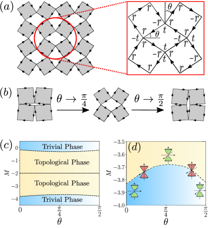
Figure 1: Model and Phase Diagram: (a) Schematic of the Kirigami network made up of square blocks. Each block is a Chern insulator (see eqn. (1)) hosting edge states. The zoomed region shows the effective unit cell and the convention of scattering matrix elements $r$ and $t$. 2$\theta$ is the inter-block angle. (b) Schematic of the network as a function of $\theta$ for $\theta\sim 0,\frac{\pi}{4}$ and $\frac{\pi}{2}$. (c) Numerically obtained phase diagram of the system as a function of $\theta$ and $M$. (d) Zoomed region of (c) near $M\sim-3.8$. The critical dashed line corresponds to $r(\theta)=t(\theta)$. Here the effective dispersion of the network undergoes a Dirac cone closing such that the blue (yellow) corresponds to the trivial (topological) phase.

Model: We model the Kirigami with a periodic arrangement of blocks with associated nodes governed by scattering matrices. We consider the microscopic Hamiltonian governing each of the blocks to the paradigmatic Bernevig-Hughes-Zhang (BHZ) model Bernevig et al. (2006). The Hamiltonian in momentum space is given by

$$H_{k_{x},k_{y}}=\sin(k_{x})\sigma_{x}+\sin(k_{y})\sigma_{y}+(M+2-\cos k_{x}-\cos k_{y})\sigma_{z}$$ (1)

where $M$ is the parameter which tunes topological and trivial phases such that for $M>0$ and $M<-4$ we have a trivial phase, while for $0>M>-2$ and $-2>M>-4$ we have Chern insulating phases with Chern number 1 and -1 respectively. All parameters are measured in terms of the bare hopping scale which is set to unity. All through this work we will assume that the lattice constant $a$ is set to unity and is much smaller than the typical size of the block such that each block by itself can be considered a thermodynamically large system. When $M$ is such that any block is in a topological phase the bulk of the each block remains gapped while the low-energy excitations are chiral and are present only on the boundaries. In particular Chern number $C=-1$ ($C=1$) phase leads to clockwise (anticlockwise) edge states. Thus the junction between adjoining blocks are governed by a scattering matrix between the edge states, which we discuss next.

Any node in this network is composed of two incoming ($1,3$) and two outgoing channels ($2,4$) (see Fig. 2(a) inset). Thus the scattering matrix $S$ is defined by two parameters $r$ and $t$ which are in general $\theta$ dependent, such that

$$\begin{pmatrix}\Psi_{2}\\ \Psi_{4}\end{pmatrix}=S\begin{pmatrix}\Psi_{1}\\ \Psi_{3}\end{pmatrix}\textrm{where}\quad S=\begin{pmatrix}-r&t\\ t&r\end{pmatrix}$$ (2)

where $|r|^{2}+|t|^{2}=1$ Kramer et al. (2005). In general $r,t$ are complex amplitudes, which we will choose to be real numbers and discuss later on the effect of phases. To estimate the functional behavior of $r,t$ on $\theta$ we use multiple methods discussed next.

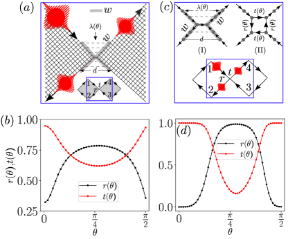
Figure 2: Junction physics: (a) Schematic showing that an incident electronic wave packet (from edge channel 1) on a node, gets reflected (on channel 2) and transmitted (on channel 3) by scattering matrix elements $r$ and $t$ respectively. $\lambda(\theta)$ is inter-edge hopping amplitude between sites separated by a distance $d(\theta)$ within a width $w$. (b) Behavior of $r(\theta),t(\theta)$ as a function of $\theta$ using wave-packet dynamics (see text) for $M=-3.6,\alpha=1,\beta=1,w=5,N=1250$. Here $N$ is the total number of sites in both the blocks forming the junction. (c) Schematics of a one-dimensional non-Hermitian system which also models the node and scattering physics. In (I) similar inter-edge coupling is introduced as in (a) to obtain $r(\theta),t(\theta)$ while in (II) the node itself is replaced by four sites with intersite non-Hermitian hoppings $r(\theta)$ and $t(\theta)$. (d) Behavior of $r(\theta)$ and $t(\theta)$ with $\theta$ using wave-packet dynamics on non-Hermitian system (I) ($\alpha=1.5,\beta=0.25,w=5$). Using these obtained $r,t$ in the model (II), reproduces the same curve (not shown).

Wave-packet dynamics: A state localized on a single site on the edge is initially projected in the low energy subspace $|E|<\Delta_{g}$ where $\Delta_{g}$ is the bulk gap in the topological regime. This leads to a finite projection into the chiral edge state which moves unidirectionally under time evolution (see schematic in Fig. 2(a), and Supplemental Material (SM) sup for details). After the packet leaves the junction the individual probability densities on the edges (2,4) given by $p_{2}$ and $p_{4}$ are evaluated numerically. This leads to $r\propto\sqrt{p_{2}}$ and $t\propto\sqrt{p_{4}}$ with a normalization constraint $r^{2}+t^{2}=1$. In the microscopic dynamics, in order to realistically model a smooth junction we introduce weak inter-block hoppings where fermions can hop from edges facing each other by an exponentially falling hopping amplitude $\lambda(\theta)=\alpha\exp(-\beta d(\theta))$ where $\alpha,\beta$ allows us to modulate the coupling between edges and $d(\theta)$ is the distance between two sites on the facing edges within a finite range $w$ of the Kirigami junction (see Fig. 2(a)). Here we fix $\alpha,\beta=1,w=5$ unless mentioned otherwise. Choosing $M=-3$ which is deep in the topological phase with Chern number $C=-1$ (clockwise edge states) we evaluate $r,t$ for all values of $\theta$. We find an intriguing dependence, where $t(\theta)\sim 1$ near both $\theta\sim 0$ and $\sim\frac{\pi}{2}$ while $r(\theta)>t(\theta)$ near $\theta\sim\frac{\pi}{4}$ (see Fig. 2(b)). We have checked that this behavior is independent of the system size (see SM sup ). We note that the exact values depend on the choice of $\lambda(\theta),w$, and $M$, however, the qualitative behavior of these coefficients do not sup . This motivates us to present an effective one-dimensional edge model to qualitatively capture the physics of this junction.

Effective non-Hermitian chain: In order to capture the effective scattering of the one-dimensional edge mode we model the chiral edge state with a one-dimensional Hatano-Nelson model Hatano and Nelson (1996, 1997) where the fermions are allowed to hop in just one direction. This uses the mapping of boundary theories of $d$ dimensional topological phases to $d-1$ dimensional non-Hermitian systems Lee et al. (2019); Lieu (2018); Shen et al. (2018); Schindler et al. (2023); more physically such a scattering mapping prevents any backscattering from the junction as is true for chiral systems. To make this connection more concrete, we consider the case where we wish to model the effective Hamiltonian of just a chiral edge state: $H_{\text{edge}}\sim v_{F}kc^{\dagger}_{k}c_{k}$ where $v_{F}$ is the edge state Fermi velocity. A non-Hermitian Hatano-Nelson (HN) Hamiltonian of the form

$$H_{\text{edge}}=\sum_{i}-c^{\dagger}_{i+1}c_{i}$$ (3)

where $i$ runs over the one-dimensional chain, stabilizes a unidirectional finite current at finite densities in a steady state mimicking a chiral edge state Hatano and Nelson (1997); Lee et al. (2019); Banerjee et al. (2022). We thus model the junction using an effective non-Hermitian system. We use four one-dimensional HN chains to form a junction with non-reciprocal hoppings in the direction of the edge currents as shown in Fig. 2(c, I). Similar to the BHZ system, interchain couplings are added in form of $\lambda(\theta)$. Again doing a wavepacket evolution we calculate $r(\theta),t(\theta)$ which is shown in Fig. 2(d). The qualitative similarity between (b) and (d) shows that the non-Hermtian scattering junction is indeed able to capture the scattering physics of the microscopic BHZ system. Interestingly, $r(\theta),t(\theta)$ can themselves be interpreted as a parameter to define another non-Hermitian junction as shown in Fig. 2(c, II) which subsumes the other particulars of the junction leading to identical reflection and transmission amplitudes. These results, taken together, illustrate that the scattering amplitudes are indeed dependent on the angle of the junction between each of the Kirigami blocks independent of microscopic parameters or modelling protocols.

Chalker Coddington networks: Having defined the property of every junction we discuss the phases realized due to the complete Kirigami network. The effective hopping problem due to the transfer matrix can be designed as a unitary evolution where an initial state evolves as Charles et al. (2020)

$$|\Psi_{f}\rangle=U_{\text{eff}}|\Psi_{i}\rangle$$ (4)

where the effective evolution operator, $U_{\text{eff}}$ is decided by the scattering matrix structure of the network (see SM sup ). The $U_{\text{eff}}$ is constructed using a median lattice where each edge of the Kirigami block is replaced by a site such that the system has a 16-site unit cell. The ‘hopping’ elements are represented by $r(\theta)$ and $t(\theta)$ with appropriate convention depending on the direction of the edge current. Given the network is translationally invariant, in order to see if it retains any edge states we set it up on a ribbon geometry which is finite in the $y$ direction and periodic in the $x$ direction. We find the eigenvalues of $U_{\text{eff}}$ which are of the form $e^{-i\epsilon}$ and plot $\epsilon$ as a function of $k_{x}$. Note that $r,t$ enter as parameters in the transfer matrix.

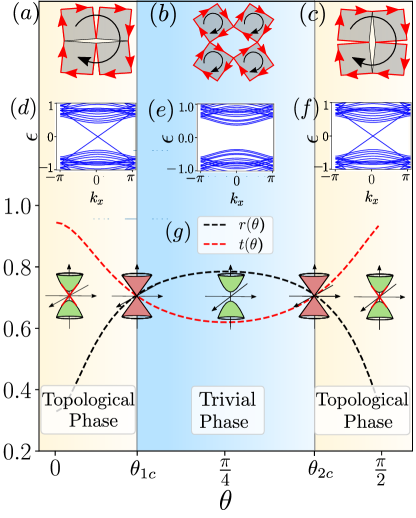
Figure 3: Network model: (a)-(c) Schematic of Kirigami network as function of angle for $\theta\sim 0,\frac{\pi}{4}$ and $\frac{\pi}{2}$. While each block contains edge states (red arrows), they hybridize to render the complete network topological in (a) and (c), and trivial in (b). (d)-(f) Behavior of eigenvalues $\epsilon$ of $i\ln(U_{\text{eff}})$ as a function of $k_{x}$ then the network is solved on a ribbon geometry where $y$ direction is kept open. Edge states are present when $0<\theta<\theta_{1c}$ (d) and $(\theta_{2c}<\theta<\frac{\pi}{2})$ (f) while the system is trivial between $(\theta_{1c}<\theta<\theta_{2c})$ (e). (g) The behavior of $r(\theta)$ (black dashed line) and $t(\theta)$ (red dashed line) as a function of $\theta$ for $N=1250,M=-3.6,\alpha=1,\beta=1,w=5$ along with schematic figures showing the bulk gap closings. Dirac cone closings happen at $\theta_{1c}$ and $\theta_{2c}$ when $r(\theta)=t(\theta)$.

When $r<t$ and $\theta<\theta_{1c}$, we find linearly dispersing edge states on the boundary (see Fig. 3(d)) reflecting that the topological character of the individual Kirigami block also leads to an overall chiral edge in the system (Fig. 3(a)). The edge state profile is shown in SM sup . However now as $\theta$ is increased, or the structure opens up, the individual scattering elements ($r(\theta),t(\theta)$) modulate approaching a critical point $\theta_{1c}$ where $r=t$. At this point, the system undergoes a phase transition where the $\epsilon$ shows a Dirac-like gap closing. After $\theta>\theta_{1c}$ the gap opens up again (Fig. 3(e)) albeit with no chiral mode on the complete network. This reflects that the Kirigami network has become a “trivial” insulator (see Fig. 3(b)). This is an example of a mechanical deformation-induced topological phase transition. With further increase in $\theta$ another critical point $\theta_{2c}$ is approached where the system transits back from the trivial to topological phase (see Fig. 3(c) and (f)). The specific values of $\theta_{1c}$ and $\theta_{2c}$ are dependent on both the microscopic parameters of the Hamiltonian governing each block, as well as the nature of the network. For instance in the case of the square network shown in Fig. 1(a), $\theta_{1c}$ and $\theta_{2c}$ are symmetric about $\pi/4$. For every value of $M$ numerically evaluated $r=t$ points leads to the phase diagram as shown in Fig. 1(c),(d). While we have chosen $r,t$ to be real, a uniform phase does not change $\theta_{1c},\theta_{2c}$. However relative scattering phase either uniform, or randomly varying from block to block can lead to both changes in critical angles and new phases Charles et al. (2020) which we do not explore here but is an interesting future direction.

We note that this analysis and formalism is only applicable when each of the Kirigami blocks resides in the topological regime i.e. $-4<M<0$. For other values of $M$ when each of the blocks is itself an insulator - mechanical deformation doesn’t render it topological. Within $-4<M<0$ each block has a topological phase transition at $M=0,-2$, and $-4$ where the system contains Dirac cones. Here again, the blocks are themselves metallic and this analysis breaks down. Given the $M=-2$ point sits between the two topological Chern insulator phases of Chern number $\pm 1$, $r=t$ by symmetry reasons. Overall the phase diagram is further symmetric about $M=-2$ since apart from the direction of the chiral edge states the physics remains the same.

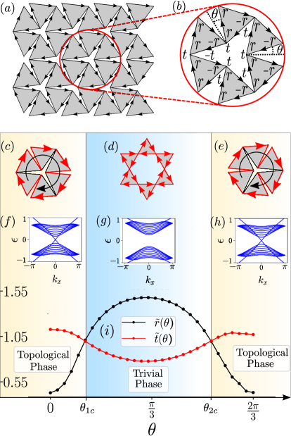
Figure 4: Triangular network Kirigami:  (a) Schematic of the Kirigami network made up of triangular blocks and the corresponding convention of scattering matrix elements is shown in (b). (c)-(e) Schematic of the network at $\theta\sim 0,\frac{\pi}{3}$ and $\frac{2\pi}{3}$. Each triangular block containing the edge states (red arrows) corresponds to the topological phase of the network as shown in (c) and (e), and the trivial phase in (d). The ribbon geometric calculation of the network with periodic in $x$ and open in $y$ direction shows the energy eigenvalues as a function of $k_{x}$ in (f)-(h). The edge states are present when $0<\theta<\theta_{1c}$ (f) and $(\theta_{2c}<\theta<\frac{2\pi}{3})$ (h) while the system is trivial between $(\theta_{1c}<\theta<\theta_{2c})$ (g). (i) The behavior of $\tilde{r}(\theta)$ (black line) and $\tilde{t}(\theta)$ (red line) as function of $\theta$ for $N=256,M=-3.5,\alpha=2,\beta=1,w=3$.

It is interesting to point out the physics of the $r=t$ line in this system, particularly near $\theta\sim 0$. Given when each Kirigami block is in the topological regime - there exists an edge state with an edge localization length $\xi$, which is dependent on the bulk gap which in turn depends on $M$. Thus whether an edge wavepacket can transmit or reflect from the junction depends on whether $\xi\ll w$ or $\xi\gg w$ respectively. Therefore given a choice of $w$, there exists a critical value of $M$ even within the topological phase, defined as $M^{*}$ at which $\xi(M)\sim w$, therefore leading to a point where $r=t$. This value of $M^{*}$ is thus independent of the system size of the Kirigami block but only dependent on the value of $\theta$ and the parameters defining the junction. We further note tuning $\alpha,\beta$ which defines the strength of the junction can further tune the values of $r,t$ (see SM sup ).

In order to test this physics in another network, we set up the same problem however now on a Kirigami network where the network deforms between the triangular lattice to a Kagome-like network as a function of deformation angle $\theta$ (see Fig. 4(a),(b)). The microscopic Kirigami block is still assumed to be governed by a square lattice BHZ model. Given a different network structure the $U_{\text{eff}}$ changes. However again as a function of $\theta$ the system undergoes topological to trivial to topological phase transitions as shown in (see Fig. 4(c)-(e). What is interesting however is that the critical points $\theta_{1c}$ and $\theta_{2c}$ are now symmetric about $\theta=\frac{\pi}{3}$. Moreover the topological transition occurs at $r(\theta)=\frac{1}{2},t(\theta)=\frac{\sqrt{3}}{2}$. Thus the transitions can be found when $\tilde{r}(\theta)=\tilde{t}(\theta)$ where $\tilde{r}(\theta)\equiv 2r(\theta)$ and $\tilde{t}(\theta)\equiv\frac{2}{\sqrt{3}}t(\theta)$. The behavior of $\tilde{r}(\theta)$ and $\tilde{t}(\theta)$ for $M=-3.5$ is shown in Fig. 4(i). The spectrum when evaluated on a ribbon geometry clearly shows the edge states in the topological regimes (see Fig. 4(f-h)). This reflects the generality of this physics to various Kirigami systems and that critical angles for transitions can themselves be tuned by nature of the Kirigami structure.

Outlook: Metamaterials and mechanically engineered systems herald the new era of technological devices. A host of electronic systems based on such structures have been realized. However, the interplay of quantum phases and their transitions vis-a-vis their mechanical tunability has been little explored. In this work, we show that topological phases, in particular a Chern insulator which contains chiral edge channels can be tuned to a trivial phase by such mechanical tuning. Recent experimental progress, in particular, such Kirigami-based systems Jin and Yang have significantly expanded the capabilities to realise this physics. Our study places this idea on a concrete footing in the context of topological phases uncovering their mechanism in a simple setting. The effect of realistic strains, gradients in deformations, strong correlations, and interactions are some of the many future directions this work opens up. Equivalent physics in alternate platforms such as photonics and phononic systems may be another interesting direction to pursue.

Acknowledgement: We acknowledge fruitful discussions with G. Murthy, G. Sreejith, Diptarka Das, Arijit Kundu, Subrata Pachhal, Sudipta Dubey, Ritajit Kundu, Saikat Mondal and Soumya Sur. RS acknowledges funding from IIT Kanpur Institute Fellowship. AA acknowledges support from IITK Initiation Grant (IITK/PHY/2022010).

Supplemental Material for “Tunable Topological Phases in Quantum Kirigamis”

In this SM we discuss the numerical procedure to estimate $r(\theta),t(\theta)$ and present additional results on their dependence on various model parameters.

I Wave packet evolution and estimation of $r(\theta),t(\theta)$

We study the junction by first choosing two finite sized square lattices (describing two Kirigami blocks) each of size $L\times L$ such that the total number of sites are $N=2L^{2}$. Every site has two orbitals $A,B$ such that the total number of fermionic orbitals is $2N$. The Hamiltonian describing these two blocks separately is $H_{\text{BHZ}}$ and that describing the couplings between these two blocks is $\equiv H_{\text{coupling}}$. Thus the total Hamiltonian of the system is given by,

$$H=H_{\rm{BHZ}}+H_{\rm{coupling}}$$ (S1)

$H_{\text{BHZ}}$: Within every Kirigami block the hopping Hamiltonian is given by

$$H_{\text{BHZ}}=\sum_{i,\delta}\Psi^{\dagger}_{i}T_{\delta}\Psi_{i+\delta}+\text{h.c.}+\sum_{i}\Psi^{\dagger}_{i}\Gamma\Psi_{i}$$ (S2)

where $\delta=\hat{x},\hat{y}$, the unit vectors in the $x$ and $y$ directions defined with respect to a local axis defined for every Kirigami block. $\Psi_{i}\equiv\Big{(}c_{iA},c_{iB}\Big{)}^{T}$ where $c_{iA},c_{iB}$ are the fermionic annihilation operators corresponding to the two orbitals $A,B$ at site $i$. $\Gamma$ describes the onsite energies and $T_{\hat{x}}$ and $T_{\hat{y}}$ are the hopping matrices given by:

$$T_{\hat{x}}=-\frac{1}{2}(\sigma_{z}+i\sigma_{x}),T_{\hat{y}}=-\frac{1}{2}(\sigma_{z}+i\sigma_{y}),\Gamma=(M+2)\sigma_{z}$$ (S3)

In a translationally invariant system, this Hamiltonian in the momentum space gives rise to eqn. (1) in the main text. Note that as the angle $\theta$ is changed, such that the local coordinate system of every Kirigami block obtains a relative angle with respect to another Kirigami block, the hopping amplitudes within any Kirigami block does not change. For instance as shown in Fig. S1 the relative angle between the two Kirigami blocks with local coordinates $(x,y)$ and $(x^{\prime},y^{\prime})$ respectively has a mutual angle of $2\theta$.

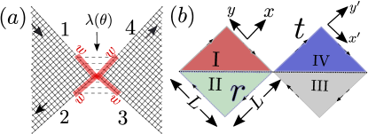
Figure S1: Model: (a) A junction is modelled with two square Kirigami blocks meeting at a node. The interblock couplings are limited to a width $w$ and has a angle dependent hopping of strength $\lambda(\theta)$. (b) While each block has a size $L\times L$, it has a local coordinate axis which rotates as a function of deformation angle. The Kirigami blocks can be divided into four regions I-IV to estimate the scattering matrix coefficients (see text).

$H_{\text{coupling}}$: Next we couple the two Kirigami blocks with interblock hoppings as follows. Labelling the sides (edges) forming the junction ($s_{e}$=1-4) as shown in Fig. S1(a), we identify the sites along the edges $n=1,2,\ldots w$. Thus $w$ number of sites, denoting the width of the edge, couple between the sides facing each other. For instance in Fig. S1(a), $s_{e}=1$ and $s_{e}=4$, and similarly $s_{e}=2$ and $s_{e}=3$. Labeling the fermionic creation operators on the edge $s_{e}$ at site $n$ as $\Psi^{\dagger}_{n,s_{e}}$, the $H_{\rm{coupling}}$ is therefore given by

$$\hat{H}_{\rm{coupling}}=\sum_{n=1}^{w}\lambda(n,\theta)\Big{(}\Psi^{\dagger}_{n,1}T_{\hat{x}}\Psi_{n,4}+\Psi^{\dagger}_{n,2}T_{\hat{x}}\Psi_{n,3}\Big{)}+\text{h.c.}$$ (S4)

The functional form of $\lambda(n,\theta)$ implements the interblock hopping amplitudes which we describe next. Given the two sites $n$ on $s_{e}=1$ and $s_{e}=4$ the distance between them is $d=2n\sin(\theta)$, and similarly for those between $s_{e}=2$ and $s_{e}=3$ is $d=2n\sin(\frac{\pi}{2}-\theta)$. Given a distance $d$ between the two facing sites, the hopping amplitude is given by

$$\lambda(\theta)=\alpha\exp(-\beta d(\theta))$$ (S5)

where $\alpha$ and $\beta$ are tuning parameters. We set $\alpha=1,\beta=1$ unless otherwise stated. The choice of parameters and the coupling Hamiltonian have been kept such that at $\theta=0$, $\lambda(\theta)=1$ thus the coupling reduces to the bare hopping scale of the rest of the BHZ system.

Having described the Hamiltonian of the system, we next discuss the wavepacket evolution and estimation of $r(\theta)$ and $t(\theta)$. Given a choice of $M$ and $\theta$, we first diagonalize $H$ (see eqn. (S1)) to obtain the complete eigenspectrum. In the gapped topological regime of the system, the bulk gap is given $\Delta_{g}(M)$. We form a projector out of the single particle wavefunctions $|m\rangle$ such that their eigen energies $\epsilon_{m}$ are $|\epsilon_{m}|<\Delta_{g}(M)$. The projector is thus given by

$$\hat{P}=\sum_{m,|\epsilon_{m}|<\Delta_{g}(M)}|m\rangle\langle m|$$ (S6)

This projects any wavefunction to the edge state manifold of the complete system.

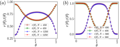
Figure S2: System size ($N$) dependence: (a) $r(\theta)$ and $t(\theta)$ in BHZ junction modelling (see Fig.2(a) of main text) when $N=450$ and $N=1250$ with $\alpha=1,\beta=1,w=5$ and $M=-3.6$. (b) $r(\theta)$ and $t(\theta)$ in Non-Hermitian junction modelling (see Fig.2(c) of main text) when $N=400$ and $N=560$ with $\alpha=1.5,\beta=0.25$ and $w=5$.

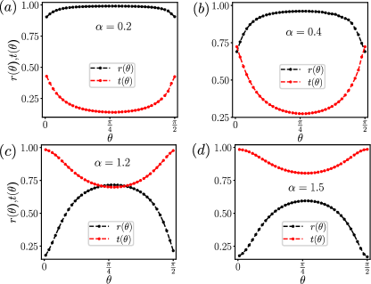
Figure S3: Coupling dependence:  $r(\theta)$ and $t(\theta)$ in BHZ junction modelling (see Fig.2(a) of main text) with ($N=1250$, $M=-3.6,\beta=1$ and $w=5$). (a) $\alpha=0.2$ corresponds to the $r\approx 1$ and $t\approx 0$. (b) For $\alpha=0.4$, $r=t$ when $\theta\approx 0$ or $\frac{\pi}{2}$. (c) For $\alpha=1.2$, $r=t$ when $\theta\approx\frac{\pi}{4}$. (d) For $\alpha=1.5$ $t(\theta)>r(\theta)$.

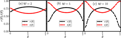
Figure S4: $w$ dependence: The junction width $(w)$ dependence of $r(\theta)$ and $t(\theta)$ in BHZ junction modelling (see Fig.2(a) of main text) with ($N=1250$, $\alpha=1,\beta=1$ and $M=-3.6$)

To start the wavepacket evolution we initialize a unit state on the top corner of the side 1 on the A orbital. We project this state using the projector above (see eqn. (S6)) and renormalize it to obtain the initial state $|\psi_{\text{in}}\rangle$. This state is further evolved using the Hamiltonian (see eqn. (S1)) to a later time such that final state $|\psi_{\text{fi}}\rangle$ at time $t$ is given by

$$|\psi_{\text{fi}}\rangle=\exp(-iHt)|\psi_{\text{in}}\rangle$$ (S7)

The initial packet moves towards the junction and scatters into edges 2 and 4. Given the unidirectional chiral edge states, there is neither any backscattering nor any amplitude on edge 3. After a time when the packet has scattered from the junction, we calculate the total probability density on the sides 2 and 4. To estimate the reflected probability density we evaluate

$$p_{2}=\sum_{i\in\rm{region~{}II},\gamma={A,B}}|\langle i\gamma|\psi_{\text{fi}}\rangle|^{2}$$ (S8)

and similarly the transmitted probability density is given by

$$p_{4}=\sum_{i\in\rm{region~{}IV},\gamma={A,B}}|\langle i\gamma|\psi_{\text{fi}}\rangle|^{2}$$ (S9)

The various regions (I-IV) are shown in Fig. S1. Consistent with the expectations we find that the corresponding quantities in regions III and I $p_{3}=p_{1}=0$ after the scattering event. Having estimate $p_{2}$ and $p_{4}$, we calculate $r(\theta)=\sqrt{p_{2}}$ and $t(\theta)=\sqrt{p_{4}}$. This procedure is repeated for various values of $M$ and $\theta$ to obtain the variations of $r(\theta),t(\theta)$ and the numerically obtain the phase diagrams as reported in the main text. The procedure remains the same for the triangular motif as well, where the Kirigami block is still a square lattice BHZ but the boundaries are formed into a triangular motif. Other parameters and the coupling Hamiltonian are kept the same.

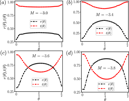
Figure S5: $M$ dependence: $M$ dependence of $r(\theta)$ and $t(\theta)$ in BHZ junction modelling (see Fig.2(a) of main text) with ($N=1250$, $\alpha=1,\beta=1$ and $w=5$).

II Parameter dependence of $r(\theta)$ and $t(\theta)$

In this section, we investigate and present additional results on the functional dependence of $r(\theta)$ and $t(\theta)$ on various parameters such as its system size ($N$), BHZ mass parameter $M$, width $w$ and coupling parameter $\alpha$.

System size ($N$) dependence: With the fixed set of parameters $(\alpha,\beta,w$ and $M$), we model the junction using both the microscopic BHZ junction and the effective $1d$ non-hermitian system. We find that the functional forms of $r(\theta)$ and $t(\theta)$ are independent of the system size ($N$) as shown in Fig. S2.

Coupling dependence $(\alpha,w)$: Given a set of parameters ($N,M,w$, and $\beta$) we find that tuning the coupling strength ($\alpha$) can lead a quantitative change of $r(\theta)$ and $t(\theta)$, as illustrated in Fig. S3. The smaller value of $\alpha$ reduces the junction strength impeding transmission thus resulting in $r(\theta)>t(\theta)$. Interestingly, we note that for $\alpha=0.4$, the junction shows $r=t$ when $\theta\approx 0$ and $\frac{\pi}{2}$. This corresponds to the critical angles $(\theta_{1c}$ and $\theta_{2c})$ (as mentioned in main text). By tuning $\alpha$ to $1.2$ one can tune these critical angles up to $\theta\approx\frac{\pi}{4}$ (Fig. S3(c)) Further, increase in $\alpha$ makes $t(\theta)>r(\theta)$ as shown in Fig. S3(d). Similarly tuning $w$ can allow further modulation of $r(\theta)$ and $t(\theta)$ as shown in Fig. S4. Thus $\alpha,w$ serve as important tuning parameters in the system.

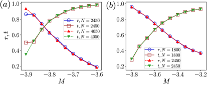
Figure S6: $M^{*}$ physics: (a) $r$ and $t$ as function of $M$ when $\theta=0$ with $N=2450$ and $N=4050$ with ($\alpha=1,\beta=1,w=5$). (b) $r$ and $t$ as function of $M$ when $\theta=\frac{\pi}{6}$ with $N=1800$ and $N=2450$ with ($\alpha=1,\beta=1,w=5$)

$M$ dependence: The localization length $\xi$ of the edge states is related to $M$. Deep in a topological phase when $M=-3$ and a given $w=5$ the system has $\xi\ll w$ thus it allows easy transmission with $(t>r)$ as shown in Fig. S5(a) for all values of $\theta$. Note as $M$ is decreased further to $M=-3.6$ and $-3.8$, $\xi(M)$ increases since the bulk gap closing happens at $M=-4$. Given $t\sim 1$ near $\theta\sim 0$ implies that $\xi(M)<w$. However now in an intermediate range of $\theta$ near $\frac{\pi}{4}$ we find $r>t$. This increase in $r$ can be attributed to an effective reduction of junction coupling due to a coupling strength ($\lambda(\theta)$).

System size dependence of $M^{*}$: In Fig. S6 we show the system size dependence of $r,t$ as a function of $M$ for a fixed $\theta=0,\frac{\pi}{6}$. We find that the critical point $M^{*}$ (where $r=t$) is independent of the system size. We further note that near $M\sim-4$, where the bulk gap closes, system size needs to be significantly large to reduce finite size effects.

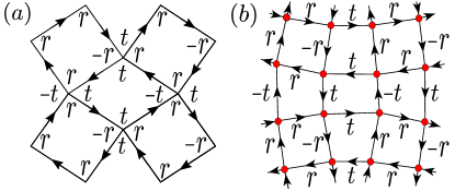
Figure S7: Median lattice: (a) Unit cell of Kirigami structure. (b) Median lattice of a unit cell of Kirigami structure.

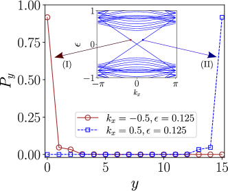
Figure S8: Edge state profile:  $P_{y}$ as function of $y$ when $L_{y}=16,r=0.4,t=0.916$. For (I) $k_{x}=-0.5,\epsilon=0.125$ and for (II) $k_{x}=0.5,\epsilon=0.125$

III $U_{\text{eff}}$ and edge states

In order to calculate the effective time evolution operator $U_{\text{eff}}$ of the complete network (see eqn. (4) of main text) one needs to form a median lattice of the Kirigami network. Such a lattice is constructed by replacing every side of the Kirigami block with a site placed in the middle and with hopping amplitudes that are unidirectional and follow the same convention of $r(\theta)$ and $t(\theta)$ as in the scattering junctions. The unit cell of the original Kirigami network and the corresponding median lattice is shown in Fig. S7. Fourier transforming this non-Hermitian Hamiltonian leads to the eigenvalues $e^{-i\epsilon}$, from which $\epsilon$ can be obtained. A similar calculation for the triangular motif leads to a six-site unit cell. The same problems are solved on a ribbon geometry, with periodic boundary conditions in the $x$ direction to give us the band dispersions as reported in the main text. Our treatment closely follows Charles et al. (2020).

Now we investigate the edge state profile of diagonalizing $U_{\text{eff}}$ on a ribbon geometry which has translational symmetry in the $x$ direction and is finite in the $y$ direction. The spectrum is shown in Fig. 3(d) and (f) in the main text. The electronic probability density $P_{y}$ (as a function of $y$) for given values of $k_{x}$ and $\epsilon$ is shown in Fig. S8. As can be seen, the right (left) moving edge state resides on the bottom (top) of the ribbon. These states are absent when periodic boundary conditions are used in the $y$ direction.

References

- Rogers et al. (2010) John A Rogers, Takao Someya, and Yonggang Huang, “Materials and mechanics for stretchable electronics,” science 327, 1603–1607 (2010).
- Blees et al. (2015) Melina K Blees, Arthur W Barnard, Peter A Rose, Samantha P Roberts, Kathryn L McGill, Pinshane Y Huang, Alexander R Ruyack, Joshua W Kevek, Bryce Kobrin, David A Muller, et al., “Graphene kirigami,” Nature 524, 204–207 (2015).
- Ouyang et al. (2023) Hongyi Ouyang, Yuanqing Gu, Zhibin Gao, Lei Hu, Zhen Zhang, Jie Ren, Baowen Li, Jun Sun, Yan Chen, and Xiangdong Ding, “Kirigami-inspired thermal regulator,” Phys. Rev. Appl. 19, L011001 (2023).
- Liu et al. (2018) Zhiguang Liu, Huifeng Du, Jiafang Li, Ling Lu, Zhi-Yuan Li, and Nicholas X Fang, “Nano-kirigami with giant optical chirality,” Science advances 4, eaat4436 (2018).
- (5) Lishuai Jin and Shu Yang, “Engineering kirigami frameworks toward real-world applications,” Advanced Materials n/a, 2308560.
- Castro et al. (2018) Eduardo V. Castro, Antonino Flachi, Pedro Ribeiro, and Vincenzo Vitagliano, “Symmetry breaking and lattice kirigami,” Phys. Rev. Lett. 121, 221601 (2018).
- Flachi and Vitagliano (2019) Antonino Flachi and Vincenzo Vitagliano, “Symmetry breaking and lattice kirigami: Finite temperature effects,” Phys. Rev. D 99, 125010 (2019).
- Imaki and Yamamoto (2019) Shota Imaki and Arata Yamamoto, “Lattice field theory with torsion,” Phys. Rev. D 100, 054509 (2019).
- Grosso and Mele (2015) Bastien F. Grosso and E. J. Mele, “Bending rules in graphene kirigami,” Phys. Rev. Lett. 115, 195501 (2015).
- Hanakata et al. (2018) Paul Z. Hanakata, Ekin D. Cubuk, David K. Campbell, and Harold S. Park, “Accelerated search and design of stretchable graphene kirigami using machine learning,” Phys. Rev. Lett. 121, 255304 (2018).
- Liu et al. (2022) Lucy Liu, Gary P. T. Choi, and L. Mahadevan, “Quasicrystal kirigami,” Phys. Rev. Res. 4, 033114 (2022).
- Bahamon et al. (2016) D. A. Bahamon, Zenan Qi, Harold S. Park, Vitor M. Pereira, and David K. Campbell, “Graphene kirigami as a platform for stretchable and tunable quantum dot arrays,” Phys. Rev. B 93, 235408 (2016).
- Mortazavi et al. (2017) Bohayra Mortazavi, Aurélien Lherbier, Zheyong Fan, Ari Harju, Timon Rabczuk, and Jean-Christophe Charlier, “Thermal and electronic transport characteristics of highly stretchable graphene kirigami,” Nanoscale 9, 16329–16341 (2017).
- Ludwig (2016) Andreas W W Ludwig, “Topological phases: classification of topological insulators and superconductors of non-interacting fermions, and beyond,” Physica Scripta 2016, 014001 (2016).
- Chiu et al. (2016) Ching-Kai Chiu, Jeffrey C. Y. Teo, Andreas P. Schnyder, and Shinsei Ryu, “Classification of topological quantum matter with symmetries,” Rev. Mod. Phys. 88, 035005 (2016).
- Hasan and Kane (2010) M. Z. Hasan and C. L. Kane, “Colloquium : Topological insulators,” Rev. Mod. Phys. 82, 3045–3067 (2010).
- Qi and Zhang (2011) Xiao-Liang Qi and Shou-Cheng Zhang, “Topological insulators and superconductors,” Rev. Mod. Phys. 83, 1057–1110 (2011).
- Asbóth et al. (2016) János K Asbóth, László Oroszlány, and András Pályi, “A short course on topological insulators,” Lecture notes in physics 919, 166 (2016).
- Chalker and Coddington (1988) JT Chalker and PD Coddington, “Percolation, quantum tunnelling and the integer hall effect,” Journal of Physics C: Solid State Physics 21, 2665 (1988).
- Ho and Chalker (1996) C.-M. Ho and J. T. Chalker, “Models for the integer quantum hall effect: The network model, the dirac equation, and a tight-binding hamiltonian,” Phys. Rev. B 54, 8708–8713 (1996).
- Kramer et al. (2005) Bernhard Kramer, Tomotada Ohtsuki, and Stefan Kettemann, “Random network models and quantum phase transitions in two dimensions,” Physics reports 417, 211–342 (2005).
- Lee et al. (1993) Dung-Hai Lee, Ziqiang Wang, and Steven Kivelson, “Quantum percolation and plateau transitions in the quantum hall effect,” Phys. Rev. Lett. 70, 4130–4133 (1993).
- Snyman et al. (2008) I. Snyman, J. Tworzydło, and C. W. J. Beenakker, “Calculation of the conductance of a graphene sheet using the chalker-coddington network model,” Phys. Rev. B 78, 045118 (2008).
- Cho and Fisher (1997) Sora Cho and Matthew P. A. Fisher, “Criticality in the two-dimensional random-bond ising model,” Phys. Rev. B 55, 1025–1031 (1997).
- Charles et al. (2020) N. Charles, I. A. Gruzberg, A. Klümper, W. Nuding, and A. Sedrakyan, “Critical behavior at the integer quantum hall transition in a network model on the kagome lattice,” Phys. Rev. B 102, 121304 (2020).
- Potter et al. (2020) Andrew C. Potter, J. T. Chalker, and Victor Gurarie, “Quantum hall network models as floquet topological insulators,” Phys. Rev. Lett. 125, 086601 (2020).
- Obuse et al. (2012) Hideaki Obuse, Ilya A. Gruzberg, and Ferdinand Evers, “Finite-size effects and irrelevant corrections to scaling near the integer quantum hall transition,” Phys. Rev. Lett. 109, 206804 (2012).
- Hu et al. (2015) Wenchao Hu, Jason C. Pillay, Kan Wu, Michael Pasek, Perry Ping Shum, and Y. D. Chong, “Measurement of a topological edge invariant in a microwave network,” Phys. Rev. X 5, 011012 (2015).
- Chalker et al. (2001) J. T. Chalker, N. Read, V. Kagalovsky, B. Horovitz, Y. Avishai, and A. W. W. Ludwig, “Thermal metal in network models of a disordered two-dimensional superconductor,” Phys. Rev. B 65, 012506 (2001).
- De Beule et al. (2021) Christophe De Beule, Fernando Dominguez, and Patrik Recher, “Network model and four-terminal transport in minimally twisted bilayer graphene,” Phys. Rev. B 104, 195410 (2021).
- Bernevig et al. (2006) B Andrei Bernevig, Taylor L Hughes, and Shou-Cheng Zhang, “Quantum spin hall effect and topological phase transition in hgte quantum wells,” science 314, 1757–1761 (2006).
- (32) See supplemental material for additional details.
- Hatano and Nelson (1996) Naomichi Hatano and David R. Nelson, “Localization transitions in non-hermitian quantum mechanics,” Phys. Rev. Lett. 77, 570–573 (1996).
- Hatano and Nelson (1997) Naomichi Hatano and David R. Nelson, “Vortex pinning and non-hermitian quantum mechanics,” Phys. Rev. B 56, 8651–8673 (1997).
- Lee et al. (2019) Jong Yeon Lee, Junyeong Ahn, Hengyun Zhou, and Ashvin Vishwanath, “Topological correspondence between hermitian and non-hermitian systems: Anomalous dynamics,” Phys. Rev. Lett. 123, 206404 (2019).
- Lieu (2018) Simon Lieu, “Topological phases in the non-hermitian su-schrieffer-heeger model,” Phys. Rev. B 97, 045106 (2018).
- Shen et al. (2018) Huitao Shen, Bo Zhen, and Liang Fu, “Topological band theory for non-hermitian hamiltonians,” Phys. Rev. Lett. 120, 146402 (2018).
- Schindler et al. (2023) Frank Schindler, Kaiyuan Gu, Biao Lian, and Kohei Kawabata, “Hermitian bulk – non-hermitian boundary correspondence,” PRX Quantum 4, 030315 (2023).
- Banerjee et al. (2022) Ayan Banerjee, Suraj S. Hegde, Adhip Agarwala, and Awadhesh Narayan, “Chiral metals and entrapped insulators in a one-dimensional topological non-hermitian system,” Phys. Rev. B 105, 205403 (2022).