[a]V. Martínez-Fernández
Double DVCS amplitudes including kinematic twist-3 and 4 corrections
Abstract
Generalized parton distributions (GPDs) are off-forward matrix elements of quark and gluon operators that work as a window to the total angular momentum of partons and their transverse imaging (nucleon tomography). To access GPDs one needs to look into exclusive processes which are usually studied in a kinematic regime known as the Björken limit. In this limit, the photon virtualities are much larger than the hadron mass , and the kick to the hadron measured by the Mandelstam’s variable . It turns out that this is not enough for the purposes of a precise GPD extraction and, in particular, of nucleon tomography for which measurements in a sizable range of are required. Deviation with respect to the Björken limit induces kinematic higher-twist corrections which enter the amplitudes with powers of and , where denotes the scale of the process (basically, the sum of photon virtualities in the case of DDVCS). There are also corrections by the name of “genuine” higher twists which are a separate topic and are not the subject of this research study.
In this manuscript, we present novel calculations of DDVCS amplitudes off a (pseudo-)scalar target including up to kinematic twist-4 corrections. These results are important for measuring DDVCS, DVCS and TCS through the Sullivan process and off helium-4 target at the future Electron-Ion Collider (EIC) and JLab experiments. Preliminary numerical estimates for the pion target are provided.
1 Introduction
Generalized parton distributions (GPDs) are off-forward matrix elements of quark and gluon operators that appear in the scattering amplitudes for deep exclusive processes. They constitute a 3D version of the usual one-dimensional parton distribution function (PDF). For a quark of flavor in a spin-0 hadron, there is only one chiral-even leading-twist GPD that is defined as:
| (1) |
where represents a Wilson line, is the so-called skewness and the vector is the usual lightlike vector projecting the positive-longitudinal component in light-cone coordinates. Also, .
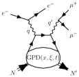
Double deeply virtual Compton scattering (DDVCS, illustrated in Fig. 1) [1, 2, 3, 4]:
| (2) |
contributes to the exclusive electroproduction of a lepton pair off a hadron , which in the muon channel is given by the reaction
| (3) |
This process also receives contributions from the purely QED Bethe-Heitler processes (BH), which do not provide access to GPDs. Hence, they are not affected by the twist expansion and will be ignored in what follows. See Refs. [2, 3, 4] for details on BH and its interplay with DDVCS regarding the cross-section and observables of the reaction (3) for a spin-1/2 target .
Other related processes are deeply virtual Compton scattering (DVCS) [5, 6, 7] and timelike Compton scattering (TCS) [8]. These two can be described under the formalism of DDVCS: taking the appropriate small virtuality limit, one recovers DVCS and TCS from DDVCS results [4].
DDVCS factorizes by means of GPDs and perturbatively calculable hard-coefficient functions when the scale of the process (basically, the sum of photon virtualities, with and ) is large enough: . This kinematic leading twist (LT) approximation is then applied to the Compton tensor
| (4) |
to get the LT DDVCS amplitude where GPDs enter by means of Compton form factors (CFFs) defined, at leading order (LO) in , as
| (5) |
where is the C-even part of the GPD weighted by the squared fractional quark electric charges:
| (6) |
Also, in Eq. (5), the generalized Björken variable has been introduced as .
Current and future experimental data cannot be considered as a trustworthy realization of the and limits. Therefore, corrections accounting for these effects need to be included and are referred to as kinematic higher-twist corrections, involving the leading-twist GPDs. There are also “genuine” higher twist corrections involving new GPDs, which are a separate topic and are not considered here. One can relate the kinematic corrections to the deviations with respect to the light-cone dominance of the Compton tensor (4). With this idea in mind and taking into account that at LO QCD is a conformal field theory (CFT),111Beyond LO, QCD is a conformal field theory at the Fisher-Wilson fixed point of the function. Working at said point and using the renormalization group equations, one can obtain correct results for QCD at four dimensions beyond LO. For further details, cf. [9] for example. V. M. Braun et al. developed an all kinematic-twist expansion of said tensor in Refs. [10, 11]. This methodology is briefly described in the next section.
2 Conformal operator-product expansion and the scale of DDVCS
Making use of the shadow-operator formalism of CFTs, cf. [12], one can obtain a close expression for the LO Compton tensor valid to all kinematic twists. For illustration purposes, some of the most light-cone divergent terms are given by
| (7) |
where symbols above are to be understood as matrix elements of the corresponding operators, i.e.
| (8) |
and
| (9) |
for the parameters of the usual double distributions (DDs) [7], which are related to the function as
| (10) |
By we refer to the geometric LT projection which reduces an operator to its symmetric and traceless component. Such a projector is described in Ref. [13].
After performing the Fourier transform of the different components of the geometric LT projection of the exponential in (8), one is left with integrals of the form
| (11) |
The structure of these integrals suggests the scale for any two-photon process to be , as and . The factor in could be dropped as it produces corrections of the next twist. Therefore, the twist expansion comes in powers of , whereas .
In the next section, we apply these techniques to DDVCS off a spin-0 target.
3 Scalar and pseudo-scalar target
The calculation of twist corrections can be organized by means of the so-called helicity-dependent amplitudes which are the amplitudes for transition between an incoming photon with helicity to an outgoing photon with helicity , where . The (helicity-dependent) CFFs of the hadron are related to them by . Therefore, the Compton tensor can be parameterized in terms of these amplitudes through:
| (12) |
where , and due to parity conservation. From this expression, a set of projectors onto the different can be read out and applied to Eq. (2). Let us now present as an example, together with preliminary results on its magnitude.
3.1 Example: transverse-helicity flip amplitude,
The transverse-helicity flip amplitude () is of a special interest as it may contribute to the cross-section in two ways: i) at LO as a higher-twist contribution, and ii) at NLO via gluon transversity GPDs [14]. We stay at LO, therefore starts at kinematic twist-4 and we obtain
| (13) |
where , and
| (14) |
for which the DVCS and TCS limits take the form:
| (15) |
Our calculation agrees in the DVCS limit with previous works [11] and with the DVCS-TCS connection discussed in [15].
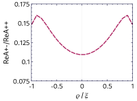
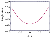
3.2 Numerical estimates of
We compare in Fig. 2 the numerical estimate of the real and imaginary parts of the amplitude with the leading-twist contribution to the Compton tensor, which comes solely from the transverse-helicity conserving amplitude . We use the phenomenological pion-GPD model described in Ref. [16]. The extreme left ( and right () values of the horizontal axes represent the TCS and DVCS limits, respectively. We observe that is of the order of with respect to for , which should be a measurable effect in DVCS as well as future TCS experiments.
Acknowledgements. The works of V.M.F. are supported by PRELUDIUM grant 2021/41/N/ST2/00310 of the Polish National Science Centre (NCN).
References
- [1] A. V. Belitsky and D. Müller, Exclusive electroproduction of lepton pairs as a probe of nucleon structure, Phys. Rev. Lett. 90 (2003) 022001.
- [2] A. V. Belitsky and D. Müller, Probing generalized parton distributions with electroproduction of lepton pairs off the nucleon, Phys. Rev. D 68 (2003) 116005 [hep-ph/0307369].
- [3] M. Guidal and M. Vanderhaeghen, Double deeply virtual compton scattering off the nucleon, Phys. Rev. Lett. 90 (2003) 012001 [hep-ph/0208275].
- [4] K. Deja, V. Martinez-Fernandez, B. Pire, P. Sznajder and J. Wagner, Phenomenology of double deeply virtual Compton scattering in the era of new experiments, Phys. Rev. D 107 (2023) 094035 [2303.13668].
- [5] D. Müller, D. Robaschik, B. Geyer, F. M. Dittes and J. Hořejši, Wave functions, evolution equations and evolution kernels from light ray operators of QCD, Fortsch. Phys. 42 (1994) 101 [hep-ph/9812448].
- [6] X.-D. Ji, Deeply virtual Compton scattering, Phys. Rev. D 55 (1997) 7114 [9609381].
- [7] A. V. Radyushkin, Symmetries and structure of skewed and double distributions, Phys. Lett. B 449 (1999) 81 [hep-ph/9810466].
- [8] E. R. Berger, M. Diehl and B. Pire, Time - like Compton scattering: Exclusive photoproduction of lepton pairs, Eur. Phys. J. C23 (2002) 675 [hep-ph/0110062].
- [9] V. M. Braun, A. N. Manashov, S. Moch and M. Strohmaier, Two-loop conformal generators for leading-twist operators in QCD, JHEP 03 (2016) 142 [1601.05937].
- [10] V. M. Braun, Y. Ji and A. N. Manashov, Two-photon processes in conformal QCD: resummation of the descendants of leading-twist operators, JHEP 03 (2021) 051 [2011.04533].
- [11] V. M. Braun, Y. Ji and A. N. Manashov, Next-to-leading-power kinematic corrections to DVCS: a scalar target, JHEP 01 (2023) 078 [2211.04902].
- [12] S. Ferrara, A. F. Grillo, G. Parisi and R. Gatto, The shadow operator formalism for conformal algebra. Vacuum expectation values and operator products, Lett. Nuovo Cim. 4S2 (1972) 115.
- [13] B. Geyer, M. Lazar and D. Robaschik, Decomposition of nonlocal light cone operators into harmonic operators of definite twist, Nucl. Phys. B 559 (1999) 339 [hep-th/9901090].
- [14] A. V. Belitsky and D. Mueller, Off forward gluonometry, Phys. Lett. B 486 (2000) 369 [hep-ph/0005028].
- [15] D. Mueller, B. Pire, L. Szymanowski and J. Wagner, On timelike and spacelike hard exclusive reactions, Phys. Rev. D 86 (2012) 031502 [1203.4392].
- [16] J. M. M. Chávez, V. Bertone, F. De Soto Borrero, M. Defurne, C. Mezrag, H. Moutarde et al., Pion generalized parton distributions: A path toward phenomenology, Phys. Rev. D 105 (2022) 094012.