MSmix: An R Package for clustering partial rankings via mixtures of Mallows Models with Spearman distance

Marta Crispino, Cristina Mollica, Lucia Modugno MSmix: An R Package for clustering partial rankings via mixtures of Mallows Model with Spearman distance MSmix: Mallows Model with Spearman distance MSmix is a recently developed R package implementing maximum likelihood estimation of finite mixtures of Mallows models with Spearman distance for full and partial rankings. The package is designed to implement computationally tractable estimation routines of the model parameters, with the ability to handle arbitrary forms of partial rankings and sequences of a large number of items. The frequentist estimation task is accomplished via EM algorithms, integrating data augmentation strategies to recover the unobserved heterogeneity and the missing ranks. The package also provides functionalities for uncertainty quantification of the estimated parameters, via diverse bootstrap methods and asymptotic confidence intervals. Generic methods for S3 class objects are constructed for more effectively managing the output of the main routines. The usefulness of the package and its computational performance compared with competing software is illustrated via applications to both simulated and original real ranking datasets. Mallows model, partial rankings, mixture models, EM algorithm, Monte Carlo, Bootstrap mallows model, partial rankings, mixture models, em algorithm, monte carlo, bootstrap Marta Crispino
Department of Economics Statistics and Research
Bank of Italy, Rome, Italy


Cristina Mollica
Department of Statistical Sciences
Sapienza University of Rome, Italy


Lucia Modugno
Department of Economics, Statistics and Research
Bank of Italy, Rome, Italy

1 Introduction

Ranking data play a pivotal role in numerous research and practical domains, serving as a means to compare and order a set of $n$ items according to personal preferences or other relevant criteria. From market analysis to sports competitions, from academic assessments to online recommendation systems, rankings are ubiquitous in modern society to capture human choice behaviors or, more generally, ordinal comparison processes in various contexts.

The Mallows model (MM) is a widely-used probabilistic framework for modeling and analyzing ranking data, and is also recognised as a useful parametric tool for rank aggregation tasks (Marden1995). It is grounded on the assumption that in the population there exists a modal consensus ranking of the $n$ items which best captures the collective preferences. The probability of observing any given ranking decreases as its distance from the consensus increases. Traditionally, the choice of the distance in defining the MM was driven by computational considerations, particularly the availability of the model normalizing constant (or partition function) in a closed form. This favored the use of Kendall, Cayley, and Hamming metrics while the Spearman distance has been poorly investigated due to its perceived intractability, despite representing a meaningful choice in preference domains and rank-based approaches (crispino23efficient). In fact, crispino23efficient recovered the effectiveness of the Spearman distance in the MM as an adequate metric joining both computational feasibility and interpretability. By leveraging the properties of the Spearman distance, and by means of a novel approximation of the model partition function, the authors addressed the critical inferential challenges that traditionally limited the use of the Spearman distance. This enabled them to propose an efficient strategy to fit the Mallows model with Spearman distance (MMS) with arbitrary forms of partial rankings. Additionally, they extended the model to finite mixtures, allowing to handle the possible unobserved sample heterogeneity.

In the R environment, few packages implement the MM (or generalizations thereof) for ranking data analysis. BayesMallows (BayesMallows) is the unique package adopting the Bayesian perspective to perform inference for the MM and its finite mixture extension. The flexibility of BayesMallows stands in the wide range of supported distances (including the Spearman) and ranked data formats (complete and partial rankings as well as pairwise comparisons). Moreover, BayesMallows provides estimation uncertainty through the construction of posterior credible sets for the model parameters. Despite Bayesian inference of ranking data is effectively addressed, the R packages currently available on the Comprehensive R Archive Network (CRAN) provide users with less flexibility and computational performance when considering the frequentist framework. For example, pmr (pmr_R) performs maximum likelihood estimation (MLE) of several ranking models, including the MM with Kendall, Footrule and Spearman distance. However, despite the variety of parametric distributions, pmr does not handle neither partial rankings nor mixtures. Additionally, the estimation routines require the enumeration of all $n!$ permutations for the global search of the consensus ranking MLE and the naïve computation of the partition function, implying that the analysis of ranking datasets with $n\geq 12$ items is unfeasible. The rankdist package (rankdist) fits mixtures of MMs with various basic and weighted metrics, including the Spearman, on a sample of either full or top-$k$ partial rankings through the Expectation-Maximization (EM) algorithm. The implementation related to the use of the Kendall distance is very efficient, whereas, similarly to pmr, the partition function of the MMS is roughly coded as the summation over all the $n!$ permutations, and the MLE of the consensus ranking is achieved with a time-consuming neighbor-checking local search. Therefore, the procedures can be computationally demanding, especially in the mixture application and, in any case, do not support the analysis of full rankings with $n\geq 12$ items or of top-$k$ rankings with $n\geq 8$ items. Other packages related to the MM, but limited to the Kendall distance, are RMallow (rmallow), which fits the MM and mixtures thereof to both full or partially-observed ranking data, and ExtMallows (extmallows), which supports the MM as well as the extended MM (EMMjasa).

Our review underscores that most of the available packages for frequentist estimation of the MM focus on distances admitting a convenient analytical expression of the model normalizing constant (more often, the Kendall), in the attempt to simplify the estimation task. Moreover, regardless of the chosen metric, these packages face common limitations, particularly in handling large datasets and partial rankings, typically restricted to top-$k$ sequences. These computational constraints impose restrictions on the sample size, the number of items and the censoring patterns they can feasibly handle. Finally, the current implementations generally lack methods for quantifying MLE uncertainty, particularly for consensus ranking or when a finite mixture is assumed.

The novel R package MSmix enhances the current suite of methods for mixture-based analysis of partial ranking, enlarging the applicability of finite mixtures of MMS (MMS-mix) to full and partial rankings. It achieves several methodological and computational advances to overcome the practical limitations experienced with the existing packages, namely: 1) implementation of a recent normalizing constant approximation and of the closed-form MLE of the consensus ranking, to allow inference for the MMS even with a large number of items; 2) analysis of arbitrary forms of partial rankings in the observed sample via data augmentation strategies; 3) availability of routines for measuring estimation uncertainty of all model parameters, through diverse bootstrapping approaches and Hessian-based standard errors; 4) possible parallel execution of the EM algorithms over multiple starting points, to better and more efficiently explore the critical mixed-type parameter space.

The paper is organized as follows. In Section 2, we first review the general formulation and estimation algorithms of the MMS and of its finite mixture extension. We then detail the considered approaches for inferential uncertainty quantification. Section 3 outlines the overall package architecture, the main computational aspects, and shows a comparison with existing packages. Section 4 represents the core part of the paper illustrating the usage of the routines included in MSmix, with applications to brand new ranking datasets and simulations. Finally, the Section LABEL:sec:concl discusses possible directions for future releases of our package.

2 Methodological background

2.1 The Mallows model with Spearman distance and its mixture extension

Let $\bm{r}=(r_{1},\dots,r_{n})$ be a ranking of $n$ items, with the generic entry $r_{i}$ indicating the rank assigned to item $i$. We adopt the usual convention for which $r_{i}<r_{i^{\prime}}$ means that item $i$ is preferred to item $i^{\prime}$ (the lower the rank, the more preferred the item). Both items and ranks are identified with the set $\{1,\dots,n\}$, implying that a generic observation $\bm{r}$ is a permutation of the first $n$ integers belonging to the finite discrete space $\mathcal{P}_{n}$.

The MMS assumes that the probability of observing the ranking $\bm{r}$ is

$$\mathbb{P}(\bm{r}\,|\bm{\rho},\theta)=\frac{e^{-\theta\,d(\bm{r},\bm{\rho})}}{Z(\theta)}\qquad\qquad\bm{r}\in\mathcal{P}_{n},$$

where $\bm{\rho}\in\mathcal{P}_{n}$ is the consensus ranking, $\theta\in\mathbb{R}_{0}^{+}$ is the concentration parameter, $d(\bm{r},\bm{\rho})=\sum_{i=1}^{n}(r_{i}-\rho_{i})^{2}$ is the Spearman distance, and $Z(\theta)=\sum_{\bm{r}\in\mathcal{P}_{n}}e^{-\theta\,d(\bm{r},\bm{e})}$, with $\bm{e}=(1,2,...,n)$, is the normalizing constant or partition function.

Let $\underline{\bm{r}}=\{\bm{r}_{1},\dots,\bm{r}_{N}\}$ be a random sample of $N$ rankings drawn from the MMS and $N_{l}$ be the frequency of the $l$-th distinct observed ranked sequence $\bm{r}_{l}$, such that $\sum_{l=1}^{L}N_{l}=N$. As shown in crispino23efficient, the observed-data log-likelihood can be written as follows

$$\begin{split}\ell(\bm{\rho},\theta|\underline{\bm{r}})=-N\left(\log{Z(\theta)}+2\theta\left(c_{n}-\bm{\rho}^{T}{\bm{\bar{r}}}\right)\right),\end{split}$$ (1)

where $c_{n}=n(n+1)(2n+1)/6$, the symbol ^T denotes the transposition (row vector), ${\bm{\bar{r}}}=(\bar{r}_{1},\ldots,\bar{r}_{n})$ is the sample mean rank vector whose $i$-th entry is $\bar{r}_{i}=\frac{1}{N}\sum_{l=1}^{L}N_{l}r_{li}$, and $\bm{\rho}^{T}{\bm{\bar{r}}}=\sum_{i=1}^{n}\rho_{i}\bar{r}_{i}$ is the scalar product. The MLE of the consensus ranking is given by the ranking arising from ordering the items according to their sample average rank,

$$\hat{\bm{\rho}}=(\hat{\rho}_{1},\ldots,\hat{\rho}_{i},\ldots,\hat{\rho}_{n})\quad\text{with}\quad\hat{\rho}_{i}=\text{rank}(\bar{\bm{r}})_{i}\,,$$ (2)

also known as Borda ranking. MurphyMartin2003 showed that the MLE $\hat{\theta}$ of the concentration parameter is the value equating the expected Spearman distance under the MMS, $\mathbb{E}_{\theta}(D)$, to the sample average Spearman distance, $\bar{d}=\frac{1}{N}\sum_{l=1}^{L}N_{l}d(\bm{r}_{l},\hat{\bm{\rho}})$. The problem can be easily solved via a root-finding algorithm, provided that one can evaluate the expected Spearman distance, given by

$$\mathbb{E}_{\theta}[D]=\frac{\sum_{\bm{r}\in\mathcal{P}_{n}}d(\bm{r},\bm{e})e^{-\theta\,d(\bm{r},\bm{e})}}{Z(\theta)}=\frac{\sum_{d\in\mathcal{D}_{n}}dN_{d}\,e^{-d\theta}}{\sum_{d\in\mathcal{D}_{n}}N_{d}\,e^{-d\theta}}$$

with $\mathcal{D}_{n}=\left\{d=2h\,:\,h\in\mathbb{N}_{0}\text{ and }0\leq d\leq 2\binom{n+1}{3}\right\}$ and $N_{d}=|\{\bm{r}\in\mathcal{P}_{n}\,:\,d(\bm{r},\bm{e})=d\}|$.

The exact values of the frequencies $N_{d}$ are available for $n\leq 20$. So, in order to tackle inference on rankings of a larger number of items, crispino23efficient introduced a novel approximation of the Spearman distance distribution based on Large Deviation theory principles. In MSmix, we implement their strategy, so that when the normalizing constant and the expected Spearman distance cannot be computed exactly, inference targets an approximation. In Algorithm 1, we illustrate the steps described above.

Algorithm 1 ML estimation of the MMS parameters from full rankings

Input: $\underline{\bm{r}}=\{\bm{r}_{1},\dots,\bm{r}_{N}\}$ observed sample of full $n-$rankings

1. Preliminary steps:

   • For $l=1,\dots,L$, compute the frequency $N_{l}$ of each distinct $\bm{r}_{l}$

   • Compute either the exact or the approximate frequency distribution of the Spearman distance $\{d,N_{d}\}_{d\in\mathcal{D}_{n}}$

2. Compute the MLE of the consensus ranking $\bm{\rho}$:

   1. Compute the sample mean rank vector ${\bm{\bar{r}}}=(\bar{r}_{1},\ldots,\bar{r}_{n})$

   2. Compute $\hat{\bm{\rho}}=\text{rank}({\bm{\bar{r}}})$

3. Compute the MLE of the concentration parameter $\theta$:

   1. Compute the sample average distance, $\bar{d}=\frac{1}{N}\sum_{l=1}^{L}N_{l}d(\bm{r}_{l},\hat{\bm{\rho}})=2(c_{n}-\hat{\bm{\rho}}^{T}{\bm{\bar{r}}})$

   2. Apply uniroot to find the solution of the equation $\mathbb{E}_{\theta}(D)=2(c_{n}-\hat{\bm{\rho}}^{T}{\bm{\bar{r}}})$ in $\theta$

Output: $\hat{\bm{\rho}}$ and $\hat{\theta}$

In order to account for the unobserved sample heterogeneity typical in real ranking data and, more generally, to increase the model flexibility, a MMS-mix is usually adopted. Under the MMS-mix, the sampling distribution is assumed to be

$$\mathbb{P}(\bm{r}|\underline{\bm{\rho}},{\bm{\theta}},{\bm{\omega}})=\sum_{g=1}^{G}\omega_{g}\mathbb{P}(\bm{r}\,|\bm{\rho}_{g},\theta_{g})=\sum_{g=1}^{G}\omega_{g}\frac{e^{-2\theta_{g}\,\left(c_{n}-\bm{\rho}_{g}^{T}\bm{r}\right)}}{Z(\theta_{g})},$$

with $\omega_{g}$ and $(\bm{\rho}_{g},\theta_{g})$ denoting respectively the weight and the pair of MMS parameters of the $g$-th mixture component.

MurphyMartin2003 first proposed an EM algorithm to fit such mixture models, but the more efficient version described by crispino23efficient is implemented in the MSmix package. By denoting the latent group membership of the $l-$th distinct observed ranking with $\bm{z}_{l}=(z_{l1},...,z_{lG})$, where $z_{lg}=1$ if the observation belongs to component $g$ and $z_{lg}=0$ otherwise, this EM algorithm is sketched in Algorithm 2.

Algorithm 2 ML estimation of the MMS-mix parameters from full rankings

Input: $\underline{\bm{r}}=\{\bm{r}_{1},\dots,\bm{r}_{N}\}$ observed sample of full $n-$rankings; $G$ number of clusters

1. Preliminary steps:

   • For $l=1,\dots,L$, compute the frequency $N_{l}$ of each distinct $\bm{r}_{l}$

   • Compute either the exact or the approximate frequency distribution of the Spearman distance $\{d,N_{d}\}_{d\in\mathcal{D}_{n}}$

2. E-step: for $l=1,\dots,L$ and $g=1,...,G$, compute

   $$\hat{z}_{lg}=\frac{\hat{\omega}_{g}\mathbb{P}(\bm{r}_{l}\,|\hat{\bm{\rho}}_{g},\hat{\theta}_{g})}{\sum_{g\prime=1}^{G}\hat{\omega}_{g\prime}\mathbb{P}(\bm{r}_{l}\,|\hat{\bm{\rho}}_{g\prime},\hat{\theta}_{g\prime})}$$

3. M-step: for $g=1,...,G$ compute

   1. $\hat{\omega}_{g}=\hat{N}_{g}/N$ with $\hat{N}_{g}=\sum_{l=1}^{L}N_{l}\hat{z}_{lg}$

   2. The MLE of $\bm{\rho}_{g}$ as in Step 1 of Algorithm 1, by replacing $\bar{\bm{r}}$ with
      $\bar{\bm{r}}_{g}=(\bar{r}_{g1},\dots,\bar{r}_{gn})$, where $\bar{r}_{gi}=\frac{1}{\hat{N}_{g}}\sum_{l=1}^{L}N_{l}\hat{z}_{lg}r_{li}$

   3. The MLE of $\theta_{g}$ as in step 2 of Algorithm 1, by replacing $\bar{\bm{r}}$ with $\bar{\bm{r}}_{g}$ and $\hat{\bm{\rho}}$ with $\hat{\bm{\rho}}_{g}$

Output: $\underline{\hat{\bm{\rho}}}=\{\hat{\bm{\rho}}_{1},\dots,\hat{\bm{\rho}}_{G}\},{\hat{\bm{\theta}}}=\{\hat{\theta}_{1},\dots,\hat{\theta}_{G}\},{\hat{\bm{\omega}}}=\{\hat{\omega}_{1},\dots,\hat{\omega}_{G}\}$, and $\underline{\hat{\bm{z}}}=\{\bm{\hat{}}z_{1},\dots,\bm{\hat{}}z_{N}\}$

2.2 Inference on partial rankings

Algorithms 1 and 2 are very accurate and fast with full rankings, and their implementation effectively supports a large number of items. However, when the sample includes partial sequences, an additional step to handle the missing information is required.

In MSmix, we implement two schemes to draw inference on partial data. One was recently proposed in crispino23efficient, that extend the EM algorithm originally described by Beckett to the finite mixture framework, allowing ML inference of the MMS-mix from partial rankings. The key idea is the data augmentation strategy of each distinct partially observed ranking $\bm{r}_{l}$ with the corresponding set $\mathcal{C}(\bm{r}_{l})\subset\mathcal{P}_{n}$ of all compatible full rankings.

Let $N_{m}$ be the latent frequency of a distinct full ranking $\bm{r}^{*}_{m}\in\cup_{l=1}^{L}\mathcal{C}(\bm{r}_{l})$, for which $\sum_{m=1}^{M}N_{m}=|\cup_{l=1}^{L}\mathcal{C}(\bm{r}_{l})|$. The complete-data log-likelihood of the MMS-mix can be written as

$$\ell_{c}(\underline{\bm{\rho}},{\bm{\theta}},{\bm{\omega}},\underline{\bm{z}},\underline{\bm{r}}^{*}|\underline{\bm{r}})=\sum_{m=1}^{M}\sum_{g=1}^{G}N_{m}z_{mg}\left(\log\omega_{g}-2\theta_{g}\left(c_{n}-{\bm{\rho}^{T}_{g}}\bm{r}^{*}_{m}\right)-\log Z(\theta_{g})\right).$$ (3)

The EM algorithm to maximize (3) by crispino23efficient is outlined in Algorithm 3.

Algorithm 3 ML estimation of the MMS-mix parameters from partial rankings

Input: $\underline{\bm{r}}=\{\bm{r}_{1},\dots,\bm{r}_{N}\}$ observed sample of partial $n-$rankings; $G$ number of clusters

1. Preliminary steps: for $l=1,\dots,L$,

   • Compute the frequency $N_{l}$ of each distinct $\bm{r}_{l}$

   • Compute and store the sets $\mathcal{C}(\bm{r}_{l})$ of full rankings compatible with each distinct $\bm{r}_{l}$

2. E-step:

   1. For each distinct $\bm{r}_{l}$ with $l=1,\dots,L$ and for each $\bm{r}^{*}_{m^{\prime}}\in\mathcal{C}(\bm{r}_{l})$, compute

      $$\hat{p}_{lm^{\prime}}=\mathbb{P}(\bm{r}^{*}_{m^{\prime}}\,|\bm{r}_{l},\underline{\hat{\bm{\rho}}},{\hat{\bm{\theta}}},{\hat{\bm{\omega}}})=\frac{\sum_{g=1}^{G}\hat{\omega}_{g}e^{-2\hat{\theta}_{g}\left(c_{n}-{\hat{\bm{\rho}}_{g}^{T}}\bm{r}^{*}_{m^{\prime}}\right)-\log Z\left(\hat{\theta}_{g}\right)}}{\sum_{\bm{s}^{*}\in\mathcal{C}(\bm{r}_{l})}\sum_{g=1}^{G}\hat{\omega}_{g}e^{-2\hat{\theta}_{g}\left(c_{n}-\hat{\bm{\rho}}^{T}_{g}\bm{s}^{*}\right)-\log Z\left(\hat{\theta}_{g}\right)}}$$

   2. For $m=1,\dots,M$, compute $\hat{N}_{m}=\sum_{l:\,\bm{r}^{*}_{m^{\prime}}\in\mathcal{C}(\bm{r}_{l})}N_{l}\hat{p}_{lm^{\prime}}$

   3. For $m=1,\dots,M$, and $g=1,\dots,G$, compute

      $$\hat{z}_{mg}=\dfrac{\hat{\omega}_{g}\mathbb{P}\big{(}\bm{r}^{*}_{m}\big{|}\hat{\bm{\rho}}_{g},\hat{\theta}_{g}\big{)}}{\sum_{g^{\prime}=1}^{G}\hat{\omega}_{g^{\prime}}\mathbb{P}\big{(}\bm{r}^{*}_{m}\big{|}\hat{\bm{\rho}}_{g^{\prime}},\hat{\theta}_{g^{\prime}}\big{)}}$$

3. M-step: for $g=1,\dots,G$, compute

   • $\hat{\omega}_{g}=\hat{N}_{g}/N$ with $\hat{N}_{g}=\sum_{m=1}^{M}\hat{N}_{m}\hat{z}_{mg}$

   • The MLE of $\bm{\rho}_{g}$ as in M-step (b) of Algorithm 2, by replacing $\bar{\bm{r}}_{g}$ with
     $\bar{\bm{r}}^{*}_{g}=(\bar{r}^{*}_{g1},\dots,\bar{r}^{*}_{gn})$, where $\bar{r}^{*}_{gi}=\frac{1}{\hat{N}_{g}}\sum_{m=1}^{M}\hat{N}_{m}\hat{z}_{mg}r^{*}_{mi}$

   • The MLE of $\theta_{g}$ as in M-step (c) of Algorithm 2, by substituting $\bar{\bm{r}}_{g}$ with $\bar{\bm{r}}^{*}_{g}$

Output: $\underline{\hat{\bm{\rho}}}=\{\hat{\bm{\rho}}_{1},\dots,\hat{\bm{\rho}}_{G}\},{\hat{\bm{\theta}}}=\{\hat{\theta}_{1},\dots,\hat{\theta}_{G}\},{\hat{\bm{\omega}}}=\{\hat{\omega}_{1},\dots,\hat{\omega}_{G}\}\text{ and }\underline{\hat{\bm{z}}}=\{\bm{\hat{}}z_{1},\dots,\bm{\hat{}}z_{N}\}$

Even if effective from the inferential point of view, Algorithm 3 can be computationally intensive and demands for a lot of memory with many censored positions (larger than 10, say) and large sample sizes. This happens because the data augmentation step requires the preliminary construction and iterative computations on the list of the possibly large sets $\mathcal{C}(\bm{r}_{l})$ associated to each partial observation. To address this issue, in MSmix we propose the use of a Monte Carlo (MC) step in the EM algorithm (MCEM) (wei_tanner) as an additional inferential procedure for the MMS-mix in case of partial rankings. The core idea is to iteratively complete the missing ranks by sampling from the postulated MMS-mix conditionally on the current parameter values (MC-step).

Let $\mathcal{I}_{s}\subset\{1,2,\dots,n\}$ be the subset of items actually ranked in the observed partial ranking $\bm{r}_{s}$. The MC step is designed as follows:

MC-step:

for $\bm{r}_{s}$, $s=1,\dots,N$, simulate

$$\tilde{\bm{z}}_{s}\,|\,\hat{\bm{z}}_{s} \sim\text{Multinom}\big{(}1,(\hat{z}_{s1},\dots,\hat{z}_{sG})\big{)}$$ (4)

$$\tilde{\bm{r}}_{s}\,|\,\underline{\bm{\rho}},{\bm{\theta}},\tilde{\bm{z}}_{s} \sim\sum_{g=1}^{G}\tilde{z}_{sg}\mathbb{P}\left(\bm{r}|\bm{\rho}_{g},\kappa\theta_{g}\right)$$ (5)

and complete the partial ranking $\bm{r}_{s}$ with the full sequence $\bm{r}^{*}_{s}=(r^{*}_{s1},\dots,r^{*}_{sn})$ such that $r^{*}_{si}=r_{si}$ for $i\in\mathcal{I}_{s}$ whereas, for $i\notin\mathcal{I}_{s}$, the positions must be assigned to the items so that their relative ranks match those in $\tilde{\bm{r}}_{s}$.

The value $\kappa>0$ in equation (5) is a tuning constant that affects the precision of the sampled rankings in the MC step. Essentially, the tuning serves to possibly increase the variability ($0<\kappa<1$) or the concentration ($\kappa>1$) of the sampled rankings around the current consensus ranking. The MCEM scheme is detailed in Algorithm 4.

Algorithm 4 ML estimation of the MMS-mix parameters from partial rankings (MCEM)

Input: $\underline{\bm{r}}=\{\bm{r}_{1},\dots,\bm{r}_{N}\}$ observed sample of partial $n-$rankings; $G$ number of clusters

1. Preliminary step: for $s=1,\dots,N$, complete $\bm{r}_{s}$ at random, obtaining a full ranking $\bm{r}^{*}_{s}\in\mathcal{C}(\bm{r}_{s})$

2. E-step: for $s=1,\dots,N$ compute $\hat{\bm{z}}_{s}=(\hat{z}_{s1},\dots,\hat{z}_{sG})$ as in E-step of Algorithm 2, by replacing $\bm{r}_{l}$ with $\bm{r}^{*}_{s}$

3. M-step: same as in Algorithm 2

4. MC-step: for $s=1,\dots,N$, complete $\bm{r}_{s}$ with the scheme (4)-(5), obtaining an update for $\bm{r}^{*}_{s}\in\mathcal{C}(\bm{r}_{s})$

Output: $\underline{\hat{\bm{\rho}}}=\{\hat{\bm{\rho}}_{1},\dots,\hat{\bm{\rho}}_{G}\},{\hat{\bm{\theta}}}=\{\hat{\theta}_{1},\dots,\hat{\theta}_{G}\},{\hat{\bm{\omega}}}=\{\hat{\omega}_{1},\dots,\hat{\omega}_{G}\}$, and $\underline{\hat{\bm{z}}}=\{\bm{\hat{}}z_{1},\dots,\bm{\hat{}}z_{N}\}$

Both augmentation schemes have been generalized and optimized to work effectively across a spectrum of censoring patterns, rather than being limited solely to the top$-k$ scenario.

2.3 Estimation uncertainty

2.3.1 Asymptotic confidence intervals

To quantify estimation uncertainty, we constructed confidence sets based on the asymptotic likelihood theory and bootstrap procedures.

The former approach was adopted for the continuous parameters (i.e., precision and weights). Specifically, when the consensus ranking $\bm{\rho}_{g}$ is assumed to be known, the asymptotic confidence interval (CI) at level $(1-\alpha)$ for $\hat{\theta}_{g}$ is

$$\left[\hat{\theta}_{g}-\frac{\texttt{z}_{1-\alpha/2}}{\sqrt{\hat{N}_{g}\;\mathbb{V}_{\hat{\theta}_{g}}[D]}},\hat{\theta}_{g}+\frac{\texttt{z}_{1-\alpha/2}}{\sqrt{\hat{N}_{g}\;\mathbb{V}_{\hat{\theta}_{g}}[D]}}\right]$$ (6)

where $\alpha\in(0,1)$, $\texttt{z}_{1-\alpha/2}$ is the quantile at level $(1-\alpha/2)$ of the standard normal density and $\mathbb{V}_{\hat{\theta}_{g}}[D]$ is the variance of the Spearman distance under the MMS (Marden1995, Section 6.2). The above result follows from the fact that, for a regular and canonical exponential family, $\hat{\theta}_{\text{MLE}}\approx\mathcal{N}(\theta,\hat{I}^{-1}(\hat{\theta}))$, where $\hat{I}^{-1}(\hat{\theta})$ is the observed Fisher information which, for the MMS, is equal to $\mathbb{V}_{\hat{\theta}_{g}}[D]$ (see crispino2022informative, Supplementary material). When $\bm{\rho}_{g}$ is unknown, the regularity conditions of the MMS likelihood do no longer hold, due to the presence of the discrete component $\mathcal{P}_{n}$ in the parameter space. However, critchlow85metric proved that, asymptotically, the CI (6) still provides a good approximate estimation set for $\theta_{g}$.

The standard errors of the mixture weights are determined from the inverse of the observed Fisher information matrix, as described in mclachan2000.

2.3.2 Bootstraped confidence intervals

Since the validity of the asymptotic CIs pertains a large sample size approximation, we resort also to a non-parametric bootstrap approach (efron82boot).

By indicating with $B$ the total number of bootstrap samples, the steps to be repeated for $b=1,\dots,B$ are the following:

• draw with replacement a sample $\underline{\bm{r}}^{(b)}=\left\{\bm{r}_{1}^{(b)},\dots,\bm{r}_{N}^{(b)}\right\}$ from the observed data $\underline{\bm{r}}$.

• compute the MLE $\hat{\bm{\rho}}^{(b)}$ on the $b$-th bootstrap sample $\underline{\bm{r}}^{(b)}$.

• compute the MLE $\hat{\theta}^{(b)}$ on the $b$-th bootstrap sample $\underline{\bm{r}}^{(b)}$.

The resulting sequences $\{\hat{\bm{\rho}}^{(1)},\dots,\hat{\bm{\rho}}^{(B)}\}$ and $\{\hat{\theta}^{(1)},\dots,\hat{\theta}^{(B)}\}$ of $B$ bootstrap MLEs serve to estimate the sampling variability of $\hat{\bm{\rho}}$ and $\hat{\theta}$ respectively.

To summarize the uncertainty on the discrete consensus parameter, we construct itemwise CIs, providing plausible sets of ranks separately for each item. To guarantee narrower intervals as well as a proper account of possible multimodality, these are obtained as highest probability regions of the $n$ bootstrap first-order marginals, that is the sets of most likely ranks for each items at the given $100(1-\alpha)\%$ level of confidence. We also provide a way to visualize the variability of the bootstrap MLEs through a heatmap of the first-order marginals, that is the $n\times n$ matrix whose $(i,j)-$th element is given by $\frac{1}{B}\sum_{b=1}^{B}\mathbb{I}_{[\hat{\rho}^{(b)}_{i}=j]}.$

For the continuous concentration parameter, the bounds of the $100(1-\alpha)\%$ CIs can be determined as the quantiles at level $\alpha/2$ and $(1-\alpha/2)$ of the MLE bootstrap sample.

In the presence of multiple mixture components ($G>1$), the CIs of the component-specific parameters are determined using the non-parametric bootstrap method applied on each subsample of rankings allocated to the $G$ clusters (taushanov2019bootstrap). We considered two approaches to perform this allocation: i) the deterministic MAP classification (separated method) or ii) a simulated classification at each iteration $b$ from a multinomial distribution with the estimated posterior membership probabilities $\underline{\hat{\bm{z}}}$ (soft method). The key difference between the two methods is that the separated one ignores the uncertainty in cluster assignment, hence, it does not return CIs for the mixture weights and, in general, leads to narrower CIs for the component-specific parameters. In contrast, the soft method accounts for this uncertainty, allowing to construct also intervals for the mixture weights and providing more conservative CIs.

3 Package architecture and implementation

The MSmix package is available from the CRAN at https://cran.r-project.org/web/packages/MSmix. The software is mainly written in R language, but several strategies have been designed to effectively address the computational challenges, especially related to the analysis of large samples of partial rankings with a wide set of alternatives. The key approaches adopted to limit execution time and memory usage are described below.

• Even though the input ranking dataset is required in non-aggregated form, as detailed in Section 4.1, most of the proposed inferential algorithms first determine the frequency distribution of the observations, and then work at aggregated level. This step reduces data volume and, consequently, the overall computational burden.

• For very large $n$, the approximate Spearman distance distribution is evaluated over a predefined grid of distance values. This approach prevents the computation of frequencies $N_{d}$ from becoming numerically intractable or prohibitive, both in terms of computational time and memory allocation.

• The ranking spaces $\mathcal{P}_{n}$ for $n\leq 11$, needed for the data augmentation of partial rankings in Algorithm 3, are internally stored in the package and available for an offline use.

• MSmix is one of the few R packages for ranking data which includes the parallelization option of the iterative estimation procedures over multiple initialization. This is crucial to guarantee a good parameter space exploration and convergence achievement at significantly reduced costs in terms of execution time.

• The implementation of some critical steps is optimized with a call to functions coded in the C++ language, such as the essential computation of the Spearman distance.

According to their specific task, the objects contained in MSmix can be grouped into five main categories, namely

Ranking data functions:

objects denoted with the prefix "data_" that allow to apply several transformations or summaries to the ranking data.

Model functions:

all the routines aimed at performing a MMS-mix analysis.

Ranking datasets:

objects of class "data.frame" denoted with the prefix "ranks_", which collect the observed rankings in the first $n$ columns and possible covariates. Most of them are original datasets never analyzed earlier in the literature.

Spearman distance functions:

a series of routines related to the Spearman distance computation and its distributional properties.

S3 class methods:

generic functions for the S3 class objects associated to the main routines of the package.

In Section 4, we extensively describe the usage of the above objects through applications on simulated and real-world data.

3.1 Performance benchmarking

The algorithms developed in MSmix result in impressive gains in overall efficiency compared to existing R packages. We here compare the computational performance of MSmix with the only two competing packages, pmr and rankdist, supporting ML inference on the MMS. Their general characteristics are outlined in Table 1, highlighting the greater flexibility of MSmix in handling different forms of partial rankings.

Table 1: Characteristics of the existing R packages for MLE of MMS-mix.

	Full		Top partial		MAR partial
	$G=1$	$G>1$	$G=1$	$G>1$	$G=1$	$G>1$
pmr	✓	✗	✗	✗	✗	✗
rankdist	✓	✓	✓	✓	✗	✗
MSmix	✓	✓	✓	✓	✓	✓

Table 2 reports the execution times for an experiment with full rankings and $G=1$, representing the only case supported by all the three packages. Specifically, we simulated $N=100$ full rankings from the MMS with increasing number of items $n$ and then fitted the true model. The comparison shows that MSmix outperforms the other packages in all scenarios and its remarkable speed seems almost not to be impacted by $n$, at least up to $n=20$. This happens because in this case the MLEs are actually available in a one-step procedure, without the need to iterate (nor to locally search).

Table 2: Comparison between MSmix, rankdist and pmr. Computational times (seconds) of the $G=1$ and full rankings experiment. Note: not run indicates that we did not perform the fit because of the excessive computing time. ✗ indicates not supported.

	MSmix	rankdist	pmr
$n=5$	0.004	0.01	0.263
$n=6$	0.004	0.028	3.955
$n=7$	0.003	0.276	137.781
$n=8$	0.004	2.748	not run
$n=9$	0.004	32.1	not run
$n=10$	0.004	538.71	not run
$n=15$	0.004	✗	✗
$n=20$	0.004	✗	✗
$n=50$	0.031	✗	✗
$n=100$	0.485	✗	✗

Table 3 reports the results of two additional experiments supported only by MSmix and rankdist. The first (left panel) concerns inference of a basic MMS ($G=1$) on top partial rankings: we simulated $N=100$ full rankings of $n=7$ items from the MMS, and then censor them with decreasing number of top-$k$ ranked items. The second (right panel) concerns inference of MMS-mix with full rankings: we simulated $N=100$ full rankings of increasing length $n$ from the MMS-mix with $G=2$ components, and then estimated the true model. Again, MSmix turns out to be particularly fast and more efficient when compared to the alternative package. Moreover, the choice of $n=7$ is motivated by the fact that rankdist only works with a maximum of 7 items in case partial rankings are considered.

The comparative analysis of this section was performed using R version 4.4.0 on a macOS Monterey 12.7.3 (2.5GHz Intel Core i7 quad-core).

Table 3: Comparison between Msmix and rankdist. $G=1$ and partial top$-k$ rankings experiment (left); $G>1$ and full rankings experiment (right). Computational times (in seconds) averaged over 100 independent replications.

	MSmix	rankdist
$k=5$	0.029	0.301
$k=4$	0.041	0.321
$k=3$	0.064	0.386
$k=2$	0.103	0.543
$k=1$	0.122	0.673

	MSmix	rankdist
$n=5$	0.049	0.089
$n=6$	0.035	0.185
$n=7$	0.023	0.262
$n=8$	0.024	0.411
$n=9$	0.018	0.612

4 Using the MSmix package

4.1 Installation and data format

The MSmix package can be installed from CRAN and loaded in R with the usual commands R> install.packages("MSmix") R> library("MSmix")

For a general overview of the MSmix content and a brief recap of the underlying methodology, the user can simply run on the console R> help("MSmix-package")

The knowledge of the data format adopted in a package is, especially for ranked sequences, crucial before safely conducting any ranking data analysis. The MSmix package privileges the ranking data format, which is a natural choice for the MM, and the non-aggregate form, meaning that observations must be provided as an integer $N\times n$ matrix or data.frame with each row representing individual partial rankings. Missing positions must be coded as NAs and ties are not allowed.

We start the illustration of the main functionalities of MSmix by using a new full ranking dataset contained in the package, called ranks_antifragility. This dataset, stemming from a 2021 survey on Italian startups during the COVID-19 outbreak, collects rankings of $n=7$ crucial Antifragility features. Since covariates are also included, the $N=99$ full rankings must be extracted from the first $n=7$ columns as follows R> n <- 7 R> ranks_AF <- ranks_antifragility[, 1:n] R> str(ranks_AF) ’data.frame’: 99 obs. of 7 variables: $Absorption:int4134221244...$ Redundancy : int 2 4 4 2 3 1 4 1 3 3 … $Small_{s}tressors:int1317465466...$ Non_monotonicity : int 3 2 2 1 1 3 2 5 1 7 … $Requisite_{v}ariety:int5773777372...$ Emergence : int 6 6 6 6 6 5 6 7 2 1 … $Uncoupling:int7555543655...\par Tofacilitatethevisualizationoftheoutputs,letusshortentheitemlabels,andthenseetheappearanceoftherankingsprovidedbytheveryfirstthreestartups\par\CodeChunk\CodeInput R>names(ranks_{A}F)<-substr(x=names(ranks_{A}F),start=1,stop=3)R>ranks_{A}F[1:3,]\CodeOutput AbsRedSmaNonReqEmeUnc142135672143276533412765\par Theswitchtotheorderingformat(andviceversa)canbeeasilyrealizedwiththeroutine\texttt{data\_conversion},thathastheflexibilitytosupportpartialsequenceswitharbitrarypatternsofcensoring.Hereisthetransformationintoorderingsoftheabovethreefullrankings.\CodeChunk\CodeInput R>data_{c}onversion(data=ranks_{A}F[1:3,])\CodeOutput[,1][,2][,3][,4][,5][,6][,7]132415672143276533412765\par$

4.2 Data description and manipulation

Descriptive statistics and other useful sample summaries can be obtained with the routine data_description that, differently from analogous functions supplied by other R packages, can handle partial observations with arbitrary type of missingness. The output is a list of S3 class "data_descr", whose components can be displayed with the print.data_descr method. For the entire Antifragility sample, the basic application of the command would be R> data_descr_AF <- data_description(rankings = ranks_AF) R> print(data_descr_AF) Sample size: 99 N. of items: 7

Frequency distribution of the number of ranked items:

1 2 3 4 5 6 7 0 0 0 0 0 0 99

Number of missing positions for each item:

Abs Red Sma Non Req Eme Unc 0 0 0 0 0 0 0

Mean rank of each item:

Abs Red Sma Non Req Eme Unc 2.45 3.27 4.02 2.71 5.38 5.01 5.15

Borda ordering:

[1] "Abs" "Non" "Red" "Sma" "Eme" "Unc" "Req"

First-order marginals:

Abs Red Sma Non Req Eme Unc Sum Rank1 37 13 6 34 3 3 3 99 Rank2 28 25 10 18 3 9 6 99 Rank3 13 20 22 18 10 7 9 99 Rank4 6 18 28 16 11 9 11 99 Rank5 6 12 14 4 19 20 24 99 Rank6 6 8 9 3 16 39 18 99 Rank7 3 3 10 6 37 12 28 99 Sum 99 99 99 99 99 99 99 693

Pairwise comparison matrix:

Abs Red Sma Non Req Eme Unc Abs 0 67 80 52 86 83 82 Red 32 0 63 41 79 79 75 Sma 19 36 0 33 75 68 64 Non 47 58 66 0 86 84 84 Req 13 20 24 13 0 43 47 Eme 16 20 31 15 56 0 59 Unc 17 24 35 15 52 40 0 where the two displayed matrices correspond, respectively, to: i) the first-order marginals, with the $(j,i)$-th entry indicating the number of times that item $i$ is ranked in position $j$; the pairwise comparison matrix, with the $(i,i^{\prime})$-th entry indicating the number of times that item $i$ is preferred to item $i^{\prime}$. The function data_description also includes an optional subset argument which allows to summarize specific subsamples defined, for example, through a condition on some of the available covariates. The idea is to facilitate a preliminary exploration of possible different preference patterns influenced by some of the observed subjects’ characteristics.

Finally, we created the plot.data_descr method to offer a more attractive and intuitive rendering of the fundamental summaries, that is, the simple command R> plot(data_descr_AF) produces five plots by relying on the fancy graphical tools implemented in the ggplot2 package (ggplot), namely: 1) barplot with the percentages of the number of ranked items, 2) pictogram of the mean rank vector, 3) heatmap of the first-order marginals (either by item or by rank), 4) ecdf’s of the marginal rank distributions and 5) bubble plot of the pairwise comparison matrix. For the Antifragility dataset, the plots 4) and 5) are shown in Figure 1.

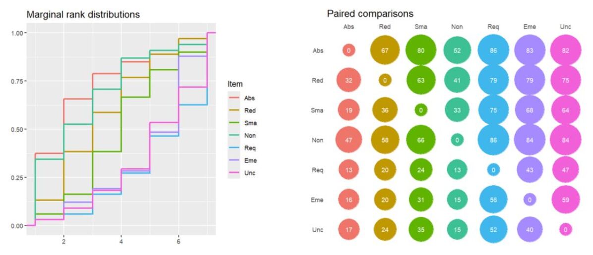
Figure 1: Ecdf’s of the marginal rank distributions (left) and bubble plot of the pairwise comparison matrix (right) for the Antifragility dataset.

Concerning ranking data manipulation, MSmix provides functions designed to switch from complete to partial sequences, with the routine data_censoring, or from partial to complete sequences, with the routines data_augmentation and data_completion. These functions are particularly useful in simulation scenarios for evaluating the robustness of inferential procedures in recovering the actual data-generating mechanisms under various types and extents of censoring and different data augmentation strategies for handling partial data.

With data_censoring, the truncation of complete rankings can be either applied with the top-$k$ scheme, or the missing at random (MAR) procedure. To retain the information on the top positions, the user needs to set the argument type = "topk"; instead, to retain information on a random set of positions, she needs to set the argument type = "mar". Regardless of the censoring process type, the user can choose the number of positions to be retained for each ranked sequence in: (i) a deterministic way, by specifying an integer vector in the nranked argument, indicating the desired length of each partial sequence; (ii) a stochastic way, by setting nranked = NULL (default) and providing in the argument probs the probabilities for the random number of positions to be kept after censoring, that is, for 1, 2, up to $(n-1)$ ranks. An example of a deterministic top-$k$ censoring scheme is implemented below to covert the complete Antifragility ranking data into top-3 rankings. R> N <- nrow(ranks_AF) R> top3_AF <- data_censoring(rankings = ranks_AF, type = "topk", + nranked = rep(3,N)) R> top3_AF$part_{r}ankings[1:3,]\CodeChunk\CodeOutput AbsRedSmaNonReqEmeUnc1NA213NANANA21NA32NANANA33NA12NANANATheoutputof\code{data_{c}ensoring}isalistwithafirstcomponent,named\code{part_{r}ankings},correspondingtotheinputcompletedatamatrix\code{rankings}withsuitablycensored(\code{NA})entries,andasecondcomponent,named\code{nranked},correspondingtothevectorwiththenumberofactuallyvisiblepositionsineachpartialranking.\par Anexampleofstochastictop-$k$censoringschemeonthesamedataset,thatwillresultinarandomnumberofbottompositionsobscured,canberunasfollows\CodeChunk\CodeInput R>top_{A}F<-data_{c}ensoring(rankings=ranks_{A}F,type="topk",+probs=c(1:(n-2),0))R>top_{A}F$part_{r}ankings[1:3,]\CodeChunk\CodeOutput AbsRedSmaNonReqEmeUnc142135NANA21NA32NANANA33NA12NANANA\CodeChunk\CodeInput R>table(top_{A}F$nranked)\CodeChunk\CodeOutput 12345114161949Inthiscase,theprobabilityvector\code{probs}isassigninganincreasingchanceofretainingahighernumberoftoppositions,withtheexceptionofazerovalueinthelastentry,forcingthenon-occurrenceoffullrankingsaftercensoring.Apartfromthedifferentsettingforthe\code{type}argument,applyingaMARcensoringschemerequiresasimilarsyntaxtothetop-$k$.Themaindifferenceisthat,insteadofthecensoringprocessactingonlyonthebottompartoftherankings,thepositionstobecensoredaredetermineduniformlyatrandomoncethenumberofrankstobekeptisspecifiedbytheuser(eitherdeterministicallyorstochastically).\par Weconcludethissectionwithanillustrationofthecounterpartcommandsof\code{data_{c}ensoring}in\pkg{MSmix},whichactonpartialrankingsandfillinthemissingpositionswithdifferentcriteria.Thefirst,called\code{data_{a}ugmentation},isthekeyfunctionforestimatingMMS-mixonpartialrankingsviaAlgorithm\ref{alg:partial_mixture}.Hereisatoyexamplewithonlytwopartialrankingscharacterizedbydifferenttypesofcensoring,respectivelyatop-3andaMARsequence\CodeChunk\CodeInput R>ranks_{t}oy<-rbind(c(2,NA,1,NA,3),c(NA,4,NA,1,NA))R>ranks_{t}oy\CodeOutput[,1][,2][,3][,4][,5][1,]2NA1NA3[2,]NA4NA1NA\CodeInput R>data_{a}ugmentation(rankings=ranks_{t}oy)\CodeOutput[[1]][,1][,2][,3][,4][,5][1,]24153[2,]25143\par[[2]][,1][,2][,3][,4][,5][1,]24315[2,]34215[3,]34512[4,]24513[5,]54213[6,]54312Theoutputlistcontainsthematricesofallpossiblefullrankingscompatiblewitheachpartialsequence.Weremarkthat,despitethename\code{rankings}oftheinputpartiallyrankeddatamatrix,thisfunctioncanalsobeappliedtopartialobservationsexpressedinorderingformat.Ingeneral,itsupportsthedataaugmentationofsequencescontainingatmost10missingentries.\par Thesecondfunction,named\code{data_{c}ompletion},completespartialrankingswithasinglefullranking.Tocompletetherankingsin\code{ranks_{t}oy},oneneedstospecifythe\code{ref_{r}ho}argumentwithamatrixofthesamedimensionsas\code{ranks_{t}oy},containingthereferencefullrankingsineachrow.Intheexamplebelow,weusetheidentitypermutationanditsoppositeasthereferencesequencesforcompletion.\CodeChunk\CodeInput R>data_{c}ompletion(rankings=ranks_{t}oy,ref_{r}ho=rbind(1:5,5:1))\CodeChunk\CodeOutput[,1][,2][,3][,4][,5][1,]24153[2,]54312Theoutputisthematrixobtainedbyfillinginthemissingentriesofeachpartialsequencewiththerelativepositionsoftheunrankeditemsaccordingtothereferencefullranking.\code{data_{c}ompletion}accommodatesanytypeofcensoring,similarto\code{data_{a}ugmentation},butwithouttheneedtoenumerateallpossibleordersofmissingpositions.Consequently,thereisnoupperlimitonthenumberof\code{NA}entriesinthepartialsequences.\par$

4.3 Sampling

The function devoted to simulating an i.i.d. sample of full rankings from a MMS-mix is rMSmix, which relies on the Metropolis-Hastings (MH) procedure implemented in the R package BayesMallows (BayesMallows). When $n\leq 10$, we also offer the possibility to perform exact sampling. This can be achieved by setting the logical mh argument to FALSE.

The rMSmix function requires the user to specify: i) the desired number of permutations (sample_size), ii) the number of items (n_items) and iii) the number of mixture components (n_clust). The mixture parameters can be passed with the separated (and optional) arguments rho, theta and weights, set to NULL by default. If the user does not input the above parameters, the concentrations are sampled uniformly in the interval $(1/n^{2},3/n^{3/2})$, while the simulation of the consensus parameters and the weights can be selected with the logical argument uniform. The option uniform = TRUE consists in generating the non-specified parameters uniformly in their support. Here is an example where $N=100$ full rankings of $n=8$ items are exactly generated from a $3-$component MMS-mix, with assigned and equal concentrations $\bm{\theta}=(.15,.15,.15)$ and the other parameters sampled uniformly at random. R> theta = rep(.15, 3) R> sam <- rMSmix(sample_size = 100, n_items = 8, n_clust = 3, theta = theta, + uniform = TRUE, mh = FALSE)

The function rMSmix returns a list of five named objects: the $N\times n$ matrix with the simulated complete rankings (samples), the model parameters actually used for the simulation (rho, theta and weights) and the simulated group membership labels (classification).

For the previous example, they can be extracted as follows R> sam$samples[1:3,]\par[,1][,2][,3][,4][,5][,6][,7][,8][1,]61758324[2,]21375486[3,]62758314\par R>sam$rho

[,1] [,2] [,3] [,4] [,5] [,6] [,7] [,8] [1,] 6 2 1 5 4 3 8 7 [2,] 4 2 5 3 8 7 1 6 [3,] 6 2 8 4 7 3 1 5

R> sam$weights\par[1]0.491655350.041236270.46710838\par R>table(sam$classification)

1 2 3 35 5 60 One can note that, with uniform sampling, cluster separation and balance of the drawings among the mixture components are not guaranteed. In fact, cluster 2 has a very small weight ($\omega_{2}\approx 0.04$) corresponding to only 5 observations; moreover, the consensus rankings of clusters 2 and 3 are quite similar, as testified by their low relative Spearman distance. R> max_spear_dist <- 2*choose(8+1,3) R> spear_dist(rankings = sam$rho[2,],rho=sam$rho[3,])/max_spear_dist [1] 0.1904762

To ensure separation among the mixture components and non-sparse weights, the user can set the option uniform = FALSE. Specifically, the consensus rankings are drawn with a minimum Spearman distance from each other equal to $\frac{2}{G}\binom{n+1}{3}$, and the mixing weights are sampled from a symmetric Dirichlet distribution with (large) shape parameters $\bm{\alpha}=(2G,\dots,2G)$ to favour populated and balanced clusters. R> sam <- rMSmix(sample_size = 100, n_items = 8, n_clust = 3, theta = theta, + uniform = FALSE, mh = FALSE)

We notice that now the three clusters are more balanced, and with central rankings at larger relative distance.

R> sam$weights\CodeOutput[1]0.52144950.25947820.2190723\CodeInput R>spear_{d}ist(rankings=sam$rho)/max_{s}pear_{d}ist\CodeOutput 1220.630952430.70238100.6666667\par InFigure\ref{fig:s1}weshowtheseparationamongclustersinthetwoexamplesthroughtheSpearmandistancematrixofthesimulatedsamples,whichquantifiesthedissimilaritybetweeneachpairofobservations.Forexample,Figure\ref{fig:s1b}canbeconstructedasfollows\CodeChunk\CodeInput R>plot.dist(spear_{d}ist(rankings=sam$samples))\par Itsuggeststhepresenceofonlytwowell-separatedclustersinthesample,whilethreeclustersareevidentfromFigure\ref{fig:s1b}.\par\begin{figure}[t]\centering\begin{subfigure}[b]{212.47617pt}\centering\includegraphics[width=433.62pt]{dist1.pdf}\@@toccaption{{\lx@tag[ ]{{(a)}}{Uniformlysampledparameters.}}}\@@caption{{\lx@tag[ ]{{\small(a)}}{\small Uniformlysampledparameters.}}}\@add@centering\end{subfigure}\hfill\begin{subfigure}[b]{212.47617pt}\centering\includegraphics[width=433.62pt]{dist2.pdf}\@@toccaption{{\lx@tag[ ]{{(b)}}{Separatedclusters.}}}\@@caption{{\lx@tag[ ]{{\small(b)}}{\small Separatedclusters.}}}\@add@centering\end{subfigure}\@@toccaption{{\lx@tag[ ]{{2}}{AvisualizationoftherandomdrawsfromaMMS-mix,obtainedbysetting\code{uniform=TRUE}(a),and\code{uniform=FALSE}(b).}}}\@@caption{{\lx@tag[: ]{{\small Figure 2}}{\small AvisualizationoftherandomdrawsfromaMMS-mix,obtainedbysetting\code{uniform=TRUE}(a),and\code{uniform=FALSE}(b).}}}\@add@centering\end{figure}\par\par Inconclusion,\code{rMSmix}isdesignedtofacilitatetheimplementationofalternativesamplingschemes,thatcanbefruitfultoassesstheperformanceoftheinferentialproceduresandtheirrobustnessunderavarietyofsimulationscenarios.\par\par$

4.4 Application on full rankings

In this section, we show how to perform a mixture model analysis on the Antifragility rankings. To this aim, we use the command fitMSmix, the core function of the MSmix package, which performs MLE of the MMS-mix on the input rankings via EM algorithm with the desired number n_clust of components. The number of multiple starting points, needed to address the issue of local maxima, can be set through the argument n_start, and the list init possibly allows to configure initial values of the parameters for each starting point.

We now estimate several MMS-mix with a number of components ranging from 1 to 6 and save the BIC (Bayesian informative criterion) values in a separate vector for then choosing the optimal number of clusters. R> FIT.try <- list() R> BIC <- setNames(numeric(6), paste0(’G = ’, 1:6)) R> for(i in 1:6) + FIT.try[[i]] <- fitMSmix(rankings = ranks_AF, n_clust = i, n_start = 50) + BIC[i] <- FIT.try[[i]]$mod$bic The BIC values of the six estimated models are R> print(BIC) G = 1 G = 2 G = 3 G = 4 G = 5 G = 6 1494.435 1461.494 1442.749 1444.223 1449.714 1453.101

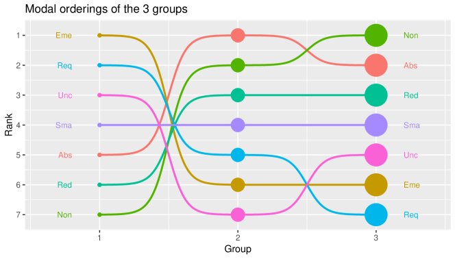
Figure 3: Bump plot depicting the estimated consensus rankings of the three clusters for the ranks_antifragility dataset, obtained with the generic function plot.emMSmix.

suggesting G = 3 as the optimal number of groups (lowest BIC). The function fitMSmix creates an object of S3 class "emMSmix", which is a list whose main component, named mod, describes the best fitted model over the n_start initializations. It includes, for example, the MLE of the parameters (rho, theta and weights), fitting measures (log_lik and bic), the estimated posterior membership probabilities (z_hat) and the related MAP allocation (map_classification) as well as the indicator of convergence achievement (conv).

The MLEs of the best fitted model can be shown also through the summary.emMSmix method, R> summary(object = FIT.try[[3]]) Call: fitMSmix(rankings = ranks_AF, n_clust = 3, n_start = 50)

—————————– — MLE of the parameters — —————————–

Component-specific consensus rankings: Abs Red Sma Non Req Eme Unc Group1 5 6 4 7 2 1 3 Group2 1 3 4 2 5 6 7 Group3 2 3 4 1 7 6 5

Component-specific consensus orderings: Rank1 Rank2 Rank3 Rank4 Rank5 Rank6 Rank7 Group1 "Eme" "Req" "Unc" "Sma" "Abs" "Red" "Non" Group2 "Abs" "Non" "Red" "Sma" "Req" "Eme" "Unc" Group3 "Non" "Abs" "Red" "Sma" "Unc" "Eme" "Req"

Component-specific precisions: Group1 Group2 Group3 0.111 0.241 0.087

Mixture weights: Group1 Group2 Group3 0.083 0.343 0.574 which also displays the estimated modal orderings. The generic function plot.emMSmix is also associated to the class "emMSmix" and constructs two fancy plots. The first one is the bump plot (Figure 3) depicting the consensus ranking of each cluster, with different colors assigned to each item, circle sizes proportional to the estimated weights and lines to better highlight item positions in the modal orderings of the various components. For this example, we note that the size of the second cluster is almost half that of the third cluster, while the first cluster is very small. Moreover, the two larger groups (2 and 3) exhibit very similar modal rankings and quite opposite preferences with respect to the first cluster (items such as “Emergence”, “Requisite variety”, and “Uncoupling” are ranked at the top in cluster 1, but placed at the bottom in groups 2 and 3).

Figure 4 shows, instead, the individual cluster memberships probabilities, describing the uncertainty with which each observation could be assigned to the mixture components. For example, the units 10, 15, 19, 20, 71, 74, 78 and 94 have high probabilities (close to 1) of belonging to group 1. Instead, some units (e.g., unit 8, 28, 36, and 44) have similar membership probabilities of belonging to clusters 2 or 3, indicating less confidence in their assignment to one of the two groups. On the other hand, when some clusters are close on the ranking space, a certain degree of uncertainty in recovering the true membership is expected.

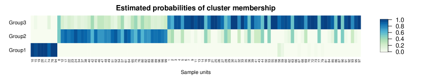
Figure 4: Heatplot of the estimated probabilities of cluster memberships for each observation of the ranks_antifragility dataset, obtained with the generic function plot.emMSmix.

The package provides also routines for CI computation, working with the object of class "emMSmix" as first input argument. For example, we can produce Hessian-based CIs for the precisions and mixture weights with confintMSmix, which is a function specific for full ranking data. With the default confedence level (conf_level = 0.95), one obtains

R> confintMSmix(object = FIT.try[[3]]) Hessian-based 95

lower upper Group1 0.055 0.168 Group2 0.186 0.296 Group3 0.069 0.105

Hessian-based 95

lower upper Group1 0.064 0.101 Group2 0.328 0.359 Group3 0.560 0.588

Another possibility relies on bootstrap CI calculation. Let us opt for the soft bootstrap method (the default choice when $G>1$) which, unlike the separated one (type = "separated"), produces CIs also for weights. We require n_boot = 500 bootstrap samples and then print the output object of class "bootMSmix" through the generic function print.bootMSmix.

R> CI_bootSoft <- bootstrapMSmix(object = FIT.try[[3]], n_boot = 500, all = TRUE) R> print(CI_bootSoft) Bootstrap itemwise 95

Abs Red Sma Non Req Eme Group1 "3,4,5,6,7" "4,5,6,7" "2,3,4,5,6" "6,7" "1,2,3,4" "1,2" Group2 "1" "2,3" "4" "2,3" "5" "6" Group3 "1,2,3" "2,3" "4,5" "1,2" "7" "5,6" Unc Group1 "2,3,4,5" Group2 "7" Group3 "4,5,6"

Bootstrap 95

lower upper Group1 0.068 0.212 Group2 0.193 0.314 Group3 0.069 0.112

Bootstrap 95

lower upper Group1 0.071 0.101 Group2 0.283 0.404 Group3 0.505 0.636 The bootstrap itemwise intervals for the consensus ranking are wider in the first group, the smallest one, while the second cluster shows very little uncertainty. Note also that the Hessian-based intervals for the precisions and the weights are narrower than the bootstrap ones, except for the weight of the first cluster that has a few observations.

The logical argument all indicates whether the MLEs estimates obtained from the bootstrap samples must be returned in the output. When all = TRUE, as in this case, the user can visualize the bootstrap sample variability with the generic function plot.bootMSmix. It returns the heatmap of the first-order marginals of the bootstrap samples (an example is available in Figure LABEL:fig:heat_beers), and kernel densities for the precisions and weights (Figure 5).

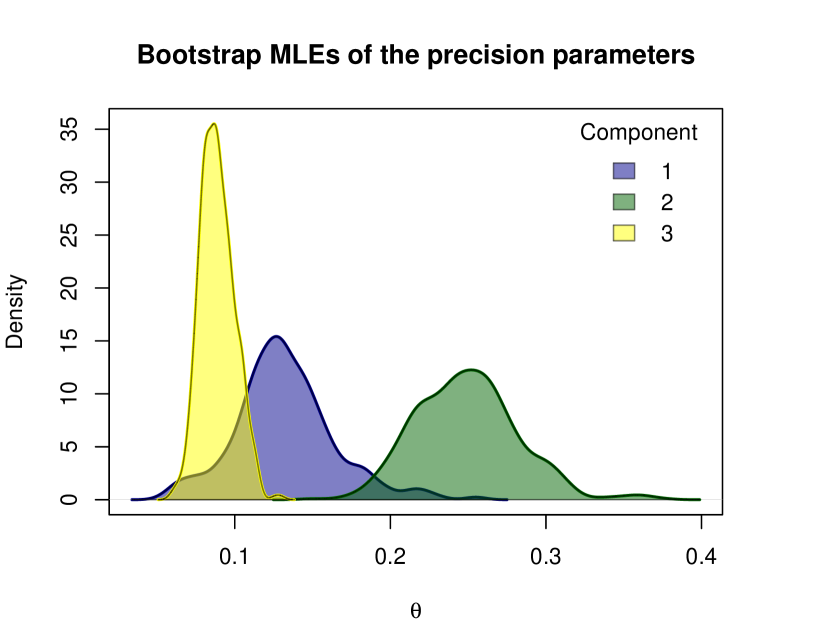
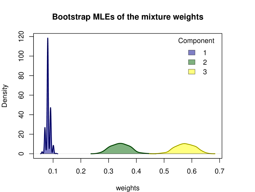
Figure 5: Kernel densities of the soft bootstrap MLEs of the precision parameters (left) and weights (right) for the ranks_antifragility dataset.

4.5 Application on partial rankings

In this section we illustrate how to perform inference on the MAR partial rankings by exploiting the original ranks_beers dataset. These data were collected through an online survey administered to the participants of the 2018 Pint of Science festival held in Grenoble. A sample of $N=105$ subjects provided their partial rankings of $n=20$ beers according to their personal tastes. The rankings are recorded in the first 20 columns of the dataset, while column 21 contains a covariate regarding respondents’ residency.

The barplot with the percentages of the number of beers actually ranked by the participants is reported in Figure 6. We restrict the analysis to partial rankings with maximum 8 missing positions, to show both the data augmentation schemes (Algorithms 3 and 4) implemented in the package. Thanks to the subset argument of fitMSmix, we can specify the subsample of observations to be considered directly in the fit command. To speed up the estimation process, we parallelize the multiple starting points by setting parallel = TRUE.

R> rankings <- ranks_beers[,1:20] R> subset_beers <- (rowSums(is.na(rankings)) <= 8) R> library(doParallel) R> registerDoParallel(cores = detectCores()) R> FIT_aug <- fitMSmix(rankings,n_clust = 1, n_start = 15, + subset = subset_beers, mc_em = FALSE, parallel = TRUE) R> FIT_mcem <- fitMSmix(rankings, n_clust = 1, n_start = 15, + subset = subset_beers, mc_em = TRUE, parallel = TRUE)

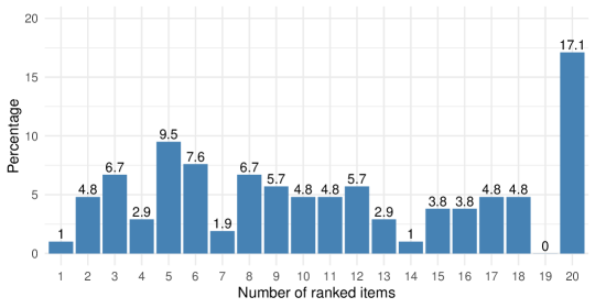
Figure 6: Percentages of the number of ranked items in the ranks_beers dataset. This barplot was obtained as first plot in the output of the data_description routine.

The logical mc_em argument indicates whether the MCEM scheme (Algorithm 4) must be applied. When mc_em = FALSE (default), Algorithm 3 is implemented.

We note that, for this application, the results of the two methods are very similar.

R> spear_dist(FIT_aug$mod$rho,FIT