Non-Abelian spin Hall insulator

Abstract

Motivated by a recent experiment reporting the fractional quantum spin Hall effect in twisted ${\rm MoTe}_{2}$, we investigate microscopically the prospects of realizing exotic topologically ordered states beyond conventional quantum Hall physics. We show that a non-Abelian spin Hall insulator, a state of two copies of the non-Abelian Moore-Read state, can be stabilized at half filling of time-reversal conjugate Chern bands. We elucidate that the existence of this phase relies on the reduction of opposite-spin interactions at short distances to overcome the Ising ferromagnetism. Moreover, we demonstrate that band mixing provides a generic mechanism for this reduction to be achieved. Quite remarkably, we find that a renormalization of opposite-spin interactions at short distances as small as 15 % of the moiré period is sufficient for a direct transition to a completely spin unpolarized phase which supports the non-Abelian spin Hall insulator. Furthermore, we show that the non-Abelian spin Hall insulator can either break time-reversal symmetry or preserve it depending on the underlying topological order.

I I. Introduction

Electron fractionalization is a central theme of modern condensed matter physics. About four decades ago, the study of the fractional quantum Hall effect of two-dimensional electron systems under high magnetic field revealed the existence of quasiparticles in a partially filled Landau level which carry fractional charge and obey fractional statistics Tsui et al. (1982); Laughlin (1983). Recently, fractional quantum anomalous Hall states were discovered in two-dimensional semiconductor and graphene moiré systems at zero magnetic field Zeng et al. (2023); Cai et al. (2023); Park et al. (2023); Xu et al. (2023); Lu et al. (2024). In both cases, the emergence of fractional quasiparticle requires breaking time-reversal symmetry due to external magnetic field or spontaneous ferromagnetism Li et al. (2021); Crépel and Fu (2023), and is marked by the fractionally quantized Hall conductance. On the other hand, as the vast majority of quantum materials are nonmagnetic, there is growing interest in the possibility of electron fractionalization with time reversal symmetry Levin and Stern (2009); Neupert et al. (2011); Freedman et al. (2004); Repellin et al. (2014); Bernevig and Zhang (2006).

Topological quantum materials with time-reversed pairs of Chern bands Kane and Mele (2005), such as twisted homobilayer MoTe₂ and WSe₂ Wu et al. (2019); Devakul et al. (2021), provide a promising venue for fractional electron states. While most studies have focused on fractional Chern insulators in which spontaneously spin-polarized electrons populate a single Chern band Cai et al. (2023); Park et al. (2023); Zeng et al. (2023); Xu et al. (2023), a recent transport experiment Kang et al. (2024a) has reported an incompressible state in twisted $\text{MoTe}_{2}$ at odd-integer hole filling $\nu=3$, which has vanishing Hall conductivity accompanied by fractional edge conductance $\frac{3}{2}e^{2}/\hbar$. This sharply contrasts with the quantum anomalous Hall (QAH) state at $\nu=1$ with complete filling of a single Chern band Devakul et al. (2021); Foutty et al. (2024), or the (double) quantum spin Hall states at $\nu=2$ or $4$ with complete filling of time-reversed pairs of Chern bands Devakul et al. (2021); Wu et al. (2019); Kang et al. (2024b).

The observed $\nu=3$ state has attracted great interest. A number of time-reversal-invariant and time-reversal-breaking phases with different fractional excitations has been proposed on phenomenological grounds May-Mann et al. (2024); Jian and Xu (2024); Villadiego (2024); Zhang (2024); Chou and Sarma (2024). However, no microscopic calculation has been performed to shine light on the likely ground states of twisted semiconductor bilayers at $\nu=3$.

In this work, we identify two competing strong-coupling phases at $\nu=3$, a quantum anomalous Hall insulator and a non-Abelian spin Hall insulator. We demonstrate that the competition between the two phases is governed by the behavior of electron-electron interactions at short distances which we systematically investigate. In addition, we establish band mixing as a microscopic mechanism for controlling the effective interaction at short distance and therefore the competition between the two phases.

Our results are obtained through a microscopic model study of interacting electron systems featuring time-reversed pairs of narrow Chern bands with $C_{\uparrow}=-C_{\downarrow}=1$ at odd-integer band fillings $\nu\equiv\nu_{\uparrow}+\nu_{\downarrow}=1\mod 2$. In the flat band limit, if the gap to higher bands is large so that band mixing can be neglected, Coulomb interaction drives the system into a fully spin-polarized QAH state. However, we find that a reduction of the short-range part of Coulomb repulsion between two opposite-spin electrons can result in a spin unpolarized state with both $C_{\uparrow}=1$ and $C_{\downarrow}=-1$ bands at equal half-integer filling.

We further show that if the underlying Chern band wavefunctions mimics that of the $n=1$ Landau level Reddy et al. (2024), the spin unpolarized ground state is a non-Abelian spin Hall insulator, which is adiabatically connected to the product of two non-abelian Moore-Read states Moore and Read (1991); Read and Green (2000) in conjugate Chern bands. This state has vanishing electrical Hall conductivity, quantized spin Hall conductivity $\sigma^{sh}=\frac{3}{2}$, and supports both charge $e/4$ non-Abelian Ising anyons and $e/2$ Abelian anyons in the bulk. Interestingly, two types of non-Abelian spin Hall insulators are identified: a time-reversal-invariant phase (a non-Abelian topological insulator), and a time-reversal-breaking phase that exhibits quantized thermal Hall conductance $\kappa_{H}=\pm 2$. Remarkably, our non-Abelian state only requires a small renormalization of Coulomb interaction at short distance (which can be as small as $15\%$ of the moiré period), and can already emerge at a moderate amount of band mixing.

Our work is organized as follows. We start by introducing a minimal model that captures the essential feature of conjugate Chern bands in twisted TMD bilayers (section II). Since spin $\uparrow$ and $\downarrow$ particles belong to conjugate Chern bands of opposite chirality, our system lacks spin $SU(2)$ symmetry and its energy spectrum depends crucially on the total spin (section III).

Next, we show rigorously that in the absence of band mixing, the ground state of our model at odd integer fillings is necessarily fully spin polarized if the bare interaction is spin independent and repulsive (section IV). However, when opposite-spin repulsion is reduced at short distance, we find by analytical calculations that the ferromagnetic state can become unstable to a single spin flip (section V).

This motivates us to study the ground state phase diagram by many-body exact diagonalization calculation (section VI). Remarkably, as the opposite-spin repulsion is reduced, the fully polarized state transitions directly into an unpolarized state. The latter has an approximate ground state degeneracy of $6\times 6$ and $2\times 2$ for even and odd number of particles respectively, as expected for the product of two Moore-Read states in opposite magnetic fields. Two types of “doubled” Moore-Read phases are discussed, which are time-reversal-invariant and spontaneous time-reversal-breaking respectively (section VII).

Moreover, we show quantitatively that the reduction of opposite-spin interaction at short distance naturally arises from the band mixing effect (section VIII).

Finally, we discuss the relevance of our finding for the observed $\nu=3$ state in twisted MoTe₂ (section IX) and outline future directions (section X).

II II. Model

Our work is motivated by the physics of twisted transition metal dichalcogenide homobilayers ($t$TMDs) such as $t$MoTe₂, described by the following Hamiltonian:

$$\begin{gathered}H=\int d^{2}r\psi_{\sigma}^{\dagger}(\mathbf{r})\mathcal{H}_{\sigma}\psi_{\sigma}(\mathbf{r})+H_{\rm int}\end{gathered}$$ (1)

where $\psi_{\sigma}^{\dagger}(\mathbf{r})$ with $\sigma=\pm$ creates a spin $s_{z}=\uparrow$ or $\downarrow$ particle (which corresponds to a hole excitation in the valence band). $\mathcal{H}$ describes the non-interacting band structure of a single hole. Due to strong Ising spin-orbit coupling, our system only has spin $U(1)$ symmetry, and spin $\uparrow$ and $\downarrow$ bands form time-reversed pairs, satisfying $\mathcal{H}_{+}=\mathcal{H}^{*}_{-}$. The second term $H_{\rm int}$ describes the interaction between holes which we will specify later.

The key feature of $t$TMDs is time-reversed pairs of topological moiré bands, which carry a spin-dependent Chern number $C_{\uparrow}=-C_{\downarrow}=1$ Wu et al. (2019). These Chern bands are formed by a real-space topological texture of “Zeeman” field acting on the layer pseudospin degree of freedom. When the Zeeman field is large, the pseudospin is locally aligned to the Zeeman field, giving rise to an effective Hamiltonian description of the low-energy band structure Paul et al. (2022); Morales-Durán et al. (2024),

$$\mathcal{H}_{\sigma}=\frac{(\mathbf{p}+\sigma e\mathbf{A}(\mathbf{r}))^{2}}{2m}+V(\mathbf{r}).$$ (2)

Here, $\mathbf{A}(\mathbf{r})$ is a $U(1)$ gauge field that represents an emergent magnetic field $B(\mathbf{r})$ with one flux quanta per moiré unit cell, while $V(\mathbf{r})$ is a scalar potential. Due to time-reversal symmetry, opposite spins feel opposite magnetic fields and identical scalar potential. Both $B(\mathbf{r})$ and $V(\mathbf{r})$ are periodically varying with the periodicity of the moiré superlattice. The Hamiltonian (2), which describes a charged particle subject to a periodic magnetic field and a periodic potential, defines the adiabatic model of twisted TMDs.

It is instructive to first study the simplified version of the Hamiltonian (2), where we only keep the uniform component of the emergent magnetic field, neglecting other Fourier components of $B(\mathbf{r})$ and $V(\mathbf{r})$ at nonzero reciprocal lattice vectors. In this approximation—which turns out to be accurate near a magic twist angle Morales-Durán et al. (2024); Reddy et al. (2024), the moiré bands of our system are simply conjugate pairs of Landau levels with opposite spins (LLs), produced by equal and opposite magnetic fields and related by time-reversal symmetry. We label the time-reversed pair of LLs as ($n$LL, $n\overline{\rm LL}$) with $n=0,1,...$ the Landau level index.

When the band gap is large enough that the effect of band mixing can be neglected, at total band filling $\nu=2n+1$, the lowest $n$ LL pairs are completely filled and inert, while interacting fermions in the next LL pair (corresponding to LL index $n$) at effective filling $\nu_{\uparrow}+\nu_{\downarrow}=1$ is described by the Hamiltonian

$$\begin{split}\tilde{H}=\frac{1}{2S_{M}}\sum_{\mathbf{q}\sigma}V_{n}(\mathbf{q}):\rho_{\sigma}(\mathbf{q})\rho_{\sigma}(-\mathbf{q}):\\ \>\>\>\>\>\>\>+U_{n}(\mathbf{q}):\rho_{\sigma}(\mathbf{q})\rho_{-\sigma}(-\mathbf{q}):\end{split}$$ (3)

where $\rho_{\sigma}(\mathbf{q})$ is the projected density operator for spin $\sigma$ given by $\rho_{\sigma}(\mathbf{q})=\sum_{\mathbf{k}}\langle\mathbf{k}+\mathbf{q}|e^{i\mathbf{q}\cdot\mathbf{R}^{\sigma}}|\mathbf{k}\rangle c^{\dagger}_{\mathbf{k}+\mathbf{q}\sigma}c_{\mathbf{k}\sigma}$ with $\mathbf{R}^{\sigma}$ the guiding center coordinate sup . $S_{M}$ is the area of the moiré system and $::$ denotes normal ordering.

The density operators of equal spin satisfy the spin-dependent GMP algebra Girvin et al. (1986),

$$[\rho_{\sigma}(\mathbf{q}_{1}),\rho_{\sigma}(\mathbf{q}_{2})] = 2i\sigma\sin(l^{2}_{B}\mathbf{q}_{1}\wedge\mathbf{q}_{2})\rho_{\sigma}(\mathbf{q}_{1}+\mathbf{q}_{2})$$ (4)

where $l_{B}$ is the magnetic length set by one emergent flux quanta per moiré unit cell, $2\pi l^{2}_{B}=\frac{\sqrt{3}}{2}a_{M}^{2}$ with $a_{M}$ the moiré period. It is important to note that the commutators for spin-$\uparrow$ and $\downarrow$ take opposite signs, reflecting the opposite chirality of the corresponding LLs. The density operators of different spins commute:

$$[\rho_{+}(\mathbf{q}_{1}),\rho_{-}(\mathbf{q}_{2})]=0.$$ (5)

The band-projected Hamiltonian (3) defines a concrete model we shall study below.

In the absence of moiré band mixing, $V_{n}(\mathbf{q})$ and $U_{n}(\mathbf{q})$ are obtained from the interaction between two equal- and opposite-spin particles projected onto ($n$LL, $n\overline{\rm LL}$). For the bare Coulomb interaction $V(\mathbf{r})=e^{2}/(\epsilon\>\mathbf{r})$, we find

$$V_{n}(\mathbf{q})=\left(\frac{2\pi e^{2}}{\epsilon|\mathbf{q}|}\right)e^{-|\mathbf{q}|^{2}l^{2}_{B}/2}[L_{n}(|\mathbf{q}|^{2}l_{B}^{2}/2)]^{2}$$ (6)

where $L_{n}$ is the $n$-th Laguerre polynomial, and $U_{n}(\mathbf{q})=V_{n}(\mathbf{q})$ due to the time reversal relation between conjugate LLs. While the long-range part of electron-electron interaction described by Coulomb’s law is indeed spin independent, the interaction at short distance is generally spin-dependent, especially considering the strong atomic spin-orbit coupling in TMD. Moreover, as we shall show explicitly later, moiré band mixing will strongly reduce the opposite-spin interaction $U_{n}$ compared to the equal-spin interaction $V_{n}$.

Keeping these considerations in mind, in this work we consider projected interactions on a pair of conjugate Chern bands that are spin dependent. In particular, we find it useful to consider interactions in the $n$-th pair of conjugate LLs of the form:

$$U_{n}(\mathbf{q})=e^{-d|\mathbf{q}|}V_{n}(\mathbf{q})$$ (7)

where $d$ is a spin anisotropy parameter. It is important to note that the introduction of $d$ mainly affects the short distance behavior of the projected interaction between opposite-spin particles, while at long distance ($\mathbf{q}\rightarrow 0$), $U_{n}$ and $V_{n}$ converge to the same value as physically required.

The interactions defined in (6) and (7) have a physically transparent meaning. At small $d$, $U_{n}$ can be rewritten as $U_{n}=V_{n}+\delta U_{n}$ with the correction $\delta U_{n}$ given by

$$\delta U_{n} = -(1-e^{-d|\mathbf{q}|})V_{n}(\mathbf{q})$$ (8)

$$\approx -\left(\frac{2\pi e^{2}d}{\epsilon}\right)e^{-|\mathbf{q}|^{2}l^{2}_{B}/2}[L_{n}(|\mathbf{q}|^{2}l_{B}^{2}/2)]^{2}.$$

This corresponds to a delta-function attraction between opposite spins projected onto the $n$-th conjugate LLs, added to the spin-independent Coulomb interaction. In other words, the role of small $d$ is to reduce the electron-electron interaction between two opposite-spin particles at short distances from the Coulomb case while the overall interaction remains repulsive at all distances. In the opposite limit $d\rightarrow\infty$, spin-$\uparrow$ and $\downarrow$ particles are essentially decoupled, which will greatly aid our analysis below.

III III. Two-Body Energy Spectrum

The interaction $V_{n}$ between two particles of equal spin in the $n$-th LL is familiar in the quantum Hall literature. Assuming full rotational invariance, it can be naturally decomposed into the standard Haldane pseudopotentials Haldane (1983) of the $n$-th LL denoted as $V_{n}^{m}$ with $m$ the relative angular momentum,

$$V_{n}^{m}=\int\dfrac{d^{2}\mathbf{q}}{(2\pi)^{2}}V(\mathbf{q})[L_{n}(|\mathbf{q}|^{2}l^{2}_{B}/2)]^{2}L_{m}(|\mathbf{q}|^{2}l^{2}_{B})e^{-|\mathbf{q}|^{2}l^{2}_{B}}$$ (9)

On the other hand, $U_{n}$ describes the interaction between two particles of opposite spin in conjugate LLs, which doesn’t allow for a similar decomposition. Nonetheless, the two-body problem of $U_{n}$ can still be solved Stefanidis and Sodemann (2020) due to the algebra of guiding center relative coordinates, $\mathbf{R}^{\rm rel}=\mathbf{R}^{\uparrow}_{1}-\mathbf{R}^{\downarrow}_{2}$ which obeys

$$[\mathbf{R}^{\rm rel}_{a},\mathbf{R}^{\rm rel}_{b}]=0$$ (10)

for $a,b=x,y$ sup . The two-body energy spectrum can then be labelled by $\mathbf{R}^{\rm rel}$ and are given by

$$U_{n}({\mathbf{R}^{\rm rel}})=\int\frac{d^{2}\mathbf{q}}{(2\pi)^{2}}U_{n}(\mathbf{q})e^{i\mathbf{q}\cdot\mathbf{R}^{\rm rel}}$$ (11)

The highest energy state corresponds to a bound state of two particles with a vanishing separation $\mathbf{R}^{\rm rel}=0$, which has the largest repulsion energy $U_{n}(0)$.

In addition, since two particles of opposite spin interacting by $U_{n}$ feel opposite magnetic fields, they drift parallel to each other with total momentum perpendicular to their separation, $\mathbf{K}=-\hat{z}\crossproduct\mathbf{R}^{\rm rel}/l^{2}_{B}$ in an analogous manner to neutral excitons in Landau levels Gor’kov and Dzyaloshinskii (1968); Kallin and Halperin (1984), leading to a dispersive band of two-body excitations with total spin $S_{z}=0$.

We now focus on the $n=1$ LL, the equal-spin pseudopotentials $V_{1}^{m}$ read

$$V_{1}^{m}=\frac{e^{2}}{\epsilon l_{B}}\dfrac{\Gamma(m+1/2)}{2m!}\dfrac{(m-3/8)(m-11/8)}{(m-1/2)(m-3/2)}$$ (12)

and the largest repulsion energy for opposite-spin interactions is given by

$$U_{1}(0)=\dfrac{e^{2}}{\epsilon l_{B}}\dfrac{1}{8}\big{[}-2\big{(}\frac{d}{l_{B}}+\frac{d^{3}}{l_{B}^{3}}\big{)}+\big{(}3+2\frac{d^{2}}{l_{B}^{2}}+\frac{d^{4}}{l_{B}^{4}}\big{)}e^{d^{2}/2l_{B}^{2}}\sqrt{2\pi}{\rm erfc}(\dfrac{d}{\sqrt{2}l_{B}})\big{]}$$ (13)

For later discussions, we define $\eta=U_{1}(0)/\frac{3}{4}\frac{e^{2}}{\epsilon l_{B}}\sqrt{\frac{\pi}{2}}$ to be the ratio of the largest opposite-spin repulsion energy at any $d$ to its value when $d=0$.

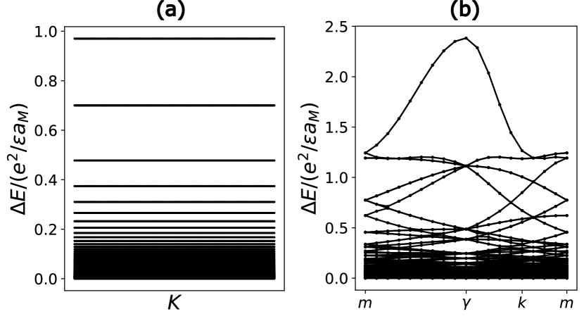
Figure 1: Two-body spectrum of the Hamiltonian (3) for $V_{n}=U_{n}$ evaluated in the $n=1$ LL when the spin of the two particles is the same (a) or opposite (b). $m-\gamma-k-m$ is a symmetry cut in the Brillouin zone. The full two-body spectrum is obtained from numerical exact diagonalization

As shown in Fig. 1, the two-particle energy spectrum in the $n=1$ LL for total spin $S_{z}=\pm 1$ and $0$ at $d=0$ (or $U_{n}=V_{n}$) are markedly different. The absence of spin $SU(2)$ symmetry results from the fact that equal-spin particles belong to the same Landau level, whereas opposite-spin particles belong to conjugate Landau levels of opposite chirality. Given the strong dependence of the energy spectrum on the total spin $S_{z}$, in order to understand our system at finite density it is essential to first determine its ground state spin polarization.

IV IV. Ferromagnetism

At the filling $\nu=1$ of the $n$-th conjugate LL pair, the fully spin polarized state with one of the two LLs completely filled is always an energy eigenstate of the band-projected Hamiltonian (3), because there is no matrix element connecting it to any other state. However, the fully polarized state may or may not be the ground state, depending on the competition between equal- and opposite-spin interactions $V_{n}$ and $U_{n}$. Obviously, the fully polarized state completely avoids the opposite-spin interaction at the expense of costing equal-spin interaction energy.

We now prove an exact result for ferromagnetism. As long as the bare interaction is spin independent and repulsive, the ground state of our system in the absence of band mixing is the fully polarized QAH state, which spontaneously breaks the $Z_{2}$ symmetry. To show this, we note that a bare interaction that is spin-independent and repulsive yields, upon projection onto the conjugate LL pair, $U_{n}=V_{n}\geq 0$ for all $\mathbf{q}$. Then, the projected Hamiltonian can be expressed in terms of the projected total density operator $\rho\equiv\rho_{+}+\rho_{-}$ as follows:

$$\tilde{H}=\frac{1}{2S_{M}}\sum_{\mathbf{q}\neq 0}V_{n}(\mathbf{q})\rho(\mathbf{q})\rho(-\mathbf{q}).$$ (14)

Here we have dropped the $\mathbf{q}=0$ term and a one-body term from normal ordering: both terms in the LL problem only depend on the total number of particles which is fixed at $\nu=1$. Importantly, Eq.(14) is manifestly semi-positive definite. Therefore, the fully polarized state with a single LL completely filled is annihilated by the projected density operator $\rho(\mathbf{q})$ for any $\mathbf{q}\neq 0$, and is necessarily a ground state of the band projected Hamiltonian.

Our exact result on full spin polarization in conjugate LL systems is consistent with a previous study of valley-degenerate LL systems with valley-dependent LL wavefunctions (which found the fully polarized ground state state within the Hartree-Fock approximation) Sodemann et al. (2017), as well as related results on ferromagnetism in certain flat band systems Bultinck et al. (2020a, b); Lian et al. (2021); Repellin et al. (2020). More importantly, our proof offers important insight into the necessary condition for the breakdown of ferromagnetism, that is, only if the repulsive interaction in the conjugate LLs is spin-dependent ($V_{n}\neq U_{n})$.

V V. Magnon Instability

To investigate the stability of ferromagnetism in our system under spin-dependent interactions, we study the energetics of the underlying single spin-flip excitation (magnon). Due to the breaking of spin $SU(2)$ symmetry by conjugate LLs, the magnon spectrum is expected to be gapped when the ground state is fully polarized. On the other hand, a negative magnon energy relative to the fully polarized state indicates that the true ground state is non-fully polarized. In this section, we analytically calculate the magnon energy in our model as a function of the spin anisotropy parameter $d$, and find it vanishes at a small $d$, which is about $15\%$ of the moire period for the $n=1$ conjugate LL (see Fig. 2). Thus, a small reduction of opposite-spin repulsion at short distance suffices to drive our system out of the fully polarized regime.

It is important to note the magnon in our system is a bound state of a particle and a hole in conjugate LLs and therefore experiences an effective magnetic field Kwan et al. (2021, 2022); Stefanidis and Sodemann (2020). As a result, the magnon energy spectrum consists of flat bands, i.e., magnon Landau levels. This should be contrasted with the magnon in quantum Hall systems which feels zero magnetic field and has a dispersive energy-momentum relation.

For the analysis below, we find it convenient to perform a particle-hole (PH) transformation of the Hamiltonian (3) on one of the spins: $c^{\dagger}_{\mathbf{k}\downarrow}\rightarrow d_{\mathbf{k}\downarrow}$. The transformed Hamiltonian then reads:

$$\tilde{H}=\frac{1}{2S_{M}}\sum_{\mathbf{q}}V_{n}(\mathbf{q})\big{[}\!:\!\rho_{\uparrow}(\mathbf{q})\rho_{\uparrow}(-\mathbf{q})\!:+:\!\overline{\rho}_{\downarrow}(\mathbf{q})\overline{\rho}_{\downarrow}(-\mathbf{q})\!:\!\big{]}\\ -\frac{1}{S_{M}}\sum_{\mathbf{q}}U_{n}(\mathbf{q}):\!\rho_{\uparrow}(\mathbf{q})\overline{\rho}_{\downarrow}(-\mathbf{q})\!:\\ +\sum_{\mathbf{k}\in{\rm BZ}}\big{[}E^{\rm HF}_{\downarrow}(\mathbf{k})\hat{N}_{\downarrow}(\mathbf{k})+E^{\rm H}_{\uparrow}(\mathbf{k})\hat{N}_{\uparrow}(\mathbf{k})\big{]}$$ (15)

where $\overline{\rho}_{\downarrow}(\mathbf{q})\sum_{\mathbf{k}}\langle\mathbf{k}+\mathbf{q}|e^{i\mathbf{q}\cdot\mathbf{R}_{\downarrow}}|\mathbf{k}\rangle d^{\dagger}_{\mathbf{k}\downarrow}d_{\mathbf{k}+\mathbf{q},\downarrow}$, $\hat{N}_{\sigma}(\mathbf{k})$ is the number operator for spin $\sigma$ and

$$E^{\rm HF}_{\downarrow}(\mathbf{k)} = \frac{1}{S_{M}}\sum_{\mathbf{k}^{\prime}\in{\rm BZ}}V_{n}(\mathbf{k}^{\prime}\mathbf{k}\mathbf{k}^{\prime}\mathbf{k}^{\prime})-V_{n}(\mathbf{k^{\prime}}\mathbf{k}\mathbf{k}\mathbf{k}^{\prime})$$

$$E^{\rm H}_{\uparrow}(\mathbf{k}) = \frac{1}{S_{M}}\sum_{\mathbf{k^{\prime}}\in{\rm BZ}}U_{n}(\mathbf{k}^{\prime}\mathbf{k}\mathbf{k}\mathbf{k}^{\prime})$$ (16)

represent the Hartree-Fock energy of a hole in a completely filled spin-$\downarrow$ LL and the Hartree energy it exerts on a spin-$\uparrow$ particle, respectively. Here $V_{n}(\mathbf{k}_{1}\mathbf{k}_{2}\mathbf{k}_{3}\mathbf{k}_{4})=\langle\mathbf{k}_{1}\sigma,\mathbf{k}_{2}\sigma|V_{n}|\mathbf{k}_{3}\sigma,\mathbf{k}_{4}\sigma\rangle$ are the matrix elements of same-spin interactions and similarly for $U_{n}(\mathbf{k}_{1}\mathbf{k}_{2}\mathbf{k}_{3}\mathbf{k}_{4})=\langle\mathbf{k}_{1}\!\!\uparrow,\mathbf{k}_{2}\!\!\downarrow\!\!|U_{n}|\mathbf{k}_{4}\!\!\uparrow,\mathbf{k}_{3}\!\!\downarrow\rangle$. Due to magnetic translation symmetry of Landau levels, both $E^{\rm HF}_{\downarrow}(\mathbf{k})$ and $E^{\rm H}_{\uparrow}(\mathbf{k})$ are independent of $\mathbf{k}$.

The above PH transformation on one of the spins maps our Hamiltonian of two time-reversal conjugate LLs to one describing two LLs in the same magnetic field as evident from the conjugated matrix elements in the the density operator $\overline{\rho}_{\downarrow}(\mathbf{q})$. However, the opposite-spin interactions become attractive as indicated from minus sign in front of $U_{n}$ in equation (15). The magnon binding energies simply become the Haldane pseudopotentials of $U_{n}(\mathbf{q})$. Relative to the fully polarized state, the magnon energy spectrum in the $n$-th LL takes the general form

$$\mathcal{E}^{m}_{n}=E^{\rm HF}_{\downarrow}+E^{\rm H}_{\uparrow}-U_{n}^{m}$$ (17)

with the Haldane pseudopotentials $U_{n}^{m}$ defined similar to equation (9) but with $U(\mathbf{q})$ instead. Consider first the case where equal spin and opposite spin interactions are the same ($V_{n}=U_{n})$. In this case, the Hartree term in $E^{\rm HF}_{\downarrow}$ and $E^{\rm H}_{\uparrow}$ cancel each other and the magnon energies simplifies to

$$\mathcal{E}^{m}_{n}=\int\frac{d^{2}\mathbf{q}}{(2\pi)^{2}}V_{n}(\mathbf{q})-U_{n}^{m}$$ (18)

The lowest spin-flip excitation energy which corresponds to the largest binding energy of the magnon ($m=0$) is

$$\mathcal{E}^{0}_{n}=\int_{0}^{\infty}\frac{qdq}{2\pi}V(q)(e^{-q^{2}l^{2}_{B}/2}-e^{-ql^{2}_{B}})[L_{n}(q^{2}l^{2}_{B}/2)]^{2}$$ (19)

When $V(\mathbf{q})>0$, it can readily seen that $\mathcal{E}^{0}_{n}>0$ in any Landau level, indicating the magnon spectrum above the fully polarized state is always gapped and hence implying robust ferromagnetism for any repulsive interaction that is spin independent.

Next, we analyze what happens when interactions are spin-dependent ($V_{n}\neq U_{n}$) and takes the form shown in equation (7). As we shall show below the lowest spin-flip excitation energy above the fully polarized state is no longer guaranteed to be positive and ferromagnetism can be destabilized.

For $d\neq 0$, the Hartree term in $E^{\rm HF}_{\downarrow}$ and $E^{\rm H}_{\uparrow}$ generally no longer cancel other and the lowest magnon energies $\mathcal{E}_{n}$ can become negative signaling an instability against ferromagnetism. For concreteness, let’s consider again Coulomb interactions $V(\mathbf{q})=\frac{2\pi e^{2}}{\epsilon|\mathbf{q}|}$, the lowest magnon energies for the $n=0$ and $n=1$ LL for generic values of $d$ are found to be

$$\mathcal{E}^{0}_{0}=\dfrac{e^{2}}{\epsilon l_{B}}\dfrac{\sqrt{\pi}}{2}(\sqrt{2}-e^{d^{2}/4l^{2}_{B}}{\rm erfc}(d/2l_{B}))+\delta E_{0}$$ (20)

$$\mathcal{E}^{0}_{1}=\dfrac{e^{2}}{\epsilon l_{B}}\frac{1}{128}\big{[}-12\frac{d}{l_{B}}+2\frac{d^{3}}{l_{B}^{3}}+48\sqrt{2\pi}-(44-4\frac{d^{2}}{l_{B}^{2}}+\frac{d^{4}}{l_{B}^{2}})e^{d^{2}/4l_{B}^{2}}\sqrt{\pi}{\rm erfc}(d/2l_{B})\big{]}+\delta E_{1}$$

$$\delta E_{n}=\frac{1}{S_{M}}\sum_{\mathbf{k}\in{\rm BZ},\mathbf{g}}[U_{n}(\mathbf{g})-V_{n}(\mathbf{g})]e^{il^{2}_{B}\mathbf{k}\wedge\mathbf{g}}$$

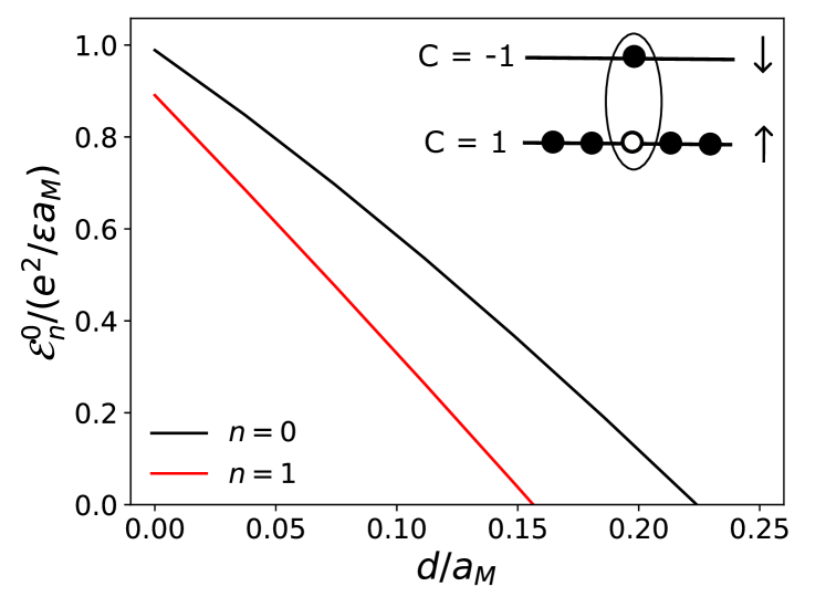
Figure 2: The lowest magnon energy $\mathcal{E}_{n}^{0}$ (equation (LABEL:eq:magnon01)) as a function of $d/aM$ calculated for the $n=0$ and $n=1$ Landau levels.

Where $\delta E_{n}$ is the difference between the Hartree energies of opposite-spin and equal spin interactions in the $n$-th Landau level and $\{\mathbf{g}\}$ denote reciprocal lattice vectors. We find the largest contribution to $\delta E_{n}$ to come from the $\mathbf{g}=0$ part such that $\delta E_{n}$ can be approximated as $\delta E_{n}\approx\frac{-e^{2}d}{\epsilon l^{2}_{B}}$. In Fig. 2, we plot $\mathcal{E}_{0}^{0}$ and $\mathcal{E}_{1}^{0}$ as a function of $d/a_{M}$. We observe the lowest magnon energy to decrease monotonically for increasing values of $d$ until it vanishes, implying that the ferromagnetic state is no longer the true ground state. A key observation is that the lowest magnon energy $\mathcal{E}_{1}^{0}$ for the $n=1$ LL vanishes faster than $\mathcal{E}_{0}^{0}$ for $n=0$ LL, meaning that ferromagnetism in the $n=1$ LL is in principle less stable against the reduction of opposite-spin interaction at short distances.

We have therefore shown that spin-dependent interactions can induce a magnon instability such that the fully polarized state is no longer the ground state. Remarkably for the $n=1$ conjugate LLs, we found that such an instability only requires a small reduction of opposite-spin interaction at very short distance ($d/a_{M}\approx 0.15$) than the moiré period, while a similar instability for the $n=0$ conjugate LLs requires a larger spin interaction anisotropy over a larger length scale.

The magnon instability indicates a transition away from the fully polarized state towards a new ground state with different spin polarization. To figure out the true ground state of the system, we analyze next the full Hamiltonian (3) across different spin sectors.

VI VI. Phase Diagram

We study the Hamiltonian (3) with exact diagonalization (ED) on finite systems. Due to $S_{z}$ spin conservation, the Hamiltonian is divided into different sectors labelled by total spin $S_{z}=(N_{\uparrow}-N_{\downarrow})/2$. We focus on two conjugate $n=1$ LLs at effective band filling factor $\nu_{\uparrow}+\nu_{\downarrow}=1$ and consider Coulomb interactions $V(\mathbf{q})=\frac{2\pi e^{2}}{\epsilon|\mathbf{q}|}$. The ED is performed on two finite momentum grids shown in Fig 3.

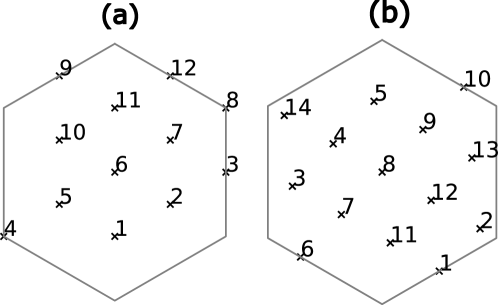
Figure 3: Finite size momentum grids used in this work. (a) 12 site cluster. (b) 14 site cluster.

To deal with the $\mathbf{q}=0$ term in both $V_{n}(\mathbf{q})$ and $U_{n}(\mathbf{q})$, we assume the existence of an identical neutralizing charge background for both spins, as physically required. However, this doesn’t fully cancel the $\mathbf{q}=0$ contribution due the anisotropy induced by finite $d$ sup and a constant term of the form $2\pi e^{2}dS_{z}^{2}/(\epsilon S_{M})$ is present and needs to be considered when comparing energies in different spin sectors MacDonald et al. (1990); Zhu et al. (2019, 2017).

We present the phase diagram in Fig. 4 showing the lowest energy state in each spin sector. For values of $d/a_{M}<0.15$, the lowest energy state across all sectors is the fully polarized state with $S_{z}=S_{\rm zmax}$, separated from other spin sectors by a finite energy gap.

When $d$ increases, we observe the magnon gap as well as the gap to other spin sectors to decrease until it vanishes. The closure of the magnon gap happens around $d/a_{M}\approx 0.15$ in agreement with our exact lowest magnon energy calculation (c.f Fig. 2). At this critical $d$ the system undergoes a direct transition to the unpolarized state with $S_{z}=0$, which remains the ground state for increasing values of $d$. It is worth noting that as the ratio of equal- to opposite-spin interactions varies, only the fully polarized and the unpolarized phases are found in our model, while partially polarized states such as considered in Refs. Stefanidis and Sodemann (2020); Kwan et al. (2021, 2022); Villadiego (2024) are not ground states of our model.

As described above, a finite $d$ parameterizes the reduction in Coulomb repulsion between opposite-spin particles at short distance up to $r\sim d$. The amount of reduction can be seen from the ratio of the largest repulsion energy $U_{1}(0)$ (equation (13) for the $n=1$ LL) at $d\neq 0$ to its Coulomb value at $d=0$ which we denote as $\eta$. As shown in the top horizontal axis of Fig. 4, the transition to the maximally unpolarized state corresponds to approximately $30\%$ reduction of $U_{1}(0)$. It is remarkable that a small modification ($30\%$) of the largest repulsive Coulomb energy corresponding to an interaction renormalization at short distance ($15\%$ of moiré period) is sufficient to drive the system from the fully polarized state into completely unpolarized one.

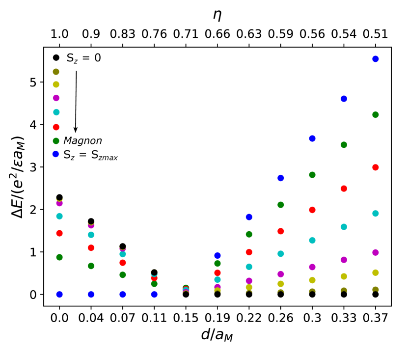
Figure 4: Phase diagram of the Hamiltonian (3) for the $n=1$ LL at effective band filling $\nu_{\uparrow}+\nu_{\downarrow}=1$ as a function of $d/a_{M}$ for spin anisotropy $d$ defined in equation (7) and $a_{M}$ is the moiré lattice constant. $S_{\rm zmax}$ is the maximum $S_{z}=(N_{\uparrow}-N_{\downarrow})/2$. $\eta$ is defined below equation (13). Calculations are done on a 14 site cluser shown in Fig. 3(b).

VII VII. non-Abelian spin Hall states

After the transition to the unpolarized phase with increasing $d$, we find a set of low-lying quasi-degenerate ground states to appear. In Fig. 5, we plot the many-body spectrum in the $S_{z}=0$ sector. We observe a low-lying ground state manifold of 36 states on a 12-unit-cell system (Fig. 5(a)) and 4 states (Fig. 5(b)) on a 14-unit-cell system. This ground state degeneracy is consistent with a product of two non-abelian Moore-Read (MR) states Moore and Read (1991) for spin-$\uparrow$ and $\downarrow$ particles in conjugate $n=1$ LLs, $|\psi\rangle=|\psi^{\uparrow}_{\text{MR}}\rangle\times|\psi^{\downarrow}_{\text{MR}}\rangle$, as a single MR state has a ground state degeneracy of 6 and 2 on even and odd site systems respectively Ardonne et al. (2008); Oshikawa et al. (2007). A state $|\psi\rangle$ of this form should exhibit ground state total momenta, $K=K_{\uparrow}+K_{\downarrow}$ where $K_{\sigma}$ is the ground state total momenta for the individual $|\psi^{\sigma}_{\text{MR}}\rangle$ which is consistent with our observation.

In addition, we present numerical evidence that the quasi-degenerante ground states are smoothly connected to the $d\rightarrow\infty$ limit, where the opposite-spin interaction vanishes. As shown in Fig. 6, the energy gap $E_{5}-E_{4}$ above the ground state manifold of 14-unit-cell system remains finite. This strongly suggests that after the spin transition, the ground state of our model stays in the same phase as two decoupled two decoupled $n=1$ Landau levels of opposite chirality, each at half filling $\nu_{\uparrow}=\nu_{\downarrow}=1/2$.

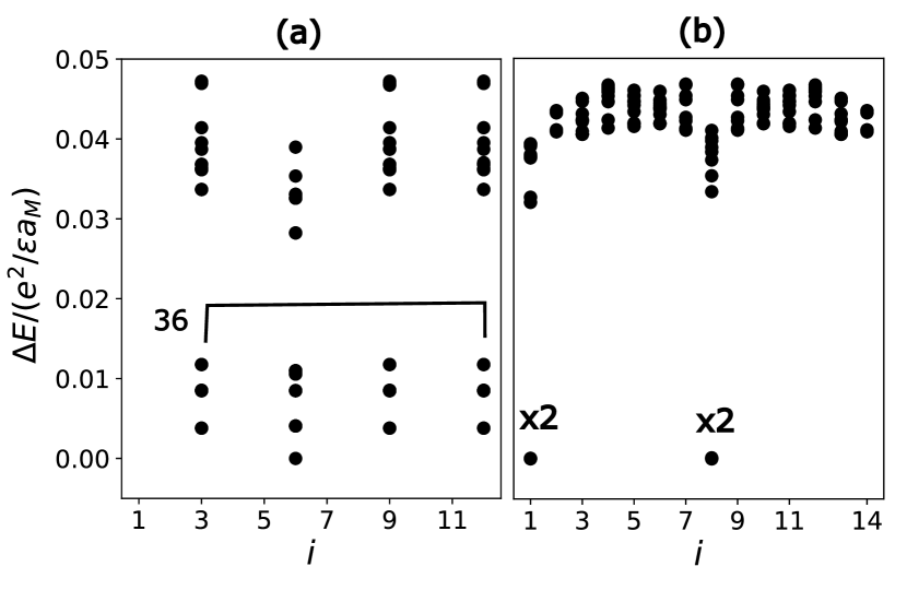
Figure 5: Many body spectrum of the Hamiltonian (3) for the $n=1$ LL at effective band filling $\nu_{\uparrow}=\nu_{\downarrow}=1/2$ or equivalently the $S_{z}=0$ sector with $d/a_{M}=0.3712$ calculated on 12-site cluster (a) shown in Fig. 3(a) and on 14 site cluster (b) shown in Fig. 3(b). The index $i$ labels the momentum points of the finite cluster.

A single $n=1$ LL with Coulomb interaction is believed to be in the non-Abelian Moore-Read phase, with the Pfaffian and anti-Pfaffian ground states being degenerate in the thermodynamic limit due to the particle-hole symmetry, which is an exact symmetry in the absence of LL mixing Lee et al. (2007); Levin et al. (2007). In our system at $d=\infty$, the state $|\psi^{\downarrow}_{\text{MR}}\rangle$ is related to $|\psi^{\uparrow}_{\text{MR}}\rangle$ by time-reversal symmetry: $|\psi^{\downarrow}_{\text{MR}}\rangle=\mathcal{T}|\psi^{\uparrow}_{\text{MR}}\rangle$. Therefore, we conclude from the mapping to $n=1$ LLs that our model in the decoupled limit $d=\infty$ exhibits $2\times 2=4$ types of ground states in the thermodynamic limit:

$$|\rm\psi_{p}\rangle = |\rm Pf\rangle_{\uparrow}\times\overline{|\rm Pf\rangle}_{\downarrow},$$

$$|\rm\psi_{a}\rangle = |\rm aPf\rangle_{\uparrow}\times\overline{|\rm aPf\rangle}_{\downarrow},$$

$$|\rm\psi_{+}\rangle = |\rm Pf\rangle_{\uparrow}\times\overline{|\rm aPf\rangle}_{\downarrow},$$

$$|\rm\psi_{-}\rangle = |\rm aPf\rangle_{\uparrow}\times\overline{|\rm Pf\rangle}_{\downarrow},$$ (21)

where the bar denotes time-reversal transformation.

The above four types of states all have non-Abelian Ising anyons with charge $e/4$ in both spin-$\uparrow$ and $\downarrow$ sectors, as well as charge $e/2$ Abelian anyons Moore and Read (1991); Read and Rezayi (1999); Greiter et al. (1991); Wen (1993). Due to the opposite chirality of conjugate LLs, they have zero electrical Hall conductivity, but exhibit quantized spin Hall effect $\sigma^{sH}=\frac{1}{2}$ and support counter-propagating charge edge modes with opposite spin. Therefore, we call these states “non-Abelian spin Hall insulators”.

Among these, $|\rm\psi_{p}\rangle$ and $|\rm\psi_{a}\rangle$ are time-reversal-invariant and map onto each other under particle-hole transformation. They represent “non-Abelian topological insulator” states at odd-integer filling, which is a non-Abelian counterpart of “fractional topological insulators” that are a product of a spin-$\uparrow$ Laughlin state and its time-reversal conjugate at fractional filling $\nu=2/(2m+1)$ Neupert et al. (2011); Repellin et al. (2014); Wu et al. (2024).

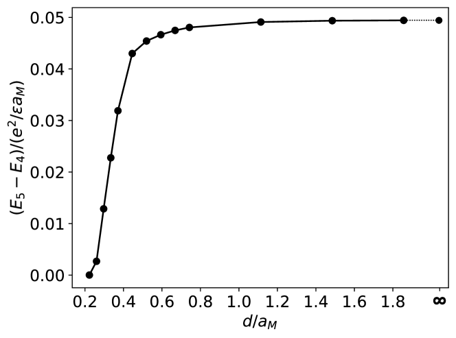
Figure 6: Energy gap $E_{5}-E_{4}$ in the $S_{z}=0$ sector of the Hamiltonian (3) on the 14 site cluster (see Fig. 3(b)) as a function of $d/a_{M}$. $d=\infty$ represents the decoupled spin $\uparrow$ and $\downarrow$ limit.

In contrast, $|\rm\psi_{\pm}\rangle$ spontaneously break time reversal symmetry and form degenerate partners. Interestingly, despite having zero electrical Hall conductivity, this time-reversal-breaking phase exhibits a quantized thermal Hall conductance and support chiral neutral edge modes. In the presence of disorder, both of these states have 4 neutral Majorana modes propagating in the same direction giving rise to a thermal Hall conductance $\kappa_{H}=\pm 2$ Kane and Fisher (1997); Read and Green (2000); Cappelli et al. (2002). Due to its time-reversal-breaking nature, this phase may also exhibit spontaneous magnetic circular dichroism.

In the decoupled limit $d=\infty$, these four states $|\rm\psi_{p,a}\rangle$ and $|\rm\psi_{\pm}\rangle$ are degenerate because each half-filled LL has its own particle-hole symmetry. At finite $d$, however, the two conjugate LLs are coupled through density-density interaction, hence our band-projected Hamiltonian only has a global particle-hole symmetry. Then, we expect the degeneracy between the time-reversal-invariant states $|\rm\psi_{p,a}\rangle$ and the time-reversal breaking states $|\rm\psi_{\pm}\rangle$ becomes lifted. Thus, the true ground state of our model at finite $d>d_{c}$ is either a non-Abelian topological insulator, or a time-reversal breaking non-Abelian state with quantized thermal Hall effect. In either case, our system is a non-Abelian helical liquid with zero electrical Hall effect and quantized spin Hall effect.

VIII VIII. Band mixing

As evident from our results, the key to overcome ferromagnetism lies in the short distance part of repulsive interaction between two particles of opposite spin. A non-zero value of $d$ effectively reduces this repulsion at short distances, while it largely doesn’t affect the long distance behavior ($\mathbf{q}\rightarrow 0$). We now show that this reduction arises naturally from the band mixing effect.

In general, band mixing is expected to renormalize the underlying interactions and therefore affect the competition between different phases as shown in the study of fractional quantum Hall systems Sodemann and MacDonald (2013); Simon and Rezayi (2013); Rezayi (2017). In our system, since spin-$\uparrow$ and $\downarrow$ particles experience opposite magnetic fields, we may expect that interactions between two particles of equal spin and of opposite spin will be renormalized by band mixing differently. Indeed, as we show explicitly below, band mixing can significantly reduce the short distance repulsion between opposite spins, which then drive the system away from ferromagnetism.

To illustrate our point, we consider a minimum model with two time-reversed pairs of flat Chern bands: (0LL, 0$\overline{\rm LL}$) and (1LL, 1$\overline{\rm LL}$). We assume that these two spinful bands are separated by an energy gap $\Delta$, while the gap to higher bands is much larger than $\Delta$. Under such condition, it is justified to neglect the contribution from higher bands and study the band mixing effect in this two-band model for interactions smaller than $\Delta$. At particle filling $\nu=3$, our two-band model can be equivalently viewed as a system of holes at filling factor $\tilde{\nu}=1$, with the vaccuum state of holes ($\tilde{\nu}=0$) corresponding to the two spinful bands completely filled with particles ($\nu=4$). This hole picture is convenient for analyzing the band mixing effect below.

When the Coulomb energy scale $E_{c}\equiv e^{2}/\epsilon a_{M}$ is small compared to the band gap $\Delta$, the holes mainly reside in 1LL and 1$\overline{\rm LL}$, with a small probability of being excited to 0LL and 0$\overline{\rm LL}$. To the leading order, the interaction between two holes in $n=1$ LL pair is simply given by the band-projected Coulomb interaction, as described earlier. The effect of band mixing appears at second order in the band mixing parameter $\kappa\equiv E_{c}/\Delta$. By second-order perturbation theory, we find that the second order correction to the equal-spin interaction psuedopotentials due to mixing with $n=0$ LL pair is given by

$$\delta V_{1}^{m}=-\kappa^{2}\frac{4\pi}{\sqrt{3}}\Bigg{[}\dfrac{\Gamma(m+1/2)\Gamma(3/2)}{2\sqrt{\pi m!(m+1)!}}\Bigg{]}^{2}$$ (22)

while the second order correction to the opposite-spin interactions reads

$$\delta U_{1}(\mathbf{R}^{\rm rel}) = -\frac{1}{\Delta^{2}}\Bigg{[}\int\frac{d^{2}\mathbf{q}}{(2\pi)^{2}}V({\mathbf{q}})[G^{\sigma}_{11}(\mathbf{q})G^{-\sigma}_{01}(-\mathbf{q})e^{i\mathbf{q}\cdot\mathbf{R}^{\rm rel}}\Bigg{]}^{2}-\frac{1}{\Delta^{2}}\Bigg{[}\int\frac{d^{2}\mathbf{q}}{(2\pi)^{2}}V({\mathbf{q}})[G^{-\sigma}_{11}(\mathbf{q})G^{\sigma}_{01}(-\mathbf{q})]e^{i\mathbf{q}\cdot\mathbf{R}^{\rm rel}}\Bigg{]}^{2}$$ (23)

$$- \frac{1}{2\Delta^{2}}\Bigg{[}\int\frac{d^{2}\mathbf{q}}{(2\pi)^{2}}V({\mathbf{q}})G^{\sigma}_{01}(\mathbf{q})G^{-\sigma}_{01}(-\mathbf{q})e^{i\mathbf{q}\cdot\mathbf{R}^{\rm rel}}\Bigg{]}^{2}$$

where $G_{nm}^{\sigma}(\mathbf{q})=\langle n|e^{i\mathbf{q}\cdot\bar{\mathbf{R}}^{\sigma}}|m\rangle$ is form factor overlap between the $n$-th LL and $m$-th LL with $\bar{\mathbf{R}}^{\sigma}$ the cyclotron orbit coordinate for spin $\sigma$ sup . The corrections to the opposite-spin interactions can be understood as consisting of three second-order processes: two which result from a hole with a certain spin scattering to the $n=0$ LL while the other hole is fixed and a third process which involve two holes both scattering to the $n=0$ LL, before scattering back to the $n=1$ LL.

To put everything together, the full Coulomb two-body energies in the $n=1$ LL to second order in $\kappa$ for equal-spin interactions are

$$\begin{gathered}\tilde{V}_{1}^{m}=\dfrac{1}{\Delta}\frac{1}{\sqrt{\sqrt{3}/4\pi}}V_{1}^{m}-\kappa^{2}\frac{4\pi}{\sqrt{3}}\Bigg{[}\dfrac{\Gamma(m+1/2)\Gamma(3/2)}{2\sqrt{\pi m!(m+1)!}}\Bigg{]}^{2}\end{gathered}$$ (24)

Where $V_{1}^{m}$ is given in equation (12). For opposite spin interactions, the expression simplifies nicely for $\mathbf{R}^{\rm rel}=0$ and we obtain

$$\begin{split}\tilde{U}_{1}(0)&=\frac{1}{\Delta}\frac{1}{\sqrt{\sqrt{3}/4\pi}}U_{1}(0)+\delta U_{1}(0)\\ &=\kappa\frac{3\pi}{4}\sqrt{\frac{1}{2\sqrt{3}}}-\kappa^{2}\frac{4\pi^{2}}{16\sqrt{3}}\end{split}$$ (25)

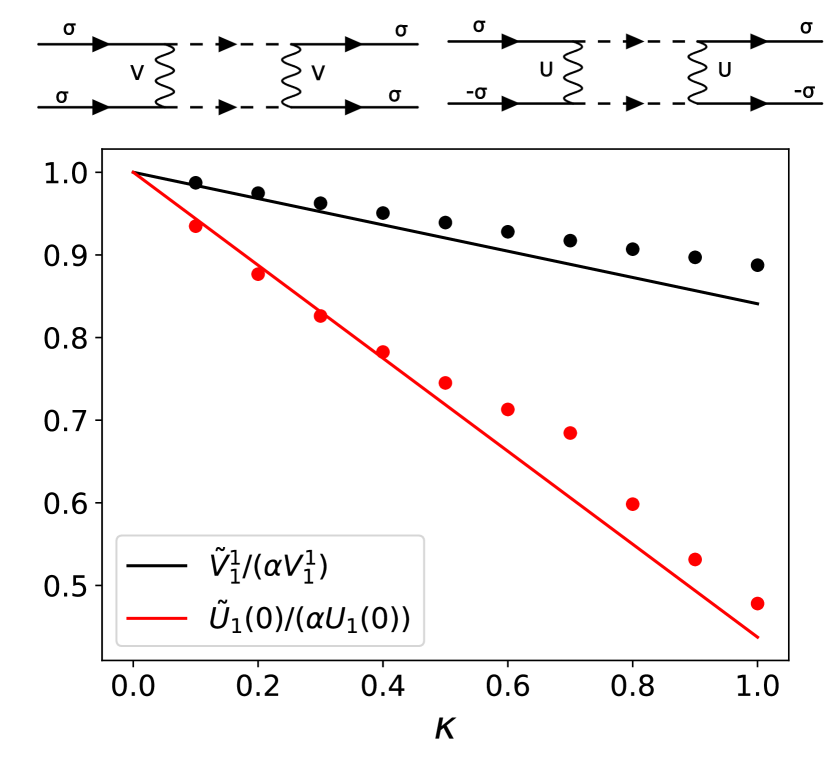
Figure 7: The largest Coulomb two body energies in the $n=1$ LL calculated to second order in $\kappa$ relative to their value at first order in $\kappa$ for equal spin and opposite spin interactions as given in equations (24) and (25). $\alpha=\frac{1}{\Delta}\frac{1}{\sqrt{\sqrt{3}/4\pi}}$. The dots are the numerically obtaiend two-body energies from exact diagonalization of the two-band model discussed. The top panel represents a schematic of a second order process that renormalizes equal-spin and opposite-spin interactions. Two holes with equal-spin (left) or opposite spin (right) scatter from the $n=1$ LL (the solid lines) to the $n=0$ LL (the dashed lines) then scatter back to the $n=1$ LL.

With $U_{1}(0)$ given in equation (13) with $d=0$. In Fig. 7., we plot the the largest repulsive components for both equal-spin ($m=1$) and opposite-spin interactions at second order in $\kappa$ relative to their values at first order in $\kappa$. We observe that opposite-spin interactions gets strongly suppressed due to band mixing. Remarkably, the reduction of opposite-spin interactions within this two-band model already reaches the needed value to drive the system out of ferromagnetism (c.f Fig. 4). While same-spin interactions gets also suppressed by band mixing, this suppression is clearly smaller than the opposite-spin case.

To confirm the validity of our perturbative calculations, we numerically diagonalize the full two-hole problem in our two-band model. As shown in Fig. 7, the numerically obtained two-body spectrum (the plotted dots) also shows strong suppression of the opposite-spin interactions due to band mixing in addition to a much weaker suppression for equal-spin interactions. For smaller values of $\kappa$, the numerical two-body energies displays excellent agreement with the values obtained perturbatively.

We have therefore established band mixing as a generic mechanism to renormalize interactions at short-distances which effectively results in a significant reduction of the opposite-spin interactions compared to equal-spin interactions even when the bare values of both are the same.

IX IX. Twisted TMD bilayers at $\nu=3$

We now discuss the relevance of our theory for twisted semiconductor bilayers. Both $t$MoTe₂ and $t$WSe₂ possess conjugate Chern bands with opposite spin Wu et al. (2019); Devakul et al. (2021). In a range of small twist angles, transport experiments have observed the quantum spin Hall effect at $\nu=2$ and the double quantum spin Hall effect at $\nu=4$ Kang et al. (2024a, b), consistent with the theoretical prediction that the lowest two moiré bands have the same spin Chern number Devakul et al. (2021); Reddy et al. (2023); Zhang et al. (2024). Moreover, near the magic angle, the approximate mapping from the first or second moiré bands to the $n=0,1$ LL has been theoretically suggested Morales-Durán et al. (2024); Reddy et al. (2024); Xu et al. (2024); Wang et al. (2024); Ahn et al. (2024); Chen et al. (2024). Therefore, despite its simplicity, our two-band model correctly captures the band topology for $t$TMD as well as the most essential feature of its moiré bands.

As evident from our magnon gap calculations (Fig. 2), ferromagnetism is more robust in the $n=0$ LL and survives larger values of spin interactions anisotropy. This can be intuitively understood due to the fact that short range repulsion, quantified by the Haldane pseudopotentials, is stronger in the $n=0$ LL than the $n=1$ LL. The absence of the quantum anomalous Hall effect at $\nu=3$ Kang et al. (2024a) in contrast to $\nu=1$ is therefore consistent with this observation. We also note that band mixing effects have been shown Abouelkomsan et al. (2024); Yu et al. (2024) to be significant in twisted TMDs. As we have shown, band mixing provides a possible mechanism for opposite-spin reduction which can drive the system away from ferromagentism.

The non-Abelian spin Hall insulators we found in our model have an insulating gap in the bulk and zero electrical Hall conductivity. Due to the doubled Moore-Read topological order, they have counter-propagating charge edge mode that are topologically protected in the presence of spin-$S_{z}$ conservation. These features are consistent with the recent transport experiment on a $t$MoTe₂ device at $\theta=2.1^{\circ}$, which found vanishing electrical Hall conductivity at $\nu=3$, accompanied with fractional edge conductance of $3e^{2}/(2h)$ over micron length scale Kang et al. (2024a).

Through a microscopic model study, we have identified two types of non-Abelian spin Hall insulators, which are time-reversal-invariant and time-reversal breaking respectively. Generally speaking, spontaneous time-reversal breaking can be detected by magnetic circular dichroism, which measures the imaginary part of Hall conductivity at optical frequency. In addition, our time-reversal-breaking non-Abelian state exhibits quantized thermal Hall conductance and supports chiral neutral edge modes.

It is worth noting that the topological order of our non-Abelian spin Hall insulators does not rely on any symmetry. Irrespective of whether time-reversal or spin-$S_{z}$ symmetry is present or not, as long as charge conservation is maintained, these non-Abelian insulators have charge $e/4$ non-Abelian anyons and, whereas recently proposed Abelian states have minimally charged anyons with charge $e/2$ Jian and Xu (2024); Zhang (2024); Villadiego (2024). Therefore, at least in principle, the presence or absence of non-Abelian fractionalization in $t$MoTe₂ can be be distinguished by measuring the fractional charge in tunneling, charge sensing and interferometer experiments.

X X. Discussion

Our model study leaves a number of important questions open for further study. The states $|\psi_{\pm}\rangle$ we identified represent a novel class of time-reversal breaking non-Abelian topological order with zero electrical Hall conductivity. Whether these states or the time-reversal-invariant ($|\psi_{p,a}\rangle$) are the true ground states can be addressed at large $d$ by treating opposite-spin interaction as a perturbation to two decoupled conjugate $n=1$ LLs. In addition, the degeneracy between time-reversal-invariant Pfaffian and anti-Pfaffian states, $|\psi_{p}\rangle$ and $|\psi_{a}\rangle$, should be lifted by band mixing, which generates three-body interactions that break particle-hole symmetry.

Regarding the time-reversal-invariant non-Abelian spin Hall insulator, an important issue is the stability of its edge state against $S_{z}$-breaking and time-reversal-invariant perturbations May-Mann et al. (2024); Cappelli and Randellini (2015) (such as Rashba spin-orbit interaction), which are expected to appear in twisted semiconductors at the edge or due to disorder. If the gapless edge states are stable in the presence of time-reversal symmetry, the non-Abelian spin Hall insulator can be regarded as a non-Abelian fractional topological insulator.

Despite its simplicity, our model is expected to host a plethora of topological phases at various fillings and under magnetic field. At high field, our model at $\nu=3$ will be a Chern insulator because spin-polarized particles completely fill the second Chern band. This is consistent with the recent transport experiment on $t$MoTe₂ at $2.6^{\circ}$ Park et al. (2024). A detailed numerical study of our model will be reported in future work.

In our analysis, we have solely considered the flat band limit. While the fully polarized state is completely insensitive to effects from non-interacting or interaction-induced dispersion, the energies of partially polarized phases can be lowered by dispersion which implies a larger window of non-ferromagnetic phases. However, dispersion can disfavor strongly interacting phases such as the non-Abelian spin Hall insulator.

Because of the underyling LL wavefunctions, our model exhibits uniform band geometry. Another important question concerns the possible effects of non-uniform band geometry which are present in twisted semiconductor bilayers. For instance, a interesting future direction is investigating the stability of ferromagnetism against band geometry fluctuations which modify the band projected interactions.

Finally, while we have focused on total filling $\nu_{\uparrow}+\nu_{\downarrow}=1$, our analysis naturally extends to other filling fractions that could support partially or completely unpolarized topologically ordered phases. In particular, we have identified band mixing as a universal microscopic mechanism for opposite-spin reduction which is a necessary ingredient for the stabilization of such phases.

XI Acknowledgements

XII Supplemental Material

XIII Landau Levels of opposite magnetic fields

Consider two dimensional electrons subject to a magnetic field, the non-interaction Hamiltonian is given by

$$H=\frac{(\mathbf{p}-e\sigma_{z}\mathbf{A})^{2}}{2m}$$ (S1)

where $\sigma_{z}=\pm 1$ denotes the two opposite magnetic fields for the two opposite spins. We work in the symmetric gauge $\mathbf{A}_{a}=-B\epsilon_{ab}\mathbf{r}_{b}/2$. The canonical momentum along with its commutation relation are are defined as

$$\begin{split}\boldsymbol{\pi}^{\sigma}=\mathbf{p}-e\sigma_{z}\mathbf{A}\\ [\boldsymbol{\pi}^{\sigma}_{a},\boldsymbol{\pi}^{\sigma}_{b}]=i\sigma_{z}\epsilon_{ab}l^{-2}_{B}\end{split}$$ (S2)

where $l_{B}=\sqrt{\hbar/eB}$ is the magnetic length. As standard in the quantum Hall problem, we define the guiding center coordinate and the cyclotron coordinate as

$$\begin{split}\mathbf{R}^{\sigma}_{a}=\mathbf{r}_{a}-l^{2}_{B}\epsilon_{ab}\boldsymbol{\pi}^{\sigma}_{b}=\mathbf{r}_{a}/2-i\sigma_{z}\epsilon_{ab}\partial_{b}\\ \bar{\mathbf{R}}^{\sigma}_{a}=l^{2}_{B}\epsilon_{ab}\boldsymbol{\pi}^{\sigma}_{b}=\mathbf{r}_{a}/2+i\sigma_{z}\epsilon_{ab}\partial_{b}\end{split}$$ (S3)

They satisfy the following algebra (for equal spin)

$$\begin{split}[\mathbf{R}^{\sigma}_{a},\mathbf{R}^{\sigma}_{b}]=-i\sigma_{z}\epsilon_{ab}l^{2}_{B}\\ [\bar{\mathbf{R}}^{\sigma}_{a},\bar{\mathbf{R}}^{\sigma}_{b}]=i\sigma_{z}\epsilon_{ab}l^{2}_{B}\\ [\mathbf{R}^{\sigma}_{a},\bar{\mathbf{R}}^{\sigma}_{b}]=0\end{split}$$ (S4)

While for opposite spins, we have the following

$$\begin{split}[\mathbf{R}^{\sigma}_{a},\mathbf{R}^{-\sigma}_{b}]=0\\ [\bar{\mathbf{R}}^{\sigma}_{a},\bar{\mathbf{R}}^{-\sigma}_{b}]=0\\ [\mathbf{R}^{\sigma}_{a},\bar{\mathbf{R}}^{-\sigma}_{b}]=-i\sigma_{z}\epsilon_{ab}l^{2}_{B}\end{split}$$ (S5)

Magnetic translations are generated by the guiding center coordinates $t^{\sigma}(\mathbf{q})=e^{i\mathbf{R}^{\sigma}\cdot\mathbf{q}}$ and they satisfy the following algebra

$$t^{\sigma}(\mathbf{q}_{1})t^{\sigma}(\mathbf{q}_{2})=e^{i\sigma_{z}l^{2}_{B}\mathbf{q}_{1}\crossproduct\mathbf{q}_{2}}t^{\sigma}(\mathbf{q}_{2})t^{\sigma}(\mathbf{q}_{1})$$ (S6)

We define a magnetic unit cell that encloses $2\pi$ flux quanta. The magnetic lattice is then spanned by $\mathbf{a}=m\mathbf{a}_{1}+n\mathbf{a}_{2}$ where $\mathbf{a}_{1}$ and $\mathbf{a}_{2}$ are two basis vectors chosen such that $|\mathbf{a}_{1}\wedge\mathbf{a}_{2}|=2\pi l^{2}_{B}$ meaning that there is one flux quanta enclosed by the unit cell. This also gives rise to magnetic reciprocal lattice basis vectors $\mathbf{g}_{1}$ and $\mathbf{g}_{2}$ such that $\mathbf{a}_{i}\cdot\mathbf{g}_{j}=2\pi\delta_{ij}$. Therefore we can apply Bloch theorem to obtain magnetic Bloch wavefunctions which we denote by $|n,\mathbf{k},\sigma\rangle$ where $n$ is a LL index and $\mathbf{k}$ is Bloch momentum. In the symmetric gauge on a torus, these are given by the modified Weierstrass sigma functions Haldane (2018). We refer the reader to the supplementary materials of Ref. Wang et al. (2021) and Ref. Reddy et al. (2024) for a detailed introduction. The Weierstrass sigma functions satisfy the boundary condition,

$$t^{\sigma}(\mathbf{g}_{i})|n,\mathbf{k},\sigma\rangle=-e^{i\sigma_{z}l^{2}_{B}\mathbf{g}_{i}\wedge\mathbf{k}}|n,\mathbf{k},\sigma\rangle$$ (S7)

The action of the magnetic translation operator for generic momentum $t^{\sigma}(\mathbf{q})$ on the magnetic Bloch state is given by

$$t^{\sigma}(\mathbf{q})|n,\mathbf{k},\sigma\rangle=e^{\frac{i}{2}l^{2}_{B}\sigma_{z}\mathbf{q}\wedge\mathbf{k}}|n,\mathbf{k}+\mathbf{q},\sigma\rangle$$ (S8)

if $\mathbf{q}$ is a reciprocal lattice basis vector then the state is transformed to itself giving rise to

$$\begin{split}t^{\sigma}(\mathbf{g}_{i})|n,\mathbf{k},\sigma\rangle=e^{\frac{i}{2}\sigma_{z}l^{2}_{B}\mathbf{g}_{i}\wedge\mathbf{k}}|n,\mathbf{k}+\mathbf{g}_{i},\sigma\rangle=-e^{i\sigma_{z}l^{2}_{B}\mathbf{g}_{i}\wedge\mathbf{k}}|n,\mathbf{k},\sigma\rangle\\ |n,\mathbf{k}+\mathbf{g}_{i},\sigma\rangle=-e^{\frac{i}{2}\sigma_{z}\mathbf{g}_{i}\wedge\mathbf{k}}|n,\mathbf{k}\sigma\rangle\end{split}$$ (S9)

Since, we are dealing with density-density interactions, we would like to evaluate the matrix elements of the density operator in the LL basis. We will utilize the transformation properties of $|n,\mathbf{k},\sigma\rangle$ under the magnetic translation operator and the fact that the relative coordinate operator can be expressed in terms of the raising and lowering operators of the LLs as follow

$$\begin{split}\bar{R}^{\uparrow}_{x}=l_{B}(\bar{a}^{\dagger}+\bar{a})/(\sqrt{2})\\ \bar{R}^{\uparrow}_{y}=l_{B}(\bar{a}^{\dagger}-\bar{a})/(\sqrt{2}i)\\ \bar{R}^{\downarrow}_{x}=l_{B}(\bar{a}^{\dagger}+\bar{a})/(\sqrt{2})\\ \bar{R}^{\downarrow}_{y}=l_{B}(\bar{a}-\bar{a}^{\dagger})/(\sqrt{2}i)\end{split}$$ (S10)

where $\bar{a}^{\dagger}|n,\mathbf{k},\sigma\rangle=\sqrt{n+1}|n+1,\mathbf{k},\sigma\rangle$. The matrix elements of the density operator can be recast as

$$\langle n_{1},\mathbf{k}_{1},\sigma|e^{i\mathbf{q}\cdot\mathbf{r}}|n_{2},\mathbf{k}_{2},\sigma\rangle=\langle n_{1},\mathbf{k}_{1},\sigma|e^{i\mathbf{q}\cdot\mathbf{\bar{R}_{\sigma}}}e^{i\mathbf{q}\cdot\mathbf{R_{\sigma}}}|n_{2},\mathbf{k}_{2},\sigma\rangle=G^{\sigma}_{n_{1}n_{2}}(\mathbf{q})F^{\sigma}({\mathbf{k}_{1},\mathbf{k}_{2}},\mathbf{q})$$ (S11)

where

$$G^{\uparrow}_{n_{1},n_{2}}(\mathbf{q})=e^{-l_{B}^{2}|\mathbf{q}|^{2}/4}\sqrt{\dfrac{n_{<}!}{n_{>}!}}L_{n_{<}}^{|n_{2}-n_{1}|}\bigg{(}\dfrac{|\mathbf{q}|^{2}l_{B}^{2}}{2}\bigg{)}\times\begin{cases}\big{(}\dfrac{-l_{B}\bar{z}}{\sqrt{2}}\big{)}^{|n_{2}-n_{1}|}&n_{2}>n_{1}\\ \big{(}\dfrac{l_{B}z}{\sqrt{2}}\big{)}^{|n_{2}-n_{1}|}&n_{1}\geq n_{2}\end{cases}$$ (S12)

$$G^{\downarrow}_{n_{1},n_{2}}(\mathbf{q})=G^{\uparrow}_{n_{2},n_{1}}(\mathbf{q})$$ (S13)

$$F^{\sigma}(\mathbf{k_{1}},\mathbf{k_{2}},\mathbf{q})=\eta_{\mathbf{g}}\delta_{\mathbf{q},\mathbf{k}_{1}-\mathbf{k}_{2}-\mathbf{g}}e^{\frac{i}{2}\sigma_{z}l_{B}^{2}((\mathbf{k}_{1}+\mathbf{k}_{2})\wedge\mathbf{g})+\mathbf{k}_{1}\wedge\mathbf{k}_{2}}$$ (S14)

where $n_{>}={\rm max}(n_{1},n_{2})$ and $n_{<}={\rm min}(n_{1},n_{2})$, $L_{a}^{b}(x)$ is the generalized Laguerre polynomial, $z=q_{x}+iq_{y}$ and $\eta_{\mathbf{g}}=1$ if $\mathbf{g}/2$ is allowed reciprocal lattice vector and $-1$ otherwise.

XIV Two body problem

In this section, we solve the two body problem for two interacting particles closely following Villadiego (2024). We consider a two body interaction $V(\mathbf{r})=V(\mathbf{r}_{1}-\mathbf{r}_{2})$ which is a function only of the relative distance. Let’s define a guiding center of mass (COM) and guiding center relative coordinate as

$$\mathbf{R}^{\rm CM}=\dfrac{\mathbf{R}^{\sigma_{1}}_{1}+\mathbf{R}^{\sigma_{2}}_{2}}{2},\>\>\mathbf{R}^{\rm rel}=\mathbf{R}^{\sigma_{1}}_{1}-\mathbf{R}^{\sigma_{2}}_{2}$$ (S15)

They satisfy the following commutation relation

$$\begin{split}[\mathbf{R}^{\rm rel}_{a},\mathbf{R}^{\rm rel}_{b}]=4[\mathbf{R}^{\rm CM}_{a},\mathbf{R}^{\rm CM}_{b}]=-il^{2}_{B}\epsilon_{ab}(\sigma_{1z}+\sigma_{2z})\\ [\mathbf{R}^{\rm CM}_{a},\mathbf{R}^{\rm rel}_{b}]=-\frac{i}{2}l^{2}_{B}\epsilon_{ab}(\sigma_{1z}-\sigma_{2z})\end{split}$$ (S16)

We see that depending on the spin of the particles either aligned or opposite, the physics of the problem can be different. We discuss the two cases below

• $\sigma_{1z}=-\sigma_{2z}$

In this case, we have $[\mathbf{R}^{\rm rel}_{a},\mathbf{R}^{\rm rel}_{b}]=[\mathbf{R}^{\rm CM}_{a},\mathbf{R}^{\rm CM}_{b}]=0$ and $[\mathbf{R}^{\rm CM}_{a},\mathbf{R}^{\rm rel}_{b}]=-il^{2}_{B}\epsilon_{ab}\sigma_{1z}$. Therefore the eigenstates can be labelled by the two coordinates $\mathbf{R}^{\rm rel}_{a}$ for $a=1,2$. Let’s denote them by $|\mathbf{R}^{\rm rel}_{a},n_{1},n_{2},\sigma_{1},\sigma_{2}\rangle$. Since, the guiding COM coordinate doesn’t commute with guiding relative coordinates, we can only label the states with one of them. We then evaluate the interaction matrix elements to get

$$\begin{split}\langle\mathbf{R}^{\rm rel}_{a},n_{1},n_{2},\sigma_{1},\sigma_{2}|\int\frac{d^{2}\mathbf{q}}{(2\pi)^{2}}U({\mathbf{q}})e^{i\mathbf{q}\cdot(\mathbf{r}^{\sigma_{1}}_{1}-\mathbf{r}^{\sigma_{2}}_{2})}|\mathbf{R}^{\rm rel}_{a},m_{1},m_{2},\sigma_{1},\sigma_{2}\rangle=\\ \langle\mathbf{R}^{\rm rel}_{a},n_{1},n_{2},\sigma_{1},\sigma_{2}|\int\frac{d^{2}\mathbf{q}}{(2\pi)^{2}}U({\mathbf{q}})e^{i\mathbf{q}\cdot(\bar{\mathbf{R}}^{\sigma_{1}}_{1}-\bar{\mathbf{R}}^{\sigma_{2}}_{2}+\mathbf{R^{\rm rel}})}|\mathbf{R}^{\rm rel}_{a},m_{1},m_{2},\sigma_{1},\sigma_{2}\rangle\\ =\int\frac{d^{2}\mathbf{q}}{(2\pi)^{2}}U({\mathbf{q}})G^{\sigma_{1}}_{n_{1}m_{1}}(\mathbf{q})G^{\sigma_{2}}_{n_{2}m_{2}}(-\mathbf{q})e^{i\mathbf{q}\cdot\mathbf{R}^{\rm rel}}\end{split}$$ (S17)

If we focus on a single Landau level denoted by $n$ and neglect mixing with the other Landau levels, then the two body energies are simply

$$U_{n}(\mathbf{R}^{\rm rel})=\int\frac{d^{2}\mathbf{q}}{(2\pi)^{2}}U({\mathbf{q}})|G^{\sigma_{1}}_{nn}(\mathbf{q})|^{2}e^{i\mathbf{q}\cdot\mathbf{R}^{\rm rel}}=\int\frac{d^{2}\mathbf{q}}{(2\pi)^{2}}U_{n}(\mathbf{q})e^{i\mathbf{q}\cdot\mathbf{R}^{\rm rel}}$$ (S18)

• $\sigma_{1z}=\sigma_{2z}$

In this case $[\mathbf{R}^{\rm CM}_{a},\mathbf{R}^{\rm rel}_{b}]=0$ and the problem reduces to the standard problem of Haldane pseudopotentials Haldane (1983). The Hamiltonian factorizes into a COM part and the relative coordinate part. The COM operators $\mathbf{R}^{\rm CM}$ describe a charged particle of $2e$ charge in magnetic field $[\mathbf{R}^{\rm CM}_{a},\mathbf{R}^{\rm CM}_{b}]=-\frac{i}{2}l^{2}_{B}\sigma_{1z}$ and $\mathbf{R}^{\rm rel}$ describe a charged particle of $e/2$ charge $[\mathbf{R}^{\rm rel}_{a},\mathbf{R}^{\rm rel}_{b}]=-2il^{2}_{B}\epsilon_{ab}\sigma_{1z}$. The two body interaction is a function only of the relative coordinates and the two-body energies (Haldane pseudopotentials) can be conveniently worked out in the symmetric gauge using the angular momemntum quantum number. For our purposes later, we will list here the Haldane psuedopotentials of the Coulomb interactions $V(\mathbf{r})=e^{2}/\epsilon\mathbf{r}$ for the $n=1$ Landau level in addition to an important matrix element Simon and Rezayi (2013)

$$V^{m}_{1}=\dfrac{e^{2}}{\epsilon l_{B}}\dfrac{\Gamma(m+1/2)}{2m!}\dfrac{(m-3/8)(m-11/8)}{(m-1/2)(m-3/2)}$$ (S19)

$$\langle n,m+n|V(\mathbf{r})|0,m\rangle=\dfrac{e^{2}}{\epsilon l_{B}}\dfrac{\Gamma(m+1/2)\Gamma(n+1/2)}{2\sqrt{\pi m!n!(n+m)!}}$$ (S20)

where $|n,m\rangle$ is a state in the $n$th Landau level with relative angular momentum $m$. Recall that the angular momentum of the $n$-th Landau level is $m-n$. So the Coulomb interaction has non-zero matrix elements only when the relative angular momentum is conserved.

XV Perturbative band mixing calculation

Here, we consider the two body problem of holes in the $n=1$ LL with mixing to the $n=0$ LL discussed in the main text. In what follows, we use Coulomb interactions $V(\mathbf{q})=\frac{2\pi e^{2}}{\epsilon|\mathbf{q}|}$ We define the Landau level mixing parameter $\kappa=E_{c}/\Delta$ where $E_{c}=e^{2}/\epsilon a_{M}$ is the Coulomb energy and $\Delta$ is the gap between the two bands. To first order in $\kappa$, the two body energies for the equal-spin interactions are simply equation (S19) while for the opposite-spin interaction interactions, they are given by equation (S18) with $n=1$.

The second order corrections to the equal-spin interactions from mixing with the $n=0$ are given by

$$\delta V_{1}^{m}=-\dfrac{|\langle 1,m+1|V(\mathbf{r})|0,m\rangle|^{2}}{\Delta^{2}}=-\kappa^{2}\frac{4\pi}{\sqrt{3}}\Bigg{[}\dfrac{\Gamma(m+1/2)\Gamma(3/2)}{2\sqrt{\pi m!(m+1)!}}\Bigg{]}^{2}$$ (S21)

where we have made use of the identity in equation (S20). In our minimal model, the second order process is simply the two holes with relative momentum $m$ in the $n=1$ LL scattering to the $n=0$ LL then scattering back to the $n=1$ LL.

To calculate the second order corrections to opposite-spin interactions, we express the opposite-spin interactions in the basis $|\mathbf{R}^{\rm rel}_{a},n_{1},n_{2},\sigma_{1},\sigma_{2}\rangle$ by defining $|n_{1},n_{2},\sigma_{1},\sigma_{2}\rangle\equiv F_{n_{1}\sigma_{1}}^{\dagger}F_{n_{2}\sigma_{2}}^{\dagger}|0\rangle$ and considering instead a modified interacting Hamiltonian $H(\mathbf{R}^{\rm rel})$. This gives to

$$H(\mathbf{R}^{\rm rel})=\frac{1}{2}\sum_{n_{1}n_{2}n_{3}n_{4},\sigma-\sigma}U^{\sigma}_{n_{1}n_{2}n_{3}n_{4}}(\mathbf{R}^{\rm rel})F^{\dagger}_{n_{1}\sigma}F^{\dagger}_{n_{2}-\sigma}F_{n_{3}-\sigma}F_{n_{4}\sigma}$$ (S22)

where $U^{\sigma}_{n_{1}n_{2}n_{3}n_{4}}(\mathbf{R}^{\rm rel})$ are the matrix elements of the opposite-spin interactions. Now consider an initial state of two holes in the $n=1$. At second order in $\kappa$, there are three types of processes. two where a hole is scattered to the $n=0$ LL with the other hole fixed and a third process where both holes scatter to the $n=1$ LL. We have then.

$$\begin{split}\delta U_{1}(\mathbf{R}^{\rm rel})=-\dfrac{|\langle 0,1,\sigma,-\sigma|H(\mathbf{R}^{\rm rel})|,1,1,\sigma,-\sigma\rangle|^{2}}{\Delta^{2}}-\dfrac{|\langle 1,0,\sigma,-\sigma|H(\mathbf{R}^{\rm rel})|1,1,\sigma,-\sigma\rangle|^{2}}{\Delta^{2}}\\ -\dfrac{|\langle 0,0,\sigma,-\sigma|H(\mathbf{R}^{\rm rel})|1,1,\sigma,-\sigma\rangle|^{2}}{\Delta^{2}}=-\frac{1}{\Delta^{2}}\Bigg{[}\int\frac{d^{2}\mathbf{q}}{(2\pi)^{2}}V({\mathbf{q}})G^{\sigma}_{01}(\mathbf{q})G^{-\sigma}_{11}(-\mathbf{q})e^{i\mathbf{q}\cdot\mathbf{R}^{\rm rel}}\Bigg{]}^{2}\\ -\frac{1}{\Delta^{2}}\Bigg{[}\int\frac{d^{2}\mathbf{q}}{(2\pi)^{2}}V({\mathbf{q}})G^{\sigma}_{11}(\mathbf{q})G^{-\sigma}_{01}(-\mathbf{q})e^{i\mathbf{q}\cdot\mathbf{R}^{\rm rel}}\Bigg{]}^{2}-\frac{1}{2\Delta^{2}}\Bigg{[}\int\frac{d^{2}\mathbf{q}}{(2\pi)^{2}}V({\mathbf{q}})G^{\uparrow}_{01}(\mathbf{q})G^{\downarrow}_{01}(-\mathbf{q})e^{i\mathbf{q}\cdot\mathbf{R}^{\rm rel}}\Bigg{]}^{2}\end{split}$$ (S23)

Putting everything together, we arrive at the expressions provided in the main text which we copy here. For equal-spin interactions, the full two body Coulomb energies are

$$\tilde{V}_{1}^{m}=\dfrac{1}{\Delta}\frac{1}{\sqrt{\sqrt{3}/4\pi}}\dfrac{\Gamma(m+1/2)}{2m!}\dfrac{(m-3/8)(m-11/8)}{(m-1/2)(m-3/2)}-\kappa^{2}\frac{4\pi}{\sqrt{3}}\Bigg{[}\dfrac{\Gamma(m+1/2)\Gamma(3/2)}{2\sqrt{\pi m!(m+1)!}}\Bigg{]}^{2}$$ (S24)

and for the opposite spin interactions interactions

$$\begin{split}\tilde{U}_{1}(\mathbf{R}^{\rm rel})=\dfrac{1}{\Delta}\int\frac{d^{2}\mathbf{q}}{(2\pi)^{2}}V({\mathbf{q}})|G^{\sigma}_{11}(\mathbf{q})|^{2}e^{i\mathbf{q}\cdot\mathbf{R}^{\rm rel}}+\delta U_{1}(\mathbf{R}^{\rm rel})\end{split}$$ (S25)

For $\mathbf{R}^{\rm Rel}=0$, the expressions simplifies to

$$\tilde{U}_{1}(0)=\kappa\frac{3\pi}{4}\sqrt{\frac{1}{2\sqrt{3}}}-\kappa^{2}\frac{4\pi^{2}}{16\sqrt{3}}$$ (S26)

XVI Interaction with neutralizing charge background

Let’s consider a generic band projected electron-electron interactions of the form

$$\begin{split}H=\frac{1}{2A}\sum_{\mathbf{k}_{1}\mathbf{k}_{2}\mathbf{q}\sigma_{1}\sigma_{2}}V_{\sigma_{1}\sigma_{2}}(\mathbf{q})F_{\sigma}(\mathbf{k}_{1},\mathbf{q})F_{\sigma}(\mathbf{k}_{2},\mathbf{q})c^{\dagger}_{\mathbf{k}_{1}+\mathbf{q}\>\sigma_{1}}c^{\dagger}_{\mathbf{k}_{2}-\mathbf{q}\>\sigma_{2}}c_{\mathbf{k}_{2}\sigma_{2}}c_{\mathbf{k}_{1}\sigma_{1}}\end{split}$$ (S27)

where $V_{\sigma_{1}\sigma_{2}}(\mathbf{q})=\frac{2\pi e^{2}}{\epsilon|\mathbf{q}|}e^{-|\mathbf{q}|d\delta_{\sigma_{1},-\sigma_{2}}}$ is the interaction. $F_{\sigma}(\mathbf{k},\mathbf{q})=\langle u_{\sigma}(\mathbf{k}+\mathbf{q})|u_{\sigma}(\mathbf{k})\rangle$ is the form factors of the band wavefunctions and $A$ is the area. We consider electrons of both spins interacting with the same uniform charge background. The Hamiltonian describing this interaction is given by

$$H_{\text{e-back}}=\frac{-e^{2}N}{A}\sum_{\sigma}\int d^{2}\mathbf{r}\int d^{2}\mathbf{R}\frac{1}{|\mathbf{r}-\mathbf{R}|}\psi_{\sigma}^{\dagger}(\mathbf{r})\psi_{\sigma}(\mathbf{r})$$ (S28)

Fourier transforming the above Hamiltonian, we have

$$\begin{split}H_{\text{e-back}}=\frac{-e^{2}N}{A}\sum_{\sigma}\sum_{\mathbf{k}}V_{\sigma\sigma}(0)\psi^{\dagger}_{\sigma}(\mathbf{k})\psi_{\sigma}(\mathbf{k})\\ =\frac{-N}{A}V(0)(N_{\uparrow}+N_{\downarrow})=\frac{-N^{2}V(0)}{A}\end{split}$$ (S29)

where $V(0)=\text{lim}_{\mathbf{q}\rightarrow 0}\frac{2\pi e^{2}}{\epsilon|\mathbf{q}|}$. In addition, the uniform background charge interacts electrostatically with itself,

$$\begin{split}H_{\text{back}}=\frac{e^{2}N^{2}}{2A^{2}}\int d^{2}\mathbf{R}\int d^{2}\mathbf{R}^{\prime}\frac{1}{|\mathbf{R}-\mathbf{R}^{\prime}|}=\frac{N^{2}V(0)}{2A}\end{split}$$ (S30)

Now, we take the limit $\mathbf{q}\rightarrow 0$ in the electron-electron Hamiltonian, we end up with two contributions, $H_{\text{lim}_{\mathbf{q}\rightarrow 0}}=H_{1}+H_{2}$

$$\begin{split}H_{1}=\frac{1}{2A}\sum_{\sigma}\text{lim}_{\mathbf{q}\rightarrow 0}V_{\sigma\sigma}(\mathbf{q})N_{\sigma}(N_{\sigma}-1)\\ H_{2}=\frac{1}{2A}\sum_{\sigma_{1}\neq\sigma_{2}}\text{lim}_{\mathbf{q}\rightarrow 0}V_{\sigma_{1}\sigma_{2}}(\mathbf{q})N_{\sigma_{1}}N_{\sigma_{2}}\end{split}$$ (S31)

Using $N_{\uparrow}N_{\downarrow}=N^{2}/4-S_{z}^{2}$ and $N_{\uparrow}^{2}+N_{\downarrow}^{2}=N^{2}/2+2S_{z}^{2}$ where $S_{z}=(N_{\uparrow}-N_{\downarrow})/2$, we end up with

$$\begin{split}H_{1}+H_{2}=\frac{1}{2A}\text{lim}_{\mathbf{q}\rightarrow 0}(V_{\uparrow\uparrow}(\mathbf{q})+V_{\uparrow\downarrow}(\mathbf{q}))\frac{N^{2}}{2}\\ +\frac{1}{A}\text{lim}_{\mathbf{q}\rightarrow 0}(V_{\uparrow\uparrow}(\mathbf{q})-V_{\uparrow\downarrow}(\mathbf{q}))S^{2}_{z}-\frac{1}{2A}V(0)N\end{split}$$ (S32)

We observe that $\text{lim}_{\mathbf{q}\rightarrow 0}(V_{\uparrow\uparrow}(\mathbf{q})-V_{\uparrow\downarrow}(\mathbf{q}))=\frac{2\pi e^{2}}{\epsilon}d$ and $\text{lim}_{\mathbf{q}\rightarrow 0}(V_{\uparrow\uparrow}(\mathbf{q})+V_{\uparrow\downarrow}(\mathbf{q}))=2V(0)$ so we get

$$H_{\text{lim}_{\mathbf{q}\rightarrow 0}}=\frac{N^{2}V(0)}{2A}-\frac{NV(0)}{2A}+\frac{2\pi e^{2}}{\epsilon}\frac{dS^{2}_{z}}{A}$$ (S33)

We see that the first term is cancelled with $H_{\text{back}}$ and $H_{\text{e-back}}$. The second term can be neglected in the thermodynamic limit Gross et al. (1991). We are therefore left with the third term which needs to be taken into account when comparing energies in different spin sectors.