Policy Gradient-Driven Noise Mask

Abstract

Deep learning classifiers face significant challenges when dealing with heterogeneous multi-modal and multi-organ biomedical datasets. The low-level feature distinguishability limited to imaging-modality hinders the classifiers’ ability to learn high-level semantic relationships, resulting in sub-optimal performance. To address this issue, image augmentation strategies are employed as regularization techniques. While additive noise input during network training is a well-established augmentation as regularization method, modern pipelines often favor more robust techniques such as dropout and weight decay. This preference stems from the observation that combining these established techniques with noise input can adversely affect model performance.

In this study, we propose a novel pretraining pipeline that learns to generate conditional noise mask specifically tailored to improve performance on multi-modal and multi-organ datasets. As a reinforcement learning algorithm, our approach employs a dual-component system comprising a very light-weight policy network that learns to sample conditional noise using a differentiable beta distribution as well as a classifier network. The policy network is trained using the reinforce algorithm to generate image-specific noise masks that regularize the classifier during pretraining. A key aspect is that the policy network’s role is limited to obtaining an intermediate (or heated) model before fine-tuning. The intermediate models might not perform well enough in direct classification task, but they are generalizable and useful in downstream tasks. During inference, the policy network is omitted and the intermediate model is fine-tuned that allows direct comparison between the baseline and noise-regularized models.

We conducted experiments and related analyses on RadImageNet datasets. Results demonstrate that fine-tuning the intermediate models consistently outperforms conventional training algorithms on both classification and generalization to unseen concept tasks. Codes, models are available at Policy-Gradient-Driven-Noise-Mask

Keywords Pretraining  $\cdot$ Medical Imaging  $\cdot$ RadImageNet  $\cdot$ Policy Gradient Method  $\cdot$ Reinforcement Learning

1 Introduction

Image classification is a fundamental task in computer vision that involves assigning labels or categories to images based on their visual content. Traditional approaches to image classification have relied on conventional supervised learning techniques, where the model is trained on a labeled dataset. However, reinforcement learning (RL) has emerged as a promising enhancement to the training process, enabling models to learn optimal classification policies through interaction with an environment[1][2]. In particular, policy gradient methods in RL offer a powerful framework for directly optimizing classification performance[3].

RL-based approaches offer a promising solution to address the challenges posed by image classification datasets[1, 4]. By learning optimal policies for feature extraction and classification through interaction with the environment, RL algorithms can adapt to the variations in low-level features and capture the relevant high-level semantic relationships [2]. This enables the development of more robust and accurate image classification models.

Medical imaging datasets, such as MRI scans, ultrasound images, and CT scans, often exhibit significant heterogeneity and variations in low-level features due to differences in acquisition protocols, imaging modalities, and anatomical regions, an example illustration is in Figure 1. These variations manifest as differences in brightness, contrast, and noise levels, which can be readily discerned even through visual inspection of image histograms. Such low-level distinguishability hinders the learning of high-level semantic relationships. The challenge is to capture and homogenize these low-level image features to improve classifier performance.

Previously, injecting random noise into the input data during training has been proposed as a regularization approach to improve generalization [5]. However, the prevalence of other powerful regularizers like weight decay and dropout raises the question of whether additional noise-based regularization is beneficial [6]. Moreover, prior work has highlighted the potential negative impact of noise-based regularization, an important consideration given that modern training pipelines typically omit additive or multiplicative noise [7].

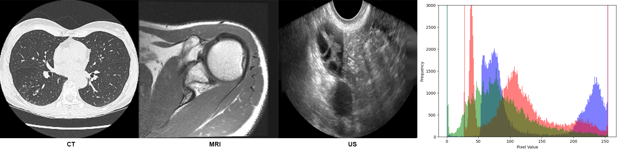
Figure 1: Heterogeneity in medical imaging datasets (RadImagenet [8]) across modalities and anatomical regions. (Left) CT scan of the lungs. (Second left) MRI scan of the shoulder. (Second Right) Ultrasound image of the ovary. (Right) Pixel intensity histograms as indicator for low-level image features of CT (blue), MRI (red), and ultrasound (green) images, illustrating variations in brightness, contrast, and noise levels.

In this paper, we present several key contributions to tackle the challenges encountered by deep learning classifiers when working with heterogeneous multi-modal and multi-organ biomedical datasets. Our primary contribution is a novel pretraining pipeline that learns to generate conditional noise masks specifically designed to enhance performance on these datasets. We propose a reinforcement learning system that consists of a lightweight policy network and a classifier network as shown in Figure 2. During pretraining, the policy network is optimized to generate image-specific noise masks that regularize the classifier, effectively improving its performance on complex biomedical datasets. This approach enables the classifier to better handle the heterogeneity and multi-modality of the data, leading to more accurate and robust predictions in various biomedical applications.

In addition to our novel pretraining pipeline, we perform comprehensive experiments and analyses on RadImageNet datasets to validate the effectiveness of our proposed approach. The results consistently show that fine-tuning the intermediate (or heated) models obtained through our pretraining pipeline outperforms conventional training algorithms on both classification tasks and generalization to unseen concepts. This superior performance underscores the potential of our reinforcement learning-based noise regularization technique in enhancing the robustness and adaptability of deep learning classifiers when faced with challenging biomedical imaging scenarios.

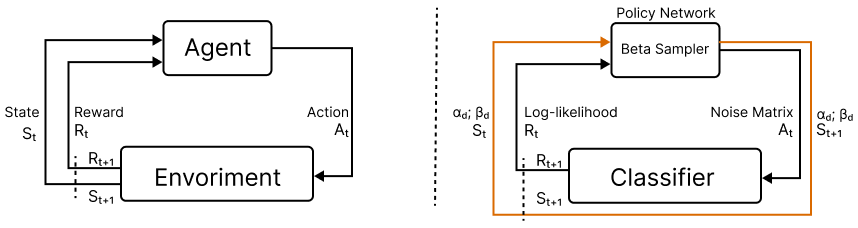
Figure 2: Schematic diagram of Reinforcement learning. At left agent takes action and change the state in environment and gain reward. At right, beta sampler (policy network) generates noise matrix and classifier as a differentiable environment computes the log-likelihood and updates the state variables $\alpha$ and $\beta$.

In summary, our contributions significantly advance the state-of-the-art in deep learning for heterogeneous multi-modal and multi-organ biomedical datasets. By introducing a novel reinforcement learning-based approach, we effectively address the limitations of existing regularization techniques and provide a powerful tool for improving the performance of deep learning classifiers in complex biomedical imaging scenarios.

The remainder of this paper is organized as follows: next sub-section provides an overview of related work in the field of medical image classification and reinforcement learning methodologies. Section 2 describes our proposed pretraining algorithm and background in detail, including training procedure. Section 3 presents the dataset, experimental setup and Section 4 includes results along with a discussion of the findings. Finally, Section 5 outlines and concludes the paper.

1.1 Literature Review

Holmstrom et al. were among the pioneers in addressing this issue by using additive noise in back-propagation training, which can be seen as an early form of regularization to prevent overfitting [9]. It is extended to the concept of the domain of speech recognition, demonstrating the effectiveness of noisy training for deep neural networks [10].

Bishop provided a theoretical foundation for training with noise, showing that it is equivalent to Tikhonov regularization, which adds a penalty term to the loss function to control the complexity of the model [5]. This concept is explored image recognition with deep neural networks in the presence of noise, demonstrating that distortions can be both a challenge and an opportunity for model training [6].

It is proposed deep neural network architectures that are robust to adversarial examples, which are inputs crafted to deceive the model into making incorrect predictions [11]. This work is part of a broader effort to develop models that maintain high performance in the presence of input perturbations.

Dropout is introduced, a simple yet effective technique to prevent neural networks from overfitting [12]. Dropout works by randomly omitting a subset of features during training, which encourages the model to learn more robust features. Further contributed to this field by introducing Cutout, a regularization method that randomly masks out sections of input images during training, forcing the network to focus on less prominent features [13].

The use of semantic segmentation for masking and cropping input images has proven to be a significant aid in medical imaging classification tasks. The proposal of a novel joint-training deep reinforcement learning framework for image augmentation called Adversarial Policy Gradient Augmentation (APGA) that shows promising results on medical imaging tasks [14].

RadImageNet, represents a significant step forward in the domain of medical imaging [8]. It is an open radiologic dataset designed to facilitate effective transfer learning in deep learning research. The MedMNIST Classification Decathlon, as presented by Yang et al., is a lightweight benchmark for medical image analysis designed to assess the capabilities of automated machine learning (AutoML) solutions [15].

2 Policy Gradient-Driven Noise Mask

We describe the mathematical formulation of the action taken by the policy network and the subsequent interaction with the environment, which leads to the computation of the loss function used for training. The order of steps follows the Figure 3 from left to right.

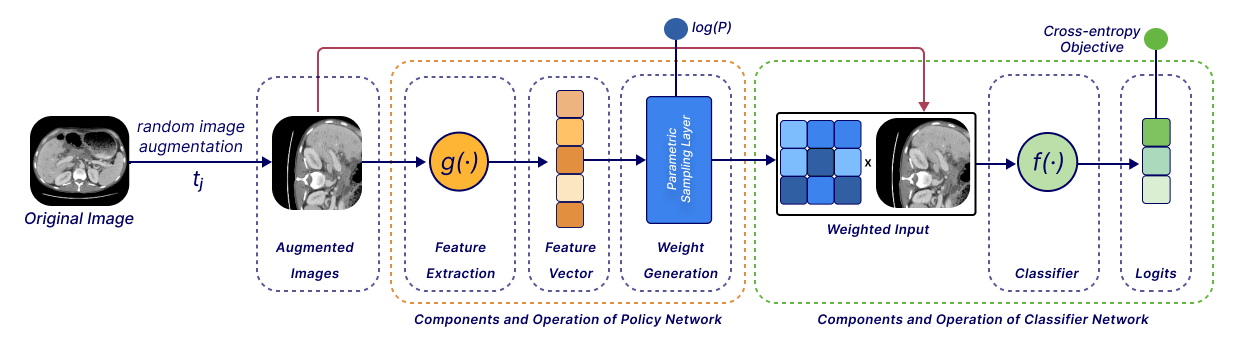
Figure 3: Diagram of our proposed pipeline using deep learning, illustrating the process from original image through stochastic masking, feature extraction, beta sampling and classification to produce a prediction with a cross-entropy objective. The blue and green color parameters to compute objective function.

Image preprocessing is the initial stage, where raw images are prepared for further processing. This step may include normalization, resizing, and other image augmentation techniques. Mathematically, if $I$ represents the raw image, the preprocessing step can be represented as:

$$I_{pre} = t_{j}(I)$$ (1)

where $I_{pre}$ is the preprocessed image and the stochastic function $t_{j}(\cdot)$ is used to obtain random augmentations of the input image j.

Action

Given an pre-processed input image $I_{pre}$, the policy network computes image specific parameters $\alpha^{\prime}$ and $\beta^{\prime}$ based on the dataset specific parameters represented by $\alpha$ and $\beta$. The updated parameters are obtained as follows:

$$\alpha^{\prime},\beta^{\prime},\alpha,\beta=\text{PolicyNet}(I,\alpha,\beta)$$ (2)

PolicyNet consists of feature extrator network $g(\cdot)$ and beta sampling operation based on features as shown in Figure 3. The extracted feature vector let the beta sampler network to generate image specific noise mask as shown in Figure 4.

These parameters are then exponentiated to ensure they are positive, as required by the Beta distribution:

$$\alpha^{\prime\prime}=e^{\alpha^{\prime}},\quad\beta^{\prime\prime}=e^{\beta^{\prime}}$$ (3)

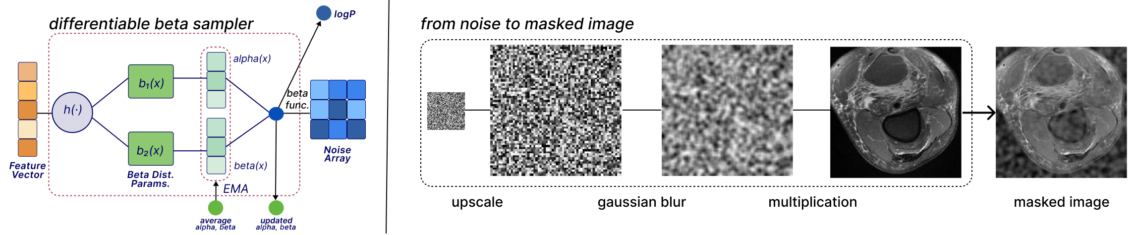
Figure 4: Diagram of a policy network architecture (at left) showing the flow from input feature tensor to weighted tensor output. The network processes the input through a function $h(\cdot)$, projects the feature vector into Beta distribution parameters $b_{1}(x)$ and $b_{2}(x)$, derives alpha and beta values for the Beta function, calculates log probability (logP). The outputs are visualized over the dashed region as colorful circles. As an example (at right), the process of applying a stochastic masking to a medical image, showcasing the transformation from a noise matrix to the final masked image, which is part of the image processing pipeline involving steps such as noise matrix acquisition, upsampling, blurring, and applying.

A Beta distribution $\mathcal{B}$ is then defined using these parameters and a mask $M$ is sampled from this distribution:

$$M\sim\mathcal{B}(\alpha^{\prime\prime},\beta^{\prime\prime})$$ (4)

The mask is reshaped to match the dimensions of the input image and then interpolated if necessary to match the image dimensions.

We also introduce post-processing steps that involve upsampling and blurring as shown in Figure 4. Firstly, we upsample the low-resolution noise matrix obtained from the policy network to obtain image regions with similar coefficient values, improving the correlation between neighboring pixels. Secondly, we apply a blurring operation to the upsampled noise matrix to avoid sharp transitions between different regions during the convolution operation, smoothing out the boundaries between areas with different noise values.

Environment The model takes the element-wise product of the input image $I$ and the mask $M_{\text{in}}$ to get the output:

$$O=\text{Model}(I_{pre}\odot M_{\text{in}})$$ (5)

Objective The log probability of the mask $M_{\text{in}}$ under the Beta distribution is computed:

$$\log(P)=\mathcal{B}.logP(M_{\text{in}})$$ (6)

The loss function is the mean of the product of the exponentiated log probabilities and the criterion applied to the output and the target:

$$\mathcal{L}=\text{mean}\left(\log\left(\sum e^{\log(P)}\right)\times\text{Criterion}(O,T)\right)$$ (7)

where $T$ represents the target labels.

Policy Gradient Method The policy gradient method aims to optimize the policy function $\pi_{\theta}(a|s)$, where $\theta$ represents the parameters of the policy, $a$ is the action taken, and $s$ is the state. The objective is to maximize the expected return $J(\theta)$, through the gradient of the objective function with respect to the policy parameters $\theta$ is given by:

$$\nabla_{\theta}J(\theta)=\mathbb{E}_{\tau\sim\pi_{\theta}}\left[\sum_{\eta=0}^{T}\nabla_{\theta}\log\pi_{\theta}(a_{\eta}|s_{\eta})R(\tau)\right]$$ (8)

where $\eta$ is the time-step. This expression allows us to update the policy parameters in the direction of increasing expected return

Image and Dataset Specific Shape Parameters The beta distribution is a continuous probability distribution defined on the interval $(0,1)$ and is parameterized by two positive shape parameters, typically denoted as $\alpha$ and $\beta$. The probability density function (PDF) of the beta distribution with parameters $\alpha$ and $\beta$ is given by:

$$f(x;\alpha,\beta)=\frac{\Gamma(\alpha+\beta)}{\Gamma(\alpha)\Gamma(\beta)}x^{\alpha-1}(1-x)^{\beta-1},\quad 0<x<1$$ (9)

where $\Gamma(\cdot)$ is the gamma function, which is a generalization of the factorial function to complex numbers.

The beta distribution is a versatile distribution that can take on various shapes depending on the values of the shape parameters $\alpha$ and $\beta$. The extracted feature vectors are transformed by a projection layer h(·) (as shown in Figure 4), which generates two separate tensors - alpha and beta - the beta distribution parameters. The beta distribution parameters - alpha and beta - are used to sample a random tensor via the beta function. This beta matrix contains values between 0 and 1. The logP output provides the log probability of this tensor under the beta distribution, which could be useful for training or interpreting the model.

The alpha and beta parameters from the last iteration step are the input for the policy network and the update function for alpha and beta are determined by recursive exponential moving averages formula:

$$\alpha_{new,image} = \tau_{i}\cdot\alpha_{dataset}+(1-\tau_{i})\cdot\alpha_{image}$$ (10)

$$\beta_{new,image} = \tau_{i}\cdot\beta_{dataset}+(1-\tau_{i})\cdot\beta_{image}$$ (11)

$$\alpha_{dataset} = \tau_{d}\cdot\alpha_{dataset}+(1-\tau_{d})\cdot\alpha_{mean,image}$$ (12)

$$\beta_{dataset} = \tau_{d}\cdot\beta_{dataset}+(1-\tau_{d})\cdot\beta_{mean,image}$$ (13)

The alpha and beta parameters in the given formulas, in a recursive manner, are used to update the Beta distribution parameters for an image-level as well as dataset-level.

The formulas use exponential moving averages to update the $\alpha$ and $\beta$ parameters for both the current image and the overall dataset:

• $\alpha_{new,image}$ and $\beta_{new,image}$ are updated by taking a weighted average of the dataset-level parameters ($\alpha_{dataset}$, $\beta_{dataset}$) and the current image-level parameters ($\alpha_{image}$, $\beta_{image}$). The weight is controlled by $\tau_{i}$, typically set to 0.9.

• $\alpha_{dataset}$ and $\beta_{dataset}$ are updated by taking a weighted average of their previous values and the mean of the image-level parameters across the dataset ($\alpha_{mean,image}$, $\beta_{mean,image}$).

Result: Optimized model parameters

Randomly initialization model parameters and dataset level $\alpha_{d}$, $\beta_{d}$;

while not converged do

       compute the $\alpha,\beta$;

       $\alpha_{i},\beta_{i},\alpha_{d},\beta_{d}\leftarrow\text{update mask params}(image,\alpha_{i},\beta_{i},\alpha_{d},\beta_{d})$;

       $\text{dist}\leftarrow\text{Beta}(\text{$\alpha_{i},\beta_{i}$})$;

       sample noise matrix;

       $\text{noise matrix}\leftarrow\text{dist.sample()}$;

       take action;

       $\text{cross entropy obj.}\leftarrow\text{classifier.step}(image,\text{noise matrix})$;

       $\text{loss}\leftarrow\text{dist.log\_prob}(\text{noise matrix})\times\text{cross entropy obj.}$;

       loss.backward();

      

end while

Algorithm 1 The policy gradient method algorithm for training policy network together with classifier mechanism.

2.1 The Algorithm

The pseudo-code for the proposed algorithm is given in Algorithm 1: Initialization The algorithm begins with the random initialization of model parameters. Additionally, dataset level parameters $\alpha_{d}$ and $\beta_{d}$ are also initialized. These parameters are crucial as they will be updated throughout the training process to optimize the regularization mechanism. Optimization The core of the algorithm is an iterative process that continues until a specified termination condition is met, which in this case is convergence. Compute Alpha and Beta At each iteration, the algorithm computes the values of $\alpha$ and $\beta$. These are the parameters of the Beta distribution, which is used to model the stochastic nature of the regularization mechanism. Update Mask Parameters The function ‘update mask params‘ is called with the current image and the alpha and beta parameters for both the individual and dataset levels. This function adjusts the parameters to better fit the data as the algorithm learns. Sample Noise Mask A noise mask is sampled from the Beta distribution parameterized by the updated $\alpha_{i}$ and $\beta_{i}$. This noise mask represents the probabilistic decisions made by the regularization mechanism at this stage of training. Take Action The classifier takes an action based on the current image and the sampled weight matrix. This step involves the classifier making a prediction which is then used to calculate the objective function, in this case, the cross-entropy loss. Calculate Loss and Backpropagate The loss is calculated by taking the log probability of the sampled weight matrix from the Beta distribution and scaling it by the cross-entropy objective. This loss is then backpropagated through the network to update the model parameters in a direction that minimizes the loss. The loop continues until convergence.

3 Experiments

Datasets For pre-training our models, we are utilizing stratified (train/val/test) split of RadImageNet [8, 16], a large-scale multi-modal and multi-organ medical imaging dataset. The split we prepare let us to justify model performance using different training techniques. This diverse dataset should help our model learn general features and representations as well as dataset specific comparison. To evaluate the performance of our pre-trained model, we are using the enhanced MedMNIST Classification Decathlon [15, 16], which includes the original 10 MedMNIST datasets, as well as 2 additional MRI datasets and 1 ultrasound (US) dataset. This comprehensive benchmark covers a wide range of medical imaging tasks, modalities (e.g., X-ray, CT, MRI, US, Microscope, OCT), and anatomical regions. By assessing our model’s performance on the enhanced MedMNIST Decathlon, we can determine how well it generalizes across various medical imaging applications.

Implementation Details The training pipeline is configured through a set of hyper-parameters. The main model to train is Resnet-50 and the policy network is always a light-weight network such as Resnet-10t. The batch size is 32 for each 8xV100 GPU with effective batch size is 256. Each training phase takes 90 epochs with SGD optimizer with learning rate 0.1, momentum 0.9 and weight decay 1e-4. The step learning rate scheduler reduce by 1/10 in 30 epochs cycle. The Resnet-10t policy network starts with 0.01 learning rate and same momentum and weight decay and using cosine annealing learning rate scheduler.

For unseen concepts, we extract the features from the freezed backbone network and using MLP for unseen concept generalization or using Logistic Regression for low-shot adaptability. Both pre-training phases use AdamW with default hyper-parameters until convergences (with no accuracy increment for 5 epochs).

3.0.1 Baselines, Ablation Study and Optimal Model

For the ablation study, we determine the optimal hyperparameters for the upscale coefficient, kernel size, and stride through a systematic search. In ablation study, we employ Resnet-10t as the backbone and the policy network due to its compact size and ease of optimization. These experiments provide a comprehensive understanding of the model’s behavior under different settings and help identify the most suitable configuration for the given task. In an evaluation task, we use Resnet50 as backbone and Resnet-10t as policy network models. Two model are compared: a baseline model and one improved training with a Gradient Policy technique. The performance (macro) metrics considered included Precision, Recall, F1 Score, AUROC, and Balanced Accuracy.

Case Analysis We investigate the scenario where no upscaling is applied, and instead, pixel-level noise is directly introduced to the input. Baseline Performance: Without any noise model applied, the performance metrics serve as a baseline. Different Noise Models: The application of Gaussian and Uniform noise models, following fine-tuning, at 32x32 and 64x64 noise matrix. Pure Noise Conditions: Under conditions simulating pure noise (noise matrix equal to image size, 224x224).

Generalization to unseen concepts We evaluate the generalization performance of our model on unseen concepts using the protocol proposed [17]. For RadImageNet, except for the modalities, the samples and classes from MedMNIST are unseen concepts. The model is pretrained on three datasets: ImageNet-1K (IN1K), RadImageNet (RadIN), and RadImageNet using Gradient Policy (Grad. P. RadIN). We then extract features for each downstream dataset and evaluate the performance using a randomly initialized multi-layer perceptron.

How fast can models adapt to unseen concepts? We evaluate the model performance for unseen concepts using low-shots proposed in [17]. We use CT, MRI, US and XR samples from MedMNIST dataset and the sample numbers are 8, 16, 32, 64, 128 and 256, respectively. The model is pretrained on three datasets: ImageNet-1K (IN1K), RadImageNet (RadIN), and RadImageNet using Gradient Policy (Grad. P. RadIN).

4 Results & Discussion

Table 1 compares the performance of lightweight Resnet-10 and baseline Resnet-50 models with and without the gradient policy technique. The intermediate models obtained by policy gradient technique is fine-tuned on RadImagenet using normal training. For both model sizes, applying the gradient policy improves all metrics, compare to normal training.

Table 1: Performance Metrics for Resnet Models with best parameter setting (Noise Matrix 64x64 and K:13 and S:6 gaussian blurring) in RadImagenet [8]

Models	Technique	Precision	Recall	F1	AUROC	Accuracy
Lightweight Model
Resnet-10t	-	0.5386	0.4262	0.4479	0.9871	0.4262
Resnet-10t	Gradient Policy	0.5659	0.4533	0.4805	0.9889	0.4533
Baseline Model
Resnet-50	-	0.5929	0.5014	0.5226	0.9884	0.5014
Resnet-50	Gradient Policy	0.6034	0.5211	0.5468	0.9900	0.5211

Table 2: The F1 scores (higher is better) indicate the generalization to unseen concepts by MedMNIST dataset [15] using Resnet-50 backbone. The results columns are for Imagenet, RadImagenet pretrained weights as well as Gradient Policy pretrained intermediate (heated) models. The t-distribution %95 confidence scores are also provided for small (7 trials) and mid-scale (3 trials) datasets.

Dataset	IN1K	RadIN	Grad. P. RadIN
Resnet-50
Small Sets (7 Trials Averaged)
Breast US	0.6662$\pm$0.0394	0.6866$\pm$0.0312	0.7649$\pm$0.0154
Breast Cancer US	0.5932$\pm$0.0137	0.5659$\pm$0.0170	0.6563$\pm$0.0111
BrainTumor MR	0.8431$\pm$0.0093	0.8275$\pm$0.0079	0.8880$\pm$0.0041
Brain MR	0.2258$\pm$0.0187	0.2257$\pm$0.0154	0.4351$\pm$0.0345
Pneumonia XR	0.8344$\pm$0.0093	0.8343$\pm$0.0085	0.8554$\pm$0.0101
Mid-scale Sets (3 Trials Averaged)
Blood Cell Mic.	0.9099$\pm$0.0024	0.8686$\pm$0.0066	0.9261$\pm$0.0024
Dermatoscope	0.4998$\pm$0.0179	0.3596$\pm$0.0602	0.4643$\pm$0.0266
OrganA CT	0.7272$\pm$0.0043	0.7339$\pm$0.0134	0.8108$\pm$0.0033
OrganC CT	0.6579$\pm$0.0119	0.6772$\pm$0.0094	0.7438$\pm$0.0037
OrganS CT	0.5622$\pm$0.0068	0.5649$\pm$0.0121	0.6170$\pm$0.0009
Large-Scale Sets (1 Trial)
Retinal OCT	0.5160	0.5220	0.5736
Colon Pathology	0.8138	0.7880	0.8042
Tissue Mic.	0.3082	0.3447	0.4033

Table 2 shows the results on enhanced medical imaging datasets. It reports the F1 scores of feature extractor Resnet-50 backbone (pretrained with ImageNet-1K, RadImageNet, and RadImageNet intermediate model with gradient policy, respectively) and evaluated using MLP over extracted feature vectors. The intermediate model with gradient policy achieves the highest F1 scores on 11 out of 13 datasets, demonstrating strong generalization to unseen medical imaging concepts. The improvements are especially significant for the small-scale datasets. It is categorized into three: the small datasets is less than 10,000 samples, mid-scale dataset range is between 10,000 and 30,000 samples, and the large-scale datasets are over 100,000 samples.

Table 3: Performance Metrics for Different Noise Models and Noise Matrix Sizes for RadImagenet [8]

Features	#Noise Matrix	Precision	Recall	F1	AUROC	Accuracy
Different Noise Models
-	-	0.5386	0.4262	0.4479	0.9871	0.4262
Gaussian + FT	32x32	0.5354	0.4273	0.4494	0.9871	0.4273
Uniform + FT	32x32	0.5206	0.4278	0.4480	0.9872	0.4278
Gaussian + FT	64x64	0.5507	0.4279	0.4497	0.9874	0.4279
Uniform + FT	64x64	0.5504	0.4299	0.4499	0.9861	0.4274
Pure Noise
-	-	0.5386	0.4262	0.4479	0.9871	0.4262
Gaussian + FT	224x224	0.5312	0.4236	0.4441	0.9864	0.4253
Gaussian + FT	224x224	0.5396	0.4312	0.4534	0.9876	0.4312
Pure Noise + FT	224x224	0.5340	0.4314	0.4555	0.9876	0.4314
Pure Noise + FT	224x224	NaN	NaN	NaN	NaN	NaN

Figures 5 reports the few-shot adaptability of each CT, MRI and US modalities in 8 different dataset and 3 pre-trained networks (ImageNet-1K, RadImageNet, and RadImageNet with gradient policy) for (8, 16, 32, 64, 128, 256 samples and 10 trials in each sample size). The orange curves are pre-trained model with gradient policy which is consistently better in few-show adaptability.

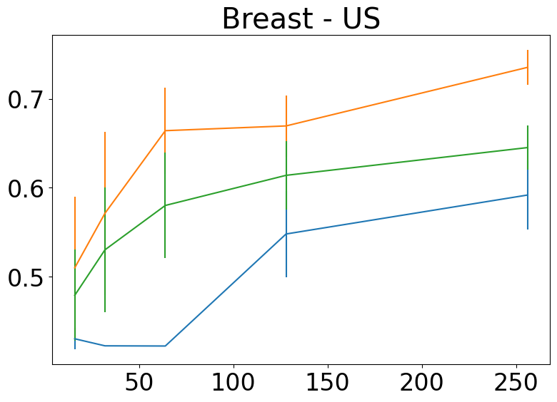
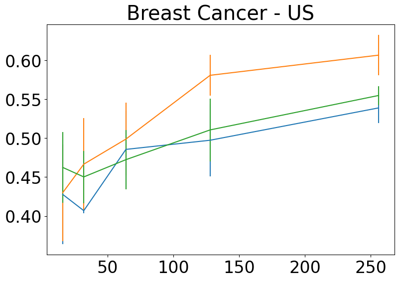
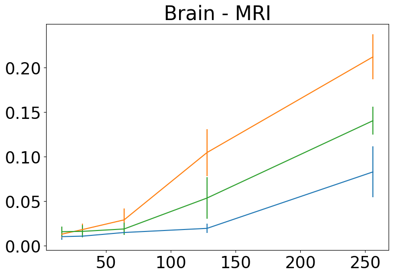
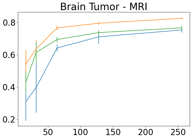
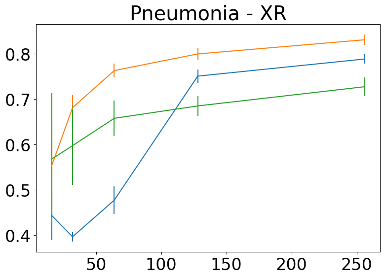
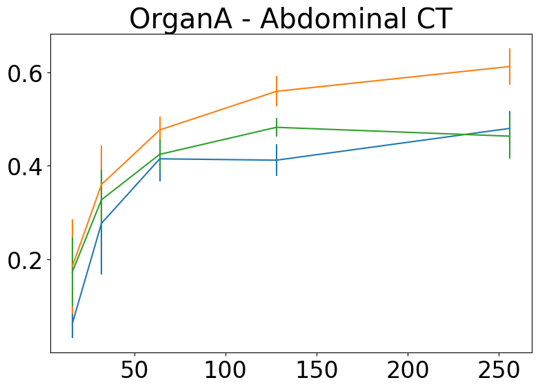
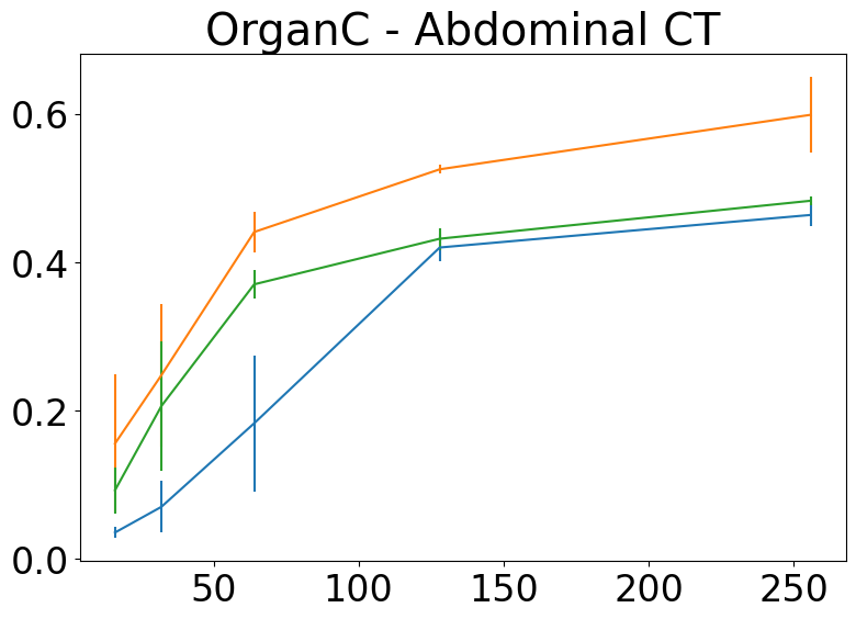
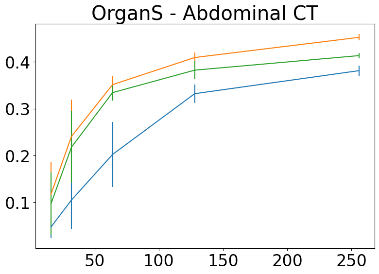
Figure 5: Each figure represents a different unseen but related dataset: Breast - US, Breast Cancer - US, Brain - MRI, Brain Tumor - MRI, Pneumonia - XR, OrganA, OrganC, OrganS - Abdominal CT. Different color curves corresponds to different pretrained model on few-shot adaptability. The orange curves represent the performance of Gradient Policy RadImagenet, the green curves show the results for ImageNet, and the blue curves indicate the performance of ImageNet pretrained models. The evaluation is carried out for 8, 16, 32, 64, 128, 256 samples and 10 trials in each sample size. The vertical lines are the t-statistics %95 confidence interval.

Table 3 shows the impact of different noise models and noise matrix sizes on the performance of the lightweight Resnet-10t model. Gaussian noise with a noise matrix of 64x64 yields the best precision, while uniform noise with a noise matrix of 64x64 gives the highest recall and accuracy. However, the differences between noise models are relatively small. Using pure noise matrix of size 224x224 leads to slightly lower but comparable performance to the baseline.

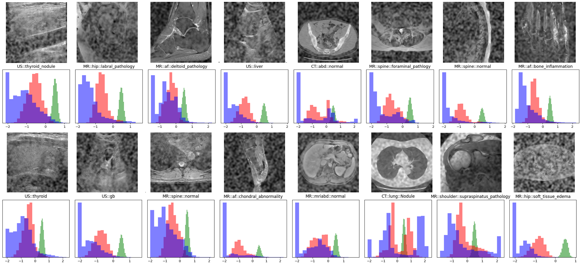
Figure 6: Composite image displaying a series of medical scans from RadImagenet [8] (1st and 3rd row) with corresponding histograms (2nd and 3rd row), where blue bars represent the original image pixel intensity distribution, red bars indicate the masked image pixel intensity distribution, and green bars show the noise pixel intensity distribution.

Figure 6 presents medical scans with their respective histograms, indicating low-level features and pixel intensity distributions. The stochastic masking operation performed by the policy network modifies the skewness and center of distribution using pixel-wise multiplication, enhancing the image representation for the classifier and achieving a form of homogenization.

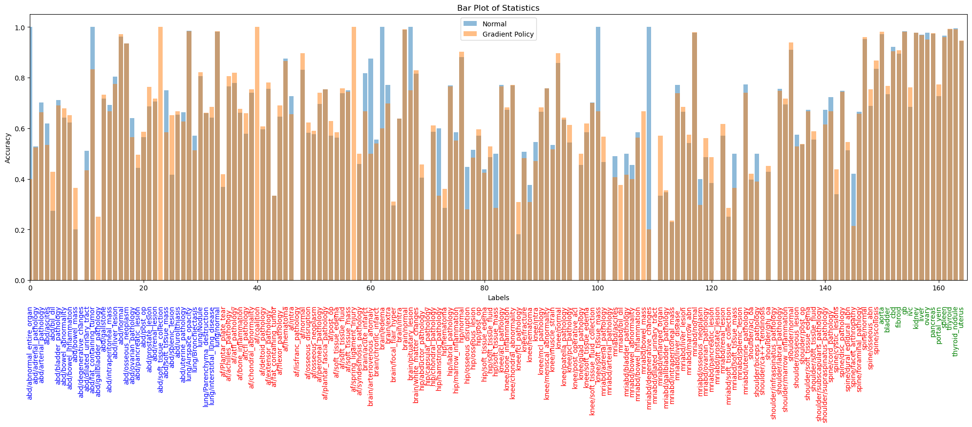
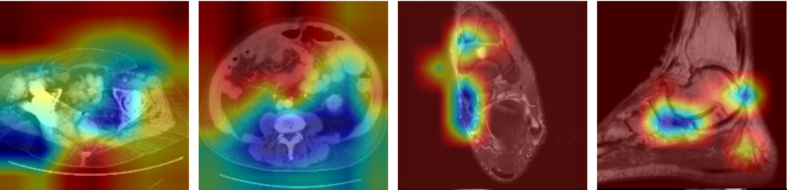
Figure 7: The top diagram shows the accuracies per label. Orange color is the model trained with gradient policy and the blue color is for conventional training. The labels are colored as well (blue is CT; red is MRI; greed is US). The bottom figures are biomedical imaging samples that are belongs to the classes that are not represented in conventional training but in Gradient Policy training. The intensity map using GradCam overlay the images (CT:abd:soft tissue collection and MR:af:coalition) and blue indicates the higher decision intensity while red is the lower decision intensity.

Figure 7 presents a comprehensive analysis comparing the gradient policy trained model to the conventional training approach. The top diagram illustrates the superior performance of the gradient policy model across various labels, while the bottom portion showcases biomedical imaging samples not represented in the conventional training dataset. Grad-CAM visualizations reveal the model’s ability to focus on relevant regions, even for unpredicted classes (CT:abd:soft tissue collection and MR:af:coalition) in the test set predictions by conventional training procedure.

The results indicate that the proposed gradient policy technique consistently improves the performance of both lightweight and larger models for medical image classification. This suggests that the gradient policy helps the models learn more robust and generalizable features. However, the performance on some unrelated datasets, such as dermatoscope images and tissue microscopy, remains relatively low. Because the low-level image features are closer to natural images by Imagenet.

Interestingly, even though the noise matrix size has an effect on our proposed model, the known distributions such as Gaussian or Uniform does not effected. The pure noise condition does not substantially impact the performance metrics either. This could imply that the model is able to effectively handle different types of noise perturbations.

An important remark on the convergence is that the dataset level $\alpha$ and $\beta$ get ‘almost‘ uniform distribution shape after beta sampling operation almost always.

It is noteworthy that our experiments conducted on natural images sourced from the Imagenet-1K dataset did not yield superior accuracy compared to existing methods, despite our best efforts and the application of novel techniques.

5 Conclusion

In summary, the Gradient Policy technique has demonstrated its effectiveness in enhancing the performance and generalization capabilities of deep learning models in biomedical image analysis. The ablation study highlights the superiority of the our proposed training schema using Gradient Policy technique over the conventional training across all performance metrics. This is achieved by fine-tuning hyper-parameters such as grid size and Gaussian blurring parameters. Moreover, the technique’s ability to improve the performance of larger models like Resnet-50 further underscores its versatility and scalability. On the other hand, the case analysis reveals that while variations in noise models such as using normal or uniform distribution or pure noise noise condition lead to minor performance differences, no statistically significant improvement is observed.

The model’s generalization performance on unseen concepts, evaluated using the protocol proposed by Sariyildiz et al., demonstrates the consistent superiority of the model pretrained on RadImageNet using Gradient Policy over models pretrained on ImageNet-1K and RadImageNet across all downstream datasets. This finding emphasizes the technique’s ability to enhance the model’s capacity to adapt to novel concepts and domains.

Furthermore, the low-shot adaptation performance on unseen concepts showcases the remarkable ability of the model pretrained on RadImageNet using Gradient Policy to quickly adapt to new concepts with limited samples, consistently outperforming models pretrained on ImageNet-1K and RadImageNet. This adaptability is crucial in the medical domain, where data scarcity and concept generalization are common challenges. The Gradient Policy technique not only improves the model’s overall accuracy but also enables it to focus on relevant features and adapt quickly to unseen concepts with limited samples.

References

- [1] Marco A Wiering, Hado Van Hasselt, Auke-Dirk Pietersma, and Lambert Schomaker. Reinforcement learning algorithms for solving classification problems. In 2011 IEEE Symposium on Adaptive Dynamic Programming and Reinforcement Learning (ADPRL), pages 91–96. IEEE, 2011.
- [2] Soumyendu Sarkar, Ashwin Ramesh Babu, Vineet Gundecha, Antonio Guillen, Sajad Mousavi, Ricardo Luna, Sahand Ghorbanpour, and Avisek Naug. Rl-cam: Visual explanations for convolutional networks using reinforcement learning. In Proceedings of the IEEE/CVF Conference on Computer Vision and Pattern Recognition, pages 3860–3868, 2023.
- [3] Fadi AlMahamid and Katarina Grolinger. Reinforcement learning algorithms: An overview and classification. In 2021 IEEE Canadian Conference on Electrical and Computer Engineering (CCECE), pages 1–7. IEEE, 2021.
- [4] Masato Fujitake. Rl-logo: Deep reinforcement learning localization for logo recognition. In ICASSP 2024-2024 IEEE International Conference on Acoustics, Speech and Signal Processing (ICASSP), pages 2830–2834. IEEE, 2024.
- [5] CM Bishop. Training with noise is equivalent to tikhonov regularization. Neural computation, 7(1):108–116, 1995.
- [6] Michał Koziarski and Bogusław Cyganek. Image recognition with deep neural networks in presence of noise–dealing with and taking advantage of distortions. Integrated Computer-Aided Engineering, 24(4):337–349, 2017.
- [7] M Eren Akbiyik. Data augmentation in training cnns: injecting noise to images. arXiv preprint arXiv:2307.06855, 2023.
- [8] Xueyan Mei, Zelong Liu, Philip M Robson, Brett Marinelli, Mingqian Huang, Amish Doshi, Adam Jacobi, Chendi Cao, Katherine E Link, Thomas Yang, et al. Radimagenet: an open radiologic deep learning research dataset for effective transfer learning. Radiology: Artificial Intelligence, 4(5):e210315, 2022.
- [9] L Holmstrom and P Koistinen. Using additive noise in back-propagation training. IEEE Trans Neural Netw, 3(1):24–38, 1992.
- [10] S Yin, C Liu, Z Zhang, Y Lin, D Wang, J Tejedor, et al. Noisy training for deep neural networks in speech recognition. EURASIP Journal on Audio, Speech, and Music Processing, 2015:1–14, 2015.
- [11] S Gu and L Rigazio. Towards deep neural network architectures robust to adversarial examples. arXiv preprint arXiv:1412.5068, 2014.
- [12] N Srivastava, G Hinton, A Krizhevsky, I Sutskever, and R Salakhutdinov. Dropout: a simple way to prevent neural networks from overfitting. The journal of machine learning research, 15(1):1929–1958, 2014.
- [13] T DeVries and GW Taylor. Improved regularization of convolutional neural networks with cutout. arXiv preprint arXiv:1708.04552, 2017.
- [14] Kaiyang Cheng, Claudia Iriondo, Francesco Calivá, Justin Krogue, Sharmila Majumdar, and Valentina Pedoia. Adversarial policy gradient for deep learning image augmentation. In Medical Image Computing and Computer Assisted Intervention–MICCAI 2019: 22nd International Conference, Shenzhen, China, October 13–17, 2019, Proceedings, Part VI 22, pages 450–458. Springer, 2019.
- [15] J Yang, R Shi, and B Ni. Medmnist classification decathlon: A lightweight automl benchmark for medical image analysis. In 2021 IEEE 18th International Symposium on Biomedical Imaging (ISBI), pages 191–195. IEEE, 2021.
- [16] Mehmet Can Yavuz and Yang Yang. Refined radimagenet: Artifacts and analyses. arXiv preprint arXiv, 2024.
- [17] Mert Bulent Sariyildiz, Yannis Kalantidis, Diane Larlus, and Karteek Alahari. Concept generalization in visual representation learning. In International Conference on Computer Vision, 2021.