Phase distribution in 1D localization
and phase transitions in single-mode waveguides

1. Introduction

Localization of electrons in 1D disordered systems can be conveniently described using the transfer matrix $T$, relating the amplitudes of plane waves on the left ($Ae^{ikx}+Be^{-ikx}$) and on the right ($Ce^{ikx}+De^{-ikx}$) of a scatterer,

$$\left(\begin{array}[]{cc}A\\ B\end{array}\right)\,=T\left(\begin{array}[]{cc}C\\ D\end{array}\right)\,.$$

In the presence of the time-reversal invariance, the matrix $T$ can be parametrized in the form [1]

$$T=\left(\begin{array}[]{cc}\!\!\!1/t\!&\!-r/t\!\!\\ \!\!-r^{*}/t^{*}\!&\!1/t^{*}\!\!\!\end{array}\right)\,=\left(\begin{array}[]{cc}\!\!\sqrt{\rho\!+\!1}\,e^{i\varphi}\!\!&\!\!\sqrt{\rho}\,e^{i\theta}\!\!\\ \!\!\sqrt{\rho}\,e^{-i\theta}\!\!&\!\!\sqrt{\rho\!+\!1}\,e^{-i\varphi}\!\!\end{array}\right)\,,$$

where $t$ and $r$ are the amplitudes of transmission and reflection, while $\rho=|r/t|^{2}$ is the dimensionless Landauer resistance [2]. For the successive arrangement of scatterers their transfer matrices are multiplied. For a weak scatterer its transfer matrix $T$ is close to the unit one, allowing one to derive the differential evolution equations for its parameters.

Usually, such equations are derived in the random phase approximation, when distributions of $\varphi$ and $\theta$ are considered as uniform [3]–[8]. Such approximation is working sufficiently good for weak disorder in the deep of the allowed band, as it is usually accepted in theoretical papers (see references in [9, 10, 11]). The fluctuation states in the forbidden band are considered infrequently [12, 13, 14] and only on the level of wave functions. A systematic analysis shows that the random phase approximation is strongly violated near the initial band edge and in the forbidden band of an ideal crystal [15]. In the general case, the evolution equations are written in terms of the Landauer resistance $\rho$ and the combined phases (Sec.2)

$$\psi=\theta-\varphi\,,\qquad\chi=\theta+\varphi\,.$$

The phase $\chi$ does not affect the evolution of $\rho$ and is not interesting for the condensed matter physics; so it was not discussed in the previous papers [15, 16, 17]. Optical measurements (see below) allow to study the distribution of the phase $\chi$, and its theoretical investigation becomes actual.

The complete evolution equation for the distribution $P(\rho,\psi,\chi)$ is derived in Appendix. In fact, it has no practical value, and only its general structure is essential, which allows separation of variables (Sec.2). Factorization $P(\rho,\psi,\chi)=P(\rho,\psi)P(\chi)$ is valid for an arbitrary system length $L$, and allows to confine oneself to equations for $P(\rho,\psi)$ and $P(\chi)$. Additional factorization $P(\rho,\psi)=P(\rho)P(\psi)$ arises for large $L$ and leads to the closed equation for $P(\rho)$ and the equation for the stationary distribution $P(\psi)$.

The stationary distribution of the phase $\psi$ was studied in the papers [16, 17]; in the deep of the disordered system it undergoes the peculiar phase transition in the point ${\cal E}_{0}$, when the electron energy ${\cal E}$ is changed [17], consisting in appearance of the imaginary part of $\psi$ (Sec.3). Meanwhile, the distribution of resistance $P(\rho)$ has no singularity at the point ${\cal E}_{0}$, and the transition looks unobservable in the framework of condensed matter physics.

The evolution equation for $P(\chi)$ is derived in Sec.4: it has a form of the usual diffusion equation, where the diffusion constant and drift velocity are exponential functions of $L$. The corresponded exponentials have singularities as functions of ${\cal E}$, consisting in jumps of the second derivative (Sec.5). Such phase transitions are also unobservable for the electron disordered systems.

However, the approach developed previously [15, 16, 17] is immediately applicable to the scattering of waves propagating in single-mode optical waveguides (Sec.6.1). Existent optical methods (heterodyne approach, near-field microscopy, etc.) are rather efficient, and allow to measure distributions of all parameters $\rho$, $\psi$, $\chi$ inside the waveguide  (Sec.6.3). It extends the observable aspects of the 1D localization theory, and provides possibilities for its deep experimental verification. In particular, the phase transitions in distributions $P(\psi)$ and $P(\chi)$ become observable (Secs.6.2, 6.3). The possible schemes of measurement are described in Sec.6.4.

The brief communication on the obtained results was made previously by the author and S. I. Bozhevolnyi [18].

2. General structure of evolution equations

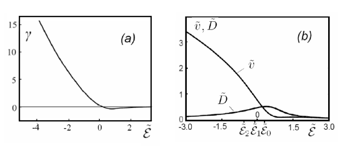
Figure 1: Dependence of parameters $\gamma$, $\tilde{v}=v/W^{2/3}$ and $\tilde{D}=D/W^{2/3}$ on the reduced energy $\tilde{\cal E}={\cal E}/W^{4/3}$, obtained from the analysis of moments for the transfer matrix elements [15]. These moments are regular functions of energy, which leads to regularity of the presented dependencies. Smallness of $\gamma$ and the equality $v=D$, valid in the random phase approximation, are realized only in the deep of the allowed band. The points $\tilde{\cal E}_{0}$, $\tilde{\cal E}_{1}$, $\tilde{\cal E}_{2}$ correspond to phase transitions, discussed in Secs.3, 5.

The most general evolution equation describes the change of the mutual distribution $P(\rho,\psi,\chi)$ under increasing of the system length $L$ and has the following structure (see Appendix)

$$\frac{\partial P}{\partial L}=\left\{\vphantom{L^{2}}\hat{L}_{\rho,\psi}P\right\}^{\prime}_{\rho}+\left\{\vphantom{L^{2}}\hat{M}_{\rho,\psi}P\right\}^{\prime}_{\psi}\,+\left\{\vphantom{L^{2}}\hat{K}_{\rho,\psi,\chi}P\right\}^{\prime}_{\chi}\,,$$

where $\hat{K}$, $\hat{L}$, $\hat{M}$ are operators, depending on indicated variables. The right-hand side is the sum of full derivatives, which ensures the conservation of probability. As was discussed in [17, 19], conditions for separation of variables in the diffusion-type equations are essentially weaker, than for an eigenvalue problem. Independence of $\chi$ for operators $\hat{L}$ and $\hat{M}$ provides factorization $P(\rho,\psi,\chi)=P(\rho,\psi)P(\chi)$, where $P(\rho,\psi)$ and $P(\chi)$ are determined by equations

$$\frac{\partial P(\rho,\psi)}{\partial L}=\left\{\vphantom{L^{2}}\hat{L}_{\rho,\psi}P(\rho,\psi)\right\}^{\prime}_{\rho}+\left\{\vphantom{L^{2}}\hat{M}_{\rho,\psi}P(\rho,\psi)\right\}^{\prime}_{\psi}$$

and

$$\frac{\partial P(\chi)}{\partial L}=\left\{\vphantom{L^{2}}\hat{\cal K}_{\chi}P(\chi)\right\}^{\prime}_{\chi}\,,\quad\hat{\cal K}_{\chi}=\int\hat{K}_{\rho,\psi,\chi}P(\rho,\psi)\,d\rho\,d\psi\,.$$

The specific form of Eq.5 is given in [16, 17], while Eq.6 is derived in Sec.4. In the large $L$ limit, when the typical values of $\rho$ are large, the operator $\hat{M}_{\rho,\psi}$ becomes independent of $\rho$; then the solution of Eq.5 is factorized, $P(\rho,\psi)=P(\rho)P(\psi)$, where $P(\rho)$ and $P(\psi)$ are determined by equations

$$\frac{\partial P(\psi)}{\partial L}=\left\{\vphantom{L^{2}}\hat{M}_{\psi}P(\psi)\right\}^{\prime}_{\psi}\,,$$

$$\frac{\partial P(\rho)}{\partial L}=\left\{\vphantom{L^{2}}\hat{\cal L}_{\rho}P(\rho)\right\}^{\prime}_{\rho}\,,\quad\hat{\cal L}_{\rho}=\int\hat{L}_{\rho,\psi}P(\psi)\,d\psi\,.$$

Equation (7) provides the existence of the stationary distribution of the phase $\psi$. The equation (8) for $P(\rho)$ has a form [15]

$$\frac{\partial P(\rho)}{\partial L}=D\,\frac{\partial}{\partial\rho}\left[\,-\gamma(1\!+\!2\rho)P(\rho)+\rho(1\!+\!\rho)\,\frac{\partial P(\rho)}{\partial\rho}\,\right]\,,$$

and gives at large $L$ the limiting log-normal distribution

$$P(\rho)=\frac{1}{\rho\sqrt{4\pi DL}}\exp\left\{-\frac{[\ln\rho-vL]^{2}}{4DL}\right\}\,$$

with $v=(2\gamma\!+\!1)D$. The typical value of $\rho$ increases exponentially with $L$, which is an observable manifestation of 1D localization. In the random phase approximation, the parameter $\gamma$ turns to zero, and equations (9), (10) coincide with the previously obtained results [3]–[8]. Dependencies of $\gamma$, $D$, $v$ on the reduced energy $\tilde{\cal E}={\cal E}/W^{4/3}$, obtained from the analysis of moments for distribution of the transfer matrix elements [15], are shown in Fig.1, where ${\cal E}$ is the energy counted from the initial band edge, and $W$ is an amplitude of the random potential; all energies are measured in units of the hopping integral of the 1D Anderson model, which is of the order of the initial band width. Strong violation of the random phase approximation is thereby evident (Fig.1).

It should be clear that the specific form of Eq.4 is of no importance, and only its general structure is essential. For arbitrary $L$, Eq.4 is split to two equations (5) and (6), while for large $L$ it reduces to three equations (6), (7), (8). It is also clear, that the choice of independent variables $\rho$, $\psi$, $\chi$ has the objective character.

3. Phase transition in the distribution $P(\psi)$

The meaning of the phase transition in the $\psi$ distribution consists in the fact that difference between the allowed and forbidden bands survives (in a certain sense) in the presence of the random potential, though a singularity in the density of states is smoothed out. It resembles the famous argumentation by Mott [20], that the role of the allowed band edge comes to the mobility edge. Although the mobility edge is absent in the 1D case, a ’trace’ of it still remains. The point is that the probe scatterer in the allowed band (${\cal E}>0$) is described by the transfer matrix (2), while in the forbidden band (${\cal E}<0$) it is described by the pseudo-transfer matrix ${\cal T}$ [15], relating coefficients of the increasing and decreasing exponents on the left ($Ae^{\kappa x}+Be^{-\kappa x}$) and on the right ($Ce^{\kappa x}+De^{-\kappa x}$) of the scatterer. In the simplest case, the matrix ${\cal T}$ is real and corresponds to pure imaginary values of phases $\theta$ and $\varphi$. Let us compare situations for ${\cal E}>0$ and ${\cal E}<0$: for a sufficient separation in energy, the difference between two types of matrices can be made arbitrary large, and it cannot be overcome by addition of weak disorder. As a result, the border-line between the true and pseudo transfer matrices can only be shifted, but not eliminated. In practice, it is manifested via the appearance of the imaginary part of the phase $\psi$ for energies ${\cal E}<{\cal E}_{0}$ [17].

The formal statements of the paper [17] reduce to the following. First of all, one should differ the ’external’ and ’internal’ phase distributions (Fig.2). The internal phase distribution is realized in the deep of a sufficiently long disordered system, and is independent of boundary conditions. Considering the system from the side of ideal leads, one observes the ’external’ phase distribution, which is determined by the boundary conditions; namely these phases appear in the transfer matrix. Influence of interfaces extends till the length scale of the order of the localization length $\xi$: it determines the transient region, where the internal phase distribution continually transforms to the external one. In the large $L$ limit, the distribution $P(\rho)$ is determined by the internal phase distribution, which provides its independence from the boundary conditions. However, the evolution equations contain namely the external phase distribution, and one wonders why it does not affect the limiting distribution $P(\rho)$. The second question, related with the first one, is as follows: how can we find the internal phase distribution, if it does not appear in the evolution equations?

The above questions are resolved in the following manner. The phase $\psi$ appears to be a ’bad’ variable, while the ’correct’ variable is

$$w=-{\rm cot}\,\psi/2\,.$$

The form of the stationary distribution $P(w)$ is determined by the internal properties of the system and does not depend on the boundary conditions. If the boundary conditions are changed, it leads to three effects: the scale transformation $w\to sw$ and two translations $w\to w+w_{0}$ and $\psi\to\psi+\psi_{0}$. The corresponding changes of the distribution $P(\psi)$ are easily predictable [17] and can be observed in the external phase distribution. The evolution equations are invariant in respect to translation $\psi\to\psi+\psi_{0}$, and the internal phase distribution can be discussed at some fixed choice of the origin. Invariance of the limiting distribution $P(\rho)$ under transformations $w\to sw$ and $w\to w+w_{0}$ is realized in the dynamical manner. Analogously to aperiodic oscillations of $P(\rho)$ [21, 22], in the region $L\mathbin{\lower 3.0pt\hbox{$\hbox to0.0pt{\raise 5.0pt\hbox{$\char 60\relax$}\hss}\mathchar 29208\relax$}}\xi$ the scale factor $s$ and the translational shift $w_{0}$ undergo aperiodic oscillations as functions of $L$, attenuating at large $L$. As a result, $s$ and $w_{0}$ tend to the certain ’correct’ values, which provide the correct values of $D$ and $v$ in the limiting distribution (10). The indicated ’correct’ values  correspond to the internal phase distribution, and the latter can be found after return to the variable $\psi$. Meanwhile, it appears that the translational shift $w_{0}$ becomes complex-valued for ${\cal E}<{\cal E}_{0}$, indicating the appearance of the imaginary part of $\psi$. This qualitative change indicates the existence of the unusual phase transition.

The point ${\cal E}_{0}$ is not singular for the Landauer resistance $\rho$, and the whole distribution $P(\rho)$ varies in its vicinity in a smooth manner (Fig.1,b). As a result, the described phase transition looks unobservable in the framework of the condensed matter physics. Fortunately, it has the observable manifestations in optics in the form of the square root singularities in the frequency dependencies (Secs.6.2,6.3).

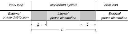
Figure 2: External and internal phase distributions.

4. Evolution equation for $P(\chi)$

According to [17], the change of the transfer matrix $T^{(n)}$ under increasing the number of scatterers $n$ is determined by the recurrence relation

$$T^{(n+1)}=T^{(n)}T_{\delta}T_{\epsilon_{n}}\,,$$

where matrices $T^{(n)}$ and $T_{\epsilon_{n}}$ are statistically independent, and $T_{\delta}$ is constant. These matrices can be accepted in the form

$$T_{\epsilon_{n}}=\left(\begin{array}[]{cc}1\!-\!i\epsilon_{n}&\epsilon_{n}{\rm e}^{i\gamma}\\ \epsilon_{n}{\rm e}^{-i\gamma}&1\!+\!i\epsilon_{n}\end{array}\right)\,,\qquad$$

$$T_{\delta}=\left(\begin{array}[]{cc}{\cal A}&{\cal B}\\ {\cal B}^{*}&{\cal A}^{*}\end{array}\right)\,=\left(\begin{array}[]{cc}\sqrt{1\!+\!\Delta^{2}}\,{\rm e}^{i\alpha}\!\!&\Delta{\rm e}^{i\beta}\!\!\!\\ \Delta{\rm e}^{-i\beta}\!&\sqrt{1\!+\!\Delta^{2}}\,{\rm e}^{-i\alpha}\!\!\end{array}\right).$$

where $\epsilon_{n}$ is proportional to the amplitude of the $n$th scatterers, and $\langle\epsilon_{n}\rangle=0$, $\left\langle\epsilon^{2}_{n}\right\rangle\equiv\epsilon^{2}$, while $T_{\delta}$ is determined by the parameter $\delta$, proportional to the distance between scatterers , so that $\Delta\sim\alpha\sim\delta$ [17]. Below we consider the limit

$$\delta\to 0\,,\quad\epsilon\to 0\,,\quad\delta/\epsilon^{2}=const$$

and retain the terms of the first order in $\delta$ and the second order in $\epsilon$.

Accepting parametrization (2) for $T^{(n)}$ and denoting parameters of $T^{(n+1)}$ as $\tilde{\rho}$, $\tilde{\varphi}$, $\tilde{\theta}$, we have

$$\sqrt{1\!+\!\tilde{\rho}}\,{\rm e}^{i\tilde{\varphi}}=\sqrt{1\!+\!\rho}\,{\rm e}^{i\varphi}({\cal A}+\epsilon{\cal C})+\sqrt{\rho}\,{\rm e}^{i\theta}({\cal B}^{*}\!+\epsilon{\cal D}^{*})\,,$$

$$\sqrt{\tilde{\rho}}\,{\rm e}^{i\tilde{\theta}}=\sqrt{1\!+\!\rho}\,{\rm e}^{i\varphi}({\cal B}\!+\!\epsilon{\cal D})+\sqrt{\rho}\,{\rm e}^{i\theta}({\cal A}^{*}\!+\epsilon{\cal C}^{*})\,,$$

where the following notations are accepted

$${\cal C}=\!{\cal B}\,{\rm e}^{-i\gamma}\!-\!i{\cal A}\,\qquad{\cal D}=\!{\cal A}\,{\rm e}^{i\gamma}\!+\!i{\cal B}\,.$$

Squaring in modulus one of equations (16) and omitting index of $\epsilon_{n}$, we have

$$\tilde{\rho}=\rho+{\cal K}\sqrt{\rho(1\!+\!\rho)}+\epsilon^{2}(1\!+\!2\rho)\,,\$$

where

$${\cal K}=2\Delta\cos{(\psi\!\!-\!\!\beta)}+2\epsilon\cos{(\psi\!\!-\!\!\gamma)}-2\epsilon^{2}\sin{(\psi\!\!-\!\!\gamma)}\,.$$

Taking the product of the second equation (16) with the complex-conjugated first equation, and excluding $\tilde{\rho}$ with the help of Eq.18, one obtains the relation between $\tilde{\psi}$ and $\psi$ [17]

$$\tilde{\psi}=\psi+2\,(\epsilon\!-\!\alpha)+(R^{2}/2\!-\!1)\,\epsilon^{2}\sin{2(\psi\!-\!\gamma)}-$$

$$-R\,\left[\Delta\sin{(\psi\!-\!\beta)}+\epsilon\sin{(\psi\!-\!\gamma)}+\epsilon^{2}\cos{(\psi\!-\!\gamma)}\right]\,,$$

where

$$R=\frac{1\!+\!2\rho}{\sqrt{\rho(1\!+\!\rho)}}\,.$$

Equations (18) and (20) allow to derive the evolution equation (5) for $P(\rho,\psi)$ [17]. Now let take the product of two equations (16)

$$\sqrt{\tilde{\rho}(1\!+\!\tilde{\rho})}\,{\rm e}^{i\tilde{\chi}-i\chi}=\sqrt{\rho(1\!+\!\rho)}\,(1+2\epsilon^{2})+$$

$$+\Delta\left[{\rm e}^{i(\beta-\psi)}+2\rho\cos{(\beta\!-\!\psi)}\right]$$

$$+\epsilon\left[{\rm e}^{i(\gamma-\psi)}+2\rho\cos{(\gamma\!-\!\psi)}\right]-$$

$$-\epsilon^{2}\left[i{\rm e}^{i(\gamma-\psi)}-2\rho\sin{(\gamma\!-\!\psi)}\right]$$

and excluding $\tilde{\rho}$, find the relation between $\tilde{\chi}$ and $\chi$

$$\tilde{\chi}=\chi-f(\rho,\psi)\,,$$

$$f(\rho,\psi)=\frac{\!\Delta\sin{(\psi\!-\!\beta)}\!+\!\epsilon\sin{(\psi\!-\!\gamma)}\!+\!\epsilon^{2}\cos{(\psi\!-\!\gamma)}\!}{\sqrt{\rho(1\!+\!\rho)}}-$$

$$-\frac{\epsilon^{2}(1\!+\!2\rho)\sin{2(\psi\!-\!\gamma)}}{2\rho(1\!+\!\rho)}\,.$$

The evolution equation for $P(\chi)$ is composing according to the rule

$$P_{n+1}(\tilde{\chi})=\int\delta\left(\vphantom{L^{2}}\tilde{\chi}-\chi+f(\rho,\psi)\right)P_{n}(\chi)\cdot$$

$$\cdot P_{n}(\rho,\psi)P_{n}(\epsilon)\,d\chi\,d\rho\,d\psi\,d\epsilon\,,$$

and accepts the following form after trivial integration over $\chi$

$$P_{n+1}(\chi)=\left\langle\vphantom{L^{2}}P_{n}\left(\vphantom{L^{2}}\chi+f(\rho,\psi)\right)\right\rangle\,,$$

with averaging over $\rho$, $\psi$, $\epsilon$. Expanding the right-hand side over the small increment $f(\rho,\psi)$, one has

$$P_{n+1}(\chi)-P_{n}(\chi)=\left\langle\vphantom{L^{2}}f(\rho,\psi)\right\rangle\frac{dP_{n}}{d\chi}+\frac{1}{2}\left\langle f(\rho,\psi)^{2}\right\rangle\frac{d^{2}P_{n}}{d\chi^{2}}\,,$$

which leads to the final equation

$$\frac{\partial P}{\partial L}=-v^{*}P^{\prime}_{\chi}+D^{*}P^{\prime\prime}_{\chi\chi}$$

having a form of the usual diffusion equation with variables coefficients

$$v^{*}\!=\!\left\langle\vphantom{L^{2}}\frac{\!-\Delta\sin{(\psi\!-\!\beta)}\!+\!\epsilon^{2}\cos{(\psi\!-\!\gamma)}\left[R\sin{(\psi\!-\!\gamma)}-1\right]\!}{\sqrt{\rho(1\!+\!\rho)}}\right\rangle\,,$$

$$D^{*}=\left\langle\vphantom{L^{2}}\frac{\!\epsilon^{2}\sin^{2}{(\psi\!-\!\gamma)}\!}{2\rho(1\!+\!\rho)}\right\rangle\,,$$

which are determined by averages over the distribution $P(\rho,\psi)$.

5. Phase transitions in distribution $P(\chi)$

The typical values of $\rho$ are large for large $L$, and the main order in $1/\rho$ is sufficient in Eq.28. In addition, the distribution $P(\rho,\psi)$ is factorized and one has independent averaging over $\rho$ and $\psi$:

$$v^{*}\!\!=\!\left\langle\vphantom{L^{2}}\!\!-\!\Delta\sin{(\psi\!-\!\beta)}\!-\!\epsilon^{2}\!\cos{(\psi\!-\!\gamma)}\!+\!\epsilon^{2}\!\sin{2(\psi\!-\!\gamma)}\!\right\rangle\!\left\langle\vphantom{L^{2}}\rho^{-1}\!\right\rangle\,,$$

$$D^{*}=\frac{1}{2}\left\langle\vphantom{L^{2}}\!\epsilon^{2}\sin^{2}{(\psi\!-\!\gamma)}\!\right\rangle\left\langle\vphantom{L^{2}}\rho^{-2}\right\rangle\,.$$

Averages over $\psi$ reduce to constants due to stationarity of $P(\psi)$. The moments $\left\langle\vphantom{L^{2}}\rho^{m}\right\rangle$ of the log-normal distribution (10) have exponential behavior

$$\left\langle\vphantom{L^{2}}\rho^{m}\right\rangle\sim\exp{(\kappa_{m}L)}$$

with parameters

$$\kappa_{m}=\left\{\begin{array}[]{cc}vm+Dm^{2}\,,\quad m>-v/2D\qquad({\rm 31a})\\ -v^{2}/4D\,,\quad m<-v/2D\qquad({\rm 31b})\end{array}\right..$$

In calculation of $\left\langle\vphantom{L^{2}}\rho^{m}\right\rangle$ one should take into account, that the log-normal distribution (10) is valid not for arbitrary $\rho$, but only for $\rho\mathbin{\lower 3.0pt\hbox{$\hbox to0.0pt{\raise 5.0pt\hbox{$\char 62\relax$}\hss}\mathchar 29208\relax$}}1$; in the first case, the result (31a) would be valid without restrictions (Fig.3). 

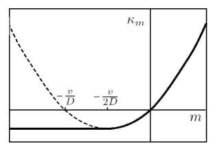
Figure 3: Parameter $\kappa_{m}$ in Eq.30 as a function of $m$. The solid line is realized, if restriction $\rho\mathbin{\lower 3.0pt\hbox{$\hbox to0.0pt{\raise 5.0pt\hbox{$\char 62\relax$}\hss}\mathchar 29208\relax$}}1$ is accepted for the log-normal distribution (10), while the dotted line corresponds to absence of such restriction .

Since $\kappa_{m}$ are negative for negative $m$, it is convenient to set

$$\kappa_{-m}=-\tilde{\kappa}_{m}\,,\qquad m>0\,,$$

so equation for $P(\chi)$ accepts the form

$$\frac{\partial P}{\partial L}=c_{1}{\rm e}^{-\tilde{\kappa}_{1}L}P^{\prime}_{\chi}+c_{2}{\rm e}^{-\tilde{\kappa}_{2}L}P^{\prime\prime}_{\chi\chi}\,,$$

and can be solved iteratively for large $L$,

$$P_{L}(\chi)=P_{\infty}(\chi)-\frac{c_{1}}{\tilde{\kappa}_{1}}{\rm e}^{-\tilde{\kappa}_{1}L}P_{\infty}^{\prime}(\chi)-\frac{c_{2}}{\tilde{\kappa}_{2}}{\rm e}^{-\tilde{\kappa}_{2}L}P_{\infty}^{\prime\prime}(\chi)\,,$$

where $P_{\infty}(\chi)$ is the limiting distribution at $L\to\infty$.

Let mark the points $\tilde{\cal E}_{1}$ and $\tilde{\cal E}_{2}$ in Fig.1,b, corresponding to conditions $v=2D$ and $v=4D$. If the log-normal distribution (10) was valid for arbitrary $\rho$, then the striking phase transition would occur at the point $\tilde{\cal E}_{1}$, relating with sign reversal of $\tilde{\kappa}_{2}$ (the point $-v/D$ in Fig.3 coincide with $-2$ at $\tilde{\cal E}=\tilde{\cal E}_{1}$, so $\tilde{\kappa}_{2}>0$ for $\tilde{\cal E}<\tilde{\cal E}_{1}$ and $\tilde{\kappa}_{2}<0$ for $\tilde{\cal E}>\tilde{\cal E}_{1}$). Then the effective diffusion constant in Eq.33 would grow with $L$ for $\tilde{\cal E}>\tilde{\cal E}_{1}$, and would decrease for $\tilde{\cal E}<\tilde{\cal E}_{1}$. For large $L$, the distribution $P(\chi)$ would be homogeneous with high accuracy for $\tilde{\cal E}>\tilde{\cal E}_{1}$, while the non-trivial distribution $P_{\infty}(\chi)$ would be stabilized for $\tilde{\cal E}<\tilde{\cal E}_{1}$.

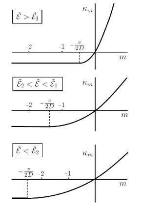
Figure 4: Mutual position of the points $-v/2D$, $-1$ and $-2$ for $\tilde{\cal E}>\tilde{\cal E}_{1}$, $\tilde{\cal E}_{2}<\tilde{\cal E}<\tilde{\cal E}_{1}$ and $\tilde{\cal E}<\tilde{\cal E}_{2}$.

Due to restriction $\rho\mathbin{\lower 3.0pt\hbox{$\hbox to0.0pt{\raise 5.0pt\hbox{$\char 62\relax$}\hss}\mathchar 29208\relax$}}1$ such striking phase transition is not realized , but the point $\tilde{\cal E}_{1}$ remains singular; analogous singularity arises at the point $\tilde{\cal E}_{2}$. As should be clear from Fig.4, the point $-v/2D$, corresponding to matching of the parabola and constant, is situated on the right of the point $-1$ for $\tilde{\cal E}>\tilde{\cal E}_{1}$, and

$$\tilde{\kappa}_{1}=\tilde{\kappa}_{2}\quad\mbox{\rm for}\quad\tilde{\cal E}>\tilde{\cal E}_{1}\,.$$

For the energy interval $\tilde{\cal E}_{2}<\tilde{\cal E}<\tilde{\cal E}_{1}$, the point $-v/2D$ is located between values $-2$ and $-1$, while for the interval $\tilde{\cal E}<\tilde{\cal E}_{2}$ it appears on the left of the point $-2$. One can see, that $\tilde{\kappa}_{1}$ has a jump of the second derivative at $\tilde{\cal E}=\tilde{\cal E}_{1}$, while $\tilde{\kappa}_{2}$ has the analogous jump at $\tilde{\cal E}=\tilde{\cal E}_{2}$. These singularities can be easily registered experimentally, using the treatment based on Eq.34. It is sufficient to find the limiting distribution $P_{\infty}(\chi)$ and fit $P_{L}(\chi)$ by dependence $aP_{\infty}+bP^{\prime}_{\infty}+cP^{\prime\prime}_{\infty}$: it is the linear fitting procedure, which is easily realized by standard routines [30]. Condition (15) corresponds to a large concentration of weak scatterers: in this case, coefficients in Eq.27 changes slowly, which leads to formation of the Gaussian distribution for $P(\chi)$ with variable parameters . It is determined by the first two moments, which significantly simplifies a treatment procedure.

6. Possibilities of measurements in single-mode waveguides

6.1. Analogy with optics

Localization of classical waves was discussed in a number of papers [23]–[29], [10, 11]. It includes consideration of weak [24] and strong [25, 26] localization, absorption near a photon mobility edge [23], near-field mapping of intensity of optical modes in disordered waveguides [27], and many other aspects (see the review article [28]). The transfer matrix approach to the problem was discussed in [10, 11, 29]. In application to optics the corresponding analysis reduces to a set of simple relations.

Propagation of electromagnetic waves in homogeneous dielectric media is described by the wave equation

$$c^{2}\Delta\Psi-n^{2}\frac{\partial^{2}\Psi}{\partial t^{2}}=0\,,$$

where $\Psi$ is any component of the electric or magnetic field. If a medium is spatially inhomogeneous, the refractive index $n$ fluctuates along the coordinate $x$,

$$n^{2}(x)=n_{0}^{2}+\delta n^{2}(x)\,,$$

and for the monochromatic wave $\Psi\sim e^{i\omega t}$, the wave equation can be written in the form

$$\tilde{c}^{2}\Delta\Psi+\left[\omega^{2}+\omega^{2}\frac{\delta n^{2}(x)}{n_{0}^{2}}\right]\Psi=0\,,\qquad\tilde{c}=c/n_{0}\,.$$

The latter exhibits the same structure, as the Schr${\rm\ddot{o}}$dinger equation for an electron with energy ${\cal E}$ and mass $m$ in the random potential $V(x)$. One can easily establish the correspondence

$${\cal E}\,\Longleftrightarrow\,\omega^{2}\,,\quad\frac{1}{2m}\,\Longleftrightarrow\,\tilde{c}^{2}\,,\quad V(x)\,\Longleftrightarrow\,-\omega^{2}\frac{\delta n^{2}(x)}{n_{0}^{2}}\,.$$

A certain difference from the condensed matter physics is related to the $\omega$ dependence of the effective potential $V(x)$, which of little importance, if one is restricted by a small frequency interval of the continuous spectrum.

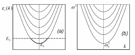
Figure 5: The spectrum of electrons in the metallic wire (a), and the spectrum of waves in a metallic waveguide (b).

The spectrum of waves propagating in a metallic waveguide is analogous to the spectrum of electrons in a metallic wire. In the latter case, the transverse motion is quantized, leading to a set of the discrete levels $\epsilon_{s}$. If the longitudinal motion is taken into account, these levels transform to one-dimensional bands with the dispersion law (Fig.5,a)

$$\epsilon_{s}(k)=\epsilon_{s}+k^{2}/2m\,.$$

To obtain a strictly 1D system, one should have a sufficiently small Fermi level so that only the lowest band is occupied. In the presence of impurities, the lower boundary $\epsilon_{0}$ of the spectrum is smeared out due to the appearance of fluctuation states for ${\cal E}<\epsilon_{0}$. The dependencies shown in Fig.1 correspond to the energy ${\cal E}$ counted from $\epsilon_{0}$.

Analogously, quantization of the transverse motion in a metallic waveguide leads to a set of discrete frequencies $\omega_{s}=\tilde{c}\kappa_{s}$, where $-\kappa_{s}^{2}$ are eigenvalues of the 2D Laplace operator with the appropriate boundary conditions [31]. The zero eigenvalue is possible only in the case, when the waveguide cross-section is multiply connected (e.g. as in a coaxial cable). For a singly connected cross-section, the minimum eigenvalue $\omega_{0}$ is finite [31]. If the longitudinal motion is taken into account, the following branches of the spectrum are obtained (Fig.5,b)

$$\omega^{2}_{s}(k)=\omega_{s}^{2}+\tilde{c}^{2}k^{2}\,.$$

To realize a single-mode regime, one should operate near the lower boundary $\omega_{0}$ of the spectrum. In the presence of disorder, the spectrum boundary $\omega_{0}$ is smeared out due to the occurrence of the fluctuation states. Overall, the effects appearing in the electron system under the change of the Fermi level can be observed in a single-mode waveguide under the change of frequency $\omega$ in the vicinity of $\omega_{0}$.

The spectrum in Fig.5,b corresponds to a metallic waveguide, which is simply a hollow metal tube, which can be also filled by non-absorptive dielectric. The latter case (a metal-coated dielectric waveguide) is of the main interest for our purposes due to possibility of addition of impurities providing sufficiently strong elastic scattering. The coating thickness should be of the order of the skin depth in order to allow for partial field penetration (see Sec.6.4). The transverse motion in the metallic waveguide is restricted by the potential well with infinite walls, so multiplication by $\omega^{2}$ (see (39)) has no effect, and parameters $\kappa_{s}$ are constants, depending only on the form of the waveguide cross-section; correspondingly, the spectrum in Fig.5,b is strictly parabolic.

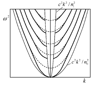
Figure 6: A spectrum of waves in a dielectric waveguide, with the refractive index $n_{0}$ inside the waveguide and $n_{1}$ in environment. For large $\omega$ the spectrum is the same as in metallic waveguide (walls of the potential well are almost infinite); if $\omega$ is diminished, then deviations arise from the parabolic dependencies shown by dotted lines. The lower restrictions for the allowed values of the longitudinal momenta $k$ arise due to violation of conditions for the total internal reflection. Disappearance of the boundary frequency $\omega_{0}$ is related with the fact, that $\kappa_{0}^{2}$ is restricted by the depth of the potential well, proportional to $\omega^{2}$.

In the absence of metal coating (a pure dielectric waveguide), the transverse motion is restricted by the potential well with finite walls, and the frequency dependence of the effective potential $V(x)$ (see Eq.39) becomes essential. Parameters $\kappa_{s}$ cease to be constant and become $\omega$-dependent, resulting in deviations from the parabolic dependencies in Fig.5,b. In particular, the quantity $\kappa_{0}^{2}$ is restricted by the depth of the potential, proportional to $\omega^{2}$, which leads to disappearance of the boundary frequency $\omega_{0}$ (Fig.6). In addition, the lower restrictions for the allowed values of the longitudinal momenta $k$ arise, related with violation of conditions for the total internal reflection. In the usual Schr${\rm\ddot{o}}$dinger equation, the bound states in the potential well $V(x)$ correspond to the energy interval $V_{min}<{\cal E}<V_{\infty}$, where $V_{min}$ is the minimal value of the potential $V(x)$, and $V_{\infty}$ is its limiting (constant) value at infinity. The corresponding condition in the dielectric waveguide has a form $n_{1}^{2}\omega^{2}<c^{2}k^{2}<n_{0}^{2}\omega^{2}$, where $n_{0}$ and $n_{1}$ are refractive indices inside the waveguide and in its environment: correspondingly, the spectrum of waves in the waveguide is restricted by two parabolas (Fig.6).

One can see that a pure dielectric waveguide does not provide a complete analogy with the electron disordered systems: there is nothing that correspond to a forbidden band, and certain differences occur near the band edge. However, the allowed band is achievable for investigation : in particular, the phase transition in $P(\psi)$ is situated in the allowed band and may survive in a dielectric waveguide (though it cannot be stated on a formal level). Its existence looks probable for a sufficiently strong disorder, when the transition is expected in the region where the actual spectrum is close to a parabolic one.

Let a wave of the unit amplitude be incident from the left side of a single-mode waveguide, and comes through it with the amplitude $t$, being reflected with the amplitude $r$. If there are point scatterers in the waveguide, then a partial reflection occurs at any of them. Thus, at an arbitrary point $x$ of the waveguide one finds a superposition of two waves, propagating in opposite directions. The electric field $E(x,t)$ is determined by the real part of this superposition, i.e.

$$E(x,t)={\rm Re}\left[Ae^{ikx+i\omega t}+Be^{-ikx+i\omega t}\vphantom{L^{2}_{2}}\right]\,.$$

With the transfer matrix $T$ being defined by Eqs.(1,2), the amplitudes of the transmitted and reflected waves are determined by the expression

$$\left(\begin{array}[]{cc}A\\ B\end{array}\right)\,=T\,\left(\begin{array}[]{cc}t\\ 0\end{array}\right)=\left(\begin{array}[]{cc}|t|\sqrt{\rho\!+\!1}\,e^{i\varphi-i\varphi_{0}}\\ |t|\sqrt{\rho}\,e^{-i\theta-i\varphi_{0}}\end{array}\right)\,,$$

where $\rho$, $\varphi$, $\theta$ are $x$-dependent and $t=|t|e^{-i\varphi_{0}}$ is accepted. If the amplitude $|t|$ is sufficiently small, then the quantity $\rho$ is large in the whole waveguide, except the vicinity of its right end. Then $|A|\approx|B|$, and Eq.42 gives in this approximation

$$E(x,t)=\!{\rm Re}\!\left[|A|\,e^{ikx+i\omega t+i\varphi-i\varphi_{0}}\!+\!|B|\,e^{-ikx+i\omega t-i\theta-i\varphi_{0}}\vphantom{L^{2}_{2}}\right]$$

$$\approx 2|A|\cos{\left(kx+\chi/2\right)}\cos{\left(\omega t-\psi/2-\varphi_{0}\right)}\,,$$

so the phase $\chi$ controls the coordinate dependence, while $\psi$ controls the time dependence. The phases $\psi$ and $\chi$ remain constant between scatterers, and change abruptly when passing through a scatterer. If the concentration of impurities is large, then $\psi$ and $\chi$ change with $x$ practically continuously, having random variations on the scale of the scattering length.

Since the field $E(x,t)$ can be measured in principle, both phases $\chi$ and $\psi$ are theoretically observable. This is the fundamental difference from the condensed matter physics, where a superposition of waves refers to a wave function, and should be squared in modulus to obtain the observable quantities: in this case the phase $\psi$ is unobservable in principle. This phase would become unobservable in optics, if only the average intensity could be measured (it means that equation (44) is squared and averaged over time). It is easy to verify, that this conclusion remains valid also for $|A|\neq|B|$.

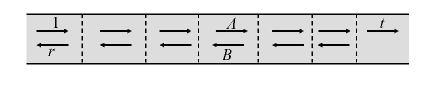
Figure 7: Propagation of waves in the single-mode waveguide with point scatterers.

Nevertheless, the occurrence of the imaginary part of $\psi$ can be registered even in this case. If we suppose that

$$\varphi=\varphi^{\prime}+i\varphi^{\prime\prime}\,,\qquad\theta=\theta^{\prime}+i\theta^{\prime\prime}\,,$$

then the amplitudes in the linear combination (42) accept the form

$$|A|=|t|\sqrt{\rho\!+\!1}\,e^{-\varphi^{\prime\prime}}\,,\qquad|B|=|t|\sqrt{\rho}\,e^{\theta^{\prime\prime}}\,.$$

The flux conservation requires  that the condition $|A|^{2}=|B|^{2}+|t|^{2}$ be fulfilled at the arbitrary point of the waveguide, which leads to relation

$$(\rho\!+\!1)\,e^{-\varphi^{\prime\prime}}=\rho\,e^{\theta^{\prime\prime}}+1$$

giving $\theta^{\prime\prime}=-\varphi^{\prime\prime}$ for large $\rho$. The imaginary part is absent in the phase $\chi$, but is admissible for the phase $\psi$; in the latter case $\psi^{\prime\prime}=2\theta^{\prime\prime}=-2\varphi^{\prime\prime}$, and in particular

$$|A|=|t|\sqrt{\rho\!+\!1}\,e^{\psi^{\prime\prime}/2}\,.$$

The critical behavior of the imaginary part of $\psi$ can be established from the general considerations. Let we have the equation $F(x)=0$, where the function $F(x)$ depends regularly on the external parameter $\epsilon$. If at the point $\epsilon=0$ two real roots become complex-valued, then the multiple root $x=p$ takes place for $\epsilon=0$, and in its vicinity one has the equation (the first derivative over $\epsilon$ is supposed to be finite)

$$(x-p)^{2}-a\epsilon=0\,,$$

which gives roots $p\pm\sqrt{a\epsilon}$ for $a\epsilon>0$ and roots $p\pm i\sqrt{|a\epsilon|}$ for $a\epsilon<0$. Thereby, the appearance of the imaginary part is related with a square root singularity. According to Sec.3, the imaginary part of $\psi$ arises in the result of a choice of parameters $s$ and $w_{0}$, providing the correct values of $v$ and $D$ in the log-normal distribution (10). Thereby, the parameters $s$ and $w_{0}$ are determined by solution of certain equations, whose numerical analysis shows [17], that appearance of the imaginary part of $w_{0}$ is related with confluence of two real roots and their subsequent shift to the complex plane . Hence, the above considerations are immediately applicable to this situation: if the imaginary part of $\psi$ appears for $\omega<\omega_{c}$, then it has a behavior 

$$\psi^{\prime\prime}\sim\sqrt{\omega_{c}-\omega}\,\Theta(\omega_{c}-\omega)\,.$$

According to [17], the distribution $P(\rho)$ is not singular at the point $\omega_{c}$ (Fig.1,b). It refers to a value of $\rho$ at the arbitrary point of the waveguide, and in particular to its value at the whole length $L$, which is related with $t$ as $|t|=(1+\rho)^{-1/2}$. Therefore, the singularity in the amplitude (48) is completely determined by the quantity $\psi^{\prime\prime}$ and has a square root character. The square roots singularities at the point ${\cal E}_{0}$ are visually distinguishable in Figs.8,11 of the paper [17], though obtained by numerical analysis.

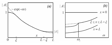
Figure 8: (a) Dependence of the amplitude $|A|$ of the transmitted wave on the coordinate $x$ inside the waveguide. (b) The amplitude $|A|$ versus a frequency $\omega$ in the vicinity of the phase transition.

The general picture looks as follows (Fig.8). In whole, the modulus of $A$ changes in the waveguide according to the exponential law, $|A|\sim e^{-\alpha x}$, but deviations from it arise on the scale $\xi$ near the ends due to influence of boundary conditions (Fig.8,a): in particular, $|A|=1$ for $x=0$ and $|A|=|t|$ for $x=L$. The latter quantity is related with $\rho$ and is a regular function of $\omega$. However, in the deep of the waveguide the amplitude $|A|$ has a square root singularity (Fig.8,b), which can be registered already in the measurements of the average intensity. Such singularity can be observed at the specific point of the system for a specific realization of the potential, since the transition from the true transfer matrix to the pseudo one occurs at the energy corresponding to the renormalized band edge shifted due to a random potential . This shift changes from a point to point (see Footnote 2), but for the distribution $P(\psi)$ in whole corresponds to a strictly defined energy; the latter leads to square root singularities for the moments of this distribution (see the end of Sec.6.3).

According to [17], the critical point ${\cal E}_{0}$ is situated in the allowed band at the distance of order $W^{4/3}$ from the band edge (Fig.1,b). Correspondingly, in optics the critical point $\omega_{c}$ is greater than the boundary frequency $\omega_{0}$, while a distance between them is determined by the degree of disorder.

6.3. Observability of phases $\psi$ and $\chi$

Measurements of the time dependence at optical frequencies are usually impossible. However, observability of the phase $\psi$ can be provided with heterodyne technique, in which the measured electric field $E(x,t)$ is mixed with the additional field $E_{s}(x,t)$, whose frequency is shifted by a small quantity $\Omega$:

$$E+E_{s}={\rm Re}\left\{|E|e^{i\omega t+i\varphi_{E}}+|E_{s}|e^{i(\omega+\Omega)t+i\varphi_{s}}\right\}\,.$$

Considering the intensity averaged over fast time oscillations, one has

$$2\overline{(E+E_{s})^{2}}=|E|^{2}+|E_{s}|^{2}+2|E||E_{s}|\cos{\left(\Omega t+\varphi_{s}-\varphi_{E}\right)}\,,$$

so the phase $\psi$ appears in combination with the slow time dependendence, which can be measured by usual methods. Substituting $E(x,t)$, corresponding to expression (44), one obtains

$$2\overline{(E+E_{s})^{2}}=\left\{4|A|^{2}\cos^{2}{\left(kx+\chi/2\right)}+|E_{s}|^{2}\right\}+$$

$$+2|A|\cos{\left(kx+\chi/2\right)}\cdot 2|E_{s}|\cos{\left(\Omega t+\psi/2+\varphi_{0}+\varphi_{s}\right)}\,,$$

so both phases $\chi$ and $\psi$ are observable, and can be extracted from the experiment by the following treatment.

The stationary first term and the oscillatory second term in Eq.53 can be separated by the Fourier analysis in the time domain. The constant term $|E_{s}|^{2}$ can then be easily extracted, since the smallest value of the first term in the braces is zero. Since the cosine changes regularly and reverses sign at any zero, the square root from the first term in the braces can be extracted to inessential common sign. As a result, two combinations would separately become known

$$|A|\cos{\left(kx+\chi/2\right)}\,\,\,\mbox{\rm and}\,\,\,|E_{s}|\cos{\left(\Omega t+\psi/2+\varphi_{0}+\varphi_{s}\right)}\,.$$

The factor $|E_{s}|$ in the second combination is determined by the amplitude of its temporal oscillations , while its $x$ dependence can be attributed to the spatial dependence of the phase $\psi$.

The treatment of the first combination (54) is complicated by the fact that the amplitude $|A(x)|$ does not follow strictly the exponential dependence $\exp(-\alpha x)$, but exhibits significant fluctuations around it according to the log-normal distribution (10). The appropriate treatment looks as follows:

1. Find a value of $k$ by evaluating the average spatial period of oscillations.

2. Find values of $\chi$ at the sequence of discrete points, which are maxima, minima and zeroes of the oscillating dependence, by assessing deviations of their position from those of the purely cosine function. If the value of $k$ is estimated correctly, then the obtained $\chi$ values would fluctuate around a constant level and not exhibit a systematic growth. As a result, one can gather statistics for the analysis of the $\chi$ distribution.

3. Find values of $|A(x)|$ at the points of maxima and minima. These values would provide the data array for verifying the log-normal distribution and revelation of systematic deviations from the exponential dependence near the waveguide ends.

Observability of the phase $\psi$ provides additional possibilities for registration of the phase transition. If one introduce the variable $w$ defined in Eq.(11), then the moments of the distribution $P(w)$ (e. g. $\langle w\rangle$) will have the singularities $\sqrt{\omega-\omega_{c}}$ in the region $\omega>\omega_{c}$. The phase $\chi$ does not affect the evolution of $P(\rho)$ and was not studied in the papers [16, 17]. However, the possibility of its observation in optics makes such studies to be actual.

6.4. The general measurement scheme

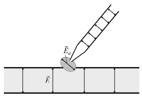
Figure 9: Measurement of the electrical field in a waveguide, using the scanning near-field microscope in the detecting regime.

The electrical field in a waveguide can be measured using methods of the scanning near-field optical microscopy [33, 34, 35]. There are two variants of the near-field microscope, detecting and scattering, which determinate two possible schemes of measurement. Comparison of these schemes leads to a combined variant, where the problem of detection reduces to the atomic force [37, 38] or tunneling [36] microscopy.

Detecting regime. In this case, the probe of the near-field microscope (a fragment of metal-coated optical fibre) is, in fact, a waveguide with the pointed tip and the hole of sub-wavelength size $d$ (Fig.9). The near field, created by the probe, can be imagined as a ’cloud’ of finite volume $V_{d}\sim d^{3}$ (see Fig.4 in Ref.[35]), with the electrical field $\vec{E}_{d}$ approximately parallel to the field inside the probe. Let the tip of the probe is approaching at some angle to a surface of the given waveguide, so that a certain volume $V$ of the ’cloud’ penetrates inside the waveguide (Fig.9). If $\vec{E}$ is the measured field in the waveguide, then a change of the energy due to penetration of the ’cloud’ is determined by expression

$$\left[(\vec{E}+\vec{E}_{d})^{2}-\vec{E}^{2}-\vec{E}_{d}^{2}\right]\,V=2\vec{E}\cdot\vec{E}_{d}\,V\,.$$

For small displacements $x$ of the probe, the change of the volume is proportional to displacement, $\delta V=Sx$, where $S$ is the square of intersection of the ’cloud’ with a surface of the waveguide. Then a force applied to the probe is given by Eq.55 with replacement of $V$ by $S$. It can be transformed to displacement of the probe, or to the change of the voltage retaining the probe in the fixed state. In fact, the field $\vec{E}_{d}$ is space-dependent, and one should write instead of (55)

$$\int 2\vec{E}\cdot\vec{E}_{d}(\vec{r})\,d^{3}r$$

with integration over the waveguide volume, which reduces to (55) after the rough estimation of the integral.

Assuming $E\sim E_{d}$, and introducing the atomic units of the field strength and a force

$$E_{0}=\frac{e}{a^{2}}\sim 10^{9}\,\mbox{\it volt/cm}\,,\qquad F_{0}=\frac{e^{2}}{a^{2}}\sim 10^{-2}\,\mbox{\it dyne}\,,$$

we have the estimate of the force applied to the probe

$$F\sim F_{0}\left(\frac{E}{E_{0}}\right)^{2}\left(\frac{d}{a}\right)^{2}\,.$$

Since the size of the hole $d$ is restricted by the condition $d\mathbin{\lower 3.0pt\hbox{$\hbox to0.0pt{\raise 5.0pt\hbox{$\char 60\relax$}\hss}\mathchar 29208\relax$}}\lambda\sim 10^{4}a$, we can set

$$F\sim 10^{6}\left(\frac{E}{E_{0}}\right)^{2}\,\mbox{\it dyne}\,.$$

The maximal value of the field is restricted by the field of the dielectric breakdown $\sim 10^{7}volt/cm$. Accepting sensitivity of measurement on the level $F\sim 10^{-8}\mbox{\it dyne}$, typical for the tunneling microscopy [36], we have the wide interval of fields

$$10^{-7}E_{0}\mathbin{\lower 3.0pt\hbox{$\hbox to0.0pt{\raise 5.0pt\hbox{$\char 60\relax$}\hss}\mathchar 29208\relax$}}E\mathbin{\lower 3.0pt\hbox{$\hbox to0.0pt{\raise 5.0pt\hbox{$\char 60\relax$}\hss}\mathchar 29208\relax$}}10^{-2}E_{0}\,,$$

where the described scheme is realistic.

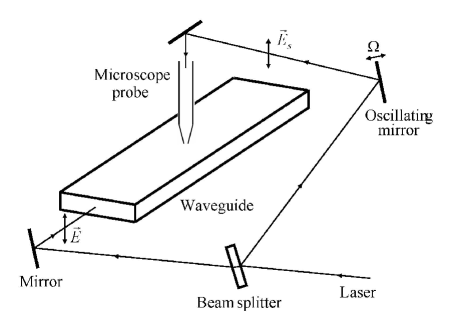
Figure 10: General scheme of measurement in the detecting regime of the scanning near-field optical microscope.

If in the capacity of $\vec{E}_{d}$ we use the field $\vec{E}_{s}$ with a shifted frequency (see Eq.51), then the force applied to the probe is determined by the quantity

$$F\sim S|A||E_{s}|\cos{\left(kx+\chi/2\right)}\cos{\left(\Omega t+\psi/2+\varphi_{0}+\varphi_{s}\right)}\,,$$

whose treatment is even simpler then that of the expression (53). In previous arguments, we did not take into account existence of the semi-transparent metal coating (Sec.6.1) and a difference from unity of the dielectric permeability inside the waveguide. These factors leads to additive contribution of order $E_{s}^{2}$ in the right-hand side of Eq.61, which is independent of the measured field and easily separated in the course of treatment.

The general measurement scheme looks as follows (Fig.10). A laser beam is split into two parts, one of which is directed into the waveguide. The second part of the beam is incident to an oscillating mirror, acquiring a small frequency shift $\Omega$ due to the Doppler effect. Since the mirror velocity is variable, it leads to a variable shift $\Omega$. This problem can be solved by registration of the time dependence at the discrete points, equally spaced by the period of mirror oscillations. Another possibility consists in realization of the saw-toothed regime of oscillations instead of the harmonic one. Leaving the mirror, the beam is directed to the microscope probe. Near a tip of the latter the field $\vec{E}+\vec{E}_{s}$ is created, and measurement of the force (61) allows to determine the coordinate dependence of $\vec{E}$ in the course of scanning of the waveguide surface.

Scattering regime. In this case, an optical microscope probe is used not for the immediate field detection, but only as a source of scattering with subsequent use of a remote detector. A wave propagating in the waveguide penetrates beyond its boundaries due to the tunneling effect and can be scattered by a probe tip located close to a waveguide surface. For sub-wavelength-sized probe tips, the scattering occurs in the Rayleigh regime, with the field of the scattered wave being proportional to the local electric field $E(x,t)$ in the waveguide  at the point of scattering $x$.

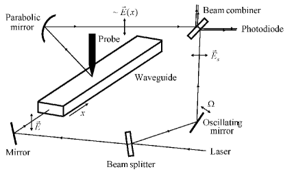
Figure 11: General scheme of measurement in the scattering regime of the scanning near-field optical microscope.

The general scheme of field measurement looks as follows (Fig.11). A laser beam is split into two parts, one of which is directed into a waveguide and eventually scattered by a microscope probe tip. The scattered light is collected by a parabolic mirror and directed to a beam combiner. The second part of the laser beam is reflected by an oscillating mirror, acquiring a small frequency shift $\Omega$ due to the Doppler effect. After the mirror, the beam is directed to the beam combiner, where it is mixed with the first beam and follows to a photodiode for measurement of intensity. The described scheme was realized in studies of the paper [39], where additional experimental details can be found.

Combined scheme differs from Fig.10 only by the fact that the second beam, leaving the oscillating mirror, is directed to the waveguide and comes through it in the transverse direction near its surface (Fig.12). Since the field $\vec{E}$ penetrates beyond the waveguide due to the tunneling effect, the composed field $\vec{E}+\vec{E}_{s}$ is present above its surface. The energy of this field is changed, when the probe tip is approached, due to the dielectric polarization of the latter. As a result, the force applied to the probe is proportional to the intensity of the field $\vec{E}+\vec{E}_{s}$, and the problem of its measurement is reduced to the atomic force [37, 38] or tunneling [36] microscopy.

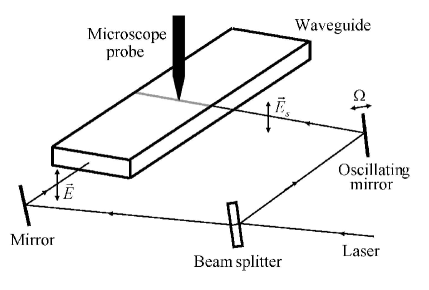
Figure 12: Measurement of the electric field in the waveguide using the atomic force or tunneling microscopy.

7. Conclusion

It has been shown that all results obtained for electrons in 1D disordered systems are immediately applicable to the propagation of electromagnetic waves in single-mode optical waveguides. The modern optical methods enable measurements of all parameters $\rho$, $\psi$, $\chi$, entering the transfer matrix. In particular, it becomes possible to observe the phase transition for the distribution $P(\psi)$, which looks unobservable in the framework of the condensed matter physics. Since the phase $\chi$ becomes observable, one finds it actual to derive the evolution equation for its distribution, which was not studied in previous papers. At large $L$, the distribution of $\chi$ has singularities, consisting in jumps of the second derivative for exponentials, describing relaxation of $P_{L}(\chi)$ to the limiting distribution $P_{\infty}(\chi)$.

As was indicated above, one of the measurement schemes described in Sec.6.4 was realized in the paper [39]. In contrast to studies [40, 41], where only the transmission matrix was measured, Ref.[39] presents the experimental approach allowing to measure the phase distribution inside the waveguide. However, the measurements of Ref.[39] were not concerned with light propagation in disordered systems, but only with characterization of regular modes in homogeneous waveguides.

Essentially new measurements are necessary for testing the validity of claims made in the present paper. The actual experiments should be executed using a tunable laser allowing to change the light frequency, and its tunability range should cover the targeted phase transition. The latter demand to establish the most promising waveguide configuration and dimensions. A suitable approach should be developed for introducing a large concentration of impurities into the waveguide. Extensive analysis is necessary to find the parameter range, where the localization effects will be dominating over the light absorption inside the waveguide and radiative losses through its boundaries. The latter problem is somewhat facilated for a pure dielectric waveguide, but then the analogy with electronic systems becomes incomplete (Sec.6.1).

One can hope that the obtained results might stimulate the corresponding experimental activities that would, in turn, shed more light on intricate effects in both optical and electron localization phenomena.

The author is indebted to S.I.Bozhevolnyi for numerous discussions of the optical aspects of this paper.

Appendix.   Evolution equation for $P(\rho,\psi,\chi)$

The method for derivation of the evolution equation presented below is somewhat different from that in the papers [16, 17]: it is more systematic and ensures attainment of a result when its character is unknown beforehand. The more compact way of derivation [16, 17] can be found only in the presence of a certain information on the structure of the result.

As clear from relations (18), (19), (20), (22), the phase $\psi$ enters evolution equations in the form of two combinations $\psi-\gamma$ and $\psi-\beta$, so the shift $\psi\to\psi+\psi_{0}$ allows to reduce the parameter $\gamma$ to the value $-\pi/2$, corresponding to abrupt interfaces between the system and the ideal leads [17]; to simplify formulas, we restrict ourselves by this case. Relations (12–14) give in the main order in $\delta$

$$T^{(n+1)}_{11}=(1+i\alpha-i\epsilon_{n})T^{(n)}_{11}+(\delta_{1}-i\delta_{2}+i\epsilon_{n})T^{(n)}_{12}$$

$$T^{(n+1)}_{12}=(\delta_{1}+i\delta_{2}-i\epsilon_{n})T^{(n)}_{11}+(1-i\alpha+i\epsilon_{n})T^{(n)}_{12}$$

and analogous equations for $T^{(n)}_{21}$ and $T^{(n)}_{22}$, obtained by complex conjugation; here $\delta_{1}=\Delta\cos\beta$, $\delta_{2}=\Delta\sin\beta$. Setting

$$T^{(n)}_{11}=x_{n}+iy_{n}\,,\qquad T^{(n)}_{12}=z_{n}+iw_{n}\,,$$

we have

$$x_{n+1}=x_{n}-(\alpha-\epsilon_{n})y_{n}+\delta_{1}z_{n}-(\delta_{2}+\epsilon_{n})w_{n}$$

$$y_{n+1}=(\alpha-\epsilon_{n})x_{n}+y_{n}+(\delta_{2}+\epsilon_{n})z_{n}+\delta_{1}w_{n}$$

$$z_{n+1}=\delta_{1}x_{n}+(\delta_{2}+\epsilon_{n})y_{n}+z_{n}+(\alpha-\epsilon_{n})w_{n}$$

$$w_{n+1}=-(\delta_{2}+\epsilon_{n})x_{n}+\delta_{1}y_{n}-(\alpha-\epsilon_{n})z_{n}+w_{n}$$

which after rewriting in the matrix form gives the matrix with the unit determinant. If the distribution $P_{n}(x_{n},y_{n},z_{n},w_{n})$ is known, then the analogous distribution at the $(n+1)$th step is composed according to the rule

$$P_{n+1}(\tilde{x}_{n+1},\tilde{y}_{n+1},\tilde{z}_{n+1},\tilde{w}_{n+1})=\int d\epsilon_{n}dx_{n}\,dy_{n}\,dz_{n}\,dw_{n}\cdot$$

$$\cdot P(\epsilon_{n})\,P_{n}(x_{n},y_{n},z_{n},w_{n})\delta\left(\tilde{x}_{n+1}-x_{n+1}\right)\cdot$$

$$\cdot\delta\left(\tilde{y}_{n+1}-y_{n+1}\right)\delta\left(\tilde{z}_{n+1}-z_{n+1}\right)\delta\left(\tilde{w}_{n+1}-w_{n+1}\right)\,,$$

where $x_{n+1}$, $y_{n+1}$, $z_{n+1}$, $w_{n+1}$ are expressed in terms of $x_{n}$, $y_{n}$, $z_{n}$, $w_{n}$ according to $(A.3)$. Let inverse the relation $(A.3)$ and come to integration over $x_{n+1}$, $y_{n+1}$, $z_{n+1}$, $w_{n+1}$; since the Jacobian is equal to unity and $\delta$-functions are trivially removed, we come to equation

$$P_{n+1}(x_{n+1},y_{n+1},z_{n+1},w_{n+1})=\qquad\qquad\qquad$$

$$\qquad\qquad\qquad=\int d\epsilon_{n}P(\epsilon_{n})P_{n}(x_{n},y_{n},z_{n},w_{n})\,,$$

where $x_{n}$, $y_{n}$, $z_{n}$, $w_{n}$ are expressed through $x_{n+1}$, $y_{n+1}$, $z_{n+1}$, $w_{n+1}$ by the relation inverse to $(A.3)$. Expanding over differences $x_{n+1}-x_{n}$, $y_{n+1}-y_{n}$, $\dots$ and retaining the terms of the first order in $\delta$ and second order in $\epsilon$, we have

$$\frac{\partial P}{\partial n}=\alpha\left[y\frac{\partial P}{\partial x}-x\frac{\partial P}{\partial y}-w\frac{\partial P}{\partial z}+z\frac{\partial P}{\partial w}\right]-$$

$$-\delta_{1}\left[z\frac{\partial P}{\partial x}+w\frac{\partial P}{\partial y}+x\frac{\partial P}{\partial z}+y\frac{\partial P}{\partial w}\right]+$$

$$+\delta_{2}\left[w\frac{\partial P}{\partial x}-z\frac{\partial P}{\partial y}-y\frac{\partial P}{\partial z}+x\frac{\partial P}{\partial w}\right]+$$

$$+\frac{1}{2}\epsilon^{2}(w\!-\!y)^{2}\left[\frac{\partial^{2}P}{\partial x^{2}}+2\frac{\partial^{2}P}{\partial x\partial z}+\frac{\partial^{2}P}{\partial z^{2}}\right]+$$

$$+\frac{1}{2}\epsilon^{2}(x\!-\!z)^{2}\left[\frac{\partial^{2}P}{\partial y^{2}}+2\frac{\partial^{2}P}{\partial y\partial w}+\frac{\partial^{2}P}{\partial w^{2}}\right]+$$

$$+\epsilon^{2}(x\!-\!z)(w\!-\!y)\left[\frac{\partial^{2}P}{\partial x\partial y}+\frac{\partial^{2}P}{\partial x\partial w}+\frac{\partial^{2}P}{\partial z\partial y}+\frac{\partial^{2}P}{\partial z\partial w}\right]\,.$$

Introducing the polar coordinates

$$x=r_{1}\cos\varphi,\quad y=r_{1}\sin\varphi,\quad z=r_{2}\cos\theta,\quad w=r_{2}\sin\theta\,,$$

we obtain

$$\frac{\partial P}{\partial n}=\alpha\left[-P^{\prime}_{\varphi}+P^{\prime}_{\theta}\right]-\Delta\cos(\theta-\varphi-\beta)\left[r_{2}P^{\prime}_{r_{1}}+r_{1}P^{\prime}_{r_{2}}\right]+$$

$$+\Delta\sin(\theta\!-\!\varphi\!-\!\beta)\left[\frac{r_{1}}{r_{2}}P^{\prime}_{\theta}-\frac{r_{2}}{r_{1}}P^{\prime}_{\varphi}\right]+$$

$$+\frac{1}{2}\epsilon^{2}\left\{\vphantom{\left[\frac{1}{r^{2}_{2}}P^{\prime\prime}_{\theta\theta}\right]}\sin^{2}(\theta\!-\!\varphi)\left[r^{2}_{2}P^{\prime\prime}_{r_{1}r_{1}}+2r_{1}r_{2}P^{\prime\prime}_{r_{1}r_{2}}+r^{2}_{1}P^{\prime\prime}_{r_{2}r_{2}}\right]\right.+$$

$$\left.+2\sin(\theta\!-\!\varphi)\left[\vphantom{r^{2}_{2}P^{\prime\prime}_{r_{1}r_{1}}}r_{1}-r_{2}\cos(\theta\!-\!\varphi)\right]\left[\frac{r_{2}}{r_{1}}P^{\prime\prime}_{r_{1}\varphi}+P^{\prime\prime}_{r_{2}\varphi}-\frac{r_{2}}{r^{2}_{1}}P^{\prime}_{\varphi}\right]\right.$$

$$\left.+2\sin(\theta\!-\!\varphi)\left[\vphantom{r^{2}_{2}P^{\prime\prime}_{r_{1}r_{1}}}r_{1}\cos(\theta\!-\!\varphi)-r_{2}\right]\left[\frac{r_{1}}{r_{2}}P^{\prime\prime}_{r_{2}\theta}+P^{\prime\prime}_{r_{1}\theta}-\frac{r_{1}}{r^{2}_{2}}P^{\prime}_{\theta}\right]\right.$$

$$+\left[\vphantom{r^{2}_{2}P^{\prime\prime}_{r_{1}r_{1}}}r_{1}-r_{2}\cos(\theta\!-\!\varphi)\right]^{2}\left[\frac{1}{r^{2}_{1}}P^{\prime\prime}_{\varphi\varphi}+\frac{1}{r_{1}}P^{\prime}_{r_{1}}\right]+$$

$$+\left[\vphantom{r^{2}_{2}P^{\prime\prime}_{r_{1}r_{1}}}r_{1}\cos(\theta\!-\!\varphi)-r_{2}\right]^{2}\left[\frac{1}{r^{2}_{2}}P^{\prime\prime}_{\theta\theta}+\frac{1}{r_{2}}P^{\prime}_{r_{2}}\right]+$$

$$\left.+2\left[\vphantom{r^{2}_{2}P^{\prime\prime}_{r_{1}r_{1}}}r_{1}-r_{2}\cos(\theta\!-\!\varphi)\right]\left[\vphantom{r^{2}_{2}P^{\prime\prime}_{r_{1}r_{1}}}r_{1}\cos(\theta\!-\!\varphi)-r_{2}\right]\frac{1}{r_{1}r_{2}}P^{\prime\prime}_{\varphi\theta}\vphantom{\left[\frac{1}{r^{2}_{2}}P^{\prime\prime}_{\theta\theta}\right]}\right\}\,.$$

Now come from the quantities $r_{1}$, $r_{2}$ to the new variables $\rho$, $\xi$

$$r^{2}_{1}+r^{2}_{2}=1+2\rho\,,\qquad r^{2}_{1}-r^{2}_{2}=\xi\,.$$

On can easily verify, that all terms with derivatives over $\xi$ disappear; hence the quantity $\xi$ remains constant in the course of evolution, and on the physical grounds we can set $\xi=1$. Then

$$r_{1}=\sqrt{1+\rho}\,,\qquad r_{2}=\sqrt{\rho}$$

in correspondence with the canonical representation (2). The corresponding evolution equation accepts the form

$$\frac{\partial P}{\partial n}=\alpha\left[-P^{\prime}_{\varphi}+P^{\prime}_{\theta}\right]-\Delta\cos(\theta\!-\!\varphi\!-\!\beta)2r_{1}r_{2}P^{\prime}_{\rho}+$$

$$+\Delta\sin(\theta\!-\!\varphi\!-\!\beta)\left[\frac{r_{1}}{r_{2}}P^{\prime}_{\theta}-\frac{r_{2}}{r_{1}}P^{\prime}_{\varphi}\right]+$$

$$+\frac{1}{2}\epsilon^{2}\left\{\vphantom{\left[\frac{1}{r^{2}_{2}}P^{\prime\prime}_{\theta\theta}\right]}4r^{2}_{1}r^{2}_{2}\sin^{2}(\theta\!-\!\varphi)P^{\prime\prime}_{\rho\rho}+\right.$$

$$+\left[2r^{2}_{1}+2r^{2}_{2}-4r_{1}r_{2}\cos(\theta\!-\!\varphi)\right]P^{\prime}_{\rho}+$$

$$+4r_{2}\sin(\theta\!-\!\varphi)\left[\vphantom{r^{2}_{2}P^{\prime\prime}_{r_{1}r_{1}}}r_{1}-r_{2}\cos(\theta\!-\!\varphi)\right]P^{\prime\prime}_{\rho\varphi}+$$

$$+4r_{1}\sin(\theta\!-\!\varphi)\left[\vphantom{r^{2}_{2}P^{\prime\prime}_{r_{1}r_{1}}}r_{1}\cos(\theta\!-\!\varphi)-r_{2}\right]P^{\prime\prime}_{\rho\theta}-$$

$$-2\sin(\theta\!-\!\varphi)\frac{r_{2}\left[r_{1}-r_{2}\cos(\theta\!-\!\varphi)\right]}{r_{1}^{2}}P^{\prime}_{\varphi}-$$

$$-2\sin(\theta\!-\!\varphi)\frac{r_{1}\left[r_{1}\cos(\theta\!-\!\varphi)-r_{2}\right]}{r_{2}^{2}}P^{\prime}_{\theta}+$$

$$\left.+\!\left[\frac{r_{1}\!-\!r_{2}\cos(\theta\!-\!\varphi)}{r_{1}}\right]^{2}\!\!P^{\prime\prime}_{\varphi\varphi}+\!\left[\frac{r_{1}\cos(\theta\!-\!\varphi)\!-\!r_{2}}{r_{2}}\right]^{2}\!\!P^{\prime\prime}_{\theta\theta}+\right.$$

$$\left.+2\left[\frac{r_{1}-r_{2}\cos(\theta\!-\!\varphi)}{r_{1}}\right]\left[\frac{r_{1}\cos(\theta\!-\!\varphi)-r_{2}}{r_{2}}\right]\,P^{\prime\prime}_{\varphi\theta}\vphantom{\left[\frac{1}{r^{2}_{2}}P^{\prime\prime}_{\theta\theta}\right]}\right\}\,.$$

In the course of the changes of variables $(A.7)$ and $(A.9)$ we do not produce renormalization of probability; however, in the result of two changes we have

$$4P(x,y,z,w)\,dx\,dy\,dz\,dw=P(\rho,\xi,\varphi,\theta)\,d\rho\,d\xi\,d\varphi\,d\theta\,,$$

and the indicated renormalization reduces to an inessential constant factor. Introducing combined phases (3), one has

$$\frac{\partial P}{\partial n}=2\alpha P^{\prime}_{\psi}-\Delta\cos(\psi\!-\!\beta)2r_{1}r_{2}P^{\prime}_{\rho}+$$

$$+\Delta\sin(\psi\!-\!\beta)\left[\left(\frac{r_{1}}{r_{2}}+\frac{r_{2}}{r_{1}}\right)P^{\prime}_{\psi}+\left(\frac{r_{1}}{r_{2}}-\frac{r_{2}}{r_{1}}\right)P^{\prime}_{\chi}\right]+$$

$$+\frac{1}{2}\epsilon^{2}\left\{\vphantom{\left[\frac{1}{r^{2}_{2}}P^{\prime\prime}_{\theta\theta}\right]}4r^{2}_{1}r^{2}_{2}\sin^{2}{\psi}P^{\prime\prime}_{\rho\rho}+\left[2r^{2}_{1}+2r^{2}_{2}-4r_{1}r_{2}\cos{\psi}\right]P^{\prime}_{\rho}\right.+$$

$$+4\sin{\psi}\left(\vphantom{r^{2}_{2}P^{\prime\prime}_{r_{1}r_{1}}}r_{1}r_{2}-r_{2}^{2}\cos{\psi}\right)\left(-P^{\prime\prime}_{\rho\psi}+P^{\prime\prime}_{\rho\chi}\right)$$

$$+4\sin{\psi}\left(\vphantom{r^{2}_{2}P^{\prime\prime}_{r_{1}r_{1}}}r_{1}^{2}\cos{\psi}-r_{1}r_{2}\right)\left(P^{\prime\prime}_{\rho\psi}+P^{\prime\prime}_{\rho\chi}\right)$$

$$-2\sin{\psi}\left(\frac{r_{2}}{r_{1}}-\frac{r^{2}_{2}}{r^{2}_{1}}\cos{\psi}\right)\left(-P^{\prime}_{\psi}+P^{\prime}_{\chi}\right)$$

$$-2\sin{\psi}\left(\frac{r^{2}_{1}}{r^{2}_{2}}\cos{\psi}-\frac{r_{1}}{r_{2}}\right)\left(P^{\prime}_{\psi}+P^{\prime}_{\chi}\right)$$

$$+\left(\frac{r_{1}-r_{2}\cos{\psi}}{r_{1}}\right)^{2}\left(P^{\prime\prime}_{\psi\psi}-2P^{\prime\prime}_{\psi\chi}+P^{\prime\prime}_{\chi\chi}\right)$$

$$+\left(\frac{r_{1}\cos{\psi}-r_{2}}{r_{2}}\right)^{2}\left(P^{\prime\prime}_{\psi\psi}+2P^{\prime\prime}_{\psi\chi}+P^{\prime\prime}_{\chi\chi}\right)$$

$$\left.+\left(\frac{r_{1}-r_{2}\cos{\psi}}{r_{1}}\right)\left(\frac{r_{1}\cos{\psi}-r_{2}}{r_{2}}\right)\left(-P^{\prime\prime}_{\psi\psi}+P^{\prime\prime}_{\chi\chi}\right)\right\}$$

Substituting $(A.10)$ and transforming the right-hand side to the sum of full derivatives, we come to the final evolution equation, which has a structure of Eq.4:

$$\frac{\partial P}{\partial n}=\left\{\vphantom{\frac{1}{2}}\!\!-2\Delta\!\cos{(\psi\!-\!\beta)}\sqrt{\!\rho(\!1\!+\!\rho\!)}P+2\epsilon^{2}\!\sin\!^{2}{\psi}\,\rho(\!1\!+\!\rho\!)P^{\prime}_{\rho}+\right.$$

$$+\epsilon^{2}\left[(1\!-\!2\sin^{2}{\psi})(1\!+\!2\rho)-2\cos{\psi}\sqrt{\rho(1\!+\!\rho)}\right]P+$$

$$\left.+2\epsilon^{2}\sin{\psi}\left[\cos{\psi}(1\!+\!2\rho)-2\sqrt{\rho(1\!+\!\rho)}\right]P^{\prime}_{\psi}\right\}^{\prime}_{\rho}+$$

$$+\left\{\left[\vphantom{R^{2}}2\alpha\!+\!R\Delta\sin{(\psi\!-\!\beta)}\right]P\vphantom{\frac{1}{2}}+\epsilon^{2}\sin{\psi}(R\!-\!2\cos{\psi})P\right.+$$

$$\left.+\frac{1}{2}\epsilon^{2}(2\!-\!R\cos{\psi})^{2}\,P^{\prime}_{\psi}\right\}^{\prime}_{\psi}\,+$$

$$+\left\{\,\frac{\Delta\sin{(\psi\!-\!\beta)}\!+\!\epsilon^{2}\sin{\psi}\,(1\!-\!R\cos{\psi})}{\sqrt{\rho(1\!+\!\rho)}}\,P\right.$$

$$\left.+\,\frac{\epsilon^{2}\cos{\psi}\,(R\cos{\psi}\!-\!2)}{\sqrt{\rho(1\!+\!\rho)}}\,P^{\prime}_{\psi}+\frac{\epsilon^{2}\cos^{2}{\psi}}{2\rho(1\!+\!\rho)}\,P^{\prime}_{\chi}\,\right\}^{\prime}_{\chi}\,.$$

Integration over $\chi$ gives the evolution equation for $P(\rho,\psi)$, obtained in [16, 17], while integration over $\rho$ and $\psi$ leads to equation (27) for $P(\chi)$.

References

- [1] P. W. Anderson, D. J. Thouless, E. Abrahams, D. S. Fisher, Phys. Rev. B 22, 3519 (1980).
- [2] R. Landauer, IBM J. Res. Dev. 1, 2 (1957); Phil. Mag. 21, 863 (1970).
- [3] V. I. Melnikov, Sov. Phys. Sol. St. 23, 444 (1981).
- [4] A. A. Abrikosov, Sol. St. Comm. 37, 997 (1981).
- [5] N. Kumar, Phys. Rev. B 31, 5513 (1985).
- [6] B. Shapiro, Phys. Rev. B 34, 4394 (1986).
- [7] P. Mello, Phys. Rev. B 35, 1082 (1987).
- [8] B. Shapiro, Phil. Mag. 56, 1031 (1987).
- [9] I. M. Lifshitz, S. A. Gredeskul, L. A. Pastur, Introduction to the Theory of Disordered Systems, Nauka, Moscow, 1982.
- [10] C. W. J. Beenakker, Rev. Mod. Phys. 69, 731 (1997).
- [11] X. Chang, X. Ma, M. Yepez, A. Z. Genack, P. A. Mello, Phys. Rev. B 96, 180203 (2017).
- [12] L. I. Deych, D. Zaslavsky, A. A. Lisyansky, Phys. Rev. Lett. 81, 5390 (1998).
- [13] L. I. Deych, A. A. Lisyansky, B. L Altshuler, Phys. Rev. Lett. 84, 2678 (2000); Phys. Rev. B 64, 224202 (2001).
- [14] L. I. Deych, M. V. Erementchouk, A. A. Lisyansky, Phys. Rev. Lett. 90, 126601 (2001).
- [15] I. M. Suslov, J. Exp. Theor. Phys. 129, 877 (2019) [Zh. Eksp. Teor. Fiz. 156, 950 (2019)].
- [16] I. M. Suslov, Phil. Mag. Lett. 102, 255 (2022).
- [17] I. M. Suslov, J. Exp. Theor. Phys. 135, 726 (2022) [Zh. Eksp. Teor. Fiz. 162, 750 (2022)].
- [18] S. I. Bozhevolnyi, I. M. Suslov, Phys. Scr. 98, 065024 (2023).
- [19] I. M. Suslov, Adv. Theor. Comp. Phys. 6, 77 (2023).
- [20] N. F. Mott, E. A Davis, Electron Processes in Non-Crystalline Materials, Oxford, Clarendon Press, 1979.
- [21] V. V. Brazhkin, I. M. Suslov, J. Phys. – Cond. Matt. 32 (35), 35LT02 (2020).
- [22] I. M. Suslov, J. Exp. Theor. Phys. 131, 793 (2020) [Zh. Eksp. Teor. Fiz. 158, 911 (2020)].
- [23] S. John, Phys. Rev. Lett. 53, 2169 (1984).
- [24] P. Van Albada, A. Lagendijk, Phys. Rev. Lett. 55, 2692 (1985).
- [25] P. W. Anderson, Phil. Mag. B 52, 505 (1985).
- [26] S. John, Phys. Rev. Lett. 58, 2486 (1987).
- [27] S. I. Bozhevolnyi, V. S. Volkov, K. Leosson, Phys. Rev. Lett. 89, 186801 (2002).
- [28] D. S. Wiersma, Nature Photon. 7, 188 (2013).
- [29] Zh. Shi, M. Davy, A. Z. Genack, Opt. Express 23, 12293 (2015).
- [30] W. H. Press, B. P. Flannery, S. A. Teukolsky, W. T. Wetterling, Numerical Recipes in Fortran, Cambridge University Press, 1992.
- [31] L. D. Landau, E. M. Lifshits, Electrodynamics of Continuous Media, Oxford, Pergamon Press, 1984.
- [32] Ch. K. Kao, Nobel Prize Lecture, 2009.
- [33] D. W. Pohl, W. Denk, M. Lanz, Appl. Phys. Lett. 44, 651 (1984).
- [34] D. W. Pohl, L. Novotny, J. Vac. Sci. Technol. B 12, 1441 (1994).
- [35] A. L. Lereu, A. Passian, Ph. Dumas, Int. J. Nanotechnol. 9, 488 (2012).
- [36] G.Binning, H.Rohrer, Helv. Phys. Acta. 55, 726 (1982).
- [37] G.Binning, C. F. Quate, C. Gerber, Phys. Rev. Lett. 56, 930 (1986).
- [38] E. Meyer, Progress in Surface Science 41, 3 (1992).
- [39] S. I. Bozhevolnyi, V. A. Zenin, R. Malreanu, I. P. Radko, A. V. Lavrinenko, Opt. Express 24, 4582 (2016).
- [40] I. M. Vellekoop and A. P. Mosk, Phys. Rev. Lett. 101, 120601 (2008).
- [41] S. M. Popoff, G. Lerosey, R. Carminati, M. Fink, A. C. Boccara, and S. Gigan, Phys. Rev. Lett. 104, 100601 (2010).